Embed Size (px)
Citation preview

CADSWES
DEPARTMENT
OF
UNIVERSITY OF COLORADO
CENTER FOR ADVANCED
DECISION SUPPORT
FOR
WATER AND ENVIRONMENTAL
SYSTEMS
CIVIL ENGINEERING
A Final Report
Robert L. Runkel
One-Dimensional Transport with Inflow
and Storage (OTIS): A Solute Transport
Model for Small Streams
Robert E. Broshears
September 30, 1991
in cooperation with the
United States Geological Survey
Water Resources Division

One-Dimensional Transport with Inflow and Storage (OTIS)
Acknowledgments
This work was carried out as part of a co-operative agreement between CU-CADSWES and the United States Geological Survey (USGS) in Denver, Colo-rado. Funding for the work was provided by the USGS Toxic SubstancesHydrology Program. The authors wish to thank Kenneth Bencala (USGS-Menlo Park), Briant Kimball (USGS-Salt Lake City), Diane McKnight (USGS-Denver) and Steven Chapra (CU-CADSWES) for their review of this documentand their input during software development. A big ‘thank you’ also goes out toSandra Braitberg and Judith Bond for their help in formatting this documentand the ‘Equations from Hades’.
CADSWES 3
TNEMTR
AP
ED
SU
O F TH E
I NT
ER
IOR
hcraM, 1 8 4 9
Authors:
Robert L. RunkelCU-CADSWES2945 Center Green CourtSuite BBoulder, Colorado 80301
Robert E. BroshearsU.S. Geological SurveyWater Resources DivisionMail Stop 415Denver Federal CenterLakewood, Colorado 80225
One-Dimensional Transport with Inflow and Storage (OTIS)
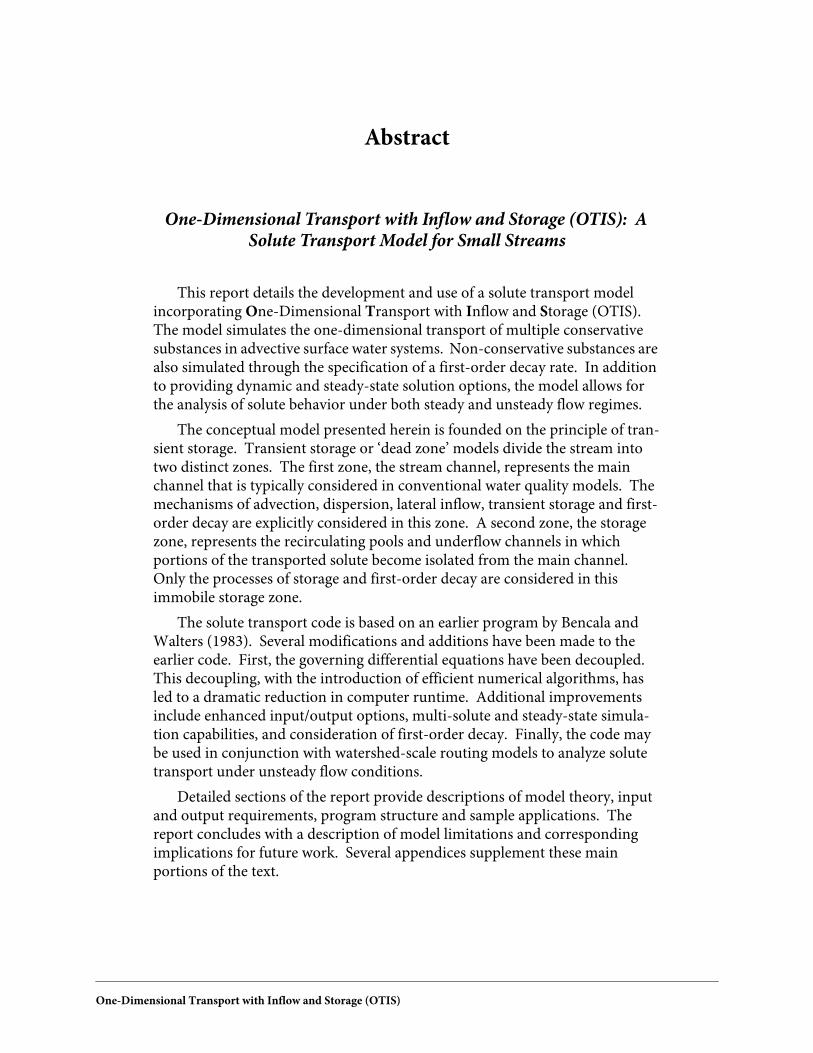
Abstract
One-Dimensional Transport with Inflow and Storage (OTIS): ASolute Transport Model for Small Streams
This report details the development and use of a solute transport modelincorporating One-Dimensional Transport with Inflow and Storage (OTIS).The model simulates the one-dimensional transport of multiple conservativesubstances in advective surface water systems. Non-conservative substances arealso simulated through the specification of a first-order decay rate. In additionto providing dynamic and steady-state solution options, the model allows forthe analysis of solute behavior under both steady and unsteady flow regimes.
The conceptual model presented herein is founded on the principle of tran-sient storage. Transient storage or ‘dead zone’ models divide the stream intotwo distinct zones. The first zone, the stream channel, represents the mainchannel that is typically considered in conventional water quality models. Themechanisms of advection, dispersion, lateral inflow, transient storage and first-order decay are explicitly considered in this zone. A second zone, the storagezone, represents the recirculating pools and underflow channels in whichportions of the transported solute become isolated from the main channel.Only the processes of storage and first-order decay are considered in thisimmobile storage zone.
The solute transport code is based on an earlier program by Bencala andWalters (1983). Several modifications and additions have been made to theearlier code. First, the governing differential equations have been decoupled.This decoupling, with the introduction of efficient numerical algorithms, hasled to a dramatic reduction in computer runtime. Additional improvementsinclude enhanced input/output options, multi-solute and steady-state simula-tion capabilities, and consideration of first-order decay. Finally, the code maybe used in conjunction with watershed-scale routing models to analyze solutetransport under unsteady flow conditions.
Detailed sections of the report provide descriptions of model theory, inputand output requirements, program structure and sample applications. Thereport concludes with a description of model limitations and correspondingimplications for future work. Several appendices supplement these mainportions of the text.

One-Dimensional Transport with Inflow and Storage (OTIS)
One-Dimensional Transport with Inflow and Storage (OTIS):A Solute Transport Model for Small Streams
Table of Contents Page
1.0 INTRODUCTION . . . . . . . . . . . . . . . . . . . . . . . . . . . . . . . . . . . 1
2.0 CONTRIBUTIONS . . . . . . . . . . . . . . . . . . . . . . . . . . . . . . 1
3.0 THEORY . . . . . . . . . . . . . . . . . . . . . . . . . . . . . . . . . . . . . . . . . . 2
3.1. Background - Transient Storage Models . . . . . . . . . . . . . . . . . . . 23.2. Governing Differential Equations . . . . . . . . . . . . . . . . . . . . . . 3
3.2.1 Time-variable Equations . . . . . . . . . . . . . . . . . . . . . . . . 33.2.2 Steady-State Equations . . . . . . . . . . . . . . . . . . . . . . . . . 5
3.3. The Conceptual Stream Channel . . . . . . . . . . . . . . . . . . . . . . . 53.4. Numerical Solution - Time Variable Equations . . . . . . . . . . . . . . . . 7
3.4.1 Finite Differences . . . . . . . . . . . . . . . . . . . . . . . . . . . . 73.4.2 The Crank-Nicolson Method . . . . . . . . . . . . . . . . . . . . . . 73.4.3 The Stream Channel . . . . . . . . . . . . . . . . . . . . . . . . . . 83.4.4 The Storage Zone . . . . . . . . . . . . . . . . . . . . . . . . . . . . 93.4.5 Decoupling of the Stream and Storage Zone Equations . . . . . . . . . 10
3.5. Numerical Solution - Steady-State Equations . . . . . . . . . . . . . . . . . 113.6. Boundary Conditions . . . . . . . . . . . . . . . . . . . . . . . . . . . . 11
3.6.1 Upstream Boundary Condition . . . . . . . . . . . . . . . . . . . . . 113.6.2 Downstream Boundary Condition . . . . . . . . . . . . . . . . . . . . 12
4.0 USER’S GUIDE . . . . . . . . . . . . . . . . . . . . . . . . . . . . . . . . . . . . . 13
4.1. Applicability . . . . . . . . . . . . . . . . . . . . . . . . . . . . . . . . . 134.2. Program Features . . . . . . . . . . . . . . . . . . . . . . . . . . . . . . 13
4.2.1 Simulation Modes: Dynamic and Steady-State . . . . . . . . . . . . . 134.2.2 Conservative and/or Non-Conservative Substances . . . . . . . . . . . 134.2.3 Flow Regimes . . . . . . . . . . . . . . . . . . . . . . . . . . . . . . 14
4.3. Conceptual Stream Channel, Revisited . . . . . . . . . . . . . . . . . . . . 154.4. Input/Output Structure . . . . . . . . . . . . . . . . . . . . . . . . . . . 17
4.4.1 Input Files . . . . . . . . . . . . . . . . . . . . . . . . . . . . . . . 174.4.2 Output Files . . . . . . . . . . . . . . . . . . . . . . . . . . . . . . 18
4.5. Input Format . . . . . . . . . . . . . . . . . . . . . . . . . . . . . . . . 184.5.1 The Control File . . . . . . . . . . . . . . . . . . . . . . . . . . . . 194.5.2 The Parameter File . . . . . . . . . . . . . . . . . . . . . . . . . . . 204.5.3 The Flow File . . . . . . . . . . . . . . . . . . . . . . . . . . . . . . 264.5.4 The Flow File - Steady Flow . . . . . . . . . . . . . . . . . . . . . . . 274.5.5 The Flow File - Unsteady Flow . . . . . . . . . . . . . . . . . . . . . 29
4.6. The Post-Processor . . . . . . . . . . . . . . . . . . . . . . . . . . . . . 32

One-Dimensional Transport with Inflow and Storage (OTIS)
One-Dimensional Transport with Inflow and Storage (OTIS):A Solute Transport Model for Small Streams
Table of Contents (continued) Page
5.0 PROGRAMMER’S GUIDE . . . . . . . . . . . . . . . . . . . . . . . . . . . . . 33
5.1. Model Development . . . . . . . . . . . . . . . . . . . . . . . . . . . . . 335.2. Include Files . . . . . . . . . . . . . . . . . . . . . . . . . . . . . . . . 33
5.2.1 Maximum Dimensions - fmodules.inc . . . . . . . . . . . . . . . . . 335.2.2 Logical Devices - lda.inc . . . . . . . . . . . . . . . . . . . . . . . . 34
5.3. Error Checking . . . . . . . . . . . . . . . . . . . . . . . . . . . . . . . 345.4. Efficiency . . . . . . . . . . . . . . . . . . . . . . . . . . . . . . . . . . 35
5.4.1 Thomas Algorithm . . . . . . . . . . . . . . . . . . . . . . . . . . . 355.5. Benchmark Runs . . . . . . . . . . . . . . . . . . . . . . . . . . . . . . 375.6. Installation . . . . . . . . . . . . . . . . . . . . . . . . . . . . . . . . . 385.7. Subroutine Structure . . . . . . . . . . . . . . . . . . . . . . . . . . . . 39
5.7.1 Main Program Driver . . . . . . . . . . . . . . . . . . . . . . . . . . 395.7.2 Input Routines . . . . . . . . . . . . . . . . . . . . . . . . . . . . . 405.7.3 Initialization, Output and Miscellaneous Routines . . . . . . . . . . . 405.7.4 Error Routines . . . . . . . . . . . . . . . . . . . . . . . . . . . . . 415.7.5 Steady Flow Routines . . . . . . . . . . . . . . . . . . . . . . . . . . 415.7.6 Unsteady Flow Routines . . . . . . . . . . . . . . . . . . . . . . . . 425.7.7 Dynamic Simulation Routines . . . . . . . . . . . . . . . . . . . . . 445.7.8 Pre-processing Routines . . . . . . . . . . . . . . . . . . . . . . . . 445.7.9 Routines for the Thomas Algorithm . . . . . . . . . . . . . . . . . . . 455.7.10 Steady-State Routines . . . . . . . . . . . . . . . . . . . . . . . . . 47
6.0 MODEL APPLICATION. . . . . . . . . . . . . . . . . . . . . . . . . . 47
6.1. Application 1: Transient Profiles of a Tracer Salt . . . . . . . . . . . . . . . 486.2. Application 2: Steady-State Simulations of Iron Concentration . . . . . . . . 51
7.0 CONCLUDING REMARKS . . . . . . . . . . . . . . . . . . . . . . . . . . . . 55
References . . . . . . . . . . . . . . . . . . . . . . . . . . . . . . . . . . . . . . . . . . . 56
Appendix A - Derivation of the Governing Differential Equations . . . . . . . . . . . 58
Appendix B - Finite Difference Approximations and Boundary Conditions . . . . . . 64
Appendix C - Crank-Nicolson Matrix Coefficients . . . . . . . . . . . . . . . . . . . . 70
Appendix D - Steady State Matrix Coefficients . . . . . . . . . . . . . . . . . . . . . . 76
Appendix E - The echo.out file from Application 1 . . . . . . . . . . . . . . . . . . . . 79
Appendix F - Program Listing . . . . . . . . . . . . . . . . . . . . . . . . . . . . . . . . 85


One-Dimensional Transport with Inflow and Storage (OTIS) 1
One-Dimensional Transport with Inflow and Storage (OTIS):A Solute Transport Model for Small Streams
1.0 INTRODUCTION
This report details the work undertaken from October 1, 1990 to September 30, 1991 at theCenter for Advanced Decision Support for Water and Environmental Systems (CADSWES) undercontract with the U.S. Geological Survey. The purpose of the text that follows is to describe thedevelopment and use of a solute transport model incorporating One-Dimensional Transport withInflow and Storage (OTIS).
This report describes a stand-alone solute transport code developed in Fortran-77. An inter-face-driven version of the code is also available (OTIS-MHMS), but it is not discussed herein as itis currently under development.
The remaining sections of the report are summarized below:
• Section 2.0 - Contributions
• Section 3.0 - Theory
• Section 4.0 - User’s Guide
• Section 5.0 - Programmer’s Guide
• Section 6.0 - Model Application
• Section 7.0 - Concluding Remarks
• Appendices
Section 2.0 begins the report with a description of the rationale behind model development,and the contributions of this work. Section 3.0 gives a detailed summary of the theoreticalconstructs underlying the solute transport code. This section includes descriptions of the concep-tual watershed, the governing differential equations, and the numerical methods used within thecode. Section 4.0, a User’s Guide, presents the input and output requirements of the Fortrancomputer program. Model parameters, print options and simulation control variables are detailedin this section. A Programmer’s Guide is given as Section 5.0. This section describes the subrou-tine structure, the installation procedure, and several programming features. Section 6.0 presentssample input and output files and several applications of the model. A final section describes themodel’s limitations and the corresponding implications for future work. The report concludeswith numerous appendices that supplement the main portions of the text.
2.0 CONTRIBUTIONS
Transient storage simulations have been conducted for a number of years using a computerprogram by Bencala and Walters (1983). However, several deficiencies limit the use of thisprogram. First, routine simulations of conservative substances are computationally expensive.Second, the code has a rigid input/output structure. Third, simulations are restricted to a singleconservative solute under steady flow conditions. Finally, the unstructured nature of the computerprogram makes modification and maintenance a difficult task.

2 One-Dimensional Transport with Inflow and Storage (OTIS)
In response to these shortcomings, the original code has been rewritten as a set of Fortransubroutines. Some of the features of the new code are given below.
• Efficiency. Using the original code, simulations for the benchmark case (see Section 5.5)often require several hours of run-time on the Prime computer. As a result, USGS personnelroutinely conduct simulations on an overnight basis. Using the new code, simulations forthe benchmark case run in ten minutes on a Data General Aviion workstation (Series 300).This decrease in run-time is attributed to the decoupling of the governing equations(Section 3.4.5) and efficient use of the Thomas Algorithm (Section 5.4.1).
• User Interface. Although not described in this report, a version of the new code is availablewith a graphical user interface. This interface includes a spreadsheet that facilitates dataentry, and several options for viewing simulation results. For the original code, input andoutput are conducted using conventional ‘flat files’. This format requires the user to enterdata in specific columns using a text editor. Visual display of output is developed using aseparate graphics package.
• Flow Regimes. All simulations with the original code assume a steady flow regime, i.e.flowrates and cross-sectional areas are constant in time. The new code allows for the consid-eration of steady or unsteady flow conditions. For the case of unsteady flows, time-varyingflows and areas are read from an external flow file. This file allows the solute model to belinked with a routing model such as DR3M (Alley and Smith, 1982).
• Steady-State Simulations. The new code provides an option to compute steady-state soluteconcentrations. This option is unavailable in the original code.
• Non-Conservative Solutes. The new code allows for the simulation of selected non-conser-vative solutes through the specification of first-order decay rates. First-order decay is notconsidered in the original code.
• Multi-Solute Simulations. Only one solute may be modeled using the original code. Thenew code allows for the simulation of multiple solutes.
• Structured Programming Techniques. The original program consists of four subroutineswritten in Fortran-IV. The new code is comprised of over three dozen routines written inFortran-77. The modular nature of the new code facilitates program maintenance andmodification.
• Input/Output Flexibility. The original code only produces simulation results at the end ofeach stream reach. The new program supplies results at any number of arbitrary locationsalong the stream channel.
3.0 THEORY
3.1 Background - Transient Storage Models
The model described herein is based on a transient storage model presented by Bencala andWalters (1983). Transient storage (or ‘dead-zone’) models have been formulated by a number ofauthors (Thackston and Krenkel, 1967; Thackston and Schnelle, 1970; Valentine and Wood, 1977;Nordin and Troutman, 1980; Jackman et al., 1984). These models add the process of transientstorage to the traditional advection-dispersion equation.
One-Dimensional Transport with Inflow and Storage (OTIS) 3
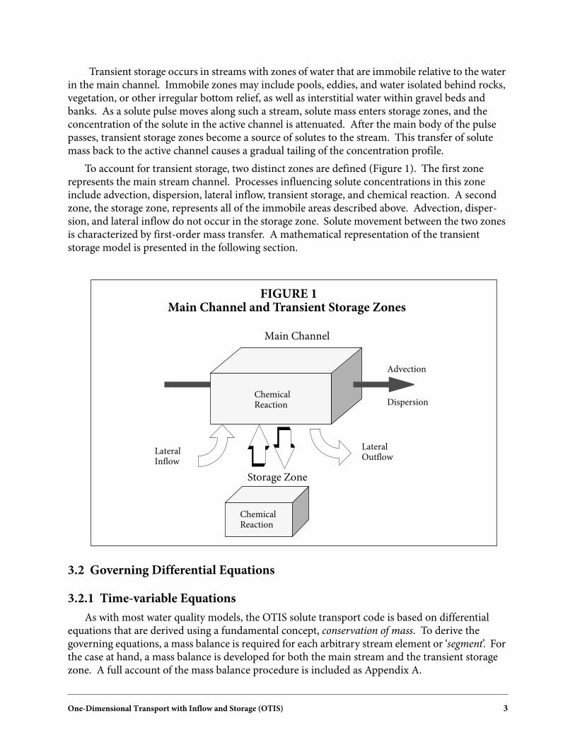
Transient storage occurs in streams with zones of water that are immobile relative to the waterin the main channel. Immobile zones may include pools, eddies, and water isolated behind rocks,vegetation, or other irregular bottom relief, as well as interstitial water within gravel beds andbanks. As a solute pulse moves along such a stream, solute mass enters storage zones, and theconcentration of the solute in the active channel is attenuated. After the main body of the pulsepasses, transient storage zones become a source of solutes to the stream. This transfer of solutemass back to the active channel causes a gradual tailing of the concentration profile.
To account for transient storage, two distinct zones are defined (Figure 1). The first zonerepresents the main stream channel. Processes influencing solute concentrations in this zoneinclude advection, dispersion, lateral inflow, transient storage, and chemical reaction. A secondzone, the storage zone, represents all of the immobile areas described above. Advection, disper-sion, and lateral inflow do not occur in the storage zone. Solute movement between the two zonesis characterized by first-order mass transfer. A mathematical representation of the transientstorage model is presented in the following section.
3.2 Governing Differential Equations
3.2.1 Time-variable Equations
As with most water quality models, the OTIS solute transport code is based on differentialequations that are derived using a fundamental concept, conservation of mass. To derive thegoverning equations, a mass balance is required for each arbitrary stream element or ‘segment’. Forthe case at hand, a mass balance is developed for both the main stream and the transient storagezone. A full account of the mass balance procedure is included as Appendix A.
FIGURE 1Main Channel and Transient Storage Zones
Main Channel
Storage Zone
Advection
Dispersion
LateralOutflow
LateralInflow
ChemicalReaction
ChemicalReaction

4 One-Dimensional Transport with Inflow and Storage (OTIS)
The following table depicts the processes that are considered in the mass balance equations.These processes are assumed to influence solute behavior in the stream channel and/or the storagezone, as indicated below.
Consideration of the above processes in the context of the mass balance gives rise to thecoupled set of differential equations derived in Appendix A. Conservation of mass for the streamand storage-zone segments is given by Equations (1) and (2), respectively:
(1)
(2)
where
A - stream channel cross-sectional area [meters2]
AS - storage zone cross-sectional area [meters2]
C - in-stream solute concentration [mass/meters3]
CL - solute concentration in lateral inflow [mass/meters3]
CS - storage zone solute concentration [mass/meters3]
D - dispersion coefficient [meters2/second]
Advection
Dispersion
Lateral Inflow
Transient Storage
First-Order Decay
ProcessStream
Channel StorageZone
StreamChannel
StorageZoneProcess
TABLE 1Processes Considered
t∂∂C Q
A---
x∂∂C
–1
A---
x∂∂
ADx∂
∂C( )
qLIN
A---------- CL C–( ) α CS C–( ) λC–+ + +=
td
dCS α A
AS
------ C CS–( ) λSCS–=

One-Dimensional Transport with Inflow and Storage (OTIS) 5
Q - volumetric flowrate [meters3/second]
qLIN - lateral inflow rate [meters3/second-meter]
t - time [seconds]
x - distance [meters]
α - storage zone exchange coefficient [/second]
λ - in-stream first-order decay coefficient [/second]
λS - storage zone first-order decay coefficient [/second]
To solve Equations (1) and (2) for the general case where the parameters vary in time andspace, numerical solution techniques must be employed. Numerical techniques for the solution ofthe time-variable equations are the topic of Section 3.4.
3.2.2 Steady-State Equations
The governing differential equations and the corresponding numerical solution techniques canbe greatly simplified if a steady-state solution is desired. Steady-state conditions arise when allloading functions (i.e. boundary conditions) and model parameters are held constant or ‘steady’for an indefinite period of time. Under these conditions, the system eventually reaches an equilib-rium state in which net mass accumulation equals zero.
Setting the accumulation terms (∂C/∂t and dCS/dt) equal to zero, Equations (1) and (2)become:
(3)
(4)
Equation (4), the storage zone equation, is now solved directly for CS, yielding:
(5)
The stream channel equation (Equation (3)), meanwhile, is solved numerically. This solutionis discussed in Section 3.5.
3.3 The Conceptual Stream Channel
To effectively implement a numerical solution scheme, we first define the physical system.Figure 2 depicts an idealized system in which the stream is subdivided into a number of discreteunits or segments. Each of these segments represents a control volume within which mass isconserved. Equations (1) and (2) therefore apply to each segment in the stream network.
0Q
A---
x∂∂C
–1
A---
x∂∂
ADx∂
∂C( )
qLIN
A---------- CL C–( ) α CS C–( ) λC–+ + +=
0 α A
AS
------ C CS–( ) λSCS–=
CSαA
αA λSAS+-------------------------
C=

6 One-Dimensional Transport with Inflow and Storage (OTIS)
Before proceeding to the next section, it is useful to introduce some additional nomenclature.Figure 3 below depicts three arbitrary segments from the stream network shown in Figure 2.Under this segmentation scheme, the subscripts i, i-1, and i+1 denote concentrations and parame-ters at the center of each segment, while the subscripts (i-1,i) and (i,i+1) define values at thesegment interfaces. The length of each segment, ∆x, is also introduced in the figure. These defini-tions are used in Section 3.4 and Appendix B.
Segment1
Segment2
. . .
. . .
. . .
. . .
SegmentN
Q
Segment3
x
qLIN
FIGURE 2Conceptual Watershed
CL
FIGURE 3Segmentation Scheme
Q Segmenti
Segmenti-1
Segmenti+1
Interfacei-1, i
Interfacei, i+1
∆xi-1 ∆xi ∆xi+1
One-Dimensional Transport with Inflow and Storage (OTIS) 7
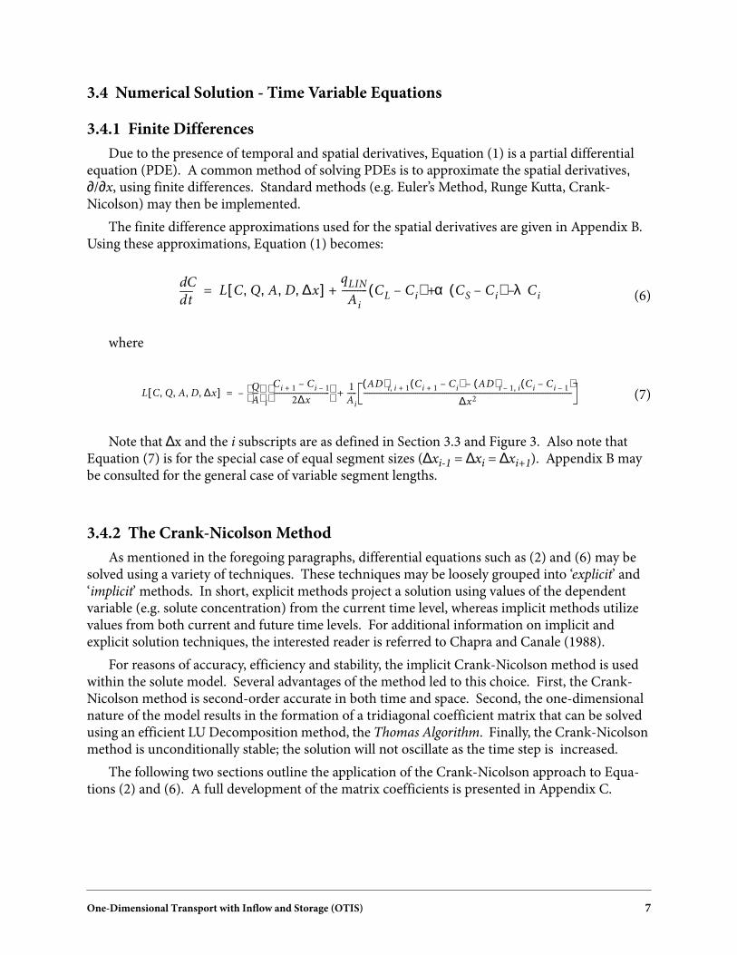
3.4 Numerical Solution - Time Variable Equations
3.4.1 Finite Differences
Due to the presence of temporal and spatial derivatives, Equation (1) is a partial differentialequation (PDE). A common method of solving PDEs is to approximate the spatial derivatives,∂/∂x, using finite differences. Standard methods (e.g. Euler’s Method, Runge Kutta, Crank-Nicolson) may then be implemented.
The finite difference approximations used for the spatial derivatives are given in Appendix B.Using these approximations, Equation (1) becomes:
(6)
where
(7)
Note that ∆x and the i subscripts are as defined in Section 3.3 and Figure 3. Also note thatEquation (7) is for the special case of equal segment sizes (∆xi-1 = ∆xi = ∆xi+1). Appendix B maybe consulted for the general case of variable segment lengths.
3.4.2 The Crank-Nicolson Method
As mentioned in the foregoing paragraphs, differential equations such as (2) and (6) may besolved using a variety of techniques. These techniques may be loosely grouped into ‘explicit’ and‘implicit’ methods. In short, explicit methods project a solution using values of the dependentvariable (e.g. solute concentration) from the current time level, whereas implicit methods utilizevalues from both current and future time levels. For additional information on implicit andexplicit solution techniques, the interested reader is referred to Chapra and Canale (1988).
For reasons of accuracy, efficiency and stability, the implicit Crank-Nicolson method is usedwithin the solute model. Several advantages of the method led to this choice. First, the Crank-Nicolson method is second-order accurate in both time and space. Second, the one-dimensionalnature of the model results in the formation of a tridiagonal coefficient matrix that can be solvedusing an efficient LU Decomposition method, the Thomas Algorithm. Finally, the Crank-Nicolsonmethod is unconditionally stable; the solution will not oscillate as the time step is increased.
The following two sections outline the application of the Crank-Nicolson approach to Equa-tions (2) and (6). A full development of the matrix coefficients is presented in Appendix C.
td
dCL C Q A D ∆x, , , ,[ ]
qLIN
Ai
---------- CL Ci–( ) α CS Ci–( ) λCi–+ +=
L C Q A D ∆x, , , ,[ ] Q
A---
i
Ci 1+ Ci 1––
2∆x-----------------------------
–1
Ai
-----AD( )i i 1+, Ci 1+ Ci–( ) AD( )i 1– i, Ci Ci 1––( )–
∆x2------------------------------------------------------------------------------------------------------------+=

8 One-Dimensional Transport with Inflow and Storage (OTIS)
3.4.3 The Stream Channel
In the Crank-Nicolson algorithm, the right-hand-side of Equation (6) is evaluated at both thecurrent time (time j) and the future time (time j+1). In addition, the time derivative, dC/dt, is esti-mated using a centered difference approximation:
(8)
where
∆t - the integration time step [seconds]
j - denotes the value of a parameter or variable at the current time
j+1 - denotes the value of a parameter or variable at the advanced time
Equation (6) thus becomes:
(9)
where
(10)
Because Equation (9) is dependent on the solute concentrations in the neighboring segmentsat the advanced time level (Ci-1, Ci+1 at time j+1), it is not possible to explicitly solve for Ci
j+1.(Hence we have an ‘implicit’ method.) We can, however, rearrange Equation (9) so that all of theknown quantities appear on the right-hand side and all of the unknown quantities appear on theleft. One exception to this rearrangement in that an unknown quantity, the storage zone concen-tration at the advanced time level (CS
j+1), remains on the right-hand side. This exception isdiscussed in the Section 3.4.5. For now, rearrangement yields:
(11)
This, in turn, may be simplified by grouping terms:
(12)
where
td
dC Cij 1+ Ci
j–
∆t-----------------------=
Cij 1+ Ci
j–
∆t-----------------------
G C CL CS …, , ,[ ] j 1+ G C CL CS …, , ,[ ] j+
2---------------------------------------------------------------------------------------------=
G C CL CS Q A D qLIN ∆x α λ, , , , , , , , ,[ ] L C Q A D ∆x, , , ,[ ]qLIN
Ai
---------- CL Ci–( ) α CS Ci–( ) λCi–+ +=
1∆t
2-----
qLIN
Ai
---------- α λ+ + + Ci
j 1+ ∆t
2-----L C Q A D ∆x, , , ,[ ] j 1+– Ci
j ∆t
2----- G C CL CS etc, , ,[ ] j
qLIN
Ai
----------CLj 1+ αCS
j 1++ + +=
EiCi 1–j 1+ F iCi
j 1+ GiCi 1+j 1++ + Ri=

One-Dimensional Transport with Inflow and Storage (OTIS) 9
(13)
(14)
(15)
(16)
Equations (13) through (16) are for the special case of equal segment sizes. Appendix C maybe consulted for the general case of variable segment lengths.
After developing Equation (12) for all of the segments in the stream network, we arrive at a setof linear algebraic equations. These equations must be solved simultaneously to obtain the in-stream solute concentration, Cj+1, in each of the stream segments. A hypothetical system of equa-tions representing a five-segment network is shown below.
(17)
Systems of equations such as the one shown as Equation (17) may be efficiently solved usingthe Thomas Algorithm. A complete description of the Thomas Algorithm is given in Section 5.4.
3.4.4 The Storage Zone
We now apply the concepts presented in the preceding section to the storage zone equation(Equation (2)). This results in the following Crank-Nicolson equation:
(18)
Ei∆t
2Ai∆x---------------
Qi
2-----
AD( )i 1– i,∆x
-----------------------+ –=
F i 1∆t
2-----
AD( )i 1– i, AD( )i i 1+,+
Ai∆x2-----------------------------------------------------
qLIN
Ai
---------- α λ+ + + +=
Gi∆t
2Ai∆x---------------
Qi
2-----
AD( )i i 1+,∆x
-----------------------– =
Ri Cij ∆t
2----- G C CL CS …, , ,[ ] j
qLIN
Ai
----------CLj 1+ αCS
j 1++ + +=
F1 G1
E2 F2 G2
E3 F3 G3
E4 F4 G4
E5 F5
C1j 1+
C2j 1+
C3j 1+
C4j 1+
C5j 1+
R1
R2
R3
R4
R5
=
CSj 1+ CS
j–
∆t------------------------
α A
AS
------ C CS–( ) λSCS– j 1+
α A
AS
------ C CS–( ) λSCS– j
+
2-------------------------------------------------------------------------------------------------------------------------=

10 One-Dimensional Transport with Inflow and Storage (OTIS)
In contrast to the stream equation, Equation (18) may be solved explicitly for the variable ofinterest, CS
j+1. This yields:
(19)
where
(20)
This explicit formulation is of use in the following section.
3.4.5 Decoupling of the Stream and Storage Zone Equations
At first glance, Equations (12) and (19) appear to be a set of coupled equations due to the pres-ence of an unknown quantity, CS
j+1, on the right-hand side of Equation (12). (Recall from Section3.4.3 that the right-hand side is to contain only known quantities.) This coupling suggests an iter-ative solution technique whereby Equations (12) and (19) are solved in sequence until somedesired level of convergence is obtained. This iterative process is inefficient in that (12) and (19)must be solved more than once for each time step.
Fortunately, these equations can be decoupled by noting the explicit form of Equation (19).Examining (19) we see that the storage concentration is a function of two known quantities, Cj andCS
j, and one unknown quantity, Cj+1. Substituting Equation (19) into Equation (16), we arrive at anew expression for R:
(21)
Although R still contains an unknown quantity, Equation (21) is a much more convenientexpression. The unknown quantity is now Cj+1, a variable that already appears on the left-handside of Equation (12). We can therefore move the term involving Cj+1 to the left side of (12),creating new expressions for F and R:
(22)
(23)
CSj 1+
2 γ– ∆tλS–( )CSj γ C j C j 1++( )+
2 γ ∆tλS+ +----------------------------------------------------------------------------=
γ α∆tA
AS
-------------=
Ri Cij ∆t
2----- G C CL CS …, , ,[ ] j
qLIN
Ai
----------CLj 1+ α
2 γ– ∆tλS–( )CSj γ C j C j 1++( )+
2 γ ∆tλS+ +----------------------------------------------------------------------------
+ + +=
F i 1∆t
2-----
AD( )i 1– i, AD( )i i 1+,+
Ai∆x2-----------------------------------------------------
qLIN
Ai
---------- α 1γ
2 γ ∆tλS+ +----------------------------–
λ+ + + +=
Ri Cij ∆t
2----- G C CL CS …, , ,[ ] j
qLIN
Ai
----------CLj 1+ α
2 γ– ∆tλS–( )CSj γ C j+
2 γ ∆tλS+ +-----------------------------------------------------
+ + +=

One-Dimensional Transport with Inflow and Storage (OTIS) 11
Because R now involves only known quantities, Equation (12) can be solved independently forthe in-stream solute concentration, Cj+1. Having solved (12), the storage zone equation (Equation(19)) becomes a function of three known quantities, CS
j, Cj, and Cj+1. We have thus decoupled thegoverning Crank-Nicolson expressions.
3.5 Numerical Solution - Steady-State Equations
As with the time-variable equations, we approximate the spatial derivatives in Equation (3) viafinite differences. These approximations are given in Appendix B. The resultant algebraic equa-tion for the stream channel is given by:
(24)
The stream channel equation’s dependence on the storage concentration can be eliminated bysubstituting Equation (5) into the above. This yields:
(25)
Since Equation (25) is dependent on the solute concentrations in the neighboring segments(Ci-1, Ci+1), it is not possible to explicitly solve for Ci. We can, however, rearrange Equation (25)so that the unknown quantities, Ci-1, Ci and Ci+1, appear on the left-hand side. This rearrange-ment yields:
(26)
where E, F, G and R are developed in Appendix D. The in-stream solute concentrations aredetermined by solving a system of equations analogous to that shown as Equation (17).
3.6 Boundary Conditions
Two boundary conditions must be specified to solve second-order differential equations suchas Equation (1). For the case of a one-dimensional stream channel, these boundary conditions areapplied at the upstream and downstream boundaries. A thorough discussion of these boundaryconditions is given in Appendix B.
3.6.1 Upstream Boundary Condition
To implement the finite difference scheme described in Appendix B, an upstream boundarycondition must be defined. This condition is shown in Figure 4, where the concentration at theupstream boundary is fixed as Cbc. Note that Cbc is a time-varying forcing function that is set bythe user. User-specification of the upstream boundary condition is discussed in Section 4.5.2.
0 L C Q A D ∆x, , , ,[ ]qLIN
Ai
---------- CL Ci–( ) α CS Ci–( ) λCi–+ +=
0 L C Q A D ∆x, , , ,[ ]qLIN
Ai
---------- CL Ci–( )αλSAS
αA λSAS+-------------------------Ci– λCi–+=
EiCi 1– F iCi GiCi 1++ + Ri=

12 One-Dimensional Transport with Inflow and Storage (OTIS)
3.6.2 Downstream Boundary Condition
In contrast to the upstream condition, the downstream boundary condition is not a fixedconcentration, but rather a fixed dispersive flux. To implement the downstream boundary condi-tion, a dispersive flux is defined at the interface between segments i and i+1. Here the subscript irefers to the last segment in the stream network, while i+1 refers to a fictitious segment adjacent tothe last segment. The dispersive flux is defined as:
(27)
where DSBOUND is a user-supplied value for the dispersive flux. Note that if DSBOUND isset equal to zero, Equation (27) is a zero gradient boundary condition (Arden and Astill, 1970).This implies that the concentration in segment i is equal to that in segment i+1. Due to the poten-tial error introduced by this equality, the modeled stream network should extend well beyond theregion of interest (for example, see Section 6.1).
Application of the downstream boundary condition is shown in Figure 5 and discussed inAppendix B. User-specification of DSBOUND is discussed in Section 4.5.2.
FIGURE 4Segment 1 - Upstream B.C.
flow C1
Cbc C1,2
DC∂x∂
------
i i 1+,
DSBOUND=
FIGURE 5Downstream Boundary Condition
flow Ci-1 Ci Ci+1
DC∂x∂
------
i i 1+,

One-Dimensional Transport with Inflow and Storage (OTIS) 13
4.0 USER’S GUIDE
Now that we have outlined a conceptual basis for the solute transport code, it is time to directour attention to some operational issues. This section provides the details needed to execute theFortran-77 computer program.
4.1 Applicability
Originally developed for use in small mountain streams, the OTIS solute transport model maybe used for any stream or river in which one-dimensional transport can be assumed. As describedby Fischer et al. (1979), one-dimensional analysis is valid for systems in which solute mass isuniformly distributed over the stream’s cross-sectional area. Although absolute uniformity rarelyoccurs in nature, it is a reasonable assumption for streams of small to moderate width and depth.
The model is capable of simulating the transport of conservative substances in one-dimen-sional streams and rivers. Certain non-conservative substances may also be simulated through thespecification of a first-order decay or production rate. The physical processes of advection, disper-sion, lateral inflow and transient storage are explicitly considered in the development of the under-lying mass balance equations.
4.2 Program Features
Several simulation options are available in the solute transport code. These options, describedbelow, allow the model to be used in a flexible manner.
4.2.1 Simulation Modes: Dynamic and Steady-State
The solute transport code may be used to solve either the dynamic equations of Section 3.2.1or the steady-state equations of Section 3.2.2. The following paragraphs describe these two simu-lation modes. A full description of the relevant input parameters is presented in Section 4.5.
The dynamic simulation option is selected when the user is interested in determining the time-variable nature of the transported solute. This option requires the user to specify a time-variableloading function (via the upstream boundary conditions), an integration time step (input variableTSTEP) and a time interval for the printing of results (input variable PSTEP).
As described in Section 3.2.2, the steady-state equations are applicable when the long-termresponse of the system to constant loading conditions is of interest. This steady-state option isinvoked by setting the integration time step, TSTEP, to zero.
4.2.2 Conservative and/or Non-Conservative Substances
Another flexible feature of the code is the ability to model conservative or nonconservativesubstances. Conservative substances are subject to the physical processes of advection, dispersion,lateral inflow and transient storage. One additional process, first-order decay (or production), isconsidered when non-conservative substances are modeled.
To model a conservative substance, the first-order decay coefficients for the main channel andthe storage zones are set to zero. These coefficients, denoted by the input variables LAMBDA andLAMSTOR, are described in Section 4.5.

14 One-Dimensional Transport with Inflow and Storage (OTIS)
Although non-conservative substances may undergo complex chemical, physical and biolog-ical reactions, consideration of these processes is beyond the scope of work described herein.Non-conservative substances are therefore modeled using first-order decay (or production) coeffi-cients. These coefficients represent a one-way loss (gain) of mass from (to) the system.
To simulate a non-conservative substance, the main channel and storage zone input variables,LAMBDA and LAMSTOR, are set accordingly. Positive coefficient values are specified if thesubstance is subject to first-order decay, while negative values are used to specify rates of first-order production. Note that first-order decay coefficients may be calculated using half-life valuesthat are commonly found in the literature:
(28)
where
Λ - first-order decay rate [/second] for the main channel or storage zone
t1/2 - half life [seconds]
4.2.3 Flow Regimes
In addition to the foregoing options, the model has the ability to simulate transport under avariety of flow conditions. This feature is especially significant, because an accurate simulationrelies on a realistic description of the hydrologic flow regime. To this end, the model considersspatially (uniform/non-uniform) and temporally (steady/unsteady) varying flows. For a review ofthe various flow regimes, the reader is referred to Henderson (1966).
User specification of the governing hydrologic regime is summarized in the table below. Thefirst two options shown in the table are relatively straightforward as they involve a steady flowregime. Under this regime, model parameters such as lateral inflow and cross-sectional arearemain constant with respect to time. This ‘steadiness’ results in a fairly simple set of user inputfiles.
In contrast to steady flow, the third option in Table 2, unsteady flow, involves model parame-ters that vary in time. This option is typically selected when the solute model is used in conjunc-tion with a watershed-scale hydraulic routing model. Such a routing model would provide time-varying lateral inflows, channel flowrates and cross-sectional areas for use as input to the solutemodel. The input format used to couple the two models is given in Section 4.5.5.
Λ 0.693
t1 2⁄------------=

One-Dimensional Transport with Inflow and Storage (OTIS) 15
4.3 Conceptual Stream Channel, Revisited
Before giving a detailed description of the model’s input requirements, it is useful to definesome of the program variables in terms of the conceptual watershed. In the text that follows, alluser-supplied input parameters are printed using uppercase characters.
Figure 6 depicts the stream network as a series of reaches. For our purposes, a reach is definedas a continuous distance along which model parameters remain constant. A reach, for example,will have a spatially constant dispersion coefficient, decay rate and lateral inflow rate. The numberof reaches defined for a given system reflects both its inherent variability and the availability ofdata. A spatially uniform stream may be modeled using a single reach, while a stream with a well-characterized variation in channel properties may be simulated using several reaches. The numberof reaches in the modeled system is specified by the NREACH input parameter.
Each reach is subdivided into a number of computational elements or segments. Each segmentrepresents a control-volume over which the governing mass-balance equations apply. For a givenreach, there are NSEG segments of length DELTAX. Note that DELTAX is determined from thereach length, RCHLEN, and the number of segments:
(29)
Steady, Uniform Flow
Steady, Non-Uniform Flow
Unsteady, Non-Uniform Flow
Set the lateral flow terms, QLATIN andQLATOUT, to zero. Also set the change inflow indicator, QSTEP, to zero.
Set the lateral inflow terms, QLATIN andQLATOUT, to the desired values. Set thechange in flow indicator, QSTEP, to zero.
Prepare the flow file using flow, lateral inflowand area data that are generated by a suitablerouting model (e.g. DR3M). Set the changein flow indicator, QSTEP, equal to the outputtime step of the routing model.
Flow Regime User Specifications
TABLE 2Flow Regimes
DELTAXRCHLEN
NSEG-----------------------=

16 One-Dimensional Transport with Inflow and Storage (OTIS)
Additional program variables are shown in Figure 7. Here we see the first reach in the streamnetwork and its relationship to some of the required input variables. Because this reach begins atthe upstream boundary of the system, we define an incoming flowrate, QSTART, and its associatedsolute concentration, USCONC. USCONC is the upstream boundary condition, Cbc, discussed inSection 3.6.1. The program variable denoting the starting stream distance, XSTART, also applies atthe upstream end of reach one. Note that these three variables apply only to the first reach of thestream network.
The remaining program variables shown in the figure, QLATIN, CLATIN and QLATOUT, arespecified for each reach in the modeled system (note that for unsteady flows, these variables maynot necessarily correspond to specific reaches - see Section 4.5.5). The lateral inflow rate,QLATIN, represents the flow entering the channel via overland flow, interflow and groundwaterdischarge. This additional flow carries a solute concentration, CLATIN. The final variable,QLATOUT, is a lateral outflow term representing a loss of water from the stream channel. BothQLATIN and QLATOUT are specified on a per unit length basis (i.e. in meters3/second-meter).
Reach Reach. . .
Reach. . .
Reach
Segment Segment. . .
Segment. . .
Segment
Reach j
. . . NREACH
NSEGji21
1 2 j
FIGURE 6Conceptual Watershed - Reaches and Segments
RCHLENj
DELTAXj

One-Dimensional Transport with Inflow and Storage (OTIS) 17
4.4 Input/Output Structure
4.4.1 Input Files
The input/output structure of the solute transport code is depicted in Figure 8. Three inputfiles are used to specify model parameters, print options and simulation control variables. A briefdescription of each of these files is given here. For a full description of the input files and programvariables, see Section 4.5.
The first input file, ‘control.inp’, specifies the number of simulations, the filenames of theremaining input files and the names of the output files. Unlike the other input filenames,‘control.inp’ is hardcoded; its name cannot be set by the user. It is important to note that the speci-fication of filenames under the UNIX operating system is case specific, i.e. there is a differencebetween upper and lower case characters. The filename, ‘CONTROL.INP’, for example, is notequivalent to ‘control.inp’.
A second input file, the parameter file, sets simulation options, boundary conditions andmodel parameters that remain constant throughout the run. The final input file, the flow file,contains model parameters that could potentially vary during the course of the simulation (e.g.volumetric flowrate, stream cross-sectional area). The filenames of the parameter and flow filesare specified by the user in the control file, control.inp.
FIGURE 7Conceptual Watershed - Reach 1
QSTART1 2 3
x = XSTART
QLATIN
USCONC
CLATIN
QLATOUT
. . . . . . . NSEG1

18 One-Dimensional Transport with Inflow and Storage (OTIS)
4.4.2 Output Files
Also shown in Figure 8 are the output files created by the solute transport code. Upon comple-tion of a model run, the file ‘echo.out’ contains a listing of (“echo of ”) all of the user-specified simu-lation options and model parameters. This file also contains any error messages generated duringprogram execution. A sample listing of echo.out is given in Appendix E.
In addition to the echo file, the model creates one output file for each solute. These soluteoutput files contain a time-series of solute concentrations at various locations along the stream.The filenames of the output files are specified in control.inp.
4.5 Input Format
Three input files must be assembled prior to program execution. In the sections that follow,each input file is described in terms of a set of ‘record types’. Within each of these record types, oneor more ‘fields’ is used to specify various input parameters. In general, record types refer to lines inthe input file, while fields correspond to specific columns within each record.
After describing the record types, a sample input file is given. These sample files show thebasic structure of each input data set. Of particular interest is the way in which some record typesare used repeatedly within a given input file. The sample files given herein are for a dynamic simu-lation of two conservative substances in a hypothetical three-reach system.
FIGURE 8Input/Output Diagram
OTIS
control.inp echo.out
flowfile
parameterfile solute output files
(one file per solute)

One-Dimensional Transport with Inflow and Storage (OTIS) 19
4.5.1 The Control File
The control file, control.inp, is used to specify the number of model runs and the filenames forthe various input and output files. As shown in Table 3, the control file contains four distinctrecord types.
Record Type 1 - The Number of Runs
For a given execution of the program, the underlying simulation model may be executed morethan once. For example, the user may wish to run the model using two different parameter files.This would be accomplished by placing the integer value ‘2’ in one of the first five columns ofrecord type 1.
The number of model runs, NRUNS, is set using record 1. Note that for NRUNS > 1, multipleinput and output files must be specified by repeating the block of record types 2-4 for each modelrun.
Record Types 2-4 - Input and Output Filenames
Records 2-4 specify filenames for the input and output files. The filename for the parameterfile is set using record type 2, while record type 3 specifies the name of the flow file. Finally, recordtype 4 specifies the names of the solute output files.
1
2*
4*
3*
NRUNS
FILE
QFILE
FILES
I
C
C
C
1-5
1-20
1-20
1-20
Number of Runs
Filename for the Parameter File
Filenames for the Solute Output Files
Filename for the Flow File
RecordType
ProgramVariable Format Col. Description
TABLE 3The Control File
I - IntegerC - Character
*Notes: 1) Repeat Record Type 4 for each solute modeled
2) Repeat the block of Record Types 2-4 for each model run, i.e. types 2-4 are first specified for run one, followed by types 2-4 for run two, etc.

20 One-Dimensional Transport with Inflow and Storage (OTIS)
Although Table 3 lists four record types, the control file often contains more than four records,as some of the record types may be repeated. Record type 4, for example, is repeated for eachsolute (an output file is created for each solute). Furthermore, record types 2-4 are repeated foreach model run (when NRUNS > 1).
Sample Control File
A sample control file is shown below. In this example, two model runs are requested (RecordType 1). For the first run, the parameter and flow files are named, ‘params1.inp’ and ‘flow.inp’,respectively (Record Types 2 and 3); the two output files are dubbed ‘solute1a.out’ and‘solute2a.out’ (Record Type 4, repeated). For the second run, there is a different parameter file(params2.inp) but the same flow file; output is directed to the files solute1b.out and solute2b.out.
4.5.2 The Parameter File
The parameter file specifies print options, boundary conditions and the model parameters thatremain constant throughout the run. The format of the parameter file is given in Tables 4-7. Theparameter file is created using the 17 record types discussed below.
Record Type 1 - Simulation Title
The first record in the parameter file is a simulation title of up to 80-characters. This title isprinted as part of the echo output file.
Record Types 2 & 3 - Print Parameters
The print option and the print step are set using record types 2 and 3. Record type 2 indicatesthe hydrologic region of interest. If a value or ‘1’ is entered, results are printed for the mainchannel only. Results for both the main channel and the storage zone are printed if a ‘2’ is entered.
Following the specification of the print option, record type 3 sets the time interval at whichresults are printed, the print step. If, for example, results are needed every 15 minutes, a value of0.25 hours is entered for the print step. The actual print step and the requested print step maydiffer if the requested step is not an even multiple of the integration time step. In this case, theprogram internally sets the print step equal to the nearest multiple of the integration time step.
FIGURE 9Sample Control File
params2.inpflow.inpsolute1b.outsolute2b.out
2params1.inpflow.inpsolute1a.outsolute2a.out

One-Dimensional Transport with Inflow and Storage (OTIS) 21
Record Types 4-6 - Time Parameters
The next step in constructing the parameter file is to enter the appropriate time parameters.The first such parameter, the integration time step (TSTEP), is set in record type 4. Great careshould be taken when setting the integration time step for the Crank-Nicolson solution procedure(See Section 3.4). Multiple model runs may be required to determine a time step that yields anaccurate solution. As discussed in Section 4.2.1, the model’s steady-state solution scheme isemployed if TSTEP is set to zero. The time-variable equations are solved when TSTEP is greaterthan zero.
The remaining time parameters, TSTART and TFINAL, are set via record types 5 and 6. Theinput variable TSTART denotes the simulation start time, while TFINAL specifies the end of thesimulation.
Record Type 7 - Distance at the Upstream Boundary
The input parameter XSTART indicates the distance at the upstream boundary of the streamnetwork. This distance is relative to an arbitrary one-dimensional coordinate system. Duringprogram execution, XSTART is utilized to calculate the distances at various locations downstream.As the upstream boundary is at the beginning of the modeled area, XSTART is commonly set to0.0 meters.
Record Type 8 - Downstream Boundary Condition
A downstream boundary condition, DSBOUND, is set using record type 8. In many modelingapplications, the flux represented by the boundary condition is set to zero. The user should,however, ensure that the location of the boundary is sufficiently downstream from the nearestlocation of interest. A more complete description of the downstream boundary condition is givenin Section 3.6 and Appendix B.
Record Type 9 - The Number of Reaches
As discussed in Section 4.3, the stream channel is divided into a number of reaches, NREACH.This parameter is set by record type 9. For each reach, spatially constant parameters are specifiedusing record type 10.

22 One-Dimensional Transport with Inflow and Storage (OTIS)
Record Type 10 - Reach Specific Parameters
This record type sets the parameters for each reach (Table 5). Unlike record types 1-9, recordtype 10 contains more than one program variable. The first field in the record indicates thenumber of segments located within the reach, NSEG. A second field specifies the length of thereach, RCHLEN. It is important to note that these two parameters define the length of eachsegment, DELTAX (see Section 4.3).
A third field in this record type is the dispersion coefficient, DISP. The storage zone cross-sectional area, AREASTOR, and the storage zone exchange coefficient, ALPHA, complete recordtype 10. Because this record type is used for the reach specific parameters, it is repeated NREACHtimes, i.e. once for each reach in the stream network.
1
2
4
3
TITLE
PRTOPT
PSTEP
TSTEP
C
I
D
D
1-80
1-5
1-13
1-13
Simulation Title
Print Option
Integration Time Step
Print Step
RecordType
ProgramVariable Format Col. Description
TABLE 4The Parameter File - Record Types 1-9
I - IntegerC - Character
5
6
8
7
TSTART
TFINAL
XSTART
DSBOUND
D
D
D
D
1-13
1-13
1-13
1-13
Simulation Starting Time
Simulation Ending Time
Downstream Boundary Condition
Distance at the Upstream Boundary
---
---
hours
hours
hour
hour
meters
mass/m2-sec
D - Double Precision
9 NREACH I 1-5 Number of Stream Reaches---
Units

One-Dimensional Transport with Inflow and Storage (OTIS) 23
Record Types 11-13 - Solute Specific Parameters
The number of solutes to model, NSOLUTE, is given by record type 11 (Table 6). For eachsolute, it is possible to specify a first-order decay rate in each reach for both the main channel andthe storage zone. The main channel decay coefficient, LAMBDA, is set in record type 12, whiletype 13 is used for the storage zone decay coefficient, LAMSTOR.
The specification of record types 12 and 13 depends on the number of solutes and the numberof reaches. The decay coefficients for reach one are first set using record types 12 and 13. Withineach of these record types, the decay field is repeated horizontally for each solute, i.e. the coeffi-cient for solute one appears in columns 1-13, the coefficient for solute two appears in columns 14-26, etcetera. After specifying LAMBDA and LAMSTOR for each solute in reach one, record types12 and 13 are repeated vertically for reach two. This repetition continues until the decay coeffi-cients are set for all of the reaches. In general, there are NREACH blocks of record types 12 and13. Each record contains NSOLUTE fields that are 13 characters wide.
NSEG
RCHLEN
DISP
AREASTOR
I
D
D
D
1-5
6-18
32-44
19-31
Number of Segments in Reach j
Length of Reach j
Storage Zone Area for Reach j
Dispersion Coefficient for Reach j
ProgramVariable Format Col. Description
ALPHA D 45-57 Storage Zone Exchange Coefficient
---
meters
meters2/sec
meters2
/second
Units
TABLE 5The Parameter File - Record Type 10
I - IntegerD - Double Precision
Note: Record Type 10 is repeated once for each reach in the stream network (it repeats ‘NREACH’ times)

24 One-Dimensional Transport with Inflow and Storage (OTIS)
Record Types 14 & 15 - Print Locations
While record types 2 and 3 deal with the timing and type of printed output, record types 14and 15 control the locations at which results are printed. The flexible approach described hereallows the user to request solute concentrations at a number of locations along the stream. Recordtype 14 specifies the number of print locations, NPRINT, while record type 15 declares thedistance, in meters, of a given print location (PRTLOC). Record type 15 is repeated NPRINTtimes. Note that XSTART (record type 7) and PRTLOC must use the same coordinate system.
Record Types 16 & 17 - Upstream Boundary Conditions
The final record types in the parameter file specify the upstream boundary conditions. Asshown in Table 6, the number of boundary conditions, NBOUND, is set using record type 16. Ingeneral, NBOUND equals the number of values for the upstream boundary concentration. Notethat NBOUND should be set to one for a steady-state simulation.
11
12*
14
13*
NSOLUTE
LAMBDA
LAMSTOR
NPRINT
I
D
I
D
1-5
1-13*
1-5
1-13*
Number of Solutes
In-stream First-Order Decay Rate
Number of Print Locations
Storage Zone First-Order Decay Rate
RecordType
ProgramVariable Format Col. Description
TABLE 6The Parameter File - Record Types 11-16
15*
16
PRTLOC
NBOUND
D
I
1-13
1-5
Print Location
Number of Boundary Conditions
---
/second
/second
---
meters
---
Units
I - IntegerD - Double Precision
*Notes: 1) If there is more than one solute, Record Types 12 and 13 repeat horizontally, i.e. the decay
rate for solute one is placed in columns 1-13, the rate for solute 2 is placed in columns 14-26, etc.
2) Record Types 12 and 13 repeat for each reach in the stream network. Note that Records 12 and 13 are first given for reach one, followed by Records 12 and 13 for reach two, etc.
3) Record Type 15 repeats for each print location (it repeats ‘NPRINT’ times).
One-Dimensional Transport with Inflow and Storage (OTIS) 25
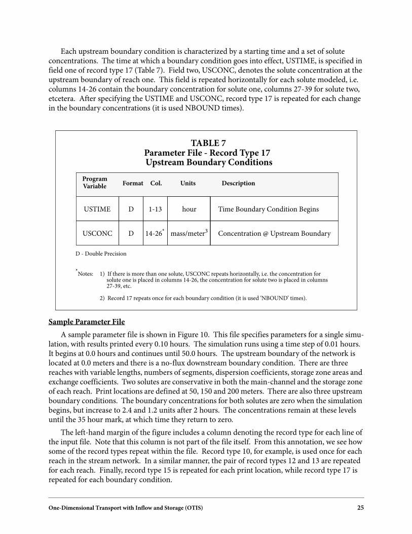
Each upstream boundary condition is characterized by a starting time and a set of soluteconcentrations. The time at which a boundary condition goes into effect, USTIME, is specified infield one of record type 17 (Table 7). Field two, USCONC, denotes the solute concentration at theupstream boundary of reach one. This field is repeated horizontally for each solute modeled, i.e.columns 14-26 contain the boundary concentration for solute one, columns 27-39 for solute two,etcetera. After specifying the USTIME and USCONC, record type 17 is repeated for each changein the boundary concentrations (it is used NBOUND times).
Sample Parameter File
A sample parameter file is shown in Figure 10. This file specifies parameters for a single simu-lation, with results printed every 0.10 hours. The simulation runs using a time step of 0.01 hours.It begins at 0.0 hours and continues until 50.0 hours. The upstream boundary of the network islocated at 0.0 meters and there is a no-flux downstream boundary condition. There are threereaches with variable lengths, numbers of segments, dispersion coefficients, storage zone areas andexchange coefficients. Two solutes are conservative in both the main-channel and the storage zoneof each reach. Print locations are defined at 50, 150 and 200 meters. There are also three upstreamboundary conditions. The boundary concentrations for both solutes are zero when the simulationbegins, but increase to 2.4 and 1.2 units after 2 hours. The concentrations remain at these levelsuntil the 35 hour mark, at which time they return to zero.
The left-hand margin of the figure includes a column denoting the record type for each line ofthe input file. Note that this column is not part of the file itself. From this annotation, we see howsome of the record types repeat within the file. Record type 10, for example, is used once for eachreach in the stream network. In a similar manner, the pair of record types 12 and 13 are repeatedfor each reach. Finally, record type 15 is repeated for each print location, while record type 17 isrepeated for each boundary condition.
USTIME
USCONC
D
D
1-13
14-26*
Time Boundary Condition Begins
Concentration @ Upstream Boundary
ProgramVariable Format Col. Description
hour
mass/meter3
Units
TABLE 7Parameter File - Record Type 17
D - Double Precision
Upstream Boundary Conditions
*Notes: 1) If there is more than one solute, USCONC repeats horizontally, i.e. the concentration for
solute one is placed in columns 14-26, the concentration for solute two is placed in columns 27-39, etc.
2) Record 17 repeats once for each boundary condition (it is used ‘NBOUND’ times).

26 One-Dimensional Transport with Inflow and Storage (OTIS)
4.5.3 The Flow File
As previously discussed, the flow file defines the model parameters that can potentially vary intime. These parameters include the volumetric flowrate (Q and QSTART), lateral flow rates(QLATIN and QLATOUT), stream cross-sectional area (AREA), and solute concentrations associ-ated with the lateral inflows (CLATIN). Collectively, these parameters are known as the flow vari-ables.
The format of the flow file depends on the nature of the parameters contained therein. If all ofthe flow variables are constant with respect to time, the flow is ‘steady’, and the format given inSection 4.5.4 is used. If any of the flow variables change in time, the flow regime is considered‘unsteady’ and the format is as described in Section 4.5.5.
FIGURE 10Sample Parameter File
RecordType
sample input file - 3 reaches, 2 solutes10.100.010.0050.00.00.0325 50.00 0.02 0.05 3.0E-550 100.0 0.05 0.06 3.0E-5100 200.0 0.05 0.06 5.0E-520.0 0.00.0 0.00.0 0.00.0 0.00.0 0.00.0 0.0350.0150.0200.030.0 0.0 0.02.0 2.4 1.235.0 0.0 0.0
1 2 3 4 5 6 7 8 9101010111213121312131415151516171717

One-Dimensional Transport with Inflow and Storage (OTIS) 27
Note that for steady flow conditions, the flow variables are specified on a reach by reach basis.When the flow regime is unsteady, the flow variables are specified using flow locations. Thisdistinction is shown in the following sections.
4.5.4 The Flow File - Steady Flow
When the flow variables are constant with respect to time, the ‘steady’ flow option is invoked.As shown in the following sections, the specification of a steady flow file is fairly straightforward.
Record Type 1 - Change-in-Flow Indicator
The first record type in the flow file is the change-in-flow indicator, QSTEP. This record typeis used to define the flow regime. As shown in Table 8, QSTEP is the time interval betweenchanges in the flow variables. Here we are concerned with a steady flow regime in which the flowvariables are constant. In this case, QSTEP is simply set to zero.
Record Types 2 & 3 - Flow Variables
The remaining record types for a steady flow file are as described in Tables 9 and 10. Recordtype 2 sets the volumetric flowrate at the upstream boundary, QSTART. The remaining flow vari-ables are set using record type 3. As shown in Table 10, the first three fields of this record specifythe lateral flow rates (QLATIN and QLATOUT) and the cross-sectional area (AREA) for a partic-ular reach. The fourth field, used to indicate the solute concentration of the lateral inflows(CLATIN), repeats horizontally for each solute modeled. Since the flow variables vary from reachto reach, record type 3 must be repeated for each reach in the network.
QSTEP D 1-13 Change-in-Flow Indicator (set to zero)
ProgramVariable Format Col. Description
hour
Units
TABLE 8Steady Flow File - Record Type 1
D - Double Precision
QSTART D 1-13 Flowrate at the Upstream Boundary
ProgramVariable Format Col. Description
meters3/sec
Units
TABLE 9Steady Flow File - Record Type 2
D - Double Precision

28 One-Dimensional Transport with Inflow and Storage (OTIS)
Sample Flow File - Steady Flow
A sample flow file for a steady flow regime is shown in Figure 11. In this example, the volu-metric flow rate at the upstream boundary is fixed using record type 2. Lateral inflow occurs inreaches 2 and 3, but the inflow concentrations for both solutes equal zero. Cross-sectional areasincrease from reach to reach. This flow file is for a hypothetical three-reach system.
QLATIN
QLATOUT
AREA
CLATIN*
D
D
D
D
1-13
14-26
40-52*
27-39
Lateral Inflow Rate for Reach j
Lateral Outflow Rate for Reach j
Concentration of Lateral Inflow
Stream Channel Area for Reach j
ProgramVariable Format Col. Description
m3/sec-m
m3/sec-m
meters2
mass/meters3
Units
TABLE 10Steady Flow File - Record Type 3
D - Double Precision
*Notes: 1) If there is more than one solute, CLATIN repeats horizontally, i.e. the lateral inflow
concentration for solute one is placed in columns 40-52, the concentration for solute two is placed in columns 53-65, etc.
2) Record type 3 repeats once for each reach in the stream network.
FIGURE 11Sample Steady Flow File
0.00 1
RecordType
6.10E-3 20.00 0.00 0.20 0.00 0.003.10E-6 0.00 0.25 0.00 0.001.65E-4 0.00 0.35 0.00 0.00
3 3 3
One-Dimensional Transport with Inflow and Storage (OTIS) 29
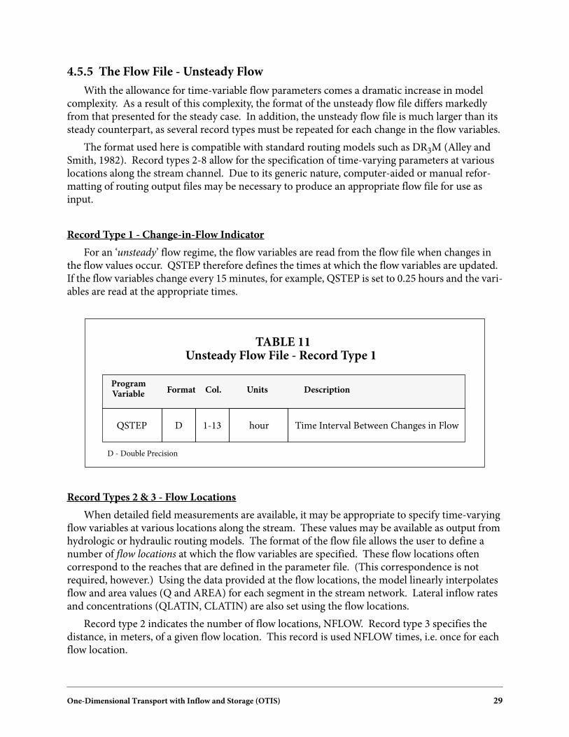
4.5.5 The Flow File - Unsteady Flow
With the allowance for time-variable flow parameters comes a dramatic increase in modelcomplexity. As a result of this complexity, the format of the unsteady flow file differs markedlyfrom that presented for the steady case. In addition, the unsteady flow file is much larger than itssteady counterpart, as several record types must be repeated for each change in the flow variables.
The format used here is compatible with standard routing models such as DR3M (Alley andSmith, 1982). Record types 2-8 allow for the specification of time-varying parameters at variouslocations along the stream channel. Due to its generic nature, computer-aided or manual refor-matting of routing output files may be necessary to produce an appropriate flow file for use asinput.
Record Type 1 - Change-in-Flow Indicator
For an ‘unsteady’ flow regime, the flow variables are read from the flow file when changes inthe flow values occur. QSTEP therefore defines the times at which the flow variables are updated.If the flow variables change every 15 minutes, for example, QSTEP is set to 0.25 hours and the vari-ables are read at the appropriate times.
Record Types 2 & 3 - Flow Locations
When detailed field measurements are available, it may be appropriate to specify time-varyingflow variables at various locations along the stream. These values may be available as output fromhydrologic or hydraulic routing models. The format of the flow file allows the user to define anumber of flow locations at which the flow variables are specified. These flow locations oftencorrespond to the reaches that are defined in the parameter file. (This correspondence is notrequired, however.) Using the data provided at the flow locations, the model linearly interpolatesflow and area values (Q and AREA) for each segment in the stream network. Lateral inflow ratesand concentrations (QLATIN, CLATIN) are also set using the flow locations.
Record type 2 indicates the number of flow locations, NFLOW. Record type 3 specifies thedistance, in meters, of a given flow location. This record is used NFLOW times, i.e. once for eachflow location.
QSTEP D 1-13 Time Interval Between Changes in Flow
ProgramVariable Format Col. Description
hour
Units
TABLE 11Unsteady Flow File - Record Type 1
D - Double Precision

30 One-Dimensional Transport with Inflow and Storage (OTIS)
Several requirements must be kept in mind when specifying flow locations. The requirements,listed below, are checked internally by the computer code:
• The flow locations must be entered in ascending (downstream) order, i.e. the second loca-tion must be downstream from the first, the third must be downstream from the second,etcetera.
• The first flow location must be placed at the upstream end of the stream network. Thisimplies that FLOWLOC1 equals XSTART, where XSTART is the starting location specifiedin the parameter file. Note that the flow specified at this first location is analogous to theQSTART parameter in the steady flow file.
• The last flow location must be placed at or below the downstream boundary.
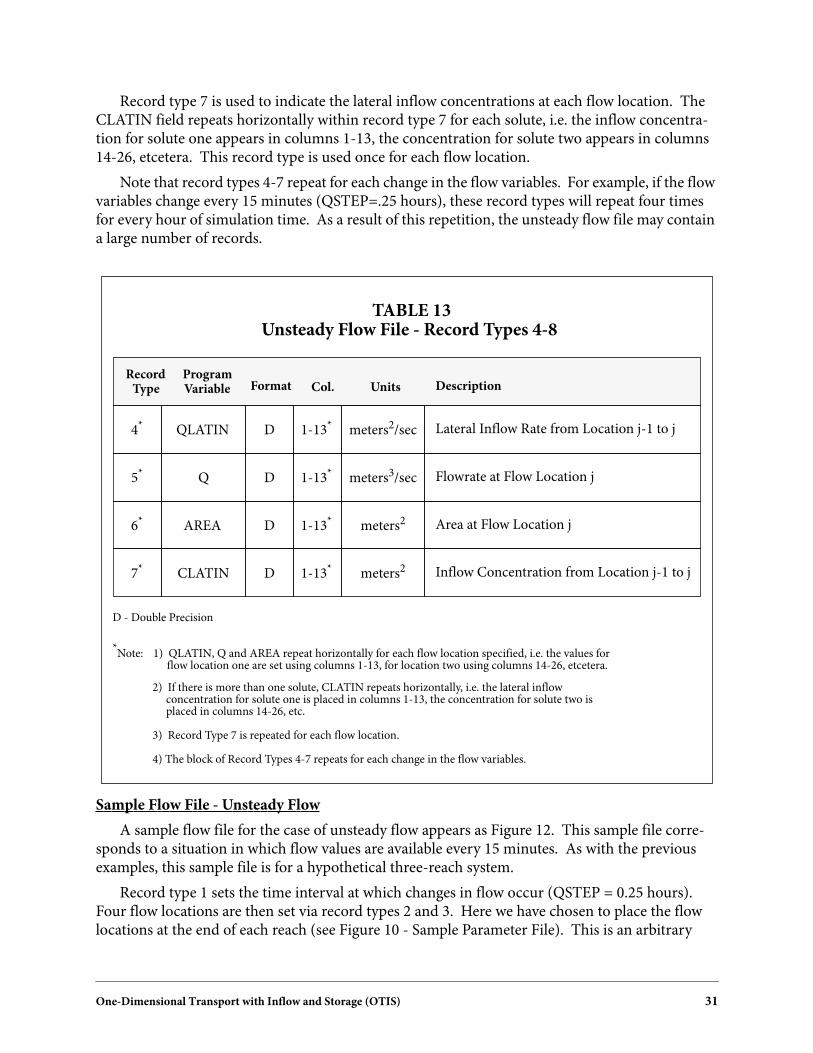
Record Type 4-7 - Lateral Flows, Flows and Areas
In contrast to the steady flow file, lateral flows and concentrations (QLATIN, CLATIN) do notnecessarily correspond to specific reaches. In the unsteady flow file, these parameters are specifiedfor each flow location. The value specified is used for all segments in-between the current flowlocation and the flow location immediately upstream (from location j-1 to location j). Note thatthis scheme corresponds to that for the steady flow file if the flow locations are placed at the end ofeach reach. As stated earlier, the flow and area (Q and AREA) values at the flow locations are usedto interpolate values for the segments within the network.
Lateral inflow, flow and area values are set for each flow location using record types 4-6,respectively. As shown in Table 13, the input fields in these record types (QLATIN, Q and AREA)repeat horizontally for each flow location. The values for flow location one appear in columns 1-13, while the those for flow location two appear in columns 14-26, etcetera.
2 NFLOW I 1-5 Number of Flow Locations
RecordType
ProgramVariable
Format Col. Description
TABLE 12Unsteady Flow File - Record Types 2 & 3
3* FLOWLOC D 1-13 Flow Location
---
meters
Units
I - IntegerD - Double Precision
*Note: Record Type 3 repeats for each flow location (it repeats ‘NFLOW’ times).
One-Dimensional Transport with Inflow and Storage (OTIS) 31
Record type 7 is used to indicate the lateral inflow concentrations at each flow location. TheCLATIN field repeats horizontally within record type 7 for each solute, i.e. the inflow concentra-tion for solute one appears in columns 1-13, the concentration for solute two appears in columns14-26, etcetera. This record type is used once for each flow location.
Note that record types 4-7 repeat for each change in the flow variables. For example, if the flowvariables change every 15 minutes (QSTEP=.25 hours), these record types will repeat four timesfor every hour of simulation time. As a result of this repetition, the unsteady flow file may containa large number of records.
Sample Flow File - Unsteady Flow
A sample flow file for the case of unsteady flow appears as Figure 12. This sample file corre-sponds to a situation in which flow values are available every 15 minutes. As with the previousexamples, this sample file is for a hypothetical three-reach system.
Record type 1 sets the time interval at which changes in flow occur (QSTEP = 0.25 hours).Four flow locations are then set via record types 2 and 3. Here we have chosen to place the flowlocations at the end of each reach (see Figure 10 - Sample Parameter File). This is an arbitrary
4* QLATIN D 1-13* Lateral Inflow Rate from Location j-1 to j
RecordType
ProgramVariable Format Col. Description
TABLE 13Unsteady Flow File - Record Types 4-8
meters2/sec
Units
D - Double Precision
*Note: 1) QLATIN, Q and AREA repeat horizontally for each flow location specified, i.e. the values for
flow location one are set using columns 1-13, for location two using columns 14-26, etcetera.
5* Q D 1-13* Flowrate at Flow Location j
6* AREA D 1-13* Area at Flow Location j
meters3/sec
meters2
7* CLATIN D 1-13* Inflow Concentration from Location j-1 to jmeters2
2) If there is more than one solute, CLATIN repeats horizontally, i.e. the lateral inflow concentration for solute one is placed in columns 1-13, the concentration for solute two is placed in columns 14-26, etc.
3) Record Type 7 is repeated for each flow location.
4) The block of Record Types 4-7 repeats for each change in the flow variables.

32 One-Dimensional Transport with Inflow and Storage (OTIS)
choice of locations, since the flow locations need not correspond to the reach end points. Notethat the flow locations appear in ascending or downstream order, with the first location at theupstream end of the stream network.
After defining the flow locations, record type 4 is used to set the lateral inflow rate. Channelflow and cross-sectional areas for each flow location are set by record types 5 and 6, respectively.Record type 7 is used repeatedly to specify the solute concentrations in the lateral inflows.Although not shown in the figure, record types 4-7 are repeated for every 0.25 hours (i.e. QSTEP)of simulation time.
4.6 The Post-Processor
A simple post-processor is available for use with the OTIS solute transport code. This postpro-cessor reformats the solute output files so that they may be plotted using the Xgraph plotting utility(Harrison, 1989).
FIGURE 12Sample Unsteady Flow File
0.25 1
RecordType
4 20.0050.0150.0
3 3 3
350.0 3 4 0.00e-0 0.00e-0 3.10e-6 1.65e-4 5 6
6.10e-3 6.10e-3 6.41e-3 3.94e-20.20 0.20 0.25 0.35
(Records 4-7 repeat for each change in flow)
7 7 7 7
0.00 0.000.00 0.000.00 0.000.00 0.00
4 5 6 7 7 7 7 . . . .

One-Dimensional Transport with Inflow and Storage (OTIS) 33
5.0 PROGRAMMER’S GUIDE
This section provides an overview of the solute transport computer code. Of special impor-tance are the following topics:
• Simple User Modifications - Maximum Dimensions (Section 5.2.1)
• Computational Efficiency (Section 5.4)
• Program Installation (Section 5.6)
5.1 Model Development
The OTIS computer code is written in ANSI Fortran-77. This code is loosely based on anearlier program by Bencala and Walters (1990). Software development was conducted on a SUN4workstation under the UNIX operating system (SunOS 4.0.3). The model has also been compiledand tested on a Data General Aviion workstation.
Although primarily intended for UNIX-based platforms, the code can be adapted for otheroperating systems such as PRIMOS, VMS or DOS. Minor program modifications may be neces-sary for these systems.
5.2 Include Files
As described in Section 5.7, the code consists of several small subroutines. To facilitateprogram modification, two ‘Include’ files are used. By using include files, key program informa-tion may be shared between subroutines. This information may be modified by editing theinclude files rather than each of the individual routines.
5.2.1 Maximum Dimensions - fmodules.inc
One of the shortcomings of the Fortran computer language is the static allocation of memory.Under this allocation scheme, the size or ‘dimension’ of each vector and array must be fixed prior toprogram execution. This requires some a priori knowledge of the maximum dimension for eachmodel parameter. Selection of an appropriate size for each parameter is a difficult task, as exces-sively small values limit program applicability, while excessively large values waste programmemory.
To minimize this shortcoming, the maximum dimensions for the entire model are defined in asingle include file, ‘fmodules.inc’. Increases or decreases in the maximum dimensions are made byediting the include file and compiling the model as described in Section 5.6.
The default values for the maximum dimensions are shown in Table 14. In general, each ofthese dimensions corresponds to a user-supplied input variable. This correspondence is shownparenthetically in the third column of the table.
When running the model, the input variables may not exceed the maximum values. Thenumber of print locations (see Section 4.5.2 - Record Type 14), for example, may not exceed themaximum value given by MAXPRINT. When an input value exceeds its given maximum,program execution is terminated and a error message is issued. At this point the user mustincrease the appropriate maximum (by editing fmodules.inc) and re-compile the program.

34 One-Dimensional Transport with Inflow and Storage (OTIS)
5.2.2 Logical Devices - lda.inc
In the Fortran computer language, a unit number is assigned to each file used for input and/oroutput. These unit numbers, also known as logical device assignments (ldas), must be specifiedfor each read and write operation. Program variables used to store the unit numbers are sharedbetween the input and output subroutines using a Fortran Common block. This common block isdefined in the include file lda.inc.
5.3 Error Checking
The program’s input subroutines perform several tests to validate the input data. If errors aredetected, an error message is issued and program execution is terminated. The error checkingcapabilities of the model are as follows:
• The number of reaches, NREACH, must not exceed the maximum, MAXREACH.
• The number of segments, IMAX, must not exceed the maximum, MAXSEG.
• The number of print locations, NPRINT, must not exceed the maximum, MAXPRINT.
Dimension
Default
Maximum Number of ...
TABLE 14Maximum Dimensions
Default Values from fmodules.inc
MAXSOLUTE 5
MAXFLOWLOC 20
MAXREACH 20
MAXPRINT 30
MAXBOUND Upstream Boundary Conditions (NBOUND)20
MAXSEG 6000
Flow Locations (NFLOW)
Print Locations (NPRINT)
Solutes Modeled (NSOLUTE)
Stream Segments (Σ NSEGj, j=1 to NREACH)
Stream Reaches (NREACH)
Maximum

One-Dimensional Transport with Inflow and Storage (OTIS) 35
• The number of solutes, NSOLUTE, must not exceed the maximum, MAXSOLUTE.
• The number of upstream boundary conditions, NBOUND, must not exceed the maximum,MAXBOUND.
• The number of flow locations, NFLOW, must not exceed the maximum, MAXFLOWLOC.
• The storage area, AREASTOR, must be greater than zero.
• A given print location, PRTLOCi, must lie within the modeled network.
• The flow locations, FLOWLOC, must be entered in ascending (i.e. downstream) order.
• The first flow location, FLOWLOC1, must be placed at the upstream boundary. The lastflow location must be at or below the downstream boundary.
• The print option, PRTOPT, must equal ‘1’ or ‘2’.
5.4 Efficiency
Two goals must be kept in mind when solving the solute transport equations. First, the numer-ical solution technique should provide an accurate approximation of the underlying differentialequations. This goal is met by the Crank-Nicolson procedure, wherein the approximations aresecond-order accurate in both time and space (see Section 3.4). A second goal is to provide anappropriate degree of accuracy while minimizing computational expense. To this end, an opti-mized form of Thomas Algorithm is employed. This is the topic of the sections that follow.
5.4.1 Thomas Algorithm
As described in Section 3.4, application of the Crank-Nicolson procedure results in the forma-tion of a linear system of algebraic equations:
(30)
where
[M] - tridiagonal coefficient matrix of dimension N by N
{C} - vector of length N representing the unknown solute concentrations
{R} - forcing function vector of length N, as given by Equation (23)
N - number of segments in the stream network
Due to the tridiagonal nature of matrix [M], Equation (30) may be solved for {C} using an effi-cient technique, the Thomas Algorithm. The Thomas Algorithm belongs to a general class oftechniques know as LU Decomposition methods. These methods decompose the coefficient matrixinto two ‘lower’ and ‘upper’ diagonal matrices. This ‘decomposition’ is followed by a ‘substitution’step that provides the matrix solution for {C}.
The primary advantage of the LU Decomposition approach is the ability to efficiently evaluatemultiple right-hand side vectors ({R}). Because the first step, decomposition, involves only thecoefficient matrix, [M], it need not be repeated for each vector {R}. As a result, solutions formultiple right-hand side vectors may be obtained using a single decomposition step in conjunctionwith multiple substitution steps.
M[ ] C{ } R{ }=

36 One-Dimensional Transport with Inflow and Storage (OTIS)
For the case at hand, there are multiple right-hand side vectors, as {R} is a function of the time-varying solute concentrations. Given a steady flow regime (QSTEP = 0), the coefficient matrixremains constant throughout the simulation. A decomposition step is therefore not required foreach time step. This considerably reduces the number of operations required to complete a givensimulation.
Application of the Thomas Algorithm is described in the following paragraphs. For a moredetailed description of the method itself, see Chapra and Canale (1988).
Conservative Substances
For conservative substances, the coefficient matrix is a function of the model’s physical param-eters, i.e. [M] is not specific to a given solute. Due to this solute independence, the decompositionphase for the Thomas Algorithm is completed only once for each set of physical parameters. Asubstitution phase, meanwhile, is required for each solute at each time step, as {R} is a function ofthe solute concentrations at the current time level (see Equation (23)).
Note that if the physical parameters are time-invariant (QSTEP = 0), only one decompositionstep is completed for the entire simulation. For unsteady flow regimes (QSTEP > 0), the decompo-sition step is performed for each change in the flow variables.
Non-Conservative Substances
Unlike the conservative case, the coefficient matrix for nonconservative solutes is a function ofboth physical and chemical parameters. Matrix decomposition is therefore required for eachsolute being modeled, as the values of the chemical parameters vary between solutes. As withconservative substances, the substitution step is required for each solute at each time step.
For steady flow regimes (QSTEP = 0), the number of decomposition steps equals the numberof solutes. When the flow variables are time-variable (QSTEP > 0), the decomposition step mustbe repeated for each change in the flow variables.
Optimizing the Thomas Algorithm
As explained in the foregoing sections, the solution of Equation (30) is dependent on the typesof solutes being modeled. Specifically, the coefficient matrix is solute-independent for conserva-tive substances, while it is solute-specific for non-conservative solutes.
To take advantage of this difference, the solution scheme implemented in the model is deter-mined by the nature of the solutes. If the simulation is entirely conservative (λ = λs = 0 for allsolutes), the simulation is deemed ‘conservative’ and the appropriate subroutines are called. If, onthe other hand, any of the solutes are non-conservative, the simulation type is set to ‘decay’ andanother set of subroutines is used.
Since the conservative subroutines are somewhat more efficient than their decay counterparts,it may be advantageous to conduct separate simulations for conservative and non-conservativesubstances. Mixed simulations involving both solute types require the use of the decay routines forall of the solutes.

One-Dimensional Transport with Inflow and Storage (OTIS) 37
5.5 Benchmark Runs
This section presents the results from three benchmark runs. The purpose of this presentationis twofold:
• To show the relative performance of OTIS solute transport code versus the ‘original’ code ofBencala and Walters (1990).
• To show the computational advantages of utilizing a UNIX-based workstation, as opposedto the USGS Prime computer.
The first two benchmarks are for the original code of Bencala and Walters (1990) executed onthe USGS Prime Computer and on a Data General Aviion workstation, respectively. A third andfinal benchmark is for the OTIS code on a Data General workstation. The simulation parametersused for the benchmark runs are shown in Table 15.
Figure 13 depicts the results from the benchmark simulations. Two conclusions may be drawnfrom the figure. First, the time required for a given simulation is hardware dependent. Executiontime for the original code is substantially lower on the Data General workstation, as compared tothat on the Prime. Second, the OTIS code is computationally more efficient than the originalcode. This is due to decoupling of the governing equations (Section 3.4.5) and judicious use of theThomas Algorithm (Section 5.4.1).
Parameter Value
TABLE 15Simulation Parametersfor Benchmark Runs
1Number of Solutes
ConservativeType of Solute
SteadyFlow Regime
0.01Integration Time Step [hours]
68Simulation Period [hours]
1900Number of Segments
1Segment Length [meters]

38 One-Dimensional Transport with Inflow and Storage (OTIS)
5.6 Installation
This section describes the steps required to install and compile the OTIS solute transport code.Note that the procedure described herein is specific to the UNIX operating system.
Step 1 - Create the Directory Structure
Two directories must be created to store the computer code and the executable program. Thefirst directory stores the files that contain the Fortran source code. This directory, known as thesource directory, can be given any name. To create the source directory, issue the followingcommand:
mkdir source
where ‘source’ is the user-supplied directory name.
The second directory stores the executable computer program and the associated input files.This subdirectory, by convention, is named ‘run’. The run directory must be created as a subdirec-tory under the source directory:
mkdir source/run
FIGURE 13Benchmark Runs
Ru
n-t
ime
[min
ute
s]
*Note: Execution time on the Prime is approximate. Personal communication with USGS personnel indicates that the times vary from 1.5 to 5.0 hours, depending on the time-of-day.
OTIS onDG-Aviion
Original onDG-Aviion
Original onPrime*
10
20
30
40
50
60
70
80
90
One-Dimensional Transport with Inflow and Storage (OTIS) 39
Step 2 - Source Code
The next step is to copy the code into the source directory. The Fortran subroutines thatcomprise the model are stored in separate files with ‘.f ’ file extensions (e.g. main.f, input1.f). Eachof these files must be copied from the distribution tape (or diskette) into the ‘source’ directory. Inaddition to the subroutine files, two include files (fmodules.inc and lda.inc) and the makefileshould be placed in the source directory.
Step 3 - Performing the ‘Make’
After completing step two, position yourself in the source directory (i.e. cd source). Thesubroutines can now be compiled and linked using the Make utility. To do this simply type ‘make’.After the make is complete, an executable file named ‘otis’ will be found in the run directory.
Step 4 - Program Execution
To execute the model, place all of the input files (see Section 4.4.1) in the run subdirectory.From this subdirectory type:
otis &
An output file for each solute is placed in the run directory during program execution.
5.7 Subroutine Structure
The OTIS solute code is composed of 47 subroutines. Figures 14-16 depict a subroutine hier-archy, wherein each box represents a Fortran subroutine. Arrows indicate which subroutines arecalled from a given routine. In general, subroutine calls proceed from left to right. The mainprogram driver, for example, calls ldainit, header, maininit, mainrun and closef, respectively (seeFigure 14). A short description of each subroutine follows.
5.7.1 Main Program Driver
The main routine is a driver that controls program execution. Subroutine calls are made toopen files, read simulation parameters, initialize variables and conduct the simulation.
maininit
The maininit subroutine is called by the main program driver to obtain input parameters andinitialize variables. If the steady-state option is in effect, maininit calls the steady-state solutionroutine, sstate.
mainrun
Based on the chemistry type (CHEM), the mainrun subroutine determines whether the chem-istry is ‘conservative’ or ‘decay’. An appropriate call is then made to the timeloop subroutine.

40 One-Dimensional Transport with Inflow and Storage (OTIS)
5.7.2 Input Routines
Several input subroutines are responsible for reading model parameters, initializing vectors,and validating the input data.
input1
This routine opens the parameter file and reads several parameters. Based on the value of thetime-step (TSTEP), the simulation type (SIMTYPE) is set to ‘Steady-State’ or ‘Dynamic’. Thesimulation type is later used to determine the appropriate solution technique.
input2
Input2 reads the time invariant parameters for each reach. The parameter vectors are filled sothat each segment has its own dispersion coefficient, storage zone area, storage zone exchangecoefficient, etcetera.
input3
Chemical specific parameters (e.g. decay rates) are read by input3. Based on the values of thefirst-order decay rates, the chemistry type (CHEM) is set to ‘Conservative’ or ‘Decay’. The chem-istry type is used by the mainrun subroutine to call the appropriate finite difference routine (seeSection 5.4.1).
input4
Input4 reads the print locations (PRTLOC) and the upstream boundary conditions.
inputq
Finally, inputq opens the flow file and reads the model parameters that can potentially varywith time (e.g. flow rates and cross-sectional areas).
5.7.3 Initialization, Output and Miscellaneous Routines
The following routines initialize program variables, open files, output results and performother miscellaneous functions.
closef
At the end of the simulation, this routine closes the solute output files, the parameter file andthe flow file.
steady
Given the initial upstream boundary condition, this routine computes the steady-state soluteconcentrations. These concentrations are used as the initial conditions for the segments in thestream network.
distance
The subroutine distance computes the distance at the center of each segment. These distancesare used to determine the exact location of the user-specified print and flow locations.
header
This routine writes a header to the echo.out output file. The header includes the date and timeof the current run.
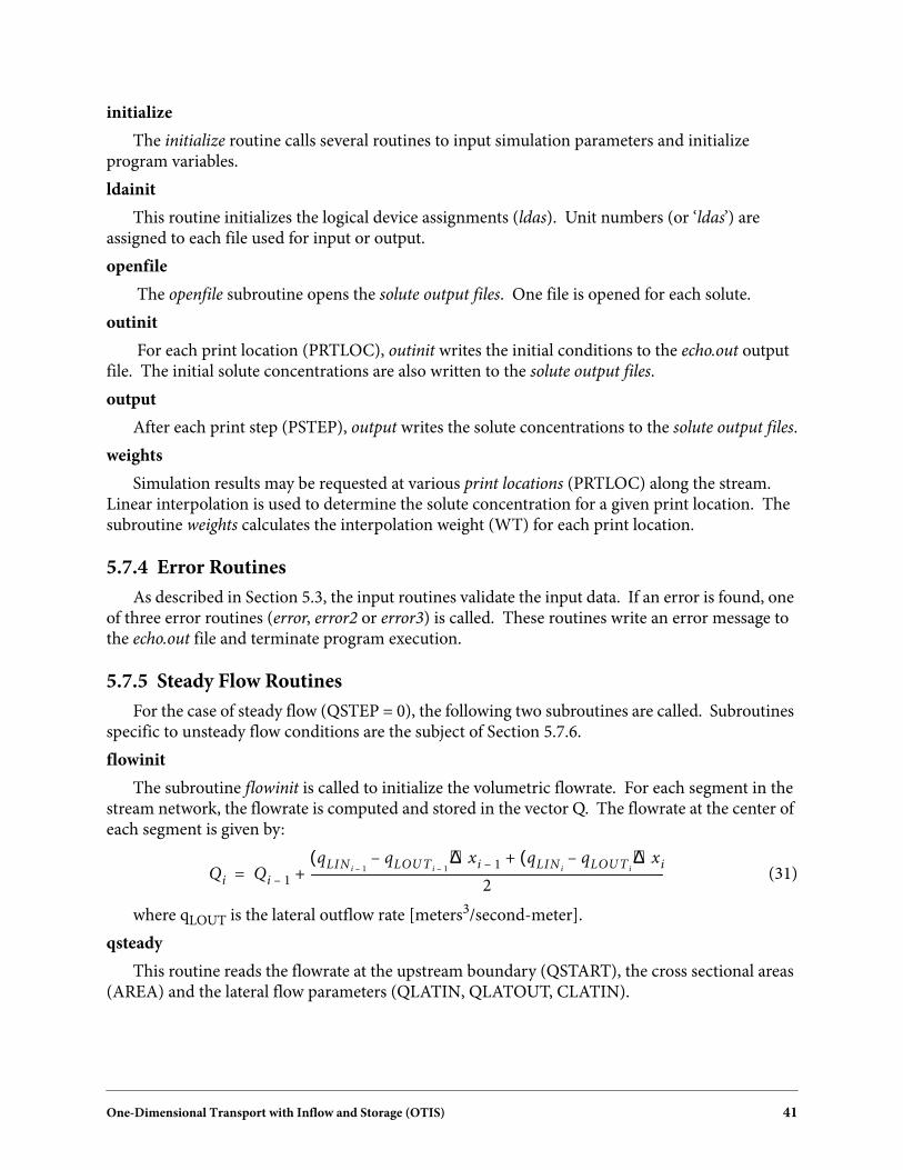
One-Dimensional Transport with Inflow and Storage (OTIS) 41
initialize
The initialize routine calls several routines to input simulation parameters and initializeprogram variables.
ldainit
This routine initializes the logical device assignments (ldas). Unit numbers (or ‘ldas’) areassigned to each file used for input or output.
openfile
The openfile subroutine opens the solute output files. One file is opened for each solute.
outinit
For each print location (PRTLOC), outinit writes the initial conditions to the echo.out outputfile. The initial solute concentrations are also written to the solute output files.
output
After each print step (PSTEP), output writes the solute concentrations to the solute output files.
weights
Simulation results may be requested at various print locations (PRTLOC) along the stream.Linear interpolation is used to determine the solute concentration for a given print location. Thesubroutine weights calculates the interpolation weight (WT) for each print location.
5.7.4 Error Routines
As described in Section 5.3, the input routines validate the input data. If an error is found, oneof three error routines (error, error2 or error3) is called. These routines write an error message tothe echo.out file and terminate program execution.
5.7.5 Steady Flow Routines
For the case of steady flow (QSTEP = 0), the following two subroutines are called. Subroutinesspecific to unsteady flow conditions are the subject of Section 5.7.6.
flowinit
The subroutine flowinit is called to initialize the volumetric flowrate. For each segment in thestream network, the flowrate is computed and stored in the vector Q. The flowrate at the center ofeach segment is given by:
(31)
where qLOUT is the lateral outflow rate [meters3/second-meter].
qsteady
This routine reads the flowrate at the upstream boundary (QSTART), the cross sectional areas(AREA) and the lateral flow parameters (QLATIN, QLATOUT, CLATIN).
Qi Qi 1–
qLIN i 1–qLOU T i 1–
–( )∆xi 1– qLIN iqLOU T i
–( )∆xi+
2----------------------------------------------------------------------------------------------------------------+=

42 One-Dimensional Transport with Inflow and Storage (OTIS)
5.7.6 Unsteady Flow Routines
When solute transport is subject to an unsteady flow regime (QSTEP > 0), the followingsubroutines are used.
readq
The readq subroutine is called each time the flow variables change (i.e. every QSTEP hours).Readq reads the lateral flow parameters, the cross-sectional areas and the flowrates from the flowfile.
qainit
Using the weights provided by qweights, the qainit routine computes a flowrate and area foreach stream segment. Linear interpolation is used to fill the flowrate vector, Q, and the area vector,AREA. The lateral inflow parameters (QLATIN and CLATIN) are also set for each segment.
qunsteady
At the beginning of the simulation, qunsteady reads the flow locations and then calls readq toobtain the initial flow parameters.
qweights
Flow and area values are specified at various flow locations (FLOWLOC) along the stream.Linear interpolation is used to determine the flowrate and cross-sectional area for a given streamsegment. The subroutine qweights calculates the interpolation weight (QWT) for each segment.

One-Dimensional Transport with Inflow and Storage (OTIS) 43
FIG
UR
E 1
4S
ub
rou
tine S
tructu
re
ou
tinit
op
enfile
weigh
ts
ldain
ith
eader
inp
ut
flow
init
qw
eights
qain
it
closef
inp
ut1-4
inp
utq
MA
IN
ou
tpu
t
sstatetim
eloo
p
qu
nstead
yq
steady
readq
distan
ce
seefigu
re16
seefigu
re15
Erro
r Ro
utin
es and
Inclu
de F
iles
error3
error2
error
lda.in
c
fmo
du
les.inc
main
init
main
run
Initialize
prep
roc
prep
roc4
setstop
distan
ce
steady
seefigu
re16
prep
roc1-3
deco
mp

44 One-Dimensional Transport with Inflow and Storage (OTIS)
5.7.7 Dynamic Simulation Routines
The following routines are called when a dynamic simulation is conducted.
conser
For the case of conservative transport, the conser subroutine computes the forcing function{R}. The in-stream and storage zone concentrations are then determined.
decay
When solutes undergo first-order decay, the subroutine decay is called to compute {R}. The in-stream and storage zone concentrations are then determined.
dynamic
This routine controls the dynamic simulation by updating boundary conditions and flow vari-ables at the appropriate times.
partial
The dynamic subroutine is charged with the task of updating the upstream boundary condi-tions and the flow variables at the appropriate times. When these updates occur within the inte-gration interval (i.e. Old Time < Time of Change < New Time), a partial time step is taken. Thesubroutine partial takes a partial time-step and then updates the boundary condition or flow vari-ables, as appropriate.
setstop
As discussed above, the upstream boundary conditions and the flow variables change atspecific times during the simulation. The setstop routine is responsible for setting the variableTSTOP equal to the time at which the next change occurs.
timeloop
The timeloop subroutine is used to control the simulation. After computing the number oftime-steps within each print step, a loop is entered and solute concentrations are computed foreach time-step. Simulation results are printed (via the output subroutine) at the appropriate times.
update
The update subroutine is called whenever the upstream boundary condition or the flow vari-ables change at the beginning of the integration interval. Its task is to update the boundary condi-tions and/or the flow variables.
5.7.8 Pre-processing Routines
Several routines are called to pre-compute parameter groups that are constant with respect totime. This preprocessing significantly reduces the required execution time as the computationsare not repeated for each time-step.
preproc1
Preproc1 computes several quantities that are functions of the segment length, DELTAX.
preproc2
Preproc2 computes two quantities that are functions of the in-stream decay coefficient and thestorage zone exchange coefficient.
One-Dimensional Transport with Inflow and Storage (OTIS) 45
preproc3
Preproc3 computes two quantities that are introduced by the storage zone equation. Becausethese quantities are functions of the time-step, preproc3 must be called whenever the time-stepchanges (e.g. when a partial time-step is taken).
preproc4
The matrix coefficients, E, F and G, are computed by this routine. Given these coefficients, thedecomp routine is called to decompose the coefficient matrix. Because the matrix coefficientsdepend on the flow variables, preproc4 must be called each time the flow variables change.
5.7.9 Routines for the Thomas Algorithm
Tridiagonal matrices such as the one shown in Equation (17) may be solved using the ThomasAlgorithm (see Section 5.4.1). The subroutines to implement the Thomas Algorithm are discussedbelow.
decomp
This routine performs the decomposition phase of the Thomas Algorithm. For the simple caseof conservative transport and steady flow, only one call to decomp is made.
substit
The substitution phase of the Thomas Algorithm is completed by the substit routine.
matrix
The matrix subroutine conducts both phases of the Thomas Algorithm.

46 One-Dimensional Transport with Inflow and Storage (OTIS)
FIG
UR
E 1
5T
ime-V
ariable S
ub
rou
tines
readq
qain
itp
repro
c4setsto
pp
repro
c3p
repro
c4read
ainit
setstop
decay
con
seru
pd
atep
artial
sub
stit
deco
mp
timelo
op
decay
con
sersub
stitd
ecom
p
ou
tpu
td
ynam
ic

One-Dimensional Transport with Inflow and Storage (OTIS) 47
5.7.10 Steady-State Routines
When a steady-state solution is desired, the following routines are used.
sstate
Sstate calls the routines to compute the steady-state concentrations.
ssdiff
The steady-state finite difference routine, ssdiff, computes the matrix coefficients (E, F and G)and the forcing function (R) developed in Appendix D. The matrix subroutine is then called tocompute the steady-state solute concentrations.
sstorage
This routine computes the steady-state concentration in the storage zone.
6.0 MODEL APPLICATION
OTIS has been used to simulate the behavior of conservative and nonconservative solutes in aRocky Mountain stream affected by acid mine drainage. The stream is St. Kevin Gulch, nearLeadville, Colorado, where interdisciplinary studies have addressed physical, chemical, andbiological processes governing the transport and fate of toxic metals in surface waters (Kimball,1991).
FIGURE 16Steady-State Subroutines
ssdiff sstorage
sstate
matrix
steady output

48 One-Dimensional Transport with Inflow and Storage (OTIS)
In the applications shown below, OTIS is used in both dynamic and steady-state modes.These simulations are discussed in greater detail by Kimball et al. (1991). In Section 6.1, wedescribe a dynamic simulation of lithium chloride, an injected tracer. In Section 6.2, two steady-state simulations for iron are presented.
6.1 Application 1: Transient Profiles of a Tracer Salt
OTIS simulated concentration profiles of lithium and chloride during a tracer-dilution experi-ment in St. Kevin Gulch in August 1986. A 4.7 molar solution of lithium chloride was injected intothe stream for 52 hours at an average rate of 27 milliliters per minute. Water samples werecollected at six downstream locations.
Figure 17 shows the control.inp file for the simulation. The control file specifies a single runwith constant parameters read from the file params.inp and flow information read from the fileflow.inp. Simulated lithium and chloride concentrations are written to the files lithium.out andchloride.out, respectively.
The parameter file is shown in Figure 18. For this simulation, stream concentrations areprinted every 0.1 hours. The time step is 0.01 hours, beginning at 13.9 hours and ending at 82.0hours. The upstream boundary of the network is designated 0.0 meters. There is no dispersiveflux at the downstream boundary.
The stream is divided into seven reaches, with reaches one through six ending at the samplinglocations. The last reach extends an additional 100 meters downstream. This reach is included toreduce any error introduced by the downstream boundary approximation (see Section 3.6.2).Reaches vary in length, but each segment within the network is 1.0 meters long. Three reach-specific parameters - the dispersion coefficient, cross-sectional area of the storage zone, and thestream-storage exchange coefficient - are defined. Two solutes, lithium and chloride, are conser-vative throughout the network. Six print locations correspond to the sampling locations. Theupstream boundary concentration is a block-shaped pulse of lithium chloride lasting from 14.0hours until 66.0 hours.
FIGURE 17 Control File for Application 1
1params.inpflow.inplithium.outchloride.out

One-Dimensional Transport with Inflow and Storage (OTIS) 49
The flow file is shown in Figure 19. The zero value in the first line specifies steady-flow condi-tions. Flow at the upstream boundary is 6.12 x 10 -3 cubic meters per second and increases down-stream until the last two reaches, where there is a loss of water from the channel. Stream cross-sectional areas and concentrations of lithium and chloride in lateral inflow waters are specified.
1 2 3 4 5 6 7 8 9101010101010101112131213121312131213121312131415151515151516171717
Application 1: Transient profile of a tracer salt10.100.0113.982.00.00.07 26 26.00 0.02 0.050 3.00E-05458 458.00 0.02 0.050 2.00E-05 42 42.00 0.02 0.250 2.00E-05422 422.00 0.02 0.100 1.50E-05609 609.00 0.02 0.200 5.00E-05247 247.00 0.02 0.200 3.00E-05100 100.00 0.02 0.200 3.00E-0520.00 0.000.00 0.000.00 0.000.00 0.000.00 0.000.00 0.000.00 0.000.00 0.000.00 0.000.00 0.000.00 0.000.00 0.000.00 0.000.00 0.006 26.00 484.00 526.00 948.001557.001804.00312.0 0.005 0.20014.0 2.363 13.36066.0 0.005 0.200
FIGURE 18Parameter File for Application 1

50 One-Dimensional Transport with Inflow and Storage (OTIS)
A post-processor program (see Section 4.6) converted the two solute output files into files witha data format suitable for display by Xgraph. This display for lithium at two sampling locationsreveals a good fit between measured and simulated concentrations (Figure 20). A third output file,echo.out, contains a summary of the simulation parameters. This file is included as Appendix E.
4.120E-06 0.000E-00 0.199 0.005 0.2004.840E-06 0.000E-00 0.152 0.005 0.2000.000E-00 2.030E-05 0.153 0.005 0.2000.000E-00 2.030E-05 0.153 0.005 0.200
3 3 3 3
FIGURE 19Flow File for Application 1
0.00 16.12E-03 20.000E-00 0.000E-00 0.120 0.005 0.2003.780E-06 0.000E-00 0.097 0.036 0.9001.700E-04 0.000E-00 0.138 0.005 0.200
3 3 3
FIGURE 20Dynamic Simulation (Application 1)
Lit
hiu
m C
on
cen
trat
ion
[m
ass/
met
ers3
]
Time [hours]
x measured @ 1804 m
measured @ 525 m
simulated @ 525 m
simulated @ 1804 m

One-Dimensional Transport with Inflow and Storage (OTIS) 51
6.2 Application 2: Steady-State Simulations of Iron Concentration
Two steady-state simulations for iron illustrate the reactive transport of solutes in St. KevinGulch. These simulations use hydraulic parameters calibrated from the simulation of lithium andchloride concentration during the tracer-dilution experiment described in Section 6.1. Iron entersSt. Kevin Gulch with drainage from abandoned mine tailings that flank the stream along a zoneapproximately 363 to 484 meters downstream from the tracer injection site. One additional reachis delineated in this zone to simulate iron loading more accurately. Iron concentration in thedrainage water is characterized by analysis of water samples collected from seeps near the tailings.Lateral inflow rates are calculated based on local dilution of the tracer salt.
The control file shown in Figure 21 specifies two runs with different parameter files but thesame flow file. The two parameter files differ only in record types 12 and 13, which define first-order removal constants. In the file feparams1.inp (Figure 22), these constants are zero throughoutthe network, so that iron is modeled as a conservative substance. In the file feparams2.inp (Figure23), the first-order removal constant varies from 4.0 x 10⁻⁵ to 6.0 x 10⁻⁴ per second. The flow file isshown in Figure 24. A plot of measured and simulated concentrations for the two runs indicatesthat iron is removed as it is transported downstream (Figure 25).
FIGURE 21Control File for Application 2
feflow.inpfe2.out
2feparams1.inpfeflow.inpfe1.outfeparams2.inp

52 One-Dimensional Transport with Inflow and Storage (OTIS)
FIGURE 22Parameter File for Application 2 (Run 1)
1 2 3 4 5 6 7 8 910
Application 2: Steady-state iron with no decay10.000.000.000.000.00.08 26 26.00 0.02 0.050 3.00E-05
101010101010111213121312131213121312131213
1415
15151515151617
10121 121.00 0.02 0.050 2.00E-05 42 42.00 0.02 0.250 2.00E-05422 422.00 0.02 0.100 1.50E-05609 609.00 0.02 0.200 5.00E-05247 247.00 0.02 0.200 3.00E-05100 100.00 0.02 0.200 3.00E-0510.000.000.000.000.000.000.000.000.000.000.000.000.000.00
7 26.00
484.00 526.00 948.001557.001804.0010.00 0.640
337 337.00 0.02 0.050 2.00E-05
1213
0.000.00
15 363.00

One-Dimensional Transport with Inflow and Storage (OTIS) 53
FIGURE 23Parameter File for Application 2 (Run 2)
1 2 3 4 5 6 7 8 910
Application 2: Steady-state iron with decay10.000.000.000.000.00.08 26 26.00 0.02 0.050 3.00E-05
101010101010111213121312131213121312131213
1415
15151515151617
10121 121.00 0.02 0.050 2.00E-05 42 42.00 0.02 0.250 2.00E-05422 422.00 0.02 0.100 1.50E-05609 609.00 0.02 0.200 5.00E-05247 247.00 0.02 0.200 3.00E-05100 100.00 0.02 0.200 3.00E-0510.000.000.000.004.E-54.E-56.E-46.E-49.E-59.E-58.E-58.E-58.E-58.E-5
7 26.00
484.00 526.00 948.001557.001804.0010.00 0.64
337 337.00 0.02 0.050 2.00E-05
1213
8.E-58.E-5
15 363.00

54 One-Dimensional Transport with Inflow and Storage (OTIS)
4.120E-06 0.000E-00 0.199 0.56E+04.840E-06 0.000E-00 0.152 0.56E+00.000E-00 2.030E-05 0.153 0.56E+00.000E-00 2.030E-05 0.153 0.56E+0
3 3 3 3
FIGURE 24Flow File for Application 2
0.00 16.12E-03 20.000E-00 0.000E-00 0.120 0.56E+0
3.780E-06 0.000E-00 0.097 2.11E+21.700E-04 0.000E-00 0.138 0.56E+0
3
3 3
3 3.780E-06 0.000E-00 0.097 0.56E+0
FIGURE 25Steady-State Simulation (Application 2)
Distance [meters x 10-3]
Iro
n C
on
cen
trat
ion
[m
ass/
met
ers3
]
measured concentrations
Run 1 - without decay
Run 2 - with decay

One-Dimensional Transport with Inflow and Storage (OTIS) 55
7.0 CONCLUDING REMARKS
The foregoing sections provide a thorough description of a solute transport model for smallstreams. As presently implemented, the model is capable of simulating the transport of multipleconservative solutes in advective surface water systems. Selected non-conservative substances mayalso be simulated through the specification of first-order decay rates. In addition to providingdynamic and steady-state simulation options, the code allows for the analysis of solute behaviorunder both steady and unsteady flow regimes.
Future work efforts should be directed toward the following tasks:
• Non-conservative solutes are simulated using first-order decay rates. This empiricalapproach does not begin to consider the complex chemical, physical and biological processesthat affect solute transport. In order to increase its utility, the model should be modified toincorporate kinetic and/or equilibrium controlled reactions. Of particular interest is theability to simulate chemical speciation and sorption.
• The model described herein is a stand-alone computer program developed in Fortran-77.As such, the model uses conventional ‘flat files’ for input and output. In order to provide amore flexible modeling environment, an interface-driven version of the code is currentlyunder development (OTIS-MHMS). Parallel development of OTIS and OTIS-MHMSshould continue.
• Section 4.3 presents a model network in which the stream is a linear series of reaches.Future work efforts could include the modifications necessary to simulate solute transport inbranching stream networks.
• Further testing of the unsteady flow option (Section 4.2.3) is needed.

56 One-Dimensional Transport with Inflow and Storage (OTIS)
References
Alley, W.M. and P.E. Smith, Distributed Routing Rainfall-Runoff Model, Version II, Computer Pro-gram Documentation, User’s Manual, U.S. Geological Survey, Water Resources Division, Open-File Report 82-344, 1982.
Arden, B.W. and K.N. Astill, Numerical Algorithms: Origins and Applications, Addison-Wesley,Reading MA, 1970.
Bencala, K.E. and R.A. Walters, Simulation of Solute Transport in a Mountain Pool-and-RiffleStream: A Transient Storage Model, Water Resources Research, 19(3), 718-724, 1983.
Bencala, K.E. and R.A. Walters, Dynamic Solute-Transport Simulation in Dispersive Streamflow,Fortran code obtained from the USGS Prime Computer, August 2, 1990.
Chapra, S.C. and K.H. Reckhow, Engineering Approaches for Lake Management, Volume 2: Mecha-nistic Modeling, Butterworth Publishers, 1983.
Chapra, S.C. and R.P. Canale, Numerical Methods for Engineers, Second Addition, McGraw-Hill,New York, 1988.
Fischer, H.B., E.J. List, R.C.Y. Koh, J. Imberger and N.H. Brooks, Mixing in Inland and Coastal Wa-ters, Academic Press, San Diego, 1979.
Harrison, D., Xgraph Version 11.3.2, University of California, Berkeley, 1989.
Henderson, F.M., Open Channel Flow, Macmillan, New York, 1966.
Jackman, A.P., R.A. Walters and V.C. Kennedy, Transport and Concentration Controls for Chlo-ride, Strontium, Potassium and Lead in Uvas Creek, A Small Cobble-bed Stream in Santa ClaraCounty, California, U.S.A., 2. Mathematical Modeling, Journal of Hydrology, 75:111-141,1984.
Kimball, B.A., Physical, Chemical and Biological Processes in Waters Affected by Acid MineDrainage: From Headwater Streams to Downstream Reservoirs, in U.S. Geological SurveyToxic Substances Hydrology Program, Abstracts of the Technical Meeting Monterey, Califor-nia, March 11-15, 1991, Gail E. Mallard and David A. Aronson, compilers. U.S. GeologicalSurvey Open-File Report 91-88, Page 51, 1991.
Kimball, B.A., R.E. Broshears, K.E. Bencala and D.M. McKnight, Comparison of Rates of Hydro-logic and Chemical Processes in a Stream Affected by Acid Mine Drainage, in U.S. GeologicalSurvey Toxic Substances Hydrology Program, Abstracts of the Technical Meeting Monterey,California, March 11-15, 1991, Gail E. Mallard and David A. Aronson, compilers. U.S. Geo-logical Survey Open-File Report 91-88, Page 71, 1991.
Nordin, C.F. and B.M. Troutman, Longitudinal Dispersion in Rivers: The Persistence of Skewnessin Observed Data, Water Resources Research 16(1), 123-128, 1980.
Thackston, E.L. and P.A. Krenkel, Longitudinal Mixing in Natural Streams, Journal of the SanitaryEngineering Division, ASCE, 93(SA5), 67-90, 1967.

One-Dimensional Transport with Inflow and Storage (OTIS) 57
Thackston, E.L. and K.B. Schnelle, Predicting Effects of Dead Zones on Stream Mixing, Journal ofthe Sanitary Engineering Division, ASCE, 96(SA2), 319-331, 1970.
Thomann, R.V. and J.A. Mueller, Principles of Surface Water Quality Modeling and Control, Harper& Row, New York, 1987.
Valentine, E.M. and I.R. Wood, Longitudinal Dispersion with Dead Zones, Journal of the Hydrau-lics Division, ASCE, 103(HY9), 975-990, 1977.
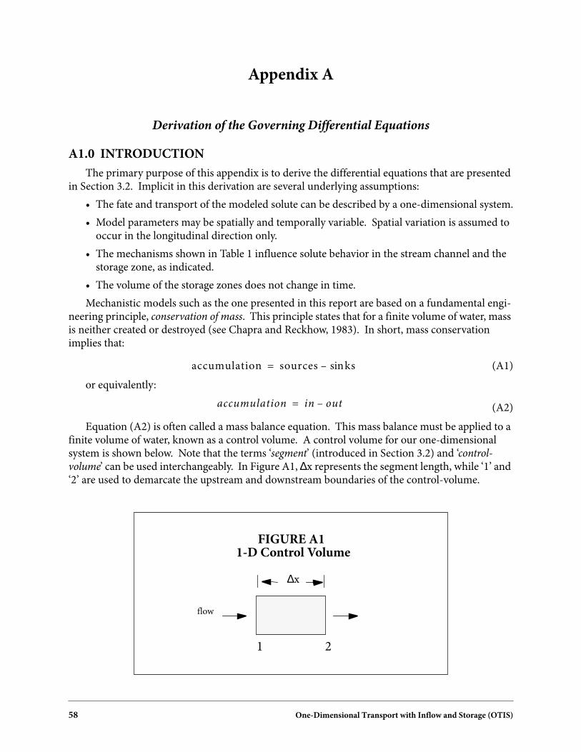
58 One-Dimensional Transport with Inflow and Storage (OTIS)
Appendix A
Derivation of the Governing Differential Equations
A1.0 INTRODUCTION
The primary purpose of this appendix is to derive the differential equations that are presentedin Section 3.2. Implicit in this derivation are several underlying assumptions:
• The fate and transport of the modeled solute can be described by a one-dimensional system.
• Model parameters may be spatially and temporally variable. Spatial variation is assumed tooccur in the longitudinal direction only.
• The mechanisms shown in Table 1 influence solute behavior in the stream channel and thestorage zone, as indicated.
• The volume of the storage zones does not change in time.
Mechanistic models such as the one presented in this report are based on a fundamental engi-neering principle, conservation of mass. This principle states that for a finite volume of water, massis neither created or destroyed (see Chapra and Reckhow, 1983). In short, mass conservationimplies that:
(A1)
or equivalently:
(A2)
Equation (A2) is often called a mass balance equation. This mass balance must be applied to afinite volume of water, known as a control volume. A control volume for our one-dimensionalsystem is shown below. Note that the terms ‘segment’ (introduced in Section 3.2) and ‘control-volume’ can be used interchangeably. In Figure A1, ∆x represents the segment length, while ‘1’ and‘2’ are used to demarcate the upstream and downstream boundaries of the control-volume.
accumulation sources kssin–=
accumulation in out–=
FIGURE A1
∆x
1-D Control Volume
1 2
flow

One-Dimensional Transport with Inflow and Storage (OTIS) 59
The remainder of this appendix is devoted to the formulation of differential equations basedon Equation (A2). To accomplish this task, we first define ‘accumulation’ and then proceed todevelop the ‘in’ and ‘out’ terms for each process given in Table 1. This procedure is carried out forboth the stream channel and the storage zone.
A2.0 MASS BALANCE - STREAM CHANNEL
I. Accumulation
By definition, accumulation is the change in mass with respect to time. For the main streamchannel, accumulation is given by:
(A3)
where
C - in-stream solute concentration [mass/meters3]
V - volume of the main channel segment [meters3]
t - time [seconds]
We can now expand Equation (A3) using the chain rule, yielding:
(A4)
where
∆x - segment length [meters]
A - stream channel cross-sectional area [meters2]
II. Advection
We now begin to develop the ‘in’ and ‘out’ terms for each process. The mass advected into thecontrol volume, i.e. across the upstream boundary, is given by:
(A5)
where Q is the volumetric flowrate [meters3/second].
Next, the mass advected out of the control volume, i.e. across the downstream boundary, isgiven by:
(A6)
Finally, we combine the ‘In’ and ‘Out’ terms, giving:
(A7)
accumulationVC( )∂
t∂---------------=
VC( )∂t∂
--------------- VC∂t∂
------ CV∂t∂
------+ ∆xAt∂
∂C ∆xCt∂
∂A+= =
In QC( )1=
Out QC( )2 QC( )1 x∂∂
QC( )∆x+= =
In Out–x∂
∂QC( )∆x– Q
x∂∂C
Cx∂
∂Q+
∆x–= =

60 One-Dimensional Transport with Inflow and Storage (OTIS)
III. Dispersion
In a similar fashion, we define the dispersive flux across the upstream and downstream bound-aries:
(A8)
(A9)
(A10)
where D is the dispersion coefficient [meters2/second].
IV. Lateral Flows
Here we are interested in mass entering the system via lateral inflow, and mass leaving throughlateral outflow. Note that unlike the previous two mechanisms, the concentrations associated withmass inflows and outflows differ (CL vs. C):
(A11)
(A12)
(A13)
where
CL - solute concentration of the lateral inflow [mass/meters3]
qLIN - lateral inflow rate [meters3/second-meter]
qLOUT - lateral outflow rate [meters3/second-meter]
V. Transient Storage
The final physical mechanism we consider for the stream channel is transient storage. Theinflow and outflow terms are given by:
(A14)
(A15)
(A16)
where
α - storage zone exchange coefficient [/second]
CS - storage zone solute concentration [mass/meters3]
Note that the exchange coefficient, α, is defined as the fraction of the main channel volumethat is exchanged with the storage zone, per unit time.
In ADx∂
∂C
1–=
Out ADx∂
∂C
1 x∂∂
ADx∂
∂C ∆x+–=
In Out–x∂
∂AD
x∂∂C
∆x=
In CLqLIN∆x=
Out CqLOUT∆x=
In Out– CLqLIN CqLOUT–( )∆x=
In αVCS=
Out αVC=
In Out– αV CS C–( ) α∆xA CS C–( )= =

One-Dimensional Transport with Inflow and Storage (OTIS) 61
VI. Decay
In addition to the foregoing physical processes, we also consider the loss of solute mass due tofirst order decay. Since decay represents a one-way loss from the system, our ‘In’ term is zero. Thisresults in:
(A17)
where λ is the in-stream first-order decay rate [/second]. Note that if λ is a negative number,Equation (A17) yields a positive quantity. In this case, the decay term is actually a first-orderproduction mechanism, wherein solute mass is added to the system.
VII. Accumulation = In - Out
Now that the individual processes have been elucidated, the results from I-VI may be used todevelop the mass balance (Equation (A2)). Setting the accumulation term equal to the combined‘In - Out’ terms and dividing by ∆x gives:
(A18)
Although Equation (A18) represents a mass balance for a one-dimensional stream, it may besimplified using the water balance shown below.
VIII. Water Balance
Like the solute mass balance presented above, a water mass balance is based on conservation ofmass. Here again we develop Equation (A2) for a one-dimensional control volume or streamsegment. Using the assumption of incompressible flow, accumulation is given by:
(A19)
where ρ is the density of water [mass/meters3].
The inflow term for the water balance is the sum of the water advected across the upstreaminterface and the water entering via lateral inflow:
(A20)
Similarly, outflow is the sum of the water advected out and that leaving through lateraloutflow:
(A21)
Finally, the water balance is completed by combining Equations (A19) through (A21), anddividing by ρ∆x:
(A22)
In Out– λVC–=
At∂
∂CC
t∂∂A
+ Qx∂
∂CC
x∂∂Q
+ –
x∂∂
ADx∂
∂C CLqLIN CqLOUT–( ) αA CS C–( ) λAC–+ + +=
Accumulationt∂
∂Vρ( ) ρ∆x
t∂∂A
= =
In Q1ρ qLIN∆xρ+=
Out Q2ρ qLOUT∆xρ+ Q1 x∂∂Q∆x+
ρ qLOUT∆xρ+= =
t∂∂A
x∂∂Q
– qLIN qLOUT–( )+=

62 One-Dimensional Transport with Inflow and Storage (OTIS)
IX. Governing Equation - Stream Channel
Substituting Equation (A22) into Equation (A18) and dividing by A yields the governingdifferential equation for the stream channel:
(A23)
This equation is presented in Section 3.2.1 as Equation (1).
A3.0 MASS BALANCE - STORAGE ZONE
As in Section A2.0, a mass balance procedure is used to develop the governing equation. Herethe approach is greatly simplified, as the processes of advection, dispersion and lateral inflow donot affect the storage zone.
I. Accumulation
Accumulation of solute mass in the storage zone is given by:
(A24)
where
VS - volume of the storage zone segment [meters3]
AS - storage zone cross-sectional area [meters2]
Note that the storage zone area, AS, is assumed to be constant in time.
II. Transient Storage
The change in storage zone solute mass is given by:
(A25)
(A26)
(A27)
where α is the fraction of the main channel volume that is exchanged with the storage zone,per unit time.
III. Decay
First-order decay also occurs in the storage zone:
(A28)
where λS is the storage-zone first-order decay coefficient [/second]. Note that the rate of decayin the storage zone is independent from that in the main channel.
t∂∂C Q
A---
x∂∂C
–1
A---
x∂∂
ADx∂
∂C( )
qLIN
A---------- CL C–( ) α CS C–( ) λC–+ + +=
t∂∂
V SCS( ) V S t∂∂CS
CS t∂∂V S
+ ∆xAS t∂∂CS
= =
In αVC=
Out αV CS=
In Out– α∆xA C CS–( )=
In Out– λSV SCS–=
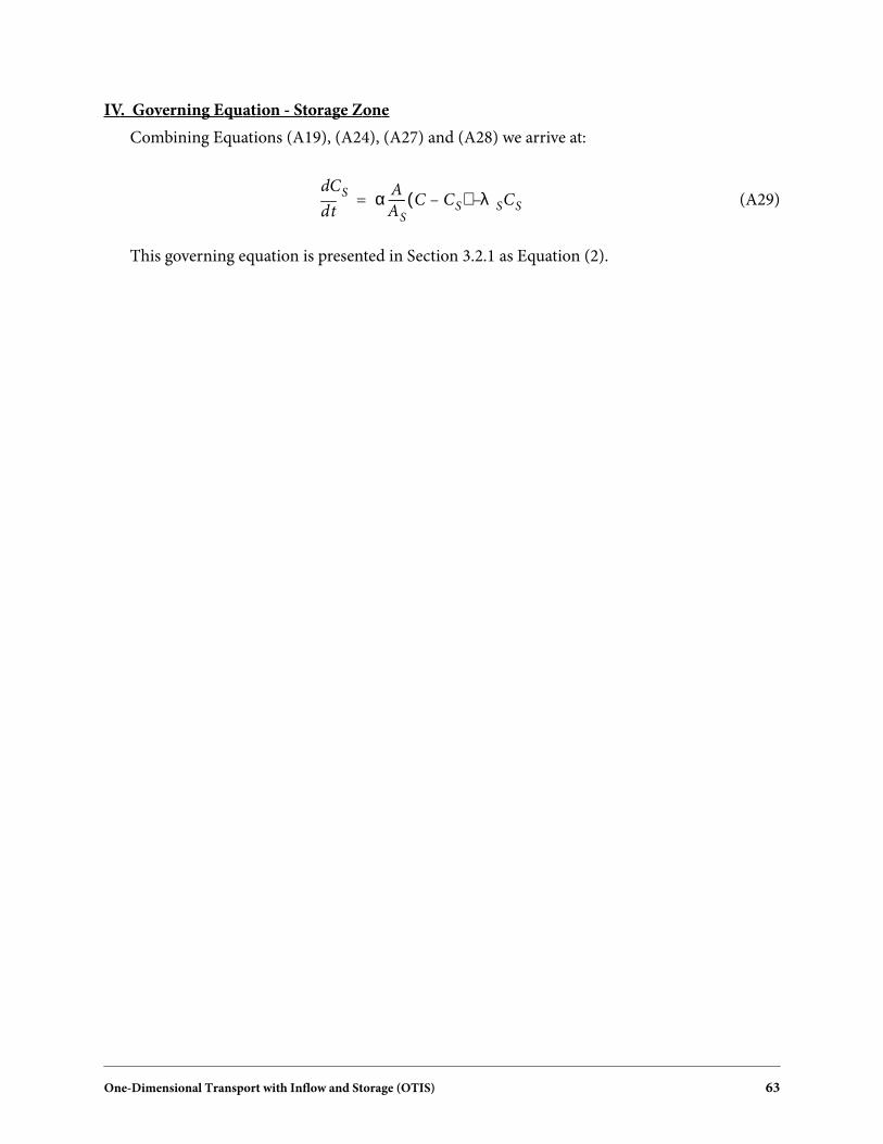
One-Dimensional Transport with Inflow and Storage (OTIS) 63
IV. Governing Equation - Storage Zone
Combining Equations (A19), (A24), (A27) and (A28) we arrive at:
(A29)
This governing equation is presented in Section 3.2.1 as Equation (2).
td
dCS α A
AS
------ C CS–( ) λSCS–=

64 One-Dimensional Transport with Inflow and Storage (OTIS)
Appendix B
Finite Difference Approximations and Boundary Conditions
B1.0 INTRODUCTION
As discussed in Section 3.4, the spatial derivatives in the governing differential equations maybe approximated using finite difference techniques. These techniques are the subject of thisappendix. For a review of finite difference modeling, the reader is referred to Thomann andMueller (1987).
We begin the discussion with a brief overview of the finite difference approximations requiredfor the one-dimensional stream network. This overview is followed by a development of the equa-tions for the individual segments or control-volumes that comprise the system. Two concludingsections discuss a special case of the approximations, boundary conditions.
B2.0 FINITE DIFFERENCE EQUATIONS (FDEs)
Equation (1), the mass balance equation for the stream channel, contains several spatial deriv-atives that may be approximated via finite differences. In general, spatial derivatives and modelparameters need to be defined at both the center of the stream segment and at the segment’s inter-faces. These locations are defined in Figure B1, where an arbitrary quantity, n, is shown. Here wesee that the subscript ‘i’ is used to represent the quantity at the center of the segment. Quantities atthe upstream interface, where segment i-1 adjoins segment i, are indicated using the subscript ‘i-1,i’. In a similar fashion, the downstream interface is marked using the subscript ‘i,i+1’.
I. The Center of the Segment
The first task is to evaluate the spatial derivative, ∂n/∂x, at the center of segment i. Using acentered difference, the spatial derivative of any variable is given by:
(B1)
FIGURE B1Central and Interfacial Quantities
ni, i+1ni-1,i
flow
∆xi-1 ∆xi ∆xi+1
ni-1 ni ni+1
n∂x∂
-----i
ni i 1+, ni 1– i,–
∆xi
---------------------------------=

One-Dimensional Transport with Inflow and Storage (OTIS) 65
Note that Equation (B1) introduces the interfacial quantities, ni-1,i and ni,i+1. Since the massbalance equations were developed for the center of each segment, the interfacial quantities shouldbe defined in terms of ni-1, ni and ni+1. To do this, we compute the interfacial quantities by inter-polating linearly between the centers of the adjacent segments. This results in the following defini-tions:
(B2)
(B3)
II. The Segment Interfaces
We must also define the spatial derivatives at the upstream and downstream interfaces of thesegment. These spatial derivatives are defined as the change in n divided by the distance overwhich the change occurs. For the upstream interface, this gives:
(B4)
The same approach is used to evaluate the spatial derivative at the downstream boundary. Thisyields:
(B5)
B3.0 INTERIOR SEGMENTS - FDEs
Using the foregoing definitions, it is now possible to approximate the spatial derivatives inEquation (1). Note that the first term on the right-hand side of Equation (1) is the ‘Advection’ termwhile the second is the ‘Dispersion’ term. These two quantities are now approximated for the inte-rior segments of the stream network. Boundary segments, i.e. the first and last segments, representspecial cases that are discussed in Sections B4.0 and B5.0
I. Advection
Using definition (B1), the advective term may be approximated as:
(B6)
We now replace the interfacial concentrations (Ci,i+1 and Ci-1,i) with the definitions given byEquations (B2) and (B3). This substitution results in a centered difference approximation for∂C/∂x, given equal segment lengths:
ni 1– i,∆xi
∆xi 1– ∆xi+----------------------------ni 1–
∆xi 1–
∆xi 1– ∆xi+----------------------------ni+=
ni i 1+,∆xi
∆xi 1+ ∆xi+----------------------------ni 1+
∆xi 1+
∆xi 1+ ∆xi+----------------------------ni+=
n∂x∂
-----i 1– i,
2 ni ni 1––( )∆xi ∆xi 1–+----------------------------=
n∂x∂
-----i i 1+,
2 ni 1+ ni–( )∆xi ∆xi 1++----------------------------=
Q
A---
C∂x∂
------–
i
Qi
Ai
-----Ci i 1+, Ci 1– i,–
∆xi
----------------------------------- –≅

66 One-Dimensional Transport with Inflow and Storage (OTIS)
(B7)
II. Dispersion
Here again we use definition (B1) to define the spatial derivative:
(B8)
As the right side of Equation (B8) still contains spatial derivatives, we need the definitionsgiven as Equations (B4) and (B5). Replacing the interfacial derivatives, we arrive at:
(B9)
B4.0 THE FIRST SEGMENT - Upstream Boundary Condition
In the previous section, finite difference approximations for the spatial derivatives were devel-oped. These approximations may be applied directly to all interior segments in the streamnetwork. A problem arises, however, when we are dealing with the first segment, as all quantitiesinvolving the subscript i-1 are undefined. Equations (B7) and (B9) must be modified accordingly.
I. Fixing the Upstream Boundary Condition
To effectively implement the finite difference equations for the first segment, an upstreamboundary condition must be defined. This condition is shown in Figure B2, where the interfacialconcentration at the upstream boundary is set to a user-supplied concentration, Cbc. This quantityis known as the upstream boundary condition.
Qi
Ai∆xi
-------------∆xi
∆xi 1+ ∆xi+----------------------------Ci 1+
∆xi 1+
∆xi 1+ ∆xi+----------------------------Ci
∆xi
∆xi 1– ∆xi+----------------------------Ci 1––
∆xi 1–
∆xi 1– ∆xi+----------------------------Ci–+
–=
1
A---
x∂∂
ADC∂x∂
------
i
1
Ai
-----
ADC∂x∂
------
i i 1+,AD
C∂x∂
------
i 1– i,–
∆xi
--------------------------------------------------------------------≅
1
Ai∆xi
------------- ADi i 1+,2 Ci 1+ Ci–( )∆xi ∆xi 1++( )
-------------------------------- ADi 1– i,2 Ci Ci 1––( )∆xi ∆xi 1–+( )
--------------------------------–≅
FIGURE B2Segment 1 - Upstream B.C.
flow C1
Cbc C1,2

One-Dimensional Transport with Inflow and Storage (OTIS) 67
II. Advection
Given the definition of Cbc, Equation (B6) can be modified for use in the first segment:
(B10)
As with the interior segments, replace the interfacial concentration (C1,2) using Equation (B3):
(B11)
III. Dispersion
Using the equation developed for the interior segments, the dispersive term is given by:
(B12)
The first interfacial derivative (at 1,2) is defined as before using Equation (B5). The secondterm (at 0,1), requires an additional equation:
(B13)
Note that the forward difference approximation shown above must be used in lieu of Equation(B4) to avoid introducing C0, the concentration in the non-existent segment zero. Equations (B5)and (B13) may now be used:
(B14)
B5.0 THE LAST SEGMENT - Downstream Boundary Condition
The finite difference equations developed in Section B3.0 must also be modified to accommo-date the last segment in the stream network. The required modifications to Equations (B7) and(B9) are shown below.
I. Fixing the Downstream Boundary Condition
Application of Equations (B7) and (B9) to the last segment results in the introduction of ansolute concentration, Ci+1. This concentration is undefined as segment i+1 does not exist. Thelast segment, i, and the fictitious segment, i+1, are shown in Figure B3.
Q
A---
x∂∂C
–
1
Q1
A1
------C1 2, Cbc–
∆x1
----------------------- –=
Q1
A1∆x1
---------------∆x1
∆x1 ∆x2+-----------------------C2
∆x2
∆x1 ∆x2+( )----------------------------C1 Cbc–+
–=
1
A---
x∂∂
ADC∂x∂
------
i
1
A1
------
ADC∂x∂
------
1 2,AD
C∂x∂
------
0 1,–
∆x1
----------------------------------------------------------≅
C∂x∂
------0 1,
C1 Cbc–
1
2--∆x1
-------------------=
1
A1∆x1
--------------- AD1 2,2 C2 C1–( )∆x1 ∆x2+------------------------- AD0 1,
2 C1 Cbc–( )∆x1
--------------------------–≅

68 One-Dimensional Transport with Inflow and Storage (OTIS)
To eliminate Ci+1 from the finite difference equations, the dispersive flux at the interfacebetween segments i and i+1 is defined as in Equation (27):
(B15)
where DSBOUND is a user-supplied value for the dispersive flux. Note that if DSBOUND isset equal to zero, Equation (27) is a zero gradient boundary condition (Arden and Astill, 1970).
Using the definition of the interfacial first derivative given by Equation (B5), Equation (27) issolved for Ci+1, yielding:
(B16)
Equation (B16) is now used to eliminate Ci+1 from Equations (B7) and (B9).
II. Advection
Substituting Equation (B16) into (B7) and replacing ∆xi+1 with ∆xi, we arrive at the finitedifference approximation of the advection term:
(B17)
FIGURE B3Downstream Boundary Condition
flow Ci-1 Ci Ci+1
DC∂x∂
------
i i 1+,
DC∂x∂
------
i i 1+,
DSBOUND=
Ci 1+
∆xi ∆xi 1++( )DSBOUND
2Di i 1+,------------------------------------------------------------ Ci+=
Q–
A-------
C∂x∂
------
i
Qi
Ai∆xi
-------------
1
2--∆xiDSBOUND
Di i 1+,--------------------------------------- Ci
∆xi
∆xi 1– ∆xi+( )--------------------------------Ci 1––
∆xi 1–
∆xi 1– ∆xi+( )--------------------------------Ci–+
–=

One-Dimensional Transport with Inflow and Storage (OTIS) 69
III. Dispersion
The finite difference approximation of the dispersion term is now developed by substitutingEquation (B16) into (B9) and replacing ∆xi+1 with ∆xi:
(B18)1
A---
x∂∂
ADC∂x∂
------
i
1
Ai∆xi
------------- Ai i 1+, DSBOUND ADi 1– i,2 Ci Ci 1––( )∆xi ∆xi 1–+( )
--------------------------------–=

70 One-Dimensional Transport with Inflow and Storage (OTIS)
Appendix C
Crank-Nicolson Matrix Coefficients
Numerical Solution of the Dynamic Equations
C1.0 INTRODUCTION
As discussed in Section 3.4, the Crank-Nicolson method is used to solve the dynamic solutetransport equations (Equations (2) and (6)). The Crank-Nicolson solution of the main channelequation (Equation (6)) is the subject of this appendix. A similar discussion for the storage zone(Equation (2)) is given in the main body of this report (Section 3.4.4).
The governing equation for the stream channel is given by:
(C1)
where L[C,Q,A,D,∆x] is the finite difference approximation of the advection and dispersionterms, as given in Appendix B. In order to attain second order accuracy in both time and space,Equation (6) is evaluated at the intermediate time level, j+1/2. To this end, the time derivative isapproximated at the intermediate time level using a centered finite difference:
(C2)
where
∆t - the integration time step [seconds]
j - denotes the value of a parameter or variable at the current time
j+1 - denotes the value of a parameter or variable at the advanced time
Furthermore, the right-hand side at j+1/2 is simply the average of the terms evaluated at timesj and j+1. Combining this average with Equation (C2), Equation (6) becomes:
(C3)
where
(C4)
td
dCL C Q A D ∆x, , , ,[ ]
qLIN
Ai
---------- CL Ci–( ) α CS Ci–( ) λCi–+ +=
td
dC
j1
2--+
Cij 1+ Ci
j–
∆t-----------------------=
Cij 1+ Ci
j–
∆t-----------------------
G C CL CS …, , ,[ ] j 1+ G C CL CS …, , ,[ ] j+
2---------------------------------------------------------------------------------------------=
G C CL CS Q A D qLIN ∆x α λ, , , , , , , , ,[ ] L C Q A D ∆x, , , ,[ ]qLIN
Ai
---------- CL Ci–( ) α CS Ci–( ) λCi–+ +=

One-Dimensional Transport with Inflow and Storage (OTIS) 71
Because Equation (9) is dependent on the solute concentrations in the neighboring segmentsat the advanced time level (Ci-1, Ci+1 at time j+1), it is not possible to explicitly solve for Ci
j+1. Inthe sections that follow, Equation (9) is rearranged so that all of the known quantities (i.e. those attime j) appear on the right-hand side and all of the unknown quantities (i.e. those at time j+1)appear on the left. This rearrangement yields:
(C5)
where E, F and G are matrix coefficients and R is a forcing function.
We now proceed to develop the matrix coefficients and the forcing function by examining eachterm in Equation (9). In general, unknown quantities in each term contribute to the matrix coeffi-cients while known quantities make up the forcing function. After going through each term, indi-vidual contributions are summed (see Section C4.0) to obtain E, F, G and R. This analysis assumesthat Q, CL, qLIN, A, λ and α are constant in time. This assumption may introduce some error forsimulations of solute transport under unsteady flow conditions.
C2.0 LEFT-HAND SIDE OF EQUATION C3 - TIME DERIVATIVE
As noted above, Equation (9) must be rearranged to develop the coefficients in Equation (12).We begin this process by considering the left side of Equation (9), the time derivative. Leaving theunknown concentration, Ci
j+1, on the left side and moving the known concentration to the rightside, the contributions are given by:
(C6)
(C7)
C3.0 RIGHT-HAND SIDE OF EQUATION C3
The right side of Equation (9) must also be rearranged such that the unknown quantitiesappear on the left side of Equation (12) and the known quantities appear on the right. As shown inEquation (C4), G[C,CL,CS,...] is made up of several terms. Each term in G[] is examined below.
C3.1 Advection
In Equation (C4), the operator L[C,Q,A,D,∆x] represents the finite difference approximation ofthe spatial derivatives describing advection and dispersion. The contribution of the advectionterm is the subject of this section, while the dispersion term is discussed subsequently.
Using the finite difference equations for the advection term (Equations (B7), (B11), and(B17)), we develop the contributions to the matrix coefficients shown below. Note that due to thepresence of boundary conditions, the contributions depend on the type of segment for whichEquation (12) is developed.
EiCi 1–j 1+ F iCi
j 1+ GiCi 1+j 1++ + Ri=
Fdt1
∆t-----=
Rdt1
∆t-----Ci
j=

72 One-Dimensional Transport with Inflow and Storage (OTIS)
Interior Segments
Consulting Equation (B7), we see that:
(C8)
(C9)
(C10)
(C11)
where E, F and G are given by Equations (C8) through (C10).
First Segment
Using Equation (B11):
(C12)
(C13)
(C14)
Last Segment
Evaluating Equation (B17) at j+1/2 yields:
(C15)
(C16)
(C17)
Eadv
Qi
2Ai ∆xi 1– ∆xi+( )-----------------------------------------–=
Fadv
Qi
2Ai∆xi
----------------∆xi 1+
∆xi 1+ ∆xi+----------------------------
∆xi 1–
∆xi 1– ∆xi+----------------------------–
=
Gadv
Qi
2Ai ∆xi 1+ ∆xi+( )-----------------------------------------=
Radv EadvC ji 1–– FadvCi
j– GadvCi 1+j–=
Fadv
Q1∆x2
2A1∆x1 ∆x1 ∆x2+( )----------------------------------------------=
Gadv
Q1
2A1 ∆x1 ∆x2+( )-------------------------------------=
Radv FadvC1j– GadvC2
j–Q1
A1∆x1
---------------Cbc+=
Eadv
Qi
2Ai ∆xi 1– ∆xi+( )-----------------------------------------–=
Fadv
Qi
2Ai∆xi
---------------- 1∆xi 1–
∆xi 1– ∆xi+----------------------------–
=
Radv EadvC ji 1–– FadvCi
j–Qi
2Ai
--------DSBOUND
Di i 1+,---------------------------–=
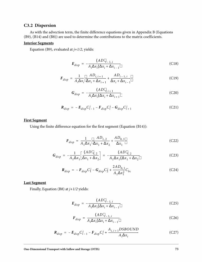
One-Dimensional Transport with Inflow and Storage (OTIS) 73
C3.2 Dispersion
As with the advection term, the finite difference equations given in Appendix B (Equations(B9), (B14) and (B8)) are used to determine the contributions to the matrix coefficients.
Interior Segments
Equation (B9), evaluated at j+1/2, yields:
(C18)
(C19)
(C20)
(C21)
First Segment
Using the finite difference equation for the first segment (Equation (B14)):
(C22)
(C23)
(C24)
Last Segment
Finally, Equation (B8) at j+1/2 yields:
(C25)
(C26)
(C27)
Edisp
AD( )i 1– i,Ai∆xi ∆xi ∆xi 1–+( )----------------------------------------------–=
Fdisp1
Ai∆xi
-------------ADi i, 1+
∆xi ∆xi 1++----------------------------
ADi 1– i,∆xi ∆xi 1–+----------------------------+
=
Gdisp
AD( )i i 1+,Ai∆xi ∆xi ∆xi 1++( )----------------------------------------------–=
Rdisp EdispCi 1–j– FdispCi
j– GdispCi 1+j–=
Fdisp1
A1∆x1
---------------AD1 2,
∆x1 ∆x2+-----------------------
AD0 1,∆x1
--------------+ =
Gdisp1
A1∆x1
---------------AD( )1 2,
∆x1 ∆x2+-----------------------–
AD( )1 2,A1∆x1 ∆x1 ∆x2+( )-------------------------------------------–= =
Rdisp FdispC1j– GdispC2
j–2AD0 1,
A1∆x12
-----------------Cbc+=
Edisp
AD( )i 1– i,Ai∆xi ∆xi ∆xi 1–+( )----------------------------------------------–=
Fdisp
AD( )i 1– i,Ai∆xi ∆xi ∆xi 1–+( )----------------------------------------------=
Rdisp EdispCi 1–j– FdispCi
j–Ai i 1+, DSBOUND
Ai∆xi
-------------------------------------------+=

74 One-Dimensional Transport with Inflow and Storage (OTIS)
C3.3 Lateral Inflow
The third term in G[], lateral inflow, is also evaluated at j+1/2:
(C28)
Assuming qLIN, CL and Ai to be time invariant, Equation (C28) becomes:
(C29)
The contributions are thus:
(C30)
(C31)
C3.4 Transient Storage
The transient storage term is now evaluated at j+1/2:
(C32)
To decouple the governing transport equations (see Section 3.4.5), Equation (19) is used toeliminate CS
j+1. Equation (C32) thus becomes:
(C33)
The contributions to the matrix coefficients are given by:
(C34)
(C35)
qLIN
A---------- CL C–( )
j1
2--+
qLIN
A---------- CL Ci–( )
j qLIN
A---------- CL Ci–( )
j 1+
+
2-------------------------------------------------------------------------------------------=
qLIN
2Ai
---------- 2CL Cij– Ci
j 1+–( )=
F lat
qLIN
2Ai
----------=
Rlat
qLIN
Ai
----------CL
qLIN
2Ai
----------Cij–=
α Cs Ci–( )j
1
2--+ α Cs Ci–( ) j α Cs Ci–( ) j 1++
2-----------------------------------------------------------------
α2--- C j
s Cij– CS
j 1+ Cij 1+–+( )= =
α2--- CS
j Cij– Ci
j 1+–2 γ– ∆tλs–
2 γ ∆tλs+ +----------------------------Cs
j γ2 γ ∆tλs+ +----------------------------Ci
j γ2 γ ∆tλs+ +----------------------------Ci
j 1++ + + =
F storα2--- 1
γ2 γ ∆tλs+ +----------------------------–
=
Rstor F storCij–
α2--- 1
2 γ– ∆tλs–
2 γ ∆tλs+ +----------------------------+
Csj+=

One-Dimensional Transport with Inflow and Storage (OTIS) 75
C3.5 First-Order Decay
The final term in G[] represents first-order decay or production. This term is evaluated atj+1/2:
(C36)
The contributions are given by:
(C37)
(C38)
C4.0 MATRIX COEFFICIENTS
The matrix coefficients (E, F, G) and the forcing function (R) from Equation (12) may now bedeveloped by summing the contributions given in Sections C2.0 and C3.0, and multiplying by ∆t:
(C39)
(C40)
(C41)
(C42)
λC–( )j
1
2--+ λC( ) j– λC( ) j 1+–
2-------------------------------------------
λ2--- Ci
j Cij 1++( )–= =
Fdecayλ2---=
Rdecay FdecayCij–=
Ei ∆t Eadv Edisp+( )=
F i ∆t Fdt Fadv Fdisp F lat F stor Fdecay+ + + + +( )=
Gi ∆t Gadv Gdisp+( )=
Ri ∆t Rdt Radv Rdisp Rlat Rstor Rdecay+ + + + +( )=

76 One-Dimensional Transport with Inflow and Storage (OTIS)
Appendix D
Steady State Matrix Coefficients
The purpose of this appendix is to develop the matrix coefficients (E, F, G) and the forcingfunction (R) from Equation (26). In the text that follows, the contributions to E, F, G and R aregiven on a term-by-term basis. The final values are determined by summing the individual contri-butions.
D1.0 ADVECTION
Equations (B7), (B11), and (B17) are used to approximate the spatial derivative describingadvective transport. These equations contribute to the matrix coefficients as detailed below. Dueto boundary conditions, the contributions depend on the type of segment for which Equation (26)is developed.
Interior Segments
(D1)
(D2)
(D3)
First Segment
(D4)
(D5)
(D6)
Eadv
Qi
Ai
-----1
∆xi 1– ∆xi+----------------------------
–=
Fadv
Qi
Ai∆xi
-------------∆xi 1+
∆xi ∆xi 1++----------------------------
∆xi 1–
∆xi ∆xi 1–+----------------------------–
=
Gadv
Qi
Ai
-----1
∆xi ∆xi 1++----------------------------
=
Fadv
Q1
A1∆x1
---------------∆x2
∆x1 ∆x2+-----------------------
=
Gadv
Q1
A1
------1
∆x1 ∆x2+-----------------------
=
Radv
Q1
A1
------Cbc
∆x1
--------=

One-Dimensional Transport with Inflow and Storage (OTIS) 77
Last Segment
(D7)
(D8)
(D9)
D2.0 DISPERSION
As with the advection term, the finite difference equations given in Appendix B (Equations(B9), (B14) and (B8)) are used to determine the contributions to the matrix coefficients.
Interior Segments
(D10)
(D11)
(D12)
First Segment
(D13)
(D14)
(D15)
Last Segment
(D16)
Eadv
Qi
Ai
-----1
∆xi ∆xi 1–+----------------------------
–=
Fadv
Qi
Ai∆xi
------------- 1∆xi 1–
∆xi ∆xi 1–+----------------------------–
=
Radv
Qi
Ai
-----DSBOUND
2Di i 1+,---------------------------–=
Edisp
2 AD( )i 1– i,Ai∆xi ∆xi ∆xi 1–+( )----------------------------------------------–=
Fdisp2
Ai∆xi
-------------ADi i, 1+
∆xi ∆xi 1++----------------------------
ADi 1– i,∆xi ∆xi 1–+----------------------------+=
Gdisp
2ADi i 1+,Ai∆xi ∆xi ∆xi 1++( )----------------------------------------------–=
Fdisp2
A1∆x1
---------------AD1 2,
∆x1 ∆x2+-----------------------
AD0 1,∆x1
--------------+ =
Gdisp
2AD1 2,A1∆x1 ∆x1 ∆x2+( )-------------------------------------------–=
Rdisp1
A1
------2AD0 1, Cbc
∆x12
-------------------------=
Edisp
2ADi 1– i,Ai∆xi ∆xi ∆xi 1–+( )----------------------------------------------–=

78 One-Dimensional Transport with Inflow and Storage (OTIS)
(D17)
(D18)
D3.0 LATERAL INFLOW
(D19)
(D20)
D4.0 TRANSIENT STORAGE
(D21)
D5.0 DECAY
(D22)
D6.0 MATRIX COEFFICIENTS
The matrix coefficients (E, F, G) and the forcing function (R) from Equation (26) may now bedeveloped by summing the contributions given in Sections D1.0 through D5.0:
(D23)
(D24)
(D25)
(D26)
Fdisp
2ADi 1– i,Ai∆xi ∆xi ∆xi 1–+( )----------------------------------------------=
Rdisp
Ai i 1+, DSBOUND
Ai∆xi
-------------------------------------------=
F lat
qLIN
Ai
----------=
Rlat
qLIN
Ai
----------CL=
F stor
αAsλs
αA Asλs+------------------------=
Fdecay λ=
Ei Eadv Edisp+=
F i Fadv Fdisp F lat F stor Fdecay+ + + +=
Gi Gadv Gdisp+=
Ri Radv Rdisp Rlat+ +=
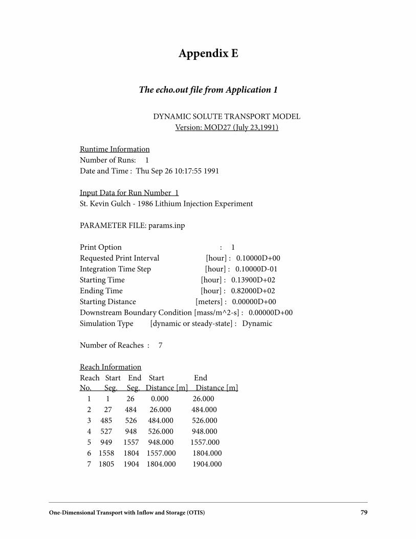
One-Dimensional Transport with Inflow and Storage (OTIS) 79
Appendix E
The echo.out file from Application 1
DYNAMIC SOLUTE TRANSPORT MODEL
Version: MOD27 (July 23,1991)
Runtime Information
Number of Runs: 1
Date and Time : Thu Sep 26 10:17:55 1991
Input Data for Run Number 1
St. Kevin Gulch - 1986 Lithium Injection Experiment
PARAMETER FILE: params.inp
Print Option : 1
Requested Print Interval [hour] : 0.10000D+00
Integration Time Step [hour] : 0.10000D-01
Starting Time [hour] : 0.13900D+02
Ending Time [hour] : 0.82000D+02
Starting Distance [meters] : 0.00000D+00
Downstream Boundary Condition [mass/m^2-s] : 0.00000D+00
Simulation Type [dynamic or steady-state] : Dynamic
Number of Reaches : 7
Reach Information
Reach Start End Start EndNo. Seg. Seg. Distance [m] Distance [m]
1 1 26 0.000 26.000
2 27 484 26.000 484.000
3 485 526 484.000 526.000
4 527 948 526.000 948.000
5 949 1557 948.000 1557.000
6 1558 1804 1557.000 1804.000
7 1805 1904 1804.000 1904.000

80 One-Dimensional Transport with Inflow and Storage (OTIS)
Number of Spatial Segments : 1904
Reach Parameters
Reach No. Reach Segment Dispersion
No. Segs. Length [m] Length [m] Coeff.[m^2/s]
1 26 26.000 1.000 0.20000D-01
2 458 458.000 1.000 0.20000D-01
3 42 42.000 1.000 0.20000D-01
4 422 422.000 1.000 0.20000D-01
5 609 609.000 1.000 0.20000D-01
6 247 247.000 1.000 0.20000D-01
7 100 100.000 1.000 0.20000D-01
Storage Parameters
Storage Storage
Reach Zone Area Rate
No. [m^2] [/sec]
1 0.50000D-01 0.30000D-04
2 0.50000D-01 0.20000D-04
3 0.25000D+00 0.20000D-04
4 0.10000D+00 0.15000D-04
5 0.20000D+00 0.50000D-04
6 0.20000D+00 0.30000D-04
7 0.20000D+00 0.30000D-04
Number of Solutes: 2
Chemistry : Conservative
Decay Coefficients, Solute # 1
Coefficient
Reach Channel Storage
No. [/second] [/second]
1 0.000D+00 0.000D+00
2 0.000D+00 0.000D+00
3 0.000D+00 0.000D+00
4 0.000D+00 0.000D+00
5 0.000D+00 0.000D+00
6 0.000D+00 0.000D+00
7 0.000D+00 0.000D+00

One-Dimensional Transport with Inflow and Storage (OTIS) 81
Decay Coefficients, Solute # 2
Coefficient
Reach Channel Storage
No. [/second] [/second]
1 0.000D+00 0.000D+00
2 0.000D+00 0.000D+00
3 0.000D+00 0.000D+00
4 0.000D+00 0.000D+00
5 0.000D+00 0.000D+00
6 0.000D+00 0.000D+00
7 0.000D+00 0.000D+00
Number of Print Locations : 6
Printing Information
Location [m]
26.000
483.000
526.000
948.000
1557.000
1804.000
Number of Upstream Boundary Conditions: 3
Upstream Boundary Conditions, Solute # 1
Begin Concentration
Time [hour] [mass/m^3]
0.1200D+02 0.0000D+00
0.1400D+02 0.2363D+01
0.6600D+02 0.0000D+00
Upstream Boundary Conditions, Solute # 2
Begin Concentration
Time [hour] [mass/m^3]
0.1200D+02 0.0000D+00
0.1400D+02 0.1336D+02
0.6600D+02 0.0000D+00

82 One-Dimensional Transport with Inflow and Storage (OTIS)
Flow and Area Data
FLOW FILE: flow.inp
Flow Option : Steady
Flow interval [hour] : 0.00000D+00
Initial Flow and Area Values
Flowrate at Upstream Boundary [m^3/sec] : 0.61200D-02
Lateral Lateral X-sect.
Reach Inflow Outflow Area
No. [m^3/s-m] [m^3/s-m] [m^2]
1 0.00000D+00 0.00000D+00 0.12000D+00
2 0.37800D-05 0.00000D+00 0.97000D-01
3 0.17000D-03 0.00000D+00 0.13800D+00
4 0.41200D-05 0.00000D+00 0.19900D+00
5 0.48400D-05 0.00000D+00 0.15200D+00
6 0.00000D+00 0.20300D-04 0.15300D+00
7 0.00000D+00 0.20300D-04 0.15300D+00
Initial Lateral Inflow Concentrations, Solute # 1
Inflow
Reach Concent.
No. [mass/m^3]
1 0.50000D-02
2 0.36000D-01
3 0.50000D-02
4 0.50000D-02
5 0.50000D-02
6 0.50000D-02
7 0.50000D-02

One-Dimensional Transport with Inflow and Storage (OTIS) 83
Initial Lateral Inflow Concentrations, Solute # 2
Inflow
Reach Concent.
No. [mass/m^3]
1 0.20000D+00
2 0.90000D+00
3 0.20000D+00
4 0.20000D+00
5 0.20000D+00
6 0.20000D+00
7 0.20000D+00
Output Files for Solutes
Solute # File Name
1 lithium.out
2 chloride.out
Initial Conditions at the Print Locations
Location Prev. Inter. Flow
[m] Seg. Weight [m^3/sec]
26.00 26 0.500000D+00 0.612094D-02
483.00 483 0.500000D+00 0.784746D-02
526.00 526 0.500000D+00 0.149498D-01
948.00 948 0.500000D+00 0.167301D-01
1557.00 1557 0.500000D+00 0.196712D-01
1804.00 1804 0.500000D+00 0.146633D-01
Initial Conditions, Solute # 1
Concentration
Location Channel Storage
[m] [mass/m^3] [mass/m^3]
26.00 0.000D+00 0.000D+00
483.00 0.000D+00 0.000D+00
526.00 0.000D+00 0.000D+00
948.00 0.000D+00 0.000D+00
1557.00 0.000D+00 0.000D+00
1804.00 0.000D+00 0.000D+00

84 One-Dimensional Transport with Inflow and Storage (OTIS)
Initial Conditions, Solute # 2
Concentration
Location Channel Storage
[m] [mass/m^3] [mass/m^3]
26.00 0.000D+00 0.000D+00
483.00 0.000D+00 0.000D+00
526.00 0.000D+00 0.000D+00
948.00 0.000D+00 0.000D+00
1557.00 0.000D+00 0.000D+00
1804.00 0.000D+00 0.000D+00

One-Dimensional Transport with Inflow and Storage (OTIS) 85
Appendix F
Program Listing
For a copy of the OTIS solute transport code, contact:
Robert L. RunkelCU-CADSWES2945 Center Green CourtSuite BBoulder, Colorado 80301
Robert E. BroshearsU.S. Geological SurveyWater Resources DivisionMail Stop 415Denver Federal CenterLakewood, Colorado 80225