One-dimensional energy balance model

Meridional heat transport andtemperature distribution in the

atmosphere

Recommended reading:Energy balance models

• McGuffie, Kendal and Henderson-Sellers, Ann (2005): A climate modelling primer. 3rd edition. Chichester: Wiley– Chapter 3 Energy Balance Models (pp. 81-116), e.g.

Section 3.2. The Structure of Energy Balance Models (pp. 82-86)

• Walker, J. C. G. (1991): Numerical Adventures with Geochemical Cycles. New York: Oxford University– Chapter 7, Climate: A chain of Identical Reservoirs

Recommended reading:Energy balance models

• Hartmann, Dennis L. (1994): Global Physical Climatology. San Diego: Academic Press– Section 9.4 (p. 236-238)

Recommended reading:Energy balance models

• In German: Stocker, Thomas (2008), Einführung in die Klimamodellierung (lecture notes, 146 pp), http://www.climate.unibe.ch/~stocker/papers/skript08EKM.pdf.

– Section 4.3 (p. 69-70) and Problem 9 (p. 142)

• In German: von Storch, Hans, Stefan Güss, Martin Heimann (1999): Das Klimasystem und seine Modellierung: eine Einführung. Berlin, Heidelberg: Springer-Verlag– Kapitel 4 “Konzptionelle Modelle”, Abschnitt 4.2 “Ein

exemplarisches Energibilanzmodell”

The Earth’s annual and global-mean energy budget

UW Atmospheric Sciences

Insolation (W m-2) at the top of the atmosphere as a function of latitude. Averaged over entire year and at the solstices [Fig. 2.7 from Hartmann (1994)]

Balance between average net shortwave and longwave radiation from 90°N to 90°S [Figure 7j-1 from Pidwirny (2005), http://www.physicalgeography.net/]

 

Meridional energy (heat) flow

Trenberth and Caron 2001

Total transport

Atmospherictransport

Ocean transport

Observed meridonal energy flow in the atmosphere and ocean

outao

F

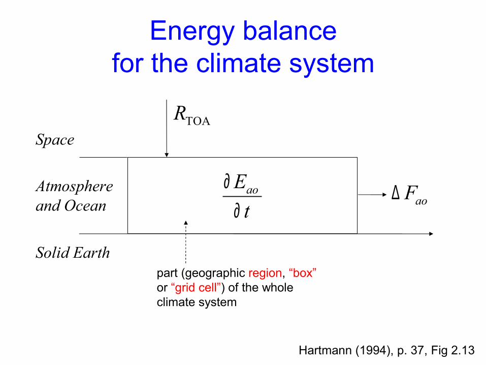
Energy balancefor the climate system

Hartmann (1994), p. 37, Fig 2.13

aoEt

∂∂

Space

Atmosphere and Ocean

Solid Earthpart (geographic region, “box” or “grid cell”) of the whole climate system

SUNTOAR

inao

F change of energy content aoF∆

Energy balancefor the climate system

Hartmann (1994), p. 37, Fig 2.13

aoEt

∂∂

TOARSpace

Atmosphere and Ocean

Solid Earthpart (geographic region, “box” or “grid cell”) of the whole climate system

aoF∆

Energy balancefor the climate system

TOAR net incoming radiation at the top of the atmosphere

aoF∆ divergence of horizontal flux in atmosphere and ocean

time rate of change of energy content of climate system (Eao is proportional to temperature)

aoEt

∂∂

TOA aoaoE R Ft

∂ = − ∆∂

(McGuffie and Henderson-Sellers, 2005)

A 1-d energy balance model (EBM)

resolves latitude-dependence of the energy budget

• Assumptions: – Everything about climate can be characterized

by surface temperature.

– The only independent variable is latitude.

– Energy transport can be approximated by a diffusive process

Hartmann (1994), p. 237

Energy content of an atmosphere-ocean column of unit horizontal area

ao ao s .E C T≈

effective heat capacity (J m-2K-1) of the atmosphere-ocean system

energy content of an atmosphere-ocean column of unit horizontal area extending from the bottom of the ocean mixed layer to the top of atmosphere (TOA)

effective or mean temperature (K) of the atmosphere-ocean system, taken as surface temperature

aoE

aoC

sT

Surface temperature

Simplest description: write as product

• Choose a value for the effective heat capacity that corresponds to the ocean mixed layer– This is the upper 50 to 70 m of the ocean that

is in direct contact with the atmosphere through the ocean surface.

aoC

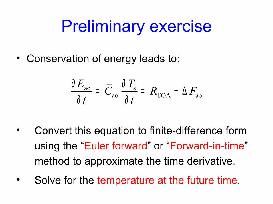
Preliminary exercise

• Conservation of energy leads to:

ao sao TOA ao

E TC R Ft t

∂ ∂= = − ∆∂ ∂

• Convert this equation to finite-difference form using the “Euler forward” or “Forward-in-time” method to approximate the time derivative.

• Solve for the temperature at the future time.

The net incoming radiation at the top of the atmosphere can be written as follows:

TOA ABSR Q F ↑∞= −

ABSQ absorbed solar radiation

F ↑∞ outgoing longwave radiation = ε σ T4

Where:

Notes on the energy balance

Cf. Hartmann, p. 237.

Emissivity = 0.6 („Greenhouse Effect“)

How much of the incoming solar radiation is actually absorbed is determined by the reflectivity or planetary albedo, αp:

QABS = Q (1-αp)

incoming solar (shortwave) radiation

Dependence of albedo on latitude

Highly simplified distribution after Stocker (2008)

Cf. Hartmann, p. 237.

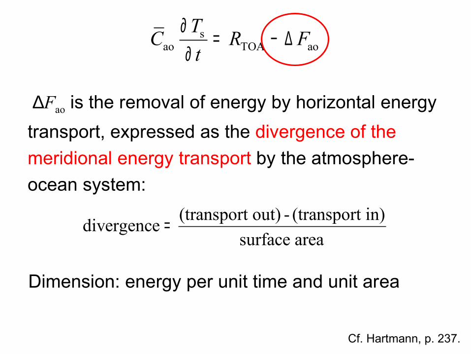
∆Fao is the removal of energy by horizontal energy transport, expressed as the divergence of the meridional energy transport by the atmosphere-ocean system:

(transport out) - (transport in)divergencesurface area

=

Dimension: energy per unit time and unit area

sao TOA ao

TC R Ft

∂ = − ∆∂

Divergence The “spreading out” of a flow or the flux of a quantity away from a point in more than one direction. Convergence is the opposite.

In our case, we refer to the divergence of energy or heat.

From the glossary by McGuffie and Henderson-Sellers (1997).

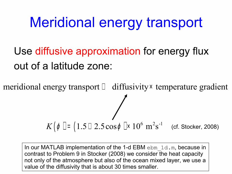
Meridional energy transport

Use diffusive approximation for energy flux out of a latitude zone:

meridional energy transport diffusivity temperature gradient∝ ×

( ) ( ) 6 2 -11.5 2.5cos 10 m sK ϕ ϕ= + × (cf. Stocker, 2008)

In our MATLAB implementation of the 1-d EBM ebm_1d.m, because in contrast to Problem 9 in Stocker (2008) we consider the heat capacity not only of the atmosphere but also of the ocean mixed layer, we use a value of the diffusivity that is about 30 times smaller.

Staggered grids

• Diffusivity and temperature gradient are best defined at the interface between two adjacent temperature grid cells.

• It is convenient to define two grids: one grid for all temperature-related variables (“T grid”), the other grid for all meridional energy transport-related variables (“U grid”)

(More generally, all “tracer”-related variables would be defined at the T grid cell centers, and all “velocity”-related variables would be defined at the U grid cell centers.)

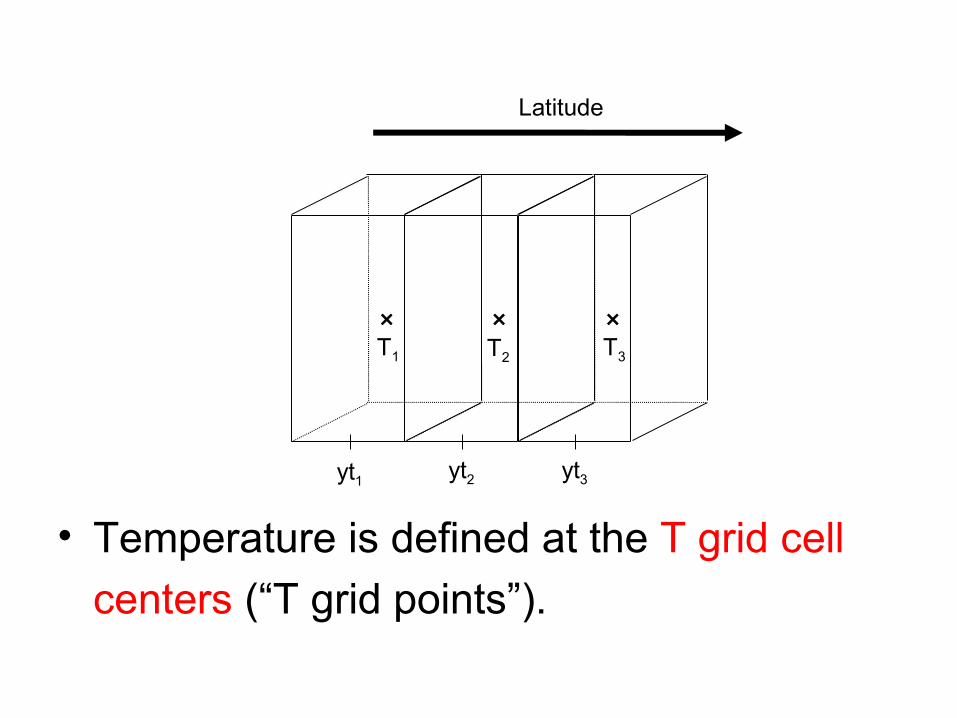
yt1 yt2 yt3

× × ×T1 T2 T3

• Temperature is defined at the T grid cell centers (“T grid points”).

Latitude

yt1 yt2yu1 yu2 yt3 yu3

× × ×× × ×U1 U2 U3

T1 T2 T3

• Diffusivity and temperature gradient are defined at the interfaces of adjacent T grid cells (“U grid points”).

Validity of diffusive approximation

Diffusive approximation to meridional transport is valid for time scales ≥ 6 months and length scales ≥ 1500 km (Lorenz 1979)

• The one-dimensional energy balance model is available from the geo server.– Download ebm_1d.zip from http://www.geo.uni-bremen.de/~apau/ecolmas_modeling2 to your computer and extract the archive (e.g. to “My Documents”)

• Start MATLAB and set current directory to the folder with the model

How to get the model

Exercise 1a

• Run the one-dimensional energy balance model ebm_1d

• Import model output and observed temperature into MATLAB import_data.m

• Plot simulated vs. observed temperature distribution plot_data.m

Import model output

• To import the ebm_1d output files, use the MATLAB textread function, specifying the headerlines parameter, e.g.:

[yt solin apln netswpln netlwpln div_eddy tatm] = ...textread('energy_balance_1d.dat',...'%f %f %f %f %f %f %f','headerlines',10)See the M-file script: import_data.m

Import NCEP data

• To import the observed temperature distribution, also use the MATLAB textread function:

[yncep tncep] = textread('NCEP_air_zonal_ann.dat‘,...'%f %f','headerlines',5)

See the M-file script: plot_data.m

Exercise 1b

• Plot the incoming shortwave and outgoing longwave radiation. Discuss if the pattern is reasonable.

• Discuss the simulated meridional heat transport. Is it of the right sign and magnitude?

What would be your experimental strategy to determine the influence of the meridional energy transport on the meridional temperature distribution?

Exercise 1c

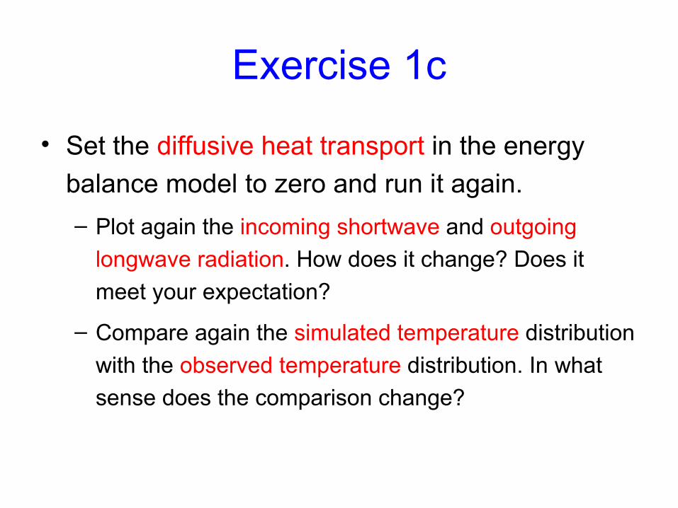
Exercise 1c

• Set the diffusive heat transport in the energy balance model to zero and run it again.– Plot again the incoming shortwave and outgoing

longwave radiation. How does it change? Does it meet your expectation?

– Compare again the simulated temperature distribution with the observed temperature distribution. In what sense does the comparison change?

What would be your experimental strategy to determine the influence of the greenhouse effect on the meridional temperature distribution?

Exercise 1d

Exercise 1d

• Restore the diffusive heat transport in the energy balance model; change the emissivity (say by 0.1) and run again.– Plot again the incoming shortwave and outgoing

longwave radiation. How does it change? Does it meet your expectation?

– Compare again the simulated temperature distribution with the observed temperature distribution. In what sense does the comparison change?

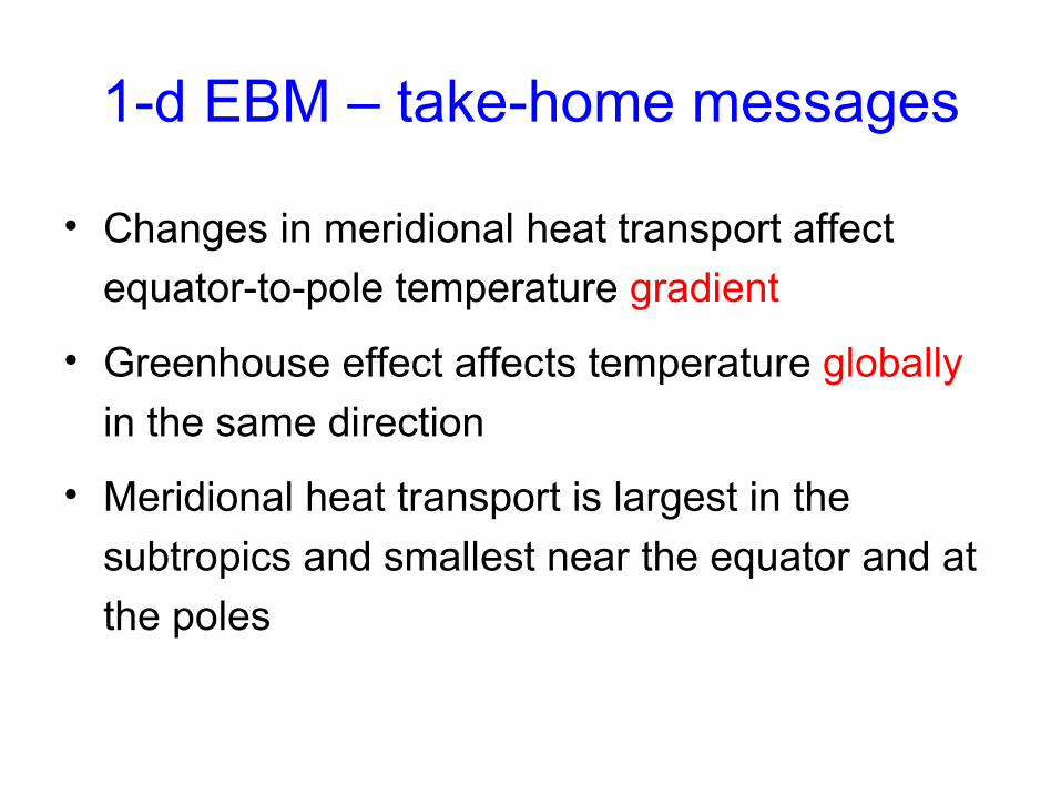
1-d EBM – take-home messages

• Changes in meridional heat transport affect equator-to-pole temperature gradient

• Greenhouse effect affects temperature globally in the same direction

• Meridional heat transport is largest in the subtropics and smallest near the equator and at the poles

“Supplementary material”

Exercise 2: Implementing the ice-albedo Feedback

• In time loop: set planetary albedo to 0.7 whenever temperature falls below -2°C (otherwise use the existing latitude-dependent formulation)

• Start by copying ebm_1d.m to ebm_1d_icealb.m

Within Time Loop:

for j=2:jmt-1 % Compute shortwave radiation budget netswpln(j) = solin(j)*(1.0 - apln(j));end

[snip]

%---------------------------------------------------------------% Step atmospheric temperature forward in time %---------------------------------------------------------------for j=2:jmt-1 tatm(j) = tatm(j) + dt*yp(j);end

Within Time Loop:

for j=2:jmt-1 % set temperature-dependent albedo if tatm(j) <= -2.0 apln(j) = 0.7; else apln(j) = 0.6 - 0.4*cst(j); end % Compute shortwave radiation budget netswpln(j) = solin(j)*(1.0 - apln(j));end

[snip]

%---------------------------------------------------------------% Step atmospheric temperature forward in time %---------------------------------------------------------------for j=2:jmt-1 tatm(j) = tatm(j) + dt*yp(j);end

Running the modified model

• Change min. temperature for plotting from -10 to -60

% Initialize plot…p1=plot(0,100,'.','EraseMode','none');set(p1,'linewidth',2);axis([0.6 1.3 -60 40]);

• Run ebm_1d_icealb.m

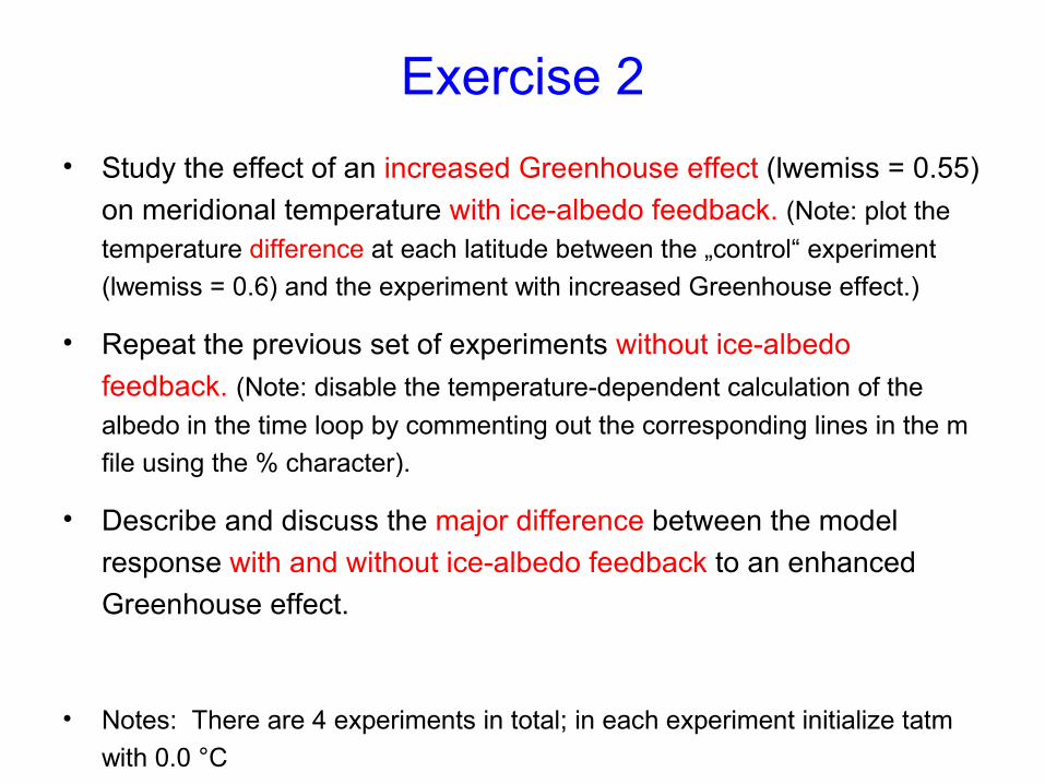
Exercise 2• Study the effect of an increased Greenhouse effect (lwemiss = 0.55)

on meridional temperature with ice-albedo feedback. (Note: plot the temperature difference at each latitude between the „control“ experiment (lwemiss = 0.6) and the experiment with increased Greenhouse effect.)

• Repeat the previous set of experiments without ice-albedo feedback. (Note: disable the temperature-dependent calculation of the albedo in the time loop by commenting out the corresponding lines in the m file using the % character).

• Describe and discuss the major difference between the model response with and without ice-albedo feedback to an enhanced Greenhouse effect.

• Notes: There are 4 experiments in total; in each experiment initialize tatm with 0.0 °C

• Hints to make the analysis easier:– Plot temperature difference (or “anomaly”)

• Note that calculated points are from 2 through jmt-1, end points are boundaries.

• Lower lwemiss means higher greenhouse effect.• There is no ice-albedo feedback above -2°C.

– Plot temperature differences with and without ice-albedo feedback in one plot

Ice-albedo feedback amplifies Greenhouse effect in high latutides “polar amplification”

Climate feedbacks – key points

• Feedbacks can make the response to climate forcings (highly) non-linear

• Feedbacks lead to threshold behavior in the climate system (climatic “surprises”)

• Ice-albedo feedback amplifies the greenhouse effect at high latitudes (“polar amplification”)

Final remarks on 1-d EBM

• Absorbed shortwave radiation– Includes annual-mean solar distribution function and planetary

albedo as a function of latitude and temperature

– What could be improved:• Include effect of changes in cloud cover

• Include scattering

• Add seasonal or diurnal cycle, etc.

• Outgoing longwave radition– “Gray body” approximation only, emissivity should at least be

different for atmosphere and ocean, etc.