One-day outdoor photometric stereo via skylight estimation

Jiyoung Jung Joon-Young Lee In So KweonRobotics and Computer Vision Lab, KAIST

{jyjung,jylee}@rcv.kaist.ac.kr iskweon77@kaist.ac.kr

Abstract

We present an outdoor photometric stereo method us-ing images captured in a single day. We simulate a skyhemisphere for each image according to its GPS and times-tamp, and parameterize the obtained sky hemisphere intoa quadratic skylight and a Gaussian sunlight distribution.Unlike previous works which usually model outdoor illu-mination as a sum of constant ambient light and a distantpoint light, our method models natural illumination accord-ing to a popular sky model and thus provides sufficient con-straints for shape reconstruction from one day images. Wegenerate pixel profiles of uniformly sampled unit vectors forthe corresponding time of captures and evaluate them usingcorrelation with the actual pixel profiles. The estimated sur-face normal is refined by MRF optimization. We have testedour method to recover objects and scenes of various sizes inreal-world outdoor daylight.

1. Introduction3D reconstruction of the scene from images has drawn

interests from many researchers in computer vision fordecades. There are several 3D reconstruction methods usingmore than two images such as multi-view stereo using im-ages from different viewpoints [6], photometric stereo usingimages under different light directions [38], and depth fromfocus [7] and defocus [36] using images with different fo-cal settings. There have been successful approaches using asingle image as well, such as shape from shading [9], withappropriate assumptions and constraints.

The related experiments were originally conducted in-side the lab where the equipments and environments canbe controlled. Then the methods have been improved toovercome the difficulties of uncontrolled elements one byone. For example, multi-view stereo has been evolved fromusing images captured by uniformly placed cameras in thelab [25] to searching and downloading images of the sceneof interest from the web [4]. The results are promising eventhough the input images are taken from different cameras indifferent time, viewpoints, and many other conditions.

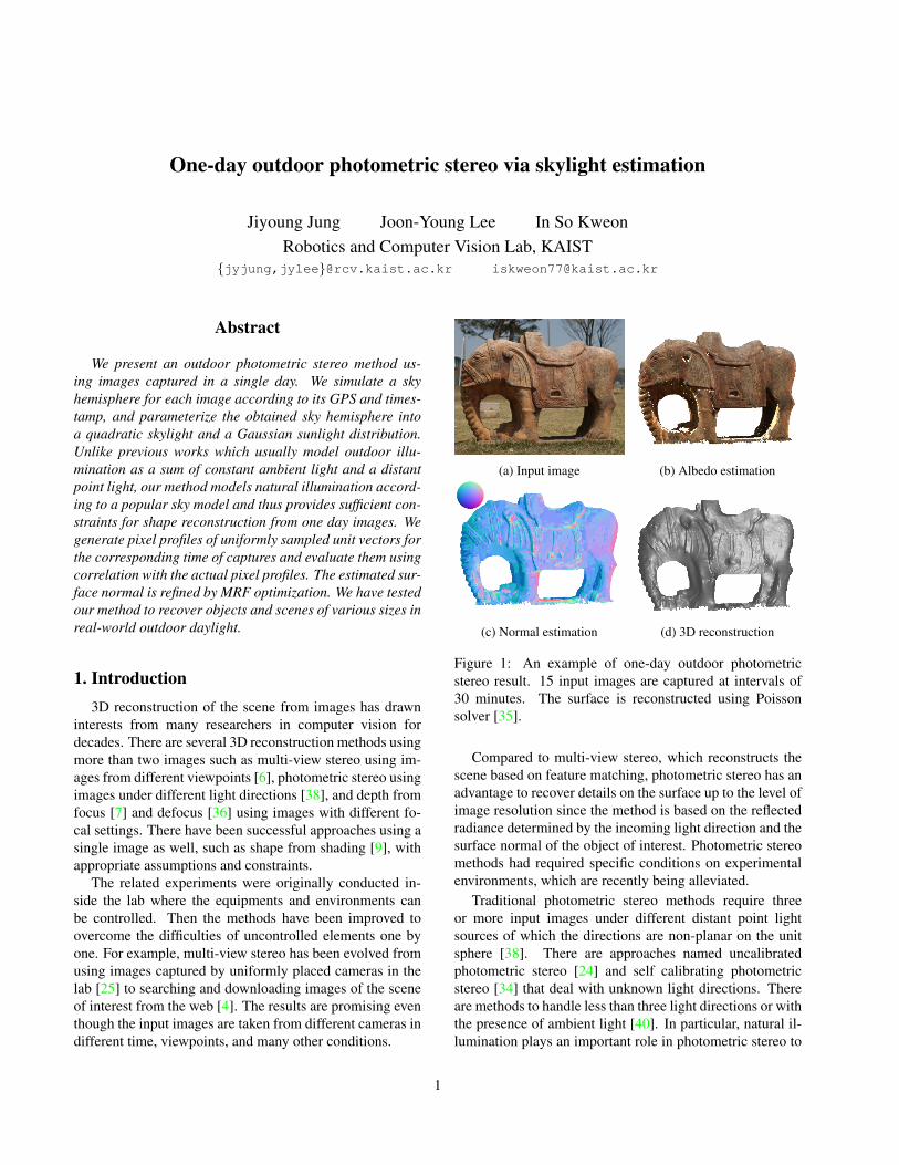
(a) Input image (b) Albedo estimation

(c) Normal estimation (d) 3D reconstruction

Figure 1: An example of one-day outdoor photometricstereo result. 15 input images are captured at intervals of30 minutes. The surface is reconstructed using Poissonsolver [35].

Compared to multi-view stereo, which reconstructs thescene based on feature matching, photometric stereo has anadvantage to recover details on the surface up to the level ofimage resolution since the method is based on the reflectedradiance determined by the incoming light direction and thesurface normal of the object of interest. Photometric stereomethods had required specific conditions on experimentalenvironments, which are recently being alleviated.

Traditional photometric stereo methods require threeor more input images under different distant point lightsources of which the directions are non-planar on the unitsphere [38]. There are approaches named uncalibratedphotometric stereo [24] and self calibrating photometricstereo [34] that deal with unknown light directions. Thereare methods to handle less than three light directions or withthe presence of ambient light [40]. In particular, natural il-lumination plays an important role in photometric stereo to

1

come out of controlled environments [10, 14]. Reflectanceand shape of an object are recovered from the illuminationmap with complex light information around the object [26]and analogously the illumination map and reflectance arerecovered using an object with known shape [23]. Recently,fusing shape-from-shading with a depth sensor alleviatesmany assumptions and shows promising results [8, 16, 39].

So far, an outdoor environment has been regarded as fullof unknowns and complexities. The appearance of an openfield changes drastically depending on its weather conditionand time of day, but at the same time, it does have a generalappearance. While the appearance of a room can easily beinfluenced by which kind of light we turn on, an outdoorfield on a clear day presents a relatively predictable scene.

In this work, we present an outdoor photometric stereomethod based on the motivation that the outdoor illumina-tion which is mainly contributed by the sun and clear skycan be generally modeled. We process geo-tagged, time-stamped images captured from a static camera in a singleday to estimate the surface normal of the scene. There arethree major contributions of this work. First, we adapt theskylight distribution [28] to work for outdoor photometricstereo without any depth priors of the scene. Second, weovercome the weak rank-3 qualification of sunlight direc-tions during a single day by exploiting natural illuminationvia skylight estimation. Finally, since we deal with a hand-ful of images, there exist pixels lit by the sun in less thantwo images. Incomplete surface normal estimation for thesepixels are refined using information from their neighboringpixels of similar profiles through MRF optimization.

2. Related workThere have been several approaches for outdoor photo-

metric stereo in recent years. Ackermann et al. [3] andAbrams et al. [1] use time-lapse sequences captured bystatic outdoor webcams. Since both approaches model theillumination as a distant point light (the sun) with a con-stant ambient light, they require many months of images toavoid coplanar light directions in photometric stereo. Theyundergo image selection to remove images of bad weatherand night time and process hundreds of selected images.Abrams et al. [1] propose an iterative, non-linear optimiza-tion of ambient light, shadows, light color, surface normals,radiometric calibration, and exposures. It is a huge op-timization using 500 images of careful selection. Acker-mann et al. [3] present a process of image filtering and se-lection to find 50 proper images from 20k candidate images.

Shan et al. [32] present large-scale reconstruction and re-lighting results using hundreds of thousands of images fromvarious sources through structure-from-motion, multi-viewstereo, and surface reconstruction. They select cloudy im-ages first to estimate albedo and ambient light, then sunnyimages to estimate light including a distant point light per

image and to refine the surface normal of the scene.While a point light source with a constant ambient light

are shown to be an effective way of modeling outdoor en-vironment with the help of large amount of observations ordepth priors, we paid attention to the complexity of naturalillumination being an aid rather than hindrance to the gen-eral shape-from-shading problems, as in [14]. Since out-door scenes are covered with sky by definition, there areresearches that utilize the sky as a source of information fordiverse purposes.

Sunkavalli et al. [37] assume that the subspace contain-ing daylight spectra is two-dimensional and propose a colormodel for the temporal color changes of outdoor image se-quences. Lalonde et al. [21] recover camera parameters in-cluding its focal length and pose from the sun position ora part of clear sky in the image with time and location ofthe capture. The same group estimates the natural illumi-nation conditions from a single image using sky model andinserts a virtual object into the image so that it looks nat-ural under the estimated illumination [20]. Kawakami etal. [17] compare the sky image with the sky model to esti-mate camera spectral sensitivity and white balance setting.Inose et al. [12] refine the multi-view stereo result of an out-door scene by using one day images for photometric stereo.The sky model is incorporated to seperate the effect of thesun and sky illumination onto the surface.

Shen et al. [33] present an interesting analysis on thestability of the photometric stereo problem using one-dayimages. As the earth revolves around the sun, the angleof declination varies from 0 to 23 degrees which leads tonon-planar sunlight directions in certain days of the year.They calculated the inverse of the condition number (ra-tio of minimum to maximum eigenvalues) of the light di-rection matrix per day, for varying latitude and date. Forlimited cases, the light direction matrix does suffice rank-3constraint, but with a small inverse condition number. Thisanalysis shows the limitation of the point light source mod-eling of one day outdoor photometric stereo and thereforewe seek for promising solution in natural illumination us-ing skylight estimation.

3. Sky appearanceSkylight is a non-uniform extended light source whose

intensity and angular distribution pattern varies as a func-tion of insolation conditions [27]. Daylight environment es-timation requires sky luminance angular distribution, whichis more complex than a direct sunlight plus a constantbrightness.

3.1. Sky luminance and chromaticity

The sky model proposed by Perez et al. [27] describesthe luminance of any arbitrary sky element as a function ofits elevation, and its relative orientation with respect to the

𝜃𝜃

𝛾𝛾

𝜙𝜙𝑠𝑠 𝑥𝑥(𝐸𝐸𝐸𝐸𝑠𝑠𝐸𝐸)

𝑦𝑦(𝑁𝑁𝑁𝑁𝑁𝑁𝐸𝐸𝑁)

𝑧𝑧(𝑈𝑈𝑈𝑈)

𝑉𝑉𝑉𝑉𝑉𝑉𝑉𝑉

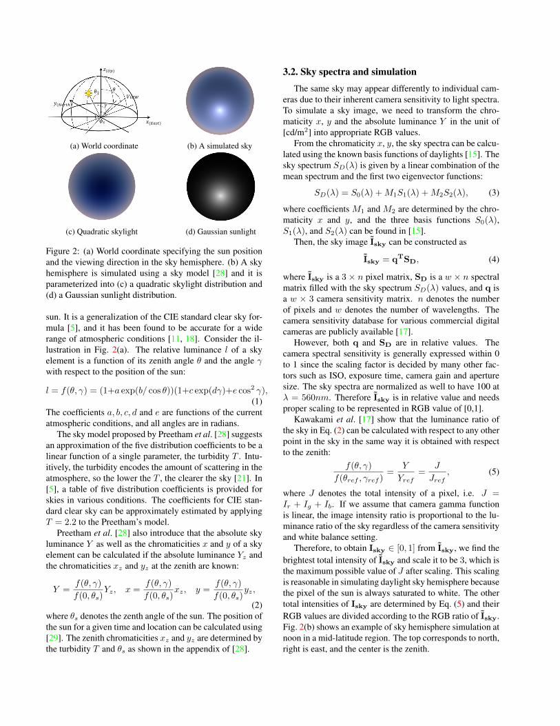
(a) World coordinate (b) A simulated sky

(c) Quadratic skylight (d) Gaussian sunlight

Figure 2: (a) World coordinate specifying the sun positionand the viewing direction in the sky hemisphere. (b) A skyhemisphere is simulated using a sky model [28] and it isparameterized into (c) a quadratic skylight distribution and(d) a Gaussian sunlight distribution.

sun. It is a generalization of the CIE standard clear sky for-mula [5], and it has been found to be accurate for a widerange of atmospheric conditions [11, 18]. Consider the il-lustration in Fig. 2(a). The relative luminance l of a skyelement is a function of its zenith angle θ and the angle γwith respect to the position of the sun:

l = f(θ, γ) = (1+a exp(b/ cos θ))(1+c exp(dγ)+e cos2 γ),(1)

The coefficients a, b, c, d and e are functions of the currentatmospheric conditions, and all angles are in radians.

The sky model proposed by Preetham et al. [28] suggestsan approximation of the five distribution coefficients to be alinear function of a single parameter, the turbidity T . Intu-itively, the turbidity encodes the amount of scattering in theatmosphere, so the lower the T , the clearer the sky [21]. In[5], a table of five distribution coefficients is provided forskies in various conditions. The coefficients for CIE stan-dard clear sky can be approximately estimated by applyingT = 2.2 to the Preetham’s model.

Preetham et al. [28] also introduce that the absolute skyluminance Y as well as the chromaticities x and y of a skyelement can be calculated if the absolute luminance Yz andthe chromaticities xz and yz at the zenith are known:

Y =f(θ, γ)

f(0, θs)Yz, x =

f(θ, γ)

f(0, θs)xz, y =

f(θ, γ)

f(0, θs)yz,

(2)where θs denotes the zenth angle of the sun. The position ofthe sun for a given time and location can be calculated using[29]. The zenith chromaticities xz and yz are determined bythe turbidity T and θs as shown in the appendix of [28].

3.2. Sky spectra and simulation

The same sky may appear differently to individual cam-eras due to their inherent camera sensitivity to light spectra.To simulate a sky image, we need to transform the chro-maticity x, y and the absolute luminance Y in the unit of[cd/m2] into appropriate RGB values.

From the chromaticity x, y, the sky spectra can be calcu-lated using the known basis functions of daylights [15]. Thesky spectrum SD(λ) is given by a linear combination of themean spectrum and the first two eigenvector functions:

SD(λ) = S0(λ) +M1S1(λ) +M2S2(λ), (3)

where coefficients M1 and M2 are determined by the chro-maticity x and y, and the three basis functions S0(λ),S1(λ), and S2(λ) can be found in [15].

Then, the sky image Isky can be constructed as

Isky = qTSD, (4)

where Isky is a 3 × n pixel matrix, SD is a w × n spectralmatrix filled with the sky spectrum SD(λ) values, and q isa w × 3 camera sensitivity matrix. n denotes the numberof pixels and w denotes the number of wavelengths. Thecamera sensitivity database for various commercial digitalcameras are publicly available [17].

However, both q and SD are in relative values. Thecamera spectral sensitivity is generally expressed within 0to 1 since the scaling factor is decided by many other fac-tors such as ISO, exposure time, camera gain and aperturesize. The sky spectra are normalized as well to have 100 atλ = 560nm. Therefore Isky is in relative value and needsproper scaling to be represented in RGB value of [0,1].

Kawakami et al. [17] show that the luminance ratio ofthe sky in Eq. (2) can be calculated with respect to any otherpoint in the sky in the same way it is obtained with respectto the zenith:

f(θ, γ)

f(θref , γref )=

Y

Yref=

J

Jref, (5)

where J denotes the total intensity of a pixel, i.e. J =Ir + Ig + Ib. If we assume that camera gamma functionis linear, the image intensity ratio is proportional to the lu-minance ratio of the sky regardless of the camera sensitivityand white balance setting.

Therefore, to obtain Isky ∈ [0, 1] from Isky, we find thebrightest total intensity of Isky and scale it to be 3, which isthe maximum possible value of J after scaling. This scalingis reasonable in simulating daylight sky hemisphere becausethe pixel of the sun is always saturated to white. The othertotal intensities of Isky are determined by Eq. (5) and theirRGB values are divided according to the RGB ratio of Isky.Fig. 2(b) shows an example of sky hemisphere simulation atnoon in a mid-latitude region. The top corresponds to north,right is east, and the center is the zenith.

3.3. Skylight parameterization

We separate the simulated sky hemisphere in Fig. 2(b)into a dominant sunlight and a diffuse skylight to modelshadowed and non-shadowed pixels. A point in the scene isilluminated by all the rays coming from the hemisphere de-termined by its surface normal. The shadowed pixel mainlyappears when its hemisphere does not contain the sun (selfshadow) or if the sun is occluded (cast shadow). The re-sulting shadowed pixel is illuminated by a part of the skywithout the sun.

Since it is difficult to distinguish if the shadow is selfshadow or cast shadow, we model every shadowed pixel tobe illuminated by the hemisphere determined by its surfacenormal excluding the sunlight. This method has two advan-tages over the constant ambient light modeling. One is thatit models the ambient light to vary according to the surfacenormal and the skylight distribution, which is physicallyplausible. The other is the illumination ratio between theskylight and the sunlight for a pixel is already determined,and leave us only one scaling factor to disambiguate, whichis albedo. This removes the ambiguity between the ambi-ent and direct illumination and therefore makes the problemmore constrained.

Given the simulated skylight for every angle of the skyhemisphere, we make it grayscale and fit a Gaussian func-tion of the angle γ with respect to the known sun position.Then we subtract the hemisphere containing only the Gaus-sian sunlight from the original sky hemisphere and modelthe rest of the sky using a quadratic function with respect tothe sky orientation as a shading equation in [14].

Lsky(sk) = sTkAqsk + bTq sk + cq, (6)

Lsun(γ) = ag exp(−((γ − bg)/cg)2), (7)

where sk is the direction of a sky element k, which can bedefined by the angle γ with respect to the position of thesun as in Fig. 2(a). The parameters of the quadratic func-tion are composed of a symmetric matrix Aq ∈ R3×3, avector bq ∈ R3×1 and a constant cq ∈ R. The quadraticskylight distribution Lsky and the Gaussian sunlight distri-bution Lsun are shown in Fig. 2(c) and (d), respectively.

The proposed parametric model represents the sky hemi-sphere effectively. In addition, it leaves open the possibilityfor optimizing the skylight parameters in the future.

4. Image formationThe imaged appearance I(x) at a given pixel x de-

pends on the surface orientation nx. The orientation deter-mines the hemisphere of light that is visible at that location.The material Ψ determines how this light is integrated toform the observed appearance [26]. Therefore, the light-ing environment and the material form reflected radiance

RΨ(nx,L) that gives the appearance for a given surfaceorientation.

The reflected radiance is computed by integrating the in-cident irradiance E modulated by the reflectance over theillumination L,

RΨ(nx,L) =

∫ρ(ωi, ωo; Ψ)L(ωi) max(0,nx · ωi)dωi,

(8)

E(nx,L) =

∫L(ωi) max(0,nx · ωi)dωi, (9)

where ωi and ωo are the incident and outgoing (viewing) an-gles of the light on the surface [26]. Assuming Lambertianreflectance, albedo ρ is invariant to the viewing direction.Therefore, we model the pixel intensity of each color chan-nel to be proportional to the incident irradiance E on thesurface by the albedo.

I(x) = Isky(x) + S(x)Isun(x), (10)

Ic(x) = ρc(x)(E(nx,Lsky) + S(x)E(nx,Lsun)), (11)

where c denotes a color channel and S(x) is a binary valuewhich indicates the pixel x is in shadow. The equationshold independently for each input image t, but we omit thesubscript for simplicity.

Using the simulated sky hemisphere as an illuminationmap, we calculate the incident irradiance for uniformlysampled unit vectors, as Eq. (9). The incident irradiancedue to skylight illumination Lsky and sunlight illuminationLsun are computed separately. For each pixel, the estimatedshadow mask S(x) is applied to sum those two incident ir-radiances as Eq. (11). The incident irradiance values for allthe input images are stacked to be a profile for each sam-ple unit vector. These sample profiles in the dimension ofthe number of images are compared with the actual pixelprofiles.

5. Surface normal and albedo estimationIn this section, we present a framework for outdoor pho-

tometric stereo using the estimated natural illumination thatconsists of skylight and sunlight distribution. We detect theshadowed pixels explicitly and estimate the initial (relative)albedo using the color ratio. The surface normal is esti-mated using the correlation between the pixel profile andthe sample profiles generated according to the image for-mation model. The (absolute) albedo is updated and thenthe surface normal is refined by MRF optimization.

5.1. Shadow detection

We detect the shadowed pixels explicitly using theshadow estimation method for [2]. This method is an expec-tation maximization approach which simultaneously esti-mates shadows, albedo, surface normals, and ambient light.

Unlike previous shadow detection procedures, this methoduse the sunlight directions and solves for the shadows thatare most consistent with a Lambertian assumption.

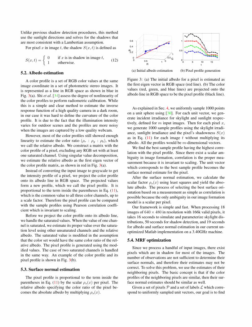
For pixel x in image t, the shadow S(x, t) is defined as

S(x, t) =

{0 if x is in shadow in image t,1 otherwise. (12)

5.2. Albedo estimation

A color profile is a set of RGB color values at the sameimage coordinate in a set of photometric stereo images. Itis represented as a line in RGB space as shown in blue inFig. 3(a). Shi et al. [34] assess the degree of nonlinearity ofthe color profiles to perform radiometric calibration. Whilethis is a simple and clear method to estimate the inverseresponse function of a high quality camera in a dark room,in our case it was hard to define the curvature of the colorprofile. It is due to the fact that the illumination intensityvaries for outdoor scenes and the profiles are more noisywhen the images are captured by a low quality webcam.

However, most of the color profiles still showed enoughlinearity to estimate the color ratio (ρr : ρg : ρb), whichwe call the relative albedo. We construct a matrix with thecolor profile of a pixel, excluding any RGB set with at leastone saturated channel. Using singular value decomposition,we estimate the relative albedo as the first eigen vector ofthe color profile matrix, as shown in red in Fig. 3(a).

Instead of converting the input image to grayscale to getthe intensity profile of a pixel, we project the color profileonto its albedo line in RGB space. The projected valuesform a new profile, which we call the pixel profile. It isproportional to the term inside the parentheses in Eq. (11),which is the common value to all three color channels, up toa scale factor. Therefore the pixel profile can be comparedwith the sample profiles using Pearson correlation coeffi-cient which is invariant to scaling.

Before we project the color profile onto its albedo line,we handle the saturated values. When the value of one chan-nel is saturated, we estimate its proper value over the satura-tion level using other unsaturated channels and the relativealbedo. The saturated value is modified in the assumptionthat the color set would have the same color ratio of the rel-ative albedo. The pixel profile is generated using the mod-ified values. The case of two saturated channels is handledin the same way. An example of the color profile and itspixel profile is shown in Fig. 3(b).

5.3. Surface normal estimation

The pixel profile is proportional to the term inside theparentheses in Eq. (11) by the scalar ρs(x) per pixel. Therelative albedo specifying the color ratio of the pixel be-comes the absolute albedo by multiplying ρs(x).

(a) Initial albedo estimation (b) Pixel profile generation

Figure 3: (a) The initial albedo for a pixel is estimated asthe first eigen vector in RGB space (red line). (b) The colorvalues (red, green, and blue lines) are projected onto thealbedo line in RGB space to be the pixel profile (black line).

As explained in Sec. 4, we uniformly sample 1000 pointson a unit sphere using [30]. For each unit vector, we gen-erate incident irradiance for skylight and sunlight respec-tively, defined for m input images. Then for each pixel x,we generate 1000 sample profiles using the skylight irradi-ance, sunlight irradiance and the pixel’s shadowness S(x)as in Eq. (11) for each image t without multiplying itsalbedo. All the profiles would be m-dimensional vectors.

We find the best sample profile having the highest corre-lation with the pixel profile. Since there exist a scalar am-biguity in image formation, correlation is the proper mea-surement because it is invariant to scaling. The unit vectorwhich corresponds to the best sample profile becomes thesurface normal estimate for the pixel.

After the surface normal estimation, we calculate thescalar factor ρs(x) using least squares and yield the abso-lute albedo. The process of selecting the best surface ori-entation based on a measurement as simple as correlation ispossible because the only ambiguity in our image formationmodel is a scalar per pixel.

Our framework is simple and fast. When processing 18images of 640× 480 in resolution with 166k valid pixels, ittakes 16 seconds to simulate and parameterize skylight dis-tributions, 50 seconds for shadow detection, and 19 secondsfor albedo and surface normal estimation in our current un-optimized Matlab implementation on a 3.40GHz machine.

5.4. MRF optimization

Since we process a handful of input images, there existpixels which are in shadow for most of the images. Thenumber of observations are not sufficient to determine theirsurface normals, and therefore their estimates may not becorrect. To solve this problem, we use the estimates of theirneighboring pixels. The basic concept is that if the colorprofiles of the neighboring pixels are similar, then their sur-face normal estimates should be similar as well.

Given a set of pixels P and a set of labels L which corre-spond to uniformly sampled unit vectors, our goal is to find

a labeling l (i.e. a mapping from P to sample orientationsL) which minimizes the following energy function:

E(l) =∑p∈P

Dp(lp) +∑

p,q∈NVp,q(lp, lq), (13)

where N ⊂ P × P is a neighborhood system on pixels.Dp(lp) is a data term that measures the cost of assigningulp as the surface normal of the pixel p. Vp,q(lp, lq) is asmoothness term that measures the cost of assigning ulp ,ulq to the adjacent pixels p, q.

Dp(lp) = 1− corr(SP (lp, p), PP (p)), (14)

Vp,q(lp, lq)=∑

c=R,G,B

(1 + corr(Ic(p), Ic(q)))(1− uTlpulq ),

(15)where corr(a, b) denotes the Pearson correlation coefficientof two profiles a and b, SP (l, p) denotes the sample profileof the unit vector ul using the shadow mask of pixel p, andPP (p) denotes the pixel profile of p. Here Ic(p) denotes thecolor profile of p for all the images. We perform multi-labeloptimization using graph cut [19] to seek the set of surfaceorientations that minimizes the energy E(l).

6. ResultsWe demonstrate our approach on five real-world

datasets. We captured Elephant and Cicero datasets on twodifferent days using the same Canon 5D Mark III camera.Each set contains 15 images taken at intervals of 30 min-utes. We tested our algorithm on Dusseldorf, Meersburg,and Arizona datasets from the AMOS webcam archive [13].We manually selected sunny days from the available imagesand processed 18 images or less for each set.

In the experiments, we assume that the scene has Lam-bertian reflectance and that the image intensities are linearto the scene radiance except for the saturated intensities. Wedid not include an explicit radiometric calibration processto the framework due to its unstable outcome. However,we believe any existing radiometric calibration method suchas [22] with proper modification may improve the perfor-mance of our method.

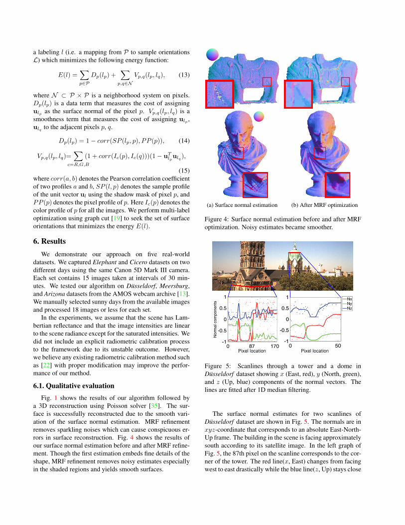
6.1. Qualitative evaluation

Fig. 1 shows the results of our algorithm followed bya 3D reconstruction using Poisson solver [35]. The sur-face is successfully reconstructed due to the smooth vari-ation of the surface normal estimation. MRF refinementremoves sparkling noises which can cause conspicuous er-rors in surface reconstruction. Fig. 4 shows the results ofour surface normal estimation before and after MRF refine-ment. Though the first estimation embeds fine details of theshape, MRF refinement removes noisy estimates especiallyin the shaded regions and yields smooth surfaces.

(a) Surface normal estimation (b) After MRF optimization

Figure 4: Surface normal estimation before and after MRFoptimization. Noisy estimates became smoother.

Figure 5: Scanlines through a tower and a dome inDusseldorf dataset showing x (East, red), y (North, green),and z (Up, blue) components of the normal vectors. Thelines are fitted after 1D median filtering.

The surface normal estimates for two scanlines ofDusseldorf dataset are shown in Fig. 5. The normals are inxyz-coordinate that corresponds to an absolute East-North-Up frame. The building in the scene is facing approximatelysouth according to its satellite image. In the left graph ofFig. 5, the 87th pixel on the scanline corresponds to the cor-ner of the tower. The red line(x, East) changes from facingwest to east drastically while the blue line(z, Up) stays close

to zero since both faces are vertical. A peak at the 40th pixelcorresponds to the arch on the wall. The red line in the rightgraph of Fig. 5 shows slightly discontinuous structure of thedome in the scene.

In Fig. 6 and Fig. 7, we compare our performance withtwo previous methods. Fig. 7 shows the albedo and surfacenormal estimation of our method using one-day images ofDusseldorf and Meersburg datasets. The shadow detectionmethod for [2] which also estimates albedo, surface nor-mals, and ambient light is compared using the same oneday images. Abrams et al. [1]’s results using 500 imagesof many months are obtained from their original paper. Forcomparison, we used the same color map defined in theirpaper. Since the color coding is based on absolute East-North-Up coordinate, we indicate the color sphere of thecorresponding view point with the surface normal results.

It is shown that our method definitely outperforms othermethods using one day or even one month of images. Theillumination model of a point light source and a constantambient light shows severe performance degradation whenthe observations do not cover several months. On the otherhand, our modeling of natural illumination using skylightdistribution gives sufficient constraints from small numberof observations, and shows similar or better performancewith the previous method using 4 months of images.

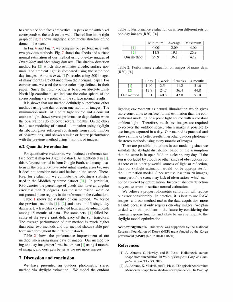
6.2. Quantitative evaluation

For quantitative evaluation, we obtained a reference sur-face normal map for Arizona dataset. As mentioned in [1],this reference normal is from Google Earth, and many loca-tions in the reference have substantial angular error becauseit does not consider trees and bushes in the scene. There-fore, for evaluation, we compute the robustness statisticsused in the Middlebury stereo dataset [31]. In particular,R30 denotes the percentage of pixels that have an angularerror less than 30 degrees. For the same reason, we ruledout ground plane regions in the reference in the evaluation.

Table 1 shows the stability of our method. We testedthe previous methods [1], [2] and ours on 15 single-daydatasets. Each set(day) is selected from an individual monthamong 15 months of data. For some sets, [1] failed be-cause of the severe rank deficiency of the sun trajectory.The average performance of our method is much higherthan other two methods and our method shows stable per-formance throughout the different datasets.

Table 2 shows the performance improvement of ourmethod when using many days of images. Our method us-ing one-day images performs better than [1] using 4 monthsof images, and ours gets better as we use more images.

7. Discussion and conclusionWe have presented an outdoor photometric stereo

method via skylight estimation. We model the outdoor

Table 1: Performance evaluation on fifteen different sets ofone-day images (R30) [%]

Minimum Average Maximum[1] 0.00 2.09 4.09[2] 11.8 19.1 25.9

Our method 29.9 36.1 42.2

Table 2: Performance evaluation on images of many days(R30) [%]

1 day 1 week 2 weeks 4 months[1] 1.40 2.54 11.2 31.6[2] 12.9 24.7 36.4 44.8

Our method 38.1 40.8 47.0 51.0

lighting environment as natural illumination which givesmore constraints to surface normal estimation than the con-ventional modeling of a point light source with a constantambient light. Therefore, much less images are requiredto recover the outdoor scene, which makes it possible touse images captured in a day. Our method is practical andshows similar or better results than other outdoor photomet-ric stereo methods using many months of images.

There are possible limitations in our modeling since wesimulate the skylight distribution based on the assumptionthat the scene is in open field on a clear sunny day. If thesun is occluded by clouds or other kinds of obstructions, orif there exist other powerful sources of light or reflection,then our skylight estimation would not be appropriate forthe illumination model. Since we use less than 20 images,some part of the scene may lack of observations which can-not be covered by optimization. Incorrect shadow detectionmay cause errors in surface normal estimation.

We believe a proper radiometric calibration will reduceour error considerably. In practice, it is best to use RAWimages, and our method makes the data acquisition morefeasible because it only requires one-day images. We planto deal with this problem in the future by considering thecamera response function and white balance setting into theskylight model optimization.

Acknowledgements. This work was supported by the NationalResearch Foundation of Korea (NRF) grant funded by the Koreagovernment (MSIP) (No. 2010-0028680).

References[1] A. Abrams, C. Hawley, and R. Pless. Heliometric stereo:

shape from sun position. In Proc. of European Conf. on Com-puter Vision (ECCV), 2012.

[2] A. Abrams, K. Miskell, and R. Pless. The episolar constraint:Monocular shape from shadow correspondence. In Proc. of

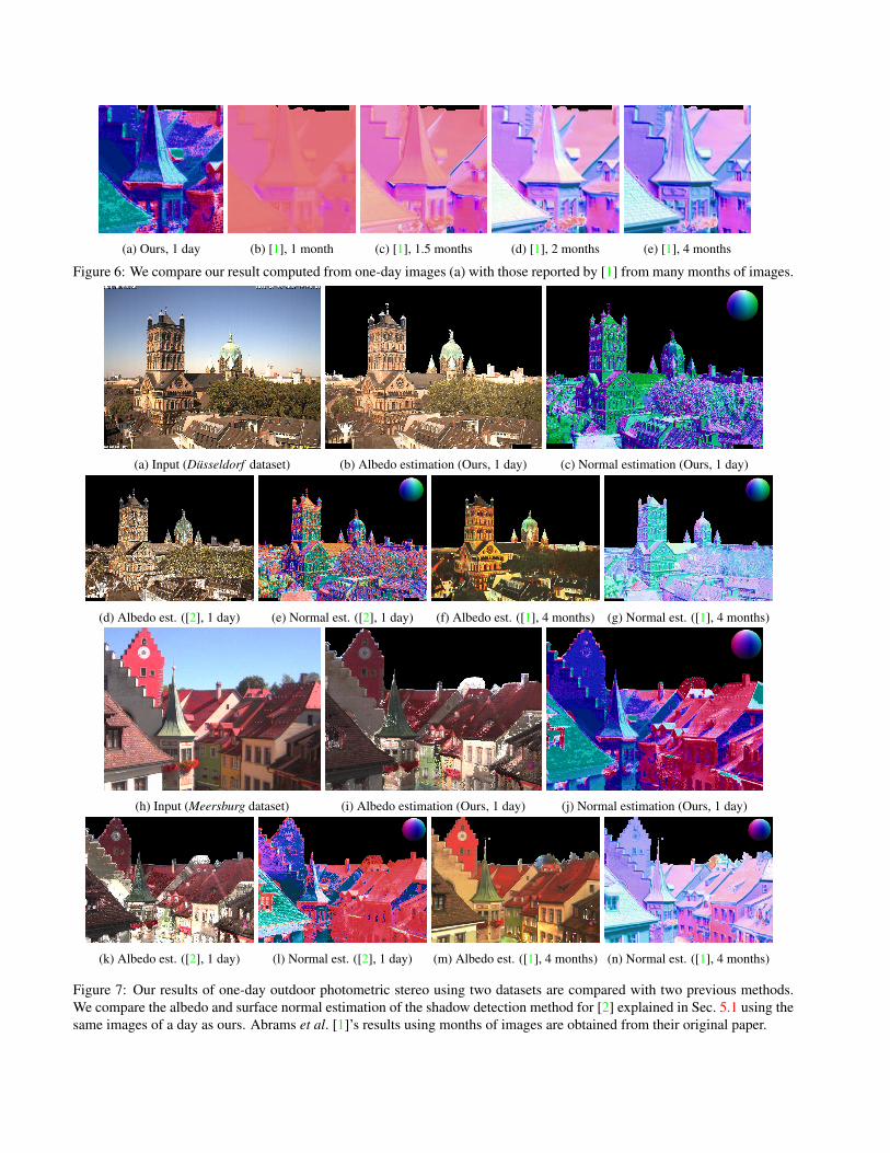
(a) Ours, 1 day (b) [1], 1 month (c) [1], 1.5 months (d) [1], 2 months (e) [1], 4 months

Figure 6: We compare our result computed from one-day images (a) with those reported by [1] from many months of images.

(a) Input (Dusseldorf dataset) (b) Albedo estimation (Ours, 1 day) (c) Normal estimation (Ours, 1 day)

(d) Albedo est. ([2], 1 day) (e) Normal est. ([2], 1 day) (f) Albedo est. ([1], 4 months) (g) Normal est. ([1], 4 months)

(h) Input (Meersburg dataset) (i) Albedo estimation (Ours, 1 day) (j) Normal estimation (Ours, 1 day)

(k) Albedo est. ([2], 1 day) (l) Normal est. ([2], 1 day) (m) Albedo est. ([1], 4 months) (n) Normal est. ([1], 4 months)

Figure 7: Our results of one-day outdoor photometric stereo using two datasets are compared with two previous methods.We compare the albedo and surface normal estimation of the shadow detection method for [2] explained in Sec. 5.1 using thesame images of a day as ours. Abrams et al. [1]’s results using months of images are obtained from their original paper.

CVPR, 2013.[3] J. Ackermann, F. Langguth, S. Fuhrmann, and M. Goesele.

Photometric stereo for outdoor webcams. In Proc. of CVPR,2012.

[4] S. Agarwal, Y. Furukawa, N. Snavely, I. Simon, B. Curless,and S. M. Seitz. Building rome in a day. Communications ofthe ACM, 54(10):105–112, 2011.

[5] C. T. Committee. Spatial distribution of daylight–CIE stan-dard general sky. Technical report, International Commis-sion on Illumination, 2002.

[6] Y. Furukawa and J. Ponce. Accurate, dense, and robust multi-view stereopsis. IEEE Trans. on Pattern Analysis and Ma-chine Intelligence (PAMI), 32(8):1362–1376, 2010.

[7] P. Grossmann. Depth from focus. Pattern Recognition Let-ters, 5(1):63–69, 1987.

[8] Y. Han, J.-Y. Lee, and I. S. Kweon. High quality shape froma single RGB-D image under uncalibrated natural illumina-tion. In Proc. of Int’l Conf. on Computer Vision (ICCV),2013.

[9] B. K. P. Horn. Shape from shading. chapter Obtaining Shapefrom Shading Information, pages 123–171. MIT Press, Cam-bridge, MA, USA, 1989.

[10] R. Huang and W. A. P. Smith. Shape-from-shading undercomplex natural illumination. In Proc. of Int’l Conf. on Im-age Processing (ICIP), 2011.

[11] P. Ineichen, B. Molineaux, and R. Perez. Sky luminancedata validation: comparison of seven models with four databanks. Solar Energy, 52(4):337–346, 1994.

[12] K. Inose, S. Shimizu, R. Kawakami, Y. Mukaigawa, andK. Ikeuchi. Refining outdoor photometric stereo based onsky model. IPSJ Trans. on Computer Vision and Applica-tions, 5(1):104–108, 2013.

[13] N. Jacobs, N. Roman, and R. Pless. Consistent temporalvariations in many outdoor scenes. In Proc. of CVPR, 2007.

[14] M. K. Johnson and E. H. Adelson. Shape estimation in nat-ural illumination. In Proc. of CVPR, 2011.

[15] D. B. Judd, D. L. MacAdam, and G. Wyszecki. Spectraldistribution of typical daylight as a function of correlatiedcolor temperature. Journal of the Optical Society of America,54(8):1031–1036, 1964.

[16] J. Jung, J.-Y. Lee, Y. Jeong, and I. S. Kweon. Time-of-flightsensor calibration for a color and depth camera pair. IEEETrans. on Pattern Analysis and Machine Intelligence (PAMI).

[17] R. Kawakami, H. Zhao, R. T. Tan, and K. Ikeuchi. Cam-era spectral sensitivity and white balance estimation fromsky images. Int’l Journal of Computer Vision (IJCV),105(3):187–204, 2013.

[18] J. T. Kider, Jr., D. Knowlton, J. Newlin, Y. K. Li, and D. P.Greenberg. A framework for the experimental comparisonof solar and skydome illumination. ACM Trans. on Graphics(TOG), 33(6):180:1–180:12, Nov. 2014.

[19] V. Kolmogorov and R. Zabih. What energy functions can beminimized via graph cuts? IEEE Trans. on Pattern Analysisand Machine Intelligence (PAMI), 26(2):147–159, 2004.

[20] J.-F. Lalonde, A. A. Efros, and S. G. Narasimhan. Estimat-ing natural illumination from a single outdoor image. Int’lJournal of Computer Vision (IJCV), 98(2):123–145, 2012.

[21] J.-F. Lalonde, S. G. Narasimhan, and A. A. Efros. What dothe sun and the sky tell us about the camera? Int’l Journal ofComputer Vision (IJCV), 88(1):24–51, 2010.

[22] J.-Y. Lee, Y. Matsushita, B. Shi, and I. S. Kweon. Radiomet-ric calibration by rank minimization. IEEE Trans. on PatternAnalysis and Machine Intelligence (PAMI), 35(1):114–156,2013.

[23] S. Lombardi and K. Nishino. Reflectance and illuminationfrom a single image. In Proc. of European Conf. on Com-puter Vision (ECCV), 2012.

[24] F. Lu, Y. Matsushita, I. Sato, T. Okabe, and Y. Sato.Uncalibrated photometric stereo for unknown isotropic re-flectances. In Proc. of CVPR, 2013.

[25] M. Okutomi and T. Kanade. A multiple-baseline stereo sys-tem. IEEE Trans. on Pattern Analysis and Machine Intelli-gence (PAMI), 15(4):353–363, 1993.

[26] G. Oxholm and K. Nishino. Shape and reflectance from nat-ural illumination. In Proc. of European Conf. on ComputerVision (ECCV), 2012.

[27] R. Perez, R. Seals, and J. Michalsky. All-weather model forsky luminance distribution–preliminary configuration andvalidation. Solar Energy, 50(3):235–245, 1993.

[28] A. J. Preetham, P. Shirley, and B. Smits. A practical analyticmodel for daylight. In Proc. of ACM SIGGRAPH, 1999.

[29] I. Reda and A. Andreas. Solar position algorithm for solar ra-diation application. Technical Report NREL/TP-560-34302,National Renewable Energy Laboratory (NREL), 2003.

[30] E. Saff and A. B. J. Kuijlaars. Distributing many points on asphere. The Mathematical Intelligencer, 19(1):5–11, 1997.

[31] D. Scharstein and R. Szeliski. A taxonomy and evaluationof dense two-frame stereo correspondence algorithms. Int’lJournal of Computer Vision (IJCV), 47(13):7–42, 2002.

[32] Q. Shan, R. Adams, B. Curless, Y. Furukawa, and S. M.Seitz. The visual turing test for scene reconstruction. InInt’l Conf. on 3D Vision, 2013.

[33] F. Shen, K. Sunkavalli, N. Bonneel, S. Rusinkiewicz, H. Pfis-ter, and X. Tong. Time-lapse photometric stereo and appli-cations. Computer Graphics Forum, 33(7):359–367, 2014.

[34] B. Shi, Y. Matsushita, Y. Wei, C. Xu, and P. Tan. Self-calibrating photometric stereo. In Proc. of CVPR, 2010.

[35] T. Simchony, R. Chellappa, and M. Shao. Direct analyticalmethods for solving poisson equations in computer visionproblems. IEEE Trans. on Pattern Analysis and MachineIntelligence (PAMI), 12(5):435–446, 1990.

[36] M. Subbarao and G. Surya. Depth from defocus: a spatialdomain approach. Int’l Journal of Computer Vision (IJCV),13(3):271–294, 1994.

[37] K. Sunkavalli, F. Romeiro, W. Matusik, T. Zickler, andH. Pfister. What do color changes reveal about an outdoorscene? In Proc. of CVPR, 2008.

[38] R. Woodham. Photometric method for determining sur-face orientation from multiple images. Optical Engineering,19(1):139–144, 1980.

[39] L.-F. Yu, S.-K. Yeung, Y.-W. Tai, and S. Lin. Shading-basedshape refinement of RGB-D images. In Proc. of CVPR, 2013.

[40] Q. Zhang, M. Ye, R. Yang, Y. Matsushita, B. Wilburn, andH. Yu. Edge-preserving photometric stereo via depth fusion.In Proc. of CVPR, 2012.