Embed Size (px)
Citation preview

Journal of Machine Learning Research 2 (2002) 359-395 Submitted 10/01; Published 02/02
On Using Extended Statistical Queries to Avoid MembershipQueries
Nader H. Bshouty [email protected]
Vitaly Feldman [email protected]
Department of Computer ScienceTechnion , Israel Institute of Technology,Haifa, 32000, Israel
Editor: Dana Ron
Abstract
The Kushilevitz-Mansour (KM) algorithm is an algorithm that finds all the “large”Fourier coefficients of a Boolean function. It is the main tool for learning decision trees andDNF expressions in the PAC model with respect to the uniform distribution. The algorithmrequires access to the membership query (MQ) oracle. The access is often unavailable inlearning applications and thus the KM algorithm cannot be used.
We significantly weaken this requirement by producing an analogue of the KM algorithmthat uses extended statistical queries (SQ) (SQs in which the expectation is taken with re-spect to a distribution given by a learning algorithm). We restrict a set of distributions thata learning algorithm may use for its statistical queries to be a set of product distributionswith each bit being 1 with probability ρ, 1/2 or 1−ρ for a constant 1/2 > ρ > 0 (we denotethe resulting model by SQ–Dρ). Our analogue finds all the “large” Fourier coefficients ofdegree lower than c log n (we call it the Bounded Sieve (BS)). We use BS to learn decisiontrees and by adapting Freund’s boosting technique we give an algorithm that learns DNFin SQ–Dρ. An important property of the model is that its algorithms can be simulatedby MQs with persistent noise. With some modifications BS can also be simulated by MQswith product attribute noise (i.e., for a query x oracle changes every bit of x with someconstant probability and calculates the value of the target function at the resulting point)and classification noise. This implies learnability of decision trees and weak learnability ofDNF with this non-trivial noise.
In the second part of this paper we develop a characterization for learnability with theseextended statistical queries. We show that our characterization when applied to SQ–Dρ istight in terms of learning parity functions. We extend the result given by Blum et al. byproving that there is a class learnable in the PAC model with random classification noiseand not learnable in SQ–Dρ.
c©2002 Nader Bshouty and Vitaly Feldman.

Nader H. Bshouty and Vitaly Feldman
1. Introduction and Overview
The problems of learning decision trees and DNF expressions are among the most wellstudied problems of computational learning theory. In this paper we address learning ofthese classes in Valiant’s popular PAC model with respect to the uniform distribution.1
The first algorithm that learns decision trees in this setting was given by Kushilevitz andMansour [KM91]. The main tool that they used is the beautiful technique due to Goldreichand Levin [GL89]. Given a black box that will answer membership queries for a Booleanfunction f over 0, 1n, their technique efficiently locates a subset A of the inputs of fsuch that the parity χA of the bits in A is a weak approximator for f with respect to theuniform (if such A exists). The correlation of the parity function χA is called the Fouriercoefficient of A. Using this technique Kushilevitz and Mansour give an algorithm that findsall the Fourier coefficients of a Boolean function larger than a given threshold (it is usuallyreferred as the KM algorithm). They prove that this algorithm can be used to efficientlylearn the class of decision trees. Later Jackson [Ja94] again used the Kushilevitz-Mansouralgorithm and Freund’s boosting technique to build his famous algorithm for learning DNFexpressions. An important property of Freund’s boosting in this context is that it requiresweak learning only with respect to distributions that are polynomially close to the uniform.
As we have mentioned the core of both algorithms utilizes membership query (MQ)oracle to find weakly approximating parity function. That is, in order to use these algo-rithms we need access to values of the learned function at any given point. Angluin andKharitonov [AK91] proved, under standard cryptographic assumptions, that if DNF ex-pressions are learnable in the distribution-independent PAC model with MQs then theyare also learnable without MQs, in other words membership queries are not helpful in thedistribution-independent PAC learning model. On the other hand, there is no known algo-rithm that learns the above-mentioned classes in the PAC model with respect to the uniformdistribution without the use of MQs.
The access to membership query oracle is not available in most of applications andthus the question of whether it is possible to avoid the use of them is of great theoreticalinterest and practical importance. We investigate the way to reduce the dependence onMQs for the distribution-specific PAC learning that results from the following approach.Learning in the basic PAC model (without MQs) represents learning without any controlover the points in which the value of the target function will be known. On the otherhand, membership queries represent the total control over these points. Both of thesesituations can be seen as (totally) different amount of control over the probability that thenext sampled point will be some specific x. This observation suggests that we can representany intermediate situation by allowing the learning algorithm to choose the distributionwith respect to which the points will be sampled. The set of distributions D that a learningalgorithm may choose from measures the amount of control that the learning algorithm has.Naturally, such an extension defines learnability with respect to a given set of distributionsD or learnability in the PAC–D model with respect to D. In this paper we actually discussSQ–D—the statistical query (SQ) analogue of the above model. The SQ model introducedby Kearns [Kea93] allows the learning algorithms to get “good” estimates of expectationof any (polynomially computable) function involving the value of f(x) with respect to the
1. This and all other models of learning that are mentioned further are fully defined in the following section.
360

On Using Extended Statistical Queries to Avoid Membership Queries
target distribution D. The major benefit of this restriction of the PAC model is that everyalgorithm in this model can be automatically transformed into classification noise tolerantalgorithm. Analogously, the learning algorithm in SQ–D is allowed to ask SQs with respectto any distribution in D. This restriction will be sufficient for the learning algorithmsthat we demonstrate and possesses the property similar to that of SQ model: under somelimitations on D every algorithm in SQ–D can be simulated using MQs with persistentclassification noise.
Learning with respect to the uniform is applicable in the case when all the input bits (orattributes) are independent, i.e., the value of each attribute of the next randomly sampledpoint is chosen randomly and independently of other attributes. For this case we increasethe amount of control by allowing the learning algorithm to influence the probability withwhich any attribute of the next sample point will be 0 or 1. Particularly, we consider theset Dρ containing all the product distributions with each input bit being 1 with probabilityρ, 1/2 or 1− ρ for a constant 0 < ρ < 1/2.
Learning algorithm in SQ–Dρ can ask for a statistical query with respect to productdistribution with some attributes biased towards 0 or 1. Amount of this bias is given byρ and is limited by restrictions on ρ. It is easy to see that boundary values of ρ representthe regular PAC learning with respect to the uniform distribution (ρ = 1/2) and the PACmodel with membership queries (ρ = 0).
We give a weaker analogue of the KM algorithm for SQ–Dρ that efficiently finds all thetarget function Fourier coefficients for sets with less than c log n attributes and larger thana given threshold (we call it the Bounded Sieve). We show that the Bounded Sieve (BS) byitself is, in fact, sufficient for learning the class of decision trees and weakly learning theclass of DNF formulae. Then, by employing Freund’s boosting algorithm, we prove thatDNF are strongly learnable in SQ–Dρ. This requires an adaption of Freund’s technique toSQ–Dρ. The adaptation we use is simpler and more efficient than a more general one byAslam and Decatur [AD93] (for the regular SQ model).
As we have noted our SQ–Dρ algorithms can be automatically transformed into per-sistent classification noise tolerant algorithms. We then show how to modify BS so thatit could handle another non-trivial noise: product attribute noise in membership queries.This type of noise was previously considered as appearing in randomly sampled points, i.e.,in the regular PAC model [SV88; GS95; DG95; BJT99]. We extend this noise model tolearning with membership queries. Particularly, for every sample point x (randomly sam-pled or asked as a membership query) the oracle flips every bit i of x with probability pi andreturns the value of target function at the resulting point (unless classification noise is alsopresent). This type of noise may reflect the situation when communication with the oracleis done using faulty channel or querying very specific point is difficult (or even impossible)to attain. Specifically, we show that our implementation of BS handles any known attributenoise rates bounded away from 1/2 by a constant. This implies learnability of decision treesand weak learnability of DNF in this setting. These results can also be extended to the casewhen the noise rate is unknown yet uniform, that is, equal for all the attributes.
In the second part of this paper we show some negative results about the newly intro-duced model. We start by developing a characterization of classes weakly learnable in theregular SQ model and extend it to the SQ–D model. The characterization will enable usto show that the class of all parity functions having at most k(n) variables is not weakly
361

Nader H. Bshouty and Vitaly Feldman
learnable in SQ–Dρ if k(n) is ω(log n). This fact complements the Bounded Sieve whichobviously learns every such class for k(n) = O(log n). Another interesting application ofthis characterization will help us to show that although the model we have introduced ispowerful enough to learn DNF expressions, it still cannot learn a class of parity functionslearnable in the PAC model with classification noise (to show this we rely on the result byBlum et al. [BKW00]). We also show that the class of all parity functions is not weaklylearnable with respect to any “non-biased” distribution (i.e., not containing points withprobability greater than 1
poly(n)) even in SQ–D for D containing all “non-biased” distri-butions. This gives futher evidence that the class of all parity functions is hard for anystatistics based learning.
1.1 Relation to Other Works
Shamir and Shwartzman [ShSh95] were first to consider extending the notion of statisticalquery as a way to produce (persistent) noise tolerant algorithms. Their extension is astatistical query analogue of “second-order” queries, that is, each PAC example consists ofa pair (x, y) ∈ X2 with label ` = (f(x), f(y)) and examples are sampled randomly withrespect to distributions over X2 (not necessarily product). They show that the KM algorithmcan be implemented using this type of extended statistical queries and prove that thisimplementation can be simulated using membership queries with persistent classificationnoise. Using the same approach it was proven [JSS97] that DNF can be learned by noisymembership queries.
The main distinction between this approach and the SQ–D is that Jackson, Shamirand Shwartzman investigated strong extensions of the SQ model which can be simulatedby noisy membership queries and then showed that DNF is learnable in an extension ofthis kind. On the other hand, we show relatively weak extension of the SQ model, basedon regular (“first-order”) statistical queries, in which DNF is learnable. The extension wedescribe can as well be simulated by noisy membership queries.
Kearns in his original paper on the SQ model [Kea93] showed that the SQ model isweaker than the regular PAC model. Specifically, he proved that the class of all parityfunctions is not learnable in the SQ model. Subsequently, Blum et al. [BFJ+94] gave ageneral characterization of the complexity of statistical query learning in terms of the num-ber of uncorrelated functions in the concept class. We give a very similar characterizationin terms of number of functions required to “approximate” every function in the conceptclass. Our characterization is not stronger as a tool for proving negative results and itsmain advantage is its very simple proof as well as easy extendability to learning in SQ–D.
1.2 Organization
The rest of this paper is organized as follows. In the next section we provide definitions andseveral well-known facts that are used later in the paper. In Section 3 we define the SQ–Dmodel and present all the learnability results for the model. Discussion of the attributenoise and the implementation of BS for PAC learning with membership queries corruptedby product attribute noise is given in Section 4. Finally, the characterization of classesweakly learnable in SQ–D and its applications are described in Section 5.
362

On Using Extended Statistical Queries to Avoid Membership Queries
2. Definitions and Notation
Before we start describing our results we provide all the relevant definitions. This sectiondescribes models, tools, and techniques that we are employing in our discussion.
2.1 General Notation
We consider an input space X = 0, 1n. A concept is a Boolean function on X. Forconvenience, when applying the Fourier transform technique, we define Boolean functions tohave output in −1,+1, where 1 stands for true and −1 for false. A concept class F is aset of concepts. Concept class is defined together with the representation of every concept init. The representation scheme used (e.g., DNF or decision tree) defines the mapping size(f)that measures the size of the smallest representation of f within the given representationscheme. Concept class together with a representation scheme is called representation class.We denote the representation class of DNF expressions by DNF, and the representationclass of decision trees by DT.
For any vector y we denote by yi the i-th element (or bit) of y and by y[i,j] we denoteyiyi+1 . . . yj . Bits of a member in our domain are usually called attributes and are referredusing variables x1, x2, . . . , xn. We use [a]k to denote a vector of k elements each equal to a.We use U to denote the uniform distribution over X. For Boolean functions f(x) and g(x)over the domain X we say that g(x) ε−approximates f(x) with respect to distribution D(on X) if PrD[f(x) = g(x)] ≥ 1− ε. It is easy to see that this is equivalent to saying thatED[fg] ≥ 1− 2ε. For any real-valued function φ define L∞(φ) = maxx∈X |φ(x)|.
Denote by ∆(γ) and ∆′(γ) probability distributions over 0, 1 and −1, 1 respectively,such that the probability of 1 is γ (that is, the probability distribution of Bernoulli randomvariable with parameter γ).
If p(n) = O(q(n)) and q′(n) is q(n) with all the logarithmic factors removed we writep(n) = O(q(n)). Similarly we define Ω for lower bounds. This extends to k-ary functionsin an obvious way.
2.2 Learning Models
Throughout this paper we refer to several models of learning. Below we describe all thementioned models and provide the relevant definitions.
2.2.1 The PAC Model
Most of the models we are discussing are based on Valiant’s Probably Approximately Correct(PAC) model of learnability. The basic version of this model reflects passive learning fromrandom examples. Formally, let f be a Boolean function and D be a distribution over X.An example oracle for f with respect to D — EX(f, D), is an oracle that on request draws aninstance x at random according to the probability distribution D and returns the example〈x, f(x)〉. A membership oracle for f — MEM(f), is an oracle that given any point x returnsthe value f(x). Let ε and δ be positive values (called the accuracy and the confidence oflearning, respectively). We say that the representation class F is (strongly) PAC-learnableif there is an algorithm A such that for any ε,δ, f ∈ F of size s (the target function) and anydistribution D, with probability at least 1−δ, algorithm A(EX(f, D), n, s, ε, δ) produces an
363

Nader H. Bshouty and Vitaly Feldman
ε–approximation for f with respect to D in time polynomial in n, s, 1/ε and log (1/δ). Wegenerally drop the “PAC” from “PAC-learnable” when the model is clear from the context.
We will consider a number of variations on the basic PAC model. Let M be any modelof learning (e.g., PAC). If F is M-learnable by an algorithm A that requires a membershiporacle then F is M-learnable using membership queries (or learnable in M+MQ). If F isM-learnable for ε = 1/2− p(n, s), where p(·, ·) is a fixed polynomial, then F is weakly M-learnable. Note that in the above definitions we have placed no restriction on the exampledistribution D, that is they are distribution-independent. If F is M-learnable only for aspecific distribution D (known to A) then F isM-learnable with respect to D (such learningis called distribution-specific and the learning model is denoted by MD).
Remark 1 When we are dealing with concept classes in which all the concepts have repre-sentations of polynomial (in n) size the parameter s could be omitted from the discussion.
2.2.2 Noise Models
In the above described models it was always assumed that all the labels (i.e., values of thetarget function) that are received from oracles are accurate. We are now going to describethe extensions of the above models in which labels provided with the examples (random orreceived from membership oracle) are corrupted by random noise.2 This extension was firstconsidered in the learning literature by Angluin and Laird [AL88]. Since then, in additionto being the subject of a number of theoretical studies [AL88; Lai88; Sl88], the classificationnoise model has become a common paradigm for experimental machine learning.
Below we will give the formal definitions that incorporate the notion of random classi-fication noise into the PAC learning model. A new parameter η ≤ 1/2 called the noise rateis introduced and the regular example oracle EX(f,D) is replaced with the faulty oracleEXη(f,D). On each call, EXη(f,D) first draws an input x according to D. The oracle thenchooses randomly a value ζ ∈ −1, 1; 1 with probability η and −1 with probability 1− ηand returns ζf(x). When η approaches 1/2 the result of the corrupted query approachesthe result of the random coin flip, and therefore learning becomes more and more difficult.Thus the running time of algorithms in this model is allowed to polynomially depend on
11−2η . This model of noise is not suitable for corrupting labels returned by a membershiporacle MEM(f) since a learning algorithm can, with high probability, find the correct labelat point x by asking the label of x polynomial (in 1
1−2η ) number of times and then returningthe label that appeared in the majority of answers. An appropriate modification of the noisemodel is the introduction of persistent classification noise by Goldman, Kearns and Shapire[GKS94]. In this model, as before, the answer to a query at each point x is corrupted byrandom value ζ. But if the oracle was already queried about the value of f at some specificpoint x, it returns the same value it has returned in the first query (i.e, in such a case thenoise persists and is not purely random). There is another subtle but important distinctionof this model. We cannot require learning algorithms in this model to work for an arbi-trarily small confidence parameter δ. Because with some (though negligible) probabilitytarget function can be persistently totally corrupted (for example negated) making learningabsolutely infeasible. So we must impose a positive lower bound on the confidence δ that
2. Noise in points themselves or attribute noise is defined in Section 4.
364

On Using Extended Statistical Queries to Avoid Membership Queries
can be required from the learning algorithm in the persistent noise model, although thisbound will be negligible.
2.2.3 The Statistical Query Learning Model
The statistical query model introduced by Kearns [Kea93] is a natural restriction of thePAC learning model in which a learning algorithm cannot see labelled examples of thetarget concept, but instead may only estimate probabilities involving the target concept.Formally, when learning with respect to distribution D the learning algorithm is given accessto STAT(f, D) – a statistical query oracle for target concept f with respect to distributionD. A query to this oracle is a pair (ψ, r), where ψ : 0, 1n × −1, +1 → −1, +1 is aquery function and r ∈ [0, 1] is a real number called the tolerance of the query. The oraclemay respond to the query with any value v satisfying
|ED[ψ(x, f(x))]− v| ≤ r .
We denote the result returned by oracle STAT(f, D) to query (ψ, r) by STAT(f,D)[ψ, r].We say that the concept class F is (strongly) learnable from statistical queries (SQ–
learnable) if there is a learning algorithm A, and polynomials p(·, ·, ·), q(·, ·, ·) and r(·, ·, ·)such that for every n, f ∈ F , distribution D and ε the following holds. Given n, the size s off , ε and access to STAT(f, D), algorithm A produces an ε–approximation to f with respectto D in time bounded by p(n, s, 1/ε). Furthermore, algorithm A makes queries (ψ, r) inwhich ψ can be evaluated in time bounded3 by q(n, s, 1/ε), and in which r is lower-boundedby 1/r(n, s, 1/ε).
Although the “usual” randomness of PAC algorithms is incorporated in the statisticalqueries some applications may still need randomization. In this case we, as usual, haveconfidence parameter δ, i.e., get the required approximation with probability at least 1− δ,and the running time of the algorithm is also polynomial in log (1/δ).
It is important to note that the statistical query model is indeed a restriction of thebasic PAC model. This follows from the fact that a query (ψ, r) to STAT(f, D) where ψcan be computed in polynomial time and r lower-bounded by inverse of the polynomial can(with high probability) be estimated (within r) by computing ψ on polynomial number ofsamples and then averaging the result (see Section 2.3 for more details). Moreover, as itwas shown by Kearns [Kea93], this estimation can also be made in the presence of randomclassification noise. This means that any SQ algorithm can be automatically transformedinto noise tolerant algorithm. This important property of the model allowed Kearns toobtain noise-tolerant algorithms for practically every concept class for which an efficientlearning algorithm in the original noise-free PAC model is known.
2.3 Estimating Expected Values
We will frequently need to estimate the expected value of a random variable. Although theSQ model itself provides us with such estimates, sometimes a random variable will be a resultof a statistical query. In such a case we usually cannot use a statistical query to estimate
3. In most of the cases we will use simple and explicit query functions. In such cases we omit the analysisof complexity of these functions.
365

Nader H. Bshouty and Vitaly Feldman
the expectation of the variable. Thus we will find the expectation by sampling the variableand averaging the results. The justification for this technique is usually referred as Chernoffbounds. The Chernoff’s lemma which is concerned with 0,1 random variables was generalizedby Hoeffding. Hoeffding’s lemma, presented below, allows to compute the sample size neededto ensure that with high probability the sample mean closely approximates the true meanof the random real-valued variable.
Lemma 2 (Hoeffding) Let Xi, 1 ≤ i ≤ m, be independent random variables all withmean µ such that for all i, a ≤ Xi ≤ b. Then for any λ > 0,
Pr
[∣∣∣∣∣1m
m∑
i=1
Xi − µ
∣∣∣∣∣ ≥ λ
]≤ 2e−2λm/(b−a)2 .
According to the lemma if we sample randomly and independently a random variableY with values in [a, b] then to reach the accuracy of at least λ with confidence of at least δit is sufficient to take
(b− a)2 ln (2/δ)/(2λ2) = O(log (1/δ)(b− a)2/λ2)
samples of Y . That is, Hoeffding’s lemma gives the following corollary.
Corollary 3 Let Y represent a random variable that produces values in the range [a, b].Then there is an algorithm AMEAN(Y, b−a, λ, δ) that for any such Y and any λ > 0 producesa value µ such that |E[Y ]− µ| ≤ λ with probability at least 1− δ. Furthermore, AMEAN runsin O(log (1/δ)(b− a)2/λ2) time.
Remark 4 Another implication of the fact that a value of random variable is a result of astatistical query is that we get its value within some tolerance r. It is easy to see that insuch a case the above execution of procedure AMEAN will return the expectation within r + λ.
In general, we say that a constant value c can be efficiently approximated if there existsan algorithm that for every τ and δ, with probability at least 1 − δ produces a value thatestimates c within τ and runs in time polynomial in 1/τ and log (1/δ).
The SQ model gives the learner ability to estimate expectations of Boolean functionsinvolving the value of the target function f(x). In further algorithms we will need to getexpectations of any real-valued functions involving f(x). For this purpose we will rely onthe following simple lemma.
Lemma 5 There exists a procedure RV-SQ that for every real-valued function φ : 0, 1n ×−1, 1 → [−b, b], tolerance r and distribution D, RV-SQ(STAT(f, D), φ, b, r) returns a valuev satisfying
|EDφ(x, f(x))− v| ≤ r
Its time complexity is O(log (b/r)). The required tolerance is bounded from below by r4b log (b/r)
and complexity of the query functions is the complexity of computation of φ plus O(n).
366

On Using Extended Statistical Queries to Avoid Membership Queries
Proof: We find the required expectation by decomposing φ into linear combination ofBoolean functions according to its binary representation in the following way:Let k be equal to dlog be and l = dlog 2
r e
φ(x, f(x)) = −2k + 2kφk(x, f(x)) + 2k−1φk−1(x, f(x)) + . . . + φ0(x, f(x))+
12φ−1(x, f(x)) + . . . + 2−lφ−l(x, f(x)) + ψ(x, f(x))
Where all the φi are Boolean 0,1-valued functions representing the bits of φ(x, f(x)) + 2k
(nonnegative function). Choice of l ensures that 0 ≤ ψ(x, f(x)) ≤ r/2. Since we would likethe composition to use ±1-valued functions, we can further write
φ(x, f(x)) = 2k−1(2φk(x, f(x))− 1) + 2k−2(2φk−1(x, f(x))− 1) + . . .+
2−l−1(2φ−l(x, f(x))− 1) + (ψ(x, f(x))− 2−l−1)
For every −l ≤ j ≤ k, 2φj(x, f(x))− 1 is a ±1-valued Boolean function depending on xand f(x). Thus to get the required approximation, for every −l ≤ j ≤ k we approximateED[2φj(x, f(x))− 1] within r
2j+1(k+l+1)using query
(2φj(x, f(x))− 1,
r
2j+1(k + l + 1), D
)
Let µj be the result of the query. The procedure returns the value∑−l≤j≤k 2jµj . This
value is a valid result since
|EDφ(x, f(x))−∑
−l≤j≤k
2jµj | ≤∑
−l≤j≤k
2j r
2j+1(k + l + 1)+ ED[|ψ(x, f(x))− 2−l−1|] ≤
∑
−l≤j≤k
r
2(k + l + 1)+ r/2 = r.
The complexity of this algorithm is O(log (b/r)). The required tolerance is at least
r
2k+1(k + l + 1)≥ r
4b log (b/r).
Complexity of the query functions is the complexity of computation of φ plus O(n). ¤
2.4 The Fourier Transform
Many parts of our analysis rely heavily on the use of the well-known Fourier transform tech-nique. This beautiful technique was introduced to the learning theory by Linial, Mansour,and Nisan [LMN89]. Below we give a short description of the technique and its notation(an extended survey of the technique and the KM algorithm was given by Mansour [Man94]).
Since all the expectations and probabilities we use when applying this technique will bewith respect to the uniform distribution, we will sometimes omit U in our formulae. Forevery vector a ∈ 0, 1n we define χa—the parity function for the vector by
χa(x) = (−1)P
i∈1,...,n aixi
367

Nader H. Bshouty and Vitaly Feldman
A common alternative is to associate a parity function with a set A ⊆ 1, . . . , n of attributeindices that influence the parity. This definition implies that χa and χA are equivalentwhenever A = i | ai = 1. Also define the inner product by 〈f, g〉 = E[f(x)g(x)] anddefine the norm as usual by ‖f‖ =
√Ex[f2(x)]. In this context we define w(a) to be the
number of bits ai equal to 1 in a and call it the weight of a. Let ⊕ denote the bit-wise XORoperation on binary vectors. Parity functions possess several important and easily verifiableproperties:
1. χa(x)χb(x) = χa⊕b(x);
2. χa(x)χa(y) = χa(x⊕ y);
3. Ex[χa(x)] = 0 for every a 6= [0]n;
4. χ[0]n ≡ 1 and thus Ex[χ[0]n(x)] = 1.
By these properties, for every a, b ∈ 0, 1n,
〈χa, χb〉 = Ex[χa(x)χb(x)] = Ex[χa⊕b(x)] =
0 a 6= b1 a = b
Thus the set χaa∈0,1n is orthonormal. Its size is 2n which is also the dimension ofthe vector space of real-valued functions on 0, 1n, i.e., the set forms the basis for thevector space. That is, every function g : 0, 1n → R can be uniquely expressed as a linearcombination of parity functions:
g(x) =∑
a∈0,1n
g(a)χa(x) .
The coefficients g(a) are called Fourier coefficients and vector of coefficients g the Fouriertransform of g. The degree of the coefficient g(a) is the weight of a.4 Because of theorthonormality of the parity functions, g(a) = E[g(x)χa(x)]. Thus g(a) represents thecorrelation of g with the parity function χa.
Parseval’s identity states that for every function g, ‖g‖2 = E[g2] =∑
a g2(a). ForBoolean g this implies that
∑a g2(a) = 1.
The Fourier transform technique is usually used in the following way. Given someaccess to the target function f we try to find its Fourier coefficients or at least the “largest”among them (here and in further discussion we refer to the absolute value of the coefficient).These coefficients define a real-valued function g. We then produce hypothesis by takingh = sign(g). Justification for this method is provided by the following well-known lemma.
Lemma 6 Let f be a Boolean function and g be any real-valued function then
Pr[f(x) 6= sign(g)(x)] ≤ E[(f(x)− g(x))2] =∑
a∈0,1n
(f(a)− g(a))2 .
4. For a parity function defined using a set of indices the degree of the corresponding coefficient is the sizeof the set.
368

On Using Extended Statistical Queries to Avoid Membership Queries
2.5 The KM Algorithm
One of the most fundamental application of the Fourier analysis is the Kushilevitz-Mansouralgorithm [KM91]. This randomized algorithm uses membership queries to find all theFourier coefficients of the target function larger than some threshold θ in time polynomialin n, log (1/δ) and θ−1. The algorithm is based on an ingenious way to estimate the sum ofsquares of all the Fourier coefficients for vectors starting with some given prefix. Formallyfor 0 ≤ k ≤ n and α ∈ 0, 1k denote
Cα =∑
b∈0,1n−k
f2(αb) .
As it has been proved by Kushilevitz and Mansour
Cα = Ex [Ey[f(yx)χα(y)]]2 ,
where the expectation is uniform over x ∈ 0, 1n−k, y ∈ 0, 1k. This formula means thatCα can be efficiently approximated by random sampling (see Section 2.3). If there exists atleast one Fourier coefficient for a vector starting with α and larger (by absolute value) thanθ then Cα ≥ θ2. Using this simple observation Kushilevitz and Mansour wrote a recursiveprocedure (named Coef) that given α finds all the Fourier coefficient for vectors startingwith α and larger than θ as follows. For α being a vector of length n Coef(α) returns thevector if its Fourier coefficient is larger than θ. For shorter prefixes the procedure checkswhether Cα ≥ θ2. If so executes itself for prefixes α ·0 and α ·1 and returns the union of theresults. Otherwise (Cα < θ2), returns the empty set. When executed on an empty prefixthis procedure should return all the Fourier coefficients that are larger than θ. Effectivenessof this algorithm follows from the fact that for any given length of prefix k
∑
α∈0,1k
Cα =∑
a∈0,1n
f(a)2 = ‖f‖2 = 1 .
This means that for any given length of prefix Coef will be called at most 1/θ2 times, i.e.,the resulting algorithm is polynomial in n, log (1/δ) and 1/θ.
In this description we have neglected the fact that Cα is not known exactly but onlyestimated. Minor modifications required to solve this problem can be found in the origi-nal description of the algorithm [KM91] or in the similar analysis of our analogue to thisalgorithm described in Section 3.2.
Remark 7 It can be easily seen that the algorithm can be applied to any real-valued functionφ(x) (and not only to Boolean). In such a case for any given length of prefix the procedureCoef will be called at most ‖φ‖2/θ2 and thus running time of the KM algorithm becomespolynomial in ‖φ‖. Moreover, we do not need to know the value of φ(x) exactly. An abilityto efficiently estimate the value of φ(x) with any desired accuracy is sufficient since thevalue of φ(x) is used only for estimating Cα’s and Fourier coefficients of φ.
3. Learning by Extended Statistical Queries
In this section we introduce a new model of learning. The model (or actually a collection ofmodels) we define is at least as strong as the basic PAC model and is weaker (or equivalent)
369

Nader H. Bshouty and Vitaly Feldman
to the use of membership queries. For all of our applications a restriction of the new modelto statistical queries is sufficient. Moreover, as we will demonstrate, the SQ version of thenew model has a few important advantages. Thus we almost immediately start discussingthe restricted version.
We begin by defining the SQ–D model and discussing its properties. Then we applythese general ideas to learning of decision trees and DNF expressions with respect to theuniform distribution. In particular, we implement the Bounded Sieve algorithm which hasthe functionality of the KM algorithm with an additional restriction. The Bounded Sieveby itself is sufficient for learning of DT and weak learning of DNF. By adapting Freund’sboosting technique to our model we show that DNF expressions are also strongly learnable.
3.1 Extending the SQ Model
We are now going to give a detailed description of the extension of the basic PAC model andthe SQ model. In this new model we allow the learning algorithm to supply a distributionwith respect to which the next point will be sampled. Formally, let D be a distribution overX and D be a set of distributions over X containing distribution D. The new example oracleEX(f,D) is defined as follows. A query to this oracle is a distribution D′ ∈ D. To such aquery the oracle EX(f,D) responds with example 〈x, f(x)〉, where x is sampled randomlyand independently according to distribution D′. In other words, access to EX(f,D) isequivalent to access to all the oracles of the form EX(f, D′), where D′ ∈ D. Learning withaccess to the newly-defined oracle is referred as learning in the PAC–D model. Learnability(with respect to D) in this new model is defined as in the regular PAC model with theregular example oracle EX(f,D) replaced by EX(f,D).
The extension of the PAC learning model obviously possesses the following properties:
• PAC–D is equivalent to the regular PAC model for D = D;• We can simulate the PAC–D model using membership queries;
• If we do not restrict D we might be able to simulate membership queries (e.g., usingdistributions with all the weight concentrated in one point).
Our next step is restricting the PAC–D model to statistical queries, or extending Kearns’SQ model in the similar fashion. That is, instead of the regular STAT(f,D) oracle alearning algorithm in the SQ–D model is provided with access to all the oracles STAT(f,D′)where D′ ∈ D. More formally, learning algorithm in the SQ–D model is supplied with theSTAT(f,D) oracle, where f is the target concept. A query to this oracle is a triple (ψ, r,D′)where ψ : 0, 1n × −1, +1 → −1, +1 is a query function, r ∈ [0, 1] is a tolerance (asin the SQ model) and D′ is a distribution from D. To such a query the oracle respondswith the value v satisfying |ED′ [ψ(x, f(x))]− v| ≤ r. Respectively, we say that the conceptclass F is learnable in the SQ–D model with respect to D if it is learnable by a polynomialalgorithm (as defined in the regular SQ model) with access to the newly-defined oracle.
An important property of the model that results from the fact that it is statistical-query-based is that STAT(f,D) can be simulated by membership queries in the presenceof random classification noise. The simulation is done by offsetting the effect of the noiseon a query [Kea93]. Since we are simulating using membership queries we are actually
370

On Using Extended Statistical Queries to Avoid Membership Queries
interested in learning with persistent classification noise. Offsetting noise in this modelcan be a more complicated task. However, if all the sample points in the sample that wasused for simulating statistical queries are different then the persistent noise in the sampleis equivalent to usual random classification noise and therefore we can offset the effect ofnoise in the same way as before. In the following theorem we show that under certainsimple restriction on set D the probability to get two equal points in the sample will benegligible and therefore we will be able to use Kearns’ noise offsetting procedure.5 Denoteby L∞(D) = maxD′∈DL∞(D′).
Theorem 8 Let F be a concept class and D be a set of distributions with sampling oracleavailable for every D′ ∈ D. If F is learnable in SQ–D with respect to D and L∞(D) < τn
for a constant 0 < τ < 1, then F is learnable with respect to D using membership queriescorrupted by random persistent classification noise.
Proof: LetA be an algorithm that learns F in SQ–D. Let us examine the execution ofA fora particular f ∈ F . We can assume that the learning parameters s and ε are subexponential6
in n (otherwise a trivial exponential learning algorithm will solve the problem). The numberof queries that A asks during its execution is bounded by a fixed polynomial in n, s, and ε(denote it by p1(n, s, ε−1) ). Let 1/p2(n, s, ε−1) denote the inverse-polynomial bound on therequired accuracy of every query. Let σ = τn/2
2p1(n,s,ε−1). According to Corollary 3, in order
to estimate all the A’s queries with accuracy of 1/p2(n, s, ε−1) and with confidence of σpolynomial number of sample points is required (the polynomial depends on n, s, ε−1, and
11−η since the estimation is done in the presence of noise). Denote this polynomial boundby p3(n, s, ε−1, 1
1−η ). Assuming that the noise is random, all the estimations will succeedwith probability at least 1 − σp1(n, s, ε−1) = 1 − τn/2/2. The probability to see a pointmore than once in the above sample is less than
p23(n, s, ε−1,
11− η
)L∞(D) ≤ p23(n, s, ε−1,
11− η
)τn < τn/2/2 . (1)
Therefore, with probability at least 1−τn/2/2, the noise in the generated sample is trulyrandom. This means that the simulation with succeed with probability at least 1− τn/2.
Now, if we impose a lower bound of τn/2 on confidence δ that can be required from thelearning algorithm (as is allowed when the noise is persistent), then the above-describedprocedure gives the algorithm that learns F by using membership queries with persistentclassification noise. ¤
3.2 Learning with Respect to the Uniform Distribution Using ProductDistributions
In this section we will examine set D that contains product distributions such that everyinput bit is 1 with probability ρ , 1/2 or 1−ρ, that is, for every input bit xi, Pr[xi = 1] = pi
independently of all the other inputs and pi ∈ ρ, 1/2, 1 − ρ (we call p = p1p2 . . . pn a
5. Proof of this theorem can be easily extracted from [JSS97].6. A more accurate restriction on these parameters can be deduced from equation (1).
371

Nader H. Bshouty and Vitaly Feldman
probability vector). We assume that ρ is a constant satisfying 1/2 > ρ > 0. For everyp ∈ ρ, 1/2, 1 − ρn denote by Dp the product distribution defined by this probabilityvector. Denote by
Dρ = Dp | p ∈ ρ, 1/2, 1− ρn .
This distribution class will be used to learn with respect to the uniform distribution whichitself is contained in Dρ for any ρ.
For a probability vector p and x ∈ 0, 1n denote by p⊕ x probability vector for which(p ⊕ x)i = pi if xi = 0 and (p ⊕ x)i = 1 − pi if xi = 1. Since p ∈ ρ, 1/2, 1 − ρn we alsohave p⊕ x ∈ ρ, 1/2, 1− ρn.
According to the discussion in Section 1, we call this ρ the degree of control that alearning algorithm in SQ–Dρ has. Intuitively, smaller values of ρ represent larger degree ofcontrol (with 0 giving the equivalent of membership queries). This is proven in the nextlemma.
Lemma 9 If 1/2 ≥ ρ1 ≥ ρ2 > 0 then any algorithm in SQ–Dρ1 can be simulated by arandomized algorithm in SQ–Dρ2.
Proof: We show that a result of any statistical query in SQ–Dρ1 can be efficiently approx-imated in SQ–Dρ2 . Let (φ, r,Dp) be a query to STAT(f,Dρ1). For π ∈ [0, 1] we defineq = [π]n (i.e., vector with every element equal to π). Let x1 and x2 be chosen randomlyaccording to ∆(π) and ∆(ρ). It is easy to verify that x1 ⊕ y1 is distributed according to∆(π +ρ− 2πρ). When sampling with respect to a product distribution Dp, bit i is sampledrandomly and independently according to distribution ∆(pi). Therefore,
Ey∼Dp [φ(y, f(y))] = Ex∼Dq
[Ey∼Ds⊕x [φ(y, f(y))]
], (2)
where s is a probability vector such that pi = π + si − 2πsi or si = pi−π1−2π . For π = ρ1−ρ2
1−2ρ2
(π ∈ [0, 1] since 1/2 ≥ ρ1 ≥ ρ2 > 0) we get that
si =
ρ2 pi = ρ1
1− ρ2 pi = 1− ρ1
1/2 pi = 1/2
Thus Ds ∈ Dρ2 and for every x, Ds⊕x ∈ Dρ2 , i.e., Ey∼Ds⊕x [φ(y, f(y))] can be estimated bya query in SQ–Dρ2 . Equation (2) means that the result of query (φ, r,Dp) can be efficientlyapproximated by sampling in SQ–Dρ2 . ¤
Remark 10 For the simplicity of the exposition we have chosen the degree of control tobe uniform over all the attributes (and equal to ρ). Alternatively, we can consider classesof distributions for which this degree is different for each attribute. It can be easily shown(by slightly modifying the proof of Lemma 9) that if D is a class of distributions giving alearning algorithm degrees of control in range [ρ1, ρ2] then the SQ–D model is not strongerthan SQ–Dρ1 and not weaker than SQ–Dρ2.
It is important to note that according to Theorem 8 learning in SQ–Dρ implies learningwith persistent noise since L∞(Dρ) = (1− ρ)n.
372

On Using Extended Statistical Queries to Avoid Membership Queries
3.3 An Analogue to the KM Algorithm
Our purpose is to give an algorithm in the SQ–Dρ model that could find “large” Fouriercoefficients of the target function. When membership queries are available this task can beperformed using the KM algorithm. As we will show in the characterization section this taskcannot be performed in the SQ–Dρ model. Instead we will give a weaker analogue of the KMalgorithm implemented in the SQ–Dρ model. It will find all the “large” Fourier coefficientsof degree lower than ` in time polynomial in 2` thus allowing only the Fourier coefficientswith degree bounded by c log n to be found efficiently. Particularly, for the target functionf , given parameters n, θ, ` and δ it will, with probability at least 1−δ, find a set S ⊆ 0, 1n
with the following properties:
• for all a, if |f(a)| ≥ θ and w(a) ≤ ` then a ∈ S;
• for all a ∈ S, |f(a)| ≥ θ/2.
We say that such a set possesses the large Fourier coefficient property for function f , thresh-old θ and degree ` (this property can be defined for any real-valued function).
The KM algorithm is based on a subroutine that estimates the sum of squares of all thecoefficients for vectors starting with given prefix. In the same fashion our algorithm willbe based on ability to estimate weighted sum of squares of all the coefficients for vectorsstarting with a given prefix. In particular, for 0 ≤ k ≤ n and α ∈ 0, 1k denote
Sρα(f) =
∑
b∈0,1n−k
f2(αb)(1− 2ρ)2w(b).
Lemma 11 There exists an SQ–Dρ randomized algorithm P1 that for any target functionf , prefix vector α of length k, confidence δ and accuracy τ , P1(n, k, α, τ, δ) returns, withprobability at least 1 − δ, a value estimating Sρ
α(f) within τ . It runs in O(τ−2 log (1/δ))time and tolerance of its queries is bounded from below by τ/4.
Proof: Let p = [12 ]k[ρ]n−k and α0 = α[0]n−k. The ability to estimate Sρα(f) is based on the
following equation
Sρα(f) = Ex∼U
[Ey∼Dp⊕x [f(y)χα0(x⊕ y)]
]2.
To prove it denote
fρα(x) , Ey∼Dp⊕x [f(y)χα0(x⊕ y)] .
Since by Parseval’s identity for every function f , Ex∼U [f2(x)] =∑
a∈0,1n f2(a), it isenough to prove that
fρα(x) =
∑
b∈0,1n−k
f(αb)(1− 2ρ)w(b)χαb(x) . (3)
373

Nader H. Bshouty and Vitaly Feldman
As follows from the definition of p⊕x (see Section 3.2), Dp⊕x(y) = Dp(x⊕y). Thus equation(3) can be proved as follows
fρα(x) = Ey∼Dp⊕x [f(y)χα0(x⊕ y)] =
∑
y∈0,1n
f(y)χα0(x⊕ y)Dp⊕x(y)
=∑
y∈0,1n
f(y)χα0(x⊕ y)Dp(x⊕ y)
=∑
z∈0,1n
f(x⊕ z)χα0(z)Dp(z)
= Ez∼Dp [f(x⊕ z)χα0(z)]
= Ez∼Dp
∑
a∈0,1n
f(a)χa(x⊕ z)χα0(z)
= Ez∼Dp
∑
a∈0,1n
f(a)χa(x)χa⊕α0(z)
=∑
a∈0,1n
f(a)χa(x)Ez∼Dp [χa⊕α0(z)].
(4)
But since p = [12 ]k[ρ]n−k and α0 = α[0]n−k,
Ez∼Dp [χa⊕α0(z)] =∏
i∈1,...,n
[1− pi + pi(−1)ai⊕α0,i
]=
∏
i∈1,...,n,ai⊕α0,i=1
(1− 2pi)
=
∏
i∈1,...,k,ai 6=αi
0
∏
i∈k+1,...,n,ai=1
(1− 2ρ)
, (5)
that is, if a = αb then Ez∼Dp [χa⊕α0(z)] = (1 − 2ρ)w(b), otherwise Ez∼Dp [χa⊕α0(z)] = 0.This result substituted to the last term of equation (4) gives precisely the required identity.
Our goal is to estimate Sρα(f) = Ex∼U [(fρ
α(x))2]. By the definition of fρα, for every z,
we can estimate fρα(z) within τ/4 using statistical query (f(x)χα0(z ⊕ x), τ/4, Dp⊕α0) and
we can assume that the estimate has an absolute value of at most 1. It is easy to seethat the square of this estimate is an estimate for (fρ
α(z))2 within τ/2. Therefore (fρα(z))2
is a random variable whose value we are able to estimate within τ/2. Denote it by Y .By Corollary 3 with Remark 4 we get that the call to AMEAN(Y, τ/2, 1, δ) will give us theestimate for Sρ
α(f) within τ/2+ τ/2 = τ . Figure 1 summarizes the description of procedureP1. Since computing the value of Y takes O(1) time, the complexity of the algorithm isO(τ−2 log (1/δ)). ¤
With algorithm P1 we are now ready to describe the Bounded Sieve. We define c0 ,−2 log (1− 2ρ) (it is a positive constant).
Theorem 12 There exists an SQ–Dρ randomized algorithm BSρ that for any target conceptf , threshold θ > 0, confidence δ > 0 and degree bound 0 ≤ ` ≤ n, BSρ(n, θ, `, δ) returns,
374

On Using Extended Statistical Queries to Avoid Membership Queries
Input: Access to STAT (f,Dρ); 0 ≤ k ≤ n; α ∈ 0, 1k; ` ≤ n; θ > 0; τ > 0; δ > 0Output: Value v such that, with probability at least 1− δ, |Sρ
α(f)− v| ≤ τ .
1. p ← [12 ]k[ρ]n−k
2. α0 ← α[0]n−k
3. Y ≡ draw z w.r.t. U and compute (STAT(f,Dρ)[f(x)χα0(z ⊕ x), τ/6, Dp⊕α0 ])2
4. v ← AMEAN(Y, b− a = 1, τ/2, δ)5. return v
Figure 1: Procedure P1
with probability at least 1− δ, a set with the large Fourier coefficient property for functionf , threshold θ and degree `. Its running time is polynomial in n, 2`, log (1/δ) and θ−1,particularly O(n23c0`θ−6 log (1/δ)). Tolerance of queries is bounded from below by an inverseof a polynomial in 2` and θ−1, specifically 2−c0`θ2/16.
Proof: If there is at least one coefficient greater than θ with degree lower than ` for theparity function of vector starting with α then Sρ
α(f) is at least (1−2ρ)2`θ2 = 22 log (1−2ρ)`θ2 =2−c0`θ2. All the coefficients for the vectors starting with α can be separated into two disjointsets—those for the vectors that start with α0 and those for the vectors that start with α1.With these observations and the procedure P1 for estimating Sρ
α(f) we can write a recursivesubroutine P2 that for every α outputs the set Wα that satisfies the following conditions:
• for all a ∈ Wα,α is a prefix of a;
• for all a ∈ 0, 1n, if |f(a)| ≥ θ and w(a) ≤ ` then a ∈ Wα;
• for all a ∈ Wα, |f(a)| ≥ θ/2.
That is, Wα has the large Fourier coefficient property for function f , threshold θ, and degree`; and is restricted to prefix α.
To find all the required coefficients (i.e., to implement the BSρ) we invoke P2 on theempty prefix. The implementation of the procedure P2 is given in Figure 2.
If P1 succeeds then P2 is called recursively only when
Sρα(f) ≥ (3/4− 1/4)2−c0`θ2 = 2−c0`θ2/2 .
Since∑
α∈0,1k Sρα(f) ≤ ∑
a f2(a) = 1, P2 will be invoked at most 2 ·2c0`θ−2 times for eachlength of α, and therefore there will be at most 2n2c0`θ−2 calls to P1. This means that totalprobability of failure of the algorithm is at most 2n2c0`θ−2 · δ2−c0`θ2/(2n) = δ. Accordingto Lemma 11, each call to P1 in P2 takes
O(22c0`θ−4 log (2n2c0`θ−2δ−1)) = O(22c0`θ−4 log (1/δ)) .
This gives a bound on total running time of O(n23c0`θ−6 log (1/δ)). By the same lemma,tolerance of all the queries is bounded from below by 2−c0`θ2/16. It is important to note
375

Nader H. Bshouty and Vitaly Feldman
Input: Access to STAT(f,Dρ); 0 ≤ k ≤ n; α ∈ 0, 1k; ` ≤ n; θ > 0; δ > 0Output: The set Wα that, with probability at least 1− δ, has the large Fourier coefficientproperty for function f , threshold θ and degree `; and is restricted to prefix α.
1. if k = n then2. v ← STAT(f,Dρ)[fχα, θ/4, U ]3. if v ≥ 3
4θ then output(α)4. else5. b ← 2−c0`θ2
6. s ← P1(n, α, b/4, δb/(2n))7. if s ≥ 3b/4 then8. P2(k + 1, α0, `, θ, δ)9. P2(k + 1, α1, `, θ, δ)
10. endif11. endif
Figure 2: Procedure P2
that if the estimations fail the running time of the algorithm may exceed this bound. Thiscan be easily prevented by adding a time counter that terminates the execution of the al-gorithm whenever it exceeds this time bound. ¤
In our future applications we will need to find the Fourier coefficients not only of aBoolean target f but also of any real-valued function involving f(x). Thus we extend theBS algorithm as follows.
Theorem 13 Let φ : 0, 1n × −1, 1 → [−β, β] be any real-valued function (β > 0).There exists an SQ–Dρ randomized algorithm RV-BSρ that for every target concept f , positivethreshold θ, confidence δ > 0 and degree bound 0 ≤ ` ≤ n RV-BSρ(n, φ, β, θ, `, δ) returns,with probability at least 1−δ, a set with the large Fourier coefficient property for function φ,threshold θ and degree `. It runs in O(n23c0`θ−6β2 log (1/δ)) time and tolerance of queriesis bounded from below by Ω(β−22−c0`θ2). Complexity of query functions is bounded byO(τ) + O(n), where τ is the complexity of computation of φ.
Proof: Let us look back into the proof of Theorem 12. Its idea is obviously applicable inthe new setting. All we have to check is the details of the implementation. Let us substituteπ(x) , φ(x, f(x)) for f(x) in all the places in the proof. In the second line of P2 we need anestimate of φf (α). This cannot be done using one statistical query but instead we can usethe procedure RV-SQ(STAT(f, U), φχα(x), θ/4). Now, given that P1 will estimate correctlySρ
α(π), the algorithm will work correctly. The only thing that will change is the bound onthe number of calls to P2 since it is based on the fact that: E[f2] = 1. Now we have that:E[π2] ≤ L2∞(π) ≤ β2 and hence P2 will be invoked at most β22n2c0`θ−2 times. Due tothe increase in the number of calls to P1 the confidence of each call has to be increased (ithas to be divided by β2). Now we should get a modified version of P1 that will produce
376

On Using Extended Statistical Queries to Avoid Membership Queries
estimations of Sρα(π). If we substitute π for f in Lemma 11 we see that all the properties
will hold but now the estimation of πρα(z) = Ex∼Dp⊕z [π(x)χα0(z ⊕ x)] (line 3 in P1 cannot
be done using one query. Moreover, since we want (πρα(z))2 to be approximated within τ/2,
πρα(z) has to be approximated within τ
4|πρα(z)| . Since
|πρα(z)| ≤ Ex∼Dp⊕z [|π(x)χα0(z ⊕ y)|] ≤ L∞(φ) ≤ β
it will suffice to approximate πρα(z) within τ ′ = τ
4β . To make this approximation we call
RV-SQ(STAT(f, Dp⊕z), φ(x, f(x))χα0(z ⊕ x), β, τ ′) .
By Lemma 5, we get the required value. The time complexity of the call to RV-SQ isO(log (β/τ ′)) = O(log (β/τ)). The required tolerance is at least τ ′
4β log (β/τ ′) = Ω( τβ2 ). Com-
plexity of the query functions is the complexity of computation of φ plus O(n). Thesenew bounds on the complexity of P1 render the total running time of the algorithm to beO(n23c0`θ−6β2 log (1/δ)). The required tolerance is Ω(β−22−c0`θ2). Thus all the boundssatisfy the required conditions. ¤
3.4 Learning Decision Trees
Below we give the first application of the BSρ algorithm. We prove that the representationclass of decision trees is learnable in the SQ–Dρ model. For this and further applicationswe take ρ = 1
4 . This makes c0 = 2 log (1− 2ρ) to be 2. Our idea is to show that in orderto learn DT it is sufficient to consider only “large” Fourier coefficients of “low” degree (weadd a restriction on degree over the original proof by Kushilevitz and Mansour). To achievethis we rely on several well-known properties of Fourier transform of decision trees. Theproperties are described in the following lemmas (we provide their proofs for completeness).
Lemma 14 Let T be a decision tree of depth d. All the Fourier coefficients of T of degreelarger than d are 0 and all the non-zero coefficients of T are larger than 2−d.
Proof: We start by examining the Fourier transform of a single term. Let t be a term oflength l and let i1, . . . , il be the indices of variables appearing as literals in t. For every1 ≤ j ≤ l let bj be 1 if xij appears negated in t and 0 otherwise. Let t+ = t+1
2 (the 0, 1version of term t). It is easy to verify that
t+ =l∏
j=1
(1 + (−1)bjχij
2
)(6)
For every two disjoint sets of indices A and B, χAχB = χA∪B. Thus by developing theequation (6) we obtain that all the non-zero Fourier coefficients of t+ are for sets not largerthan l and are by their absolute value equal to 2−l.
Let m be the number of leaves labelled by 1 in T and t1, . . . , tm be the terms corre-sponding to each of these leaves. Let T+, t+1 , . . . , t+m be 0, 1 versions of the decision treeand the terms. Every input value satisfies at most one term of T and thus T+ =
∑mi=1 t+i ,
377

Nader H. Bshouty and Vitaly Feldman
that is, every Fourier coefficient of T+ is a sum of corresponding Fourier coefficients ofterms t+1 , . . . , t+m. Length of every term ti is at most d and thus all the non-zero Fouriercoefficients of T+ are for sets not larger than d and their absolute value is greater or equalto 2−d. By the definition of T+, T = 2T+ − 1 and therefore the above property of theFourier transform of T+ holds for T as well. ¤
The size of decision tree is the number of leaves in it. Let DT-size(f) denote the size ofa minimal DT representation of f .
Lemma 15 Let T be a decision tree of size m. There exists a function h such that all theFourier coefficients of h of degree larger than t are 0, where t = log (4m/τ), all non-zerocoefficients of h are larger than τ/(4m) and E[(T − h)2] ≤ τ .
Proof: Let h be the decision tree that results from truncating T at depth t. At the trun-cated places we add a leaf with value 1. The probability that uniformly chosen assignmentwill reach some specific leaf at depth greater or equal to t is at most 2−t. Therefore theprobability of reaching one of the leaves we added (instead of the truncated parts) is atmost m2−t = τ/4, therefore PrU [T 6= h] ≤ τ/4. For Boolean functions h and T this impliesthat
EU [(T − h)2] = 4 PrU [T 6= h] ≤ τ .
By Lemma 14, we get that the Fourier transform of h has the required properties.We are now ready to prove that BS can be used to learn DT.
Theorem 16 There exists an SQ–D 14
randomized algorithm DT-learn such that for anytarget concept f , s = DT-size(f), ε > 0 and δ > 0, DT-learn(n, s, ε, δ) returns, with proba-bility at least 1− δ, an ε–approximation of f . The algorithm runs in O(ns12ε−12 log (1/δ))time. Tolerance of its queries is Ω(ε4s−4).
Proof: Given its input DT-learn gets H = BS 14(n, ε
8s , log 8sε , δ). Denote g =
∑a∈H f(a),
where f(a) is an estimate of f(a) satisfying |f(a)− f(a)| ≤ √ε2
ε16s (such an estimate can be
obtained using query (fχa,√
ε2
ε2s , U)). Then the algorithm returns h = sign(g). We need
to prove that (given that BS succeeds) h calculated in this fashion is an ε−approximationof f . By Fact 6, Pr[h 6= f ] ≤ E[(f − g)2], thus it is sufficient to prove that
E[(f − g)2] =∑
a∈0,1n
(f(a)− g(a))2 ≤ ε .
DenoteV = a | f(a) ≤ ε
8s∨ w(a) ≥ 8s
ε .
Clearly, H ∪ V = 0, 1n. Thus
Pr[h 6= f ] ≤ E[(f − g)2] =∑
a∈0,1n
(f(a)− g(a))2 =
∑
a∈H
(f(a)− f(a))2 +∑
a 6∈H
f2(a) ≤∑
a∈H
(f(a)− f(a))2 +∑
a∈V
f2(a) (7)
378

On Using Extended Statistical Queries to Avoid Membership Queries
Since every coefficient in H is at least ε16s , |H| is at most (16s
ε )2 and therefore the definedg satisfies : ∑
a∈H
(f(a)− g(a))2 =∑
a∈H
(f(a)− f(a))2 ≤ ε/2 ,
that is, the first term of equation (7) is at most ε/2. As is proved in Lemma 15 (for m = sand τ = ε/2), there exists a function f ′ such that all the Fourier coefficients of f ′ for vectorsin V are 0 and E[(f − f ′)2] ≤ ε/2. That is,
ε/2 ≥ E[(f − f ′)2] =∑
a∈0,1n
(f(a)− f ′(a))2 ≥∑
a∈V
f2(a) .
Altogether, Pr[h 6= f ] ≤ ε. By properties of BS 14
(see Theorem 12), the running time of the
algorithm is O(ns12ε−12 log (1/δ)) and tolerance of its queries is Ω(ε4s−4). ¤
Remark 17 It can be easily seen that the size parameter is used only for “bounding” pur-poses and therefore if the parameter is not supplied to DT-learn we can use the standardguess-and-double technique instead. This remark is applicable to the rest of our algorithmsas well.
3.5 Weak DNF Learning
Another simple application of the Bounded Sieve algorithm is weak DNF learning in SQ–D 1
4. It is based on the fact that every DNF expression has a “large” Fourier coefficient of
“low” degree [BFJ+94; Ja97]. Below we prove a generalization of this fact that will also berequired for our future application. Let DNF-size(f) denote the size (number of terms) ofa minimal DNF representation of f .
Lemma 18 Let f be a Boolean function, s = DNF-size(f) and D be a distribution over X.There exists a parity function χa such that ED[fχa] ≥ 1
2s+1 and w(a) ≤ log ((2s + 1)L∞(2nD)).
Proof: As it was proved by Jackson [Ja97, Fact 8], there exists a parity function χa suchthat ED[fχa] ≥ 1
2s+1 . Let A = i | ai = 1. As it can be seen from the proof of the fact,A ⊆ T , where T is a term of f (a set of literals and a Boolean function it represents) andPrD[T = 1] ≥ 1
2s+1 . On the other hand,
PrD[T = 1] =∑
x,T (x)=1
D(x) < 2−|T |2nL∞(D) .
Thusw(a) = |A| ≤ |T | ≤ log ((2s + 1)L∞(2nD)) .
¤
Theorem 19 There exists an SQ–D 14
randomized algorithm UWDNF such that for any targetconcept f , s = DNF-size(f), ε > 0 and δ ≥ 0, UWDNF(n, s, δ) returns, with probability at
379

Nader H. Bshouty and Vitaly Feldman
least 1 − δ, a (12 − 1
4s+4)–approximation to f . The algorithm runs in O(ns12 log (1/δ))time. Tolerance of its queries is Ω(s−4). The weak hypothesis is a parity function (possiblynegated).
Proof: By Lemma 18, a call to BS 14(n, θ = 1
2s+1 , ` = log (2s + 1), δ) returns, withprobability at least 1− δ, a set containing at least one vector. We estimate every coefficientin the returned set with tolerance r = 1
(2s+1)(2s+2) and choose the vector with the maximalFourier coefficient (it will be larger than 1
2s+1 − r = 12s+2). Parity function for this vector
(or its negation) will give a (12 − 1
4s+4)–approximation to the target. By Theorem 12 therunning time of this invocation will be O(ns12 log (1/δ)) and tolerance of queries is Ω(s−4).
3.6 Boosting the Weak DNF Learner
Certainly, the next interesting question is whether we can strongly learn DNF in SQ–D 14. We
answer this question positively by following the way used by Jackson in his proof of DNFlearnability. The proof consists of two components. The first one is weak DNF learningwith respect to any given distribution (although efficient only on distributions that arepolynomially close to uniform). The second one is Freund’s boosting technique that booststhe weak learner to a strong learner.
First we present the required weak learner.
Theorem 20 Let f be a Boolean function, s = DNF-size(f) and let Df be a computableprobability distribution over the sample space. The computation of Df (x) may involve thevalue of f(x). There exists a randomized SQ–D 1
4algorithm WDNF 1
4such that for the target
function f , confidence δ > 0 and β that bounds L∞(2nDf ), WDNF 14(n, s, Df , β, δ) finds,
with probability at least 1 − δ, a Boolean function h that (12 − 1
4s+4)–approximates f . Thealgorithm runs in O(nβ8s12 log (1/δ)) time. The tolerance of its queries is lower boundedby Ω(β−4s−4). Complexity of its query functions is the time complexity of Df plus O(n).The weak hypothesis is a parity function(possibly negated).
Proof: As is proved in Lemma, 18 for every DNF expression f , there exists a parity functionχb such that |EDf
[fχb]| ≥ 12s+1 and
w(b) ≤ log ((2s + 1)L∞(2nDf )) ≤ log ((2s + 1)β) .
EDf[fχb] = EU [2nDffχb] thus in order to find a parity function that weakly approximates
f with respect to Df we can find the “large” Fourier coefficients of function 2nDff . Thismeans that by invoking
RV-BS 14(n, φ = 2nDff, β, θ =
12s + 1
, ` = log ((2s + 1)β), δ)
and then proceeding as in UWDNF we can find the required weak approximator. By Theorem13, we get that all the complexities are as stated. ¤
The next step is adapting Freund’s boosting technique to the SQ–Dρ model. The mainadvantage of Freund’s booster F1 utilized by Jackson is that it requires only weak learning
380

On Using Extended Statistical Queries to Avoid Membership Queries
with respect to polynomially computable distributions that are polynomially close to theuniform distribution (i.e., L∞(2nD) ≤ p(n, s, ε) for some polynomial p). Freund’s boostingalgorithm is not the only boosting algorithm possessing this advantage and is not the mostefficient one (see discussion below). But its presentation is relatively simple and is sufficientfor demonstrating the idea of adaptation.
Below we are going to give a brief account of Freund’s boosting technique [Fr90] and inparticular his F1 algorithm for the PAC learning model with respect to distribution D.
As input, F1 is given positive ε, δ, and γ, a weak learner WL that produces (12 −
γ)–approximate hypotheses for functions in a function class F , and an example oracleEX(f, D) for some f ∈ F . The WL is assumed to take the example oracle for somedistribution D′ and confidence parameter δ′ as inputs and produce (1
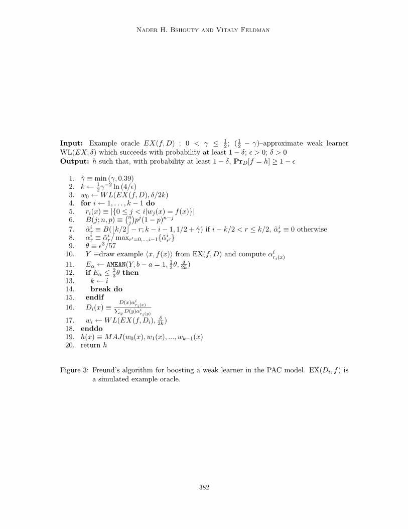
2 − γ)–approximatehypothesis with probability at least 1−δ′. Given these inputs, F1 steps sequentially throughk stages (k is given in Figure 3). At each stage i, 0 ≤ i ≤ k − 1 F1 generates distributionfunction Di, runs WL on simulated oracle EX(f,Di) and (with high probability) gets a(12 − γ)–approximate hypothesis wi. Simulation of the example oracle is done by filtering.
Probability of acceptance of the next example is estimated before the simulation (to Eα).If the probability is “too low” the algorithm does not produce any more weak hypotheses.Finally, F1 generates its hypothesis using majority function MAJ of all the wi it has received.
In Figure 3 we give the original implementation of Freund’s boosting algorithm F1.
Theorem 21 DNF is strongly learnable in the SQ–Dρ model.
Proof: The first and simple step towards the adaptation of Freund’s algorithm to SQ–D 14
is estimation of Eα using the procedure RV-SQ instead AMEAN (since we do not have accessto EX(f, D)). This is possible since the value of αi
ri(x) can be found using f(x) and previoushypotheses. Next, we show how to provide our weak learner with distribution Di. By the
definition, Di(x) ≡ D(x)αiri(x)P
y D(y)αiri(y)
. It is easy to see that given f(x) the value of D(x)αiri(x) can
be evaluated straightforwardly. On the other hand, the value of∑
y D(y)αiri(y) (independent
of x), which is the probability of accepting a sample from D, cannot be computed exactly.Instead, we can estimate this value. In fact, we already have the estimate: the value Eα usedfor termination condition (lines 12–14). The condition ensures that Eα ≥ 2
3θ (otherwise weterminate) and Eα is an estimate of
∑y D(y)αi
ri(y) within 1/3θ (line 11). Thus
1/2Eα ≤∑
y
D(y)αiri(y) ≤ 3/2Eα .
This means that if we define D′i(x) ≡ U(x)αi
ri(x)/Eα then we get that there is a constantci ∈ [1/2, 3/2] such that for all x, D′
i(x) = ciDi(x). Now consider the functional impactof supplying this approximate distribution rather than true distribution to WDNF 1
4. WDNF 1
4
uses its given distribution for exactly one purpose: to find the “large” Fourier coefficients offunction 2nDff . Since the Fourier transform is a linear operator (i.e., cg(a) = cg(a)) we canbe certain that 2nD′
if has a Fourier coefficient with absolute value of at least ci1
2s+1 ≥ 14s+2 .
Moreover, since the largest Fourier coefficient of 2nD′if corresponds to the largest Fourier
coefficient of 2nDif , the parity function corresponding to that coefficient (or its negation)
381
Nader H. Bshouty and Vitaly Feldman
Input: Example oracle EX(f,D) ; 0 < γ ≤ 12 ; (1
2 − γ)–approximate weak learnerWL(EX, δ) which succeeds with probability at least 1− δ; ε > 0; δ > 0Output: h such that, with probability at least 1− δ, PrD[f = h] ≥ 1− ε
1. γ ≡ min (γ, 0.39)2. k ← 1
2γ−2 ln (4/ε)3. w0 ← WL(EX(f,D), δ/2k)4. for i ← 1, . . . , k − 1 do5. ri(x) ≡ |0 ≤ j < i|wj(x) = f(x)|6. B(j; n, p) ≡ (
nj
)pj(1− p)n−j
7. αir ≡ B(bk/2c − r; k − i− 1, 1/2 + γ) if i− k/2 < r ≤ k/2, αi
r ≡ 0 otherwise8. αi
r ≡ αir/maxr′=0,...,i−1αi
r′9. θ ≡ ε3/57
10. Y ≡draw example 〈x, f(x)〉 from EX(f,D) and compute αiri(x)
11. Eα ← AMEAN(Y, b− a = 1, 13θ, δ
2k )12. if Eα ≤ 2
3θ then13. k ← i14. break do15. endif16. Di(x) ≡ D(x)αi
ri(x)Py D(y)αi
ri(y)
17. wi ← WL(EX(f,Di), δ2k )
18. enddo19. h(x) ≡ MAJ(w0(x), w1(x), ..., wk−1(x)20. return h
Figure 3: Freund’s algorithm for boosting a weak learner in the PAC model. EX(Di, f) isa simulated example oracle.
382

On Using Extended Statistical Queries to Avoid Membership Queries
(12 − 1
4s+2)–approximates target function with respect to Di. Thus by slightly modifying 7
WDNF 14
we can handle this problem. These modifications may increase the running time ofweak learner only by a small constant and thus do not affect our analysis.
Input: Access to STAT (f,D 14); s = DNF-size(f); ε > 0; δ > 0
Output: h such that, with probability at least 1− δ, PrU [f = h] ≥ 1− ε
1. γ ← 14s+4 ;
2. k ← 12γ−2 ln (4/ε)
3. w0 ←UWDNF 14(n, s, δ/k)
4. for i ← 1, . . . , k − 1 do5. ri(x) ≡ |0 ≤ j < i|wj(x) = f(x)|6. B(j; n, p) ≡ (
nj
)pj(1− p)n−j
7. αir ≡ B(bk/2c − r; k − i− 1, 1/2 + γ) if i− k/2 < r ≤ k/2, αi
r ≡ 0 otherwise8. αi
r ≡ αir/maxr′=0,...,i−1αi
r′9. θ ← ε3/57
10. Eα ←RV-SQ(STAT(f, U), αiri(x), 1, θ/3)
11. if Eα ≤ 23θ then
12. k ← i
13. break do14. endif15. D′
i(x) ≡ U(x)αiri(x)/Eα
16. wi ←WDNF 14(n, s,D′
i, 3/(2θ), δ/k)
17. enddo18. h(x) ≡ MAJ(w0(x), w1(x), ..., wk−1(x))19. return h
Figure 4: Learning DNF in the SQ–D 14
model
In Figure 4 we give a straightforward implementation of the discussed adaptation.Our last concern is the complexity of this algorithm. The total number of phases
executed will be O(s2 log ε−1). Clearly the “heaviest” part of each phase is the execu-tion of the weak learner. By Theorem 20, the running time of each call to WDNF 1
4is
O(ns12ε−24 log (1/δ)). Thus the total running time of the algorithm is O(ns14ε−24 log (1/δ)).The tolerance of queries is Ω(s−4ε12). The complexity of query functions is as complexityof evaluation of αi
ri(x) plus O(n). All the O(k2) = O(s4) possible values of αiri(x) can be
evaluated in advance, that is complexity of query functions will be O(n). ¤
The adaptation of boosting algorithm that we obtained is not suitable for boosting weaklearners which will fail when supplied with distributions D′
i as above instead of Di. Except
7. Lower bound θ has to be modified to 14s+2
.
383

Nader H. Bshouty and Vitaly Feldman
for this limitation we, in fact, described the general way to boost weak learners in the SQ–Dmodel.
Recently, two new boosting algorithms have appeared that use only distributions thatare polynomially close to the uniform. The first one is by Klivans and Servedio [KS99]and the second one is by Bshouty and Gavinsky [BG01]. Distributions produced by theseboosting algorithms are optimally “flat”, that is, the L∞ norm of distributions they produceis O(ε)2−n. They also require the same order of phases as F1. Both algorithms are morecomplicated than F1, but nevertheless can be adapted to SQ–D in a very similar way.These algorithms were used to improve the running time of Jackson’s original algorithmand can be substituted for F1 in our algorithm as well. This would significantly decreasethe dependence on ε. In particular, L∞(Di) = O(ε−1) and k = O(γ−2 log (1/ε)) gives therunning time of O(ns14ε−8 log (1/δ)) and tolerance becomes lower-bounded by Ω(s−4ε4).
4. Learning with Attribute Noise in Membership Queries
We now turn our attention to another type of noise in membership queries: the noise thatcorrupts the attributes of a sample point. That is, as an answer to a membership queryat point x the learner gets the value of f(x′), where x′ might differ from x. This type ofnoise was previously considered as appearing in the example oracle EX(f, D), that is thelearner gets random labelled samples (x, f(x′)) [SV88; GS95; BJT99]. We define the noisemodel formally and then focus our attention on the product attribute noise with knownnoise rate (which is the most commonly referred type of attribute noise). We prove thatmembership queries corrupted by such a noise are weaker than extended statistical queriesdiscussed in the previous chapter. Nevertheless, the Bounded Sieve can be implemented inthis model. This implies that DT is learnable and DNF is weakly learnable in this “weak”model. We prove that these learning results can also be achieved for the uniform productattribute noise of unknown rate.
4.1 The Noise Model and Its Properties
The attribute noise is usually described as returning the value f(x⊕ b) where b is sampledrandomly with respect to some noise distribution D′. The simplest and the most wellstudied noise distribution is the product distribution, i.e., independence of all the attributesis assumed.8 If every attribute is changed with the same probability the noise is calleduniform. The resulting model represents the situation in which the learner cannot ask themembership query in the desired point since the attributes it supplies change their staterandomly and independently in the process of the query. Examples of situations of thiskind are:
• sending the point x to the oracle via a faulty communication channel9
• “material” representing the attributes is unstable.
8. This assumption certainly agrees with assumptions of learning with respect to the uniform.9. For this case the attribute noise is uniform and random classification noise has to be added if the answer
is also sent via a faulty channel.
384
On Using Extended Statistical Queries to Avoid Membership Queries
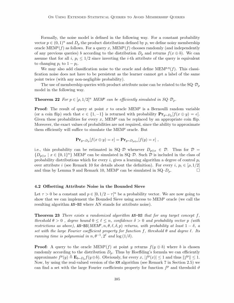
Formally, the noise model is defined in the following way. For a constant probabilityvector p ∈ (0, 1)n and Dp the product distribution defined by p, we define noisy membershiporacle MEMp(f) as follows. For a query x, MEMp(f) chooses randomly (and independentlyof any previous queries) b according to the distribution Dp and returns f(x ⊕ b). We canassume that for all i, pi ≤ 1/2 since inverting the i-th attribute of the query is equivalentto changing pi to 1− pi.
We may also add classification noise to the oracle and define MEMp,η(f). This classi-fication noise does not have to be persistent as the learner cannot get a label of the samepoint twice (with any non-negligible probability).
The use of membership queries with product attribute noise can be related to the SQ–Dρ
model in the following way.
Theorem 22 For p ∈ [ρ, 1/2]n MEMp can be efficiently simulated in SQ–Dρ.
Proof: The result of query at point x to oracle MEMp is a Bernoulli random variable(or a coin flip) such that e ∈ 1,−1 is returned with probability Pry∼Dp [f(x ⊕ y) = e].Given these probabilities for every x, MEMp can be replaced by an appropriate coin flip.Moreover, the exact values of probabilities are not required, since the ability to approximatethem efficiently will suffice to simulate the MEMp oracle. But
Pry∼Dp [f(x⊕ y) = e] = Pry∼Dp⊕x [f(y) = e] ,
i.e., this probability can be estimated in SQ–D whenever Dp⊕x ∈ D. Thus for D =Dp⊕x | x ∈ 0, 1n MEMp can be simulated in SQ–D. Such D is included in the class ofprobability distributions which for every i, gives a learning algorithm a degree of control pi
over attribute i (see Remark 10 for details about the definition). For every i, pi ∈ [ρ, 1/2]and thus by Lemma 9 and Remark 10, MEMp can be simulated in SQ–Dρ. ¤
4.2 Offsetting Attribute Noise in the Bounded Sieve
Let τ > 0 be a constant and p ∈ [0, 1/2− τ ]n be a probability vector. We are now going toshow that we can implement the Bounded Sieve using access to MEMp oracle (we call theresulting algorithm AN-BS where AN stands for attribute noise).
Theorem 23 There exists a randomized algorithm AN-BS that for any target concept f ,threshold θ > 0 , degree bound 0 ≤ ` ≤ n, confidence δ > 0 and probability vector p (withrestrictions as above), AN-BS(MEMp, n, θ, `, δ, p) returns, with probability at least 1 − δ, aset with the large Fourier coefficient property for function f , threshold θ and degree `. Itsrunning time is polynomial in n, θ−1, 2` and log (1/δ).
Proof: A query to the oracle MEMp(f) at point y returns f(y ⊕ b) where b is chosenrandomly according to the distribution Dp. Thus by Hoeffding’s formula we can efficientlyapproximate fp(y) , Eb∼Dpf(y⊕ b). Obviously, for every x, |fp(x)| ≤ 1 and thus ‖fp‖ ≤ 1.Now, by using the real-valued version of the KM algorithm (see Remark 7 in Section 2.5) wecan find a set with the large Fourier coefficients property for function fp and threshold ϑ
385

Nader H. Bshouty and Vitaly Feldman
in time polynomial in n, ϑ−1 and log (1/δ). But
fp(y) = Eb∼Dp [f(y⊕b)] =∑
a∈0,1n
f(a)Eb∼Dp [χa(y⊕b)] =∑
a∈0,1n
(f(a)Eb∼Dp [χa(b)]
)χa(y),
i.e., we have that for all a, fp(a) = f(a)Eb∼Dpχa(b). We can easily calculate the valueca , Eb∼Dpχa(b) =
∏ai=1(1− 2pi). By the properties of p, |ca| ≥ (2τ)w(a). Thus if we run
the above algorithm for the threshold ϑ = (2τ)`θ we will get the set S′ that includes a setwith the large Fourier coefficient property for the function f and threshold θ. Size of S′ isbounded by (2τ)−2`θ−2. In order to estimate the values of the coefficient f(a) with accuracyσ we estimate the coefficient fp(a) with accuracy σca ≥ (2τ)`σ and return c−1
a fp(a). Thuswe can refine the set S′ and return a set with the large Fourier coefficient property for thefunction f , threshold θ and degree `. All the parts of the described algorithm run in timepolynomial in n, (2τ)−`θ−1 and log (1/δ), that is, for a constant τ the time is polynomial inn, θ−1, 2`, and log (1/δ) ¤
Remark 24 It is easy to note that knowing the noise rates exactly is not necessary. Thatis, the result will hold when the learning algorithm is supplied with “good” estimates of thenoise rates. Particularly, estimates within inverse of a polynomial (in learning parameters)will suffice.
Remark 25 When using MEMp,η(f) oracle instead of MEMp(f) in the above algorithm wecan immediately offset the classification noise by using the fact: fp,η(y) = (1 − 2η)fp(y),where fp,η(y) is the expectation of the query in point y to the oracle MEMp,η(f). This willrequire increasing the accuracy of the estimation by 1
1−2η and make the running time of thealgorithm polynomially dependent on 1
1−2η .
By sole use of AN-BS we can efficiently learn DT and weakly learn DNF as described inTheorems 16 and 19.
4.3 Coping with Attribute Noise of Unknown Rate
As was shown by Goldman and Sloan [GS95], coping with attribute noise becomes muchmore difficult when the noise rates are unknown.10 The reason for this is that the usualway of handling the unknown noise rate—choosing the hypotheses with the minimum dis-agreement on samples—does not work for this type of noise. Nevertheless, several simpleclasses (e.g., k−DNF and monomials) are learnable when the attribute noise is uniform[GS95; DG95]. The following two theorems show that our learnability results hold in thissetting as well.
Theorem 26 DT is learnable by membership queries with uniform attribute noise of fixedunknown rate ν < 1/2.
10. In fact, no PAC learning algorithm exists that can tolerate a noise rate higher than 2ε, where ε is therequired accuracy parameter.
386

On Using Extended Statistical Queries to Avoid Membership Queries
Sketch of proof: Learning algorithm has access to MEMp oracle for p = [ν]n. For theease of presentation let us assume that all estimations we do by sampling produce the exactresult. In particular, our AN-BS algorithm returns all the vectors with Fourier coefficientslarger than the bound that was given to it(and only them) and we can estimate exactlycoefficients of the function fp defined in the proof of Theorem 23. For positive ν ′ < 1/2 welook at the execution of AN-BS for learning DT supplied with noise rate ν ′ (equal for all theattributes) instead of the actual noise rate, i.e.,
AN-BS(δ,MEMp, n,ε
8s, log
8s
ε, [ν ′]n)
We then find all the Fourier coefficients for returned vectors and offset the effect of noiseby multiplying every coefficient fp(a) by (1− 2ν ′)−w(a) (as if ν ′ is a correct noise rate). Wedenote the function defined by coefficients we have found by fp
ν′ (with the assumptions wemade this function is well-defined). If ν ′ = ν then the algorithm we have just described willfind all the required vectors and calculate their Fourier coefficients correctly. Thus, as followsfrom Lemma 15, 1− ε < ‖fp
ν ‖2 ≤ 1. It is easy to note that the larger the supplied noise rateν ′ is, the more vectors the execution of AN-BS returns (since the threshold gets lower) andthe larger is the value by which we multiply every Fourier coefficient of fp that was foundby AN-BS. That is, for every a ∈ 0, 1n, |fp
ν′(a)| and ‖fpν′‖2 are monotonous in ν ′. Thus by
using a binary search we can efficiently find a value ν ′ for which 1− ε ≤ ‖fpν′‖2 ≤ 1 + ε (∗)
(the search will be efficient since values which are “close” to ν will satisfy this criterion).Denote the value we have found by ν1. As we have noted, for every vector a, |fp
ν′(a)| ismonotonous in ν ′ thus the criterion (∗) that ν1 satisfies ensures that
∣∣‖fpν ‖2 − ‖fp
ν′‖2∣∣ =
∣∣∣∣∣∑
a
(fp
ν2(a)− fp
ν′2(a)
)∣∣∣∣∣ ≤ 2ε (8)
On the other hand, as it was shown in the proof of Theorem 16, sign(fpν ) ε–approximates f
and therefore ∑a
(fp
ν (a)− f(a))2≤ ε (9)
By combining equations 8 and 9 we can easily obtain that
∑a
(fp
ν1(a)− f(a))2≤ 3ε (10)
That is, sign(fpν1) 3ε–approximates f . ¤
Remark 27 Without the “exactness” assumption we made in this proof we will need toimprove the tolerance of all the queries so that the overall error in computation of fp
ν′ besmaller than ε/8 (and substitute ε/4 for ε in other bounds).
Theorem 28 DNF is weakly learnable by membership queries with uniform attribute noiseof fixed unknown rate ν < 1/2.
387
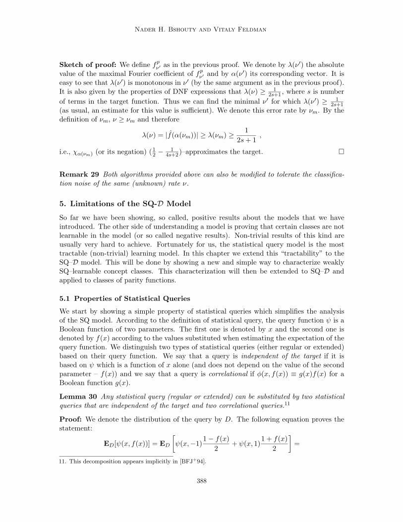
Nader H. Bshouty and Vitaly Feldman
Sketch of proof: We define fpν′ as in the previous proof. We denote by λ(ν ′) the absolute
value of the maximal Fourier coefficient of fpν′ and by α(ν ′) its corresponding vector. It is
easy to see that λ(ν ′) is monotonous in ν ′ (by the same argument as in the previous proof).It is also given by the properties of DNF expressions that λ(ν) ≥ 1
2s+1 , where s is numberof terms in the target function. Thus we can find the minimal ν ′ for which λ(ν ′) ≥ 1
2s+1(as usual, an estimate for this value is sufficient). We denote this error rate by νm. By thedefinition of νm, ν ≥ νm and therefore
λ(ν) = |f(α(νm))| ≥ λ(νm) ≥ 12s + 1
,
i.e., χα(νm) (or its negation) (12 − 1
4s+2)–approximates the target. ¤
Remark 29 Both algorithms provided above can also be modified to tolerate the classifica-tion noise of the same (unknown) rate ν.
5. Limitations of the SQ-D Model
So far we have been showing, so called, positive results about the models that we haveintroduced. The other side of understanding a model is proving that certain classes are notlearnable in the model (or so called negative results). Non-trivial results of this kind areusually very hard to achieve. Fortunately for us, the statistical query model is the mosttractable (non-trivial) learning model. In this chapter we extend this “tractability” to theSQ–D model. This will be done by showing a new and simple way to characterize weaklySQ–learnable concept classes. This characterization will then be extended to SQ–D andapplied to classes of parity functions.
5.1 Properties of Statistical Queries
We start by showing a simple property of statistical queries which simplifies the analysisof the SQ model. According to the definition of statistical query, the query function ψ is aBoolean function of two parameters. The first one is denoted by x and the second one isdenoted by f(x) according to the values substituted when estimating the expectation of thequery function. We distinguish two types of statistical queries (either regular or extended)based on their query function. We say that a query is independent of the target if it isbased on ψ which is a function of x alone (and does not depend on the value of the secondparameter – f(x)) and we say that a query is correlational if φ(x, f(x)) ≡ g(x)f(x) for aBoolean function g(x).
Lemma 30 Any statistical query (regular or extended) can be substituted by two statisticalqueries that are independent of the target and two correlational queries.11
Proof: We denote the distribution of the query by D. The following equation proves thestatement:
ED[ψ(x, f(x))] = ED
[ψ(x,−1)
1− f(x)2
+ ψ(x, 1)1 + f(x)
2
]=
11. This decomposition appears implicitly in [BFJ+94].
388

On Using Extended Statistical Queries to Avoid Membership Queries
12ED[ψ(x, 1)f(x)]− 1
2ED[ψ(x,−1)f(x)] +
12ED[ψ(x, 1)] +
12ED[ψ(x,−1)] .
¤
A query that is independent of the target is estimation of the expectation of randomvariable which is independent of f and therefore such a query can be substituted by a callto procedure AMEAN (we assume that the learning algorithm is able to sample randomly withrespect to the distribution of the query). Thus we may assume that learning algorithms inthe statistical query based models use only the correlational statistical queries.
5.2 The Characterization
We are now going to present the characterization of classes weakly learnable in statisticalquery based models. Let F be the concept class and A be an algorithm that weakly learnsF in the SQ model (and uses only correlational queries). The characterization is basedon the following observation: for every (but, probably, one) function in F there exists acorrelational query for which A gets a reply which differs “noticeably” from 0. This is truebecause there could not exist two different functions in F for which the results of all thequeries are “almost” equal. For every f ∈ F denote by gf the function for which |ED[fgf ]|differs “noticeably” from 0, that is, gf (or its negation) weakly approximates f . This meansthat the set of queries of A weakly “approximates” all (but, probably, one) functions inF . This argument is formalized in the following way. Let V and W be sets of Booleanfunctions. We say that W ε–approximates V with respect to distribution D if for everyf ∈ V there exists g ∈ W such that g ε–approximates f with respect to distribution D. Fora concept class F denote by Fs the set of all the functions in F of size s.
Theorem 31 Let F be a concept class weakly SQ–learnable with respect to D, particu-larly, there exists an algorithm A that for every f ∈ Fs, uses at most p(n, s) queries oftolerance lower-bounded by 1
r(n,s) to produce (12 − 1
q(n,s))–approximation to f . Let r′(n, s) ,max2r(n, s), q(n, s). There exists a collection of sets Wi∞i=1 such that |Ws| ≤ p(n, s)+1and Ws (1
2 − 1r′(n,s))–approximates Fs with respect to D.
Proof: According to the above discussion, we may assume that A uses only correlationalqueries. We build the set Ws as follows. We simulate algorithm A(n, s) and for every query(fgi, ρ) we add gi to Ws and return the value 0 as a result of the query. We continuethe simulation till it violates any of the complexity bounds of A or A stops and returnsfinal hypothesis h. In the later case we also add h to Ws. First, by the definition of Ws,|Ws| ≤ p(n, s) + 1. Now, assume that Ws does not (1
2 − 1r′(n,s))–approximate Fs, i.e., there
exists f ∈ Fs such that for every g ∈ Ws, |ED[fg]| < 2r′(n,s) . This means that in our
simulation for building Ws, zeros that we gave as answers are valid answers to the queries.Therefore, by the definition of A, it returns hypothesis h that (1
2 − 1q(n,s))–approximates f ,
that is, h ∈ Ws. This contradicts the assumption that |ED[fh]| < 2r′(n,s) ≤ 2
q(n,s) . ¤
In the above proof we assumed that A is a deterministic algorithm. On the otherhand, the proof does not rely on the uniformity of the algorithm A (our only restrictionis the polynomial number of queries). As is well known, any randomized algorithm can be
389
Nader H. Bshouty and Vitaly Feldman
transformed into non-uniform (deterministic) algorithm (in the context of languages thisresult is referred as BPP ⊂ P/poly). Therefore, Theorem 31 is also true for classes weaklylearnable by randomized algorithms.
This characterization can be easily extended to SQ–D in the following way. Every query(fg, ρ, D′) to STAT(f,D) has its own distribution D′ ∈ D. Thus the fact that results of aquery differ “noticeably” from 0 means that f is weakly approximated with respect to somedistribution from D. Distinct queries may use distinct distributions from D and thereforealong with every function in the approximating collection of sets we need to record thedistribution with respect to which function in F is approximated. Formally, we say that aset W ⊆ −1, 1X ×D ε–approximates the set V of Boolean functions with respect to D iffor every f ∈ V there exists a pair (g, D′) ∈ W such that g ε–approximates f with respectto D′. Theorem 31 is generalized to SQ–D as follows.
Theorem 32 Let F be a class learnable in SQ–D. For p and r′ defined as in Theorem 31there exists a collection of sets Wi∞i=1 such that Ws ⊆ −1, 1X × D, |Ws| ≤ p(n, s) + 1and Ws (1
2 − 1r′(n,s))–approximates Fs with respect to D.
5.3 Applications
Although the characterization we gave for the SQ model is not equivalent to characterizationby SQ–DIM [BFJ+94] (see Section 1.1 for more details) it is applied in a very similar way.To demonstrate this we give a new proof for the main result obtained using the SQ–DIMcharacterization.
Theorem 33 Any concept class containing superpolynomial number of parity functions isnot weakly SQ–learnable with respect to the uniform distribution.
Proof: Since the size of representation of any parity function is bounded by a fixed polyno-mial (e.g., c0n) by Theorem 31 (with Remark 1) we have that there exist polynomials r(n)and p(n) such that F has a (1
2 − 1r(n))–approximating set W of size bounded by p(n). For
any g ∈ W approximating a parity function χa means that |E[g(x)χa]| = |g(a)| ≥ 2/r(n).But from Parseval’s identity we know that
∑a∈0,1n g2(a) = 1. This means that at most
r2(n)/4 Fourier coefficients of g could be greater than 2/r(n), i.e., every g ∈ W could becorrelated with at most r2(n)/4 different parity functions. On the other hand, |W | ≤ p(n),that is, W can approximate at most p(n)r2(n)/4 parity functions. Thus, any F containinga superpolynomial number of parity functions is not weakly SQ–learnable with respect tothe uniform distribution. ¤
Our characterization of SQ–D learnable classes can be used to show the limitations ofthe SQ–Dρ model. BSρ can be straightforwardly used to learn the class of all parity functioncontaining at most O(log n) variables (with respect to U). On the other hand, we will showthat the class of all the parity functions containing at most c(n) log n variables for unboundedc(n) cannot be learned in SQ–Dρ. For this purpose we denote by Ak = 0, 1k[0]n−k, andlet PARk denote the class of all parity functions for vectors in Ak, i.e., all parity functionsbased on the first k variables. In fact, we give somewhat stronger result.
Theorem 34 PARk is not weakly learnable in SQ–Dρ for k(n) = ω(log n).
390

On Using Extended Statistical Queries to Avoid Membership Queries
Proof: Assume that the theorem is not true. By Theorem 32 (with Remark 1) there existpolynomials p(n) and r(n) and set of pairs W = (g1, D1), (g2, D2), . . . , (gm, Dm) such that|W | = m ≤ p(n) and for every χa ∈ PARk there exists (gi, Di) ∈ W , where Di ∈ Dρ, suchthat EDi [giχa] ≥ 1/r(n). This means that
∑1≤i≤m E2
Di[giχa] ≥ 1/r2(n). Thus
∑
a∈Ak
∑
1≤i≤m
E2Di
[giχa] ≥ |Ak|/r2(n)
This means that there exists i such that∑
a∈Ak
E2Di
[giχa] ≥ |Ak|/(|W |r2(n)) ≥ |Ak|/(p(n)r2(n)).
Or, if we denote by Uk a uniform distribution over Ak, then we get that
I , Ea∼Uk
[E2
Di[giχa]
] ≥ 1/(p(n)r2(n)). (11)
On the other hand,
I = Ea∼Uk
[E2
Di[giχa]
]= Ea∼Uk [Ex∼Di [Ey∼Di [gi(x)χa(x)gi(y)χa(y)]]]
= Ex∼Di [Ey∼Di [gi(x)gi(y)Ea∼Uk [χa(x⊕ y)]]] . (12)
But
λ(z) , Ea∼Uk [χa(z)] = Ea∼Uk [χz[1,k](a[1,k])] =
0 z[1,k] 6= [0]k
1 z[1,k] = [0]k
Since λ(x⊕ y) is non-negative and |gi(x)gi(y)| = 1, equation (12) yields that
I ≤ Ex∼Di [Ey∼Di [λ(x⊕ y)]] = Ex∼Di [Pry∼Di [λ(x⊕ y) = 1]]
= Ex∼Di [Pry∼Di [y[1,k] = x[1,k]]] ≤ Ex∼Di [(1− ρ)k] ≤ (1− ρ)k . (13)
For k = ω(log n), (1 − ρ)k cannot be lower-bounded by inverse of a polynomial and thusequation (11) contradicts equation (13). ¤
The last theorem may also be used to prove that the set of concept classes learnablein the PAC model with classification noise of constant rate is not contained in the set ofconcept classes weakly learnable in SQ–D 1
4. This result can be obtained by combining our
result with the following theorem for k = log n log log n [BKW00, Theorem 2].
Theorem 35 PARk for noise rate η equal to any constant less than 12 , can be learned with
respect to the uniform distribution using number of samples and total computation time2O(k/ log k).
Another interesting application of our characterization is to demonstrate that PAR,the class of all parity functions, possesses some inherent hardness for any statistics basedlearning. For this purpose we give the following definition. We say that a distribution classD is biased if there exist a polynomial p(n) such that L∞(D) ≥ 1
p(n) . We may notice thatif a distribution class D is biased then a non-uniform learning algorithm may get the valueof the target function at the “biased” point. Use of attributes of specific point togetherwith its label contradicts the idea of statistical learning and, on the other hand, is the mainelement of all the known algorithms for learning of parity functions.
391

Nader H. Bshouty and Vitaly Feldman
Theorem 36 Let D be a class of distributions. If D is not biased then for every D ∈ D,PAR is not weakly learnable in the SQ–D model with respect to D.
Proof: By assuming that PAR is weakly learnable in SQ–D with respect to some distribu-tion D ∈ D and then proceeding as in the proof of the previous theorem we get that thereexists set W and (gi, Di) ∈ W (Di ∈ D) such that
Ea∼U
[E2
Di[giχa]
] ≥ 1/(p(n)r2(n)).
On the other hand,
Ea∼U
[E2
Di[giχa]
]= Ea∼U [Ex∼Di [Ey∼Di [gi(x)χa(x)gi(y)χa(y)]]]
= Ex∼Di [Ey∼Di [gi(x)gi(y)Ea∼U [χa(x⊕ y)]]] (14)
By the properties of parity functions, if x 6= y then Ea∼U [χa(x⊕ y)] = Ea∼U [χx⊕y(a)] = 0.Otherwise, Ea∼U [χa(0n)] = 1. So the expression we are evaluating is equal to
Ex∼Di [Di(x)g2i (x)] = Ex∼Di [Di(x)]
Thus we got that Ex∼Di [Di(x)] ≥ 1/(p(n)r2(n)), in particular there exists x such thatDi(x) ≥ 1/(p(n)r2(n)), that is, D is biased. This contradiction finishes the proof. ¤
6. Conclusions and Open Problems
In this work we have shown that DNF is learnable in an extension of the PAC model (PAC-Dρ) that seems to be weaker than the use of membership queries. While it seems to bevery difficult to say anything about the exact strength of the PAC-Dρ model, we can showthat the statistical query analogue of PAC-Dρ (SQ–Dρ) is sufficient for our DNF learningalgorithm. This fact combined with characterization of SQ–Dρ learnable classes was used toshow that, in terms of learning parity functions, SQ–Dρ has just enough power to be able tolearn parity functions that can be expressed as polynomial-size DNF expressions. Anotheruseful property of the SQ–Dρ model used is that it can be simulated using membershipqueries with persistent classification noise.
We have introduced an extension of attribute noise to membership queries. It turns outthat the use of membership queries with product attribute noise is interestingly related tothe SQ–Dρ model. We have shown that decision trees are learnable and DNF expressionsare weakly learnable by membership queries with product attribute noise.
The introduction of new model between PACU and PACU+MQ poses interesting andapparently difficult questions about the relation between the strengths of these models.Another interesting question of similar nature is whether there exists a class learnable in SQ–Dρ and not learnable by membership queries with product attribute noise, and particularly(in case the answer is positive) whether DNF is such a class. As we have proved, the powerof SQ–Dρ does not decrease when we decrease ρ. But it remains unclear to us whether thepower is strictly increasing or the models are equally strong (for a constant 0 < ρ < 1/2).
392
On Using Extended Statistical Queries to Avoid Membership Queries
Acknowledgments
This research was supported by the fund for the promotion of research at the Technion.Part of research was done at the University of Calgary, Calgary, Alberta, Canada.
We would like to thank Dmitry Gavinsky, Jeff Jackson and Eyal Kushilevitz for use-ful discussions about this research, and to anonymous referees of COLT/EuroCOLT 2001conference and Journal of Machine Learning Research for their careful reading, corrections,and insightful comments on this work.
References
[AD93] Javed Aslam, Scott Decatur. General Bounds on Statistical Query Learning andPAC Learning with Noise via Hypothesis Boosting. In Proceedings of 34-th AnnualSymposium on Foundations of Computer Science, pp. 282–291, 1993.
[AL88] Dana Angluin, Philip Laird. Learning From Noisy Examples. In Machine Learning,2(4) pp.343–370, 1988.
[AK91] Dana Angluin, Michael Kharitonov. When Won’t Membership Queries Help? InProceedings of the 23-rd Annual ACM Symposium on Theory of Computing, 1991, pp.454–454.
[Bs93] Nader Bshouty. Exact Learning via the Monotone Theory. In Proceedings of 34-thAnnual Symposium on Foundations of Computer Science, pp. 302–311, 1993.
[BFJ+94] Avrim Blum, Merrick Furst, Jeffrey Jackson, Michael Kearns, Yishay Mansour,Steven Rudich. Weakly Learning DNF and Characterizing Statistical Query LearningUsing Fourier Analysis. In Proceedings of the 26-th Annual ACM Symposium on theTheory of Computing, pp. 253–262, 1994.
[BF01] Nader Bshouty, Vitaly Feldman. On Using Extended Statistical Queries toAvoid Membership Queries. In Proceedings of the 14-th Annual Conference onCOLT/EuroCOLT, pp. 529–545, 2001.
[BG01] Nader Bshouty, Dmitry Gavinsky. On Boosting With Optimal Poly-Bounded Dis-tributions. In Proceedings of the 14-th Annual Conference on COLT/EuroCOLT, pp.490–506, 2001.
[BJT99] Nader Bshouty, Jeffrey Jackson, Christino Tamon. Uniform-Distribution AttributeNoise Learnability. In Proceedings of the 12-th Annual Conference on COLT, pp. 75–80,1999.
[BKW00] Avrim Blum, Adam Kalai, Hal Wasserman. Noise-Tolerant Learning, the ParityProblem and the Statistical Query Model. In Proceedings of the 32-th Annual ACMSymposium on Theory of Computing, pp. 435–440, 2000.
[DG95] Scott Decatur, Rosario Gennaro. In Proceedings of the Eighth Annual ACM Work-shop on Computational Learning Theory, pp.353–360, 1995.
393

Nader H. Bshouty and Vitaly Feldman
[Fr90] Yoav Freund. Boosting a Weak Learning Algorithm by Majority. In Proceedings ofthe Third Annual Workshop on COLT, pp. 202–216, 1990.
[FS94] Yoav Freund, Robert Schapire. A Decision-theoretic Generalization of On-lineLearning and an Application to Boosting. In Proceedings of the Second Annual Eu-ropean Conference on Computational Learning Theory, 1994.
[GKS94] Sally Goldman, Michael Kearns, Robert Shapire. Exact Identification of CircuitsUsing Fixed Points of Amplification Functions, In SIAM Journal on Computing, 22(1993), pp. 705–726.
[GL89] Oded Goldreich, Leonid A. Levin. A Hard-Core Predicate for all One-Way Func-tions. In Proceedings of the Twenty First Annual ACM Symposium on Theory of Com-puting, pp. 25–32, 1989.
[GS95] Sally Goldman, Robert Sloan. Can PAC Learning Algorithms Tolerate RandomAttribute Noise? In Algorithmica, 14(1) pp. 70–84, 1995.
[Ja94] Jeffrey Jackson. An Efficient Membership-Query Algorithm for Learning DNF withRespect to the Uniform Distribution. In Proceedings of the 35th Annual Symposion onFoundations of Computer Science, pp. 42–53, 1994.
[Ja97] Jeffrey Jackson. An Efficient Membership-Query Algorithm for Learning DNF withRespect to the Uniform Distribution. In Journal of Computer and System Sciences,55(3), 1997
[JSS97] Jeffrey Jackson, Eli Shamir, Clara Shwartzman. Learning with Queries Corruptedby Classification Noise. In Proceedings of Fifth Israel Symposium on Theory of Com-puting and Systems, pp. 45–53, 1997.
[Kea93] Michael Kearns. Efficient Noise-Tolerant Learning from Statistical Queries. In Pro-ceedings of the Forth Annual Workshop on COLT, pp. 392–401, 1993.
[KM91] Eyal Kushilevitz, Yishay Mansour. Learning Decision Trees Using the Fourier Spec-trum. In Proceedings of the 23-rd Annual Symposium on Theory of Computing, pages455–464.
[KS99] Adam Klivans, Rocco Servedio. Boosting and Hard-Core Sets. In Proceedings of40-th Annual Symposium on Foundations of Computer Science, pp. 624–633, 1999.
[KSS92] Michael Kearns, Robert Shapire, Linda Sellie. Toward Efficient Agnostic Learning.In Proceedings of the Fifth Annual Workshop on COLT, pp. 341–352, 1992.
[Lai88] Phillip D. Laird. Learning From Good and Bad Data. Kluwer Academic Publishers,Boston, 1988.
[LMN89] Nathan Linial, Yishay Mansour, Noam Nisan. Constant Depth Circuits, FourierTransform, and Learnability. In Proceedings of the 31-st Symposium on the Foundationsof Computer Science, pp. 574–579, 1989.
394
On Using Extended Statistical Queries to Avoid Membership Queries
[Man94] Yishay Mansour. Learning Boolean Functions via the Fourier Transform. In The-oretical Advances in Neural Computation and Learning, (V.P. Roychodhury and K-Y.Siu and A. Orlitsky, ed.), 391–424, 1994.
[ShSh95] Eli Shamir, Clara Shwartzman. Learning by Extended Statistical Queries and ItsRelation to PAC Learning. In Proceedings of Second European Conference, EuroCOLT’95, pp. 357–366, 1995.
[Sch90] Robert Shapire. The Strength of Weak Learnability. In Machine Learning, 5, pp.197–227, 1990.
[Sl88] Robert Sloan. Types of Noise in Data for Concept Learning. In Proceedings of the1988 Workshop on Computational Learning Theory, pp. 91–96, MIT, ACM Press, 1988.
[SV88] George Shakelford, Dennis Volper. Learning k−DNF with Noise in the Attributes.In Proceedings of the 1988 Workshop on COLT, pp. 97–103, 1988.
[V84] Leslie Valiant. A Theory of the Learnable. In Commmunications of the ACM, 27(11)pp. 1134–1142, 1984.
395


![FLOW TEMP. CONTROLLER [MASTER] (Cased) PAC-IF051B-E PAC-IF052B-E FLOW TEMP. CONTROLLER ... · 2013. 2. 12. · PAC-IF051B-E PAC-IF052B-E FLOW TEMP. CONTROLLER [SLAVE] (Cased) PAC-SIF051B-E](https://img.pdfslide.us/doc/110x75/612d85651ecc515869423db7/flow-temp-controller-master-cased-pac-if051b-e-pac-if052b-e-flow-temp-controller.jpg)