On Turing complete T7 and MISC F-4

program fitness landscapes

W. B. Langdon and R. PoliDepartment of Computer Science, University of Essex, UK

Technical Report CSM-445

19 December 2005

Abstract

We use the minimal instruction set F-4 computer to define a minimal Turing completeT7 computer suitable for genetic programming (GP) and amenable to theoretical analy-sis. Experimental runs and mathematical analysis of the T7, show the fraction of haltingprograms is drops to zero as bigger programs are run.

1 Introduction

Recent work on strengthening the theoretical underpinnings of genetic programming (GP) hasconsidered how GP searches its fitness landscape [Langdon and Poli, 2002; McPhee and Poli,2001; McPhee et al., 2001; McPhee and Poli, 2002; Rosca, 2003; Sastry et al., 2003; Greene, 2004;Poli et al., 2004; Mitavskiy and Rowe, 2005; Daida et al., 2005]. Results gained on the space ofall possible programs are applicable to both GP and other search based automatic programmingtechniques. We have proved convergence results for the two most important forms of GP, i.e.trees (without side effects) and linear GP [Langdon and Poli, 2002; Langdon, 2002a; Langdon,2002b; Langdon, 2003b; Langdon, 2003a]. As remarked more than ten years ago [Teller, 1994],it is still true that few researchers allow their GP’s to include iteration or recursion. Indeedthere are only about 50 papers (out of 4631) where loops or recursion have been included inGP. These are listed in Appendix B. Without some form of looping and memory there arealgorithms which cannot be represented and so GP stands no chance of evolving them.

We extend our results to Turing complete linear GP machine code programs. We analysethe formation of the first loop in the programs and whether programs ever leave that loop.Mathematical analysis is followed up by simulations on a demonstration computer. In particularwe study how the frequency of different types of loops varies with program size. In the processwe have executed programs of up to 16 777 215 instructions. These are perhaps the largestprograms ever (deliberately) executed as part of a GP experiment. (beating the previous largestof 1 000 000 [Langdon, 2000]). Results confirm theory and show that, the fraction of programsthat produce usable results, i.e. that halt, is vanishingly small, confirming the popular viewthat machine code programming is hard.

The next two sections describe the T7 computer (see Figure 1) and simulations run on it,whilst Sections 4 and 5 present theoretical models and compare them with measurement ofhalting and non-halting programs. The implications of these results are discussed in Section 6before we conclude (Section 7).

1Dagstuhl Seminar Proceedings 06061Theory of Evolutionary Algorithmshttp://drops.dagstuhl.de/opus/volltexte/2006/595

brought to you by COREView metadata, citation and similar papers at core.ac.uk

provided by Dagstuhl Research Online Publication Server

9

10

11

12

13

14

CPU

8

0

1

2

3

4

5

6

7Start

Program counter

0

8

16

24

32

40

48

56

64

72

80

88

ADD

Overflow flag

ProgramMemory (12 bytes=96bits)

BVS 3

STi 26, 21

LDi 79, 14

CPY 88, 55

JMP 53

ADD 72,27 45

CPY 78, 2

LDi 3, 9

CPY 0, 20

BVS 6

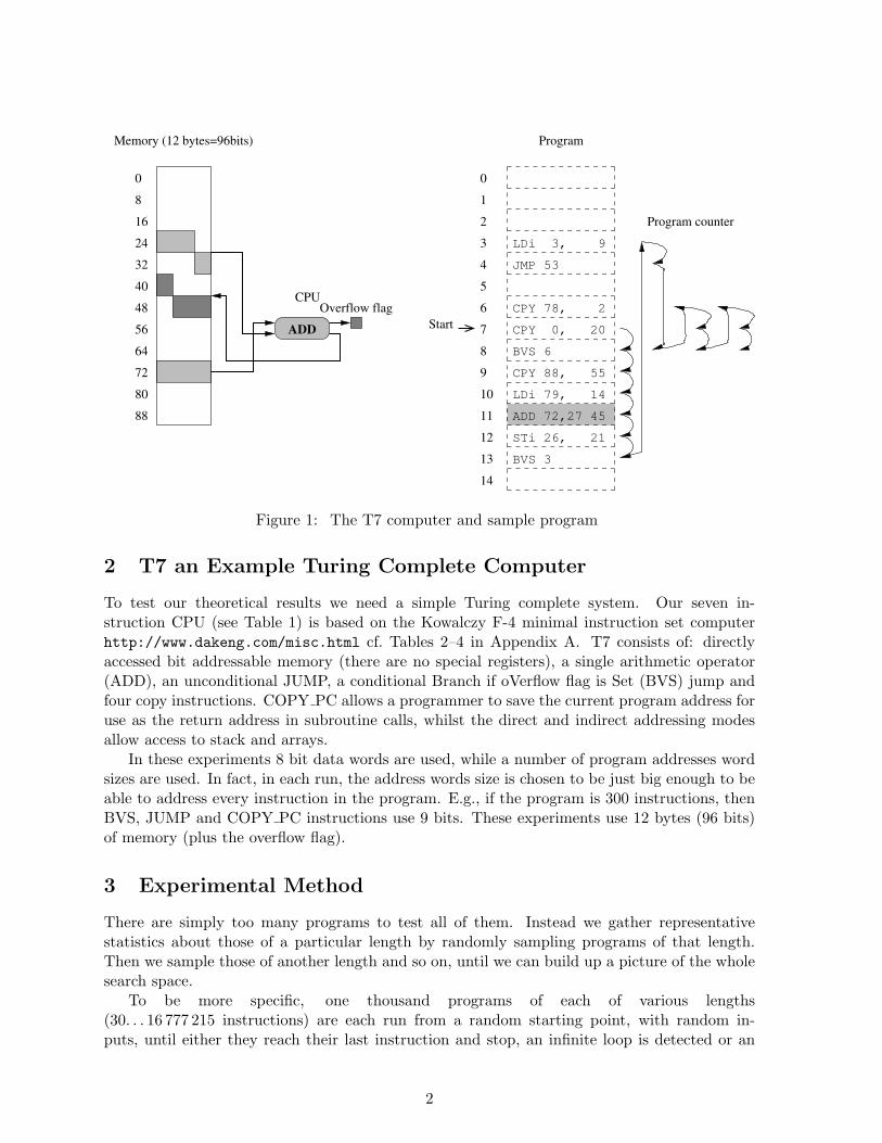
Figure 1: The T7 computer and sample program

2 T7 an Example Turing Complete Computer

To test our theoretical results we need a simple Turing complete system. Our seven in-struction CPU (see Table 1) is based on the Kowalczy F-4 minimal instruction set computerhttp://www.dakeng.com/misc.html cf. Tables 2–4 in Appendix A. T7 consists of: directlyaccessed bit addressable memory (there are no special registers), a single arithmetic operator(ADD), an unconditional JUMP, a conditional Branch if oVerflow flag is Set (BVS) jump andfour copy instructions. COPY PC allows a programmer to save the current program address foruse as the return address in subroutine calls, whilst the direct and indirect addressing modesallow access to stack and arrays.

In these experiments 8 bit data words are used, while a number of program addresses wordsizes are used. In fact, in each run, the address words size is chosen to be just big enough to beable to address every instruction in the program. E.g., if the program is 300 instructions, thenBVS, JUMP and COPY PC instructions use 9 bits. These experiments use 12 bytes (96 bits)of memory (plus the overflow flag).

3 Experimental Method

There are simply too many programs to test all of them. Instead we gather representativestatistics about those of a particular length by randomly sampling programs of that length.Then we sample those of another length and so on, until we can build up a picture of the wholesearch space.

To be more specific, one thousand programs of each of various lengths(30. . . 16 777 215 instructions) are each run from a random starting point, with random in-puts, until either they reach their last instruction and stop, an infinite loop is detected or an

2

Instruction #operands operation v setADD 3 A + B→C vBVS 1 #addr→pc if v=1COPY 2 A→BLDi 2 @A→BSTi 2 A→@BCOPY PC 1 pc→AJUMP 1 addr→pc

Each operation has up to three arguments. These are valid addresses of memory locations.Every ADD operation either sets or clears the overflow bit v. LDi and STi, treat one of theirarguments as the address of the data. They allow array manipulation without the need forself modifying code. cf. Table 4. (LDi and STi data addresses are 8 bits.) To ensure JUMPaddresses are legal, they are reduced modulo the program length.

Table 1: T7 Turing Complete Instruction Set

individual instruction has been executed more than 100 times. (In practise we can detect almostall infinite loops by keeping track of the machine’s contents, i.e. memory and overflow bit. Wecan be sure the loop is infinite, if the contents is identical to what it was when the instructionwas last executed.) The programs’ execution paths are then analysed. Statistics are gatheredon the number of instructions executed, normal program terminations, type of loops, length ofloops, start of first loop, etc.

4 Terminating Programs

The introduction of Turing completeness into GP raises the halting problem, in particular howto assign fitness to a program which may loop indefinitely [8]. We shall give a lower bound onthe number of programs which, given arbitrary input, stop, and show how this varies with theirsize.

The T7 instruction set has been designed to have as little bias as possible. In particular, givena random starting point a random sequence of ADD and copy instructions will create anotherrandom pattern in memory. The contents of the memory is essentially uniformly random. I.e.the overflow v bit is equally likely to be set as to be clear, and each address in memory isequally likely. (Where programs are not exactly a fraction of a power of two long, JUMPand COPY PC addresses cannot completely fill the number of bits allocated to them. Thisintroduces a slight bias in favour of lower addresses.) So, until correlations are introducedby re-executing the same instructions, we can treat JUMP instructions as being to randomlocations in the program. Similarly we can treat half BVS as jumping to a random address.The other half do nothing. We will start by analysing the simplest case of a loop formed byrandom jumps. First we present an accurate Markov chain model, then Section 4.2 gives aless precise but more mathematical model. Section 4.3 considers the run time of terminatingprograms.

3

1/75/71/2

SINKHALT

1/7

SINKHALT

1/2

state i=L

1−1/L 1−1/L

HALT

SINK SINK SINK

SINK

HALT

1/2

SINK

1−1/L

5/7 1/7 1/7

1/L1/L

no jump BVSJUMP

not lastlast

did jump

state i+1

state i+1

state i+1

state i

(L−i)/L

1−(L−i)/L(L−i)/L

1−(L−i)/L

1/2

(L−i)/L 1−(L−i)/L

last not last1/L

last not last

J=floor(i*3/14)AJ=max(J−((J+1)*J/2)/(L−i),0)

did not jump(L−1−i−AJ)/(L−1−i)

1−(L−1−i−AJ)/(L−1−i)

state i+1

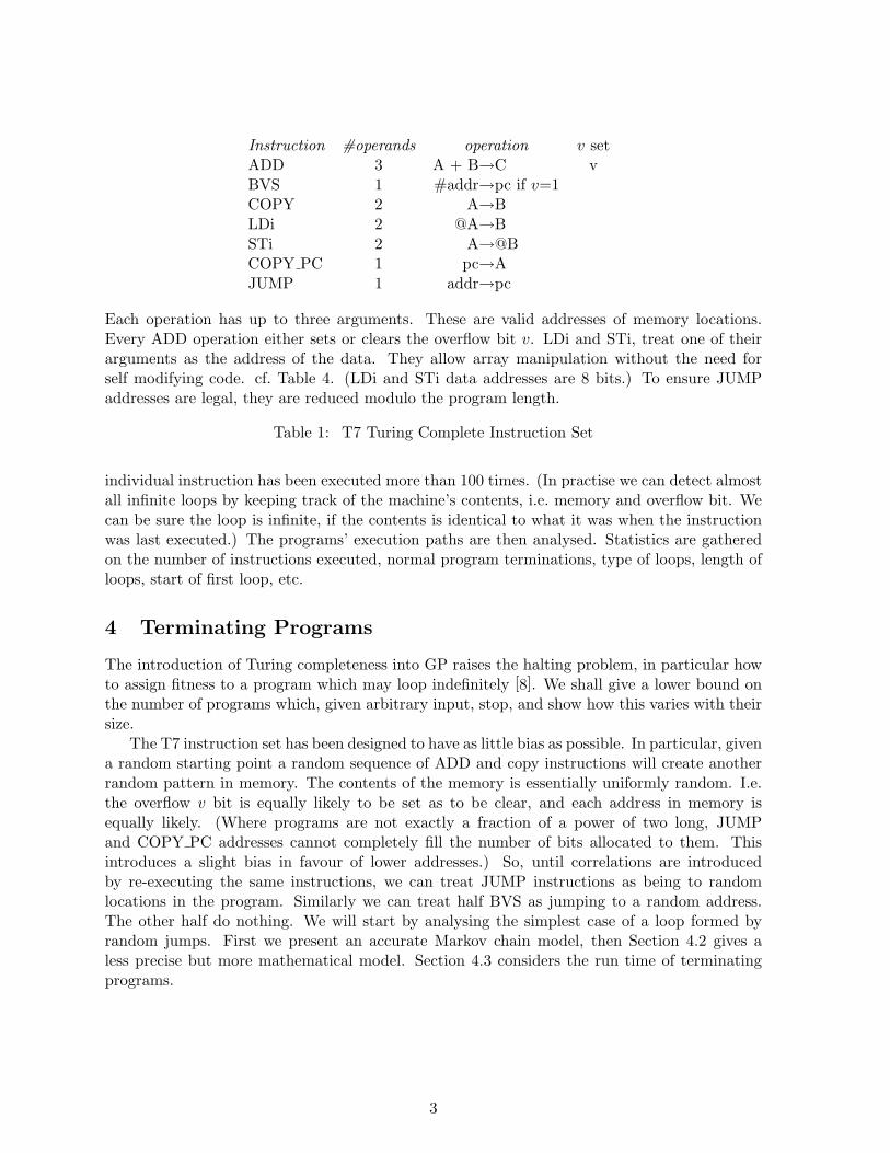
Figure 2: Probability tree used to create Markov model of the execution of random Turingcomplete programs. HALT indicates a terminating program, while SINK means the start of aloop.

4.1 Markov Chain Model of Non-Looping Programs

The Markov chain model predicts how many programs will not loop and so halt. This meansit, and the following segments model, do not take into account those programs which are ableto escape loops and do reach the end of the program and stop. As a program runs, the modelkeeps track of: the number of new instructions it executes, if it has repeated any, and if ithas stopped. The last two states are attractors from which the Markov process cannot escape.State i means the program has run i instructions without repeating any. The next instructionwill take the program from state i either to state i + 1, to SINK or to HALT. In our modelthe probabilities of each of these transitions depends only on i and the program length L,see Figure 2. We construct a (L + 2) × (L + 2) Markov transition matrix T containing theprobabilities in Figure 2. The probabilities of reaching the end of the program (HALT) or thelooping (SINK) are given by two entries in TL. Figure 3 shows our Markov chain describes thefraction of programs which never repeat any instructions very well.

4.2 Segment Model of Non-Looping Programs

As before, we assume half BVS instructions cause a jump. So the chance of program flow notbeing disrupted is 11/14. Thus the average length of uninterrupted random sequential instruc-tions is

∑L/2i=1 i (11/14)i−1 3/14. We can reasonably replace the upper limit on the summation

by infinity to give the geometric distribution (mean of 14/3 = 4.67 and standard deviation√142/32 × 11/3 = 8.94).For simplicity we will assume the program’s L instructions are divided into L/4.67 segments.

Two thirds end with a JUMP and the remainder with an active BVS (i.e. with the overflow

4

0.001

0.01

0.1

1

100 1000 10000 100000 1e+06 1e+07

Frac

tion

Program length

Programs known not to HaltPrograms which Halt

Programs which never loopPrograms which might Halt

Markov modelSegments Model

2.13/sqrt(x)

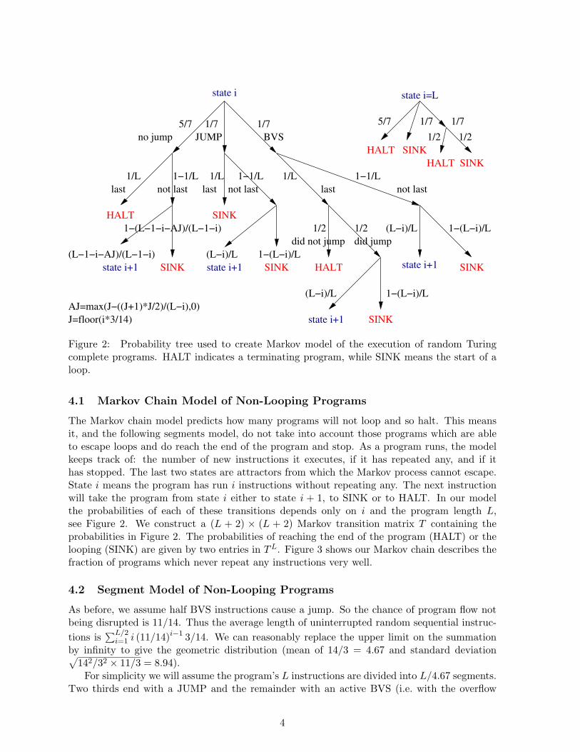
Figure 3: Looping + and terminating (2 ) T7 programs To smooth these two curves, 50 000to 200 000 samples taken at exact powers of two. (Other lengths lie slightly below these curves).Solid diagonal line is the Markov model of programs without any repeated instructions. Thisapproximately fits , especially if lengths are near a power of two. The other diagonal line isthe segments model and its large program limit, 2.13 length−

12 . The small number of programs

which did not halt, but which might do so eventually, are also plotted ×.

bits set). The idea behind this simplification is that if we jump to any of the instructions ina segment, the normal sequencing of (i.e. non-branching) instructions will carry us to its end,thus guaranteeing the last instruction will be executed. The chance of jumping to a segmentthat has already been executed is the ratio of already executed segments to the total. (Thisignores the possibility that the last instruction is a jump. We compensate for this later.)

Let i be the number of instructions run so far divided by 4.67 and N = L/4.67. At the endof each segment, there are three possible outcomes: either we jump to the end of the program(probability 1/N) and so stop its execution; we jump to a segment that has already been run(probability i/N) so forming a loop; or we branch elsewhere. The chance the program repeatsan instruction at the end of the ith segment is

=i

N(1− 2

N)(1− 3

N) . . . (1− i

N)

I.e. it is the chance of jumping back to code that has already been executed (i/N) times theprobability we have not already looped or exited the program at each of the previous steps.Similarly the chance the program stops at the end of the ith segment is

1N

(1− 2N

)(1− 3N

) . . . (1− i

N) =

1N i

(N − 2)!(N − i− 1)!

=(N − 2)!NN−1

NN−1−i

(N − i− 1)!

= (N − 2)!N1−NeNPsn(N − i− 1, N)

Where Psn(k, λ) = e−λλk/k! is the Poisson distribution with mean λ.

5

0

0.02

0.04

0.06

0.08

0.1

0.12

0.14

0.16

0.18

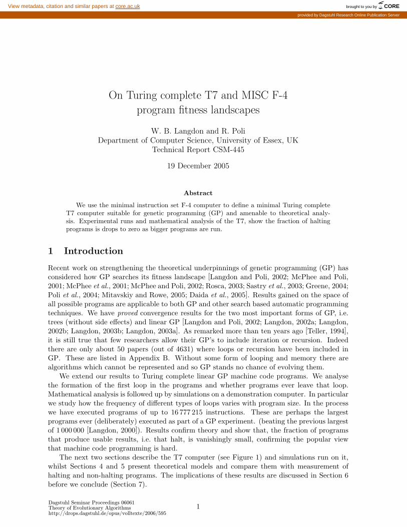
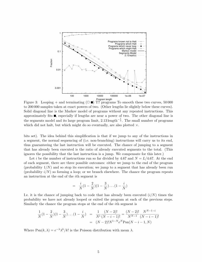
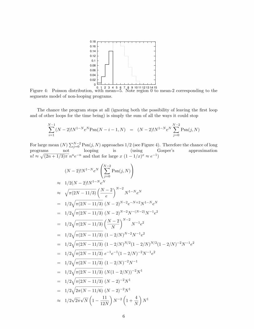
0 1 2 3 4 5 6 7 8 9 10 11 12 13 14 15Figure 4: Poisson distribution, with mean=5. Note region 0 to mean-2 corresponding to thesegments model of non-looping programs.

The chance the program stops at all (ignoring both the possibility of leaving the first loopand of other loops for the time being) is simply the sum of all the ways it could stop

N−1∑i=1

(N − 2)!N1−NeNPsn(N − i− 1, N) = (N − 2)!N1−NeNN−2∑j=0

Psn(j,N)

For large mean (N)∑N−2

j=0 Psn(j, N) approaches 1/2 (see Figure 4). Therefore the chance of longprograms not looping is (using Gosper’s approximationn! ≈

√(2n + 1/3)π nne−n and that for large x (1− 1/x)x ≈ e−1)

(N − 2)!N1−NeN

N−2∑j=0

Psn(j,N)

≈ 1/2(N − 2)!N1−NeN

≈√

π(2N − 11/3)(

N − 2e

)N−2

N1−NeN

= 1/2√

π(2N − 11/3) (N − 2)N−2e−N+2N1−NeN

= 1/2√

π(2N − 11/3) (N − 2)N−2N−(N−2)N−1e2

= 1/2√

π(2N − 11/3)(

N − 2N

)N−2

N−1e2

= 1/2√

π(2N − 11/3) (1− 2/N)N−2N−1e2

= 1/2√

π(2N − 11/3) (1− 2/N)N/2(1− 2/N)N/2(1− 2/N)−2N−1e2

= 1/2√

π(2N − 11/3) e−1e−1(1− 2/N)−2N−1e2

= 1/2√

π(2N − 11/3) (1− 2/N)−2N−1

= 1/2√

π(2N − 11/3) (N(1− 2/N))−2N1

= 1/2√

π(2N − 11/3) (N − 2)−2N1

= 1/2√

2π(N − 11/6) (N − 2)−2N1

≈ 1/2√

2π√

N

(1− 11

12N

)N−2

(1 +

4N

)N1

6

= 1/2√

2πN−0.5(

1− 1112N

)(1 +

4N

)= 1/2

√2π/N

(1− 11

12N

)(1 +

4N

)≈ 1/2

√2π/N

(1 +

48− 1112N

)≈ 1/2

√2π/N

(1 +

3712N

)That is (ignoring both the possibility of leaving the first loop and of other loops for thetime being) the probability of a long random T7 program of length L stopping is about1/2

√2π14/3L

(1 + 37×14

36L

)=√

7π/3L (1 + 259/18L). As mentioned above, we have to con-sider explicitly the 3/14 of programs where the last instruction is itself an active jump. In-cluding this correction gives the chance of a long program not repeating any instructions as≈ 11/14

√7π/3L (1 + 259/18L). Figure 3 shows this

√length scaling fits the data reasonably

well.

4.3 Average Number of Instructions run before Stopping

The average number of instructions run before stopping can easily be computed from the Markovchain. This gives an excellent fit with the data (Figure 5). However, to get a scaling law, weagain apply our segments model.

The mean number of segments evaluated by programs that do halt is:∑N−1i=1 i/N

∏ij=2(1− j/N)∑N−1

i=1 1/N∏i

j=2(1− j/N)

Consider the top term for the time being

N−1∑i=1

i/Ni∏

j=2

(1− j/N)

= 1/NN−1∑i=1

i exp

i∑j=2

log(1− j/N)

< 1/N

N−1∑i=1

i exp

i∑j=2

−j/N

= 1/N

N−1∑i=1

i exp(− i(i + 1)− 2

2N

)

= 1/NN−1∑i=1

i exp

(− i2

2N

)exp

(− i

2N

)exp

(+22N

)

= 1/Ne1N

N−1∑i=1

i exp

(− i2

2N

)exp

(− i

2N

)

< 1/Ne1N e−

12N

N−1∑i=1

i exp

(− i2

2N

)

7

= e1

2N 1/NN−1∑i=1

i exp

(− i2

2N

)

≈ e1

2N 1/N

∫ N−1/2

1/2xe−x2/2Ndx

= e1

2N 1/N[−Ne−x2/2N

]N−1/2

1/2

= e1

2N

[e−x2/2N

]1/2

N−1/2

= e1

2N

(e−1/8N − e−(N−1/2)2/2N

)≈ e

38N

Dividing e3

8N by the lower part (the probability of a long program not looping) gives anupper bound on the expected number of segments executed by a program which does not entera loop:

≈ e3/8N

1/2√

2π/N(1 + 37

12N

)≈ 2(1 + 3/8N)(1− 37/12N)

√N/2π

≈ (1 + 9/24N − 74/24N)√

2N/π

= (1− 65/24N)√

2N/π

≈ 0.8√

N

Replacing the number of segments N (N = 3L/14) by the the number of instructions Lgives 14/3 ×

√2/π

√3/14

√L =

√28/3π

√L ≈ 1.72

√L. Figure 5 shows, particularly for large

random programs, this gives a good bound for the T7 segments model. However the segmentsmodel itself is an over estimate.

Neither the segments model, nor the Markov model, take into account de-randomisation ofmemory as more instructions are run. This is particularly acute since we have a small memory.JUMP and COPY PC instructions introduce correlations between the contents of memory andthe path of the program counter. These make it easier for loops to form.

4.4 How random is memory?

Our models assume that the contents of memory is random. Figure 6 shows this assumptionis valid initially. However as random instructions are executed the number of bits set tends towonder away from its initial setting, cf. Figure 7. Where legal program addresses do not fitexactly into the power of two allocated to them, the upper bits of random addresses are morelikely to be zero than 1/2. This means COPY PC instructions tend to inject more zeros intomemory. This leads to the slight asymmetry seen in one plot in Figure 6. Figure 8 shows thatwhile memory appears random at a given time, its contents is correlated from one time to thenext. A simple model based on the chance of random instructions over writing addresses storedin memory predicts, in large programs, an address will survive on average ≈ 5 instructions.

8

1

10

100

1000

1 10 100 1000 10000 100000 1e+06 1e+07

Mea

n ev

alua

ted

inst

ruct

ions

by

halti

ng p

roga

ms

Program length

Mean (standard error) instructions executed ( may loop )Mean (standard error) instructions executed (no repeats)

1.72 sqrt(x)Segments Model

Markov model

Figure 5: Instructions executed by programs which halt. Standard deviations are approximatelyequal to the means, suggesting geometric distributions. As Figure 3, larger samples used toincrease reliability. Models reasonable for short programs. However as random programs runfor longer, COPY PC and JUMP derandomise the small memory, so easing looping.

1

10

100

0 8 16 24 32 40 48 56 64 72 80 88 96

Num

ber o

f ran

dom

pro

gram

s (to

tal 1

000)

Number of bits set in memory

Length=2^23 Mean=43.8, SD=9.4 Length=2^24-1 Mean=47.1, SD=9.1

Gaussian(48,4.9)Initial

Program length=2^23Program length=2^24-1

Figure 6: We count the number of bits set in memory when a random program terminates orfirst repeats an instruction. (Remember the longer random programs tend to execute more suchinstructions). Random instructions tend to derandomise the memory only a little. However noteprograms of length 223 (dashed line) never use the most significant bit of their 24 bit addresses.This gives and a slightly asymmetric distribution, not visible for programs of length 224 − 1(dotted line).

9

4

5

6

7

8

9

10

1 10 100 1000 10000 100000 1e+06 1e+07

Spr

ead

of n

umbe

r of b

its s

et in

mem

ory

Program size

Standard deviation at end progInitial standard deviation

Random

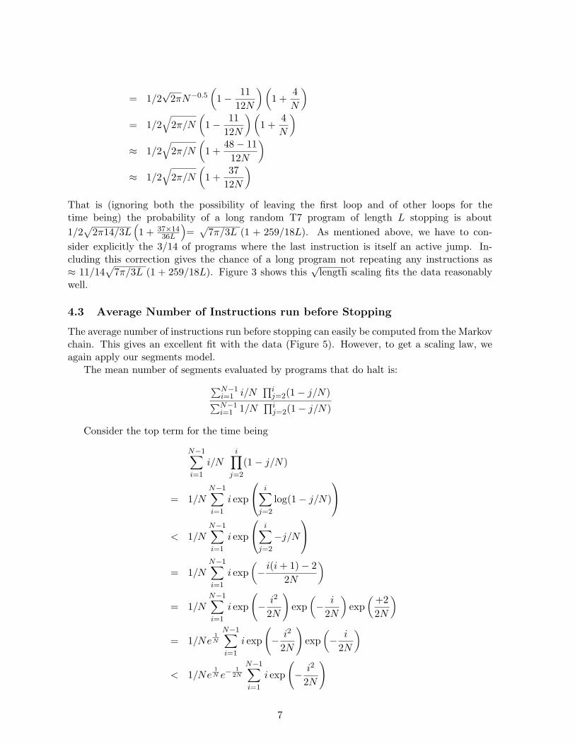
Figure 7: Spread of number of bits set in 1000 random programs, cf. Figure 6. Longer randomprograms tend to run more instructions before either stopping or repeating an instruction. Thiscauses the memory to derandomise only a little. This plot shows, for large random programs,the spread in number of bits set in memory is up to twice that which would be expected ofrandom initial fluctuations.

0

20

40

60

80

100

120

140

160

180

200

1 10 100 1000 10000 100000 1e+06 1e+07Mea

n an

d S

tand

ard

Dev

iatio

n of

life

tim

e of

add

ress

es in

mem

ory

Program size

Mean number of copies over program execution (until first loop)(7.0*M)/(4*(d+a-1-3)+(a+a-1-3)) plus small prog corrections

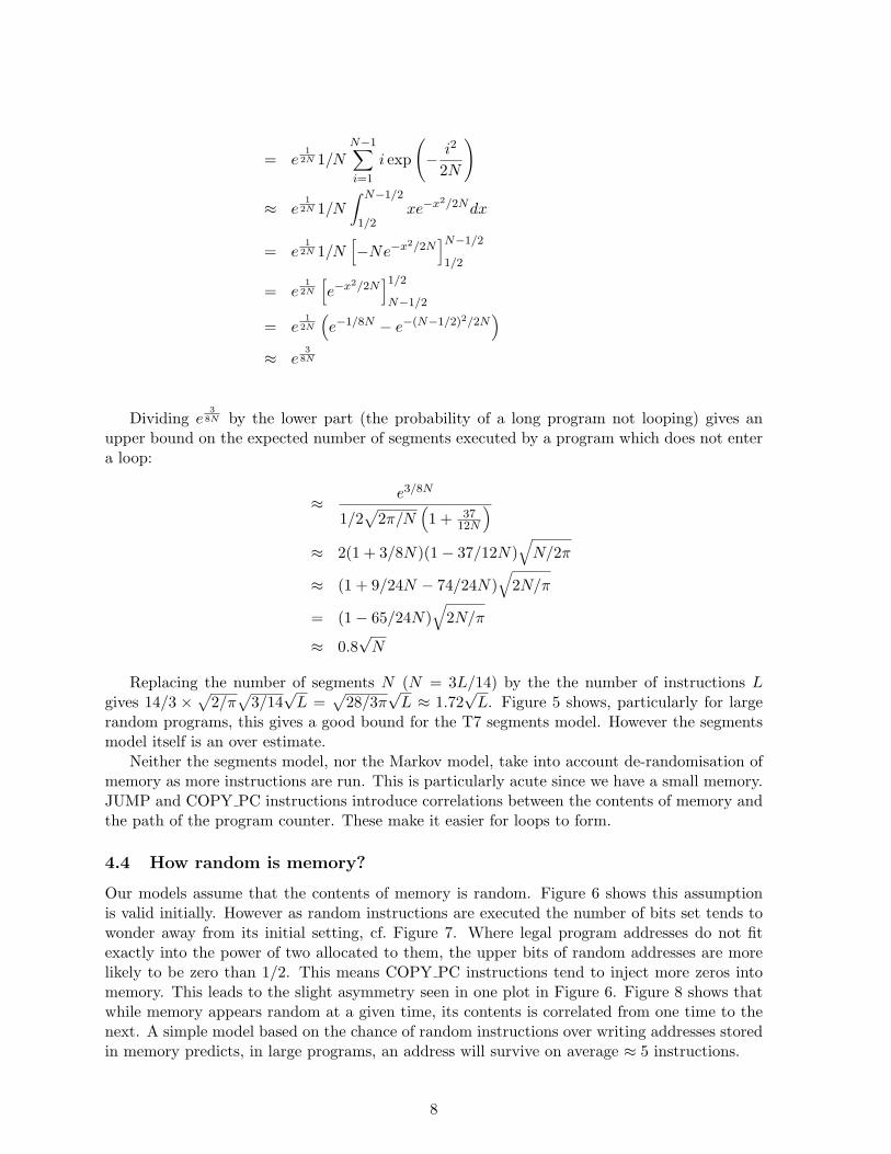
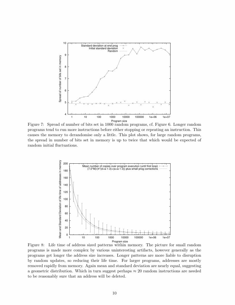
Figure 8: Life time of address sized patterns within memory. The picture for small randomprograms is made more complex by various uninteresting artifacts, however generally as theprograms get longer the address size increases. Longer patterns are more liable to disruptionby random updates, so reducing their life time. For larger programs, addresses are mostlyremoved rapidly from memory. Again mean and standard deviation are nearly equal, suggestinga geometric distribution. Which in turn suggest perhaps ≈ 20 random instructions are neededto be reasonably sure that an address will be deleted.

10

0

50

100

150

200

250

300

350

400

450

500

10 100 1000 10000 100000 1e+06 1e+07

Cou

nt

Program length

COPY_PCJUMP

BVSOther loops

Programs which stop

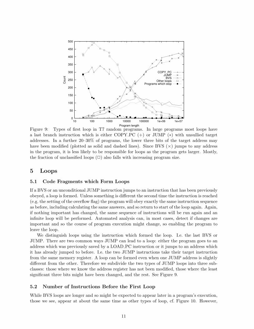
Figure 9: Types of first loop in T7 random programs. In large programs most loops havea last branch instruction which is either COPY PC (+) or JUMP (∗) with unsullied targetaddresses. In a further 20–30% of programs, the lower three bits of the target address mayhave been modified (plotted as solid and dashed lines). Since BVS (×) jumps to any addressin the program, it is less likely to be responsible for loops as the program gets larger. Mostly,the fraction of unclassified loops (2) also falls with increasing program size.

5 Loops

5.1 Code Fragments which Form Loops

If a BVS or an unconditional JUMP instruction jumps to an instruction that has been previouslyobeyed, a loop is formed. Unless something is different the second time the instruction is reached(e.g. the setting of the overflow flag) the program will obey exactly the same instruction sequenceas before, including calculating the same answers, and so return to start of the loop again. Again,if nothing important has changed, the same sequence of instructions will be run again and aninfinite loop will be performed. Automated analysis can, in most cases, detect if changes areimportant and so the course of program execution might change, so enabling the program toleave the loop.

We distinguish loops using the instruction which formed the loop. I.e. the last BVS orJUMP. There are two common ways JUMP can lead to a loop: either the program goes to anaddress which was previously saved by a LOAD PC instruction or it jumps to an address whichit has already jumped to before. I.e. the two JUMP instructions take their target instructionfrom the same memory register. A loop can be formed even when one JUMP address is slightlydifferent from the other. Therefore we subdivide the two types of JUMP loops into three sub-classes: those where we know the address register has not been modified, those where the leastsignificant three bits might have been changed, and the rest. See Figure 9.

5.2 Number of Instructions Before the First Loop

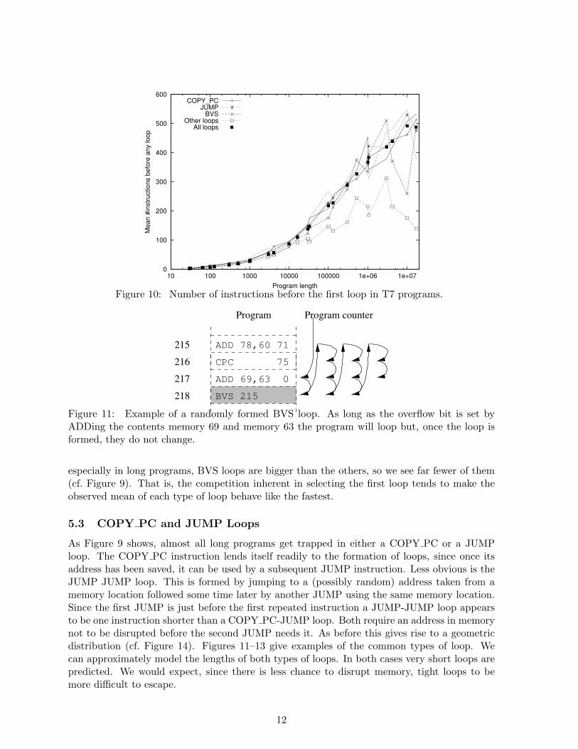
While BVS loops are longer and so might be expected to appear later in a program’s execution,those we see, appear at about the same time as other types of loop, cf. Figure 10. However,

11

0

100

200

300

400

500

600

10 100 1000 10000 100000 1e+06 1e+07

Mea

n #i

nstru

ctio

ns b

efor

e an

y lo

op

Program length

COPY_PCJUMP

BVSOther loops

All loops

Figure 10: Number of instructions before the first loop in T7 programs.

217

218

215

216

Program Program counter

BVS 215

CPC 75

ADD 69,63 0

ADD 78,60 71

Figure 11: Example of a randomly formed BVS loop. As long as the overflow bit is set byADDing the contents memory 69 and memory 63 the program will loop but, once the loop isformed, they do not change.

especially in long programs, BVS loops are bigger than the others, so we see far fewer of them(cf. Figure 9). That is, the competition inherent in selecting the first loop tends to make theobserved mean of each type of loop behave like the fastest.

5.3 COPY PC and JUMP Loops

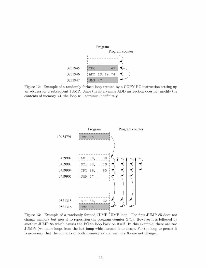
As Figure 9 shows, almost all long programs get trapped in either a COPY PC or a JUMPloop. The COPY PC instruction lends itself readily to the formation of loops, since once itsaddress has been saved, it can be used by a subsequent JUMP instruction. Less obvious is theJUMP JUMP loop. This is formed by jumping to a (possibly random) address taken from amemory location followed some time later by another JUMP using the same memory location.Since the first JUMP is just before the first repeated instruction a JUMP-JUMP loop appearsto be one instruction shorter than a COPY PC-JUMP loop. Both require an address in memorynot to be disrupted before the second JUMP needs it. As before this gives rise to a geometricdistribution (cf. Figure 14). Figures 11–13 give examples of the common types of loop. Wecan approximately model the lengths of both types of loops. In both cases very short loops arepredicted. We would expect, since there is less chance to disrupt memory, tight loops to bemore difficult to escape.

12

3233945

3233946

3233947

Program counterProgram

JMP 47

CPC 47

ADD 19,49 74

Figure 12: Example of a randomly formed loop created by a COPY PC instruction setting upan address for a subsequent JUMP. Since the intervening ADD instruction does not modify thecontents of memory 74, the loop will continue indefinitely.

9521315

3459902

3459903

3459904

3459905

9521316

Program Program counter

10434791

JMP 27

CPY 86, 65

LDi 79, 38

STi 30, 19

JMP 85

STi 58, 62

JMP 85

Figure 13: Example of a randomly formed JUMP-JUMP loop. The first JUMP 85 does notchange memory but uses it to reposition the program counter (PC). However it is followed byanother JUMP 85 which causes the PC to loop back on itself. In this example, there are twoJUMPs (we name loops from the last jump which caused it to close). For the loop to persist itis necessary that the contents of both memory 27 and memory 85 are not changed.

13

0

100

200

300

400

500

600

0 100 200 300 400 500 600

Sta

ndar

d D

evia

tion

Mean #instructions before any loop

All loops

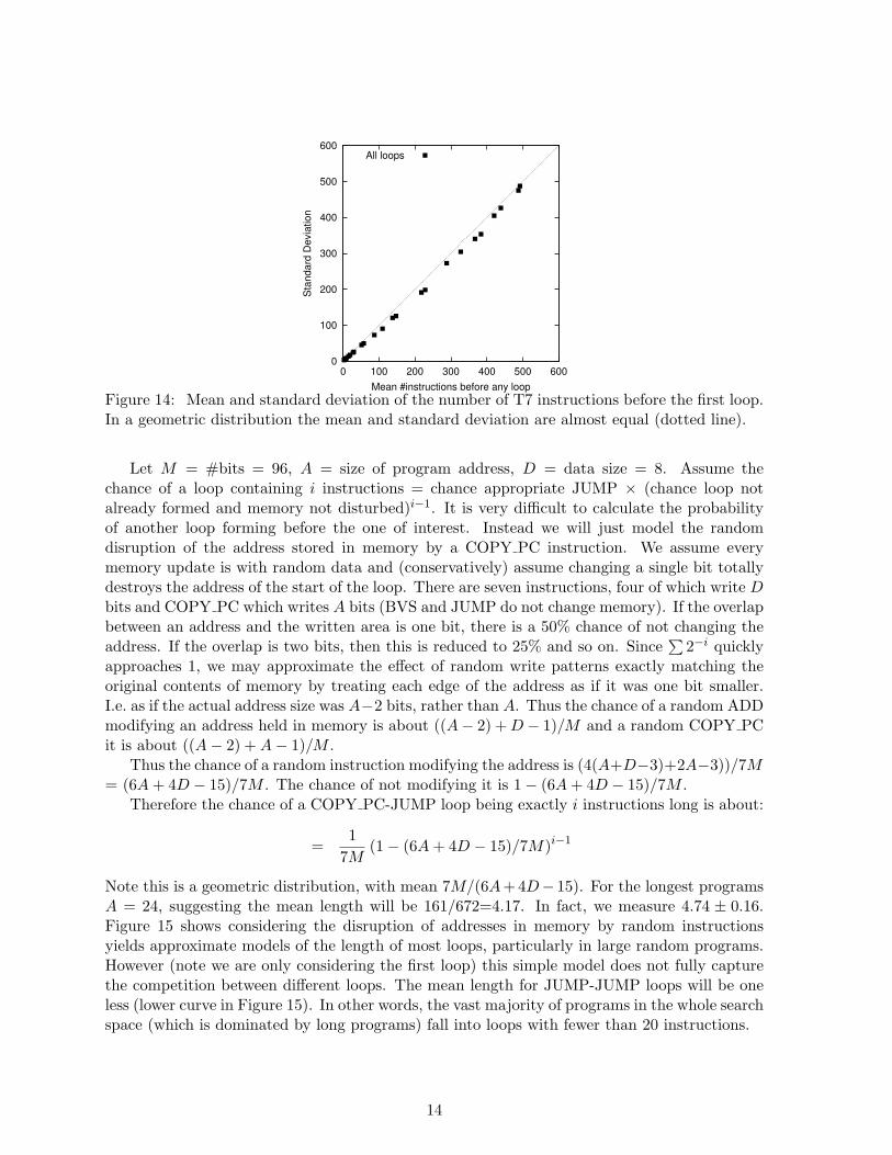
Figure 14: Mean and standard deviation of the number of T7 instructions before the first loop.In a geometric distribution the mean and standard deviation are almost equal (dotted line).

Let M = #bits = 96, A = size of program address, D = data size = 8. Assume thechance of a loop containing i instructions = chance appropriate JUMP × (chance loop notalready formed and memory not disturbed)i−1. It is very difficult to calculate the probabilityof another loop forming before the one of interest. Instead we will just model the randomdisruption of the address stored in memory by a COPY PC instruction. We assume everymemory update is with random data and (conservatively) assume changing a single bit totallydestroys the address of the start of the loop. There are seven instructions, four of which write Dbits and COPY PC which writes A bits (BVS and JUMP do not change memory). If the overlapbetween an address and the written area is one bit, there is a 50% chance of not changing theaddress. If the overlap is two bits, then this is reduced to 25% and so on. Since

∑2−i quickly

approaches 1, we may approximate the effect of random write patterns exactly matching theoriginal contents of memory by treating each edge of the address as if it was one bit smaller.I.e. as if the actual address size was A−2 bits, rather than A. Thus the chance of a random ADDmodifying an address held in memory is about ((A− 2) + D − 1)/M and a random COPY PCit is about ((A− 2) + A− 1)/M .

Thus the chance of a random instruction modifying the address is (4(A+D−3)+2A−3))/7M= (6A + 4D − 15)/7M . The chance of not modifying it is 1− (6A + 4D − 15)/7M .

Therefore the chance of a COPY PC-JUMP loop being exactly i instructions long is about:

=1

7M(1− (6A + 4D − 15)/7M)i−1

Note this is a geometric distribution, with mean 7M/(6A+4D− 15). For the longest programsA = 24, suggesting the mean length will be 161/672=4.17. In fact, we measure 4.74 ± 0.16.Figure 15 shows considering the disruption of addresses in memory by random instructionsyields approximate models of the length of most loops, particularly in large random programs.However (note we are only considering the first loop) this simple model does not fully capturethe competition between different loops. The mean length for JUMP-JUMP loops will be oneless (lower curve in Figure 15). In other words, the vast majority of programs in the whole searchspace (which is dominated by long programs) fall into loops with fewer than 20 instructions.

14

1

10

100

1000

10 100 1000 10000 100000 1e+06 1e+07

Mea

n #i

nstru

ctio

ns in

firs

t loo

p

Program length

COPY_PCJUMP

BVSOther loops

All loopsCOPY_PC-JUMP model

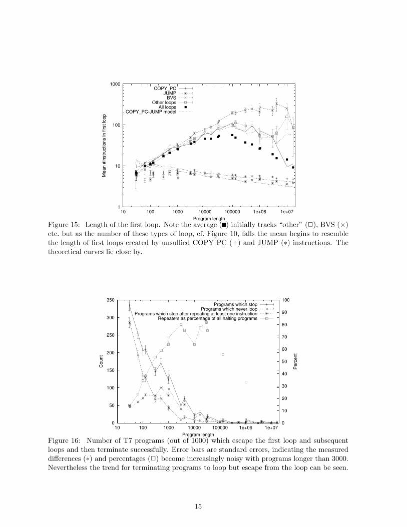
Figure 15: Length of the first loop. Note the average ( ) initially tracks “other” (2), BVS (×)etc. but as the number of these types of loop, cf. Figure 10, falls the mean begins to resemblethe length of first loops created by unsullied COPY PC (+) and JUMP (∗) instructions. Thetheoretical curves lie close by.

0

50

100

150

200

250

300

350

10 100 1000 10000 100000 1e+06 1e+070

10

20

30

40

50

60

70

80

90

100

Cou

nt

Per

cent

Program length

Programs which stopPrograms which never loop

Programs which stop after repeating at least one instructionRepeaters as percentage of all halting programs

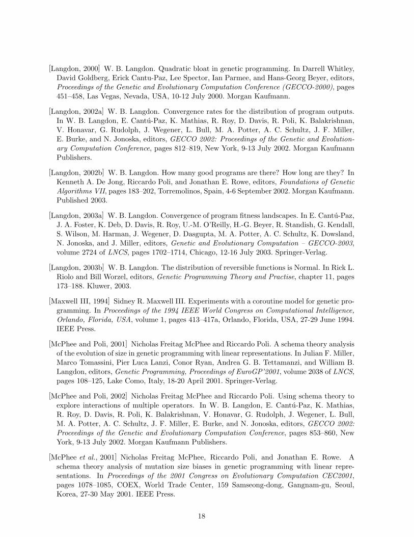
Figure 16: Number of T7 programs (out of 1000) which escape the first loop and subsequentloops and then terminate successfully. Error bars are standard errors, indicating the measureddifferences (∗) and percentages (2) become increasingly noisy with programs longer than 3000.Nevertheless the trend for terminating programs to loop but escape from the loop can be seen.

15

6 Discussion

Of course the undecidability of the Halting problem has long been known. More recently workby Chaitin [Chaitin, 1988] started to consider a probabilistic information theoretic approach.However this is based on self-delimiting Turing machines (particularly the “Chaitin machines”)and has lead to a non-zero value for Ω [Calude et al., 2002] and postmodern metamathematics.Our approach is firmly based on the von Neumann architecture, which for practical purposesis Turing complete. Indeed the T7 computer is similar to the linear GP area of existing Turingcomplete GP research.

While the numerical values we have calculated are specific to the T7, the scaling lawsare general. Given time and resources it would be nice to perform similar experiments withmore memory and on different computers. Obviously include a halt instruction will change theproportions radically but leads to many random programs terminating but having run only ahandful of instructions. Our results are also very general in the sense that they apply to thespace of all possible programs and so are applicable to both GP and any other search basedautomatic programming techniques.

Section 4 has accurately modelled the formation of the first loops in program execution.Section 5 shows in long programs most loops are quite short but we have not yet been able toquantitatively model the programs which enter a loop and then leave it. However we can arguerecursively that once the program has left a loop it is back almost where it started. That is,it has executed only a tiny fraction of the whole program, and the remainder is still randomwith respect to its current state. Now there may be something in the memory which makes itto easier to exit loops, or harder to form them in the first place. For example, the overflow flagnot being set. However we would expect the flag to be randomised almost immediately. Alsoinitial studies, c.f. Section 4.4, indicate the rest of the memory remains randomised. That ishaving left one loop, we expect the chance of entering another to be much the same as whenthe program started, i.e. almost one. Thus the program will stumble from one loop to anotheruntil it gets trapped by a loop it cannot escape. As explained in Section 5, we expect, in longprograms, it will not take long to find a short loop from which it is impossible to escape.

Real computer systems lose information (converting into heat). We expect this to lead tofurther convergence properties in programming languages with recursion and memory.

7 Conclusions

Our models and simulations of a Turing complete linear GP system based on practical von Neu-mann computer architectures, show that the proportion of halting programs falls towards zerowith increasing program length. However there are exponentially more long programs thanshort ones. This means in absolute terms the number of halting programs increases with theirsize (cf. Figure 17) but, in probabilistic terms, the Halting problem is decidable: von Neumannprograms do not terminate with probability one.

In detail: the proportion of halting programs is ≈ 1/√

length, while the average and standarddeviation of the run time of terminating programs grows as

√length. This suggests a limit on run

time of, say, 20 times√

length instruction cycles, will differentiate between almost all haltingand non-halting T7 programs. E.g. for a real GHz machine, if a random program has beenrunning for a single millisecond that is enough to be confident that it will never stop.

16

100

1000

10000

100000

1e+06

1e+07

1e+08

1e+09

100 1000 10000 100000 1e+06 1e+07

Log

10 C

ount

Program length

Programs which stop (lower bound)

Figure 17: The number of Halting programs rises exponentially with length despite gettingincreasingly rare as a fraction of all programs.

Acknowledgements

I would like to thank Dave Kowalczy. Funded by EPSRC grant GR/T11234/01.

References

[Calude et al., 2002] Cristian S. Calude, Michael J. Dinneen, and Chi-Kou Shu. Computing aglimpse of randomness. Experimental Mathematics, 11(3):361–370, 2002.

[Chaitin, 1988] Gregory J. Chaitin. An algebraic equation for the halting probability. In RolfHerken, editor, The Universal Turing Machine A Half-Century Survey, pages 279–283. OxfordUniversity Press, 1988.

[Daida et al., 2005] Jason M. Daida, Adam M. Hilss, David J. Ward, and Stephen L. Long.Visualizing tree structures in genetic programming. Genetic Programming and EvolvableMachines, 6(1):79–110, March 2005.

[Greene, 2004] William A. Greene. Schema disruption in chromosomes that are structuredas binary trees. In Kalyanmoy Deb, Riccardo Poli, Wolfgang Banzhaf, Hans-Georg Beyer,Edmund Burke, Paul Darwen, Dipankar Dasgupta, Dario Floreano, James Foster, MarkHarman, Owen Holland, Pier Luca Lanzi, Lee Spector, Andrea Tettamanzi, Dirk Thierens,and Andy Tyrrell, editors, Genetic and Evolutionary Computation – GECCO-2004, Part I,volume 3102 of Lecture Notes in Computer Science, pages 1197–1207, Seattle, WA, USA,26-30 June 2004. Springer-Verlag.

[Kowalczyk, 2005] Dave Kowalczyk. Programming array access F-4 MISC, October 2005. Per-sonal communication.

[Langdon and Poli, 2002] W. B. Langdon and Riccardo Poli. Foundations of Genetic Program-ming. Springer-Verlag, 2002.

17

[Langdon, 2000] W. B. Langdon. Quadratic bloat in genetic programming. In Darrell Whitley,David Goldberg, Erick Cantu-Paz, Lee Spector, Ian Parmee, and Hans-Georg Beyer, editors,Proceedings of the Genetic and Evolutionary Computation Conference (GECCO-2000), pages451–458, Las Vegas, Nevada, USA, 10-12 July 2000. Morgan Kaufmann.

[Langdon, 2002a] W. B. Langdon. Convergence rates for the distribution of program outputs.In W. B. Langdon, E. Cantu-Paz, K. Mathias, R. Roy, D. Davis, R. Poli, K. Balakrishnan,V. Honavar, G. Rudolph, J. Wegener, L. Bull, M. A. Potter, A. C. Schultz, J. F. Miller,E. Burke, and N. Jonoska, editors, GECCO 2002: Proceedings of the Genetic and Evolution-ary Computation Conference, pages 812–819, New York, 9-13 July 2002. Morgan KaufmannPublishers.

[Langdon, 2002b] W. B. Langdon. How many good programs are there? How long are they? InKenneth A. De Jong, Riccardo Poli, and Jonathan E. Rowe, editors, Foundations of GeneticAlgorithms VII, pages 183–202, Torremolinos, Spain, 4-6 September 2002. Morgan Kaufmann.Published 2003.

[Langdon, 2003a] W. B. Langdon. Convergence of program fitness landscapes. In E. Cantu-Paz,J. A. Foster, K. Deb, D. Davis, R. Roy, U.-M. O’Reilly, H.-G. Beyer, R. Standish, G. Kendall,S. Wilson, M. Harman, J. Wegener, D. Dasgupta, M. A. Potter, A. C. Schultz, K. Dowsland,N. Jonoska, and J. Miller, editors, Genetic and Evolutionary Computation – GECCO-2003,volume 2724 of LNCS, pages 1702–1714, Chicago, 12-16 July 2003. Springer-Verlag.

[Langdon, 2003b] W. B. Langdon. The distribution of reversible functions is Normal. In Rick L.Riolo and Bill Worzel, editors, Genetic Programming Theory and Practise, chapter 11, pages173–188. Kluwer, 2003.

[Maxwell III, 1994] Sidney R. Maxwell III. Experiments with a coroutine model for genetic pro-gramming. In Proceedings of the 1994 IEEE World Congress on Computational Intelligence,Orlando, Florida, USA, volume 1, pages 413–417a, Orlando, Florida, USA, 27-29 June 1994.IEEE Press.

[McPhee and Poli, 2001] Nicholas Freitag McPhee and Riccardo Poli. A schema theory analysisof the evolution of size in genetic programming with linear representations. In Julian F. Miller,Marco Tomassini, Pier Luca Lanzi, Conor Ryan, Andrea G. B. Tettamanzi, and William B.Langdon, editors, Genetic Programming, Proceedings of EuroGP’2001, volume 2038 of LNCS,pages 108–125, Lake Como, Italy, 18-20 April 2001. Springer-Verlag.

[McPhee and Poli, 2002] Nicholas Freitag McPhee and Riccardo Poli. Using schema theory toexplore interactions of multiple operators. In W. B. Langdon, E. Cantu-Paz, K. Mathias,R. Roy, D. Davis, R. Poli, K. Balakrishnan, V. Honavar, G. Rudolph, J. Wegener, L. Bull,M. A. Potter, A. C. Schultz, J. F. Miller, E. Burke, and N. Jonoska, editors, GECCO 2002:Proceedings of the Genetic and Evolutionary Computation Conference, pages 853–860, NewYork, 9-13 July 2002. Morgan Kaufmann Publishers.

[McPhee et al., 2001] Nicholas Freitag McPhee, Riccardo Poli, and Jonathan E. Rowe. Aschema theory analysis of mutation size biases in genetic programming with linear repre-sentations. In Proceedings of the 2001 Congress on Evolutionary Computation CEC2001,pages 1078–1085, COEX, World Trade Center, 159 Samseong-dong, Gangnam-gu, Seoul,Korea, 27-30 May 2001. IEEE Press.

18

[Mitavskiy and Rowe, 2005] Boris Mitavskiy and Jonathan E. Rowe. Boris Mitavskiy andJonathan E. Rowe. A schema-based version of Geiringer’s theorem for nonlinear geneticprogramming with homologous crossover. In Alden H. Wright, Michael D. Vose, Kenneth A.De Jong, and Lothar M. Schmitt, editors, Foundations of Genetic Algorithms 8, volume 3469of Lecture Notes in Computer Science, pages 156–175. Springer-Verlag, Berlin Heidelberg,2005.

[Poli et al., 2004] Riccardo Poli, Nicholas Freitag McPhee, and Jonathan E. Rowe. Exactschema theory and markov chain models for genetic programming and variable-length ge-netic algorithms with homologous crossover. Genetic Programming and Evolvable Machines,5(1):31–70, March 2004.

[Rosca, 2003] Justinian Rosca. A probabilistic model of size drift. In Rick L. Riolo andBill Worzel, editors, Genetic Programming Theory and Practice, chapter 8, pages 119–136.Kluwer, 2003.

[Sastry et al., 2003] Kumara Sastry, Una-May O’Reilly, David E. Goldberg, and David Hill.Building block supply in genetic programming. In Rick L. Riolo and Bill Worzel, editors,Genetic Programming Theory and Practice, chapter 9, pages 137–154. Kluwer, 2003.

[Teller, 1994] Astro Teller. Astro Teller. Turing completeness in the language of genetic pro-gramming with indexed memory. In Proceedings of the 1994 IEEE World Congress on Com-putational Intelligence, volume 1, pages 136–141, Orlando, Florida, USA, 27-29 June 1994.IEEE Press.

19

A Turing Equivalence of T7 and F-4

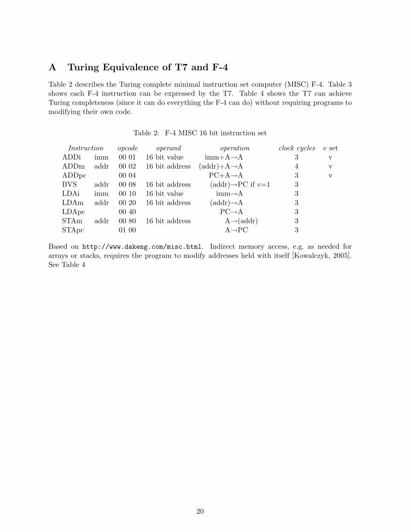
Table 2 describes the Turing complete minimal instruction set computer (MISC) F-4. Table 3shows each F-4 instruction can be expressed by the T7. Table 4 shows the T7 can achieveTuring completeness (since it can do everything the F-4 can do) without requiring programs tomodifying their own code.

Table 2: F-4 MISC 16 bit instruction set

Instruction opcode operand operation clock cycles v setADDi imm 00 01 16 bit value imm+A→A 3 vADDm addr 00 02 16 bit address (addr)+A→A 4 vADDpc 00 04 PC+A→A 3 vBVS addr 00 08 16 bit address (addr)→PC if v=1 3LDAi imm 00 10 16 bit value imm→A 3LDAm addr 00 20 16 bit address (addr)→A 3LDApc 00 40 PC→A 3STAm addr 00 80 16 bit address A→(addr) 3STApc 01 00 A→PC 3

Based on http://www.dakeng.com/misc.html. Indirect memory access, e.g. as needed forarrays or stacks, requires the program to modify addresses held with itself [Kowalczyk, 2005].See Table 4

20

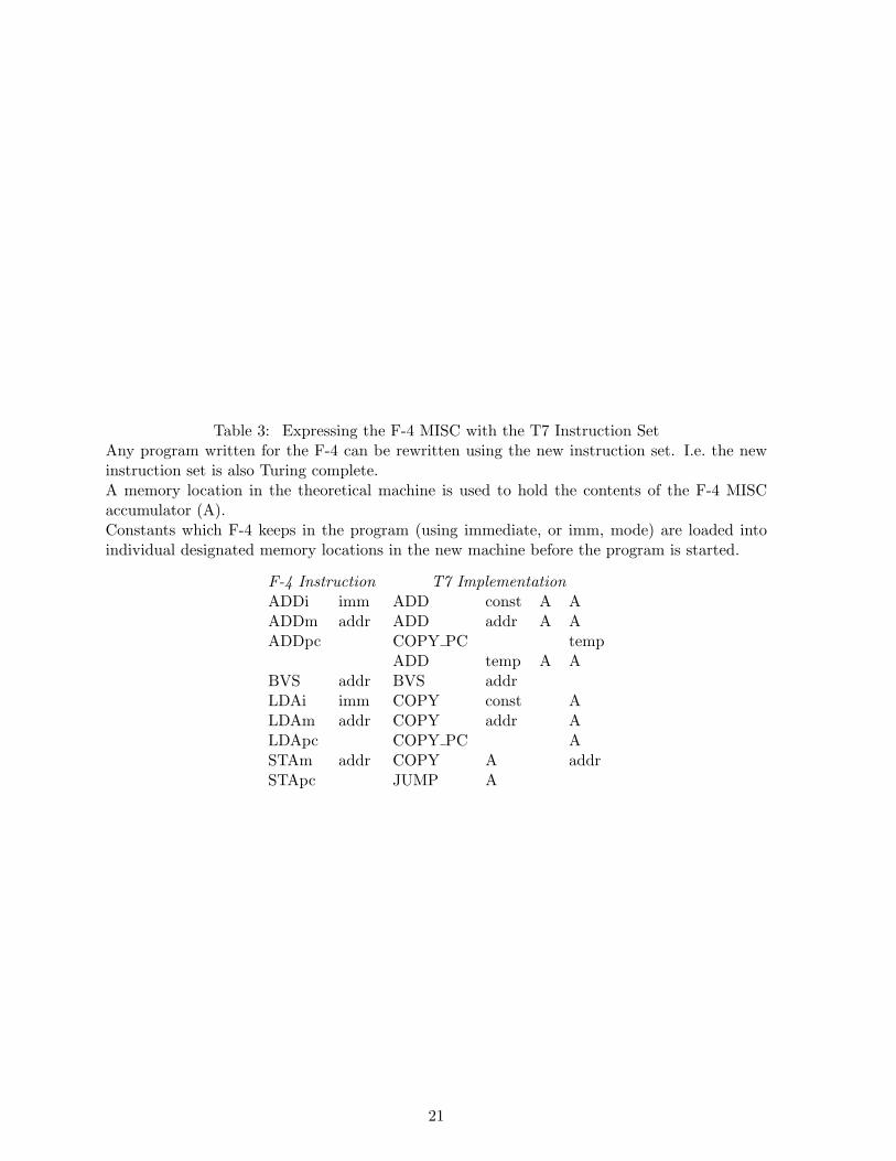
Table 3: Expressing the F-4 MISC with the T7 Instruction SetAny program written for the F-4 can be rewritten using the new instruction set. I.e. the newinstruction set is also Turing complete.A memory location in the theoretical machine is used to hold the contents of the F-4 MISCaccumulator (A).Constants which F-4 keeps in the program (using immediate, or imm, mode) are loaded intoindividual designated memory locations in the new machine before the program is started.

F-4 Instruction T7 ImplementationADDi imm ADD const A AADDm addr ADD addr A AADDpc COPY PC temp

ADD temp A ABVS addr BVS addrLDAi imm COPY const ALDAm addr COPY addr ALDApc COPY PC ASTAm addr COPY A addrSTApc JUMP A

21

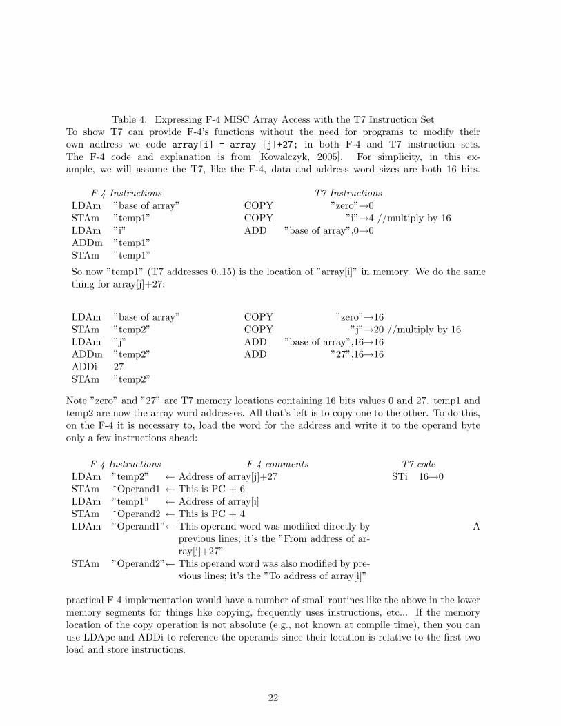
Table 4: Expressing F-4 MISC Array Access with the T7 Instruction SetTo show T7 can provide F-4’s functions without the need for programs to modify theirown address we code array[i] = array [j]+27; in both F-4 and T7 instruction sets.The F-4 code and explanation is from [Kowalczyk, 2005]. For simplicity, in this ex-ample, we will assume the T7, like the F-4, data and address word sizes are both 16 bits.

F-4 InstructionsLDAm ”base of array”STAm ”temp1”LDAm ”i”ADDm ”temp1”STAm ”temp1”

T7 InstructionsCOPY ”zero”→0COPY ”i”→4 //multiply by 16ADD ”base of array”,0→0

So now ”temp1” (T7 addresses 0..15) is the location of ”array[i]” in memory. We do the samething for array[j]+27:

LDAm ”base of array”STAm ”temp2”LDAm ”j”ADDm ”temp2”ADDi 27STAm ”temp2”

COPY ”zero”→16COPY ”j”→20 //multiply by 16ADD ”base of array”,16→16ADD ”27”,16→16

Note ”zero” and ”27” are T7 memory locations containing 16 bits values 0 and 27. temp1 andtemp2 are now the array word addresses. All that’s left is to copy one to the other. To do this,on the F-4 it is necessary to, load the word for the address and write it to the operand byteonly a few instructions ahead:

F-4 Instructions F-4 commentsLDAm ”temp2” ← Address of array[j]+27STAm ^Operand1 ← This is PC + 6LDAm ”temp1” ← Address of array[i]STAm ^Operand2 ← This is PC + 4LDAm ”Operand1”← This operand word was modified directly by

previous lines; it’s the ”From address of ar-ray[j]+27”

STAm ”Operand2”← This operand word was also modified by pre-vious lines; it’s the ”To address of array[i]”

T7 codeSTi 16→0

A

practical F-4 implementation would have a number of small routines like the above in the lowermemory segments for things like copying, frequently uses instructions, etc... If the memorylocation of the copy operation is not absolute (e.g., not known at compile time), then you canuse LDApc and ADDi to reference the operands since their location is relative to the first twoload and store instructions.

22

B Iteration and Recursion in Genetic Programming

B1 Iteration

[1] John R. Koza. Genetic Programming: On the Programming of Computers by Means ofNatural Selection. MIT Press, Cambridge, MA, USA, 1992.

[2] Kenneth E. Kinnear, Jr. Evolving a sort: Lessons in genetic programming. In Proceedingsof the 1993 International Conference on Neural Networks, volume 2, pages 881–888, SanFrancisco, USA, 28 March-1 April 1993. IEEE Press.

[3] Scott Brave. Evolving recursive programs for tree search. In Peter J. Angeline and K. E.Kinnear, Jr., editors, Advances in Genetic Programming 2, chapter 10, pages 203–220. MITPress, Cambridge, MA, USA, 1996.

[4] Lorenz Huelsbergen. Toward simulated evolution of machine language iteration. In John R.Koza, David E. Goldberg, David B. Fogel, and Rick L. Riolo, editors, Genetic Programming1996: Proceedings of the First Annual Conference, pages 315–320, Stanford University, CA,USA, 28–31 July 1996. MIT Press.

[5] William B. Langdon. Genetic Programming and Data Structures: Genetic Programming +Data Structures = Automatic Programming!, volume 1 of Genetic Programming. Kluwer,Boston, 24 April 1998.

[6] Gregory Scott Hornby. Generative Representations for Evolutionary Design Automation.PhD thesis, Brandeis University, Dept. of Computer Science, Boston, MA, USA, February2003.

[7] Gregory S. Hornby. Creating complex building blocks through generative representations.In Hod Lipson, Erik K. Antonsson, and John R. Koza, editors, Computational Synthesis:From Basic Building Blocks to High Level Functionality: Papers from the 2003 AAAISpring Symposium, AAAI technical report SS-03-02, pages 98–105, Stanford, California,USA, 2003. AAAI Press.

[8] Sidney R. Maxwell III. Experiments with a coroutine model for genetic programming. InProceedings of the 1994 IEEE World Congress on Computational Intelligence, Orlando,Florida, USA, volume 1, pages 413–417a, Orlando, Florida, USA, 27-29 June 1994. IEEEPress.

[9] Nelishia Pillay. Using genetic programming for the induction of novice procedural pro-gramming solution algorithms. In SAC ’02: Proceedings of the 2002 ACM symposium onApplied computing, pages 578–583, Madrid, Spain, March 2002. ACM Press.

[10] Evan Kirshenbaum. Iteration over vectors in genetic programming. Technical ReportHPL-2001-327, HP Laboratories, December 17 2001.

[11] Socrates A. Lucas-Gonzalez and Hugo Terashima-Marin. Generating programs for solvingvector and matrix problems using genetic programming. In Erik D. Goodman, editor, 2001Genetic and Evolutionary Computation Conference Late Breaking Papers, pages 260–266,San Francisco, California, USA, 9-11 July 2001.

23

B2 Bounded iteration

[12] J. R. Koza. Recognizing patterns in protein sequences using iteration-performing calcula-tions in genetic programming. In 1994 IEEE World Congress on Computational Intelligence,Orlando, Florida, USA, 27-29 June 1994. IEEE Press.

[13] John R. Koza. Automated discovery of detectors and iteration-performing calculations torecognize patterns in protein sequences using genetic programming. In Proceedings of theConference on Computer Vision and Pattern Recognition, pages 684–689. IEEE ComputerSociety Press, 1994.

[14] John R. Koza and David Andre. Evolution of iteration in genetic programming. InLawrence J. Fogel, Peter J. Angeline, and Thomas Baeck, editors, Evolutionary Program-ming V: Proceedings of the Fifth Annual Conference on Evolutionary Programming, SanDiego, February 29-March 3 1996. MIT Press.

B3 Recursion

[15] Scott Brave. Evolution of planning: Using recursive techniques in genetic planning. InJohn R. Koza, editor, Artificial Life at Stanford 1994, pages 1–10. Stanford Bookstore,Stanford, California, 94305-3079 USA, June 1994.

[16] Scott Brave. Using genetic programming to evolve recursive programs for tree search.In S. Louis, editor, Fourth Golden West Conference on Intelligent Systems, pages 60–65.International Society for Computers and their Applications - ISCA, 12-14 June 1995.

[17] Scott Brave. Evolving recursive programs for tree search. In Peter J. Angeline and K. E.Kinnear, Jr., editors, Advances in Genetic Programming 2, chapter 10, pages 203–220. MITPress, Cambridge, MA, USA, 1996.

[18] Daryl Essam and R. I. Bob McKay. Adaptive control of partial functions in genetic pro-gramming. In Proceedings of the 2001 Congress on Evolutionary Computation CEC2001,pages 895–901, COEX, World Trade Center, 159 Samseong-dong, Gangnam-gu, Seoul,Korea, 27-30 May 2001. IEEE Press.

[19] Bob McKay. Partial functions in fitness-shared genetic programming. In Proceedings ofthe 2000 Congress on Evolutionary Computation CEC00, pages 349–356, La Jolla MarriottHotel La Jolla, California, USA, 6-9 July 2000. IEEE Press.

[20] Paul Holmes. The odin genetic programming system. Tech Report RR-95-3, ComputerStudies, Napier University, Craiglockhart, 216 Colinton Road, Edinburgh, EH14 1DJ, 1995.

[21] Akira Ito and Hiroyuki Yano. The emergence of cooperation in a society of autonomousagents – the prisoner’s dilemma game under the disclosure of contract histories –. In VictorLesser, editor, ICMAS-95 Proceedings First International Conference on Multi-Agent Sys-tems, pages 201–208, San Francisco, California, USA, 12–14 June 1995. AAAI Press/MITPress.

24

[22] Mykel J. Kochenderfer. Evolving hierarchical and recursive teleo-reactive programs throughgenetic programming. In Conor Ryan, Terence Soule, Maarten Keijzer, Edward Tsang, Ric-cardo Poli, and Ernesto Costa, editors, Genetic Programming, Proceedings of EuroGP’2003,volume 2610 of LNCS, pages 83–92, Essex, 14-16 April 2003. Springer-Verlag.

[23] J. R. Koza. Hierarchical genetic algorithms operating on populations of computer programs.In N. S. Sridharan, editor, Proceedings of the Eleventh International Joint Conferenceon Artificial Intelligence IJCAI-89, volume 1, pages 768–774. Morgan Kaufmann, 20-25August 1989.

[24] John R. Koza. Integrating symbolic processing into genetic algorithms. In Workshop onIntegrating Symbolic and Neural Processes at AAAI-90. AAAI, 1990.

[25] John Koza, Forrest Bennett, and David Andre. Using programmatic motifs and genetic pro-gramming to classify protein sequences as to extracellular and membrane cellular location.In V. William Porto, N. Saravanan, D. Waagen, and A. E. Eiben, editors, EvolutionaryProgramming VII: Proceedings of the Seventh Annual Conference on Evolutionary Pro-gramming, volume 1447 of LNCS, Mission Valley Marriott, San Diego, California, USA,25-27 March 1998. Springer-Verlag.

[26] John R. Koza, Forrest H Bennett III, and David Andre. Classifying proteins as extracellularusing programmatic motifs and genetic programming. In Proceedings of the 1998 IEEEWorld Congress on Computational Intelligence, pages 212–217, Anchorage, Alaska, USA,5-9 May 1998. IEEE Press.

[27] John R. Koza, David Andre, Forrest H Bennett III, and Martin Keane. Genetic Program-ming 3: Darwinian Invention and Problem Solving. Morgan Kaufman, April 1999.

[28] John R. Koza, Matthew J. Streeter, and Martin A. Keane. Automated synthesis by meansof genetic programming of complex structures incorporating reuse, hierarchies, develop-ment, and parameterized toplogies. In Rick L. Riolo and Bill Worzel, editors, GeneticProgramming Theory and Practise, chapter 14, pages 221–238. Kluwer, 2003.

[29] Geum Yong Lee. Genetic recursive regression for modeling and forecasting real-worldchaotic time series. In Lee Spector, William B. Langdon, Una-May O’Reilly, and Peter J.Angeline, editors, Advances in Genetic Programming 3, chapter 17, pages 401–423. MITPress, Cambridge, MA, USA, June 1999.

[30] Masato Nishiguchi and Yoshiji Fujimoto. Evolutions of recursive programs with multi-niche genetic programming (mnGP). In Proceedings of the 1998 IEEE World Congress onComputational Intelligence, pages 247–252, Anchorage, Alaska, USA, 5-9 May 1998. IEEEPress.

[31] Peter Nordin and Wolfgang Banzhaf. Evolving turing-complete programs for a registermachine with self-modifying code. In L. Eshelman, editor, Genetic Algorithms: Proceedingsof the Sixth International Conference (ICGA95), pages 318–325, Pittsburgh, PA, USA, 15-19 July 1995. Morgan Kaufmann.

[32] Peter Nordin. Evolutionary Program Induction of Binary Machine Code and its Applica-tions. PhD thesis, der Universitat Dortmund am Fachereich Informatik, 1997.

25

[33] Roland Olsson. Inductive functional programming using incremental program transforma-tion. Artificial Intelligence, 74(1):55–81, March 1995.

[34] Roland Olsson. Population management for automatic design of algorithms through evo-lution. In Proceedings of the 1998 IEEE World Congress on Computational Intelligence,pages 592–597, Anchorage, Alaska, USA, 5-9 May 1998. IEEE Press.

[35] Juergen Schmidhuber. Optimal ordered problem solver. Technical Report IDSIA-12-02,IDSIA, 31 July 2002.

[36] Lee Spector, Jon Klein, and Maarten Keijzer. The push3 execution stack and the evolutionof control. In Hans-Georg Beyer, Una-May O’Reilly, Dirk V. Arnold, Wolfgang Banzhaf,Christian Blum, Eric W. Bonabeau, Erick Cantu-Paz, Dipankar Dasgupta, KalyanmoyDeb, James A. Foster, Edwin D. de Jong, Hod Lipson, Xavier Llora, Spiros Mancoridis,Martin Pelikan, Guenther R. Raidl, Terence Soule, Andy M. Tyrrell, Jean-Paul Watson,and Eckart Zitzler, editors, GECCO 2005: Proceedings of the 2005 conference on Geneticand evolutionary computation, volume 2, pages 1689–1696, Washington DC, USA, 25-29June 2005. ACM Press.

[37] Lee Spector. Autoconstructive evolution: Push, pushGP, and pushpop. In Lee Spector,Erik D. Goodman, Annie Wu, W. B. Langdon, Hans-Michael Voigt, Mitsuo Gen, SandipSen, Marco Dorigo, Shahram Pezeshk, Max H. Garzon, and Edmund Burke, editors, Pro-ceedings of the Genetic and Evolutionary Computation Conference (GECCO-2001), pages137–146, San Francisco, California, USA, 7-11 July 2001. Morgan Kaufmann.

[38] P. A. Whigham and R. I. McKay. Genetic approaches to learning recursive relations. InXin Yao, editor, Progress in Evolutionary Computation, volume 956 of Lecture Notes inArtificial Intelligence, pages 17–27. Springer-Verlag, 1995.

[39] Man Leung Wong and Kwong Sak Leung. Evolving recursive functions for the even-parityproblem using genetic programming. In Peter J. Angeline and K. E. Kinnear, Jr., editors,Advances in Genetic Programming 2, chapter 11, pages 221–240. MIT Press, Cambridge,MA, USA, 1996.

[40] Man Leung Wong and Kwong Sak Leung. Learning recursive functions from noisy examplesusing generic genetic programming. In John R. Koza, David E. Goldberg, David B. Fogel,and Rick L. Riolo, editors, Genetic Programming 1996: Proceedings of the First AnnualConference, pages 238–246, Stanford University, CA, USA, 28–31 July 1996. MIT Press.

[41] Man Leung Wong. Applying adaptive grammar based genetic programming in evolvingrecursive programs. In Sung-Bae Cho, Nguyen Xuan Hoai, and Yin Shan, editors, Proceed-ings of The First Asian-Pacific Workshop on Genetic Programming, pages 1–8, Rydges(lakeside) Hotel, Canberra, Australia, 8 December 2003.

[42] John R. Woodward. Invariance of function complexity under primitive recursive func-tions. In Boris Mirkin and George Magoulas, editors, The 5th annual UK Workshop onComputational Intelligence, pages 281–288, London, 5-7 September 2005.

[43] John Woodward. Evolving turing complete representations. In Ruhul Sarker, RobertReynolds, Hussein Abbass, Kay Chen Tan, Bob McKay, Daryl Essam, and Tom Gedeon,editors, Proceedings of the 2003 Congress on Evolutionary Computation CEC2003, pages830–837, Canberra, 8-12 December 2003. IEEE Press.

26

[44] John R. Woodward. Algorithm Induction, Modularity and Complexity. PhD thesis, Schoolof Computer Science, The University of Birmingham, UK, 2005.

[45] Taro Yabuki. Representation Schemes for Evolutionary Automatic Programming. PhDthesis, Department of Frontier Informatics, Graduate School of Frontier Sciences, TheUniversity of Tokyo, Japan, 2004. In Japanese.

[46] Tina Yu. Hierachical processing for evolving recursive and modular programs using higherorder functions and lambda abstractions. Genetic Programming and Evolvable Machines,2(4):345–380, December 2001.

[47] Tina Yu. A higher-order function approach to evolve recursive programs. In Tina Yu,Rick L. Riolo, and Bill Worzel, editors, Genetic Programming Theory and Practice III,pages 97–112. Kluwer, Ann Arbor, 12-14 May 2005.

[48] Tina Yu and Chris Clack. Recursion, lambda-abstractions and genetic programming. InRiccardo Poli, W. B. Langdon, Marc Schoenauer, Terry Fogarty, and Wolfgang Banzhaf,editors, Late Breaking Papers at EuroGP’98: the First European Workshop on GeneticProgramming, pages 26–30, Paris, France, 14-15 April 1998. CSRP-98-10, The Universityof Birmingham, UK.

[49] Tina Yu and Chris Clack. Recursion, lambda abstractions and genetic programming. InJohn R. Koza, Wolfgang Banzhaf, Kumar Chellapilla, Kalyanmoy Deb, Marco Dorigo,David B. Fogel, Max H. Garzon, David E. Goldberg, Hitoshi Iba, and Rick Riolo, editors,Genetic Programming 1998: Proceedings of the Third Annual Conference, pages 422–431,University of Wisconsin, Madison, Wisconsin, USA, 22-25 July 1998. Morgan Kaufmann.

[50] Gwoing Tina Yu. An Analysis of the Impact of Functional Programming Techniques onGenetic Programming. PhD thesis, University College, London, Gower Street, London,WC1E 6BT, 1999.

B4 Recursive Signal Processing, Control and Modelling of TimeSeries

[51] Anna I. Esparcia-Alcazar. Genetic Programming for Adaptive Signal Processing. PhDthesis, Electronics and Electrical Engineering, University of Glasgow, July 1998.

[52] Ken C. Sharman and Anna I. Esparcia-Alcazar. Genetic evolution of symbolic signalmodels. In Proceedings of the Second International Conference on Natural Algorithms inSignal Processing, NASP’93, Essex University, UK, 15-16 November 1993.

[53] D. P. Searson, G. A. Montague, and M. J Willis. Evolutionary design of process controllers.In In Proceedings of the 1998 United Kingdom Automatic Control Council InternationalConference on Control (UKACC International Conference on Control ’98), volume 455of IEE Conference Publications, University of Wales, Swansea, UK, 1-4 September 1998.Institution of Electrical Engineers (IEE).

[54] W. Panyaworayan and G. Wuetschner. Time series prediction using a recursive algorithmof a combination of genetic programming and constant optimization. In Alwyn M. Barry,editor, GECCO 2002: Proceedings of the Bird of a Feather Workshops, Genetic and Evolu-tionary Computation Conference, pages 101–107, New York, 8 July 2002. AAAI.

27

[55] Witthaya Panyaworayan and Georg Wuetschner. Time series prediction using a recursivealgorithm of a combination of genetic programming and constant optimization. In R. Ma-tousek and P. Osmera, editors, 8th International Conference on Soft Computing MENDEL,2002, pages 68–73, Institute of Automation and Computer Science, Technical University ofBrno, Brno, Czech Republic, 5-7 June 2002.

[56] Riccardo Poli. Evolution of recursive transistion networks for natural language recognitionwith parallel distributed genetic programming. In David Corne and Jonathan L. Shapiro,editors, Evolutionary Computing, volume 1305 of Lecture Notes in Computer Science, pages163–177, Manchester, UK, 11-13 April 1997. Springer-Verlag.

[57] James Cunha Werner and Terence C. Fogarty. Genetic control applied to asset man-agements. In James A. Foster, Evelyne Lutton, Julian Miller, Conor Ryan, and AndreaG. B. Tettamanzi, editors, Genetic Programming, Proceedings of the 5th European Confer-ence, EuroGP 2002, volume 2278 of LNCS, pages 192–201, Kinsale, Ireland, 3-5 April 2002.Springer-Verlag.

In Section B4, rather than directly evolving recursive programs, genetic programming (pos-sibly indirectly, e.g. via embryogenies, morphogenesis or development) is used to evolve recursivestructures, e.g. for signal processing or feedback control.

28