RESEARCH ARTICLE10.1002/2015WR017504

On the variability of the Priestley-Taylor coefficient overwater bodiesShmuel Assouline1, Dan Li2, Scott Tyler3, Josef Tanny1, Shabtai Cohen1, Elie Bou-Zeid4,Marc Parlange5, and Gabriel G. Katul6

1Institute of Soil, Water and Environmental Sciences, Agricultural Research Organization, Volcani Center, Bet Dagan, Israel,2Program of Atmospheric and Oceanic Sciences, Princeton University, Princeton, New Jersey, USA, 3Department ofGeological Sciences and Engineering, University of Nevada, Reno, Nevada, USA, 4Department of Civil and EnvironmentalEngineering, Princeton University, Princeton, New Jersey, USA, 5Department of Civil Engineering, University of BritishColumbia, Vancouver, British Columbia, Canada, 6Nicholas School of the Environment, Duke University, Durham, NorthCarolina, USA

Abstract Deviations in the Priestley-Taylor (PT) coefficient aPT from its accepted 1.26 value are analyzedover large lakes, reservoirs, and wetlands where stomatal or soil controls are minimal or absent. The datasets feature wide variations in water body sizes and climatic conditions. Neither surface temperature norsensible heat flux variations alone, which proved successful in characterizing aPT variations over some crops,explain measured deviations in aPT over water. It is shown that the relative transport efficiency of turbulentheat and water vapor is key to explaining variations in aPT over water surfaces, thereby offering a new per-spective over the concept of minimal advection or entrainment introduced by PT. Methods that allow thedetermination of aPT based on low-frequency sampling (i.e., 0.1 Hz) are then developed and tested, whichare usable with standard meteorological sensors that filter some but not all turbulent fluctuations. Usingapproximations to the Gram determinant inequality, the relative transport efficiency is derived as a functionof the correlation coefficient between temperature and water vapor concentration fluctuations (RTq). Theproposed approach reasonably explains the measured deviations from the conventional aPT 5 1.26 valueeven when RTq is determined from air temperature and water vapor concentration time series that areGaussian-filtered and subsampled to a cutoff frequency of 0.1 Hz. Because over water bodies, RTq deviationsfrom unity are often associated with advection and/or entrainment, linkages between aPT and RTq offer botha diagnostic approach to assess their significance and a prognostic approach to correct the 1.26 value whenusing routine meteorological measurements of temperature and humidity.

1. Introduction

The Priestley-Taylor (PT) equation [Priestley and Taylor, 1972], presumed to represent wet-surface evaporationfrom large areas under minimal advective conditions, remains the work-horse model in a myriad of hydrologicalapplications [Szilagyi et al., 2014; Szilagyi, 2014; Szilagyi and Schepers, 2014; Szilagyi et al., 2009; Szilagyi and Jozsa,2008; Crago and Crowley, 2005; Pereira, 2004; Lhomme, 1997; Crago, 1996; Eichinger et al., 1996; Chen and Brut-saert, 1995; Culf, 1994; Parlange and Katul, 1992a; Viswanadham et al., 1991; Granger, 1989; Granger and Gray,1989; De Bruin, 1983; Spittlehouse and Black, 1981; De Bruin and Keijman, 1979; Brutsaert and Stricker, 1979]. It isoften used as the wet-surface evaporation reference in complementary models or ‘‘advection-aridity’’approaches relating actual to potential evaporation [Brutsaert and Stricker, 1979; Granger, 1989; Granger andGray, 1989; Parlange and Katul, 1992a; Venturini et al., 2008]. It has been used to define and quantify the couplingcoefficient between vegetation and the atmosphere [Jarvis and McNaughton, 1986; McNaughton and Jarvis,1991; Pereira, 2004]. The PT equation even out performed several detailed models when predicting evaporationfrom mountainous regions [Nullet and Giambelluca, 1990] and semiarid rangelands [Stannard, 1993]. It is nowroutinely employed in estimates of dry-canopy evaporation over forested systems [Komatsu, 2005]. It is the pre-ferred formulation for quantifying evaporation from large water bodies in a number of weather-forecasting sys-tems [Yu, 1977] including the European Center for Medium-Range Weather Forecasts [Szilagyi et al., 2014].

The only empirical parameter in the PT formulation is aPT, the well-known Priestley-Taylor coefficient whosevalue was determined to be aPT � 1.26 using daily measurements of evapotranspiration. A number of

Key Points:� Variability of the Priesley-Taylor

coefficient over water bodies isexplained� A new method for estimating the

Priesley-Taylor coefficient isproposed� The new method can be applied to

standard meteorological sensors

Correspondence to:D. Li,danl@princeton.edu

Citation:Assouline, S., D. Li, S. Tyler, J. Tanny,S. Cohen, E. Bou-Zeid, M. Parlange, andG. G. Katul (2016), On the variability ofthe Priestley-Taylor coefficient overwater bodies, Water Resour. Res., 52,150–163, doi:10.1002/2015WR017504.

Received 5 MAY 2015

Accepted 18 NOV 2015

Accepted article online 9 DEC 2015

Published online 11 JAN 2016

VC 2015. American Geophysical Union.

All Rights Reserved.

ASSOULINE ET AL. THE PRIESTLEY-TAYLOR COEFFICIENT OVER WATER BODIES 150

Water Resources Research

PUBLICATIONS

subsequent studies and theories confirmed a near-constant aPT 2 ½1:2; 1:3� [Parlange and Katul, 1992b;Eichinger et al., 1996; Lhomme, 1997; Brutsaert, 2005; De Bruin, 1983; Wang et al., 2004]. This near constancyin aPT proved to be attractive when up-scaling remote sensing data given the direct link between aPT andthe evaporative fraction [Crago, 1996]. However, many studies have reported large variations in aPT anddeviations from its accepted 1.26 value that cannot be explained by measurement errors alone, especiallyat subdaily time scales. For example, De Bruin and Keijman [1979] found aPT values as high as 1.5 and as lowas 1.2 depending on the season. Similar seasonal variability in the 1.1–1.4 range was reported for aPT in aregion dominated by the Asian monsoon [Yang et al., 2013]. One study suggested correlations between aPT

and pasture leaf area index variability [Sumner and Jacobs, 2005]. For moist tropical forests, Viswanadhamet al. [1991] reported aPT to vary from 0.67 to 3.12 depending on thermal stratification (i.e., aPT is connectedto the buoyant production or destruction of turbulent kinetic energy, which in turn, is linked to sensibleheat flux H). In partial support of this argument, Pereira and Villa-Nova [1992] showed that aPT increases withincreasing H based on lysimeter data collected in well-irrigated crops. The aPT was also reported to dependon water content of drying soil surfaces, reaching values as low as 0.25 for relatively dry soil surfaces [Davisand Allen, 1973; Flint and Childs, 1991; Aminzadeh and Or, 2014]. Cho et al. [2012] analyzed data from 25FLUXNET sites and reported variations in aPT between 0.01 and 1.53, though these values were then corre-lated to a normalized surface resistance. A recent study by Guo et al. [2015] analyzed 30 min flux data col-lected over saturated water and glacier surfaces. They separated the data into three regimes according tothe direction of sensible (H) and latent heat (E) fluxes (regime I: H> 0; E> 0, regime II: H< 0; E> 0, regimeIII: H< 0; E< 0) and found that the variations of aPT are significantly different among the three regimes.Over water surfaces, aPT was reported to be within the ranges of 1.00–1.32 and 1.24–2.04 for regimes I andII, respectively; over glacier surfaces, aPT<20.10 or aPT> 1.70 in regime II and 0.08< aPT< 1.0 in regime III.This highlights the importance of Bowen ratio in modulating variations in aPT. Other processes such asadvection [Jury and Tanner, 1975] and the behavior of the convective boundary layer [McNaughton andSpriggs, 1986; Monteith, 1995; Huntingford and Monteith, 1998] have been also shown to affect aPT. Explain-ing the causes of all these variations in aPT partly motivates the work here.

As a starting point, the main objective here is to explore what governs variations in aPT at subdaily timescales over large water bodies, where soil or stomatal controls are absent or minimal. The sites include LakeL�eman in Switzerland and Lake Kinneret in Israel, the settling and the operational reservoirs at Eshkol, Israel,and the Tilopozo wetland of the Atacama Desert in Chile, featuring wide variations in sizes and climatic con-ditions. H and E fluxes and micrometeorological data were collected at all these sites. It is shown that therelative transport efficiency of heat and water vapor RTq is the key to explaining observed variability in aPT.Given the links between RTq and processes such as advection, entrainment, and dissimilarity in sources andsinks of heat and water vapor at the water surface, the method developed here also offers a novel diagnos-tic framework to assess their significance on aPT. Building on the connection between aPT and RTq, a corol-lary objective is to propose a prognostic method that allows the determination of aPT from RTq on short(e.g., diurnal) time scales, where the latter may be inferred from standard meteorological sensors that filtersome (but not all) turbulent fluctuations. The proposed method also does not require any vertical velocitytime series information and operates reasonably on simultaneously sampled but filtered air temperatureand atmospheric water vapor concentration series even when the sensor cutoff frequency is as low as 0.1Hz (typical for thermocouples and electric capacitive hygrometers used in standard weather stations).

2. Data Sets

Because some approximations in the theoretical development employ the data sets, they are presentedfirst. The flux data were obtained by the eddy covariance (EC) method supplemented by additional micro-meteorological variables including air (Ta) and surface (Ts) temperatures. The use of the EC method for esti-mating H and E over water has a long history that is reviewed elsewhere [Tanner and Greene, 1989; Stannardand Rosenberry, 1991; Assouline and Mahrer, 1993; Bates et al., 1995; Blanken et al., 2000, 2003; Panin et al.,2006; Tanny et al., 2008; Jonsson et al., 2008; Rouse et al., 2008; Liu et al., 2009; Blanken et al., 2011; Grangerand Hedstrom, 2011; Tanny et al., 2011; Nordbo et al., 2011]. The data sets used here correspond to differentwater bodies of different sizes, geographic locations, and climates. These sites include Lake L�eman andLake Kinneret, a settling and an operational reservoir at Eshkol, and the Tilopozo wetland in an aridenvironment.

Water Resources Research 10.1002/2015WR017504

ASSOULINE ET AL. THE PRIESTLEY-TAYLOR COEFFICIENT OVER WATER BODIES 151

Briefly, Lake L�eman (also known as Lake Geneva; 468260N 68330E; 372 m.a.s.l.) is the largest lake in Switzer-land (580 km2) located at the border between Switzerland (from the north, east, and west) and France (fromthe south). It is part of the Rhone River that starts in the Alps and eventually flows into the MediterraneanSea. The climate around the lake is temperate. The measurements were collected on a 10 m high tower(although the sensors used here were below 4 m), 100 m away from the northern shore of the lake duringthe late summer and autumn of 2006 [Assouline et al., 2008; Bou-Zeid et al., 2008; Vercauteren et al., 2008; Liand Bou-Zeid, 2011; Li et al., 2012a, 2012b]. Sampling frequency and averaging intervals were 20 Hz and 30min, respectively, as described elsewhere [Li et al., 2015]. Only data with wind coming from the south andsouthwest were used to ensure that the tower did not influence the measurements and that the minimumfetch was 10 km [Vercauteren et al., 2008]. Because of the high sampling rate and extensive fetch, data fromthis site are used for illustration and case studies.

Lake Kinneret (also known as the Sea of Galilee; 328500N 358350E; 2212 m.a.s.l.) is situated in the upper Gali-lee (northeastern Israel), in the central part of the Jordan Rift Valley. It has an area of 166 km2 and a semiaridclimate. Measurements were carried out at 2.0 m above the water surface, 200 m away from the westernshore, from May to June and from September to October 1990. Fluxes were sampled at 5 Hz and averagedevery 15 min [Assouline and Mahrer, 1993].

The Eshkol reservoirs are located in the Bet-Netofa Valley in northern Israel (328460N 358140E; 145 m.a.s.l), asite characterized by a Mediterranean climate. Two reservoirs in series, settling and operational, are con-structed as part of the National Water Carrier system. The settling reservoir is geometrically square in planararea with a 600 m side and a mean depth of 3.5 m (with minor variations). Measurements were conductedat 2.4 m above the water surface using a platform situated at the center of the reservoir during the summerof 2005 [Tanny et al., 2008; Assouline et al., 2008]. Water flows out of this reservoir into the adjacent opera-tional reservoir, twice as large as the settling reservoir in terms of area, with water level fluctuations result-ing from daily and weekly cycles of operation. Measurements from a station above the water of theoperational reservoir were conducted during the summer of 2008 [Tanny et al., 2011]. Due to water levelvariations, sensor height above the water surface varied between 1.4 and 4.7 m. In both cases, sampling fre-quency and averaging intervals were 10 Hz and 15 min, respectively.

The Tilopozo wetland is located in the hyperarid Atacama Desert in northern Chile at the southern end ofthe Salar de Atacama (238470S 688140W; 2320 m.a.s.l.). It consists of a complex of springs, ponds, wetlands,and phreatophyte vegetation within an area of approximately 600 ha. The climate of the region can be con-sidered hyperarid. Measurements at 2 m above the surface from a station installed in the central portion ofthe Tilopozo wetland (flooded wetland vegetation in a saturated soil situation) were carried out during thewinter of 2002 [Assouline et al., 2008]. In this case, sampling frequency and averaging intervals were 10 Hzand 15 min, respectively.

3. Theory

3.1. Background and General DefinitionsAs a starting point for quantifying the causes of aPT variations, the one-dimensional energy budget at thewater-atmosphere interface is considered and is given by

Rn2E2H2G50; (1)

where Rn is the net radiation and G is the heat flux into the water at the air-water interface. Even when Rn

and G are measured or indirectly determined, equation (1) cannot be used in practice to determine Ebecause H is unknown. However, it can be employed to infer bounds on aPT when used in conjunction withthe Penman equation [Penman, 1948] that is applicable to wet surfaces and is given by

EPE5D

D1cðRn2GÞ1 c

D1cEA; (2)

where EA is an atmospheric drying function that represents the capacity of the atmosphere to transportwater vapor and can vary with the thermal stratification in the atmosphere [Brutsaert, 2005; Katul andParlange, 1992], D (Pa K21) is the rate of increase of saturation vapor pressure with increasing temperature,and c is the psychrometric constant, respectively, defined as:

Water Resources Research 10.1002/2015WR017504

ASSOULINE ET AL. THE PRIESTLEY-TAYLOR COEFFICIENT OVER WATER BODIES 152

D5d e�

d T

���Ts

� ðe�s 2e�aÞðTs2TaÞ

; c5cp p

0:622 Le; (3)

where e�s and e�a denote saturation vapor pressures (in Pa) at the water surface temperature Ts and atmos-pheric air temperature Ta, respectively, p denotes atmospheric pressure (in Pa), cp (J kg21 K21) and Le

(J kg21) are the specific heat capacity of dry air at constant pressure and the latent heat of vaporization ofwater, respectively. In practice, c and D can be approximated from Ts (in units of 8C) using the followingexpressions based on data in Brutsaert [2005]:

D563:40 expTs

21:35

� �217:23; c5

cp p0:622 ð2501:222:4 TsÞ

: (4)

PT determined the bounding limits on aPT as follows. When EA 5 0 in equation (2), a lower limit on E can bederived from EPE over an extensive water surface. This rate is the so-called equilibrium latent heat flux,Ee5

DD1c ðRn2GÞ, and can be used to define aPT 5E=Ee [Slatyer and McIlroy, 1967; Monteith, 1981]. It follows that

when E 5 Ee, aPT 5 1, which is the lower limit on aPT proposed by PT. As an upper limit on E, an H 5 0 was set byPT so that the maximum E 5 Rn – G from energy balance considerations alone. PT associated conditions whereH< 0 to be ‘‘advection,’’ where extra energy becomes available to E beyond the upper limit set by Rn – G. Usingthe definition aPT 5 E=Ee, and in the absence of ‘‘advection’’ (i.e., H< 0), it follows that 1 < aPT < ðD1cÞ=D. Theupper limit is set by the fact that ðRn2GÞ=Ee5ðRn2GÞ=½ðD=ðD1cÞÞðRn2GÞ�5ðD1cÞ=D. The upper limit ðD1cÞ=D decreases with increasing temperature from roughly 2.4 at 08C to 1.17 at 408C. Based on daily data obtainedover oceans and moist land surfaces, PT found that aPT is reasonably constant (about 1.26). Later studies sup-ported aPT 5 1.26 by other theoretical considerations [Eichinger et al., 1996; Lhomme, 1997; Wang et al., 2004]. Itis commonly assumed that for moist surfaces, 1.2< aPT< 1.3 [Brutsaert, 2005].

3.2. Variations of aPT With Surface TemperatureBecause the upper limit of aPT (i.e., ðD1cÞ=D) decreases with increasing temperature and approaches thelower limit (i.e., unity) for large Ts, a temperature dependency in aPT may be expected. In fact, PT alreadynoted that aPT 5 1.26 roughly coincides with the arithmetic average of the upper and lower bounds for therange of (daily) temperatures considered. Starting from their suggestion, a plausible argument for introduc-ing a temperature correction to aPT is to assume that

aPT � aavg511 D1c

D

� �2

: (5)

However, accounting for Ts variations to explain aPT deviations from the 1.26 value remains ad hoc and can-not explain subunity or large values (>2) in aPT reported by a number of studies (including the presentstudy, as shown later). To proceed theoretically further, an alternative definition of aPT is preferred thatadmits a broader range of extremum values.

3.3. Defining aPT Using a Bowen Ratio FormIn the context of equation (1), the aPT can be uniquely related to the Bowen ratio b 5 H=E and Ts using:

aPT 5EEe

5D1cD

EðRn2GÞ5

D1cD

1ð11bÞ : (6)

Such a definition suggests that aPT needs not be bounded by the aforementioned limits set by PT whenadvective effects are significant. For example, aPT !1 when b 5 21 (i.e., when Rn – G 5 0). Also, aPT ! 0as E! 0. From equation (6), it is made clear that aPT is related to ð11bÞ21 and Ts (instead of Ts in isolationas in equation (5)). The product aPT ð11bÞ½ � must exceed unity and is a function of Ts solely. For large Ts, Dbecomes large, ðD1cÞ=D511c=D � 1 and aPT ð11bÞ½ � ! 1 instead of aPT ! 1 as originally proposed by PT.As shall be seen later in Figure 2, aPT indeed becomes large at negative b and drops below 1 at large posi-tive b over water surfaces.

It must also be emphasized that equation (6) and equation (5) are based on a different set of assumptions.Equation (6) makes no assumption about E (i.e., the surface needs not be wet and E 6¼ EPE ) and simply pro-vides an alternative definition of aPT as a function of the Bowen ratio and surface temperature. On the otherhand, equation (5) assumes that the surface is wet and E cannot drop below its equilibrium state Ee and

Water Resources Research 10.1002/2015WR017504

ASSOULINE ET AL. THE PRIESTLEY-TAYLOR COEFFICIENT OVER WATER BODIES 153

cannot exceed the available energy dictated by Rn – G (i.e., no advection). Because of these assumptions,equation (5) can be viewed as prognostic. In contrast, equation (6) is only diagnostic in that it shows howvariations in aPT relate to b. It cannot be used in a ‘‘prognostic’’ form without some estimate or a model forb, the subject of the next two sections.

3.4. Determining aPT From Flux-Gradient TheoryConsider the Bowen ratio b obtained when relating turbulent fluxes to their mean gradients using [Brut-saert, 2005]

b5HE

5qcp

qLe

KT

Kq

ðTs2TaÞðqs2qaÞ

; (7)

where KT and Kq are the turbulent diffusivities for heat and water vapor, respectively, qs and qa are the spe-cific humidity (kg kg21) at the water surface and in the atmosphere, respectively. Denoting bap5

qcp

qLe

ðTs2TaÞðqs2qaÞ

leads to

bbap

5KT

Kq; (8)

and suggests a link between the ratio of heat and vapor diffusivities and aPT using

aPT 5D1cD

bapKT

Kq

� �11

� �21

: (9)

Using bap inferred from measured Ts, Ta, and qa and measured fluxes (hence measured aPT), KT=Kq was com-puted from equation (9) for all the data sets here. This calculation showed that KT=Kq varied between 0.1and 1.0 for the lake data (figure not shown for brevity). Hence, with such large uncertainty in KT=Kq and noclear theoretical tactic to infer this ratio from routine meteorological measurements, the question as towhether variability in apt can still be determined from such routine meteorological measurements remainsopen.

3.5. Determining aPT From Flux-Variance TheoryFrom its definition, b can also be determined from [Stull, 1988]

b5HE

5qcpw0T 0

qLew0q05

qcp

qLe

rw

rw

rT

rq

RwT

Rwq

� �5

Cp

Le

rT

rq

� �Tr : (10)

Here the overbar indicates Reynolds averaging (e.g., time averaging), and primed quantities are turbulent fluc-tuations from Reynolds-averaged (e.g., time-averaged) states, T 0 are air temperature fluctuations (K) aroundtheir mean value Ta, and q0 are atmospheric specific humidity fluctuations (kg kg21) around their mean valueqa, w0 are vertical velocity fluctuations (m s21Þ; r2

T 5T 02 and r2q5q02 are the air temperature variance and the

atmospheric water vapor concentration variance, respectively, and r2w5w02 is the vertical velocity variance.

The RwT and Rwq are correlation coefficients between turbulent vertical velocity and turbulent air temperaturefluctuations and between turbulent vertical velocity and water vapor concentration fluctuations, respectively.The quantity Tr5RwT=Rwq is known as the relative transport efficiency of turbulence. When jTr j > 1, atmos-pheric turbulence is transporting heat more efficiently when compared to water vapor and conversely whenjTr j < 1. No surface temperature measurements are needed in equation (10). In general, rT and rq may bedetermined from low-frequency measurements (e.g., 1–0.1 Hz) as variances are typically dominated by large-scale (and thus low frequency) turbulent excursions. Also, high-frequency losses may be modeled and theirvariance added by assuming inertial subrange scaling applies for all the ‘‘missing’’ frequencies.

However, in analogy to KT/Kq, Tr also deviates appreciably from unity even above uniform water bodies asdiscussed elsewhere [Assouline et al., 2008]. If low-frequency measurements of T 0 and q0 can be used todetermine Tr, then the approach here can offer a prognostic method to infer aPT from routine meteorologi-cal data. As shown next, the degree of correlation between T 0 and q0 may be used to estimate Tr even whenT 0 and q0 are sampled at low frequency with some instrument filtering.

Under some conditions, it may be experimentally shown that [Bink and Meesters, 1997; Katul and Hsieh,1997, 1999; Lamaud and Irvine, 2006]

Water Resources Research 10.1002/2015WR017504

ASSOULINE ET AL. THE PRIESTLEY-TAYLOR COEFFICIENT OVER WATER BODIES 154

Tr5RwT

Rwq�

RTq if RwT < Rwq

R21Tq if RwT > Rwq

:

((11)

A plausibility argument is now provided forthis approximation. The general correlationmatrix between three arbitrary random varia-bles labeled x, y, and z satisfies the Gramdeterminant inequality given by [Courantand Hilbert, 1953]���� Rxy

Rxz2Ryz

���� � 1Rxz

ffiffiffiffiffiffiffiffiffiffiffiffiffi12R2

xz

q ffiffiffiffiffiffiffiffiffiffiffiffiffi12R2

yz

q: (12)

An analysis on the relative magnitudes ofthe left-hand (LHS) and right-hand (RHS)sides of equation (12) was conducted usingthe 20 Hz data collected above Lake L�emanas a case study and shown in Figure 1. Whenselecting variables x 5 w, y 5 T, and z 5 q, it

was found that across a wide range of atmospheric stability conditions, (i) the RHS is always nonzero and isat least an order of magnitude larger than the LHS consistent with other studies over land [Bink and Meest-ers, 1997], and (ii) the LHS remains small for the majority of the runs analyzed. While the RHS appears not tooffer significant constraints on the LHS as originally envisioned when conducting this analysis, the LHSappears to be small independently (at least compared to the RHS), which is in agreement with the findingin Katul and Hsieh [1997]. Hence, as an approximation of maximum simplicity that ensures that the inequal-ity in equation (12) is always satisfied and yet remains faithful to the empirical evidence of a small LHS is toselect ���� Rxy

Rxz2Ryz

���� � 0; (13)

provided x 5 w and y and z are assigned either as T and q or q and T depending on the quantity |Ryz| being�1 when it is inferred from Rwy/Rwz. Stated differently, when evaluating RTq from Rwy and Rwz, it becomesnecessary to select variables y and z such that Rwy=Rwz � 1. For these conditions, it follows that

RTq �

RwT

Rwq; when RwT < Rwq

Rwq

RwT;when Rwq < RwT

:

8>>><>>>:

(14)

This implies that

aPT �D1cD

11Cp

Le

rT

rq

� �Tr

� �21

; (15)

where Tr may be estimated from RTq or R21Tq . This aPT estimate does not require any vertical velocity time

series information. Its operational utility is based on the assumption that air temperature and water vaporconcentration time series collected from thermocouples and electric capacitive hygrometers used in stand-ard weather stations can still be used to infer rT/rq and RTq. It is this method and its operational utility thatconstitutes the main novelty of the work here.

4. Results and Discussion

To illustrate the range in aPT (and b) covered by all the experiments, aPT is first computed from equation (6)using EC measured H and E fluxes and Ts for each site and period. As evident from Figure 2, the data setsspan a broad range of aPT and b. From the definition in equation (6), aPT is expected to decrease withincreasing b and aPT 5 1.26 occurs roughly around b 5 0 or slightly negative. The relation between aPT and

−1 0 1 2 3 4 5 6−1

0

1

2

3

4

5

6

RHS

LH

S

R

wT/R

wq < 1

RwT

/Rwq

> 1

Figure 1. Comparison between the LHS and RHS of the Gram determinantinequality in equation (12) for the 20 Hz data collected above Lake L�eman.

Water Resources Research 10.1002/2015WR017504

ASSOULINE ET AL. THE PRIESTLEY-TAYLOR COEFFICIENT OVER WATER BODIES 155

b is not necessarily universal across data sets, which was also found by Guo et al. [2015]. This is due to therole of ðD1cÞ=D, which is primarily dependent on Ts. The largest aPT corresponds to the most negative bdue to advection, as expected from the definition in equation (6). Again, the presentation of aPT2b in

−1 0 1 20

1

2

3

4

5

−1 0 1 20

1

2

3

4

5

α PT

−1 0 1 20

1

2

3

4

5

β

20 30 400

1

2

3

4

5Lakes

20 30 400

1

2

3

4

5Reservoir

20 30 400

1

2

3

4

5

Ts (oC)

Wetland

−100 0 100 2000

1

2

3

4

5

−100 0 100 2000

1

2

3

4

5

−100 0 100 2000

1

2

3

4

5

H (W m−2)

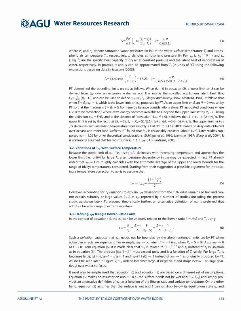
Figure 2. Variations of the Priestley-Taylor coefficient aPT across the sites labeled as Lakes with Lake L�eman in circle (o) and Lake Kinneretin plus (1), Reservoirs with the settling reservoir in greater than symbol (>) and the operational reservoir in less than symbol (<), andWetland in diamond (�) with (left) measured Bowen ratio b, (middle) measured surface temperature Ts, and (right) measured sensible heatflux H. The aavg predicted from equation (5) is shown in all the middle plots (dashed), and the relation between aPT and H derived overcrops as described elsewhere [Pereira and Villa-Nova, 1992] is also shown in the right plots (dash-dot). aPT 5 1.26 is also shown as athin-horizontal line.

Water Resources Research 10.1002/2015WR017504

ASSOULINE ET AL. THE PRIESTLEY-TAYLOR COEFFICIENT OVER WATER BODIES 156

Figure 2 (left) should not be interpreted as model-data comparisons. It simply highlights the ranges of aPT

and b covered at each of the sites.

Whether these aPT variations over water can be entirely explained by Ts changes as conjectured from equa-tion (5) or H as proposed by a previous study over crops [Pereira and Villa-Nova, 1992] is now considered.The relation between computed aPT values from equation (6) and Ts (middle) or H (right) for data corre-sponding to different water bodies is also presented in Figure 2. The horizontal thin line shows the widelyused aPT 5 1.26. It appears that there are no significant trends between measured aPT and Ts above watersurfaces. In several sites, and especially in the wetland, most of the aPT values are subunity. Figure 2 alsoshows variations in aavg computed from equation (5) with measured Ts (i.e., dashed lines in the middleplots), suggesting that surface temperature alone introduces large deviations from the accepted 1.26 value.In fact, the aavg variations in Figure 2 span a portion of the variations reported over water surfaces, althoughlarge scatter has already been reported in many studies depending on local conditions [Szilagyi et al., 2014].

Regarding the relation between aPT and H, this relation appears to be stronger than its Ts counterpart with aPT

decreasing as H increases. The shape of the aPT-H relation seems to depend on the nature of the water bodyand is clearly not universal. Lake L�eman and the wetland site do not follow a linear relation across the entirerange of measured H as found for Lake Kinneret and the Eshkol reservoirs. Evidently, measured H alone alsocannot explain the entire scatter in measured aPT between or across sites. However, aPT> 1.26 appears to beassociated with H< 0 while aPT< 1.26 appears to be associated with H> 0, with large scatter in aPT occurringwhen H � 0 both for Lake L�eman and the Tilopozo wetland. Interestingly, the general trend of aPT decreasingwith increasing H in Figure 2 is opposite to a linear increase in aPT with increasing H reported for crops [Pereiraand Villa-Nova, 1992]. What causes the difference in the aPT-H relation for free water surfaces and cropsremains unclear. Some studies over well-watered crops also suggest a trend consistent with the free watersurfaces here. For example, it was found by Jury and Tanner [1975] that for several well-irrigated crops, hori-zontal advection of dry air mass causes daily aPT to increase beyond its value inferred from measurements onnonadvective days as expected. The values of H inferred by us from the Jury and Tanner [1975] study suggestthat H< 0 during those advective conditions, which is in line with the free water surface data results here. Anempirical correction based on vapor pressure deficit to aPT in the aforementioned study appears to improvethe agreement between model calculations and lysimeter measurements of E. However, it is clear that the aPT

variations above water surfaces cannot be fully explained by Ts or H variations.

The prediction of aPT variations from routine meteorological measurements using the flux-variance methodis now discussed. Routine meteorological instruments for air temperature (e.g., thermocouples) and watervapor (e.g., hygrometers using electric capacitive elements) are slow-response instruments and are com-monly sampled at 0.1–1 Hz. Hence, prior to any discussion on aPT variability, it is necessary to assess howwell RwT=Rwq and RTq can be inferred from filtered and down-sampled time series. To do so, numericalexperiments are conducted on the 20 Hz (i.e., the highest sampling frequency across all experiments) tem-perature and water vapor series collected above Lake L�eman (in Switzerland), as a case study. To mimic vari-ous types of instrumentation filtering and subsampling and yet maintain some generality without imposing‘‘instrument specific’’ filtering, one-dimensional Gaussian and box filter functions are applied to the 20 Hzseries for conducting ‘‘low-pass’’ filtering (i.e., high frequencies filtered but low frequencies retained). The fil-tered series of some arbitrary flow variable S (i.e., w0; q0, or T 0), denoted as ~S, is computed from theconvolution

~S5

ð121

GðrÞS t2rð Þdr; (16)

where t denotes time and G(r) is a filter function. The Gaussian filter function is a Gaussian distribution withmean zero and variance set to ð1=12Þd2, where d is the cutoff frequency [Pope, 2000]. Similar filter functioncan be derived for box filtering as discussed elsewhere [Pope, 2000]. Figure 3 shows an example of how a20 Hz time series of w0; q0; and T 0 is filtered to 0.1 Hz using a one-dimensional Gaussian G(r). The examplein Figure 3 corresponds to the case with H 5 75 Wm22, E 5 217 W m22, aPT 5 0.74, and Ts518:1�C, whichyields RwT=Rwq 5 1.01, R~w ~T =R~w ~q 5 1.06, RTq 5 0.86, and R~T ~q 5 0.83.

Figure 4 shows comparisons between RwT=Rwq measured at 20 Hz against RwT=Rwq determined by applyinga Gaussian G(r) to w0; T 0, and q0. Three cutoff frequencies for G(r) are selected as 2, 1, and 0.1 Hz to illustrate

Water Resources Research 10.1002/2015WR017504

ASSOULINE ET AL. THE PRIESTLEY-TAYLOR COEFFICIENT OVER WATER BODIES 157

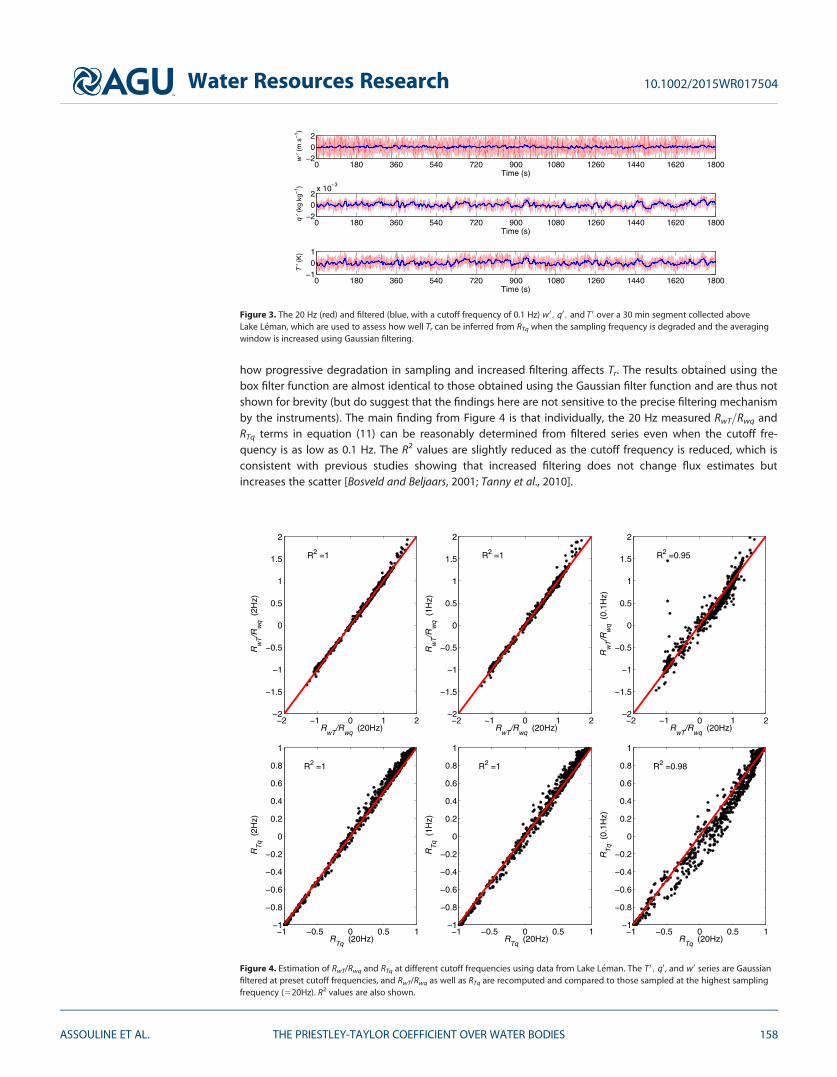
how progressive degradation in sampling and increased filtering affects Tr. The results obtained using thebox filter function are almost identical to those obtained using the Gaussian filter function and are thus notshown for brevity (but do suggest that the findings here are not sensitive to the precise filtering mechanismby the instruments). The main finding from Figure 4 is that individually, the 20 Hz measured RwT=Rwq andRTq terms in equation (11) can be reasonably determined from filtered series even when the cutoff fre-quency is as low as 0.1 Hz. The R2 values are slightly reduced as the cutoff frequency is reduced, which isconsistent with previous studies showing that increased filtering does not change flux estimates butincreases the scatter [Bosveld and Beljaars, 2001; Tanny et al., 2010].

−2 −1 0 1 2−2

−1.5

−1

−0.5

0

0.5

1

1.5

2

RwT

/Rwq

(20Hz)

Rw

T/R

wq (

2Hz)

R2 =1

−2 −1 0 1 2−2

−1.5

−1

−0.5

0

0.5

1

1.5

2

RwT

/Rwq

(20Hz)

Rw

T/R

wq (

1Hz)

R2 =1

−2 −1 0 1 2−2

−1.5

−1

−0.5

0

0.5

1

1.5

2

RwT

/Rwq

(20Hz)

Rw

T/R

wq (

0.1H

z)

R2 =0.95

−1 −0.5 0 0.5 1−1

−0.8

−0.6

−0.4

−0.2

0

0.2

0.4

0.6

0.8

1

RTq

(20Hz)

RT

q (2H

z)

R2 =1

−1 −0.5 0 0.5 1−1

−0.8

−0.6

−0.4

−0.2

0

0.2

0.4

0.6

0.8

1

RTq

(20Hz)

RT

q (1H

z)

R2 =1

−1 −0.5 0 0.5 1−1

−0.8

−0.6

−0.4

−0.2

0

0.2

0.4

0.6

0.8

1

RTq

(20Hz)

RT

q (0.

1Hz)

R2 =0.98

Figure 4. Estimation of RwT/Rwq and RTq at different cutoff frequencies using data from Lake L�eman. The T 0; q0 , and w0 series are Gaussianfiltered at preset cutoff frequencies, and RwT/Rwq as well as RTq are recomputed and compared to those sampled at the highest samplingfrequency (520Hz). R2 values are also shown.

0 180 360 540 720 900 1080 1260 1440 1620 1800−2

02

Time (s)

w ′

(m s

−1 )

0 180 360 540 720 900 1080 1260 1440 1620 1800−2

02

x 10−3

Time (s)

q ′

(kg

kg−

1 )

0 180 360 540 720 900 1080 1260 1440 1620 1800−1

01

Time (s) T

′ (K

)

Figure 3. The 20 Hz (red) and filtered (blue, with a cutoff frequency of 0.1 Hz) w0; q0; and T 0 over a 30 min segment collected aboveLake L�eman, which are used to assess how well Tr can be inferred from RTq when the sampling frequency is degraded and the averagingwindow is increased using Gaussian filtering.

Water Resources Research 10.1002/2015WR017504

ASSOULINE ET AL. THE PRIESTLEY-TAYLOR COEFFICIENT OVER WATER BODIES 158

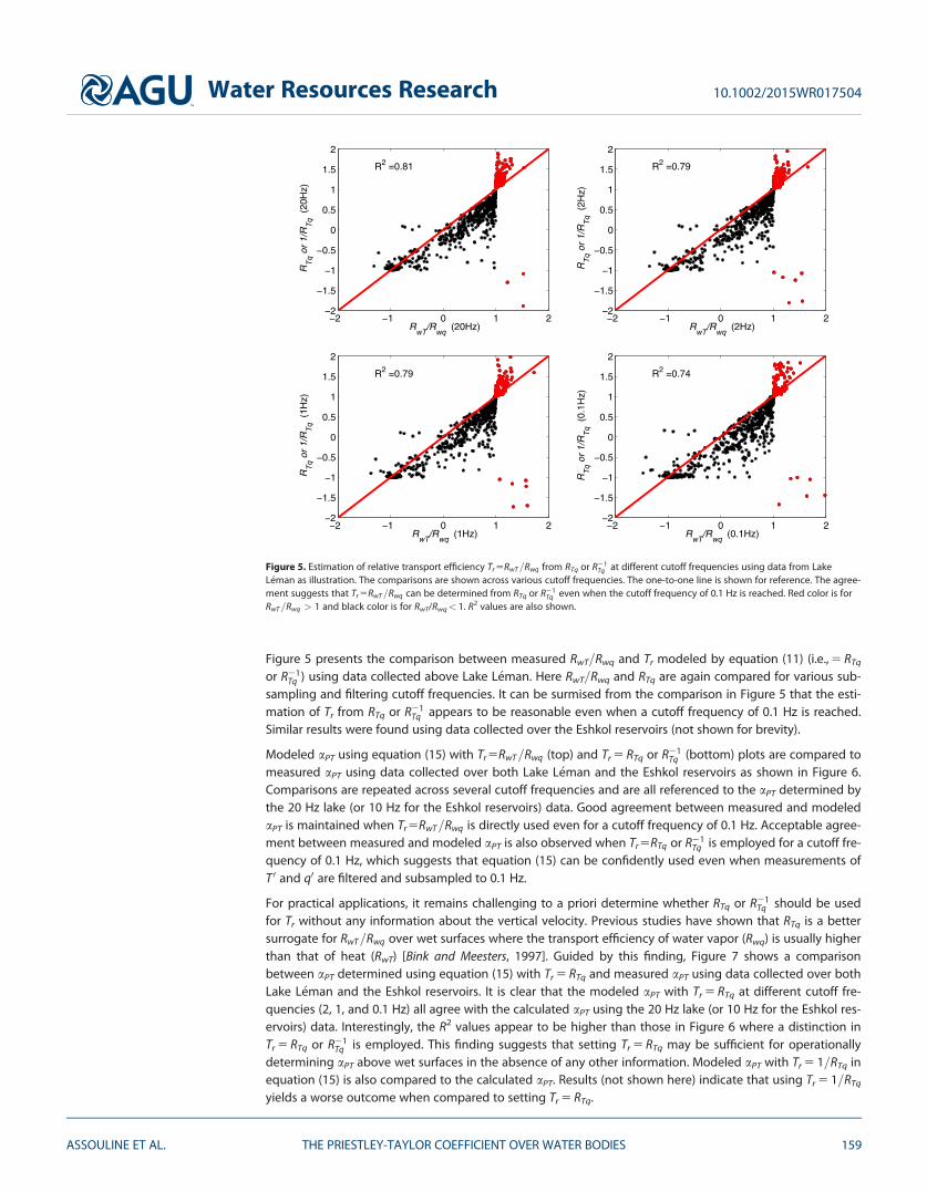
Figure 5 presents the comparison between measured RwT=Rwq and Tr modeled by equation (11) (i.e., 5 RTq

or R21Tq ) using data collected above Lake L�eman. Here RwT=Rwq and RTq are again compared for various sub-

sampling and filtering cutoff frequencies. It can be surmised from the comparison in Figure 5 that the esti-mation of Tr from RTq or R21

Tq appears to be reasonable even when a cutoff frequency of 0.1 Hz is reached.Similar results were found using data collected over the Eshkol reservoirs (not shown for brevity).

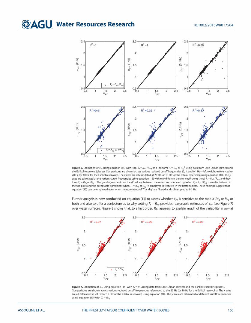
Modeled aPT using equation (15) with Tr5RwT=Rwq (top) and Tr 5 RTq or R21Tq (bottom) plots are compared to

measured aPT using data collected over both Lake L�eman and the Eshkol reservoirs as shown in Figure 6.Comparisons are repeated across several cutoff frequencies and are all referenced to the aPT determined bythe 20 Hz lake (or 10 Hz for the Eshkol reservoirs) data. Good agreement between measured and modeledaPT is maintained when Tr5RwT=Rwq is directly used even for a cutoff frequency of 0.1 Hz. Acceptable agree-ment between measured and modeled aPT is also observed when Tr5RTq or R21

Tq is employed for a cutoff fre-quency of 0.1 Hz, which suggests that equation (15) can be confidently used even when measurements ofT 0 and q0 are filtered and subsampled to 0.1 Hz.

For practical applications, it remains challenging to a priori determine whether RTq or R21Tq should be used

for Tr without any information about the vertical velocity. Previous studies have shown that RTq is a bettersurrogate for RwT=Rwq over wet surfaces where the transport efficiency of water vapor (Rwq) is usually higherthan that of heat (RwT) [Bink and Meesters, 1997]. Guided by this finding, Figure 7 shows a comparisonbetween aPT determined using equation (15) with Tr 5 RTq and measured aPT using data collected over bothLake L�eman and the Eshkol reservoirs. It is clear that the modeled aPT with Tr 5 RTq at different cutoff fre-quencies (2, 1, and 0.1 Hz) all agree with the calculated aPT using the 20 Hz lake (or 10 Hz for the Eshkol res-ervoirs) data. Interestingly, the R2 values appear to be higher than those in Figure 6 where a distinction inTr 5 RTq or R21

Tq is employed. This finding suggests that setting Tr 5 RTq may be sufficient for operationallydetermining aPT above wet surfaces in the absence of any other information. Modeled aPT with Tr 5 1=RTq inequation (15) is also compared to the calculated aPT. Results (not shown here) indicate that using Tr 5 1=RTq

yields a worse outcome when compared to setting Tr 5 RTq.

−2 −1 0 1 2−2

−1.5

−1

−0.5

0

0.5

1

1.5

2

RwT

/Rwq

(20Hz)

RT

q or

1/R

Tq (

20H

z)

R2 =0.81

−2 −1 0 1 2−2

−1.5

−1

−0.5

0

0.5

1

1.5

2

RwT

/Rwq

(2Hz)

RT

q or

1/R

Tq (

2Hz)

R2 =0.79

−2 −1 0 1 2−2

−1.5

−1

−0.5

0

0.5

1

1.5

2

RwT

/Rwq

(1Hz)

RT

q or

1/R

Tq (

1Hz)

R2 =0.79

−2 −1 0 1 2−2

−1.5

−1

−0.5

0

0.5

1

1.5

2

RwT

/Rwq

(0.1Hz)

RT

q or

1/R

Tq (

0.1H

z)

R2 =0.74

Figure 5. Estimation of relative transport efficiency Tr5RwT=Rwq from RTq or R21Tq at different cutoff frequencies using data from Lake

L�eman as illustration. The comparisons are shown across various cutoff frequencies. The one-to-one line is shown for reference. The agree-ment suggests that Tr 5RwT=Rwq can be determined from RTq or R21

Tq even when the cutoff frequency of 0.1 Hz is reached. Red color is forRwT=Rwq > 1 and black color is for RwT/Rwq< 1. R2 values are also shown.

Water Resources Research 10.1002/2015WR017504

ASSOULINE ET AL. THE PRIESTLEY-TAYLOR COEFFICIENT OVER WATER BODIES 159

Further analysis is now conducted on equation (15) to assess whether aPT is sensitive to the ratio rT/rq or RTq orboth and also to offer a conjecture as to why setting Tr 5 RTq provides reasonable estimates of aPT (see Figure 7)over water surfaces. Figure 8 shows that, to a first order, RTq appears to explain much of the variability in aPT (at

0.5 1 1.5 2 2.50.5

1

1.5

2

2.5

αPT

αP

T (

2Hz)

R2 =1

Tr = R

wT/R

wq

0.5 1 1.5 2 2.50.5

1

1.5

2

2.5

αPT

αP

T (

1Hz)

R2 =1

0.5 1 1.5 2 2.50.5

1

1.5

2

2.5

αPT

αP

T (

0.1H

z)

R2 =0.88

0.5 1 1.5 2 2.50.5

1

1.5

2

2.5

αPT

αP

T (

2Hz)

R2 =0.91

Tr = R

Tq or 1/R

Tq

0.5 1 1.5 2 2.50.5

1

1.5

2

2.5

αPT

αP

T (

1Hz)

R2 =0.92

0.5 1 1.5 2 2.50.5

1

1.5

2

2.5

αPT

αP

T (

0.1H

z)

R2 =0.87

Figure 6. Estimation of aPT using equation (15) with (top) Tr5RwT=Rwq and (bottom) Tr 5 RTq or R21Tq using data from Lake L�eman (circles) and

the Eshkol reservoirs (pluses). Comparisons are shown across various reduced cutoff frequencies (2, 1, and 0.1 Hz—left to right) referenced to20 Hz (or 10 Hz for the Eshkol reservoirs). The x axes are all calculated at 20 Hz (or 10 Hz for the Eshkol reservoirs) using equation (10). The yaxes are calculated at the various cutoff frequencies using equation (15) with two different transfer coefficients ((top) Tr5RwT=Rwq and (bot-tom) Tr 5 RTq or R21

Tq ). The good agreement (see the R2 values) between measured and modeled aPT when Tr5RwT=Rwq is used is featured inthe top plots and the acceptable agreement when Tr 5 RTq or R21

Tq is employed is featured in the bottom plots. These findings suggest thatequation (15) can be employed even when measurements of T 0 and q0 are filtered and subsampled to 0.1 Hz.

0.5 1 1.5 2 2.50.5

1

1.5

2

2.5

αPT

αP

T (

2Hz)

R2 =0.97

Tr = R

Tq

0.5 1 1.5 2 2.50.5

1

1.5

2

2.5

αPT

αP

T (

1Hz)

R2 =0.96

0.5 1 1.5 2 2.50.5

1

1.5

2

2.5

αPT

αP

T (

0.1H

z)

R2 =0.95

Figure 7. Estimation of aPT using equation (15) with Tr 5 RTq using data from Lake L�eman (circles) and the Eshkol reservoirs (pluses).Comparisons are shown across various reduced cutoff frequencies referenced to the 20 Hz (or 10 Hz for the Eshkol reservoirs). The x axesare all calculated at 20 Hz (or 10 Hz for the Eshkol reservoirs) using equation (10). The y axes are calculated at different cutoff frequenciesusing equation (15) with Tr 5 RTq.

Water Resources Research 10.1002/2015WR017504

ASSOULINE ET AL. THE PRIESTLEY-TAYLOR COEFFICIENT OVER WATER BODIES 160

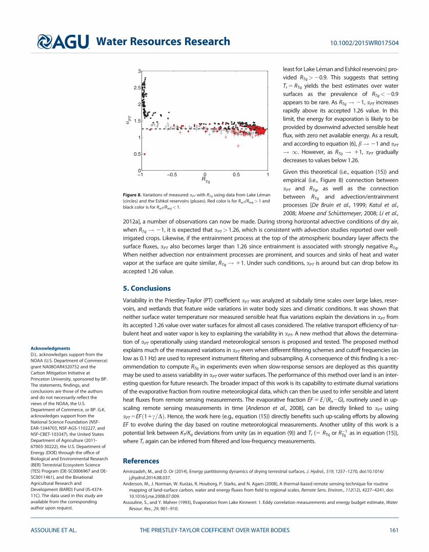
least for Lake L�eman and Eshkol reservoirs) pro-vided RTq>20.9. This suggests that settingTr 5 RTq yields the best estimates over watersurfaces as the prevalence of RTq<20.9appears to be rare. As RTq! 21, aPT increasesrapidly above its accepted 1.26 value. In thislimit, the energy for evaporation is likely to beprovided by downwind advected sensible heatflux, with zero net available energy. As a result,and according to equation (6), b!21 and aPT

! 1. However, as RTq ! 11, aPT graduallydecreases to values below 1.26.

Given this theoretical (i.e., equation (15)) andempirical (i.e., Figure 8) connection betweenaPT and RTq, as well as the connectionbetween RTq and advection/entrainmentprocesses [De Bruin et al., 1999; Katul et al.,2008; Moene and Sch€uttemeyer, 2008; Li et al.,

2012a], a number of observations can now be made. During strong horizontal advective conditions of dry air,when RTq! 21, it is expected that aPT> 1.26, which is consistent with advection studies reported over well-irrigated crops. Likewise, if the entrainment process at the top of the atmospheric boundary layer affects thesurface fluxes, aPT also becomes larger than 1.26 since entrainment is associated with strongly negative RTq.When neither advection nor entrainment processes are prominent, and sources and sinks of heat and watervapor at the surface are quite similar, RTq! 11. Under such conditions, aPT is around but can drop below itsaccepted 1.26 value.

5. Conclusions

Variability in the Priestley-Taylor (PT) coefficient aPT was analyzed at subdaily time scales over large lakes, reser-voirs, and wetlands that feature wide variations in water body sizes and climatic conditions. It was shown thatneither surface water temperature nor measured sensible heat flux variations explain the deviations in aPT fromits accepted 1.26 value over water surfaces for almost all cases considered. The relative transport efficiency of tur-bulent heat and water vapor is key to explaining the variability in aPT. A new method that allows the determina-tion of aPT operationally using standard meteorological sensors is proposed and tested. The proposed methodexplains much of the measured variations in aPT even when different filtering schemes and cutoff frequencies (aslow as 0.1 Hz) are used to represent instrument filtering and subsampling. A consequence of this finding is a rec-ommendation to compute RTq in experiments even when slow-response sensors are deployed as this quantitymay be used to assess variability in aPT over water surfaces. The performance of this method over land is an inter-esting question for future research. The broader impact of this work is its capability to estimate diurnal variationsof the evaporative fraction from routine meteorological data, which can then be used to infer sensible and latentheat fluxes from remote sensing measurements. The evaporative fraction EF 5 E=(Rn2G), routinely used in up-scaling remote sensing measurements in time [Anderson et al., 2008], can be directly linked to aPT usingaPT 5EFð11c=DÞ. Hence, the work here (e.g., equation (15)) directly benefits such up-scaling efforts by allowingEF to evolve during the day based on routine meteorological measurements. Another utility of this work is apotential link between KT/Kq deviations from unity (as in equation (9)) and Tr (5 RTq or R21

Tq as in equation (15)),where Tr again can be inferred from filtered and low-frequency measurements.

ReferencesAminzadeh, M., and D. Or (2014), Energy partitioning dynamics of drying terrestrial surfaces, J. Hydrol., 519, 1257–1270, doi:10.1016/

j.jhydrol.2014.08.037.Anderson, M., J. Norman, W. Kustas, R. Houborg, P. Starks, and N. Agam (2008), A thermal-based remote sensing technique for routine

mapping of land-surface carbon, water and energy fluxes from field to regional scales, Remote Sens. Environ., 112(12), 4227–4241, doi:10.1016/j.rse.2008.07.009.

Assouline, S., and Y. Mahrer (1993), Evaporation from Lake Kinneret: 1. Eddy correlation measurements and energy budget estimate, WaterResour. Res., 29, 901–910.

−1 −0.5 0 0.5 10

0.5

1

1.5

2

2.5

3

RTq

αP

T

Figure 8. Variations of measured aPT with RTq using data from Lake L�eman(circles) and the Eshkol reservoirs (pluses). Red color is for RwT/Rwq> 1 andblack color is for RwT/Rwq< 1.

AcknowledgmentsD.L. acknowledges support from theNOAA (U.S. Department of Commerce)grant NA08OAR4320752 and theCarbon Mitigation Initiative atPrinceton University, sponsored by BP.The statements, findings, andconclusions are those of the authorsand do not necessarily reflect theviews of the NOAA, the U.S.Department of Commerce, or BP. G.K.acknowledges support from theNational Science Foundation (NSF-EAR-1344703, NSF-AGS-1102227, andNSF-CBET-103347), the United StatesDepartment of Agriculture (2011-67003-30222), the U.S. Department ofEnergy (DOE) through the office ofBiological and Environmental Research(BER) Terrestrial Ecosystem Science(TES) Program (DE-SC0006967 and DE-SC0011461), and the BinationalAgricultural Research andDevelopment (BARD) Fund (IS-4374-11C). The data used in this study areavailable from the correspondingauthor upon request.

Water Resources Research 10.1002/2015WR017504

ASSOULINE ET AL. THE PRIESTLEY-TAYLOR COEFFICIENT OVER WATER BODIES 161

Assouline, S., S. Tyler, J. Tanny, S. Cohen, E. Bou-Zeid, M. Parlange, and G. Katul (2008), Evaporation from three water bodies of differentsizes and climates: Measurements and scaling analysis, Adv. Water Resour., 31(1), 160–172, doi:10.1016/j.advwatres.2007.07.003.

Bates, G. T., S. W. Hostetler, and F. Giorgi (1995), Two-year simulation of the great lakes region with a coupled modeling system, Mon.Weather Rev., 123(5), 1505–1522.

Bink, N., and A. Meesters (1997), Comment on estimation of surface heat and momentum fluxes using the flux-variance method above uni-form and non-uniform terrain by Katul et al. (1995), Boundary Layer Meteorol., 84(3), 497–502.

Blanken, P. D., W. R. Rouse, A. D. Culf, C. Spence, L. D. Boudreau, J. N. Jasper, B. Kochtubajda, W. M. Schertzer, P. Marsh, and D. Verseghy (2000),Eddy covariance measurements of evaporation from great slave lake, northwest territories, Canada, Water Resour. Res., 36, 1069–1077.

Blanken, P. D., W. R. Rouse, and W. M. Schertzer (2003), Enhancement of evaporation from a large northern lake by the entrainment ofwarm, dry air, J. Hydrometeorol., 4(4), 680–693.

Blanken, P. D., C. Spence, N. Hedstrom, and J. D. Lenters (2011), Evaporation from lake superior: 1. Physical controls and processes, J. GreatLakes Res., 37(4), 707–716.

Bosveld, F. C., and A. C. Beljaars (2001), The impact of sampling rate on eddy-covariance flux estimates, Agric. For. Meteorol., 109(1), 39–45.Bou-Zeid, E., N. Vercauteren, M. B. Parlange, and C. Meneveau (2008), Scale dependence of subgrid-scale model coefficients: An a priori

study, Phys. Fluids, 20(11), 115–106.Brutsaert, W. (2005), Hydrology: An Introduction, Cambridge Univ. Press, N. Y.Brutsaert, W., and H. Stricker (1979), An advection-aridity approach to estimate actual regional evapotranspiration, Water Resour. Res., 15,

443–450, doi:10.1029/WR015i002p00443.Chen, D., and W. Brutsaert (1995), Diagnostics of land surface spatial variability and water vapor flux, J. Geophys. Res., 100, 25,595–25,606,

doi:10.1029/95JD00973.Cho, J., T. Oki, P.-F. Yeh, W. Kim, S. Kanae, and K. Otsuki (2012), On the relationship between the Bowen ratio and the near-surface air tem-

perature, Theor. Appl. Climatol., 108(1–2), 135–145, doi:10.1007/s00704-011-0520-y.Courant, R., and D. Hilbert (1953), Methods of Mathematical Physics, vol.1, John Wiley, N. Y.Crago, R., and R. Crowley (2005), Complementary relationships for near-instantaneous evaporation, J. Hydrol., 300, 199–211, doi:10.1016/

j.jhydrol.2004.06.002.Crago, R. D. (1996), Comparison of the evaporative fraction and the Priestley-Taylor a for parameterizing daytime evaporation, Water

Resour. Res., 32, 1403–1409.Culf, A. (1994), Equilibrium evaporation beneath a growing convective boundary layer, Boundary Layer Meteorol., 70(1-2), 37–49, doi:

10.1007/BF00712522.Davis, J., and C. Allen (1973), Equilibrium, potential and actual evaporation from cropped surfaces in southern Ontario, J. Appl. Meteorol.,

12, 649–657.De Bruin, H. (1983), A model of the Priestley-Taylor parameter a, J. Clim. Appl. Meteorol., 22, 572–578.De Bruin, H., and J. Keijman (1979), The Priestley-Taylor evaporation model applied to a large, shallow lake in the Netherlands, J. Appl. Mete-

orol., 18, 898–903.De Bruin, H., B. Van Den Hurk, and L. Kroon (1999), On the temperature-humidity correlation and similarity, Boundary Layer Meteorol., 93(3),

453–468.Eichinger, W. E., M. B. Parlange, and H. Stricker (1996), On the concept of equilibrium evaporation and the value of the Priestley-Taylor coef-

ficient, Water Resour. Res., 32, 161–164, doi:10.1029/95WR02920.Flint, A. L., and S. W. Childs (1991), Use of the Priestley-Taylor evaporation equation for soil water limited conditions in a small forest clear-

cut, Agric. For. Meteorol., 56, 247–260, doi:10.1016/0168-1923(91)90094-7.Granger, R. (1989), A complementary relationship approach for evaporation from nonsaturated surfaces, J. Hydrol., 111(1–4), 31–38, doi:

10.1016/0022-1694(89)90250-3.Granger, R., and D. Gray (1989), Evaporation from natural nonsaturated surfaces, J. Hydrol., 111(1–4), 21–29, doi:10.1016/0022-

1694(89)90249-7.Granger, R., and N. Hedstrom (2011), Modelling hourly rates of evaporation from small lakes, Hydrol. Earth Syst. Sci., 15(1), 267–277.Guo, X., H. Liu, and K. Yang (2015), On the application of the Priestley–Taylor relation on sub-daily time scales, Boundary Layer Meteorol.,

156, 489–499.Huntingford, C., and J. Monteith (1998), The behaviour of a mixed-layer model of the convective boundary layer coupled to a big leaf

model of surface energy partitioning, Boundary Layer Meteorol., 88(1), 87–101.Jarvis, P. G., and K. McNaughton (1986), Stomatal control of transpiration: Scaling up from leaf to region, Adv. Ecol. Res., 15, 1–49.Jonsson, A., J. Åberg, A. Lindroth, and M. Jansson (2008), Gas transfer rate and CO2 flux between an unproductive lake and the atmosphere

in northern Sweden, J. Geophys. Res., 113, G04006, doi:10.1029/2008JG000688.Jury, W., and C. Tanner (1975), Advection modification of the Priestley and Taylor evapotranspiration formula, Agron. J., 67, 840–842, doi:

10.2134/agronj1975.00021962006700060031x.Katul, G., and C.-I. Hsieh (1997), Reply to the comment by bink and meesters, Boundary Layer Meteorol., 84(3), 503–509.Katul, G. G., and C.-I. Hsieh (1999), A note on the flux-variance similarity relationships for heat and water vapour in the unstable atmos-

pheric surface layer, Boundary Layer Meteorol., 90(2), 327–338.Katul, G. G., and M. B. Parlange (1992), A Penman-Brutsaert model for wet surface evaporation, Water Resour. Res., 28, 121–126, doi:

10.1029/91WR02324.Katul, G. G., A. M. Sempreviva, and D. Cava (2008), The temperature–humidity covariance in the marine surface layer: A one-dimensional

analytical model, Boundary Layer Meteorol., 126(2), 263–278.Komatsu, H. (2005), Forest categorization according to dry-canopy evaporation rates in the growing season: Comparison of the Priestley–

Taylor coefficient values from various observation sites, Hydrol. Processes, 19(19), 3873–3896.Lamaud, E., and M. Irvine (2006), Temperature–humidity dissimilarity and heat-to-water-vapour transport efficiency above and within a

pine forest canopy: The role of the Bowen ratio, Boundary Layer Meteorol., 120(1), 87–109.Lhomme, J.-P. (1997), A theoretical basis for the Priestley-Taylor coefficient, Boundary Layer Meteorol., 82(2), 179–191, doi:10.1023/A:

1000281114105.Li, D., and E. Bou-Zeid (2011), Coherent structures and the dissimilarity of turbulent transport of momentum and scalars in the unstable

atmospheric surface layer, Boundary Layer Meteorol., 140(2), 243–262.Li, D., E. Bou-Zeid, and H. de Bruin (2012a), Monin-Obukhov similarity functions for the structure parameters of temperature and humidity,

Boundary Layer Meteorol., 145(1), 45–67.

Water Resources Research 10.1002/2015WR017504

ASSOULINE ET AL. THE PRIESTLEY-TAYLOR COEFFICIENT OVER WATER BODIES 162

Li, D., G. Katul, and E. Bou-Zeid (2012b), Mean velocity and temperature profiles in a sheared diabatic turbulent boundary layer, Phys. Fluids,24(10), 105105.

Li, D., G. G. Katul, and E. Bou-Zeid (2015), Turbulent energy spectra and cospectra of momentum and heat fluxes in the stable atmosphericsurface layer, Boundary Layer Meteorol., 157, 1–21.

Liu, H., Y. Zhang, S. Liu, H. Jiang, L. Sheng, and Q. L. Williams (2009), Eddy covariance measurements of surface energy budget and evapora-tion in a cool season over southern open water in Mississippi, J. Geophys. Res., 114, D04110, doi:10.1029/2008JD010891.

McNaughton, K., and P. Jarvis (1991), Effects of spatial scale on stomatal control of transpiration, Agric. For. Meteorol., 54(2), 279–302.McNaughton, K., and T. Spriggs (1986), A mixed-layer model for regional evaporation, Boundary Layer Meteorol., 34(3), 243–262.Moene, A. F., and D. Sch€uttemeyer (2008), The effect of surface heterogeneity on the temperature–humidity correlation and the relative

transport efficiency, Boundary Layer Meteorol., 129(1), 99–113.Monteith, J. (1995), A reinterpretation of stomatal responses to humidity, Plant Cell Environ., 18(4), 357–364.Monteith, J. L. (1981), Evaporation and surface temperature, Q. J. R. Meteorol. Soc., 107(451), 1–27, doi:10.1002/qj.49710745102.Nordbo, A., S. Launiainen, I. Mammarella, M. Lepp€aranta, J. Huotari, A. Ojala, and T. Vesala (2011), Long-term energy flux measurements and

energy balance over a small boreal lake using eddy covariance technique, J. Geophys. Res., 116, D02119, doi:10.1029/2010JD014542.Nullet, D., and T. W. Giambelluca (1990), Winter evaporation on a mountain slope, Hawaii, J. Hydrol., 112(3), 257–265.Panin, G. N., A. Nasonov, T. Foken, and H. Lohse (2006), On the parameterisation of evaporation and sensible heat exchange for shallow

lakes, Theor. Appl. Climatol., 85(3-4), 123–129.Parlange, M. B., and G. G. Katul (1992a), An advection-aridity evaporation model, Water Resour. Res., 28, 127–132, doi:10.1029/91WR02482.Parlange, M. B., and G. G. Katul (1992b), Estimation of the diurnal variation of potential evaporation from a wet bare soil surface, J. Hydrol.,

132(1), 71–89.Penman, H. L. (1948), Natural evaporation from open water, bare soil and grass, Proc. R. Soc. London, Ser. A, 193(1032), 120–145, doi:

10.1098/rspa.1948.0037.Pereira, A. R. (2004), The Priestley-Taylor parameter and the decoupling factor for estimating reference evapotranspiration, Agric. For. Mete-

orol., 125, 305–313, doi:10.1016/j.agrformet.2004.04.002.Pereira, A. R., and N. A. Villa-Nova (1992), Analysis of the Priestley-Taylor parameter, Agric. For. Meteorol., 61, 1–9, doi:10.1016/0168-

1923(92)90021-U.Pope, S. (2000), Turbulent Flows, 771 pp., Cambridge Univ. Press, Cambridge, U. K.Priestley, C., and R. Taylor (1972), On the assessment of surface heat flux and evaporation, Mon. Weather Rev., 106, 81–92.Rouse, W. R., P. D. Blanken, N. Bussieres, A. E. Walker, C. J. Oswald, W. M. Schertzer, and C. Spence (2008), An investigation of the thermal

and energy balance regimes of great slave and great bear lakes, J. Hydrometeorol., 9(6), 1318–1333.Slatyer, R., and I. McIlroy (1967), Practical Microclimatology, Commonw. Sci. Ind. Res. Organ., Melbourne, Australia.Spittlehouse, D. L., and T. A. Black (1981), A growing season water balance model applied to two douglas fir stands, Water Resour. Res., 17,

1651–1656, doi:10.1029/WR017i006p01651.Stannard, D. I. (1993), Comparison of Penman-Monteith, Shuttleworth-Wallace, and modified Priestley-Taylor evapotranspiration models

for wildland vegetation in semiarid rangeland, Water Resour. Res., 29, 1379–1392.Stannard, D. I., and D. O. Rosenberry (1991), A comparison of short-term measurements of lake evaporation using eddy correlation and

energy budget methods, J. Hydrol., 122(1), 15–22, doi:10.1016/0022-1694(91)90168-H.Stull, R. (1988), An Introduction to Boundary Layer Meteorology, Kluwer Acad., Dordrecht, Netherlands.Sumner, D. M., and J. M. Jacobs (2005), Utility of Penman–Monteith, Priestley–Taylor, reference evapotranspiration, and pan evaporation

methods to estimate pasture evapotranspiration, J. Hydrol., 308(1), 81–104.Szilagyi, J. (2014), Temperature corrections in the Priestley and Taylor equation of evaporation, J. Hydrol., 519, 455–464, doi:10.1016/

j.jhydrol.2014.07.040.Szilagyi, J., and J. Jozsa (2008), New findings about the complementary relationship-based evaporation estimation methods, J. Hydrol., 354,

171–186, doi:10.1016/j.jhydrol.2008.03.008.Szilagyi, J., and A. Schepers (2014), Coupled heat and vapor transport: The thermostat effect of a freely evaporating land surface, Geophys.

Res. Lett., 41, 435–441, doi:10.1002/2013GL058979.Szilagyi, J., M. T. Hobbins, and J. Jozsa (2009), Modified advection-aridity model of evapotranspiration, J. Hydrol. Eng., 14(6), 569–574.Szilagyi, J., M. B. Parlange, and G. G. Katul (2014), Assessment of the Priestley-Taylor parameter value from era-interim global reanalysis

data, J. Hydrol. Environ. Res., 2(1), 1–7.Tanner, B., and J. Greene (1989), Measurement of Sensible Heat and Water Vapor Fluxes Using Eddy Correlation Methods, Campbell Sci. Inc.,

Logan, Utah.Tanny, J., S. Cohen, S. Assouline, F. Lange, A. Grava, D. Berger, B. Teltch, and M. Parlange (2008), Evaporation from a small water reservoir:

Direct measurements and estimates, J. Hydrol., 351(1), 218–229, doi:10.1016/j.jhydrol.2007.12.012.Tanny, J., U. Dicken, and S. Cohen (2010), Vertical variation in turbulence statistics and energy balance in a banana screenhouse, Biosyst.

Eng., 106(2), 175–187.Tanny, J., S. Cohen, D. Berger, B. Teltch, Y. Mekhmandarov, M. Bahar, G. Katul, and S. Assouline (2011), Evaporation from a reservoir with

fluctuating water level: Correcting for limited fetch, J. Hydrol., 404, 146–156, doi:10.1016/j.jhydrol.2011.04.025.Venturini, V., S. Islam, and L. Rodriguez (2008), Estimation of evaporative fraction and evapotranspiration from MODIS products using a

complementary based model, Remote Sens. Environ., 112(1), 132–141, doi:10.1016/j.rse.2007.04.014.Vercauteren, N., E. Bou-Zeid, M. Parlange, U. Lemmin, H. Huwald, J. Selker, and C. Meneveau (2008), Subgrid-scale dynamics of water

vapour, heat, and momentum over a lake, Boundary Layer Meteorol., 128(2), 205–228, doi:10.1007/s10546-008-9287-9.Viswanadham, Y., V. S. Filho, and R. Andre (1991), The Priestley-Taylor parameter a for the amazon forest, For. Ecol. Manage., 38(3), 211–

225, doi:10.1016/0378-1127(91)90143-J.Wang, J., G. D. Salvucci, and R. L. Bras (2004), An extremum principle of evaporation, Water Resour. Res., 40, W09303, doi:10.1029/

2004WR003087.Yang, H., D. Yang, and Z. Lei (2013), Seasonal variability of the complementary relationship in the Asian monsoon region, Hydrol. Processes,

27(19), 2736–2741, doi:10.1002/hyp.9400.Yu, T. (1977), Parameterization of surface evaporation rate for use in numerical modeling, J. Appl. Meteorol., 16, 393–400.

Water Resources Research 10.1002/2015WR017504

ASSOULINE ET AL. THE PRIESTLEY-TAYLOR COEFFICIENT OVER WATER BODIES 163