On the Use of Numeraires in Option Pricing IT IS ILLEGAL ...rolf/teaching/PhDcourse/BBWnumeraire.pdf · On the Use of Numeraires in Option Pricing SIMON BENNINGA, TOMAS BJÖRK, AND

IT IS

ILLE

GAL

TO R

EPRODUCE T

HIS A

RTICLE

IN A

NY FO

RMAT

WINTER 2002 THE JOURNAL OF DERIVATIVES 43

Significant computational simplification is achievedwhen option pricing is approached through the changeof numeraire technique. By pricing an asset in termsof another traded asset (the numeraire), this techniquereduces the number of sources of risk that need to beaccounted for. The technique is useful in pricing com-plicated derivatives.

This article discusses the underlying theory of thenumeraire technique, and illustrates it with fivepricing problems: pricing savings plans that offer achoice of interest rates; pricing convertible bonds;pricing employee stock ownership plans; pricingoptions whose strike price is in a currency differentfrom the stock price; and pricing options whose strikeprice is correlated with the short-term interest rate.

While the numeraire method iswell-known in the theoreticalliterature, it appears to beinfrequently used in more

applied research, and many practitioners seemunaware of how to use it as well as when it isprofitable (or not) to use it. To illustrate the uses(and possible misuses) of the method, we dis-cuss in some detail five concrete applied prob-lems in option pricing:

• Pricing employee stock ownership plans.• Pricing options whose strike price is in

a currency different from the stock price.• Pricing convertible bonds.• Pricing savings plans that provide a choice

of indexing.

• Pricing options whose strike price is cor-related with the short-term interest rate.

The standard Black-Scholes (BS) formulaprices a European option on an asset that fol-lows geometric Brownian motion. The asset’suncertainty is the only risk factor in the model.A more general approach developed by Black-Merton-Scholes leads to a partial differentialequation. The most general method devel-oped so far for the pricing of contingent claimsis the martingale approach to arbitrage theorydeveloped by Harrison and Kreps [1981], Har-rison and Pliska [1981], and others.

Whether one uses the PDE or the stan-dard risk-neutral valuation formulas of themartingale method, it is in most cases veryhard to obtain analytic pricing formulas. Thus,for many important cases, special formulas(typically modifications of the original BS for-mula) have been developed. See Haug [1997]for extensive examples.

One of the most typical cases with mul-tiple risk factors occurs when an option involvesa choice between two assets with stochasticprices. In this case, it is often of considerableadvantage to use a change of numeraire in thepricing of the option. We show where thenumeraire approach leads to significant sim-plifications, but also where the numeraire changeis trivial, or where an obvious numeraire changereally does not simplify the computations.

On the Use of Numeraires in Option PricingSIMON BENNINGA, TOMAS BJÖRK, AND ZVI WIENER

SIMON BENNINGA

is a professor of finance at Tel-Aviv University in [email protected]

TOMAS BJÖRK

is a professor of mathe-matical finance at theStockholm School of Economics in [email protected]

ZVI WIENER

is a senior lecturer infinance at the School of Business at the HebrewUniversity of Jerusalem in [email protected]

Copyright © 2002 Institutional Investor, Inc. All Rights Reserved

The main message is that in many cases the changeof numeraire approach leads to a drastic simplification inthe computations. For each of five different option pricingproblems, we present the possible choices of numeraire,discuss the pros and cons of the various numeraires, andcompute the option prices.

I. CHANGE OF NUMERAIRE APPROACH

The basic idea of the numeraire approach can bedescribed as follows. Suppose that an option’s pricedepends on several (say, n) sources of risk. We may thencompute the price of the option according to this scheme:

• Pick a security that embodies one of the sources ofrisk, and choose this security as the numeraire.

• Express all prices in the market, including that of theoption, in terms of the chosen numeraire. In otherwords, perform all the computations in a relativeprice system.

• Since the numeraire asset in the new price system isriskless (by definition), we have reduced the numberof risk factors by one, from n to n – 1. If, for example,we start out with two sources of risk, eliminatingone may allow us to apply standard one-risk factoroption pricing formulas (such as Black-Scholes).

• We thus derive the option price in terms of thenumeraire. A simple translation from the numeraireback to the local currency will then give the priceof the option in monetary terms.

The standard numeraire reference in an abstract set-ting is Geman, El Karoui, and Rochet [1995]. We firstconsider a Markovian framework that is simpler thantheirs, but that is still reasonably general. All details andproofs can be found in Björk [1999].1

Assumption 1. Given a priori are:

• An empirically observable (k + 1)-dimensionalstochastic process:

X = (X1, …, Xk + 1)

with the notational convention that the process k + 1 isthe riskless rate:

Xk + 1(t) = r(t)

• We assume that under a fixed risk-neutral martin-gale measure Q the factor dynamics have the form:

dXi(t) = µi(t, X(t))dt + δi(t, X(t))dW(t)i = 1, …, k + 1

where W = (W1, …, Wd)´ is a standard d-dimensionalQ-Wiener process and δi = (δi1, δi2, …, δid) is a row vector.The superscript ´ denotes transpose.

• A risk-free asset (money account) with the dynamics:

dB(t) = r(t)B(t)dt

The interpretation is that the components of thevector process X are the underlying factors in the economy.

44 ON THE USE OF NUMERAIRES IN OPTION PRICING WINTER 2002

THE HISTORY OF THE NUMERAIRE APPROACHIN OPTION PRICING

The idea of using a numeraire to simplify optionpricing seems to have a history almost as long as theBlack-Scholes formula—a formula that might itself beinterpreted as using the dollar as a numeraire. In 1973,the year the Black-Scholes paper was published,Merton [1973] used a change of numeraire (thoughwithout using the name) to derive the value of a Euro-pean call (in units of zero coupon bond) with astochastic yield on the zero. Margrabe’s 1978 paper inthe Journal of Finance on exchange options was the firstto give the numeraire idea wide press. Margrabe appearsalso to have primacy in using the “numeraire” nomen-clature. In his paper Margrabe acknowledges a sug-gestion from Steve Ross, who had suggested that usingone of the assets as a numeraire would reduce theproblem to the Black-Scholes solution and obviate anyfurther mathematics.

In the same year that Margrabe’s paper was pub-lished, two other papers, Brenner-Galai [1978] andFischer [1978], made use of an approach which wouldnow be called the numeraire approach. In the fol-lowing year Harrison-Kreps [1979, p. 401] used theprice of a security with a strictly positive price asnumeraire. Hence, their numeraire asset has no marketrisk and pays an interest rate that equals zero, which isconvenient for their analysis. In 1989 papers by Geman[1989] and Jamshidian [1989] formalized the mathe-matics behind the numeraire approach.

It is illegal to reproduce this article in any format. Email [email protected] for Reprints or Permissions.

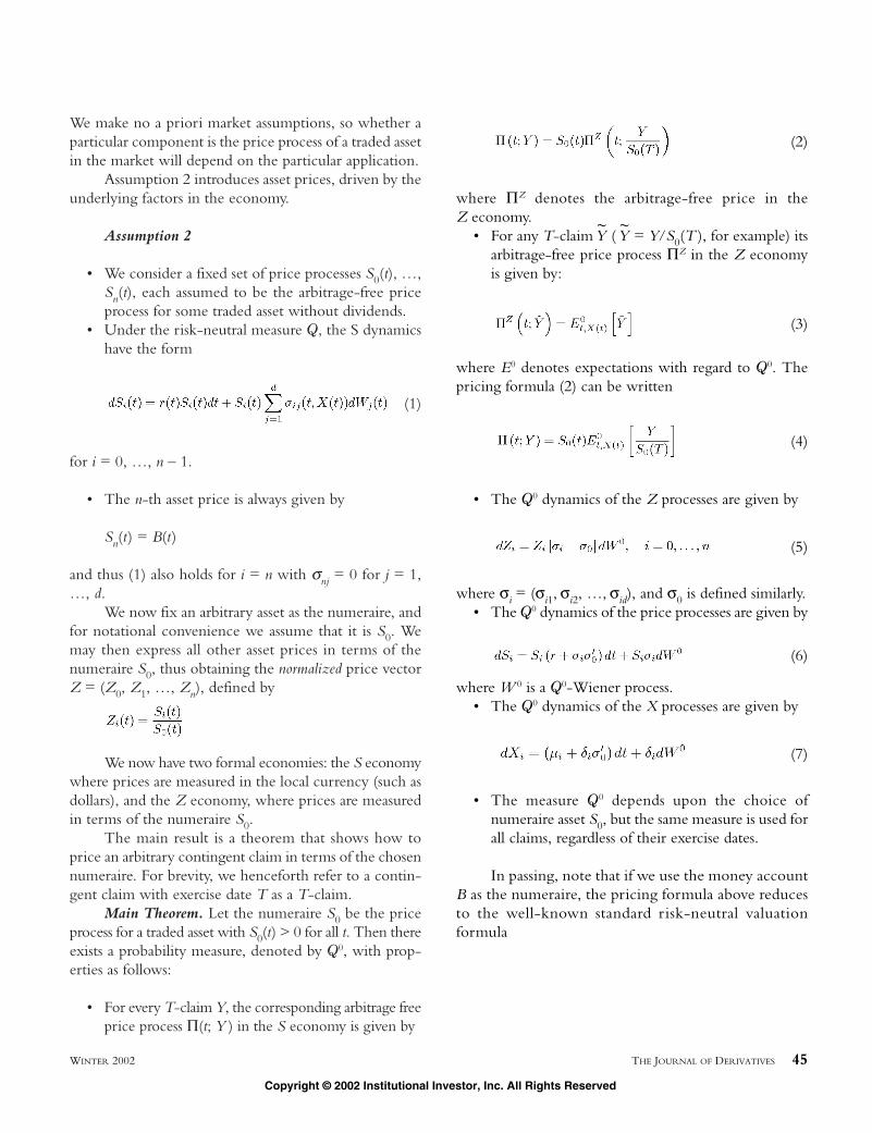
We make no a priori market assumptions, so whether aparticular component is the price process of a traded assetin the market will depend on the particular application.

Assumption 2 introduces asset prices, driven by theunderlying factors in the economy.

Assumption 2

• We consider a fixed set of price processes S0(t), …,Sn(t), each assumed to be the arbitrage-free priceprocess for some traded asset without dividends.

• Under the risk-neutral measure Q, the S dynamicshave the form

(1)

for i = 0, …, n – 1.

• The n-th asset price is always given by

Sn(t) = B(t)

and thus (1) also holds for i = n with σnj = 0 for j = 1,…, d.

We now fix an arbitrary asset as the numeraire, andfor notational convenience we assume that it is S0. Wemay then express all other asset prices in terms of thenumeraire S0, thus obtaining the normalized price vectorZ = (Z0, Z1, …, Zn), defined by

We now have two formal economies: the S economywhere prices are measured in the local currency (such asdollars), and the Z economy, where prices are measuredin terms of the numeraire S0.

The main result is a theorem that shows how toprice an arbitrary contingent claim in terms of the chosennumeraire. For brevity, we henceforth refer to a contin-gent claim with exercise date T as a T-claim.

Main Theorem. Let the numeraire S0 be the priceprocess for a traded asset with S0(t) > 0 for all t. Then thereexists a probability measure, denoted by Q0, with prop-erties as follows:

• For every T-claim Y, the corresponding arbitrage freeprice process Π(t; Y ) in the S economy is given by

(2)

where ΠZ denotes the arbitrage-free price in the Z economy.

• For any T-claim ~Y (

~Y = Y/S0(T ), for example) its

arbitrage-free price process ΠZ in the Z economyis given by:

(3)

where E0 denotes expectations with regard to Q0. Thepricing formula (2) can be written

(4)

• The Q0 dynamics of the Z processes are given by

(5)

where σi = (σi1, σi2, …, σid), and σ0 is defined similarly.• The Q0 dynamics of the price processes are given by

(6)

where W 0 is a Q0-Wiener process.• The Q0 dynamics of the X processes are given by

(7)

• The measure Q0 depends upon the choice ofnumeraire asset S0, but the same measure is used forall claims, regardless of their exercise dates.

In passing, note that if we use the money accountB as the numeraire, the pricing formula above reducesto the well-known standard risk-neutral valuation formula



(8)

In more pedestrian terms, the main points of theTheorem above are as follows:

• Equation (2) shows that the measure Q0 takes care ofthe stochasticity related to the numeraire S0. Note thatwe do not have to compute the price S0(t)—we simplyuse the observed market price.

We also see that if the claim Y is of the form Y =Y0S0(T ) (where Y0 is some T-claim) then the changeof numeraire is a huge simplification of the standardrisk-neutral formula (8). Instead of computing thejoint distribution of ∫Ttr(s)ds and Y (under Q), we haveonly to compute the distribution of Y0 (under Q0).

• Equation (3) shows that in the Z economy, prices arecomputed as expected values of the claim. Observethat there is no discounting factor in (3). The reasonis that in the Z economy, the price process Z0 has theproperty that Z0(t) = 1 for all t. Thus, in the Zeconomy there is a riskless asset with unit price. Thatis, in the Z economy the short rate equals zero.

• Equation (5) says that the normalized price pro-cesses are martingales (i.e., zero drift) under Q0, andidentifies the relevant volatility.

• Equations (6)-(7) show how the dynamics of the assetprices and the underlying factors change when wemove from Q to Q0. Note that the crucial object isthe volatility σ0 of the numeraire asset.

We show examples of the use of the numerairemethod that illustrate the considerable conceptual andimplementational simplification this method provides.

II. EMPLOYEE STOCK OWNERSHIP PLANS

The first example is useful in valuing ESOPs.

Problem

In employee stock ownership plans (ESOPs), it iscommon to include an option such as: The holder hasthe right to buy a stock at the lower of its price in sixmonths and in one year minus a rebate (say, 15%). Theoption matures in one year.

Mathematical Model

In a more general setting, the ESOP is a contingentclaim Y to be paid out at time T1 of the form

(9)

so in the example we would have β = 0.85, T0 = 1/2, andT1 = 1.

The problem is to price Y at some time t ≤ T0, andto this end we assume a standard Black-Scholes modelwhere under the usual risk-neutral measure Q we have thedynamics:

(10)

(11)

with a deterministic and constant short rate r. The price Π(t; Y ) of the option can obviously be

written

where the T1 claim Y0 is defined by

To compute the price of Y0, we want to:

• Perform a suitable change of numeraire.• Use a standard version of some well-known option

pricing formula.

The problem with this plan is that, at the exercisetime T1, the term S(T0) does not have a natural interpre-tation as the spot price of a traded asset. To overcome thisdifficulty, we therefore introduce a new asset S0 defined by

In other words, S0 can be thought of as the valueof a self-financing portfolio where at t = 0 you buy one

Y S T S T S T= ( ) ( ), ( )]1 1 0 – βmin[



share of the underlying stock and keep it until t = T0. Att = T0, you then sell the share and put all the money intoa bank account.

We then have S0(T1) = S(T0)er(T1 – T0), so we can now

express Y0 in terms of S0(T1) as:

(12)

where

(13)

Now S0(T1) in (12) can formally be treated as theprice at T1 of a traded asset. In fact, from the definitionabove we have the trivial Q dynamics for S0

where the deterministic volatility is defined by

(14)

Now we perform a change of numeraire; we canchoose either S or S0 as the numeraire. From a logicalpoint of view, the choice is irrelevant, but the computa-tions become somewhat easier if we choose S0. With S0as the numeraire we obtain (always with t < T0) a pricingformula from the Main Theorem:

(15)

where

is the normalized price process. From (5) we have

(16)

where W0 is a Q0-Wiener process. Using the simpleequality

and noting that for t ≤ T0 we have S0(t) = S(t), we obtainfrom (15):

Since Z is a Q0 martingale (zero drift) and Z(t) = 1for t ≤ T0, we have:

It now remains only to compute E0t,S(t)[max {Z(T1)

– K, 0}]. This is just the price of a European call withstrike price K where the stock price process Z followsGBM as in (16), and zero short rate.

From (16), and the definition of σ0 in (14), the inte-grated squared volatility for Z over the time interval [t, T1] is given by:

From the Black-Scholes formula with zero short rateand deterministic but time-varying volatility, we now have:

where

Using again the trivial fact that, by definition Z(t) = 1 for all t ≤ T0, and collecting the computationsabove, we finally obtain the price of the ESOP as

(17)



where

and where K is given by (13).

III. OPTIONS WITH A FOREIGN CURRENCYSTRIKE PRICE

The strike prices for some options are linked to anon-domestic currency. Our example is a U.S. dollar strikeprice on a stock denominated in U.K. pounds. Suchoptions might be part of an executive compensation pro-gram designed to motivate managers to maximize thedollar price of their stock. Another example might be anoption whose strike price is not in a different currency,but is CPI-indexed.

Problem

We assume that the underlying security is traded inthe U.K. in pounds sterling and that the option exerciseprice is in dollars. The institutional setup is as follows:

• The option is initially (i.e., at t = 0) an at-the-moneyoption, when the strike price is expressed in pounds.2

• This pound strike price is, at t = 0, converted intodollars.

• The dollar strike price thus computed is kept con-stant during the life of the option.

• At the exercise date t = T, the holder can pay thefixed dollar strike price in order to obtain the under-lying stock.

• The option is fully dividend protected.

Since the stock is traded in pounds, the fixed dollarstrike corresponds to a randomly changing strike pricewhen expressed in pounds; thus we have a non-trivialvaluation problem. The numeraire approach can be usedto simplify the valuation of such an option.

Mathematical Model

We model the stock price S (in pounds) as a stan-dard geometric Brownian motion under the objectiveprobability measure P, and we assume deterministic short

rates rp and rd in the U.K. and the U.S. market, respec-tively. Since we have assumed complete dividend protec-tion, we may as well assume (from a formal point of view)that S is without dividends. We thus have the P dynamicsfor the stock price:

We denote the dollar/pound exchange rate by X,and assume a standard Garman-Kohlhagen [1983] modelfor X. We thus have P dynamics given by:

Denoting the pound/dollar exchange rate by Y,where Y = 1/X, we immediately have the dynamics:

where αY is of no interest for pricing purposes. Here WS,WX, and WY are scalar Wiener processes, and we havethe relations:

(18)(19)(20)(21)

For computational purposes it is sometimes conve-nient to express the dynamics in terms of a two-dimen-sional Wiener process W with independent componentsinstead of using the two correlated processes WX and WS.Logically the two approaches are equivalent, and in thisapproach we then have the P dynamics:

The volatilities σS, σX, and σY are two-dimensionalrow vectors with the properties that

dX(t) = αXX(t)dt+X(t)δXdWX (t)

dS(t) = αS(t)dt+ S(t)δSdWS(t)



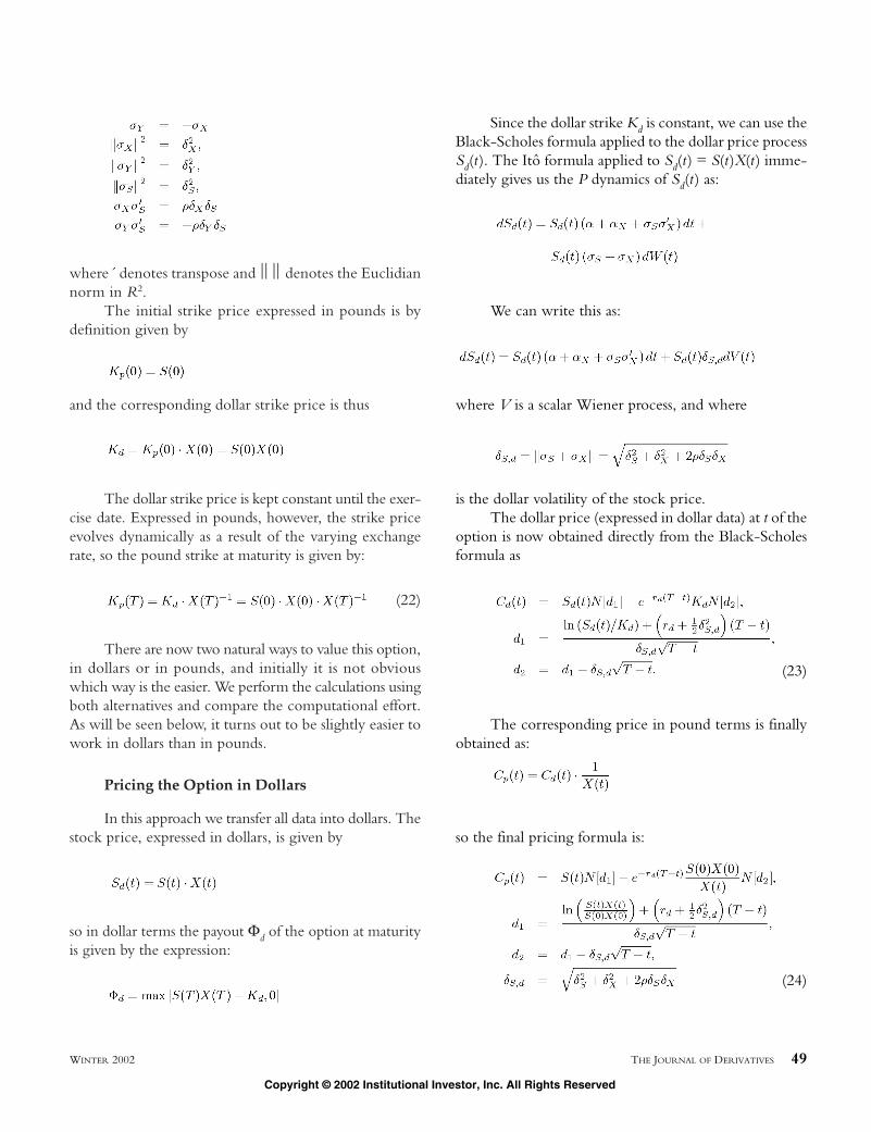
where ´ denotes transpose and denotes the Euclidiannorm in R2.

The initial strike price expressed in pounds is bydefinition given by

and the corresponding dollar strike price is thus

The dollar strike price is kept constant until the exer-cise date. Expressed in pounds, however, the strike priceevolves dynamically as a result of the varying exchangerate, so the pound strike at maturity is given by:

(22)

There are now two natural ways to value this option,in dollars or in pounds, and initially it is not obviouswhich way is the easier. We perform the calculations usingboth alternatives and compare the computational effort.As will be seen below, it turns out to be slightly easier towork in dollars than in pounds.

Pricing the Option in Dollars

In this approach we transfer all data into dollars. Thestock price, expressed in dollars, is given by

so in dollar terms the payout Φd of the option at maturityis given by the expression:

Since the dollar strike Kd is constant, we can use theBlack-Scholes formula applied to the dollar price processSd(t). The Itô formula applied to Sd(t) = S(t)X(t) imme-diately gives us the P dynamics of Sd(t) as:

We can write this as:

where V is a scalar Wiener process, and where

is the dollar volatility of the stock price.The dollar price (expressed in dollar data) at t of the

option is now obtained directly from the Black-Scholesformula as

(23)

The corresponding price in pound terms is finallyobtained as:

so the final pricing formula is:

(24)



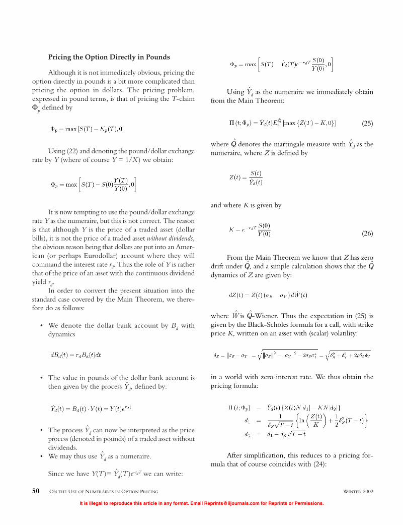
Pricing the Option Directly in Pounds

Although it is not immediately obvious, pricing theoption directly in pounds is a bit more complicated thanpricing the option in dollars. The pricing problem,expressed in pound terms, is that of pricing the T-claimΦp defined by

Using (22) and denoting the pound/dollar exchangerate by Y (where of course Y = 1/X ) we obtain:

It is now tempting to use the pound/dollar exchangerate Y as the numeraire, but this is not correct. The reasonis that although Y is the price of a traded asset (dollarbills), it is not the price of a traded asset without dividends,the obvious reason being that dollars are put into an Amer-ican (or perhaps Eurodollar) account where they willcommand the interest rate rd. Thus the role of Y is ratherthat of the price of an asset with the continuous dividendyield rd.

In order to convert the present situation into thestandard case covered by the Main Theorem, we there-fore do as follows:

• We denote the dollar bank account by Bd withdynamics

• The value in pounds of the dollar bank account isthen given by the process Yd, defined by:

• The process Yd can now be interpreted as the priceprocess (denoted in pounds) of a traded asset withoutdividends.

• We may thus use Yd as a numeraire.

Since we have Y(T )= Yd(T )e–rdT we can write:

Using Yd as the numeraire we immediately obtainfrom the Main Theorem:

(25)

where Q denotes the martingale measure with Yd as thenumeraire, where Z is defined by

and where K is given by

(26)

From the Main Theorem we know that Z has zerodrift under Q, and a simple calculation shows that the Qdynamics of Z are given by:

where W is Q-Wiener. Thus the expectation in (25) isgiven by the Black-Scholes formula for a call, with strikeprice K, written on an asset with (scalar) volatility:

in a world with zero interest rate. We thus obtain thepricing formula:

After simplification, this reduces to a pricing for-mula that of course coincides with (24):



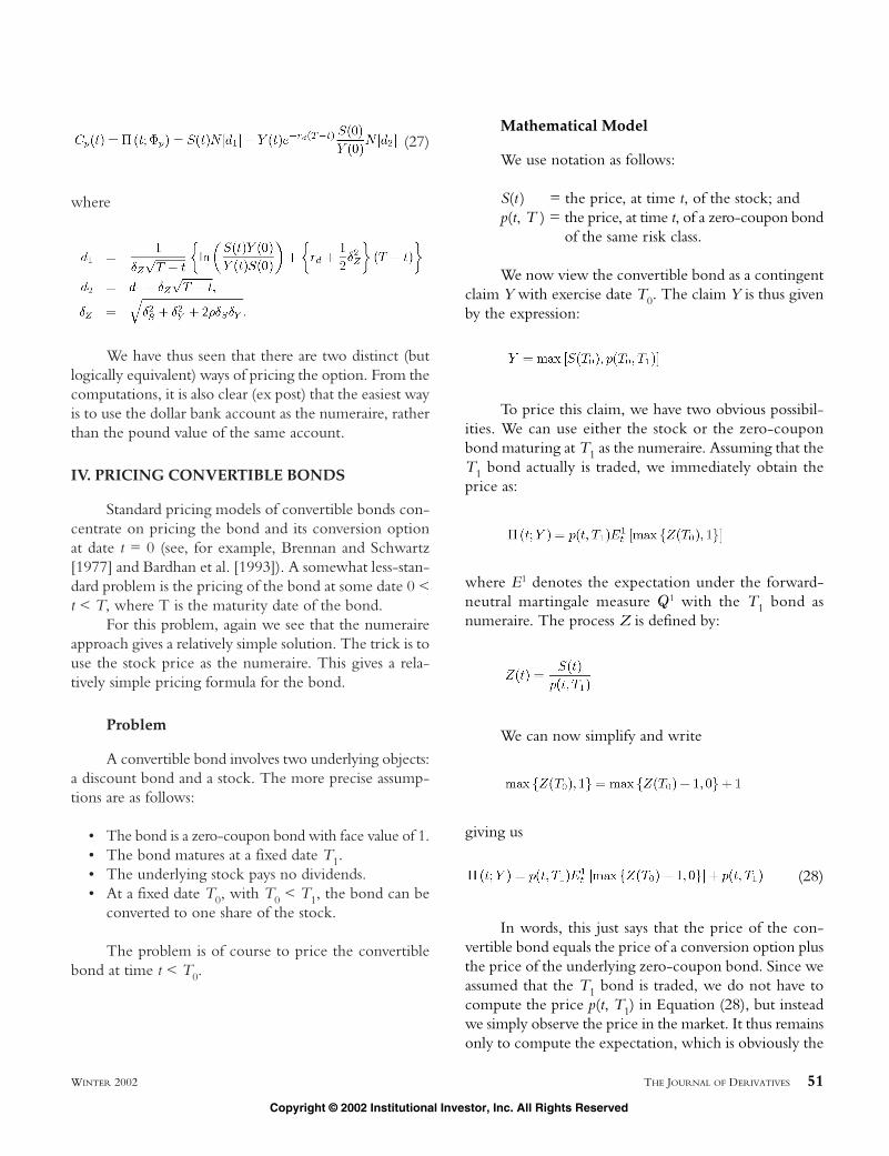
(27)

where

We have thus seen that there are two distinct (butlogically equivalent) ways of pricing the option. From thecomputations, it is also clear (ex post) that the easiest wayis to use the dollar bank account as the numeraire, ratherthan the pound value of the same account.

IV. PRICING CONVERTIBLE BONDS

Standard pricing models of convertible bonds con-centrate on pricing the bond and its conversion optionat date t = 0 (see, for example, Brennan and Schwartz[1977] and Bardhan et al. [1993]). A somewhat less-stan-dard problem is the pricing of the bond at some date 0 <t < T, where T is the maturity date of the bond.

For this problem, again we see that the numeraireapproach gives a relatively simple solution. The trick is touse the stock price as the numeraire. This gives a rela-tively simple pricing formula for the bond.

Problem

A convertible bond involves two underlying objects:a discount bond and a stock. The more precise assump-tions are as follows:

• The bond is a zero-coupon bond with face value of 1.• The bond matures at a fixed date T1.• The underlying stock pays no dividends.• At a fixed date T0, with T0 < T1, the bond can be

converted to one share of the stock.

The problem is of course to price the convertiblebond at time t < T0.

Mathematical Model

We use notation as follows:

S(t ) = the price, at time t, of the stock; andp(t, T ) = the price, at time t, of a zero-coupon bond

of the same risk class.

We now view the convertible bond as a contingentclaim Y with exercise date T0. The claim Y is thus givenby the expression:

To price this claim, we have two obvious possibil-ities. We can use either the stock or the zero-couponbond maturing at T1 as the numeraire. Assuming that theT1 bond actually is traded, we immediately obtain theprice as:

where E1 denotes the expectation under the forward-neutral martingale measure Q1 with the T1 bond asnumeraire. The process Z is defined by:

We can now simplify and write

giving us

(28)

In words, this just says that the price of the con-vertible bond equals the price of a conversion option plusthe price of the underlying zero-coupon bond. Since weassumed that the T1 bond is traded, we do not have tocompute the price p(t, T1) in Equation (28), but insteadwe simply observe the price in the market. It thus remainsonly to compute the expectation, which is obviously the



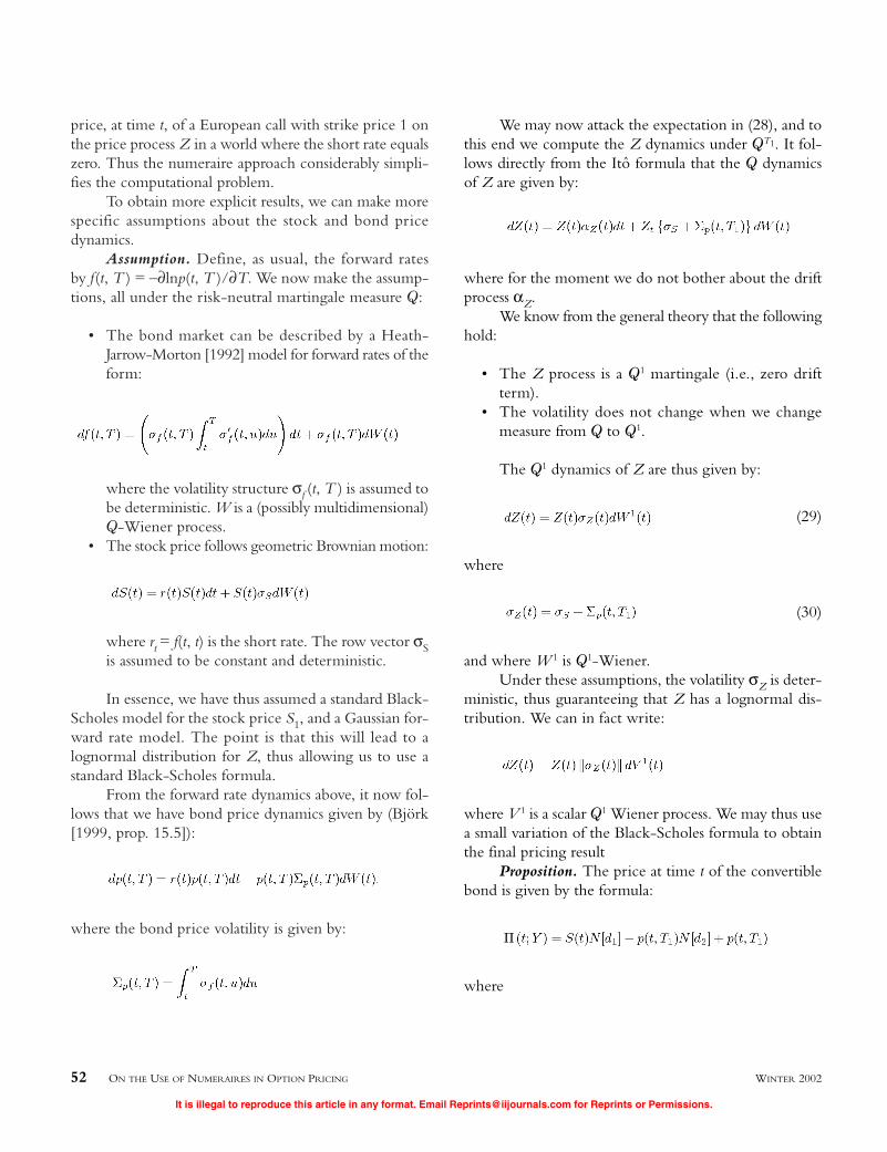
price, at time t, of a European call with strike price 1 onthe price process Z in a world where the short rate equalszero. Thus the numeraire approach considerably simpli-fies the computational problem.

To obtain more explicit results, we can make morespecific assumptions about the stock and bond pricedynamics.

Assumption. Define, as usual, the forward rates by f(t, T ) = –∂lnp(t, T )/∂T. We now make the assump-tions, all under the risk-neutral martingale measure Q:

• The bond market can be described by a Heath-Jarrow-Morton [1992] model for forward rates of theform:

where the volatility structure σf (t, T ) is assumed tobe deterministic. W is a (possibly multidimensional)Q-Wiener process.

• The stock price follows geometric Brownian motion:

where rt = f(t, t) is the short rate. The row vector σSis assumed to be constant and deterministic.

In essence, we have thus assumed a standard Black-Scholes model for the stock price S1, and a Gaussian for-ward rate model. The point is that this will lead to alognormal distribution for Z, thus allowing us to use astandard Black-Scholes formula.

From the forward rate dynamics above, it now fol-lows that we have bond price dynamics given by (Björk[1999, prop. 15.5]):

where the bond price volatility is given by:

We may now attack the expectation in (28), and tothis end we compute the Z dynamics under QT1. It fol-lows directly from the Itô formula that the Q dynamicsof Z are given by:

where for the moment we do not bother about the driftprocess αZ.

We know from the general theory that the followinghold:

• The Z process is a Q1 martingale (i.e., zero driftterm).

• The volatility does not change when we changemeasure from Q to Q1.

The Q1 dynamics of Z are thus given by:

(29)

where

(30)

and where W 1 is Q1-Wiener. Under these assumptions, the volatility σZ is deter-

ministic, thus guaranteeing that Z has a lognormal dis-tribution. We can in fact write:

where V 1 is a scalar Q1 Wiener process. We may thus usea small variation of the Black-Scholes formula to obtainthe final pricing result

Proposition. The price at time t of the convertiblebond is given by the formula:

where



V. PRICING SAVINGS PLANS WITH CHOICEOF INDEXING

Savings plans that offer the saver some choice aboutthe measure affecting rates are common. Typically theygive savers an ex post choice of the interest rate to be paidon their account. With the inception of capital require-ments, many financial institutions have to recognize theseoptions and price them.

Problem

We use as an example a bank account in Israel. Thisaccount gives savers the ex post choice of indexing theirsavings to an Israeli shekel interest rate or a U.S. dollarrate.

• The saver deposits NIS 100 (Israeli shekels) today ina shekel/dollar savings account with a maturity ofone year.

• In one year, the account pays the maximum of:

° The sum of NIS 100 + real shekel interest, the wholeamount indexed to the inflation rate; or

° Today’s dollar equivalent of NIS 100 + dollarinterest, the whole amount indexed to the dollarexchange rate.

The savings plan is thus an option to exchange theIsraeli interest rate for the U.S. interest rate, while at thesame time taking on exchange rate risk. Since the choiceis made ex post, it is clear that both the shekel and thedollar interest rates offered on such an account must bebelow the respective market rates.

Mathematical Model

We consider two economies, one domestic and oneforeign, using notation as follows:

rd = domestic short rate;rf = foreign short rate;I(t) = domestic inflation process;X(t) = the exchange rate in terms of domestic

currency/foreign currency;Y(t) = the exchange rate in terms of foreign

currency/domestic currency; andT = the maturity date of the savings plan.

The value of the option is linear in the initial shekelamount invested in the savings plan; without loss of gen-erality, we assume that this amount is one shekel. In thedomestic currency, the contingent T-claim Φd to be pricedis thus given by:

In the foreign currency, the claim Φf is given by:

It turns out that it is easier to work with Φf thanwith Φd, and we have

The price (in the foreign currency) at t = 0 of thisclaim is now given by

(31)

where Qf denotes the risk-neutral martingale measure forthe foreign market.

At this point, we have to make some probabilisticassumptions. We assume that we have a Garman-Kohlhagen [1983] model for Y. Standard theory thengives us the Qf dynamics of Y as



(32)

For simplicity we assume also that the price levelfollows a geometric Brownian motion, with Qf dynamicsgiven by

(33)

Note that W is assumed to be two-dimensional, thusallowing for correlation between Y and I. Also note thateconomic theory does not say anything about the meaninflation rate αI under Qf .

When we compute the expectation in Equation(31), we cannot use a standard change of numeraire tech-nique, because none of the processes Y, I, or YI are priceprocesses of traded assets without dividends. Instead wehave to attack the expectation directly.

To that end we define the process Z as Z(t) = Y(t)I(t), and obtain the Qf dynamics:

From this it is easy to see that if we define S(t) by

then we will have the Qf dynamics

Thus, we can interpret S(t) as a stock price in aBlack-Scholes world with zero short rate and Qf as therisk-neutral measure. With this notation we easily obtain:

where

The expectation can now be expressed by the Black-Scholes formula for a call option with strike price e–cTY(0),zero short rate, and volatility given by:

The price at t = 0 of the claim expressed in the for-eign currency is thus given by the formula:

(34)

Finally, the price at t = 0 in domestic terms is givenby

(35)

For practical purposes it may be more convenientto model Y and I as

where now σY and σY are constant scalars, while WY andWI are scalar Wiener processes with local correlation givenby dWY(t)dWI(t) = ρdt.

In this model (which of course is logically equiva-lent to the one above), we have the pricing formulas (34)-(35), but now with the notation

VI. ENDOWMENT WARRANTS

Endowment options, which are primarily traded inAustralia and New Zealand, are very long-term calloptions on equity. These options are discussed by Hoang,Powell, and Shi [1999] (henceforth HPS).

∏ ∏=

−

( ; ) ( ; )

( ) [ ] [ ]

0 0

1 2

X

= e +cT

Φ Φd f

I N d N d

(0)

0 1



Endowment warrants have two unusual features. Theirdividend protection consists of adjustments to the strikeprice, and the strike price behaves like a money market fund(i.e., increases over time at the short-term interest rate). HPSassume that the dividend adjustment to the strike price isequivalent to the usual dividend adjustment to the stockprice; this assumption is now known to be mistaken.3 Underthis assumption they obtain an arbitrage-free warrant pricewhere the short rate is deterministic, and provide an approx-imation of the option price under stochastic interest rate.

We discuss a pseudo-endowment option. This pseudo-endowment option is like the Australian option, exceptthat its dividend protection is the usual adjustment to thestock price (i.e., the stock price is raised by the dividends).The pseudo-endowment option thus depends on twosources of uncertainty: the (dividend-adjusted) stock priceand the short-term interest rate.

With a numeraire approach, we can eliminate one ofthese sources of risk. Choosing an interest rate-related instru-ment (i.e., a money market account) as a numeraire resultsin a pricing formula for the pseudo-endowment optionthat is similar to the standard Black-Scholes formula.4

Problem

A pseudo-endowment option is a very long-termcall option. Typically the characteristics are as follows:

• At issue, the initial strike price K(0) is set to approx-imately 50% of the current stock price, so the optionis initially deep in the money.

• The endowment options are European.• The time to exercise is typically ten-plus years.• The options are interest rate and dividend protected.

The protection is achieved by two adjustments:

° The strike price is not fixed over time. Instead itgrows at the short-term interest rate.

° The stock price is increased by the amount of thedividend each time a dividend is paid.

• The payoff at the exercise date T is that of a stan-dard call option, but with the adjusted (as above)strike price K(T ).

Mathematical Model

We model the underlying stock price process S(t) ina standard Black-Scholes setting. In other words, under theobjective probability measure P, the price process S(t) fol-lows geometric Brownian motion (between dividends) as:

where α and σ are deterministic constants, and Wp is a PWiener process. We allow the short rate r to be an arbi-trary random process, thus giving the P dynamics of themoney market account as:

(36)

(37)

To analyze this option, we have to formalize theprotection features of the option as follows.

• We assume that the strike price process K(t) is changedat the continuously compounded instantaneousinterest rate. The formal model is thus as follows:

(38)

• For simplicity, we assume that the dividend protec-tion is perfect. More precisely, we assume that thedividend protection is obtained by reinvesting thedividends in the stock itself. Under this assumption,we can view the stock price as the theoretical priceof a mutual fund that includes all dividends investedin the stock. Formally this implies that we can treatthe stock price process S(t) as the price process of astock without dividends.

The value of the option at the exercise date T isgiven by the contingent claim Y, defined by

Clearly there are two sources of risk in endowmentoptions: stock price risk, and the risk of the short-terminterest rate. In order to analyze this option, we observethat from (36)-(38) it follows that:

Thus we can express the claim Y as:



From this expression, we see that the natural numeraireprocess is now obviously the money account B(t). Themartingale measure for this numeraire is the standard risk-neutral martingale measure Q under which we have thestock price dynamics:

(39)

where W is a Q-Wiener process.A direct application of the Main Theorem gives us

the pricing formula:

After a simple algebraic manipulation, and using thefact that B(0) = 1, we thus obtain

(40)

where Z(t) = S(t)/B(t) is the normalized stock price pro-cess. It follows immediately from (36), (39), and the Itôformula that under Q we have Z dynamics given by

(41)

and from (40)-(41), we now see that our original pricingproblem has been reduced to computing the price of astandard European call, with strike price K(0), on anunderlying stock with volatility σ in a world where theshort rate is zero.

Thus the Black-Scholes formula gives the endow-ment warrant price at t = 0 directly as:

(42)

where

Using the numeraire approach, the price of theendowment option in (42) is given by a standard Black-Scholes formula for the case where r = 0. The result does

not in any way depend upon assumptions made about thestochastic short rate process r(t).

The pricing formula (42) is in fact derived in HPS[1999] but only for the case of a deterministic short rate.The case of a stochastic short rate is not treated in detail.Instead HPS attempt to include the effect of a stochasticinterest rate as follows:

• They assume that the short rate r is deterministicand constant.

• The strike price process is assumed to have dynamicsof the form

where V is a new Wiener process (possibly corre-lated with W ).

• They value the claim Y =max[S(T ) – K(T ), 0] byusing the Margrabe [1978] result about exchangeoptions.

HPS claim that this setup is an approximation of thecase of a stochastic interest rate. Whether it is a goodapproximation or not is never clarified, and from our anal-ysis above we can see that the entire scheme is in factunnecessary, since the pricing formula in Equation (42)is invariant under the introduction of a stochastic short rate.

Note that our result relies upon our simplifyingassumption about perfect dividend protection. A morerealistic modeling of the dividend protection would leadto severe computation problems. To see this, assume thatthe stock pays a constant dividend yield rate δ. This wouldchange our model in two ways. The Q dynamics of thestock price would be different, and the dynamics of thestrike process K(t) would have to be changed.

As for the Q dynamics of the stock price, standardtheory immediately gives us:

Furthermore, from the problem description, we seethat in real life (rather than in a simplified model), dividendprotection is obtained by reducing the strike price processby the dividend amount at every dividend payment. In termsof our model, this means that over an infinitesimal interval[t, t + dt], the strike price should drop by the amount δS(t)dt.



Thus the K dynamics are given by

This equation can be solved as:

The moral is that in the expression of the contin-gent claim

we now have the awkward integral expression

Even in the simple case of a deterministic short rate,this integral is quite problematic. It is then basically a sum oflognormally distributed random variables, and thus we havethe same difficult computation problems for Asian options.

VII. CONCLUSION

Numeraire methods have been in the derivativespricing literature since Geman [1989] and Jamshidian[1989]. These methods afford a considerable simplifica-tion in the pricing of many complex options, but theyappear not to be well known.

We have considered five problems whose computa-tion is vastly aided by the use of numeraire methods. Wediscuss the pricing of employee stock ownership plans;the pricing of options whose strike price is denominatedin a currency different from that of the underlying stock;the pricing of convertible bonds; the pricing of savingsplans where the choice of interest paid is ex post chosenby the saver; and finally, the pricing of endowment options.

Numeraire methods are not a cure-all for complexoption pricing, although when there are several risk factorsthat impact an option’s price, choosing one of the factorsas a numeraire reduces the dimensionality of the compu-tation problem by one. Smart choice of the numeraire can,in addition, produce significant computational simplifica-tion in an option’s pricing.

ENDNOTES

Benninga thanks the Israel Institute of Business Researchat Tel-Aviv University for a grant. Wiener’s research was fundedby the Krueger Center at the Hebrew University of Jerusalem.

1Readers interested only in implementation of thenumeraire method can skip over this section.

2For tax reasons, most executive stock options are initiallyat the money.

3Brown and Davis [2001].4This formula was derived by HPS as a solution for the

deterministic interest rate.

REFERENCES

Bardhan I., A. Bergier, E. Derman, C. Dosemblet, I. Kani, andP. Karasinski. “Valuing Convertible Bonds as Derivatives.”Goldman Sachs Quantitative Strategies Research Notes, 1993.

Björk, T. Arbitrage Theory in Continuous Time. Oxford: OxfordUniversity Press, 1999.

Brennan, M.J., and E.S. Schwartz. “Convertible Bonds: Val-uation and Optimal Strategies for Call and Conversion.” Journalof Finance, 32 (1977), pp. 1699-1715.

Brenner, M., and D. Galai. “The Determinants of the Returnon Index Bonds.” Journal of Banking and Finance, 2 (1978), pp.47-64.

Brown, C., and K. Davis. “Dividend Protection at a Price:Lessons from Endowment Warrants.” Working paper, Uni-versity of Melbourne, 2001.

Fischer, S. “Call Option Pricing When the Exercise Price IsUncertain, and the Valuation of Index Bonds.” Journal of Finance,33 (1978), pp. 169-176.

Garman, M.B., and S.W. Kohlhagen. “Foreign CurrencyOption Values.” Journal of International Money and Finance, 2(1983), pp. 231-237.

Geman, H. “The Importance of Forward Neutral Probabilityin a Stochastic Approach of Interest Rates.” Working paper,ESSEC, 1989.

Geman, H., N. El Karoui, and J.C. Rochet. “Change ofNumeraire, Changes of Probability Measures and Pricing ofOptions.” Journal of Applied Probability, 32 (1995), pp. 443-458.

Harrison, J., and J. Kreps. “Martingales and Arbitrage in Mul-tiperiod Securities Markets.” Journal of Economic Theory, 11(1981), pp. 418-443.



Harrison, J., and S. Pliska. “Martingales and Stochastic Integralsin the Theory of Continuous Trading.” Stochastic Processes Appli-cations, 11 (1981), pp. 215-260.

Harrison, J.M., and D. Kreps. “Martingales and Arbitrage inMultiperiod Securities Markets.” Journal of Economic Theory, 20(1979), pp. 381-408.

Haug, E.G. The Complete Guide to Option Pricing Formulas. NewYork: McGraw-Hill, 1997.

Heath, D., R. Jarrow, and A. Morton. “Bond Pricing and theTerm Structure of Interest Rates: A New Methodology.” Econo-metrica, 60 (1992), pp. 77-105.

Hoang, Philip, John G. Powell, and Jing Shi. “Endowment Wa-rrant Valuation.” The Journal of Derivatives, 7 (1999), pp. 91-103.

Jamshidian, F. “An Exact Bond Option Formula.” Journal ofFinance, 44 (1989), pp. 205-209.

Margrabe, W. “The Value of an Option to Exchange One Assetfor Another.” Journal of Finance, 33, 1 (1978), pp. 177-186.

Merton, Robert C. “A Rational Theory of Option Pricing.”Bell Journal of Economics and Management Science, 4 (1973), pp.141-183.

To order reprints of this article, please contact Ajani Malik [email protected] or 212-224-3205.



Documents

On the Use of Numeraires in Option Pricing IT IS ILLEGAL ...rolf/teaching/PhDcourse/BBWnumeraire.pdf · On the Use of Numeraires in Option Pricing SIMON BENNINGA, TOMAS BJÖRK, AND