Embed Size (px)
Citation preview

2013
UNIVERSITY OF PISA
Engineering PhD School “Leonardo da Vinci”
PhD Course in
“Applied Electromagnetism in Electrical and Biomedical Engineering,
Electronics, Smart Sensors, Nano-Technologies”
XXV Course
PhD Thesis
On the use of electromagnetic
asymptotic methods for the estimation
of communications propagation
channel in complex environments.
ING/INF-02
Advisors:
Prof. Agostino MONORCHIO
_____________________________
Prof. Paolo NEPA
_____________________________
Author:
Pierpaolo USAI
_____________________________

Copyright © Pierpaolo Usai, 2013

To my parents


Pierpaolo Usai
Contents
1
Contents
Contents ........................................................................................................................... 1
Publications ...................................................................................................................... 4
Introduction ...................................................................................................................... 7
1 The Ray Tracing Method............................................................................................ 9
1.1 Multipath and electromagnetic solver .............................................................. 10
1.2 RT Algorithm ................................................................................................... 11
1.3 Direct contribution ........................................................................................... 12
1.4 Reflection contribution .................................................................................... 14
1.5 Diffraction contribution ................................................................................... 15
1.6 Transmission contribution ................................................................................ 18
2 Arbitrary Voxel Selection......................................................................................... 21
2.1 Algorithm description ...................................................................................... 23
2.2 The algorithm validation for a test-case urban scenario ................................... 25
2.3 The algorithm performance evaluation ............................................................ 28
3 Channel Characterization by a Ray Tracing Analysis .............................................. 33
3.1 Frequency response .......................................................................................... 34
3.1.1 Narrow band signal ............................................................................... 35
3.1.2 Wide band signal .................................................................................. 36
3.2 Channel definitions .......................................................................................... 36
3.2.1 Antenna transfer function ..................................................................... 37
3.3 Impulse response .............................................................................................. 38
3.3.1 Base band system .................................................................................. 39

Pierpaolo Usai
Contents
2
3.3.2 Pass band system ................................................................................... 39
3.3.3 Power Delay Profile and Delay Spread evaluation ................................ 40
3.4 Spreading function ............................................................................................ 40
3.5 Baseband Test Case .......................................................................................... 41
3.6 Passband Test Case ........................................................................................... 44
4 Estimation of Airport Surface Propagation Channel ................................................. 49
4.1 Measurement campaign in Munich airport ....................................................... 51
4.2 3D model of a typical airport environment ....................................................... 52
4.2.1 The Munich airport model validation: received power ......................... 54
4.3 Spreading function ............................................................................................ 55
4.3.1 The direct deterministic approach ......................................................... 55
4.4 Munich Airport Results .................................................................................... 57
4.4.1 Measured and estimated spreading function ......................................... 57
4.4.2 The scatter position evaluation .............................................................. 58
4.4.3 Spreading function trend along the R1-R2-R3 path .............................. 60
4.5 Simulation time comparison ............................................................................. 63
5 Scattering Matrix....................................................................................................... 67
5.1 Scattering Matrix .............................................................................................. 69
5.2 PO based numerical solver ............................................................................... 70
5.3 PO surface currents ........................................................................................... 71
5.3.1 Free space propagation .......................................................................... 72
5.3.2 The studied propagation problem. ......................................................... 72
5.3.3 Formulation for a PEC object ................................................................ 73
5.3.4 Formulation for a dielectric object ........................................................ 75
5.4 PO radiation integral ......................................................................................... 75
5.4.1 PEC object ............................................................................................. 75
5.4.2 Dielectric object .................................................................................... 76
5.4.3 Solution of the radiation integral on a triangular domain ...................... 76
5.5 Estimation of the RCS parameter ..................................................................... 77
5.5.1 Case of study: PEC dodecahedron ........................................................ 77
5.5.2 Case of study: dielectric dodecahedron ................................................. 79

Pierpaolo Usai
Contents
3
5.5.3 Simulation time comparison ................................................................. 79
5.6 RCS Spectrum of rotating objects .................................................................... 81
5.6.1 Case of study: 2-blades ......................................................................... 81
Appendix A – Radiation Integral on a triangular space domain .................................... 83
Conclusions .................................................................................................................... 87
Bibliography .................................................................................................................. 89
Acknowledgments .......................................................................................................... 93

Pierpaolo Usai
Publications
4
Publications
Conference and Journal
E.1 P. Usai, A. Corucci, S. Genovesi, A. Monorchio, “Arbitrary Voxel Selection
For Accelerating A Ray Tracing-Based Field Prediction Model In Urban
Environments”, Electromagnetic Waves and Progress in Electromagnetic
Research C, No. 20, pp. 43-53, 2011.
E.2 P. Usai, A. Corucci, S. Genovesi, A. Monorchio, "Arbitrary Voxel Selection
for Speeding up a Ray Tracing-based EM Simulator", IEEE Antennas and
Propagation Symposium, 2010, Toronto-Canada.
E.3 P. Usai, A. Corucci, A. Monorchio, S. Gligorevich, “Estimation of Airport
Surface Propagation Channel: Ray Tracing Model and Measurements”,
European Conference of Antennas and Propagation, EUCAP2011, Rome,
Italy, April 11-15, 2011.
E.4 P. Usai, A. Monorchio, A. Pellegrini, A. Brizzi, Lianhong Zhang, Yang Hao,
“Analysis of On-Body Propagation at W Band by Using Ray Tracing Model
and Measurements”, IEEE International Symposium on Antennas and
Propagation and USNC-URSI National Radio Science Meeting, APS-URSI
2012,Chicago,USA, July 2012.
E.5 G. Nastasia, P. Usai, A. Corucci, A. Monorchio, “Wireless Channel
Characterization On Board a Ship by Using an Efficient Ray-Tracing
Simulator”, IEEE International Symposium on Antennas and Propagation and
USNC-URSI National Radio Science Meeting, APS-URSI 2012,Chicago,USA,
July 2012.
Pierpaolo Usai
Publications
5
Technical report
E.1 A. Corucci, P. Usai, A. Monorchio, “Previsioni dell’esposizione ai campi
elettromagnetici nei dintorni della postazione PISQ sita nel comune di
Tortolì", NAMSA Project, Convenzione DII-Ambiente s.c., Pisa, Apr. 2010.
E.2 S. Gligorevic, P. Usai, A. Ruggeri, “D6.2.2-Report on Modeling and
Performance Simulations”, SANDRA Project, Wessling, Munich, Germany,
Oct. 2011.
E.3 P. Usai, A. Corucci, S. Genovesi, D. Bianchi, A. Rogovich, A. Monorchio,
"Misura e caratterizzazione dei prototipi in termini di diagramma di
irradiazione, guadagno e impedenza di ingresso in spazio libero", SHIRED
Project, CNIT, Pisa, Jun. 2012.
E.4 P. Usai, M. De Gregorio, A. Rogovich, A. Monorchio, "Metodi di misura e
caratterizzazione dei prototipi montati su modelli in scala di unità navali",
SHIRED Project, CNIT, Pisa, Jul. 2012.
E.5 P. Usai, M. De Gregorio, N. Fontana, A. Monorchio, "Relazione sulle attività
sperimentali condotte nella fase 2", SHIRED Project, CNIT, Pisa, Sept. 2012.

Pierpaolo Usai
Publications
6
Pierpaolo Usai
Introduction
7
Introduction
Before planning and realizing wireless communication systems, exact propagation
characteristics of the environment should be known. Many empirical, statistical and
physical models are used for this purpose. Among the asymptotic methods, inverse 3D
deterministic ray tracing models are characterized by an accurate prediction of the
electromagnetic field both in the case of an outdoor site as well as an indoor location. In
radio frequency system planning, the ray tracing propagation model and data of the
scenario can be used to predict the radio frequency coverage area of a transmitter. This
analysis allows to determine the received signal strength at the receiver, the path-loss of
a wireless link and channel impairment such as delay spread due to multi-path fading.
The knowledge of these parameters before the wireless system setting-up leads to an
installation cost reduction together with a quality of services increase. For example, it is
possible to estimate the minimum number of antennas and their best locations in order
to guarantee a suitable radio frequency coverage of an area. Then, the 'in situ'
measurements can be carried out as an 'a posteriori' check for validate the predicted
results. Moreover, the level of the electromagnetic radiation can be accurately predicted
in order to investigate possible health hazards or to test the fulfillment of the limits of
exposition defined in norms and recommendations.
The ray tracing method and the high frequency theories this method is based on are
recapitulated in chapter 1 in the formulation implemented in the software EMviroment-
EMv used in this thesis to predict the electromagnetic propagation in complex
environment. The estimation of channel parameters by asymptotic propagation model
based software could show some drawbacks, such as long simulation times caused by
the multipath reconstruction, and a huge memory dimension requirement to store the
multipath info that is useful for the frequency analysis of the channel. A lot of energies
were spent in optimizing and speeding up the ray tracing algorithms by researchers in
the last decades. In the implementation of ray tracing based solver the study of the
acceleration of the geometrical algorithm to predict the multipath has a great
importance, because the physical coherence of this deterministic approach leads to a
boost of the computational time. A method for speeding up a ray tracing based electric
field prediction model suitable for urban environments investigation is described in
chapter 2.

Pierpaolo Usai
Introduction
8
The physical coherence of this high frequency method allows to accurately estimate
the wireless communication channel frequency response and the antennas influence on
the transmitted and received signals. A frequency analysis of the channel is required, for
example, in ultra-wideband applications. In this case the frequency selective behavior of
the channel needs to be estimate to correctly predict the communication link
impairment. The frequency response definition by multipath prediction is shown in
chapter 3
The Doppler frequency shift is caused by the presence of relative movement by the
transmitter, the receiver and the complex objects present in the scene. The power
distribution in the Doppler frequency shift domain can be derived by the spreading
function estimation. By definition the spreading function could be calculated starting
from the knowledge of the impulse response of a channel link by means of the Fourier
transform. An alternative direct deterministic approach for its estimation avoiding the
Fourier transform has been formulated and is presented in chapter 4 applied to the
Munich airport complex scenario.
The radar cross section evaluation of metal and dielectric objects needs to invoke the
asymptotic techniques to overcome the limitations the full-wave techniques present at
high frequencies. The method of moments, for example, needs a denser and denser
mesh definition of the studied object as the wavelength decreases to respect the
applicability constraints of the method. Because the complexity of this method is
proportional to the currents on the facets, the number of unknowns can get to saturate
the computer memory availability and increase the simulation time. The approximations
that can be introduced with the assumption of far-field sources and observers at high
frequencies allow to unburden the calculation procedures obtaining good estimations of
the scattered field. The Physical Optics - PO theory is the most diffuse solution solving
these kind of problems, often together with a ray bouncing analysis to predict the
illuminated facets of the object. A PO based solver to predict the scattered field by a
metallic or dielectric object and the radar cross section spectrum of rotating objects is
presented in chapter 5.
Pierpaolo Usai 1The Ray Tracing Method
9
1 The Ray Tracing Method
Ray propagation, multipath prediction and types of
contribution in a ray tracing based propagation
model.
According to the asymptotic high frequency techniques arising from the Geometrical
Optics (GO), Geometrical Theory of Diffraction (GTD) and its extension Uniform
Theory of Diffraction (UTD), when the dimensions of the obstacles constituting the
scenario are much larger than the wavelength λ of the signal (typically 10λ), it is
possible to use the concept of ray to study the radio propagation and to predict the effect
that the electromagnetic wave undergoes interacting with the environment during its
path. An electromagnetic wave radiated by the source (transmitting antenna Tx) in a
scenario, reaches the point of observation (receiving antenna Rx) after various bounces
induced by different physical phenomena. The GO [1] provides for the propagation
along the line between Tx and Rx (direct ray) and the propagation by reflection and
transmission on the surfaces of obstacles that compose the scenario (reflected rays and
transmitted rays). The GTD [2] provides for the propagation by diffraction from the
edges in common between two surfaces (diffracted rays). These rays allow the
electromagnetic wave to reach the shadowed areas of a scenario.
Pierpaolo Usai
1 The Ray Tracing Method
10
1.1 Multipath and electromagnetic solver
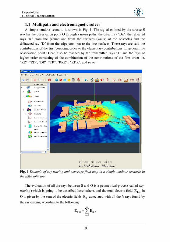
A simple outdoor scenario is shown in Fig. 1. The signal emitted by the source S
reaches the observation point O through various paths: the direct ray "Dir", the reflected
rays "R" from the ground and from the surfaces (walls) of the obstacles and the
diffracted ray "D" from the edge common to the two surfaces. These rays are said the
contributions of the first bouncing order or the elementary contributions. In general, the
observation point O can also be reached by the transmitted rays "T" and the rays of
higher order consisting of the combination of the contributions of the first order i.e.
"RR", "RD", "DR", "TR", "RRR" , "RDR", and so on.
Fig. 1 Example of ray tracing and coverage field map in a simple outdoor scenario in
the EMv software.
The evaluation of all the rays between S and O is a geometrical process called ray-
tracing (which is going to be described hereinafter), and the total electric field TotE in
O is given by the sum of the electric fields nE associated with all the N rays found by
the ray-tracing according to the following
1=
=∑Tot nE E
N
n
.
Pierpaolo Usai 1The Ray Tracing Method
11
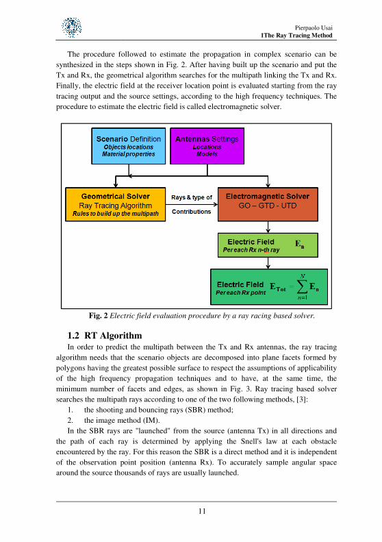
The procedure followed to estimate the propagation in complex scenario can be
synthesized in the steps shown in Fig. 2. After having built up the scenario and put the
Tx and Rx, the geometrical algorithm searches for the multipath linking the Tx and Rx.
Finally, the electric field at the receiver location point is evaluated starting from the ray
tracing output and the source settings, according to the high frequency techniques. The
procedure to estimate the electric field is called electromagnetic solver.
Fig. 2 Electric field evaluation procedure by a ray racing based solver.
1.2 RT Algorithm
In order to predict the multipath between the Tx and Rx antennas, the ray tracing
algorithm needs that the scenario objects are decomposed into plane facets formed by
polygons having the greatest possible surface to respect the assumptions of applicability
of the high frequency propagation techniques and to have, at the same time, the
minimum number of facets and edges, as shown in Fig. 3. Ray tracing based solver
searches the multipath rays according to one of the two following methods, [3]:
1. the shooting and bouncing rays (SBR) method;
2. the image method (IM).
In the SBR rays are "launched" from the source (antenna Tx) in all directions and
the path of each ray is determined by applying the Snell's law at each obstacle
encountered by the ray. For this reason the SBR is a direct method and it is independent
of the observation point position (antenna Rx). To accurately sample angular space
around the source thousands of rays are usually launched.
Pierpaolo Usai
1 The Ray Tracing Method
12
Fig. 3 Decomposition of a building into polygons
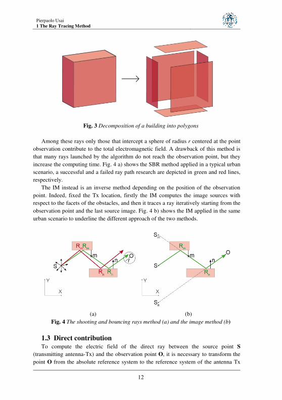
Among these rays only those that intercept a sphere of radius r centered at the point
observation contribute to the total electromagnetic field. A drawback of this method is
that many rays launched by the algorithm do not reach the observation point, but they
increase the computing time. Fig. 4 a) shows the SBR method applied in a typical urban
scenario, a successful and a failed ray path research are depicted in green and red lines,
respectively.
The IM instead is an inverse method depending on the position of the observation
point. Indeed, fixed the Tx location, firstly the IM computes the image sources with
respect to the facets of the obstacles, and then it traces a ray iteratively starting from the
observation point and the last source image. Fig. 4 b) shows the IM applied in the same
urban scenario to underline the different approach of the two methods.
(a) (b)
Fig. 4 The shooting and bouncing rays method (a) and the image method (b)
1.3 Direct contribution
To compute the electric field of the direct ray between the source point S
(transmitting antenna-Tx) and the observation point O, it is necessary to transform the
point O from the absolute reference system to the reference system of the antenna Tx

Pierpaolo Usai 1The Ray Tracing Method
13
(point Os) that can be arbitrarily oriented in the space, as shown in Fig. 5. θs and φs are
the spherical angles formed by the observation point Os in the reference system of the
source and can be calculated by performing the transformation of Os from rectangular
components to spherical components.
Fig. 5 The θs and φs angles in the reference system of the source S
Known Os the electric field is given by
( )( )
( )
( )
( )0
,
2 ,
− = =
s
s
s
OE O
O
j rs sr M
s s
E EP G e
rE E
βθ θ
ϕ ϕ
ϑ ϕη
π ϑ ϕ
where 0η is the characteristic impedance of vacuum, Pr is the radiated power from
the antenna, GM the maximum gain of the antenna, ( ),s sEϑ ϑ ϕ and ( ),s sEϕ ϑ ϕ are the
θ and φ components of the normalized radiation patterns of the Tx antenna. The electric
field is expressed in spherical components in the reference system of the antenna, where
the radial component of the field is forced to zero, because it is assumed that the
observation point is in the far field region of the antenna. In order to evaluate the
electric field in the cartesian components in the absolute reference system it is
necessary, first, to transform it into the rectangular components in the local reference
system and, subsequently, to perform the following multiplication
( )
( )
( )
( )
( )
( )
= ⋅
s
Tot s
s
OO
O M O
O O
saxx
a sy y
a sz z
EE
E E
E E
where = ⋅ ⋅Tot φ θ ψ
M M M M is the rotation matrix which determines the orientation of
the unit vectors xs, ys and zs with respect to the unit vectors xa, ya and za.

Pierpaolo Usai
1 The Ray Tracing Method
14
1.4 Reflection contribution
To calculate the electric field reflected by a flat surface for oblique incidence, it is
necessary to decompose the incident electric field into the parallel and perpendicular
components to the plane of incidence, that is defined as the plane containing the
direction of propagation si and the unit vector n normal to the surface.
Fig. 6 Incidence plane with the parallel and perpendicular unit vectors
Fig. 6 shows the parallel and perpendicular unit vectors to the plane of incidence
defined as
,⊥ ⊥
⊥ ⊥
i r
i r
i = n × s r = n × s
i = s × i r = s × r
where sr is the unit vector in the direction of reflection (specular at si). The incident
and reflected electric fields can then be written as follows ⊥
⊥= +i
E i ii i
E E
⊥
⊥= +r
E r rr r
E E .
If the reflection point R is assumed as reference point (s = 0), the electric field at
that point is given by
( ) ( )0= = ⋅i
E E R Γs
where Γ is the matrix of the Fresnel reflection coefficients
0
0 ⊥
Γ =
Γ Γ
with Γ e ⊥Γ given by
2
2
cos sin
cos sin
i i
i i
ε ϑ ε ϑ
ε ϑ ε ϑ
− −Γ =
+ −
2
2
cos sin
cos sin
i i
i i
ϑ ε ϑ
ϑ ε ϑ⊥
− −Γ =
+ −.
ε indicates the complex dielectric constant of the reflecting surface material is
composed of and it is defined as
02= −r j
f
σε ε
π ε
Pierpaolo Usai 1The Ray Tracing Method
15
where εr and σ are, respectively, the relative dielectric constant and the electrical
conductivity (measured in S/m) of the material, ε0 is the dielectric constant of vacuum
equal to 128.854 10−⋅ F/m and f is the frequency of the incident electric field.
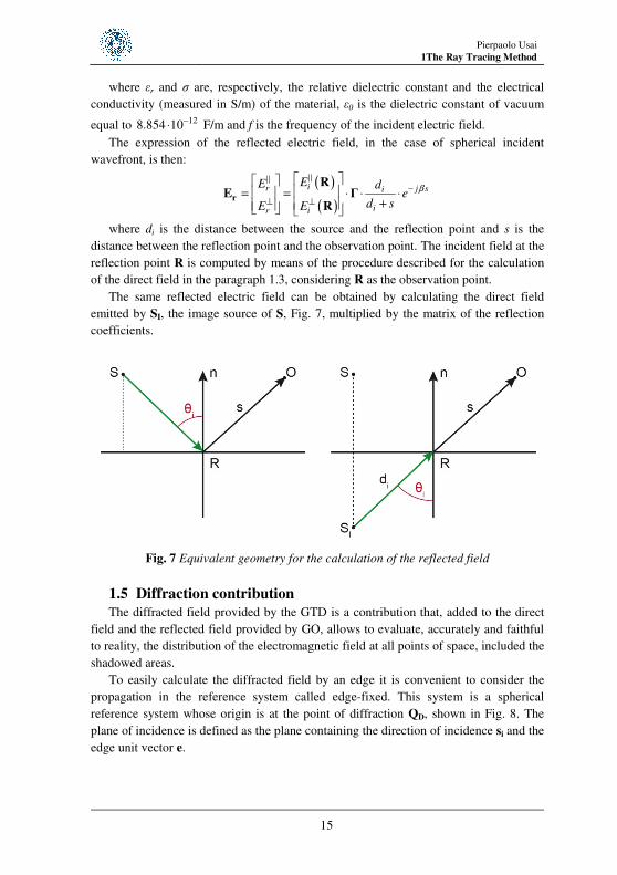
The expression of the reflected electric field, in the case of spherical incident
wavefront, is then:
( )
( )−
⊥ ⊥
= = ⋅ ⋅ ⋅
+ r
RE Γ
R
ir j si
ir i
EE de
d sE E
β
where di is the distance between the source and the reflection point and s is the
distance between the reflection point and the observation point. The incident field at the
reflection point R is computed by means of the procedure described for the calculation
of the direct field in the paragraph 1.3, considering R as the observation point.
The same reflected electric field can be obtained by calculating the direct field
emitted by SI, the image source of S, Fig. 7, multiplied by the matrix of the reflection
coefficients.
Fig. 7 Equivalent geometry for the calculation of the reflected field
1.5 Diffraction contribution
The diffracted field provided by the GTD is a contribution that, added to the direct
field and the reflected field provided by GO, allows to evaluate, accurately and faithful
to reality, the distribution of the electromagnetic field at all points of space, included the
shadowed areas.
To easily calculate the diffracted field by an edge it is convenient to consider the
propagation in the reference system called edge-fixed. This system is a spherical
reference system whose origin is at the point of diffraction QD, shown in Fig. 8. The
plane of incidence is defined as the plane containing the direction of incidence si and the
edge unit vector e.

Pierpaolo Usai
1 The Ray Tracing Method
16
Fig. 8 Edge-fixed reference system for the calculation of the diffracted field
The edge-fixed system is constituted by the unit vector si and the unit vectors iφφφφ and
βi, respectively, perpendicular and parallel to the plane of incidence which are given by
the following expressions
,− ×
= = ××
ii i i i
i
e ss
e sφ β φφ β φφ β φφ β φ .
From the diffraction point are originated infinite rays, which define the lateral
surface of a cone, called Keller's cone, having vertex at QD and aperture angle θd equal
to θi. Among these rays the one that reaches the observation point O defines the unit
vector sd, i.e. the direction of propagation of the diffracted ray. Known sd, the other two
unit vectors of the edge-fixed system along which the diffracted field is decomposed,
are
,×
= = ××
dd d d d
d
e sβ s
e sφ φφ φφ φφ φ .
The components of the field along the unit vector ϕi and ϕd are called hard ('h')
whereas those along βi and βd are called soft ('s'). The diffracted electric field is
therefore given by the following expression [2]
( )( )
( )
( )
( ) ( )−
= = ⋅ ⋅ ⋅ +
D
d
D
QE D
Q
d i is s j s
d i ih h
E s Es e
E s E s s
βρ
ρ

Pierpaolo Usai 1The Ray Tracing Method
17
where s is the distance between the point of diffraction QD and the observation point
O, iρ is the radius of curvature of the incident wavefront (equal to the distance between
the source S and QD in the case of a spherical incident wavefront) and D is the matrix of
the diffraction coefficients. In the edge-fixed reference system the matrix D is
0
0
− =
− D
s
h
D
D
in which s
D and h
D are given by [2][3]
( ) ( ), 1 2 , 3 4, , ', , = + +Γ +s h i s hD L n D D D Dφ φ ϑ
where Γs e Γ
h are the Fresnel reflection coefficients on the facets of the edge and
the quantities D1 ÷ D4 are
( )( )
/4
1
'cot '
22 2 sin
−++ − −
= −
j
i
eD F La
nn
π π φ φβ φ φ
πβ θ,
( )( )
/ 4
2
'cot '
22 2 sin
−−
− − − = −
j
i
eD F La
nn
π π φ φβ φ φ
πβ θ,
( )( )
/ 4
3
'cot '
22 2 sin
−++ + −
= +
j
i
eD F La
nn
π π φ φβ φ φ
πβ θ,
( )( )
/ 4
4
'cot '
22 2 sin
−−− + −
= +
j
i
eD F La
nn
π π φ φβ φ φ
πβ θ.
The angles φ and 'φ are shown in Fig 16.9 and n is a parameter related to the
internal angle α of the edge, expressed in radians, by the following relation
2 −=n
π α
π.
In the (16.28) - (16.31) F[x] is the Fresnel function given by
[ ] ( )22 exp ,∞
= −∫jx
xF x j xe j dξ ξ
L is a parameter that, in the case of a spherical incident wavefront, is
2'sin
'=
+i
ssL
s sθ
and ( )± ±a δ is a function given by
( ) 2 22 cos
2
± ±± ± −
=
Na
π δδ
where '± = ±δ φ φ and
±N are the integers which satisfy the following equations
( )2 + ±− =nNπ δ π
( )2 − ±− = −nNπ δ π .
Pierpaolo Usai
1 The Ray Tracing Method
18
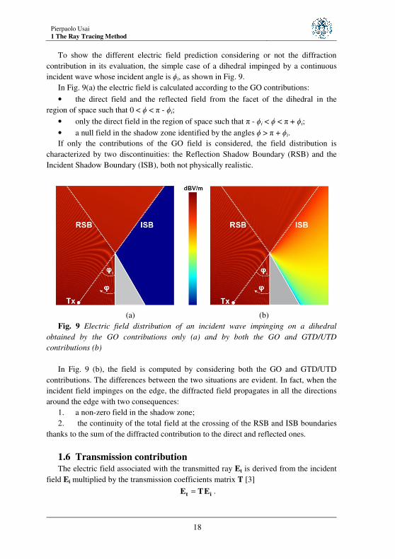
To show the different electric field prediction considering or not the diffraction
contribution in its evaluation, the simple case of a dihedral impinged by a continuous
incident wave whose incident angle is ϕi, as shown in Fig. 9.
In Fig. 9(a) the electric field is calculated according to the GO contributions:
• the direct field and the reflected field from the facet of the dihedral in the
region of space such that 0 < ϕ < π - ϕi;
• only the direct field in the region of space such that π - ϕi < ϕ < π + ϕi;
• a null field in the shadow zone identified by the angles ϕ > π + ϕi.
If only the contributions of the GO field is considered, the field distribution is
characterized by two discontinuities: the Reflection Shadow Boundary (RSB) and the
Incident Shadow Boundary (ISB), both not physically realistic.
(a) (b)
Fig. 9 Electric field distribution of an incident wave impinging on a dihedral
obtained by the GO contributions only (a) and by both the GO and GTD/UTD
contributions (b)
In Fig. 9 (b), the field is computed by considering both the GO and GTD/UTD
contributions. The differences between the two situations are evident. In fact, when the
incident field impinges on the edge, the diffracted field propagates in all the directions
around the edge with two consequences:
1. a non-zero field in the shadow zone;
2. the continuity of the total field at the crossing of the RSB and ISB boundaries
thanks to the sum of the diffracted contribution to the direct and reflected ones.
1.6 Transmission contribution
The electric field associated with the transmitted ray Et is derived from the incident
field Ei multiplied by the transmission coefficients matrix T [3]
=t iE TE .

Pierpaolo Usai 1The Ray Tracing Method
19
In the analysis of the outdoor wireless propagation by the ray tracing, the finite
thickness effects of the walls on the reflected field and the transmitted field evaluation
are neglected because strongly attenuated. On the contrary, in the indoor wireless
propagation analysis, it is necessary to take into account the wall thickness and the
multi-layered structure of walls (Fig. 10) in the calculation of the reflection and
transmission coefficients.
Fig. 10 Incident wave on a multi-layered wall
In this case the reflection and transmission coefficients of the entire multi-layered
structure can be obtained in an iterative way calculating the following quantities [4]
1, 1
1, 11
i
i
ji i i
i ji i i
r R eR
r R e
−+ −
−+ −
+=
+ +
δ
δ,
21, 1
1, 11
i
i
j
i i ii j
i i i
t T eT
r R e
−
+ −
−+ −
=+
δ
δ
0
4cos , i
i i i i i
i i
jn d
j= =
+
ωµπδ θ η
λ σ ωε
1 1 1 11, 1,
1 1 1 1
,cos cos cos cos
cos cos cos cosi i i ii i i i
i i i i
i i i ii i i i
r r+ + + ++ + ⊥
+ + + +
− + −= =
+ +
η θ η θ η θ η θ
η θ η θ η θ η θ
1 1
1 1 1 1
,2 cos 2 cos
cos cos cos cosi ii i
i i
i i i ii i i i
T T+ +⊥
+ + + +
= =+ +
η θ η θ
η θ η θ η θ η θ
where, for the i-th layer:
• di is the thickness,
• ni is the index of refraction,
• µi is the magnetic permeability,

Pierpaolo Usai
1 The Ray Tracing Method
20
• εi is the relative dielectric constant,
• σi is the electrical conductivity.
The relationship between the angles θi and θi+1 are derived by applying the Snell's
law:
( )1 1sin sin ,+ += = +i i i i i i i ij jγ θ γ θ γ ωµ σ ωε .
where γi is the propagation constant of the i-th layer.
The above formulation allows to iteratively evaluate the total reflection coefficient
RN and total transmission coefficient TN produced from a structure consisting of N layers
of different material.
Pierpaolo Usai 2 Arbitrary Voxel Selection
21
2 Arbitrary Voxel Selection
A method for speeding up a ray tracing based
electric field prediction model in urban environments.
In the Ray Tracing (RT) approach, buildings and terrain are geometrically modeled
by means of polygonal plane facets. The time required by the RT algorithm to compute
all rays connecting Txs and Rxs exponentially rises as the number of facets linearly
increases [5]. Therefore the physical coherence of the deterministic approach leads to a
boost of the computational time and this propagation model is thus often considered
time expensive if compared to the empirical and statistical ones.
In order to reduce the computational time and the memory requirement many
solutions have been proposed over the last decades, also in the field of visualization
applications. When the RT is based on an inverse algorithm, the visibility conditions
between each couple of facets play an important role in the computation time reduction
since it minimizes the number of times the visibility test routines are applied. For this
reason many techniques addressing this aspect are based on the visibility conditions
optimization. They split the space seen from a point in angular or axis-aligned regions
and store the facets of the model in the regions where they belong. For example,
Angular Z-Buffer (AZB), Space Volumetric Partitioning (SVP), Occluder Fusion, and
Binary Space Partitioning (BSP), have received great attention [5]-[7]. Because they act
only by speeding up geometrical checks, they do not introduce any approximation in the
field prediction compared with the full 3D RT analysis.
Another approach is the hybrid imaging technique [8], where the 3D paths research
starts from 2D image generations in horizontal and vertical planes. Another method [9]
combines horizontal 2D RT and knife-edge diffraction model to take into account the
street canyon effect and the radio propagation above rooftop. In [10] a method based on
a data base preprocessing is presented. The facets and edges are divided into tiles and
segments and the possible rays between them are computed and stored in a file. When

Pierpaolo Usai
2 Arbitrary Voxel Selection
22
the scene database remains the same and the Tx moves into the scene, this method
shows its best results, since the data stored in the file prevents to analyze again the
scenario. A 2D model that simplifies the real scenario by considering only the
horizontal 2D propagation mode between infinitely tall buildings is described in [11].
Recently, it has been proposed a simplification based on a heuristic preprocessing of
the scenario database [12]. This technique, given the Tx and Rx positions, identifies the
active part of the scene database selecting all buildings located within an ellipse of
focuses Tx and Rx, and in line of sight with the Tx and/or Rx. However, when the
distance between Tx and Rx and the largest scene dimension are comparable in order of
magnitude, the ellipse surface almost overlies the whole scenario and the method
becomes inefficient. To overcome this drawback due to an intrinsic geometric limit, in
this thesis, it is proposed a pre-processing refinement of the scene characterized by a
higher degree of flexibility of the selected area that will be subsequently analysed by the
RT method. By using a grid space division, a minimum area, based on the line
connecting Tx and Rx, is selected and it can also be refined or modified by the user.
This approach has been implemented on a ray tracer [7] which employs an inverse
3D deterministic RT algorithm, based on the image method, to simulate the
electromagnetic propagation in complex environments. Fixed k as the order of
simulation, the code engine is able to find all rays formed by sequences of up to k
elementary contributions including reflections and diffractions. A particular emphasis
will be given to the employment of our strategy for propagation in urban scenarios since
it is of paramount importance in the research field and in many applications such as
localization schemes [13], channel modeling [14][15], electromagnetic mapping in
urban areas [16]-[19].

Pierpaolo Usai 2 Arbitrary Voxel Selection
23
2.1 Algorithm description
In the first step a bounding box containing all the buildings in the scene is defined
and then a uniform adaptive grid [20] is locally applied. As shown in Fig. 11, the space
is divided into a set of Nv cells called voxels, an abbreviation of elemental volumes in
analogy to pixels (picture elements).
The number of voxels Nv is estimated by
x y
v
x y
Dim DimN
Dist Dist
⋅=
⋅ (1)
where Dimx and Dimy are the grid dimensions along X and Y axes. The distance
between Tx and Rx along the X axis is Distx while the distance along Y axis is Disty
(Fig. 12).
The total number of voxels Nv is set to be within the interval [30,400] in order to
have a useful partitioning of the scenario.
A higher number of voxels would make cumbersome the arbitrary selection operated
by the user and would create voxels which are too small and hence useless. Moreover,
this upper bound of the interval is useful when the distance between Tx and Rx is
smaller than the diagonal Dd of the scenario since it allows a finer voxel discretization of
the investigated area. The lower bound is necessary to manage the case when the
distance between Tx and Rx and the diagonal Dd are comparable. If Nv in (1) is less or
more than the lower or the upper bound respectively, its value is set equal to the nearest
bound. If Tx and Rx are aligned along a reference axis, the value of Nv is set equal to the
upper bound.
Because the chosen voxel's footprint is the square shape, the number of subdivisions
along X and Y, Nx and Ny, are taken proportionally to the grid dimensions along X and
Y axes. Given the proportional factors
,
,
xx y
y
y
x y
x
DimDim Dim
Dim
DimDim Dim
Dim
β
γ
= >
= <
we obtain
2
2
y y y x y
v x y
x x x x y
N N N Dim DimN N N
N N N Dim Dim
β β
γ γ
⋅ ⋅ = ⋅ >= ⋅ =
⋅ ⋅ = ⋅ <
and

Pierpaolo Usai
2 Arbitrary Voxel Selection
24
, ,
.
, ,
v
y x y x y
vx y x x y
NN N N Dim Dim
NN N N Dim Dim
ββ
γγ
= = ⋅ >
= = ⋅ <
Fig. 11. The uniform grid divides into voxels the considered scenario.
Fig. 12. Visualization of the parameters for a scenario with a couple of Tx and Rx.
Pierpaolo Usai 2 Arbitrary Voxel Selection
25
If more than one Rx is present, the algorithm is applied on the nearest one to the Tx.
By means of a matrix structure the membership of facets to the voxel is stored. By using
a grid space division, a minimum area comprising all cells crossed by the line
connecting Tx and Rx is selected. Next, a further subset of cells can be included by the
user who refines or modifies the set of voxels considered. Finally, it is important to
underline that the RT engine will only search the rays which interact with facets
contained in the selected voxels.
2.2 The algorithm validation for a test-case urban scenario
The accuracy of the algorithm is tested by analyzing the scene shown in
Fig. 13. The scenario represents a 1.5 GHz communication microcell in a Tokyo
street grid [21] where a line of receivers Rxi is placed along the path CAD. The model
of the buildings uses a relative permittivity εr equal to 15 and a conductivity σ of 7 S/m.
The Tx antenna is a half-lambda dipole and the Rxi antennas are assumed
omnidirectional. The grid sizes and the evaluated number of rows and columns are
summarized in Table 1, where Minimum Dist stands for the Distx and Disty parameters
relative to the nearest Rx to the Tx.
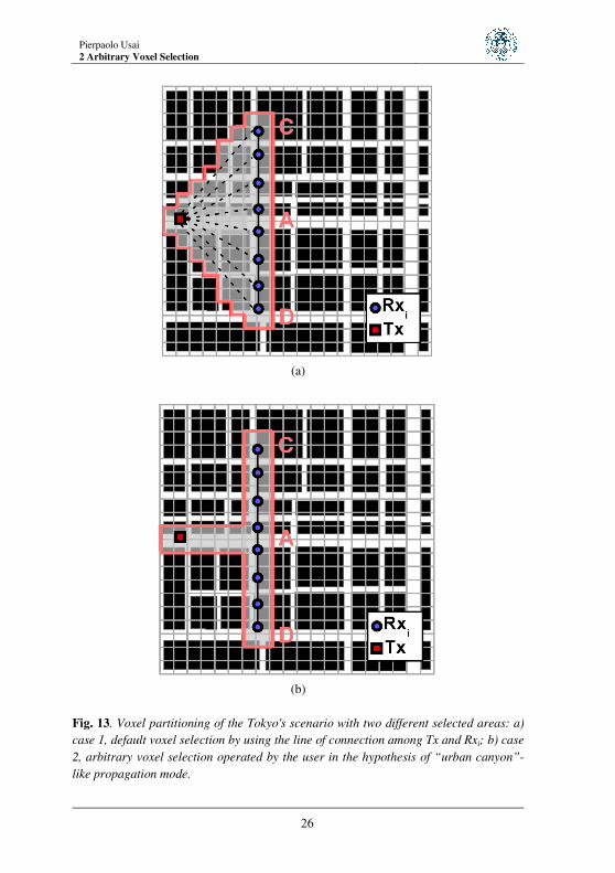
In order to show the flexibility and reliability of the proposed approach, two
different areas are considered for the analysis. The former (case 1) is enclosed by a
continuous red line in Fig. 3(a) and the gray area represents the default voxels’s
selection of the algorithm defined by the union of all the voxels crossed by the lines
connecting the Tx to each Rxi. The latter (case 2) is shown in Fig. 3(b) in the same way
as the former but the gray area represents an arbitrary finer selection operated by the
user. In fact a simple observation of the urban scenario under consideration suggest the
further reduction the user can operate. In the realistic hypothesis the height of the
buildings in an urban scenario is generally greater than Tx and Rx one, it can be inferred
that the propagation of the main contributions in terms of power delivered to the Rx will
take place in a “urban canyon”-like path which can be easily selected by removing some
voxels from the default grey area.
The measured data refer to the PL fluctuation along the line CAD and are taken
from [21].
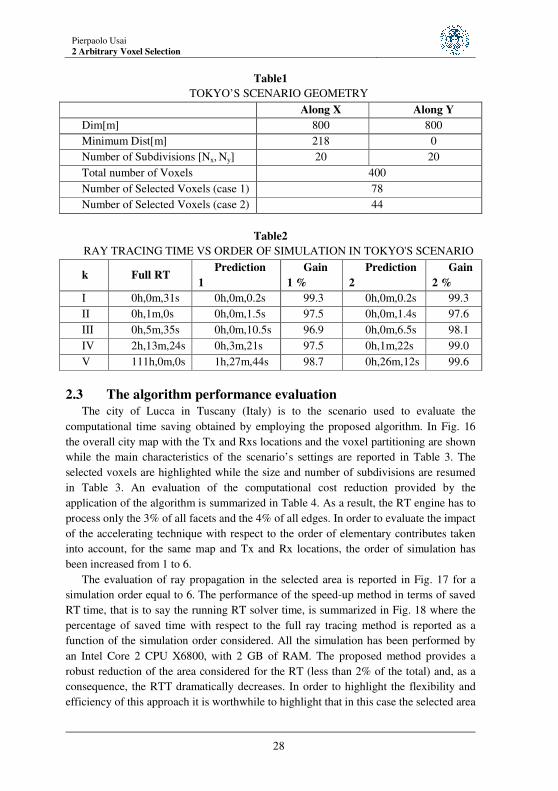
The analysis has been run with an order of simulation k = 5 for both case 1 and 2. A
Full RT analysis of the scene with the same order of simulation has been run too. A
satisfactory comparison of predicted and measured PL is shown in Fig. 14 and Fig. 15
and proves the accuracy of the estimate. Moreover it shows that no relevant
contributions are lost using both the two different areas as opposed to the Full RT
estimation. The improvements in terms of RT Time reduction are summed up in table 2
for both case1 and 2.
It is important to underline that a smart selection of the analyzed area can further
improve the acceleration as proven by the fact that the same PL prediction has been
obtained in both cases 1 and 2 but with a RT Time (RTT) reduction of about 70% in the
latter case where only 44 voxels are considered instead of 78.
Pierpaolo Usai
2 Arbitrary Voxel Selection
26
(a)
(b)
Fig. 13. Voxel partitioning of the Tokyo's scenario with two different selected areas: a)
case 1, default voxel selection by using the line of connection among Tx and Rxi; b) case
2, arbitrary voxel selection operated by the user in the hypothesis of “urban canyon”-
like propagation mode.

Pierpaolo Usai 2 Arbitrary Voxel Selection
27
-140
-130
-120
-110
-100
-90
-80
-70
-60
-300 -200 -100 0 100 200 300
MeasurementsFull RTPrediction 1
Path
Lo
ss
, [d
B]
Position along Y, [m]
Fig. 14. Comparison of the Path Loss estimations by the Full RT analysis and the
proposed algorithm.
-140
-130
-120
-110
-100
-90
-80
-70
-60
-300 -200 -100 0 100 200 300
MeasurementsPrediction 1Prediction 2
Pa
th L
oss
, [d
B]
Position along Y, [m]
Fig. 15. Comparison of the Path Loss estimations by two different applications of the
proposed algorithm.
Pierpaolo Usai
2 Arbitrary Voxel Selection
28
Table1
TOKYO’S SCENARIO GEOMETRY
Along X Along Y
Dim[m] 800 800
Minimum Dist[m] 218 0
Number of Subdivisions [Nx, Ny] 20 20
Total number of Voxels 400
Number of Selected Voxels (case 1) 78
Number of Selected Voxels (case 2) 44
Table2
RAY TRACING TIME VS ORDER OF SIMULATION IN TOKYO'S SCENARIO
k Full RT Prediction
1
Gain
1 %
Prediction
2
Gain
2 %
I 0h,0m,31s 0h,0m,0.2s 99.3 0h,0m,0.2s 99.3
II 0h,1m,0s 0h,0m,1.5s 97.5 0h,0m,1.4s 97.6
III 0h,5m,35s 0h,0m,10.5s 96.9 0h,0m,6.5s 98.1
IV 2h,13m,24s 0h,3m,21s 97.5 0h,1m,22s 99.0
V 111h,0m,0s 1h,27m,44s 98.7 0h,26m,12s 99.6
2.3 The algorithm performance evaluation
The city of Lucca in Tuscany (Italy) is to the scenario used to evaluate the
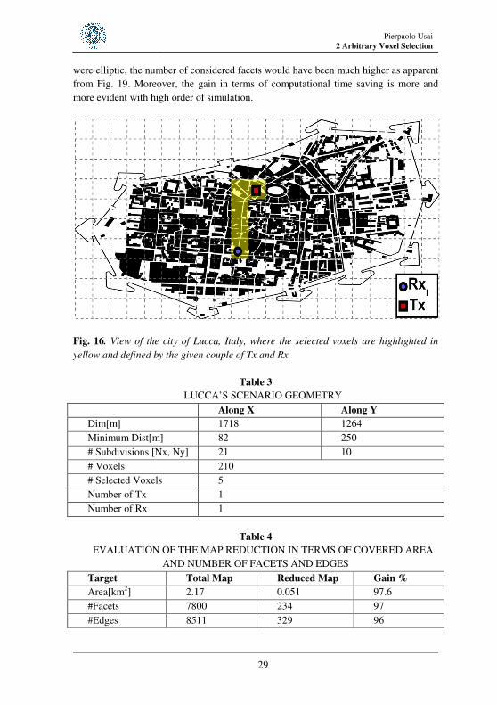
computational time saving obtained by employing the proposed algorithm. In Fig. 16
the overall city map with the Tx and Rxs locations and the voxel partitioning are shown
while the main characteristics of the scenario’s settings are reported in Table 3. The
selected voxels are highlighted while the size and number of subdivisions are resumed
in Table 3. An evaluation of the computational cost reduction provided by the
application of the algorithm is summarized in Table 4. As a result, the RT engine has to
process only the 3% of all facets and the 4% of all edges. In order to evaluate the impact
of the accelerating technique with respect to the order of elementary contributes taken
into account, for the same map and Tx and Rx locations, the order of simulation has
been increased from 1 to 6.
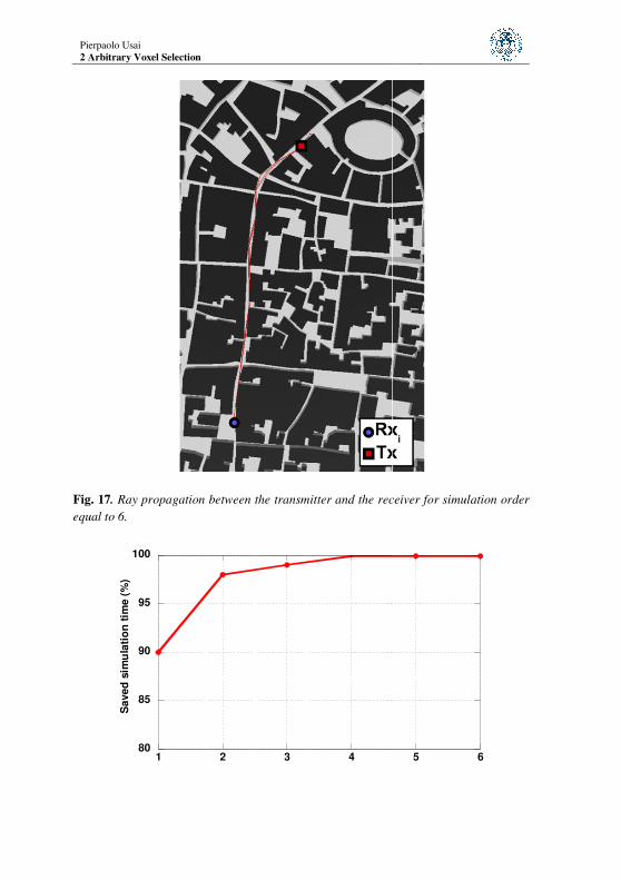
The evaluation of ray propagation in the selected area is reported in Fig. 17 for a
simulation order equal to 6. The performance of the speed-up method in terms of saved
RT time, that is to say the running RT solver time, is summarized in Fig. 18 where the
percentage of saved time with respect to the full ray tracing method is reported as a
function of the simulation order considered. All the simulation has been performed by
an Intel Core 2 CPU X6800, with 2 GB of RAM. The proposed method provides a
robust reduction of the area considered for the RT (less than 2% of the total) and, as a
consequence, the RTT dramatically decreases. In order to highlight the flexibility and
efficiency of this approach it is worthwhile to highlight that in this case the selected area
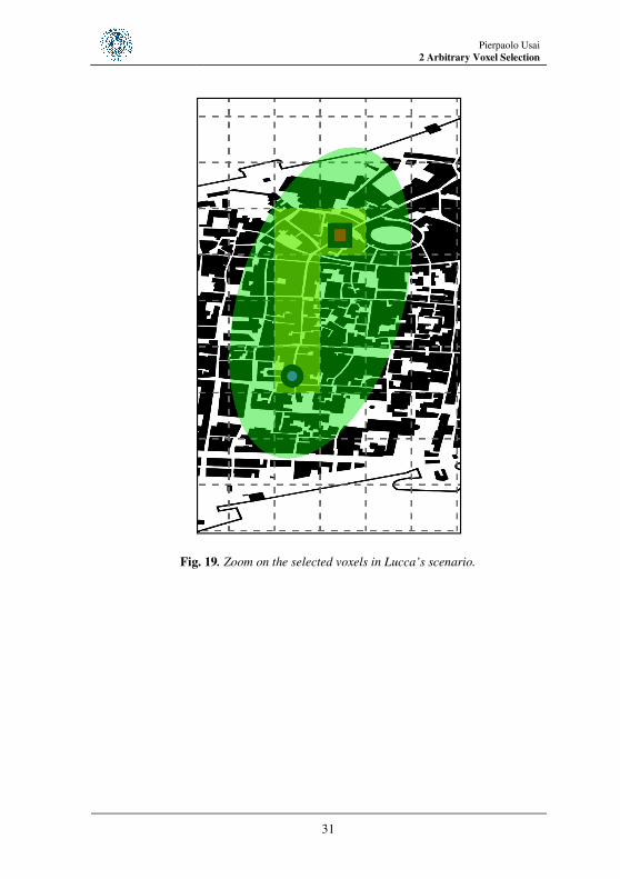
Pierpaolo Usai 2 Arbitrary Voxel Selection
29
were elliptic, the number of considered facets would have been much higher as apparent
from Fig. 19. Moreover, the gain in terms of computational time saving is more and
more evident with high order of simulation.
Fig. 16. View of the city of Lucca, Italy, where the selected voxels are highlighted in
yellow and defined by the given couple of Tx and Rx
Table 3
LUCCA’S SCENARIO GEOMETRY
Along X Along Y
Dim[m] 1718 1264
Minimum Dist[m] 82 250
# Subdivisions [Nx, Ny] 21 10
# Voxels 210
# Selected Voxels 5
Number of Tx 1
Number of Rx 1
Table 4
EVALUATION OF THE MAP REDUCTION IN TERMS OF COVERED AREA
AND NUMBER OF FACETS AND EDGES
Target Total Map Reduced Map Gain %
Area[km2] 2.17 0.051 97.6
#Facets 7800 234 97
#Edges 8511 329 96
Pierpaolo Usai
2 Arbitrary Voxel Selection
Fig. 17. Ray propagation between the transmitter and the receiver for simulation order
equal to 6.
80
85
90
95
100
1 2 3 4
Sa
ve
d s
imu
lati
on
tim
e (
%)
Order #
Ray propagation between the transmitter and the receiver for simulation order
5 6
Pierpaolo Usai 2 Arbitrary Voxel Selection
31
Fig. 19. Zoom on the selected voxels in Lucca’s scenario.

Pierpaolo Usai
2 Arbitrary Voxel Selection
32
Pierpaolo Usai 3 Channel Characterization by a Ray Tracing Analysis
33
3 Channel Characterization by
a Ray Tracing Analysis
Definition of the frequency response of a
communication channel by a ray tracing based
prediction model: impulse response and spreading
function estimation.
The communication channel of a wireless system operating in an outdoor or indoor
environment is characterized by the knowledge of the relation between the received
signal, or wireless system output, and that radiated from the source, or wireless system
input. This relationship varies with the operative frequency used, given the scenario and
the Tx and Rx settings. If the communication channel is a linear and time invariant
system, it can be characterized by the estimation of the frequency response. The ray
tracing analysis is an efficient method to evaluate the frequency response in scenarios
where the objects ‘size are greater than some wavelengths at high frequency respect to
with the full wave methods, [22]. Then, the impulse response of the channel is obtained
by means of the Fourier transform of the frequency response. In this way, the
communication channel can be modeled both in the frequency and delay domain.
If the scenario objects and antennas have zero speed, the multipath connecting Tx
and Rx does not change over time. So, fixed source and receiver, the paths that bounce
in the scenario are evaluated only once, and the electric field at the receiver is computed
in a post-processing phase by cycling in the frequency band. The ray tracing burden is
taken only once.
If the Rx moves in the scene, the channel link should be characterized by the
spreading function. Known the impulse response at each point of the Rx path, the
spreading function is computed by the Fourier transform respect to the time of the
impulse response.
Pierpaolo Usai
3 Channel Characterization by a Ray Tracing Analysis
34
3.1 Frequency response
Let us consider a time harmonic source 0exp( 2 )j fπ τ , at an arbitrary observation
point 0r . The time harmonic field at a fixed
0r observation point is given by
0 0 0 0 0 0 0 0
1
( , , ) ( , ) exp( 2 ) ( , ) exp( 2 )RAY
N
T i
i
E r f E r f j f E r f j fτ π τ π τ=
= =
∑ ,
where ( , )0 0E r fi is the field of the ith ray in the multipath link between Tx and Rx
evaluated by the RT algorithm, [23][22]. The dependence of the modulus and phase of
the field on the 0f frequency has been explicitly shown in the previous formula. For
each ray field contribution this dependence can be developed as
0 0 0 0 0 0 0 0 0 0( , ) ( , ) exp( 2 ) ( , )exp( 2 )ii i i i
dE r f E r f j f E r f j f
cπ π τ= − = −
where c is the speed of the light, di the length of the ith ray, and 0 0 0( , )iE r f is a complex
function that depends on the antenna gains, on the geometry and on the reflection or
diffraction coefficient.
If we consider the channel to be a linear and time invariant system in , the frequency
response of the channel at the 0f frequency can be expressed as
0 0 0 00 0 0 0
0 1
( , ) ( , )( , ) ( , )
1( )
RAYN
T Ti
i
E r f E r fH r f E r f
S f =
= = = ∑ɺ
where 0( )S fɺ is the phasor of the time harmonic source 0exp( 2 )j fπ τ .
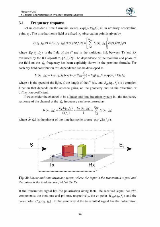
Fig. 20 Linear and time invariant system where the input is the transmitted signal and
the output is the total electric field at the Rx.
If the transmitted signal has the polarization along theta, the received signal has two
components: the theta one and phi one, respectively, the co-polar 0 0( , )H r fϑϑ and the
cross polar 0 0( , )H r fϑϕ . In the same way if the transmitted signal has the polarization
Pierpaolo Usai 3 Channel Characterization by a Ray Tracing Analysis
35
along phi, the received signal has two components: the theta one and the phi one,
respectively, the cross polar 0 0( , )H r fϕϑ and the polar 0 0( , )H r fϕϕ .
3.1.1 Narrow band signal
Let us consider a transmitted signal of bandwidth 2B at the carrier frequency cf . If
0 0( , )iE r f varies slowly in the proximity of the carrier frequency cf , it can be assumed
that
0 0 0 0( , ) ( , )i i cE r f E r f≅
0 0 0 0 0 01
( , ) ( , ) 2 ( ) ( , )2
c
i i c c i
f f
dE r f E r f j f f E r f
dfπ
π=
∠ ≅ ∠ + − ∠
and
0 0 0 0 0
0 0 0 0
( , ) ( , ) exp( ( , ) 2 )
( , ) exp( 2 ( ))
i i i i
i c i i c
E r f E r f j E r f j f
E r f j j f f
π τ
τ π
= ∠ − ≅
= − Φ − −
0 0 0( , ) 2i i c c iE r f fπ τΦ = −∠ + ,
0 0 01
( , )2
c
i i i
f f
dE r f
dfτ τ
π=
= − ∠ + ,
dii
cτ =
where [ , ]c cf f B f B∈ − + .
In most cases the phase slope 0 01
( , )2
c
i
f f
dE r f
dfπ=
− ∠ , due to the antenna gains, to
the geometry and to the reflection or diffraction coefficient, is quite small so that we can
assume 0i iτ τ≅ .
If we consider the channel to be a linear and time invariant system, the frequency
response of the channel, can be expressed as
00 0 0 0 0
0 0 0 0
0 0 0 0 0
( , )( , ) ( , ) ( , ) exp( )exp( 2 ( ))
( )
( , ) exp( ( , ) 2 )exp( 2 ( ) )
( , ) exp( ( , )) exp( 2 ) ( , )exp( 2 )
Ti i c i i c
c i i
i c i c c i c i
i
i c i c i i c i
i i
E r fH r f E r f E r f j j f f
S f
E r f j E r f j f j f f
E r f j E r f j f a r f j f
τ π
π τ π τ
π τ π τ
= = ≅ − Φ − − =
= ∠ − − − =
= ∠ − = −
∑ ∑
∑
∑ ∑
ɺ
where [ , ]c cf f B f B∈ − + .
In the hypothesis of narrow band source signal it is enough to estimate the electric
field of each ray at the carrier frequency cf in order to compute the transfer function in
a 2B band around the carrier frequency cf .
Pierpaolo Usai
3 Channel Characterization by a Ray Tracing Analysis
36
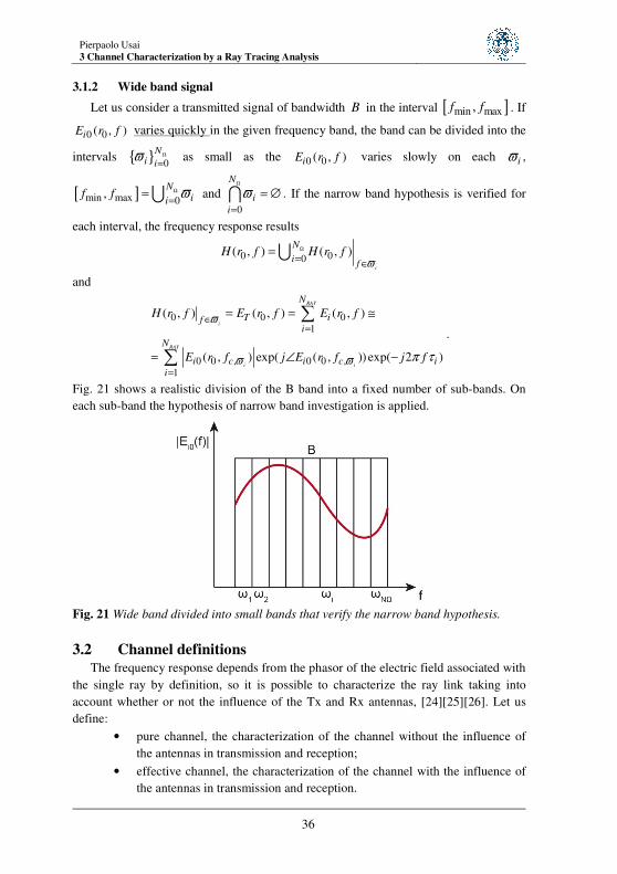
3.1.2 Wide band signal
Let us consider a transmitted signal of bandwidth B in the interval [ ]min max,f f . If
0 0( , )iE r f varies quickly in the given frequency band, the band can be divided into the
intervals 0
Ni i
ϖ Ω
= as small as the 0 0( , )iE r f varies slowly on each iϖ ,
[ ]min max 0,
Nii
f f ϖΩ
==∪ and
0
N
i
i
ϖΩ
=
= ∅∩ . If the narrow band hypothesis is verified for
each interval, the frequency response results
0 00( , ) ( , )
i
N
if
H r f H r fϖ
Ω
= ∈=∪
and
0 0 01
0 0 , 0 0 ,
1
( , ) ( , ) ( , )
( , ) exp( ( , )) exp( 2 )
RAY
i
RAY
i i
N
T ifi
N
i c i c i
i
H r f E r f E r f
E r f j E r f j f
ϖ
ϖ ϖ π τ
∈=
=
= = ≅
= ∠ −
∑
∑
.
Fig. 21 shows a realistic division of the B band into a fixed number of sub-bands. On
each sub-band the hypothesis of narrow band investigation is applied.
Fig. 21 Wide band divided into small bands that verify the narrow band hypothesis.
3.2 Channel definitions
The frequency response depends from the phasor of the electric field associated with
the single ray by definition, so it is possible to characterize the ray link taking into
account whether or not the influence of the Tx and Rx antennas, [24][25][26]. Let us
define:
• pure channel, the characterization of the channel without the influence of
the antennas in transmission and reception;
• effective channel, the characterization of the channel with the influence of
the antennas in transmission and reception.
Pierpaolo Usai 3 Channel Characterization by a Ray Tracing Analysis
37
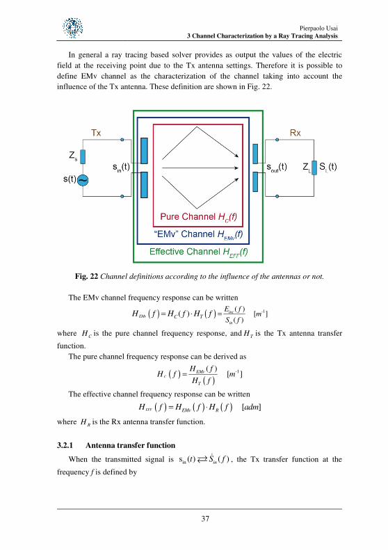
In general a ray tracing based solver provides as output the values of the electric
field at the receiving point due to the Tx antenna settings. Therefore it is possible to
define EMv channel as the characterization of the channel taking into account the
influence of the Tx antenna. These definition are shown in Fig. 22.
Fig. 22 Channel definitions according to the influence of the antennas or not.
The EMv channel frequency response can be written
( ) ( ) -1( ) [ ]
( )( )EMv
inc
in
TC
E fm
S fH f H f H f == ⋅
where C
H is the pure channel frequency response, andT
H is the Tx antenna transfer
function.
The pure channel frequency response can be derived as
( )( )
-1( ) [ ]C
EMv
T
H fH f m
H f=
The effective channel frequency response can be written
( ) ( ) ( ) [ ]EFF EMv RH f H f H f adm= ⋅
where RH is the Rx antenna transfer function.
3.2.1 Antenna transfer function
When the transmitted signal is ins ( ) ( )int S fɺ , the Tx transfer function at the
frequency f is defined by
Pierpaolo Usai
3 Channel Characterization by a Ray Tracing Analysis
38
( )( )
( ) [ ]
FF jkR
T
in
E PH f R e adm
S f⋅
ɺ≜ɺ
where ( )FFE Pɺ is the electric field phasor in the receiver point FFP at the distance R in
the far field of the transmitter antenna. That is, ( )FFE P equals the free space direct ray
contribution between Tx and Rx.
By the reciprocity theorem the transfer function of the Rx antenna is computed by
( )( )
( )( )0 [ ]
out
R Tinc
S f cH f H f m
j fE RX= ⋅
⋅
ɺ≜ ɺ
where ( )outS fɺ is the received voltage phasor, ( )inc
E RXɺ the incident electric field
phasor at the receiver point and 0
c the light speed in the vacuum. The easier way to
compute ( )RH f is by the evaluation of the ( )TH f .
Both the transfer functions, ( )TH f and ( )RH f , have to be evaluated once the ray is
fixed, i.e., they depend on the ray angle of departure and arrival, respectively. So, for
each frequency, there exist as many values of the antennas transfer functions as the
possible ray orientations at the Tx and Rx locations, respectively. The definition of the
antenna transfer function is easily to know only for few types of antennas. For example,
the half wavelength dipole transfer function is related to with its effective length
function. When the antennas do not have an analytical model able to predict its behavior
in the considered bandwidth, a full-wave analysis of the antennas structure and feeder
has to be conducted.
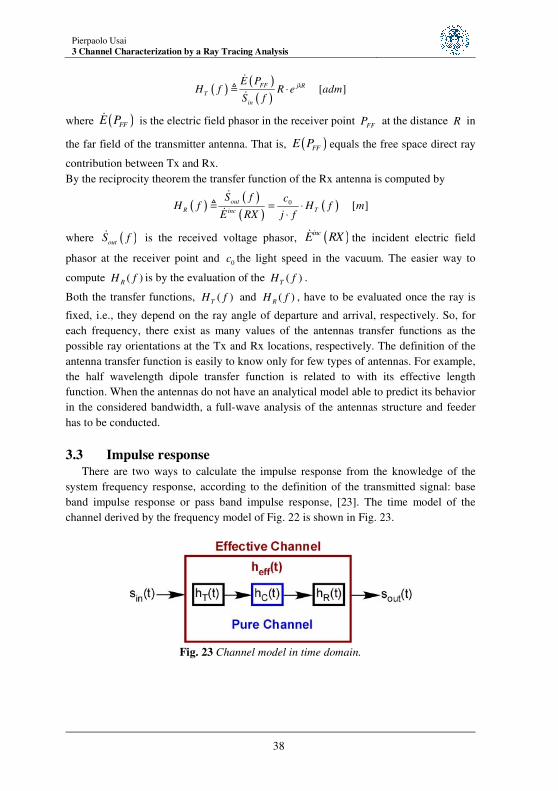
3.3 Impulse response
There are two ways to calculate the impulse response from the knowledge of the
system frequency response, according to the definition of the transmitted signal: base
band impulse response or pass band impulse response, [23]. The time model of the
channel derived by the frequency model of Fig. 22 is shown in Fig. 23.
Fig. 23 Channel model in time domain.
Pierpaolo Usai 3 Channel Characterization by a Ray Tracing Analysis
39
3.3.1 Base band system
Known the frequency response 0( , )H r f in the band min max2 [ , ]B f f= at an
arbitrary observation point 0r of a base-band system, the impulse response can be
evaluated by means of the Inverse Fourier Transform (IFT) of the frequency response as
max
min
0 0 0
0
0 02
0 02 2
( , ) ( ( , )) ( , ) exp( 2 )
( , ) exp( 2 ) ( , ) exp( 2 )
Re[ ( , ) exp( 2 )] Im[ ( , ) exp( 2 )]
f
f Bf
f B f B
h r IFT H r f H r f j f df
H r f j f df H r f j f f
H r f j f f j H r f j f f
τ π τ
π τ π τ
π τ π τ
∆
∆ ∆
∞
∆ ∆∈
∆ ∆ ∆ ∆∈ ∈
= = =
= ≅ ∆ =
= ∆ + ∆
∫
∑∫
∑ ∑
where min max , 1, 2,3,...,2
f f Bf m f m
f∆
+ = ± ∆ = ∆
and f∆ is the sampling frequency
step.
3.3.2 Pass band system
The impulse response of a pass-band system can be written as
0 0 0 0( , ) ( , ) cos(2 ) ( , ) sin(2 ) Re[ ( , ) exp( 2 )]
I c Q c c ch r h r f h r f h r j fτ τ π τ τ π τ τ π τ= − =
where its complex envelope is given by the following expression
0 0 0( , ) ( , ) ( , )c I Qh r h r jh rτ τ τ= + .
The relationship between the frequency response of the pass-band system and the
frequency response of the in–phase and in-quadrature components as
0 0
0
0 0
1( , ) ( , ) 0
2 2( , )
1( , ) ( , ) 0
2 2
I c Q c
I c Q c
jH r f f H r f f f
H r fj
H r f f H r f f f
− + − ≥
= + − + ≤
.
By reversing the above relationship it is obtained
0 0 0
0 0 0
( , ) ( , ) ( , )
( , ) ( , ) ( , )
I c c
Q c c
H r f H r f f H r f f
H r f jH r f f jH r f f
+ −
+ −
= + + −
= − + + −
where
0 0
0 0
( , ) ( , ) ( )
( , ) ( , ) ( )
H r f H r f u f
H r f H r f u f
+
−
=
= − and
1 if 0( )
0 if < 0
fu f
f
≥=
.
The in-phase and in-quadrature impulse response components are computed by the
inverse Fourier transform of the 0( , )IH r f and
0( , )
QH r f , respectively:

Pierpaolo Usai
3 Channel Characterization by a Ray Tracing Analysis
40
0
2
0
0
2
1( , )exp( 2 ( ) ) 0
2( , )
1( , ) exp( 2 ( ) ) 0
2
K
K
K K c
f B
I
K K c
f B
H r f j f f f f
h r
H r f j f f f f
π
π
∈
∈
+ τ ∆ ≤
τ =
− τ ∆ ≥
∑
∑
0
2
0
0
2
1( , ) exp( 2 ( ) ) 0
2( , )
1( , ) exp( 2 ( ) ) 0
2
K
K
K K c
f B
Q
K K c
f B
j H r f j f f f f
h r
j H r f j f f f f
π
π
∈
∈
+ τ ∆ ≤
τ =
− − τ ∆ ≥
∑
∑
where , 1, 2,3,...,K c
Bf f m f m
f= ± ∆ =
∆, B is the bandwidth and f∆ is the sampling
frequency step.
3.3.3 Power Delay Profile and Delay Spread evaluation
The Power Delay Profile-PDP and the Delay Spread-DS are two parameters
characterizing the wireless communication channel that can be directly evaluated by the
impulse response.
The PDP describes the power distribution in the delay domain and is evaluated
referring to a Tx-Rx link as 2
0 0( , ) ( , )PDP r h rτ τ= .
The spatial average PDP can be calculated averaging the PDPs at each Rx point as
2
1
1( ) ( , )
RXN
avr i
iRX
PDP h rN
τ τ=
= ∑ .
The average delay avr
τ and delay spread rms
τ are evaluated as
( )avr tP t dtτ = ∫
2( ) ( )
rms avrt P t dtτ = − τ∫
( ) ( ) / ( )P PDP PDP t dtτ = τ ∫
where ( )P τ is the normalized PDP function.
3.4 Spreading function
The spreading function ( , )DSF f τ is evaluated as the Fourier transform (FT) with
respect to time of the impulse response
Pierpaolo Usai 3 Channel Characterization by a Ray Tracing Analysis
41
( , ) ( ( , )) ( (O( ), )) (O( ), )exp( 2 )D DSF f FT h t FT h t h t j f t dtτ τ τ τ π∞
−∞
= = = − =∫
000
(O( ), )exp( 2 ) ( , )exp( 2 )
Obs
Obs
TT t
D n D
n
h t j f t dt h r j f n t tτ π τ π∆
=
= − ≅ − ∆ ∆∑∫
where t determines the relative position O(t) of the receiver with respect to the
transmitter, according to the considered law of motion. The power spectrum in the
domain of the delays and the Doppler frequency shift is evaluated as |SF(fD,τ)|2.
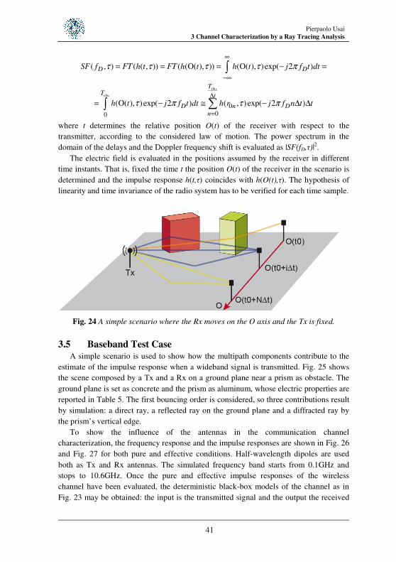
The electric field is evaluated in the positions assumed by the receiver in different
time instants. That is, fixed the time t the position O(t) of the receiver in the scenario is
determined and the impulse response h(t,τ) coincides with h(O(t),τ). The hypothesis of
linearity and time invariance of the radio system has to be verified for each time sample.
Fig. 24 A simple scenario where the Rx moves on the O axis and the Tx is fixed.
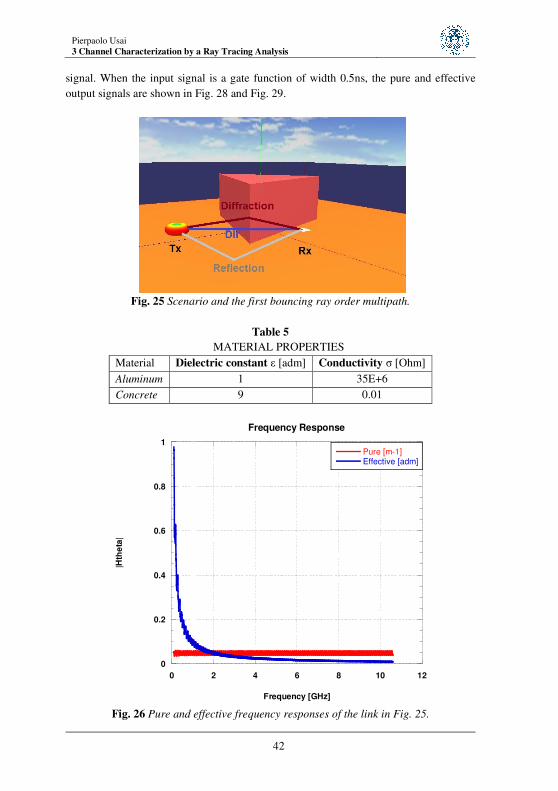
3.5 Baseband Test Case
A simple scenario is used to show how the multipath components contribute to the
estimate of the impulse response when a wideband signal is transmitted. Fig. 25 shows
the scene composed by a Tx and a Rx on a ground plane near a prism as obstacle. The
ground plane is set as concrete and the prism as aluminum, whose electric properties are
reported in Table 5. The first bouncing order is considered, so three contributions result
by simulation: a direct ray, a reflected ray on the ground plane and a diffracted ray by
the prism’s vertical edge.
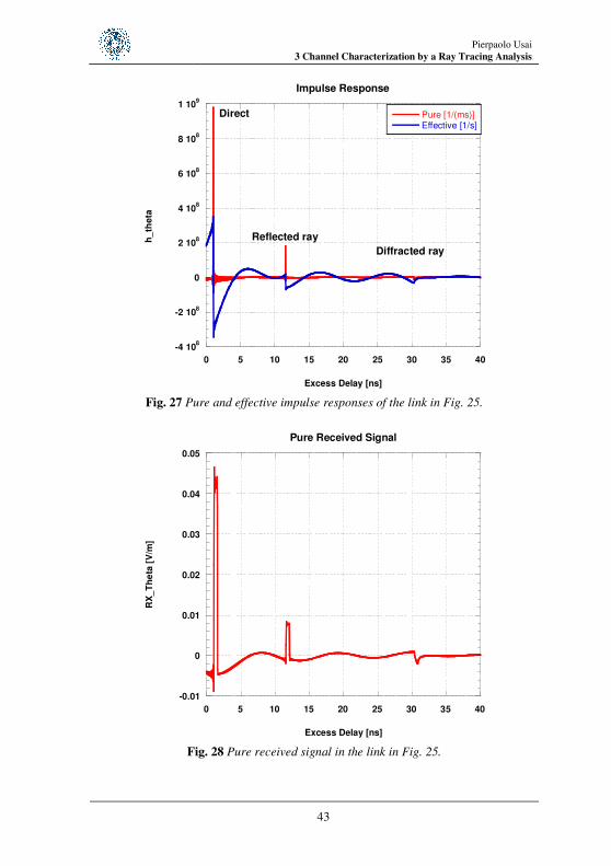
To show the influence of the antennas in the communication channel
characterization, the frequency response and the impulse responses are shown in Fig. 26
and Fig. 27 for both pure and effective conditions. Half-wavelength dipoles are used
both as Tx and Rx antennas. The simulated frequency band starts from 0.1GHz and
stops to 10.6GHz. Once the pure and effective impulse responses of the wireless
channel have been evaluated, the deterministic black-box models of the channel as in
Fig. 23 may be obtained: the input is the transmitted signal and the output the received
Pierpaolo Usai
3 Channel Characterization by a Ray Tracing Analysis
42
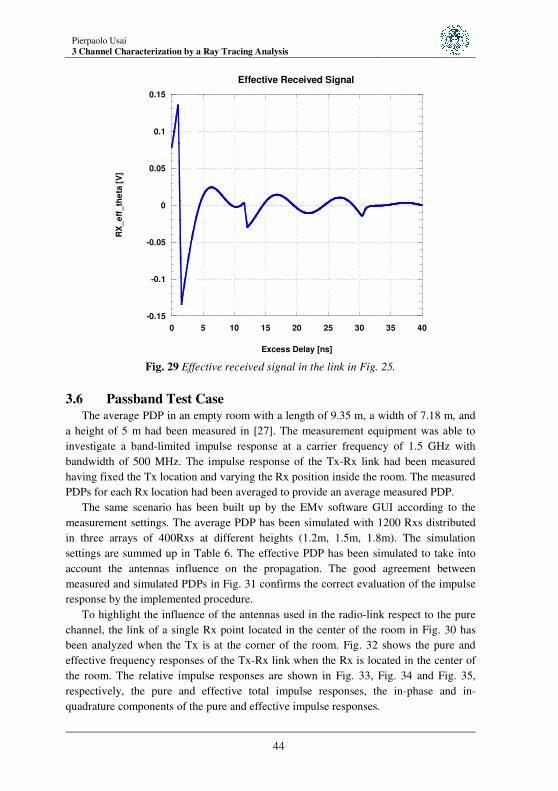
signal. When the input signal is a gate function of width 0.5ns, the pure and effective
output signals are shown in Fig. 28 and Fig. 29.
Fig. 25 Scenario and the first bouncing ray order multipath.
Table 5
MATERIAL PROPERTIES
Material Dielectric constant ε [adm] Conductivity σ [Ohm]
Aluminum 1 35E+6
Concrete 9 0.01
0
0.2
0.4
0.6
0.8
1
0 2 4 6 8 10 12
Frequency Response
Pure [m-1]Effective [adm]
|Hth
eta
|
Frequency [GHz]
Fig. 26 Pure and effective frequency responses of the link in Fig. 25.
Pierpaolo Usai 3 Channel Characterization by a Ray Tracing Analysis
43
-4 108
-2 108
0
2 108
4 108
6 108
8 108
1 109
0 5 10 15 20 25 30 35 40
Impulse Response
Pure [1/(ms)]Effective [1/s]
h_th
eta
Excess Delay [ns]
Direct
Reflected ray
Diffracted ray
Fig. 27 Pure and effective impulse responses of the link in Fig. 25.
-0.01
0
0.01
0.02
0.03
0.04
0.05
0 5 10 15 20 25 30 35 40
Pure Received Signal
RX
_T
he
ta [
V/m
]
Excess Delay [ns]
Fig. 28 Pure received signal in the link in Fig. 25.
Pierpaolo Usai
3 Channel Characterization by a Ray Tracing Analysis
44
-0.15
-0.1
-0.05
0
0.05
0.1
0.15
0 5 10 15 20 25 30 35 40
Effective Received Signal
RX
_e
ff_th
eta
[V
]
Excess Delay [ns]
Fig. 29 Effective received signal in the link in Fig. 25.
3.6 Passband Test Case
The average PDP in an empty room with a length of 9.35 m, a width of 7.18 m, and
a height of 5 m had been measured in [27]. The measurement equipment was able to
investigate a band-limited impulse response at a carrier frequency of 1.5 GHz with
bandwidth of 500 MHz. The impulse response of the Tx-Rx link had been measured
having fixed the Tx location and varying the Rx position inside the room. The measured
PDPs for each Rx location had been averaged to provide an average measured PDP.
The same scenario has been built up by the EMv software GUI according to the
measurement settings. The average PDP has been simulated with 1200 Rxs distributed
in three arrays of 400Rxs at different heights (1.2m, 1.5m, 1.8m). The simulation
settings are summed up in Table 6. The effective PDP has been simulated to take into
account the antennas influence on the propagation. The good agreement between
measured and simulated PDPs in Fig. 31 confirms the correct evaluation of the impulse
response by the implemented procedure.
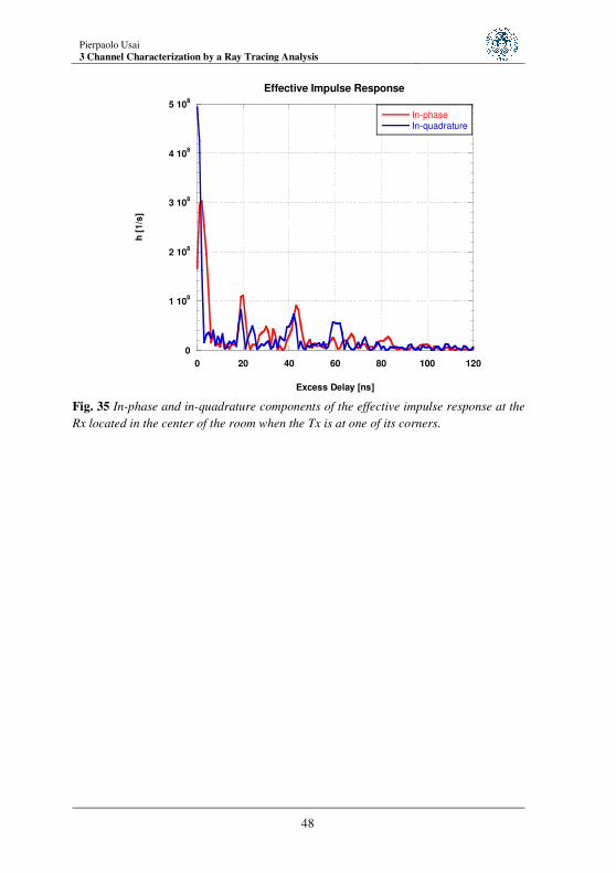
To highlight the influence of the antennas used in the radio-link respect to the pure
channel, the link of a single Rx point located in the center of the room in Fig. 30 has
been analyzed when the Tx is at the corner of the room. Fig. 32 shows the pure and
effective frequency responses of the Tx-Rx link when the Rx is located in the center of
the room. The relative impulse responses are shown in Fig. 33, Fig. 34 and Fig. 35,
respectively, the pure and effective total impulse responses, the in-phase and in-
quadrature components of the pure and effective impulse responses.

Pierpaolo Usai 3 Channel Characterization by a Ray Tracing Analysis
45
Table 6
SIMULATION SETTINGS
Ray bouncing order 5
Carrier frequency 1.5GHz
Bandwidth 0.5GHz
Number of frequency samples 126
Frequency step 4MHz
Tx and Rx Antennas Half wavelength dipoles
Fig. 30 The simulated room with a length of 9.35 m, a width of 7.18 m, and a height of
5.00 m with the fixed Tx position and three arrays of Rxs.

Pierpaolo Usai
3 Channel Characterization by a Ray Tracing Analysis
46
-35
-30
-25
-20
-15
-10
-5
0
5
0 20 40 60 80 100 120
PowerDelayProfile
SimulationMeasurement
PD
Pe
ff [
dB
]
Excess Delay [ns]
Fig. 31 The simulated and measured PDP in the scenario in Fig. 30
0
0.5
1
1.5
2
2.5
3
1.2 1.3 1.4 1.5 1.6 1.7 1.8
FrequencyResponse
Pure [1/m]Effective [adm]
|Hth
eta
|
Frequency [GHz]
Fig. 32 Pure and effective frequency responses at the Rx located in the center of the
room when the Tx is at one of its corners.

Pierpaolo Usai 3 Channel Characterization by a Ray Tracing Analysis
47
0
2 108
4 108
6 108
8 108
1 109
1.2 109
0 20 40 60 80 100 120
Total Impulse Response
Pure [1/(ms)]Effective [1/s]
hT
heta
Excess Delay [ns]
Fig. 33 Pure and effective impulse responses at the Rx located in the center of the room
when the Tx is at one of its corners.
0
2 107
4 107
6 107
8 107
1 108
0 20 40 60 80 100 120
Pure Impulse Response
In-phaseIn-quadrature
Excess Delay [ns]
h [
1/(
ms)]
Fig. 34 In-phase and in-quadrature components of the pure impulse response at the Rx
located in the center of the room when the Tx is at one of its corners.
Pierpaolo Usai
3 Channel Characterization by a Ray Tracing Analysis
48
0
1 108
2 108
3 108
4 108
5 108
0 20 40 60 80 100 120
Effective Impulse Response
In-phaseIn-quadrature
h [
1/s
]
Excess Delay [ns]
Fig. 35 In-phase and in-quadrature components of the effective impulse response at the
Rx located in the center of the room when the Tx is at one of its corners.

Pierpaolo Usai 4 Estimation of Airport Surface Propagation Channel
49
4 Estimation of Airport Surface
Propagation Channel
An evaluation of the surface propagation channel in
dynamic airport environments by using a ray tracing
technique.
New solutions for airport surface communications have been investigating since the
C band frequency interval between 5091-5150 MHz has been allocated to the
Aeronautical Mobile Route Service by the World Radio Conference in 2007. This new
frequency band allocation is due to the congestion of the previous VHF band between
118-137 MHz that is caused by the more and more growing needs of wider spectra for
continental domain communication systems.
The SANDRA project (Seamless Aeronautical Networking through integration of
Data links Radios and Antennas) is aimed at defining, integrating and validating
aeronautical communication architecture. The integration should be realized at different
levels: services, networks, radios and antennas. A technical profile and architecture for a
WiMAX based tower-aircraft communication system should be defined, designed and
validated.
Inside the SANDRA project, I had the opportunity to join with the task that
investigated the physical level. One of the target’s task was the estimation of the
channel model in order to evaluate the performance of the planned system.
Very few studies on the propagation modeling in big airport environments at the C
band have been conducted in the last decades and never before. A wideband statistical
channel characterization in the 5-GHz band around large airport surface areas is
presented in [28] while small size airports are analyzed in [29]. In both cases three
Pierpaolo Usai
4 Estimation of Airport Surface Propagation Channel
50
propagation regions are identified based upon different delay dispersion conditions and
for each region an empirical stochastic channel model is derived.
The proposed approach to characterize the airport surface channel is based on the
estimation of the radio wave propagation in the airport environments by the high
frequency methods: GO, GTD and UTD, [30], [31]. Starting from the reconstruction of
an environment, the algorithm of ray tracing allows the deterministic reconstruction of
paths made by the wave fronts to connect the transmitter to the receiver interacting with
objects present in the scene. Specifically, the international Munich airport has been
modeled as the German Aerospace Center (DLR) had conducted a measurement
campaign in different areas of this airport in 2007, [32], [33]. The paths estimation, in
terms of length (or delay), kind of contributions (direct, reflection and diffraction), and
angles of departure and arrival, allows the asymptotic method to estimate the following
parameters: electric and magnetic fields, and the received power, known the antennas
patterns. A typical airport scenario is composed by static and dynamic objects. In fact it
is composed by static buildings, terminals and operational infrastructures, and by
airplanes and vehicles moving in the apron or in the landing ramps. The channel
characterization of dynamic scenarios coincides with the estimate of the received power
distribution in the delay-Doppler domain, called Spreading Function (SF).
The canonical approach solving the estimate of the SF starts from the evaluation of
the frequency response of the channel and concludes by two consecutive Fourier
transforms of the frequency response: an inverse transform respect to the frequency
estimates the impulse response and its direct transform respect to the time provides the
SF. This approach is applicable in both wide and narrow band source signals and can be
used as a reference for other procedures.
An alternative approach is proposed. First, it evaluates the geometrical RT
information for all Tx-Rx pairs, then for each Rx power, delay and Doppler frequency
shift are computed. Finally, the Doppler delay power spectrum is obtained. This
approach avoids any Fourier transform and gives a deterministic evaluation of the
channel parameters. On the contrary the canonical approach starts from a deterministic
evaluation of the frequency response.
Both the procedures have been implemented in computer codes and used to test the
Munich Airport scenario by comparing their results with the measurement data.
Furthermore, the electromagnetic airport model was validated by comparing the
estimated power with the measured one along fixed routes inside the Munich airport
apron.
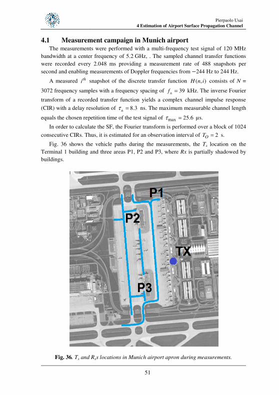
Pierpaolo Usai 4 Estimation of Airport Surface Propagation Channel
51
4.1 Measurement campaign in Munich airport
The measurements were performed with a multi-frequency test signal of 120 MHz
bandwidth at a center frequency of 5.2 GHz, . The sampled channel transfer functions
were recorded every 2.048 ms providing a measurement rate of 488 snapshots per
second and enabling measurements of Doppler frequencies from −244 Hz to 244 Hz.
A measured thi snapshot of the discrete transfer function ( , )H n i consists of N =
3072 frequency samples with a frequency spacing of 39f = kHz. The inverse Fourier
transform of a recorded transfer function yields a complex channel impulse response
(CIR) with a delay resolution of 8.3τ = ns. The maximum measurable channel length
equals the chosen repetition time of the test signal of max 25.6τ = µs.
In order to calculate the SF, the Fourier transform is performed over a block of 1024
consecutive CIRs. Thus, it is estimated for an observation interval of 2OT = s.
Fig. 36 shows the vehicle paths during the measurements, the Tx location on the
Terminal 1 building and three areas P1, P2 and P3, where Rx is partially shadowed by
buildings.
Fig. 36. Tx and Rxs locations in Munich airport apron during measurements.
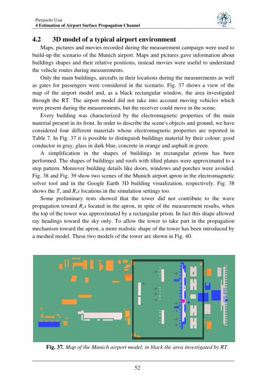
Pierpaolo Usai
4 Estimation of Airport Surface Propagation Channel
52
4.2 3D model of a typical airport environment
Maps, pictures and movies recorded during the measurement campaign were used to
build-up the scenario of the Munich airport. Maps and pictures gave information about
buildings shapes and their relative positions, instead movies were useful to understand
the vehicle routes during measurements.
Only the main buildings, aircrafts in their locations during the measurements as well
as gates for passengers were considered in the scenario. Fig. 37 shows a view of the
map of the airport model and, as a black rectangular window, the area investigated
through the RT. The airport model did not take into account moving vehicles which
were present during the measurements, but the receiver could move in the scene.
Every building was characterized by the electromagnetic properties of the main
material present in its front. In order to describe the scene's objects and ground, we have
considered four different materials whose electromagnetic properties are reported in
Table 7. In Fig. 37 it is possible to distinguish buildings material by their colour: good
conductor in gray, glass in dark blue, concrete in orange and asphalt in green.
A simplification in the shapes of buildings in rectangular prisms has been
performed. The shapes of buildings and roofs with tilted planes were approximated to a
step pattern. Moreover building details like doors, windows and porches were avoided.
Fig. 38 and Fig. 39 show two scenes of the Munich airport apron in the electromagnetic
solver tool and in the Google Earth 3D building visualization, respectively. Fig. 38
shows the Tx and Rxs locations in the simulation settings too.
Some preliminary tests showed that the tower did not contribute to the wave
propagation toward Rxs located in the apron, in spite of the measurement results, when
the top of the tower was approximated by a rectangular prism. In fact this shape allowed
ray headings toward the sky only. To allow the tower to take part in the propagation
mechanism toward the apron, a more realistic shape of the tower has been introduced by
a meshed model. These two models of the tower are shown in Fig. 40.
Fig. 37. Map of the Munich airport model, in black the area investigated by RT.
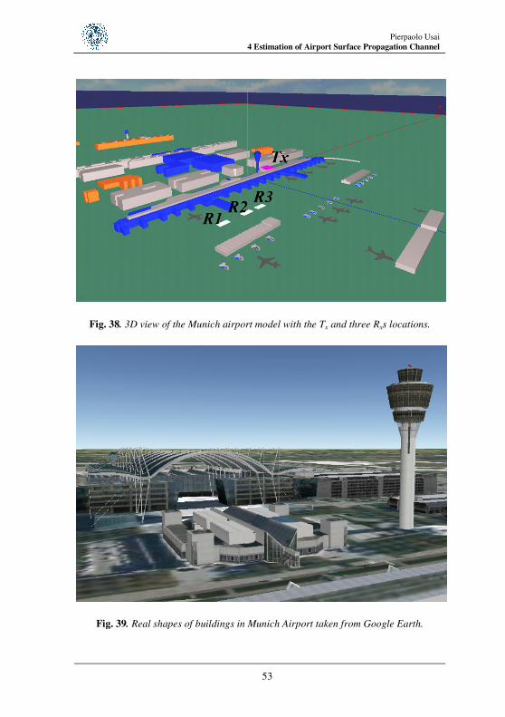
Pierpaolo Usai 4 Estimation of Airport Surface Propagation Channel
53
Fig. 38. 3D view of the Munich airport model with the Tx and three Rxs locations.
Fig. 39. Real shapes of buildings in Munich Airport taken from Google Earth.
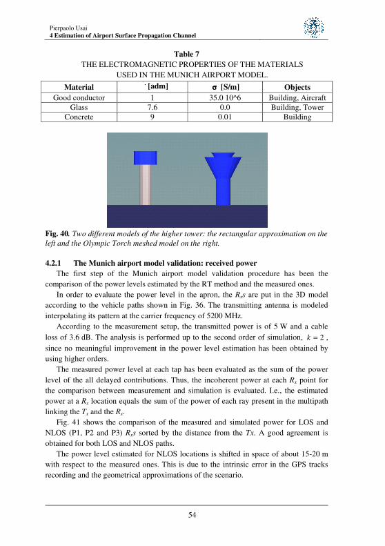
Pierpaolo Usai
4 Estimation of Airport Surface Propagation Channel
54
Table 7
THE ELECTROMAGNETIC PROPERTIES OF THE MATERIALS
USED IN THE MUNICH AIRPORT MODEL.
Material rrrrεεεε [adm] σσσσ [S/m] Objects
Good conductor 1 35.0 10^6 Building, Aircraft
Glass 7.6 0.0 Building, Tower
Concrete 9 0.01 Building
Fig. 40. Two different models of the higher tower: the rectangular approximation on the
left and the Olympic Torch meshed model on the right.
4.2.1 The Munich airport model validation: received power
The first step of the Munich airport model validation procedure has been the
comparison of the power levels estimated by the RT method and the measured ones.
In order to evaluate the power level in the apron, the Rxs are put in the 3D model
according to the vehicle paths shown in Fig. 36. The transmitting antenna is modeled
interpolating its pattern at the carrier frequency of 5200 MHz.
According to the measurement setup, the transmitted power is of 5 W and a cable
loss of 3.6 dB. The analysis is performed up to the second order of simulation, 2k = ,
since no meaningful improvement in the power level estimation has been obtained by
using higher orders.
The measured power level at each tap has been evaluated as the sum of the power
level of the all delayed contributions. Thus, the incoherent power at each Rx point for
the comparison between measurement and simulation is evaluated. I.e., the estimated
power at a Rx location equals the sum of the power of each ray present in the multipath
linking the Tx and the Rx.
Fig. 41 shows the comparison of the measured and simulated power for LOS and
NLOS (P1, P2 and P3) Rxs sorted by the distance from the Tx. A good agreement is
obtained for both LOS and NLOS paths.
The power level estimated for NLOS locations is shifted in space of about 15-20 m
with respect to the measured ones. This is due to the intrinsic error in the GPS tracks
recording and the geometrical approximations of the scenario.

Pierpaolo Usai 4 Estimation of Airport Surface Propagation Channel
55
Fig. 41. Measured and simulated power decay with the distance from the Tx.
4.3 Spreading function
In this section, the direct deterministic approach is described. The SF evaluation
starts from the direct computation of the power, delay and Doppler frequency shift per
ray.
4.3.1 The direct deterministic approach
For each receiver in the scene, the RT solver provides the number NRAY of rays
linking Rx and Tx. For each ray it also provides the power P, the length of the path L
and the direction of arrival ˆAv (unit vector). The delay τ of a ray can be expressed
starting from the path length, and the Doppler shift fD from the direction of arrival as
L
cτ = and [ ] ˆ cos( )
T
D A
f ff v v v
c cα= ⋅ = ⋅
.
where c is the speed of the light, v
the speed vector of the receiver and f the
operating frequency.
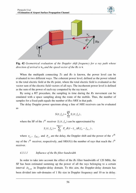
Pierpaolo Usai
4 Estimation of Airport Surface Propagation Channel
56
Fig. 42 Geometrical evaluation of the Doppler shift frequency for a ray path whose
direction of arrival is vA and the speed vector of the Rx is v.
When the multipath connecting Tx and Rx is known, the power level can be
evaluated in two different ways. The coherent power level, defined as the power related
to the total electric field at the Rx point, where the total electric field is evaluated as the
vector sum of the electric field vectors of all rays. The incoherent power level is defined
as the sum of the power of each ray computed by the ray tracer.
By using a RT procedure, the sampling in time during the Rx movement can be
emulated with a space sampling along the route of the mobile. Thus, the number of
samples for a fixed path equals the number of Rxs NRX in that path.
The delay Doppler power spectrum along a line of NRX receivers can be evaluated
as
1
( , ) ( , )NRX
D i D
i
S f S fτ τ=
=∑ ,
where the SF of the thi receiver ( , )
i DS fτ can be approximated by
( )
, , ,
1
( , ) ( ) ( )NRAY i
i D i r i r D Di r
r
S f P f fτ δ τ τ δ=
= − −∑ ,
where ,i rτ , ,Di rf and ,i rP are the delay, the Doppler shift and the power of the thr
ray of the thi receiver, respectively, and NRAY(i) the number of rays that reach the th
i
receiver.
4.3.1.1 Influence of the Rx filter bandwidth
In order to take into account the effect of the Rx filter bandwidth of 120 MHz, the
SF has been estimated summing up the power of all the rays belonging to a certain
interval ,n mD in Doppler-delay domain. To this aim, the Doppler-delay domain has
been divided into sub-domains of 1 Hz size in Doppler frequency and 10 ns in delay.

Pierpaolo Usai 4 Estimation of Airport Surface Propagation Channel
57
For each sub-domain the power is estimated as the average of the power levels of all
rays belonging to the sub-domain:
, ,1, ,
1 1( , ) ( , ) ( , )
n m n m
NRX
D i D
in m n mD D
S n m S f S fN N
τ τ=
= = ∑∫∫ ∫∫
where Nn,m is the number of rays belonging to Dn,m,
,n m n mD D Dfτ= × ,
(( 1) , )nD n nτ τ τ= − ∆ ∆ with 1,2, , MAXTn
τ=
∆…
( ( 1) , )m MAX MAXDf F m f F m f= − − ∆ − ∆
with 2
1, 2, , MAXFm
f=
∆… .
Table 8 sums up the parameters used for the discretization.
Table 8
THE PARAMETERS USED FOR THE DISCRETIZATION
OF THE DOPPLER DELAY DOMAIN.
∆∆∆∆ττττ TMAX ∆∆∆∆f FMAX
10 ns 6 µs 1 Hz 200 Hz
4.4 Munich Airport Results
In this section the simulation results of the Munich scenario analysis and their
comparison with the measurements are presented in terms of spreading function and
scatter location evaluation. The spreading function has been evaluated according to the
formulation described in the paragraph 4.3 and to the measurement settings.
4.4.1 Measured and estimated spreading function
The simulated SF has been evaluated along a path of 17.5 m which corresponds to
the distance covered by the measurement vehicle within an observation interval of 2 s
with a speed of 30 km/h. In order to select the number of Rxs per path, we compared the
results in terms of SF obtained with the choices of 18 and 171 Rxs in a path of 17.5 m,
i.e. a density of about 1 Rx/m and 10 Rx/m. Very similar results are obtained with these
two values of densities, but the higher value case showed a longer simulation time due
to the bigger number of Rxs the RT algorithm had to process.
The measured SF related to the path R1 in Fig. 38 is shown in Fig. 43 and two
simulated SFs with 18 and 171 Rxs per path in Fig. 44 and Fig. 45, respectively.
Different colours are used to identify different power levels expressed in the logarithmic
scale of dBm: in dark red the highest value and in dark blue the lowest one. The lowest
value has been fixed 50dB lower than the highest one. The same simulation settings
used for power estimation have been applied in SF evaluation. The delay offset of 4 µs
between measurements and simulations is due to a synchronization offset of 4 µs in the
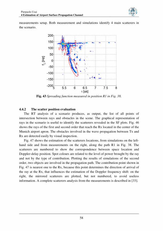
Pierpaolo Usai
4 Estimation of Airport Surface Propagation Channel
58
measurements setup. Both measurement and simulations identify 4 main scatterers in
the scenario.
Fig. 43 Spreading function measured in position R1 in Fig. 38.
4.4.2 The scatter position evaluation
The RT analysis of a scenario produces, as output, the list of all points of
intersection between rays and obstacles in the scene. The graphical representation of
rays in the scenario is useful to identify the scatterers revealed in the SF plots. Fig. 46
shows the rays of the first and second order that reach the Rx located in the center of the
Munich airport apron. The obstacles involved in the wave propagation between Tx and
Rx are detected easily by visual inspection.
Fig. 47 shows the estimation of the scatterers locations, from simulations on the left-
hand side and from measurements on the right, along the path R1 in Fig. 38. The
scatterers are numbered to show the correspondence between space location and
Doppler-delay position. Spot colours are related to the level of power brought by the ray
and not by the type of contribution. Plotting the results of simulations of the second
order, two objects are involved in the propagation path. The contribution point shown in
Fig. 47 is nearest one to the Rx, because this point determines the direction of arrival of
the ray at the Rx, that influences the estimation of the Doppler frequency shift: on the
right, the mirrored scatterers are plotted, but not numbered, to avoid useless
information. A complete scatterers analysis from the measurements is described in [33].

Pierpaolo Usai 4 Estimation of Airport Surface Propagation Channel
59
Fig. 44 Simulated spreading function in position R1 in Fig. 38 with 18 Rxs per path.
Fig. 45 Simulated spreading function in position R1 in Fig. 38 with 171 Rxs per path.
The calculation of the scatterers positions from the measured data ( ), Dfτ is based
on the hypothesis that scatterers result from single and not multiple reflections, [32].
These locations are obtained by the intersection between the line at an angle α with
respect to the speed vector and the ellipse with focuses in the Tx and Rx and
circumference dependent on τ. Because of the ambiguity in the angle of incidence
evaluation = ±arccos( / )Dc f v fα ⋅ ⋅ , with c the speed of light, there are two possible
intersection points for each scatterer. However, this drawback can be overcome by
employing a priori knowledge of the environment.

Pierpaolo Usai
4 Estimation of Airport Surface Propagation Channel
60
Fig. 46 Visualization of the rays connecting the Tx and the Rx located in the apron.
Fig. 47 Simulated scatterers positions, on the left, and measured scatterers
locations, on the right, related to the path R1 in Fig. 38.
4.4.3 Spreading function trend along the R1-R2-R3 path
In order to compare the simulation results with measurements, the changes of the SF
properties along the path R1-R2-R3 in Fig. 38 and the buildings involved in the
propagation are shown by referring to the following plots:
• the measured SF in R1, R2 and R3 (Fig. 43, Fig. 48 and Fig. 51, respectively);
• the simulated SF in R1, R2 and R3 with 18 Rxs per path (Fig. 44, Fig. 49 and
Fig. 52, respectively);
• the simulated and measured scatterers location in R1, R2 and R3 (Fig. 47, Fig.
50 and Fig. 53, respectively).
In the simulations, the LOS scatterer (1), related to the direct path coming from the
Tx, moves down on the Doppler axis as the Rx moves towards the Tx. In Fig. 47, Fig. 50
and Fig. 53, on the left side, the red spot near the scatterer (1) represents the direct path
contribution and the blue ones diffractions from the roof of the Terminal 1 building.
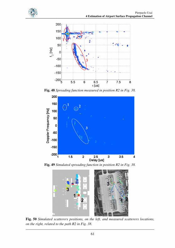
Pierpaolo Usai 4 Estimation of Airport Surface Propagation Channel
61
Fig. 48 Spreading function measured in position R2 in Fig. 38.
Fig. 49 Simulated spreading function in position R2 in Fig. 38.
Fig. 50 Simulated scatterers positions, on the left, and measured scatterers locations,
on the right, related to the path R2 in Fig. 38.
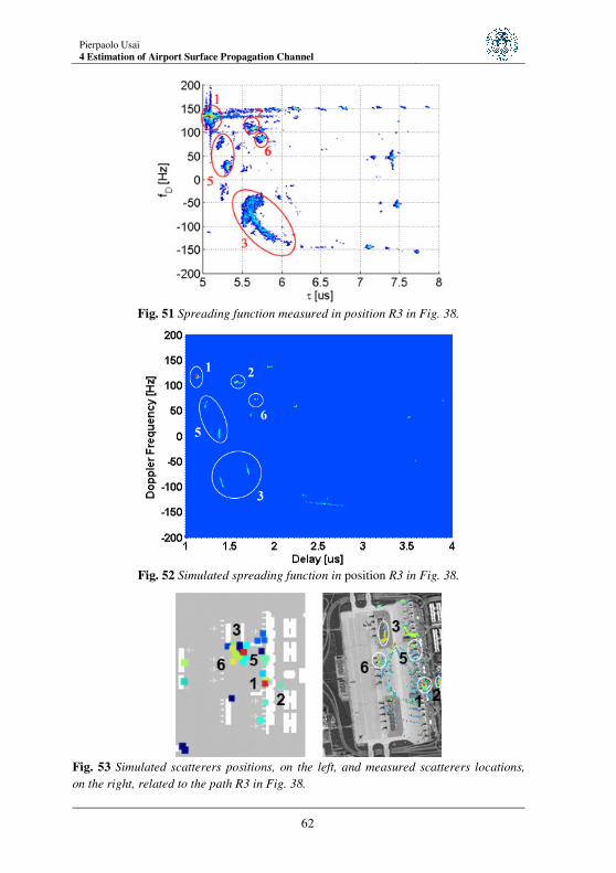
Pierpaolo Usai
4 Estimation of Airport Surface Propagation Channel
62
Fig. 51 Spreading function measured in position R3 in Fig. 38.
Fig. 52 Simulated spreading function in position R3 in Fig. 38.
Fig. 53 Simulated scatterers positions, on the left, and measured scatterers locations,
on the right, related to the path R3 in Fig. 38.

Pierpaolo Usai 4 Estimation of Airport Surface Propagation Channel
63
The red spot near the Rx position is a reflection occurring on the ground and it is
present in the three Rx positions.
The scatterer (2) is always revealed from simulations in the three locations R1-R2-
R3. The simulation analysis confirms that this scatterer is a contribution from the tower
as well as the measurements analysis have announced in advance. From the RT output
visualization it can be noticed that all contributions coming from the top of the tower
are diffractions.
The clustered scatterers (3) and (4) also move to lower Doppler frequencies and
toward higher delays. The most significant contributions coming from the scatterers (3)
and (4) are some reflections occurring on the front of the building and many diffractions
from the roof. In Fig. 47, on the left side, the red spot represents the reflection
contribution in the scatterers cluster (3), in yellow and blue the diffractions. In Fig. 50
and Fig. 53 the cluster (3) is characterized by only diffractions. The scatterers (5) and
(6) appear only in the position R3. A similar behavior was observed in the SF evaluated
from the measurements. In Fig. 52 the presence of (5)-(6) is due to diffraction
contributions only.
4.5 Simulation time comparison
The evaluation of the SF has been conducted in the locations R1, R2 e R3 of Fig. 38
by using the canonical procedure described in 3.4 paragraph. To apply the Fourier
transform based procedure the number of time samples, i.e. the number of Rxs, has been
fixed as in the measurement settings to 1024. The resulting SF in positions R1, R2 and
R3 are shown in Fig. 54, Fig. 55 and Fig. 56.
Fig. 54 Simulated spreading function in position R1 in Fig. 38 by the canonical
approach.
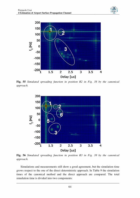
Pierpaolo Usai
4 Estimation of Airport Surface Propagation Channel
64
Fig. 55 Simulated spreading function in position R2 in Fig. 38 by the canonical
approach.
Fig. 56 Simulated spreading function in position R3 in Fig. 38 by the canonical
approach.
Simulations and measurements still show a good agreement, but the simulation time
grows respect to the one of the direct deterministic approach. In Table 9 the simulation
times of the canonical method and the direct approach are compared. The total
simulation time is divided into two components:

Pierpaolo Usai 4 Estimation of Airport Surface Propagation Channel
65
1. the ray tracing time, that refers to the time the solver needs to compute the
electric field for all the Rxs in the considered path;
2. the SF simulation time, that refers to the time the canonical and the direct
procedures need to compute the SF.
All the simulation has been performed by an Intel Core CPU i5, with 8 GB of RAM.
For the direct approach the two choices of number of Rxs, 18 and 171, are considered.
The simulation time of the canonical approach increases for two reasons:
1. a greater number of Rxs has to be considered to satisfy the sampling
theorem to solve the Fourier transform and this causes a growth of the ray
tracing time;
2. the two Fourier transforms evaluation to compute the SF is a time
consuming procedure respect to the geometrical evaluation of the Doppler
shift. To reduce this part of the simulation time the Fast Fourier Transform
algorithms could be implemented.
Table 9
Direct deterministic
Approach
Canonical
Approach
Number of Rxs 18 171 1024
Ray tracing time - A <0.1s 0.3s 1.4s
SF simulation time - B <0.1s 1.3s 331.6s
Total simulation time
(A+B)
<0.2s 1.6s 333.0s

Pierpaolo Usai
4 Estimation of Airport Surface Propagation Channel
66

Pierpaolo Usai 5 Scattering Matrix
67
5 Scattering Matrix
Description of a Physical Optics based scattering
propagation solver and its employment in the radar
cross section estimation of static or rotating objects
with metallic or dielectric surface material properties.
The Radar Cross Section - RCS evaluation of metal and dielectric objects starts from
the estimation of the objects scattered field whose information is summed up in the so-
called scattering matrix. The scattering matrix prediction by the asymptotic methods
allows to overcome the limitations the full-wave techniques present at high frequencies.
The approximations introduced by the assumption of far-field sources and observers at
high frequencies allow to unburden the calculation procedures obtaining good
estimations of the scattered field. The Physical Optics - PO theory is the most diffuse
solution solving these kind of problems, often together with a ray bouncing analysis to
predict the illuminated facets of the object, [34][35] . PO approximates the currents
flowing on an illuminated meshed object to that there would be on an infinite plane
layered on each of its lit polygonal facet. By the radiation integral evaluation of these
currents the scattered electric field is estimated with a reduction in simulation time
respect to a full-wave analysis. The PO formulation estimates the reflection of the wave
front impinging on an object. If the contribution of diffraction from edges wants to be
considered in the field prediction, the Physical Theory of Diffraction have to be
invoked, [35].
There are three main hypotheses a scenario must satisfy to be analyzed by the PO
method, [36]:1) the wavelength is short with the object dimensions and field amplitudes
rapidly decay on surfaces which are not illuminated by the incident field; 2) the main
radii of curvature of the directly lighted object surface significantly exceed the
wavelength; 3) the observation distance is very large with respect to the size of the
object.

Pierpaolo Usai
5 Scattering Matrix
68
To solve the scattering matrix prediction of metallic and dielectric objects a PO
based solver has been implemented. The object is assumed formed by a triangular mesh
so that only the illuminated triangles radiate the field towards the observer. Having
fixed the triangular shape of the mesh, the radiation integral on the illuminated part of
the object is decomposed in the sum of the fields radiated by each lit triangular facet. A
close solution of the radiation integral has been computed on the triangular space
domain in a local reference system. The scattered field predicted by the solver has been
employed to evaluate the monostatic and bistatic scattering matrix of an object, and so,
its radar cross section profile. The solver results have been used also to estimate the
radar cross section spectrum of object rotating at constant angular velocity around a
fixed axis.
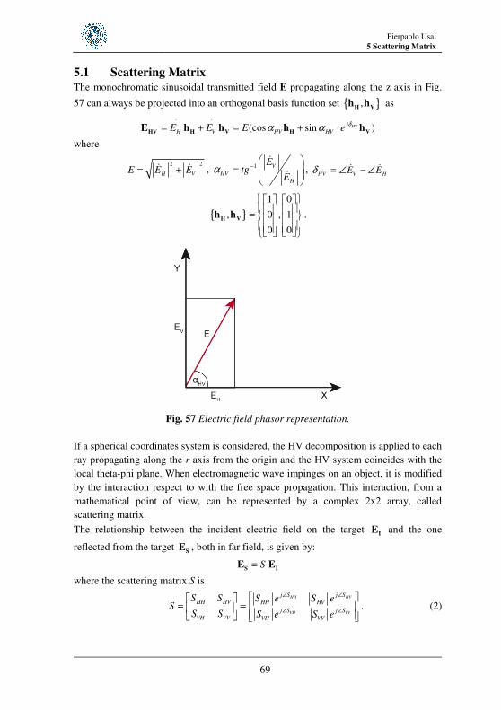
Pierpaolo Usai 5 Scattering Matrix
69
5.1 Scattering Matrix
The monochromatic sinusoidal transmitted field E propagating along the z axis in Fig.
57 can always be projected into an orthogonal basis function set ,H V
h h as
(cos sin )HVj
H V HV HVE E E e
δα α⋅ ⋅
= + = + ⋅HV H V H V
E h h h h
where
2 2
H VE E E= +ɺ ɺ , 1 V
HV
H
Etg
Eα −
=
ɺ
ɺ , HV V H
E Eδ = ∠ − ∠ɺ ɺ
1 0
, 0 , 1
0 0
=
H Vh h .
Fig. 57 Electric field phasor representation.
If a spherical coordinates system is considered, the HV decomposition is applied to each
ray propagating along the r axis from the origin and the HV system coincides with the
local theta-phi plane. When electromagnetic wave impinges on an object, it is modified
by the interaction respect to with the free space propagation. This interaction, from a
mathematical point of view, can be represented by a complex 2x2 array, called
scattering matrix.
The relationship between the incident electric field on the target I
E and the one
reflected from the target S
E , both in far field, is given by:
S=S I
E E
where the scattering matrix S is
HVHH
VH VV
j Sj S
HH HV HH HV
j S j S
VH VV VH VV
S S S e S eS
S S S e S e
∠∠
∠ ∠
= =
. (2)

Pierpaolo Usai
5 Scattering Matrix
70
This matrix depends on frequency, the physical and geometrical characteristics of the
target and its orientation with respect to the observer antenna.
The scattering matrix coefficients are related to the radar cross section parameter by the
following relations 224HH HHR Sσ π=
224HV HVR Sσ π=
224VH VHR Sσ π=
224VV VVR Sσ π=
where R is the distance between the receiver and the target. In the previous relationships
the subscript on the left is related to the polarization in reception, while the right one to
the polarization in transmission.
Fig. 58 Incident and scattered electric field representation.
To calculate the matrix coefficients, the scattered electric field has to be estimated. So
the scattering matrix estimation depends on the possibility of computing the scattered
field. To this aim, in the following the PO method and a PO based electromagnetic
solver will be described.
5.2 PO based numerical solver
The Physical Optics high frequencies method allows to approximate the scattered
field from an illuminated object placed in the far field of a source with the one radiated
by the surface currents inducted by the source on the object.
To model a realistic object surface, it is necessary to create a discretization that
faithfully preserves its geometric shape, and at the same time allows a tractable and
numerically efficient computation of the radiation integral. The most popular method of
discretization is a surface tessellation into a wavelength-dependant number of plane
polygons (facets).
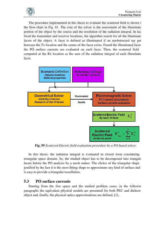
The procedure implemented in this thesis to evaluate t
the flow-chart in Fig. 61. The core of the solver is the assessment
portion of the object by the source and the resolution of the radiation integral
fixed the transmitter and receiver locations, the algorithm
facets of the object. A facet is defined as illuminated if
between the Tx location and the center of the facet exists.
the PO surface currents are evaluated on each facet. Then, the scattered field is
computed at the Rx location as the sum of the radiation integral of each illuminated
facet.
Fig. 59 Scattered Electric field evaluation procedure by a PO based
In this thesis, the radiation integral is evaluated in
triangular space domain. So, the studied object has to be decomposed into triangular
facets before the PO analysis by a mesh maker. The choice of the triangular shap
justified by the fact it is the most fitting shape to approximate any kind of surface
is easy to provide a triangular tessellation.
5.3 PO surface currents
Starting from the free space and the studied problem
paragraphs the equivalent physical models are presented for both
object and, finally, the physical optics approximations are defined
Pierpaolo Usai
5 Scattering Matrix
The procedure implemented in this thesis to evaluate the scattered field is shown in
is the assessment of the illuminated
of the radiation integral. In fact,
algorithm search for all the illuminated
defined as illuminated if an unobstructed ray path
between the Tx location and the center of the facet exists. Found the illuminated facets
ce currents are evaluated on each facet. Then, the scattered field is
computed at the Rx location as the sum of the radiation integral of each illuminated
Electric field evaluation procedure by a PO based solver.
in closed form considering a
object has to be decomposed into triangular
facets before the PO analysis by a mesh maker. The choice of the triangular shape is
justified by the fact it is the most fitting shape to approximate any kind of surface and it
the free space and the studied problem cases, in the following
presented for both PEC and dielectric
s are defined, [1].
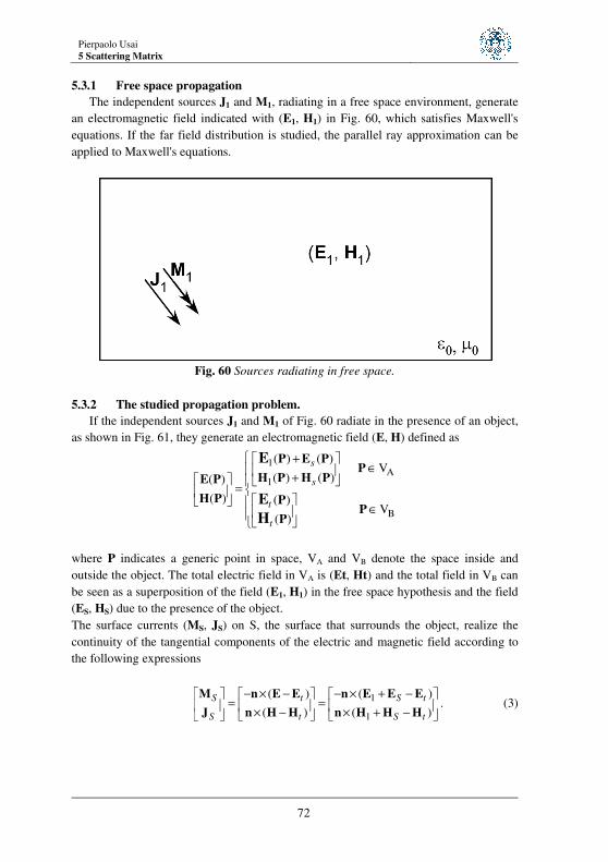
Pierpaolo Usai
5 Scattering Matrix
72
5.3.1 Free space propagation
The independent sources J1 and M1, radiating in a free space environment, generate
an electromagnetic field indicated with (E1, H1) in Fig. 60, which satisfies Maxwell's
equations. If the far field distribution is studied, the parallel ray approximation can be
applied to Maxwell's equations.
Fig. 60 Sources radiating in free space.
5.3.2 The studied propagation problem.
If the independent sources J1 and M1 of Fig. 60 radiate in the presence of an object,
as shown in Fig. 61, they generate an electromagnetic field (E, H) defined as
1A
1
B
( ) ( ) V
( ) ( )( )
( ) ( ) V
( )
s
s
t
t
+ ∈
+ =
∈
P E PP
H P H PE P
H P PP
P
E
E
H
where P indicates a generic point in space, VA and VB denote the space inside and
outside the object. The total electric field in VA is (Et, Ht) and the total field in VB can
be seen as a superposition of the field (E1, H1) in the free space hypothesis and the field
(ES, HS) due to the presence of the object.
The surface currents (MS, JS) on S, the surface that surrounds the object, realize the
continuity of the tangential components of the electric and magnetic field according to
the following expressions
1
1
( ) ( )
( ) ( )
S t S t
S t S t
− × − − × + − = = × − × + −
M n E E n E E E
J n H H n H H H. (3)
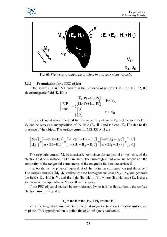
Pierpaolo Usai 5 Scattering Matrix
73
Fig. 61 The wave propagation problem in presence of an obstacle.
5.3.3 Formulation for a PEC object
If the sources J1 and M1 radiate in the presence of an object in PEC, Fig. 62, the
electromagnetic field (E, H) is
1A
1
B
( ) ( ) V
( ) ( )( )
( ) 0 V
0
s
s
+ ∈
+ =
∈
P E PP
H P H PE P
H PP
E
In case of metal object the total field is zero everywhere in VA and the total field in
VB can be seen as a superposition of the field (E1, H1) and the one (ES, HS) due to the
presence of the object. The surface currents (MS, JS) on S are
1 1
1 1
( ) ( ) ( ) 0
( ) ( ) ( ) 0
S t S t S
S t S t S
− × − − × + − − × + = = = = = × − × + − × + ≠
M n E E n E E E n E E
J n H H n H H H n H H.
The magnetic current MS is identically zero since the tangential components of the
electric field on a surface in PEC are zero. The current JS is not zero and depends on the
continuity of the tangential components of the magnetic field on the surface S.
Fig. 63 shows the physical equivalent of the radiation configuration just described.
The surface currents (MS, JS) radiate into the homogeneous space VA + VB and generate
the field (-E1, -H1) in VA and the field (ES, HS) in VB, where (E1, H1) and (ES, HS) are
solutions of the equations of Maxwell in free space.
If the PEC object shape can be approximated by an infinite flat surface, , the surface
electric current is equal to
1 1( ) 2S S= × = × + = ×J n H n H H n H
since the tangential components of the total magnetic field on the metal surface are
in phase. This approximation is called the physical optics equivalent.
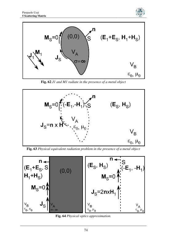
Pierpaolo Usai
5 Scattering Matrix
74
Fig. 62 J1 and M1 radiate in the presence of a metal object
Fig. 63 Physical equivalent radiation problem in the presence of a metal object
Fig. 64 Physical optics approximation.

Pierpaolo Usai 5 Scattering Matrix
75
5.3.4 Formulation for a dielectric object
The simplification of the studied propagation problem in case of a PEC object
cannot be repeated in the case of a dielectric object. In fact, the surface currents in (3)
must radiate in the presence of the object and no approximation may be applied starting
from the material properties, but from the objet shape. If the object can be approximated
by an infinite plane, the currents on the dielectric surface may be described as
1
1
( ) ( )
( ) ( )
S S R inc
S S R inc
− × + − × +− × = = = × + × +×
M n E E n E En E
J n H H n H Hn H
where ER is the reflected electric calculated as described in paragraph 1.4. This
approximation is called the physical optics equivalent for dielectric surface.
5.4 PO radiation integral
In this section the radiation integral formulation according to the physical optics
equivalent currents approximation is presented both for PEC and dielectric solutions.
5.4.1 PEC object
The scattered electric field derived by the PO method is based on solving the
radiation integral of the space depending surface currents. In the case of metallic object
the electric field in the far field region is computed as follows
jω≅ −S
E A , j re βµ −=A N
cos cosˆ( ) 2 ( )
i
j r j r
S i
iS S
e dS n e dSβ ψ β ψ′ ′′ ′= = ×∑∫∫ ∫∫ 1N J P H P
where the object surface S is decomposed in Nf planar polygons and 1
Nf
iiS S
==∪ .
Considering the space domain Si in Fig. 65, where a triangular shape of the mesh is
fixed, the radiation integral may be evaluated as the product of the current in the origin
of the local coordinates system X’Y’Z’ and a 2D integral that can be solved in closed
form, [37]. ˆ ˆcos cos
ˆ '( sin sin )'( sin cos )cos
ˆ ˆ2 ( ) 2 ( )
ˆ2 ( ) ( ) .
i i
yx
i i
j r j r j r j r
i i
S S
j y vj x vj r j r
S S
n e e dS z e e dS
z e e dS e e dx dy
β β ψ β β ψ
β θ ϕβ θ ϕβ β ψ ′′
′ ′− • − •
− −′ − −− •
′ ′ ′× = × =
′ ′ ′ ′= × =
∫∫ ∫∫
∫∫ ∫∫
1 i 1 i
1 i s i
H P1 H P1
H P1 J P1
(4)
Fig. 65 Triangular space domain of the radiation integral.

Pierpaolo Usai
5 Scattering Matrix
76
5.4.2 Dielectric object
If the object is made of a dielectric material, the scattered electromagnetic field in
the far field region may be evaluated as
jω≅ −S
E A , j re
βµ −=A N ,
( )cos cos( ) ( ) ( )
i
j r j r
S R inc i
iS S
e dS e dSβ ψ β ψ′ ′′ ′= = × +∑∫∫ ∫∫ i iN J P n H P H P and
jω≅ −S
H F , j re
βµ −=F L ,
( )cos cos( ) ( ) ( )
i
j r j r
S R inc i
iS S
e dS e dSβ ψ β ψ′ ′′ ′= = − × +∑∫∫ ∫∫ i iL M P n E P E P
where 1
Nf
iiS S
==∪ is a mesh partition of the object. As the PEC object formulation, the
currents integration over the whole surface of the object is split in the sum of the
integrals evaluated over each triangular facet
( )
( )
( )
( )
cos
ˆ cos
ˆ cos
'( sin sin )'( sin cos )
( ) ( )
( ) ( )
( ) ( )
( ) ( )
i
i
i
yx
i
j r
R inc i
S
j r j r
R inc i
S
j r j r
R inc i
S
j y vj x v
R inc
S
e dS
e e dS
e e dS
e e dx dy
β ψ
β β ψ
β β ψ
β θ ϕβ θ ϕ ′′
′
′− •
′− •
− −− −
′× + =
′= × + =
′= × + =
′ ′= × +
∫∫
∫∫
∫∫
∫∫
i i
i i
i i
i i
n H P H P
n H P1 H P1
n H P1 H P1
n H P1 H P1
(5)
and
( )
( )
( )
( )
cos
ˆ cos
ˆ cos
'( sin sin )'( sin cos )
( ) ( )
( ) ( )
( ) ( )
( ) ( )
i
i
i
yx
i
j r
R inc i
S
j r j r
R inc i
S
j r j r
R inc i
S
j y vj x v
R inc
S
e dS
e e dS
e e dS
e e dx dy
β ψ
β β ψ
β β ψ
β θ ϕβ θ ϕ ′′
′
′− •
′− •
− −− −
′− × + =
′= − × + =
′= − × + =
′ ′= − × +
∫∫
∫∫
∫∫
∫
i i
i i
i i
i i
n E P E P
n E P1 E P1
n E P1 E P1
n E P1 E P1
.∫
(6)
5.4.3 Solution of the radiation integral on a triangular domain
Let’s consider a function s(x,y) defined on a triangular domain Si as
1 ( , )
0
i
i
(x, y) Ss x y
(x, y) S
∈=
∉.
Its Fourier transform is known in closed form for any polygon shape domain Si, [37],
and it may be written as
( , ) ( , )
i
jux vy jux vy
S
S u v s x y e dxdy e dxdy
∞ ∞− + − +
−∞ −∞
= =∫ ∫ ∫∫ . (7)
The integrals in (4), (5) and (6) can be easily reduced into the (7) formulation by the
following definitions

Pierpaolo Usai 5 Scattering Matrix
77
'
'
( sin cos ) (sin cos sin cos )
( sin sin ) (sin sin sin sin )
x sc sc in in sc sc
y sc sc in in sc sc
u v
v v
β θ ϕ β θ ϕ θ ϕ
β θ ϕ β θ ϕ θ ϕ
= − = −
= − = −.
The analytical solution of (7) is expressed according to the zero values assumed by the u
and v frequencies. Table 10 shows the four ranges of the u-v variable frequencies
respect to which the integral in (7) is computed.
Table 10
S(u,v) INTEGRAL vs FREQUENCIES RANGES
S(u,v) u = 0 u ≠ 0
v = 0 Surface of Si Su
v ≠ 0 Sv Suv
If u=0 and v=0, then
( )(0,0)
i i
j ux vy
i
S S
S e dxdy dxdy S− +
= = =∫∫ ∫∫ .
If u≠0 and v=0, then
( ,0)
i
jux
u
S
S u S e dxdy−= = ∫∫ .
If u=0 and v≠0, then
(0, )
i
jvy
v
S
S v S e dxdy−= = ∫∫ .
If u≠0 and v≠0, then
( )( , )
i
j ux vy
S
S u v e dxdy− +
= ∫∫ .
The exact solution for each of the four integration cases is reported with details in
Appendix A.
5.5 Estimation of the RCS parameter
From the scattering matrix of equation (2), it is obvious that in monostatic
scattering, i.e., the incident and scattering directions coincide, VV HH
S S= and
0HV VH
S S= = . In this case the co-polarized fields are identical, and the cross-polarized
fields are zero. In fact, the PO approximation does not involve non-uniform fringe
currents, multiple reflections, or depolarizing scatterers, [38][39].
In this section the estimated RCS of a dodecahedron, whose side length is 0.42m, by
the PO based solver is compared with the solution obtained by using the commercial
software FEKO implementing a PO based tool. The monostatic and bistatic RCS are
shown both for a PEC and dielectric dodecahedron.
5.5.1 Case of study: PEC dodecahedron
The PEC dodecahedron RCS is evaluated at the single frequency of 3 GHz in linear
polarization. The monostatic RCS is evaluated around the object in the plane 90θ = °
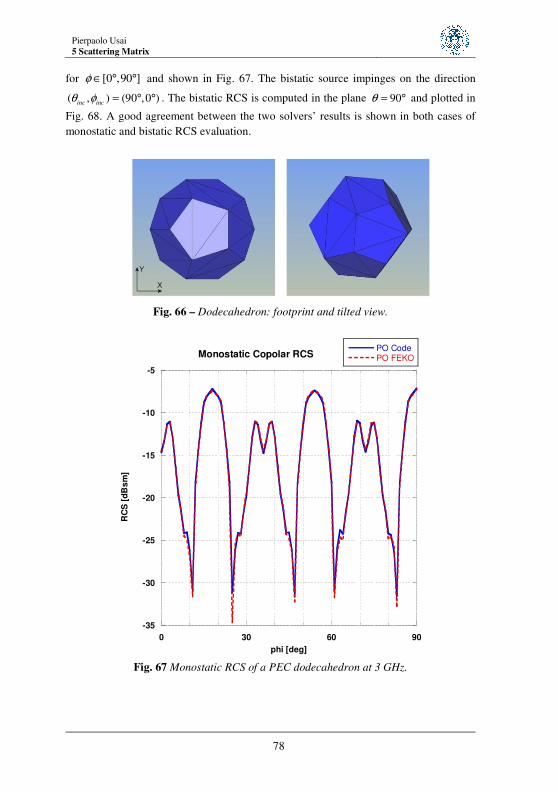
Pierpaolo Usai
5 Scattering Matrix
78
for [0 ,90 ]φ ∈ ° ° and shown in Fig. 67. The bistatic source impinges on the direction
( , ) (90 ,0 )inc inc
θ φ = ° ° . The bistatic RCS is computed in the plane 90θ = ° and plotted in
Fig. 68. A good agreement between the two solvers’ results is shown in both cases of
monostatic and bistatic RCS evaluation.
Fig. 66 – Dodecahedron: footprint and tilted view.
-35
-30
-25
-20
-15
-10
-5
0 30 60 90
Monostatic Copolar RCSPO CodePO FEKO
RC
S [
dB
sm
]
phi [deg]
Fig. 67 Monostatic RCS of a PEC dodecahedron at 3 GHz.

Pierpaolo Usai 5 Scattering Matrix
79
-60
-40
-20
0
20
40
0 60 120 180 240 300 360
Bistatic Copolar RCS Theta=90° Phi=0°
PO CodePO FEKO
RC
S [
dB
sm
]
phi [deg]
Fig. 68 Bistatic RCS of a PEC dodecahedron at 3 GHz.
5.5.2 Case of study: dielectric dodecahedron
The dielectric dodecahedron RCS is evaluated at the single frequency of 3 GHz in
linear polarization too. The electromagnetic properties of the dielectric object are a
dielectric permittivity of 9.0 and an electric conductivity of 0.01 S/m. The monostatic
RCS is evaluated around the object in the plane 90θ = ° for [0 ,90 ]φ ∈ ° ° and shown in
Fig. 69. The bistatic incident direction is ( , ) (90 ,0 )inc inc
θ φ = ° ° . The bistatic RCS is
computed in the plane 90θ = ° and plotted in Fig. 70. A good agreement between the
two solvers’ results is shown in both cases of monostatic and bistatic RCS evaluation
for the dielectric object too.
5.5.3 Simulation time comparison
Table 11 shows the comparison of the simulation time of the PO code and the FEKO
one, when the analysis in paragraph 5.5.2 is conducted. The PO code simulation results
faster than the FEKO one, because its object's mesh has made by using facets whose
sizes are as bigger as possible. On the contrary FEKO implementation meshes the
object by facets whose sizes are smaller than the wave-length. All the simulation has
been performed by an Intel Core CPU i5, with 8 GB of RAM.

Pierpaolo Usai
5 Scattering Matrix
80
-50
-45
-40
-35
-30
-25
-20
-15
-10
0 15 30 45 60 75 90
Monostatic CoPolar RCS epsr=9 sigma=0.01S/m
PO CodePO FEKO
RC
S [
dB
sm
]
phi [deg]
Fig. 69 Monostatic RCS of a dielectric dodecahedron at 3 GHz.
-80
-60
-40
-20
0
20
40
0 60 120 180 240 300 360
Bistatic CoPolar RCS epsr=9 sigma=0.01S/m
PO Code
PO FEKO
RC
S [
dB
sm
]
phi [deg]
Fig. 70 Bistatic RCS of a dielectric dodecahedron at 3 GHz.

Pierpaolo Usai 5 Scattering Matrix
81
Table 11
SIMULATION TIMES COMPARISON
Simulation Time Num. of facets Num. PO basis function
PO Code 1.1s 36 36
PO FEKO 151.4s 36 209490
5.6 RCS Spectrum of rotating objects
To estimate the Doppler frequency shift RCS components a rotating body provides
when it is illuminated by an electromagnetic source at high frequency, the first step is to
evaluate the scattered electric field of the rotating object during a period of its
revolution. If the revolution period is sampled in N intervals with a sample step of t∆ ,
the PO approach may be used to estimate the Scattering Matrix per time sample fixed
the incident and observation directions. The RCS distribution versus the Doppler
frequency shift is computed by the Fourier transform of the complex diffusion
coefficient as
( , , , , ) ( ( , , , , ))in in sc sc D in in sc sc
S f FT S tθ φ θ φ θ φ θ φ= .
The evaluation of the complex diffusion coefficient on a period is realized by fixing
the source and observation directions and rotating the object around the rotation axis
according to the law of motion. If the vector rotation frequency is ω , each facet vertex
moves according to the law ( ) (0)t t= + ×P P R ω , where P(0) is the initial location and
R the vector distance of the vertex by the rotation axis.
5.6.1 Case of study: 2-blades
Blades have a profile depending on the application they are used. A typical
helicopter blade with its profile is shown in Fig. 71. A couple of this type of blade with
a counter-clockwise angular velocity of 1320°/s in the xy-plane, Fig. 72, has been
characterized in terms of RCS spectrum. The monostatic RCS spectrum of the rotating
blades at the frequency of 5GHz is shown in Fig. 73, when the incident direction is
( , ) (68.2 ,90 )inc inc
θ φ = ° ° with a linear polarization (vertical).
Fig. 71 A typical helicopter blade’s profile.

Pierpaolo Usai
5 Scattering Matrix
82
Fig. 72 2blades rotating around the z-axis.
-70
-60
-50
-40
-30
-20
-10
0
10
-10 -5 0 5 10
RCS Spectrum
RC
S [
dB
sm
]
Doppler Freqency Shift [KHz]
Fig. 73 RCS spectrum of the 2-blades in Fig. 72 at 5GHz.
The negative doppler shifts dominate because of the blade profile and the counter
clockwise angular velocity considered in the simulation. The profile influence on the
RCS spectrum evaluation could be used to characterize blade's profiles by predicting the
RCS spreading in the Doppler frequency shift domain.

Pierpaolo Usai Appendix A
83
Appendix A – Radiation
Integral on a triangular space
domain
The local Cartesian system of coordinates with the origin in the P1 vertex and the
P2 point lying in the positive x semi axis may be considered without loss of generality,
Fig. 74.
Fig. 74 Triangular domain in the local coordinates system with the origin in P1 vertex
and a second vertex (P2) lying on the positive x axis.
Let’s consider a function s(x,y) defined on the triangular domain Si as
1 ( , )
0
i
i
(x, y) Ss x y
(x, y) S
∈=
∉
and its Fourier transform
( ) ( )
( ) ( ) ( ) ( )3 3 3 3 3 32 2
1 1 3 1 30 0 0
( , ) ( , )
i
j ux vy j ux vy
S
x y y x y yx x
j ux vy j ux vy j ux vy j ux vy
x y x y x
S u v s x y e dxdy e dxdy
e dxdy e dxdy e dxdy e dxdy
∞ ∞− + − +
−∞ −∞
− + − + − + − +
= = =
= + = +
∫ ∫ ∫∫
∫ ∫ ∫ ∫ ∫ ∫ ∫ ∫

Pierpaolo Usai
Appendix A
84
where 1 1 11 [ , , ]P x y z= ,
2 2 22 [ , , ]P x y z= and 3 3 33 [ , , ]P x y z= are the vertices of Si in
Fig. 74.
The S function can be evaluated splitting the integral calculation into 4 main cases:
1. CASE u=0, v=0
( ) 2 3(0, 0)2
i i
j ux vy
i
S S
x yS e dxdy dxdy S
− + ⋅= = = =∫∫ ∫∫ .
2. CASE u≠0, v=0
3 3 32
30 0 0
( ,0) ( ) 1( ) 2( )
i
x y yx
jux jux jux
u
S x
S u S u e dxdy e dxdy e dxdy S u S u− − −= = == + = +∫∫ ∫ ∫ ∫ ∫
3-3
3 32
3
3
1(1- (1 ) ) if x 0
1( )if x =0
0
juxyjux e
x uS u
+ ≠
=
( )( )323
2 32
2 3
11 ( ) if
2( )if
0
juxjux
3 2
3 2
yju x x e e x x
x x uS ux x
−−+ − − ≠
−= =
.
3. CASE u=0, v≠0
3 3 32
30 0 0
(0, ) ( ) 3( ) 4( )
i
x y yx
jvy jvy jvy
v
S x
S v S v e dxdy e dxdy e dxdy S v S v− − −= = = + = +∫∫ ∫ ∫ ∫ ∫
3-3
3 32
3
3
1(1 )if x 0
3if x =0
0
jvyxjvy e
y vS
− − ≠
=
( ) ( )2
2 3
3 3
2
2 32 3
2
3 3
11 if
4if
0
x xjv
jvy y
3 2
3 2
x xx xe e jv x x
S y yvx x
−−
−
−− − − ≠ = =
.
4.CASE u≠0, v≠0
( ) ( ) ( )3 3 32
30 0 0
( , ) 5 6
i
x y yx
j ux vy j ux vy j ux vy
S x
S u v e dxdy e dxdy e dxdy S S− + − + − += = + = +∫∫ ∫ ∫ ∫ ∫
3
3 3 3
3
3
3
3 ( )
3
3
3
1 1( ) if 0
if x 05 1 1
if 0
if x =0 0
jux
j ux vy jux
yex a u v
jv ju x
S ye ea u v
va uv x
−
− + −
−− − = + =
≠ = − − − = + ≠

Pierpaolo Usai Appendix A
85
3 32
3
3 3 3 32 2
3
2 3
2 3
3 2 ( )
3
2 3
3 2
( ) if 0
if x x6
if 0
if x =x 0
jvy juxjuxjux
jvy j a u x jax juxjax jux
ye e ee x x a u v
jv ju x x
S ye e e e e ea u v
jv ja ju x x
− −−−
− − − −− −
−− + = − =
− ≠
= − −− = − ≠ − − −

Pierpaolo Usai
Appendix A
86
Pierpaolo Usai
Conclusions
87
Conclusions
In this thesis, the asymptotic methods has been applied to solve a number of
electromagnetic problems involved in modern high frequency wireless systems.
The main steps of a ray tracing based solver for wave propagation prediction in
complex scenario has been presented. In particular, the evaluation of the electric field
has been defined as the sum of the electric field related to each ray of the multipath
computed by the ray tracing algorithm. Four types of contributions have been presented
direct path, reflection, diffraction and transmission. A detailed description of the electric
field evaluation for each type of contribute has been given.
An arbitrary and flexible shape selection of the investigated area for a ray tracing
analysis has been proposed. The method is particularly suitable for evaluating
propagation in urban scenarios where not all the objects are involved in the ray
propagation between the transmitter and the receiver. There is no restriction to
canonical shapes such as circles or ellipses for the selection of the area under test, since
the partitioning into voxel provides the user to define irregular polygons thus avoiding
to include unnecessary elements. The accuracy of the method and its performances in
terms of ray tracing time have been proved by using comparison between simulations
and measurements. It has also been shown that the algorithm allows to consider high
simulation orders in a considerable shorter ray tracing time with respect to a full ray
tracing analysis.
The frequency response of a wireless channel has been defined when the radio link
can be considered a linear and time invariant system. The channel has been defined as
effective or pure, respectively, if the influence of the antennas are taken into account or
not in the system frequency response evaluation. To this aim, the characterization of the
channel needs to model the antennas in terms of transfer function, i.e., to model the
antennas frequency-dependant behavior. By means of the Fourier transform of the
frequency response, the system impulse response may be evaluated. The power delay
profile and time delay characteristics, as the mean time of arrival and the root mean
squared delay spread, have been directly derived by the impulse response. When the Rx
moves in the scene, the spreading function sums up the channel behavior in terms of
power distribution in the Doppler shift-delay domain. The spreading function has been
defined as the Fourier transform of the impulse response respect to time, in the

Pierapolo Usai
Conclusions
88
hypothesis of linearity and time invariance of the wireless system for each time sample
of the observation time. A simple scenario has been used to show how the rays
contributions combine to characterize the channel frequency response in a baseband
analysis. The simulation of the propagation inside an empty room has been validated by
the comparison of the measured average power delay profile with the simulated one, in
the case of a passband transmitted signal. Finally, the in-phase and in-quadrature
components of the impulse response have been estimated.
The electromagnetic model of an airport environment has been built up to
characterize the wireless communication channel between a fixed transmitter and a
moving receiver in the apron. The Munich scenario has been validated by comparing
measured and simulated power values. The spreading function has been evaluated by
the canonical approach, based on two Fourier transforms of the frequency response, and
by the proposed direct deterministic approach, based on the geometrical evaluation of
the Doppler frequency shift per each ray path. Both the procedures have shown a good
agreement with the measurement, and the direct method has been resulted faster than
the canonical, because it reduces the number of receivers necessary to evaluate the
spreading function and it avoid the time consuming Fourier transform procedure.
The scattering matrix has been evaluated by means of a Physical Optics based
method implemented in a solver able to estimate the scattered field of a triangular
meshed object both metallic or dielectric. The solver evaluates the monostatic and
bistatic radar cross section equations for the vertical and horizontal linear polarization of
the incident plane-wave. The radiation integral has been solved by collecting the
contributions of each lit triangular facet, whose evaluation has been solved in closed
form. The solver has been validated by comparison with a commercial PO based
software. The PO code simulation has been faster than the FEKO one, because its
object's mesh has been made with the aim of reducing the number of facets. Finally, the
Doppler spectrum of 2-blades rotating at a constant angular velocity has been evaluated
by the Fourier transform of the scattering matrix coefficients.
Pierpaolo Usai
Bibliography
89
Bibliography
[1] C. A. Balanis, "Advanced Engineering Electromagnetics", John Wiley & Sons,
1989.
[2] R. G. Kouyoumjian, P. H. Pathak, “A Uniform Geometrical Theory of
Diffraction for an Edge in Perfectly Conducting Surface”, Proc. IEEE, Vol. 62, No 11,
Nov. 1974, pp. 1448-1461.
[3] M. F. Catedra, J. Pérez-Arriaga, "Cell Planning for Wireless Communications",
Artech House Publishers, 1999.
[4] H. Cory, S. Shiran, M. Harper, "An Iterative Method for Calculating the
Shielding Effectiveness and Light Transmittance of Multilayered Media", IEEE
Transaction on Electromagnetic Compatibility, vol. 35, no 4, p. 451:456, Nov 1993.
[5] M.F. Catedra, J. Perez, F. Saez de Adana, and O. Gutierrez, “Efficient Ray-
Tracing techniques for three-dimensional analyses of propagation in mobile
communications: application to picocell and microcell scenarios,” IEEE Antennas and
Prop. Mag., April 1998, 40, (2), pp.15-28.
[6] J. Bittner, P. Wonka, and M. Wimmer, “Visibility preprocessing for urban
scenes using line space partitioning,” IEEE Proceed. 9th
Conf. Computer Graphics and
Applications, October 2001, pp.276-284,.
[7] S. Santini, S. Bertini, and A. Monorchio, “An acceleration technique for Ray
Tracing simulation based on a Shadow Volumetric Binary and Line Space Partitioning,”
IEEE Proceed. Antennas and Propag., July 2008, pp.1-4.
[8] G.E. Athanasiadou, and A.R. Nix, “A novel 3-D indoor Ray-Tracing
propagation model: the path generator and evaluation of narrow-band and wide-band
predictions,” IEEE Trans. Vehicular Technology, 49, (4), July 2000, pp. 1152-1168.
[9] Y. Corre, Y. Lostanlen, and Y. Le Helloco, “A new approach for radio
propagation modeling in urban environment: knife-edge diffraction combined with 2D
ray-tracing,”, IEEE Proceed. 55th
Vehicular Tech. Conf., 1, 2002, pp. 507-511.
[10] T. Rautiainen, R. Hoppe, and G. Wölfle, “Measurements and 3D Ray Tracing
propagation predictions of channel characteristics in indoor environments,” IEEE 18th
Intern. Symp. PIMRC, Sept. 2007, pp. 1-5.
[11] K. Rizk, J.F. Wagen, and F. Gardiol, “Two-Dimensional Ray-Tracing
modeling for propagation prediction in microcellular environments,” IEEE Trans.
Vehicular Technology, 46, (2), May 1997, pp. 508-518.
Pierpaolo Usai
Bibliography
90
[12] V. Degli Espositi, F. Fuschini, E.M. Vitucci, and G. Falciasecca, “Speed-up
techniques for Ray Tracing field prediction models,” IEEE Trans. Antennas and
Propag., 57, (5) , May 2009, pp. 1469-1480.
[13] H. B. Song, H. G. Wang, K. Hong, and L. Wang, “A Novel Source
Localization Scheme Based on Unitary Esprit and City Electronic Maps in Urban
Environments”, Progress In Electromagnetics Research, Vol. 94, pp. 243-262, 2009.
[14] H. M. El-Sallabi, and P. Vainikainen, “Radio wave propagation in
perpendicular streets of urban street grid for microcellular communications. Part I:
Channel modeling-abstract”, Progress In Electromagnetics Research, Vol. 40, pp. 229-
254, 2003.
[15] T. Fugen, J. Maurer, T. Kayser, and W. Wiesbeck “Capability of 3-D Ray
Tracing for Defining Parameter Sets for the Specification of Future Mobile
Communications Systems” IEEE Trans. Antennas and Propag., 54, (11), November
2006, pp. 3125-3137.
[16] C. Giliberti, F. Boella, A. Bedini, R. Palomba, and L. Giuliani,
“Electromagnetic mapping of urban areas: The example of monselice (Italy)”, PIERS
Online, Vol. 5, No. 1, 2009.
[17] E. Di Giampaolo, and F. Bardati, “A projective approach to electromagnetic
propagation in complex environments”, Progress In Electromagnetics Research B, Vol.
13, pp. 357-383, 2009.
[18] G. Liang, and H. L. Bertoni “A new approach to 3-D ray tracing for
propagation prediction in cities” IEEE Trans. Antennas and Propag., 46, (6), June 1998,
pp. 853-863.
[19] Z. Yun, Z. Zhang, and M. F. Iskander “A ray-tracing method based on the
triangular grid approach and application to propagation prediction in urban
environments” IEEE Trans. Antennas and Propag., 50, (5), May 2002, pp. 750-758.
[20] K.S. Klimaszewski, T.W. Sederberg, “Faster Ray Tracing using adaptive
grids,” IEEE Computer Graphics and Applications, 17, (1), Jan.-Feb.1997, pp.42-51.
[21] S.Y. Tan, and H.S. Tan, “Microcellular communications propagation model for
a city street grid,” IEEE Proceed. Antennas and Propag., 3, June1994, pp. 1910-1913.
[22] M. El-Hadidy, T. O. Mohamed, F.Zheng, T. Kaiser, “3D Hybrid EM Ray-
Tracing Deterministic UWB Channel Model, Simulations and Measurements”,
Proceeding of the 2008 IEEE International Conference on Ultra-Wideband, vol. 2,
2008.
[23] M. F. Catedra, J. Pèrez-Arriaga,” Cell Planning for Wireless
Communications”, Artech House, 1999.
[24] W. Sorgel, W. Wiesebeck, “Influence of the Antennas on the Ultra-Wideband
Transmission”, EURASIP journal on Applied Signal Processing 2005, vol. 3, p.296,
2005.
[25] V. Sipal, B. Allen, D. Edwards, “Effects of Antenna Impulse Response on
Wideband Wireless Channel”, 2010 Loughborough Antennas and Propagation
Conference,November 2010, pp. 129-132.
Pierpaolo Usai
Bibliography
91
[26] M. El-Hadidy, T. Kaiser, “An UWB Channel Model Considering Angular
Antenna Impulse Response and Polarization”, Proceeding of the 2008 IEEE
International Conference on Ultra-Wideband, vol. 2, 2008.
[27] C. L. Holloway, M. G. Cotton, and P. McKenna, “A Model for Predicting the
Power Delay Profile Characteristics Inside a Room”, IEEE Transaction on Vehicular
Technology, vol. 48, no. 4, July 1999
[28] D. W. Matolak, I. Sen, and W. Xiong, “The 5GHz Airport Surface Area
Channel Part I, Measurement and Modeling Results for Large Airports,” IEEE Trans.
Veh. Tech., vol. 57, no. 4, pp. 2014–2026, 2008.
[29] I. Sen and D. W. Matolak, “The 5GHz Airport Surface Area Channel Part II,
Measurement and Modeling Results for Small Airports,” IEEE Trans. Veh. Tech., vol.
57, no. 4, pp. 2027–2035, 2008.
[30] T. Fugen , J. Maurer, T. Kayser, and W. Wiesbeck, “Capability of 3-D ray
tracing for defining parameter sets for the specification of future mobile
communications systems”, IEEE Trans on Antennas and Propagation ., vol. 54, pp.
3125–3137, Nov. 2006.
[31] G. Tiberi, S. Bertini, W. Q. Malik, A. Monorchio, D. J. Edwards, and G.
Manara, “Analysis of Realistic Ultrawideband Indoor Communication Channels by
Using an Efficient Ray-Tracing Based Method”, IEEE Trans on Antennas and
Propagation ., vol. 57, pp. 777–785, Mar. 2009.
[32] S. Gligorevic, R. Zierhut, T. Jost, and W. Wang, “Airport channel
measurements at 5.2GHz”, Conference on Antennas and Propagation EUCAP 2009,
Berlin , 23-27 March 2009, pp. 877-881.
[33] S. Gligorevic, T. Jost, and W. Walter, “Scatterer based airport surface channel
model”, Conference on Digital Avionics Systems DASC 2009, Orlando, 23-29 October
2009, pp. 4.C.2-1-4.C.2-10.
[34] F.Weinmann, “Ray tracing with PO/PTD for RCS modeling of large complex
objects”, IEEE Trans. on Antennas and Propagation, vol.54, no.6, pp. 1797- 1806, June
2006.
[35] F. Weinmann, “PO/PTD ray tracing for arbitrary metallic and dielectric
objects”, First European Conference on Antennas and Propagation EuCAP 2006., vol.,
no., pp.1-5, 6-10 Nov. 2006.
[36] G.T. Ruck, D. E. Barrick, W. D. Stuart, C. K. Krichbaum, “Radar Cross
Section Handbook”, Vol.1, Plenum Press, New York-London, 1970.
[37] Shung-Wu Lee; R. Mittra, “Fourier transform of a polygonal shape function
and its application in electromagnetics”, IEEE Trans on Antennas and Propagation,
vol.31, no.1, pp. 99- 103, Jan 1983.
[38] A. Michaeli, “Elimination of infinities in equivalent edge currents, Part II:
Physical optics components”, IEEE Trans on Antennas and Propagation, vol.34, no.8,
pp. 1034- 1037, Aug 1986

Pierpaolo Usai
Bibliography
92
[39] A. Michaeli, “Elimination of infinities in equivalent edge currents, Part II:
Fringe current components”, IEEE Trans on Antennas and Propagation, vol.34, no.8,
pp. 1034- 1037, Aug 1986

Usai Pierpaolo
Acknowledgements
93
Acknowledgments
These PhD years led me to meet many people who have taught me to capitalize on
my studies and to whom I owe my thanks.
Thanks to professor Agostino Monorchio, he gave me the opportunity to join the
Microwave and Radiation Laboratory, he followed me carefully guiding my first steps
in research and he transmitted to me his passion for Electomagnetics.
Thanks to Dr. Snjezana Gligorevich, he gave me the opportunity to work with her
group at the German Aerospace Center in Munich, Germany, and she contributed to my
professional and human growth.
Thanks to Ing. Alessandro Corucci, he patiently initiated me to be an engineer by
correcting my mistakes and encouraging me to improve.
Thanks to Dr. Gianluigi Tiberi and Dr. Simone Genovesi, they shared their
experiences with me and clarified my doubts and uncertainties.
Thanks to all the guys and professors of the MRlab, for their teachings and shared
experiences.


![Electromagnetic Field Theory [eBook]](https://img.pdfslide.us/doc/110x75/54782f0fb4af9f63108b4b45/electromagnetic-field-theory-ebook.jpg)