Embed Size (px)
Citation preview

Research Institute for Advanced Computer ScienceNASA Ames Research Center
/At -_0
/-/3o _3
On the Suitability of the Connection _1'tMachine for Direct Particle Simulation
Leonard Dagum
RIACS Technical Report 90.26
June 1990
(NASA-CR-188863) ON THE SUITASILITY OF THE
CONNECTION MACHINE FOR DIRECT PARTICLE
SIMULATION (Research Inst. for Advanced
Computer Science) 179 p CSCL OgB
G3/60
N92-10293
Unclas0043063
https://ntrs.nasa.gov/search.jsp?R=19920001075 2018-05-13T15:54:17+00:00Z


On the Suitability of the ConnectionMachine for Direct Particle Simulation
Leonard Dagum
The Research Institute of Advanced Computer Science is operated by Universities Space Research
Association, The American City Building, Suite 311, Columbia, MD 244, (301)730-2656
Work reported herein was supported by the NAS Systems Division of NASA and DARPA via Cooperative
Agreement NCC 2-387 between NASA and the University Space Research Association (USRA). Work wasperformed at the Research Institute for Advanced Computer Science (RIACS), NASA Ames Research Center,
Moffett Field, CA 94035.


(_)Copyright by Leonardo Dagum 1990
All Rights Reserved
ii

't

Abstract
This work examines the algorithmic structure of the vectorizable Stanford particle
simulation (SPS) method and re-formulates the structure in data parallel form. Some of
the SPS algorithms can be directly translated to data parallel, but several of the vectoriz-
able algorithms have no direct data parallel equivalent. This requires the development of
new, strictly data parallel algorithms. In particular, a new sorting algorithm is developed
to identify collision candidates in the simulation and a master/slave algorithm is developed
to minimize communication cost in large table look up.
Validation of the method is undertaken through test calculations for thermal relax-
ation of a gas, shock wave profiles, and shock reflection from a stationary wall. In addition
to these test calculations, a large scale two dimensionul simulation for the flow about a
double ellipse geometry is presented and compared to the results for same calculation
performed with the fully vectorized SPS method on the Cray 2.
This investigation provides a quantitative measure of the performance of the Con-
nection Machine for direct particle simulation. The massively parallel architecture of the
Connection Machine is found quite suitable for this type of calculation. However, there are
difficulties in taking full advantage of this architecture because of the lack of a broad based
tradition of data parallel programming. An important outcome Iof this work has been new
data parallel algorithms specifically of use for direct particle simulation but which also
expand the data iparallel diction.
B,.
ILl

!
=

Acknowledgements
The acknowledgements part of a dissertation traditionally is the only place where
the author can escape the objective high ground and let the subjectivity of emotions rule
his writing. Glad of the opportunity, let me begin by expressing the gratitude I owe
Professor Donald Baganoff for his guidance throughout the course of this work. Don is an
outstanding instructor and a visionary thinker, and to work for such as he is an experience
to be cherished. But words cannot do justice to emotion, so rather let me express my
feeling by drawing on the commonality that must certainly exist amongst all who have
completed doctorates, thus to remind you of the special relation that develops between a
Ph.D. advisor and his graduate student.
Research is not usually conducted in a vacuum, and I could not have conducted
this work without the help of innumerable people in the Stanford and Ames research
communities. At Stanford I thank Jeff McDonald, an invaluable source for all information;
Mike Woronwicz, for his insights on particle-surface interactions; Brian Haas, for his help
with multiple species and chemistry; Mike Fallavollita, who kept me afloat on the ethernet;
and Marc Goldburg, for his unbounded knowledge of statistics. At NASA Ames I thank Bill
Feiereisen for providing me with the geometry and results for the double ellipse calculation,
and Forrest Lumpkin who provided me with yet more results for test calculations. I also
would like to thank Chris Lewis, for many valuable discussions on the Connection Machine,
and John Krystynak, who first started me on the road to Paris.
An equally important aspect of fruitful research has been a stimulating social envi-
ronment. Needless to say I am tremendously indebted to my parents pot el amor Y apoyd
que _iempee me dieron, my two brothers, Paul and Alex, and numerous friends, especially
Joanna Meek, with whom I discovered California.
This work was supported in part by the National Aeronautics and Space Admin-
istration (NASA) under grant NAGW-965 and grant NCA2-313, and by DARPA under
Cooperative Agreement NCC2-387 between NASA and the Universities Space Research
Administration (USRA). Generous computer resources were made available by the Numer-
ical Aerodynamic Simulation division of NASA and by the Research Institute for Advanced
Computer Science (RIACS).
iv


Contents
Page
Abstract .............................. iv
Acknowledgements ......................... v
List of Figures ........................... ix
1 Introduction ........................... 1
1.1 Motivation for Direct Particle Simulation .............. 1
1.2 Motivation of Current Investigation ................ 3
2 The Connection Machine Computer Architecture ......... 5
2.1 Data Parallel Versus Vectorizable ................. 5
2.2 Virtual Machine Architecture ................... 9
2.2.1 Virtual Processor Sets and Virtual Processor Ratios ....... 10
2.2.2 Communication ...................... 11
2.3 I/O Subsystems ......................... 12
2.3.1 Mass Storage System .................... 12
2.3.2 Graphics System ...................... 13
2.4 General Router Communication Performance ............ 14
2.4.1 Router Performance as a Function of Message Length ...... 15
2.4.2 Effect of Router Contention on Communication ......... 18
3 Implementation on the Connection Machine ........... 22
3.1 Mapping Data to Virtual Processors ................ 23
3.2 Selection of Collision Partners ................... 26
3.2.1 Identifying Collision Candidates ............... 27
3.2.2 Selecting Collision Partners ................. 28
3.2.3 Collision Partner Selection on the Connection Machine ..... 30
3.3 Collision Algorithms ....................... 31
3.3.1 Degree of Freedom Mixing Collision Algorithm ......... 32
3.3.2 Implementing the Degree of Freedom Mixing Collision Algorithm . 34
3.3.3 Direction Cosine Decomposition Collision Algorithm ...... 35
3.3.4 Extension to Inelastic Collisions ............... 38
3.3.5 Collisions on the Connection Machine ............. 45
3.4 Sampling Macroscopic Quantities ................. 47
vi
PRECEDft_G PAGE BLANK NOT FILMED

4 Sorting Algorithms On the Connection Machine ......... 51
4.1 Sorting for Particle Simulations on Sequential or Vector Machines 52
4.2 The Radix Sort ......................... 60
4.3 Sorting Using Multiple Grids ................... 64
4.3.1 Algorithm for a Single Grid ................. 64
4.3.2 Using Multiple Grids .................... 66
4.3.3 Factors Affecting Performance of the Algorithm ........ 68
4.3.4 Using a Single Grid Effectively ................ 72
4.4 Sorting by Merging Ordered Subsets ................ 73
4.4.1 Two Fundamental Observations ............... 73
4.4.2 The Merged Ordered Subsets Sorting Algorithm ........ 73
4.4.3 Maintaining Statistical Independence ............. 78
4.4.4 When Assumptions Fall ................... 84
4.4.5 Performance and Extension to Three Dimensions ........ 85
5 Implementing General Boundary Conditions ........... 87
5.1 Representation of Physical Space ................. 88
5.1.1 Faceted Geometry Approximation .............. 88
5.1.2 Storage of Geometry Table .................. 91
5.1.3 Definition of a Geometry Space ................ 91
5.1.4 Master and Slave VP Sets .................. 98
5.2 Models for Particle-Surface Interaction .............. 100
5.2.1 Specular Reflection .................... 101
5.2.2 Diffuse Reflection With Surface-Driven Energy Exchange . 103
5.2.3 Diffuse Reflection With Gas-Driven Energy Exchange ..... 105
6 Active Flow Visualization Through the I/O Subsystems .... 108
6.1 Visualization Technique .................... 108
6.1.1 Mechanism for Visualization ................ 108
6.1.2 Implementation of Visualization Mechanism ......... 110
6.2 Visualization Strategies .................... 111
6.2.1 In Real Time ....................... 111
6.2.2 Through Play Back .................... 112
6.3 Extension to Three Dimensions ................. 114
7 Results ............................. 117
7.1 Relaxation of Internal Energy Modes ............... 117
7.2 Normal Shock Wave Structure ................. 121
7.3 Shock Reflection ....................... 125
7.3.1 Ideal End Wall ...................... 127
7.3.2 Isothermal End Wall ................... 134
7.4 Double Ellipse in Hypersonic Flow ................ 140
7.5 Performance ....................... 147
vii

8 Multiple Species and Chemistry ................ 152
8.1 Reaction Fundamentals .................... 152
8.2 Implementing Multiple Species ................. 154
8.3 Implementing Chemical Reactions ................ 157
8.3.1 Reaction Mechanics .................... 157
8.3.2 Creation and Destruction of Particles ............ 160
8.3.3 Estimated Cost ...................... 161
9 Concluding Remarks ...................... 162
8.1 Summary ........................... 162
8.2 Conclusions .......................... 163
References ............................ 165
vln


List of Figures
Figure Page
2.1
2.2
2.3
Schematic of the Connection Machine architecture ......... 6
Communications performance as function of message length ..... 16
Effect of router contention on communications performance ..... 20
3.1
3.2
3.3
Representation of particle data amongst virtual processors ..... 25
Two dimensional scattering process invoving hard spheres ...... 37
Schematic of communications for sampling macroscopic quantities 50
4.1
4.2
4.3
4.4
4.5
4.6
4.7
4.8
4.9
4.10
4.11
Schematic of steps in DSMC sort algorithm ............ 55
Schematic of collision candidate pairing algorithm ......... 56
Schematic of radix sort algorithm ..... _ .......... 62
Using a single grid to compute cell density and cell base index .... 65
Using a single grid to rank the particles ............. 66
Layout of a multi-grid ..................... 67
Using a multi-grid to rank the particles ........... . . 68
Maximum radius of motion over one time step ........ : . . 74
Schematic of the merged ordered subsets sorting algorithm ..... 77
One possible mapping of nine sources to the merging grid ...... 80
Two deterministic shuffling algorithms ........ ...... 83
5.1
5.2
5.3
5.4
5.5
The faceted body approximation ................. 89
Definition of physical space and geometry space ....... . . . 93
Indirect mapping between geometry space and geometry table .... 95
Direct mapping between geometry space and geometry table .... 97
Specular reflection of particle from a stationary plane ...... 102
7.1
7.2
7.3
7.4
7.5
7.6
Relaxation of internal degrees of freedom in a diatomic gas .... 119
Shock wave structure at Mach 10 in a perfect diatomic gas .... 123
Shock wave structure at Mach 10 with Zrot = 1.0 ......... 124
Shock wave structure at Mach 10 in nitrogen ........... 126
Temperature and density profiles for incident shock wave ..... 129
Temperature and density profiles for reflected shock wave ..... 130
ix

7.7
7.8
7.9
7.10
7.11
7.12
7.13
7.14
7.15
7.16
8.1
Temperature, density, and momentum flux histories at ideal end wall 132
Temperature and density profiles for incident shock wave ..... 137
Temperature, density, and momentum flux histories at cold end wall 139
Density contours in Math 25 flow over double ellipse geometry 142
Density along stagnation streamline .............. 143
Temperature contours in Mach 25 flow over double ellipse geometry 144
Temperature along stagnation streamline ............ 145
Velocity field for Mach 25 flow over double ellipse geometry .... 146
Velocity along stagnation streamline .............. 147
Performance of the simulation as function of virtual processor ratio 149
Flow chart for collision process with inclusion of chemical reactions 159

Chapter 1
Introduction
Of increasing interest to NASA and the fluid mechanics community in general
has been the development of accurate and efficient methods to treat hypersonic
rarefied flow problems. The renewed interest in hypersonic flight is lead by
research activity in the design of two new classes of vehicles: hypersonic aeroplanes,
of which the National Aero--Space Plane (NASP) will be the first prototype,
and Aero-Assisted Space Transfer Vehicles (ASTV), of which the Aero-Flight
Experiment (AFE) will be the first prototype. The great difficulty and expense
associated with reproducing the flight conditions for these vehicles in ground-based
testing facilities must by necessity be alleviated through computational simulation.
This increased reliance on computational simulation demands e_cient and effective
methods to be developed and implemented on today's supercomputers.
1.1 Motivation for Direct Particle Simulation
The hypersonic rarefied flow regime is distinguished from other flow regimes
by a high Mach number (typically greater than 5) and a high Knudsen number
(typically greater than 0.01). The Knudsen number, Kn, gives a measure of the
degree of rarefaction and is defined as
1 F"

MKn - oc --Lre ! Re
where _ is the local mean free path for molecules in the fluid and Lrel is a reference
length in the flow. The Knudsen number can also be related to the Mach and
Reynold's number as given in equation (1.1).
As the Knudsen number becomes large the continuum description of the gas,
as given by the Navier-Stokes equations, begins to break down. Specifically, the
constitutive relations which describe the gas and are required to close the set of
conservation equations can no longer be applied. Two separate paths have been
foUowed in the computational simulation of hypersonic rarefied flows. One path
has been to extend the continuum description into the rarefied regime through the
use of higher order closure relations as described by Burnett (1935). This procedure
initially met with limited success because the computational solution of the resulting
set of equations, known as the Burnett equations, was unstable for _11 but the most
modest Mach numbers. Not until the work of Fiscko (1989) were solutions of these
equations available for hypersonic Math numbers. More recently Lumpkin (1990)
was able to extend Fiscko's work to diatomic gases and resolve some inconsistencies
in the procedure for monatomic gases as presented by Fiscko.
The continuum path is an attractive one because of the strong foundation in fluid
mechanics with the use of continuum methods. By far the majority of problems in
fluid mechanics are best described with a continuum formulation and the field is rich
with mathematical methods for soiving problems described in this manner. However
the strength of mathematical tradition alone should not preclude consideration of
more physically based methods of simulation. The alternative path then is to accept
the molecular nature of the gas in the rarefied regime and perform a direct particle
simulation.
The direct particle simulation assumes a gas can be described by a collection
of simulated molecules, or particles, and thus completely avoids any need for
differential equations explicitly describing the flow. By accurately modelling the
microscopic state of the gas the macroscopic description is obtained through the

appropriate integration. The primary disadvantage of this approach is that the
computational cost is relatively large. Therefore, although the molecular description
of a gas is accurate at all densities, a direct particle simulation is competitive only
for low densities where accurate continuum descriptions are difficult to make.
1.2 Motivation of Current Investigation
The most common method of direct particle simulation in current use is the
direct simulation Monte Carlo (DSMC) method. The DSMC method was originated
by G. A. Bird in 1963 and has evolved over 27 years into a powerful tool for
the analysis of rarefied gas flows. It has a rich history of providing accurate flow
descriptions in this difficult regime, however the method was originated before the
advent of supercomputers and is best suited for implementation on a dedicated
minicomputer (Bird (1980)). Many of the algorithms in the DSMC method are not
efficient on vector--oriented or massively parallel computers. With such computers
there is a distinct advantage to be gained by using the Stanford particle simulation
(SPS) method (Baganoff and McDonald (1990)). The algorithms in the SPS
method are specifically designed to make efficient use of current vector computer
architectures. Part of the motivation of the current work was to investigate the
applicability of the SPS method on a massively parallel computer architecture like
that of Thinking Machines' Connection Machine.
The current direction for supercomputer architectures is towards increased
parallelism as a means of overcoming the physical and technological limits with
uniprocessor systems. Multi-processor architectures are often classified by grain
size, and although no single or perfect definition of grain size exists it loosely
describes node size or complexity. Coarse-grain systems have relatively few but very
complex processors whereas fine-grain systems have many very simple processors.
The simplest step toward parallelism is through coarse-grain parallel architectures.
An example is the Cray Research line of supercomputers which went from a single
processor in the Cray 1 to four processors in the Cray 2 and most recently up to

8 processors in the Cray Y-MP. At the research frontier of parallel architectures
axe fine-grain systems. These are massively parallel architectures with thousands
of processors working concurrently on a single computation. There are clear
indications that the future of supercomputing lies at least in part with massively
parallel architectures, therefore it is appropriate and timely to investigate the
suitability of this architecture for direct particle simulation.
The Connection Machine serves as a useful test bed for this study; its
massive parallelism is supported by a very general communication network which
is absolutely necessary for supporting the random motion of the particles. The
massively parallel architecture provides a computational performance greater than
any vector-oriented computer, however in most applications of practical interest
there is also a price in communications which must be assessed before the overall
performance of the machine can be determined. Rather than judge the Connection
Machine on absolute performance alone, this investigation takes a broader view and
attempts to answer the question: "What price for parallcliJrn._' This question is
answered in three steps. The first step is to determine the cost of communication
in the problem. This is the cost of communication relative to computation and is
a value which should remain constant regardless of the size of problem or machine.
The second step is to judge this cost in an absolute sense through a performance
comparison of the Connection Machine with a vector computer, in this case the
Cray 2. This gives a quantifiable answer to the price for parallelism. The third
step introduces a less quantitative element. This step is to judge the effort required
to program the Connection Machine compared to programming the Cray 2. By
carrying out these three steps a full view of the Connection Machine is obtained
and the suitability of this machine for direct particle simulation may be accurately
judged.

Chapter 2
The Connection Machine
Computer Architecture
This chapter is meant to highlight the architectural features of the Connection
Machine which distinguish it from conventional computers. Emphasis is given to
those attributes which either help or hinder the implementation of a direct particle
simulation on this machine. To some extent the precise technical description of the
machine is de-emphasized in favor of the more abstract architectural model which
should remain accurate over future models of this machine.
2.1 Data Parallel Versus Vectorizable
The Connection Machine is most often characterized as a massively parallel
computer. In the largest configuration currently available there are 65536 processors
each with 32 kB of memory. The processors are referred to as data processors
because they store no part of the program and act on their stored data under the
control of a front end computer. The front end computer serves to carry out scalar
calculations and issue data parallel instructions to the Connection Machine. Figure
2.1 is a schematic of the architecture. Between the data processors and the front

Nel_I!I I
TTil Ii_21 I
iiJ)JConnection Machine
Parallel Processing Unit
Connection Machine
processors
Connection Machine
processors
Sequencer Sequencer
0 3
..@
e.-- -.-4
Sequencer Sequencer1 ! 2
0,--
Connection Machine
processors
Connection Machine
processors
' I I r
ConnectionMachine I/O System
Front end 0
(DEC VJLX or
Symbolic-)
Bus interface
Front end I
(DEC VAX or
Symbolic.)
Bus interface
Front end 2
(DEC V_X or
Srmbolics)
Bus interface
iB
Front end 3 /
(D]BC V4.X or
ST=._Uc,,)
Bus interface
IData [ Data Data
Vault i Vault Vault
Graphic
Display
Network
Figure 2.1 Schematic of the Connection Machine architecture.
end is a sequencer whose purpose is to broadcast data parallel instructions from
the front end to the Connection Machine processors. In mapping a problem to this
architecture the data must be distributed amongst the processors such that one
processors is associated with each data element.

Algorithms suited for this type of architecture are known as data parallel
algorithms (Hillis and Steele (1986)) because the parallelism is fine-grained and
exists only across the data. In other words, the steps in the algorithm are meant to
be carried out in parallel across large sets of data rather than in parallel through
multiple threads of control, as is the case in a control parallel algorithm. More
commonly this distinction is made in characterizing different parallel architectures.
The Connection Machine is characterized as a Single Instruction Multiple Data
stream (SIMD) machine as opposed to a Multiple Instruction Multiple Data stream
(MIMD) machine (Flynn (1972)). However, the architectural classification is
somewhat broader than the algorithmic one and the SIMD model includes vector
architectures. In this sense the algorithmic classification is more specific and data
parallel algorithms can be applied only to massively parallel architectures in the
same way that vectorizabIe algorithms can be applied only to vector architectures.
The distinction between data parallel and vectorizable algorithms is subtle but
very important for the context of this thesis. In many cases vectorizable algorithms
can easily be translated to data parallel algorithms, however it is not true that all
vectorizable algorithms can be put in data parallel form. Chapter 5 presents an
example of this which is especially important in a direct particle simulation.
The difference between what is vectorizabie and what is data parallel has to do
with the degree of independency required of the data. If we define a quantity, A,
as the minimum distance between dependent data elements of a data set, then the
degree of independency, I, can be defined as
A
I= (2.1)
where N is the total number of data elements in the data set. Clearly, a data
parallel algorithm can operate only on a data set with I = 1.0; there can be no
dependencies between any of the elements in the data set on which an instruction is
to operate. Therefore in solving a problem with a data set of N elements, if A < N
it becomes necessary to restrict instructions to operate on just N _ elements such
that A = N _ so I(N _) = 1.0.

In a vectorizable algorithm there can be no dependencies between the data
elements of a vector. If the vector length is V then the algorithm can be applied
to any data set with I _> V/N. There are then two ways of making the comparison
between vectorizable and data parallel algorithms; one can consider how data
parallel algorithms can be made vectorizable or one can consider how vectorizable
algorithms can be made data parallel.
To vectorize a data parallel algorithm typically requires looping over the
N I elements of a single data parallel instruction with NI/V repetitions of the
equivalent vector instruction. Therefore in problems where N ! _> V one finds
that a massively parallel architecture carrylng Out the data parallel algorithm will
have significantly better performance than a vector architecture carrying out the
vectorizable algorithm. The current high level of interest in the scientific computing
community for massively parallel architectures is directly related to this point.
For many scientific problems, not only is N ! _ V but also N r is a constant
fraction of, or equal to, N, the total number of data elements in the problem.
In such a situation the issue of _calability becomes important. Vector machines
have maintained relatively constant vector lengths (typically V = 64) throughout
their development and improvements in performance have come about primarily
through faster clock speeds and memory access times. The performance associated
with vector machines is due to pipelining the operations such that optimally one
operation is performed every clock cycle in every functional unit. For this reason
increasing the vector length does not usually improve performance. Consider then a
problem which scales linearly with N. If one doubles the problem size from N data
elements to 2N data elements, a vector machine will require double the number
Of instructions and must operate at twice the clock speed to solve the problem in
the same amount of time. On the other hand, a massively parallel architecture
will require the same number of instructions but will need double the number of
processors to solve the problem in the same amount of time. Since the massively
parallel architecture depends on the scalability of a single processor to create a
machine with N processors, it seems likely that scaling up to 2N processors is a
simpler task than doubling the clock speed of the vector machine.
8

Now consider what is required to make data parallel a vectorizable algorithm.
Typically this will involve determining N I for the data set of the problem and
replacing NI/V repetitions of the vector instruction with a single data parallel
instruction operating on N I elements. Therefore in problems where N r _ V one
finds that massively parallel architectures have significantly poorer performance
than vector architectures. Consider for example a Connection Machine with 65536
processors and a vector machine with vector length 64. If N I = 64 then on the
Connection Machine one will have to repeat the data parallel instruction 1024 times
with different sets of 64 processors. Although feasible, this would be tremendously
time consuming because the individual processors of the Connection Machine are
rather slow and the performance of the machine depends on employing large
numbers of these processors concurrently. Therefore the vectorizable algorithm
for this data set could not be converted directly to a data parallel algorithm
without a great loss in performance. In such a situation it becomes necessary
to replace the vectorizable algorithm with an alternative data parallel algorithm.
An important result of the current work has been identifying such instances for
the vectorized direct particle simulation and arriving at suitable replacement data
parallel algorithms.
2.2 Virtual Machine Architecture
As seen from the previous section, an important property for a massively parallel
architecture is scalability. The property of scalability must exist at both the
hardware and the software level. On the Connection Machine hardware scalability
is supported through the sequencers which connect the front end computer to the
Connection Machine data processors (see Figure 2.1). A single Connection Machine
system can have up to four sequencers each broadcasting to either 8192 or 16384
processors depending on the installation. A single user can be connected to 1, 2,
or 4 sequencers such that in the larger configuration the user can employ 16384,
32768, or 65536 processors for the calculation. Usually the number of processors
affects only the size of problem that can be handled.

The hardware scalability is enhanced in the software by which a user programs
the machine. The software presents to the user an abstract version of the
Connection Machine consisting of virtual proceJ_orJ. Each physical processor is
made to simulate some greater number of virtual processors (or VP's as they are
often referred to) and a program can assume any appropriate number of virtual
processors are available for the calculation. In simulating virtual processors, a
physical processor divides its memory evenly amongst the virtual processors and
repeats each instruction once for every virtual processor. Therefore the number
of virtual processors is limited by the amount of memory in a physical processor.
Also, there cannot be fewer virtual processors than physical processors. Note that
in the remainder of this thesis the terms processor and virtual processor will be
used interchangeably, and the term physical processor will be used to specify the
hardware element.
2.2.1 Virtual Processor Sets and Virtual Processor Ratios
To implement a data parallel algorithm on the Connection Machine it is
necessary to associate one virtual processor with each element of the data set. The
set of all virtual processors associated with a data set is known as a virtual proceJJor
set, or VP set. VP sets are allocated dynamically therefore their size (the number
of virtual processors in the set) may be made to fit conditions in the calculation.
The number of VP sets in a single calculation may vary although only one VP set
may be active at any time.
The virtual processor ratio, or VP ratio, is the ratio of virtual processors to
physical processors in a VP set. Because virtual processors are created through
binary division of a physical processor's resources, the VP ratio must always be a
power of two. In simulating virtual processors each physical processor will execute
an instruction a number of times equal to the VP ratio, therefore the machine
performs very differently at different VP ratios. There is an essentially linear
relation between VP ratio and execution time for VP ratios greater than about
4.
At VP ratios less than or equal to 4 there is a marked deviation from linearity.
10

This is due to the overhead associatedwith broadcasting an instruction to the
physical processors.For lowerVP ratios the time required by the physical processors
to execute an instruction becomes comparable to the time for the instruction to
arrive from the front end. Therefore the processors may be idle for a significant
fraction of the calculation awaiting instructions from the front end. At higher
VP ratios the time to broadcast an instruction becomes insignificant compared to
the time to execute the instruction; if all the virtual processors are active for the
calculation then the overhead in broadcasting the instruction is amortized over the
greater amount of work carried out for the instruction.
Occasionally there arise situations where an instruction must be carried out
over a VP set where not all the virtual processors are active but in each physical
processor the _ame virtual processors are active. For example, the first virtual
processor of each physical processor in a VP set may be the only one active for
the instruction. In such a situation the use of field aliaJin 9 becomes profitable.
Without describing the mechanics of this operation, let it suffice to say that field
aliasing allows the physical processor to execute an instruction at a lower VP ratio
(that is, repeating the instruction over a fewer number of virtual processors) than
is associated with the data on which the instruction is to operate. Therefore in this
example the instruction could be executed at a VP ratio of 1 (that is, only once by
each physical processor) although the variable affected by the instruction resides in
a VP set of VP ratio greater than 1.
2.2.2 Communication
The Connection Machine supports two mechanisms for interprocessor commu-
nication. The more general mechanism for communication employs the router,
a hardware device which allows any processor to communicate with any other
processor in the machine. Because of its generality, communication of this sort can
be relatively slow. A less general but much faster mechanism for communication
employs the NEWS grid. The NEWS grid is a software construction. Processors
are organized into an n-dimensional grid and communication is allowed only
11"

between immediate neighbors in the grid. The initials NEWS stand for the four
directions North, East, West, and South in a two dimensional grid. Because the
communication pattern is fixed it can be optimized for speed. Such optimization
is not restricted to n-dimensional grid communication and most recently it has
become possible to optimize any general communication pattern which is to remain
fixed throughout a calculation. However, no such compiler optimization exists for
general communication with a dynamically changing pattern.
The discussion in the previous subsection concerning the execution time as
a function of VP ratio is most accurate for operations which take place within
each virtual processor independently of other virtual processors. Operations which
perform communication have a more complicated and therefore less predictable
behavior. Nonetheless there is essentially a linear relation between VP ratio and
execution time for VP ratios greater than about 4 so long as the other variables
controlling communications performance are fixed. A later section analyzes in some
detail those variables controlling the performance of general router communication.
2.3 I/O Subsystems
The fine-grained parallelism inherent to the Connection Machine architecture
also extends to the I/O subsystems. This parallelism allows very high bandwidth
links to exist between the data processors of the Connection Machine and external
I/O devices. Two I/O devices in particular deserve special attention: the mass
storage system, known as the Data Vault, and the graphics system.
2.3.1 Mass Storage System
The Connection Machine data processors may be connected to one or more mass
storage systems, or DataVaults, each capable of storing up to 20 GB of data. The
DataVault stores data in an array of 39 disk drives with 32-bit words spread across
32 drives and an additional 7 bits of Error Correcting Code (ECC) stored in the
12
remaining 7 drives. Failure of any one of the 39 drives does not prevent reading
of stored data since the ECC allows the detection and correction of any single bit
error.
The data processors send and receive data via I/O controllers. Up to eight I/O
controllers may be configured in a system, each allowing transfer rates of 40 MB per
second for a maximum combined rate of 320 MB per second. Each I/O controller
connects to 8k physical processors through 256 I/O data lines. Each Connection
Machine chip contains 16 physical processors and is connected to one I/O data line,
therefore 8k physical processors are connected to 512 I/O lines. The controller can
connect simultaneously to only 256 of these and must treat its 8k processors as two
banks of 4k each. A bank will pass 256 bits in parallel to its associated I/O controller
and parity checking of each byte adds another 32 bits to each data transfer. An
I/O controller can buffer 512 such transfers in its own internal memory. The I/O
controllers are connected to the DataVault through the Connection Machine I/O
bus which is 80 bits wide (64 data bits, 8 parity bits, and 8 control bits) so the
I/O controller has to multiplex and demultiplex between the 256-bit words of its
internal buffer and the 64-bit bus.
2.3.2 Graphics System
The Connection Machine graphics system consists of a frame buffer and a
hlgh-resolution color monitor. The frame buffer is a single module which resides
in the Connection Machine backplane in place of an I/O controller. Because it is
connected directly to the backplane rather than through the I/O bus the framebuffer
can receive data from the Connection Machine processors at rates up to 256 MB
per second.
The framebuffer contains a large video memory to store the raster image data.
There are 28 planes of memory, each plane providing one bit per pixel and able
to describe 221 (over two million) pixels. The 28 planes are divided into 4 buffers;
the red, green, and blue buffers each have 8 planes and the "overlay" buffer has 4
planes. There are three color lookup tables (red, green, and blue) each with 259
13

entries of 8 bits. The first 256 entries map the colors for the corresponding red,
green, or blue buffer and the last 3 entries map the overlay buffer.
To generate the analog video signal for the monitor the framebuffer requires
24 bits of data per pixel. These 24 bits per pixel are taken from the three color
lookup tables. Two alternate schemes are possible: each color lookup table may
independently supply an 8-bit entry thus allowing 224 possible colors for every pixel,
or each color lookup table may supply the same 8-bit entry thereby allowing only
28 or 256 possible colors for every pixel.
The first scheme is known as "24--bit mode" and has the advantage of allowing a
choice from 224 colors for simultaneous display. However this mode requires 24 bits
of data per pixel to be transferred from the Connection Machine for each displayed
image. On the other hand the second scheme, known as "8-bit mode", requires
only 8 bits of data per pixel. Of course only 256 different colors can be displayed
simultaneously in this mode but there exists an additional advantage. In 8-bit
mode the framebuffer supports double buffering of output data, therefore data may
be displayed from one buffer while a new image is being written to another buffer.
Once the other buffer is completely loaded it can be switched with the displayed
buffer in a synchronized manner such that the change appears instantaneous and
the viewer never sees parts of two different images at the same time.
The overlay buffer is useful for creating independent or temporary images to be
overlaid on the display. This allows the main image to be changed without having
to repeat static portions of the display such as text or visual aids.
2.4 General Router Communication Performance
Because of the random nature of particle motion in a particle simulation,
and because many of the algorithms to be implemented rely on table look ups
which require cross VP set communication, it is often necessary to use the
router for general communication between processors. The performance of router
14
communication is a complex function dependent on many variables and is difficult to
predict for any given application. This section identifies two variables which strongly
affect router performance and which are especially important in the context of a
particle simulation. Some of these issues are touched upon in Myers and Adams
(1988) but are developed more fully here for the present purposes.
2.4.1 Router Performance as a Function of Message Length
Communication time in parallel computers is usually assumed to be a linear
function of message length. On the Connection Machine the relation is not as
straightforward. Figure 2.2 shows the normalized cost for router communication
as a function of message length. The normalized cost is defined as the total time
for communication divided by the time to send one 32 bit word. The curve was
determined by measuring the time required for all the processors in a VP set to
send a message to a different processor with a random address in the VP set. This
test differs from the one performed by Myers and Adams (1988) in two ways: the
Hamming distance between a sending and receiving processor is not fixed, and the
test was performed for VP ratios greater than one. It was desired here to in some
ways mimic the router communication most often required in a particle simulation,
therefore Hamming distance was not fixed. Myers and Adams correctly observe
a sharp improvement in communication performance when the Hamming distance
is less that five thereby constricting communication to be between processors on
the same chip. Since the Hamming distance can rarely be controlled in a particle
simulation it was desired to arrive at a relation averaged over a distribution of
Hamming distances thereby removing it as a factor.
The other difference from Myers and Adams, that is the use of VP ratios greater
than one, is only partly an effort to reproduce conditions of interest in a particle
simulation. More important is the fact that at lower VP ratios the front end
computer begins to affect the performance and the measurements become difficult
to interpret. Generally, for VP ratios greater than four the VP ratio has a linear
effect on performance and can be removed from consideration by using the similarity
construct
15

4.5
.I--I
[...
¢D
z
4
3.5
3
2.5
2
1.5
0.5'0
i! .
I I I I I I I I
20 40 60 80 100 120 140 160 180 200
Message Length (bits)
Figure 2.2 Communication time is linear as a function of message length only when the length is
an integer number of 32 bit words. There is an n_lditionnl overhead for sending fractional words.
t
T = VP''R (2.3)
where t is the measured time and VPR is the VP ratio.
Two very important features of figure 2.2 deserve discussion. The first is the
"staircase" shape of the curve and related to this the indication that for message
lengths less than 32 bits the communication time is essentially constant. This
is somewhat unexpected since the Connection Machine processors axe bit serial
and one would expect a linear relation between communication time and message
length measured in bits not in words. However, from this figure one can conclude
that the router operates on 32 bit words unlike the processors which operate on
single bits and have memories that are bit addressable. It is very important to
16

understand this difference between the way processors treat data and the way
the router treats data. Because the processors are bit oriented it is tempting to
believe that the same is true of the router and that one could achieve substantial
improvements in communication performance by reducing message lengths to the
minimum number of bits necessary. However it is obvious from the figure that
message lengths consisting of _:fractional" words introduce an additional overhead
to the communication time, therefore in designing algorithms which require general
router communication it is best to consider sending messages of lengths evenly
divisible by 32. In relation to this it is especially important to realize that sending
a single bit through the router will require the same amount of time as sending
a whole word. This is unfortunate since often it is desirable to reduce router
contention (discussed in the next section) by sending flags to processors which need
not participate in the communication. However such an operation incurs a heavy
overhead penalty and rarely is profitable.
The second feature of figure 2.2 which should be noted is the sharp rise of
the curve for message lengths greater than 128 bits. Again this is contrary to
what one would expect. That is, the relation between communication time and
message length was found to be linear for lengths consisting of whole words and one
would expect it to remain linear regardless of the number of words in the message.
Unfortunately this is not true, and it is clear from figure 2.2 that the router has
a maximum message length of 128 bits. If this length is exceeded the router will
simply buffer the excess bits until it can repeat sending the message with the extra
bits. Consequently the overhead for sending a message gets repeated if the message
length is greater than 128 bits. This maximum message length, not surprisingly,
corresponds exactly to the maximum integer length on the Connection Machine
which also is 128 bits.
The overhead in sending a message through the router is approximately equal
to half of the cost of sending a single word. If the message length is an integer
number of 32 bit words, then the cost of communication using the router is given
by
17-

C = 0.52L + 0.48[L/4] (2.4)
where C is the normalized cost, that is the total communication time normalized
by the time to send a single word, and L is the message length measured in words.
Equation (2.4) is just a linear fit to the curve of figure 2.2 when only whole words
are considered.
2.4.2 Effect of Router Contention on Communication
Contention for hardware resources can occur in all computer architectures and
algorithms should be designed to avoid or limit this as much as possible. For
example, on vector oriented computers such as the Cray 2 contention most often
arises as memory bank conflicts, that is the memory system is unable to keep
pace with the processor which must then wait idle as the memory system services
the memory request. A similar situation exists on the Connection Machine, here
contention most often arises in the message routing hardware. There is a router
node for every 16 physical processors (or PE's for physical elements), which make
up a chip. Therefore if more than one of these needs to send a message through the
router there will be contention. This type of contention will be referred to as router
node contention in order to distinguish it from router network contention which is
discussed below. Myers and Adams (1988) observe a linear relation between the
number of PE's communicating off-chip and the time for communication, this is the
expected result for router node contention. There is an initial overhead for setting
up the communication after which there is a fixed cost for every message sent, hence
the relation is linear. This observation has limited application in the current context
of a particle simulation since rarely is the communication pattern so regular. One
possible application is in the case of look up tables where it is known a priori that
some entries will be required more often than others. Here one should consider the
possibility of spreading the more common entries amongst the greatest number of
router nodes in order to minimize node contention.
Router network contention refers to the contention which arises in the router
18

network from heavy network traffic. Router network contention can be reduced
by limiting the number of processors which actually need to communicate, this
is generally more feasible in a particle simulation than is the direct reduction of
router node contention. It is important to realize that the two types of contention
are essentially decoupled. In other words, it is possible for all the processors served
by a particular node to require router service, however once that node has sent all
the messages the transit time is faster because there is less traffic in the network.
Overall then there is an improvement in communication performance even though
for that node there was no reduction in node contention.
It was desired to test the effect of router network contention in order to better
understand what advantage there exists in limiting it. The test conditions were
similar to those of the previous section in that message destinations were random
and the test was performed for VP ratios greater than four. However the test here
consisted of measuring the communication time, as the fraction of active processors
in the VP set was reduced. Furthermore the active processors always occupied
continuous addresses in the VP set. For example if there were 64k processors in
the VP set and only one quarter of these were active then they would have had
addresses from 0 to 16383. Note that if one wanted to test the effect of router node
contention as described above then for the same example every fourth processor in
the VP set would have been active, that is processors 0, 3, 7,..., 65535.
The results of this test are presented in figure 2.3. Once again it is possible
to use a similarity construct to eliminate the effect of changing the VP ratio. The
cost also has been normalized by the maximum time for a given VP ratio, therefore
the curve in figure 2.3 is true for all VP ratios greater than four. The normalized
cost, C, is defined as C = T/tmaz where T is defined in (2.3) and tmaz is the
communication time measured with all the processors active. Note that the plot
in figure 2.3 is logarithmic in both axes; the abscissa corresponds to the base 2
logarithm of the fraction F of processors active for the communication.
The interesting feature in figure 2.3 is that the curve is not linear. Consider for
now just the portion of the curve for log2(F) greater than -9. This portion of the
curve is steepest near -1 and levels off as it approaches -9. Clearly then, the greatest
19

O
OZ
lO 0
10-1-12 -10 -8 -6 -4 -2 0
log2(fraction active)
Figure 2.$ Router network contention has a non-linear effect on the communication cost. The best
improvement in performance is observed in the initial reduction in network frame. The dramatic
drop in communication cost when the fraction active is reduced beyond _ is due to the reductionin router node contention which has a linear effect on communication cost.
improvement in performance occurs in the initial reduction of network traffic, that
is when the fraction of processors active for the communication is reduced to one
quarter or one eighth of the total. Beyond that there is only limited improvement
in performance and router network contention is not a dominant factor.
The dramatic drop in the curve for log2(F ) less than -9 is simply the effect
of reducing the router node contention. There are 16 physical processors per node,
therefore for 8199. physical processors (the number used for this test) there are
512 router nodes. Once the fraction F is reduced to _-_ the only remaining
active processors are all in the same node and any further reductions will result
in decreased node contention.
2O

From figure 2.3 it should be evident that contention plays a very important role
in determining the performance of router communication. There can be up to an
order of magnitude improvement by reducing both node and network contention,
and it can be quite profitable to design algorithms to take advantage of this.
21


Chapter 3
Implementation on the Connection Machine
The initial, and therefore fundamental, question to be addressed in imple-
menting the direct particle simulation method (and in general any method) on
the Connection Machine is that of mapping the data to the processors. All the
succeeding algorithms used in implementing the method will depend on how the
data is distributed amongst the processors and careful attention must be given
to this question. Once a mapping has been determined it is possible to consider
designing algorithms for the implementation.
A single time step of the direct particle simulation method is comprised of five
events which include:
1) collisionless motion of particles
2) enforcement of boundary conditions
3) pairing of collision partners
4) collision of selected collision partners
5) sampling of macroscopic flow quantities
The first two events are concerned with the translational motion of the particles.
The next two events are concerned with the collision of particles and the last event
22

concerns the realization of the solution from the flow simulation. This chapter
considers the implementation of the last three events and defers the first two to
Chapter 5.
3.1 Mapping Data to Virtual Processors
A key issue in the implementation of a particle simulation on the Connection
Machine is the mapping of data to virtual processors. Two approaches may be
taken---one can map computational cells to individual processors or one can map
individual particles to individual processors. Note that the term processor refers
to virtual processor and not to physical processor. Consider the ceils-to-processors
mapping first. Such a mapping is appealing for its apparent simplicity, however if
such a mapping is implemented it must be dynamically load balanced, otherwise
the calculation will suffer from inefficient hardware utilization and wasteful memory
management. Without load balz_acing, computations are slowed to the rate of
the most populated cell and the memory assigned to each processor must be
great enough to accommodate the highest density of particles encountered in the
simulation. Assuming there is sumcient memory to accommodate the particles
in these cells, one will find throughout most of the calculation a great number
of processors will be idle with large parts of their memory unused. Therefore to
reduce these inef[iciencies it is necessary to remap the cells to the processors as the
calculation progresses.
Consider then how one would remap the cells to load balance the problem.
The simplest scheme is to allow each processor to represent an integer number of
cells, therefore data for particles in a cell cannot be spread across processors. This
scheme does not produce a perfect load balance but has the advantage of being
relatively straightforward to implement. Unfortunately, not allowing particle data
to be spread across processors immediately fixes a maximum cell number density
that can be accommodated by a processor. The amount of memory associated with
each physical processor (usually 8 kB) is sufficiently limited that conditions can
often exist where the cell number density is too great for the associated data to be
23

stored in a single processor. Therefore this scheme is too restrictive and would not
be generally useful.
A more general scheme would allow each processor to represent any number of
cells including fractions, such that data for particles in a cell could be spread across
processors. Clearly this scheme would lead to a perfect load balance and would not
be subject to the restrictions of the first approach. However, implementing such
a scheme is much more dimcult. In particular consider that an explicit mapping
of the cells to the processors would have to exist in a distinct VP set such that as
particles move from one cell to another the processors could know where to send the
particles' data by consulting the mapping. This mapping would have to be consulted
by each processor once for each different cell to which its particles had moved. In
addition, there would be some dimculty with obtaining information for the cells
when the particles in a cell are distributed across processors. These difl:iculties are
not insurmountable, however they unnecessarily complicate the implementation and
there is no clear advantage to be gained by employing such a mapping.
The alternative approach of mapping particles to processors is the one taken
here. It eliminates the concern regarding load balancing by virtue of assigning a
distinct processor to the dement in the finest grain parallel decomposition of the
problem. However, the problem solution still requires a connection between the
particles and the cells, that is, the particles need to know of other particles in the
same cell. This is accomplished by arranging the data such that adjacent processors
in the one dimensional VP set created for the data set are representing particles in
the same cell in physical space (see figure 3.1). Note that the data for particles is
allowed to spread across physical processors but the virtual processor abstraction
makes this transparent. This mapping makes the programming simpler because the
object represented by each processor is consistent across all processors. In other
words, the data stored in each processor is always associated with a single particle.
This is quite different from the cells-to-processors mapping discussed above where
the data stored in a processor could be associated with some variable fraction of a
cell or more than one cell. Furthermore, the particles-to-processors mapping allows
the calculation to proceed at a much higher VP ratio which is a distinct advantage
24

position
velocity
energy
position
velocity
energy
position
velocity
energy
position
velocity
energy
position
velocity
energy
Figure 3.1 Representation of particle data amongst the Connection Machine processors. Each
virtual processor stores the data for a single particle in s one dimensional virtual processor set.
Neighboring processors in this set represent peaticles in the same cell in physical space.
over the cells-to-processors mapping.
There are three advantages to be gained by going to a higher VP ratio. The
first is in the reduced time in communication. As the VP ratio increases there is a
corresponding decrease in the relative time spent in communication because more
of the virtual processors tend to be on the same chip and therefore less use is made
of the router. The second advantage is in the sequencing of instructions from the
front end to the Connection Machine. There is a FLxed overhead associated with
this step which is amortized over more virtual processors with higher VP ratios.
This overhead is what accounts for the difference between the real time and the
CM_time reported by the Connection Machine timer. The CM_time corresponds
to the amount of time the Connection Machine processors are busy and can be
substantially lower than the real time elapsed for the computation (as measured by
the front end computer) when the VP ratio is low and the time spent in broadcasting
the instruction from the front end becomes a substantial fraction of the total. The
final advantage to be gained from higher VP ratios is in improved floating point
performance. With a higher VP ratio the pipelines in the floating point accelerators
can be kept full and floating point calculations proceed at their fastest rate.
2G

In further discussing the present implementation of a particle simulation, it is
useful to make clear the distinction between the particles and the processors which
simulate them. For the diatomic gas molecules of the model used, the physical
state of a particle is completely defined by its position, its translational velocities,
and its internal energy, i.e. xi, ui, EroS, Erib. The present implementation is two
dimensional, therefore this representation requires seven distinct values. However,
it is useful and necessary for the processors to store more information than just the
physical state of the particles. The additional information stored by the processors
includes the ceU index, and depending on the particular collision algorithm either
a five element permutation vector (or permutation sequence), or a two element
vector of distributed random numbers. The cell index is a distinct index value
that identifies the cell occupied by the particle. The two dimensional grid of
ceils is mapped to one dimension such that only a single value is necessary to
identify a particular cell. The extension to three dimensions is straightforward.
The permutation vector is a permutation of five numbers, 0 through 4, used in
the degree of freedom mixing collision algorithm to re--order the relative velocity
components. The stored random numbers are used in the alternative direction
cosine decomposition collision algorithm which is most efficiently implemented by
storing a table of random direction cosines to be used in the algorithm. The table is
distributed across the processors such that one row of the table is split between two
consecutive processors. This is done to minimize the storage requirements. Since
two particles participate in a collision, the look up values necessary for the collision
can be stored across two processors.
3.2 Selection of Collision Partners
Having decided upon a mapping of the data to the processors, it is appropriate
to consider the ramifications of this decision on the algorithms to be implemented.
The first algorithm to be considered here is the selection of collision partners. This is
a two step process which requires first identifying collision candidates, and then from
26

these selecting colliding partners. It is important to distinguish between candidates
for collision and actual partners in a collision. Collision candidates are sampled
randomly from the particles in the same discrete volume of space in the simulation.
The selection of coLlision partners is made by considering the interactive potential
of the sampled collision candidates.
3.2.1 Identifying Collision Candidates
To identify collision candidates and for sampling macroscopic quantities from
the flow solution, it is necessary to introduce a grid of cells associated with
discrete regions in the simulated space. Since particles occupying the same cell
are neighboring particles in physical space, these then are considered collision
candidates.
McDonald and Baganoff (1988) argue for small, geometrically simple and similar
cells on the basis that a simple and regular grid reduces much of the overhead in
identifying collision candidates and more easily allows vectorizatlon. Furthermore,
small cells allow greater resolution of macroscopic flow gradients. These can be
important even in low density regions of the flow, (for example in the recirculation
region in the wake of a blunt body (Woronowicz and McDonald (1989)) and it is not
sufficient to assume low density regions do not require small ceils. Smaller cells do,
however, lead to fewer particles per cell which correspondingly reduces confidence
in distributions sampled from within the cells. Therefore it is important with the
present method to be able to handle larger numbers of particles than are typically
considered with other methods, and indeed this has been a principal focus in the
development of the SPS method.
These considerations lead to a rectangular grid of ceils of unit normal width; the
cells are cubic in three dimensions and square in two dimensions. Special attention
must be given to the fractional cells created by boundaries defining the body in the
simulation. In order to account for the fractional cell volume being considered,
an adjustment must be made in the rule used for selecting coUision partners.
Furthermore, the normal vector to the body must be known in each cell in order
to properly reflect the particles from the surface. Feiereisen and McDonald (1989)
27

have developed a method useful for defining complex three dimensional geometries
within a regular grid of cubic cells and have applied it to the full simulation of
an ASTV. The isothermal or adiabatic boundary conditions of Woronowicz and
McDonald (1989) can be incorporated into any geometry defined in this manner.
3.2.2 Selecting Collision Partners
With the set of collision candidates identified, it is necessary to select suitable
collision partners. The most common approach has been the "time counter"
approach used in the DSMC method, where pairs of molecules within a cell are
randomly chosen and collided until the asynchronous cell time exceeds the global
simulation time (cf. Bird (1976)). Pryor and Burns (1988) describe a vectorized
implementation of this method but clearly it suffers a strong dependence on the
number of cells in the simulation. At best this method can be parallelized only
across ceils and thus is strongly influenced by statistical fluctuations in the cell
populations. More recently Bird introduced the "no time counter" method (Bird
(1989)) which specifies the number of candidate pairs to be sampled from each cell
and assigns a probability of collision to each pair. However this method is equally
unsuitable for implementation on the Connection Machine because the sample of
candidate pairs is of variable and predetermined size in each cell. Therefore it is
difficult to generate the necessary sample for each cell in a data parallel fashion.
Nanbu (1980) introduces the idea of a probability of collision which he applies
unconditionally to decide on a collision and then on a conditional basis to select
a collision partner. This approach has a better theoretical foundation by virtue of
being derivable from the Boltzmann equation, however it has the drawback of being
an O(N 2) calculation. Ploss (1987) shows how Nanbu's scheme can be implemented
as O(N) and vectorized thus yielding performance comparable to Bird's scheme.
However, both Ploss's and Nanbu's scheme conserve only the mean energy and
momentum of a cell and therefore the total energy and momentum of an individual
colliding pair is allowed to vary. This can lead to greater statistical fluctuations in
a solution, as shown by Bird (1989). In addition, an extension of this method to
28

chemically reacting flows does not exist and the development of such an extension
is questionable.
Baganoff and McDonald (1990) introduce a selection rule based on a collision
probability which allows a fine grained parailelization while conserving energy and
momentum in a collision. In this approach, a probability of collision is computed for
each pair of coUision candidates and collisions are carried out in accordance with this
probability. This probability is applied to individual candidate pairs independent
of the cell as a whole. Consequently, like Ploss's scheme, the selection rule can be
parallelized across particles.
The derivation begins with the general expression for the bimolecular collision
rate but without the usual assumption of thermodynamic equilibrium. By
transforming the equation into the center of mass frame of reference it is possible
to arrive at an expression for the total number of collisions per unit time in a unit
volume. It is then a simple matter to convert this expression into a probability of
a given pair of particles undergoing a collision in a unit volume in unit time. If
the volume under consideration is different from unity then the probability must be
scaled accordingly. For an inverse-power law potential, a, the collision probability
within a unit volume is given by
u
° ° (?) (3.1)
where n is the local number density, S is the number of pairs of collision candidates
or sample size, g is the relative speed of the pair, At is the time step, A is the mean
free path, _ is the mean thermal speed, and the subscript oo refers to free stream
reference conditions. The quantity D(2/a) is given by
D(21o<) (3.9)
McDonald (1990) further extends this expression to account for multiple species.
Typically, a value of S = ,_ is used in a simulation. Fixing S in this manner allows
the calculation of Ps to be made and applied to each collision pair independent of
29

any other collision pair, thus eliminating the data dependencies which would prevent
a data parallel decomposition. Note that the sample size, S, is not dictated by
equation (3.1), but rather is dependent on the particular implementation. Therefore
there is greater freedom in choosing an algorithm for sampling candidate pairs from
the simulation, although care must be taken to ensure the chosen algorithm creates
a sufficiently large sample size such that the probability of selection does not exceed
one for any collisions.
3.2.3 Collision Partner Selection on the Connection Machine
The selection of collision partners on the Connection Machine is exacerbated
by the two scales of granularity inherent to the problem. Once the particles have
been moved and all the boundary conditions enforced, each particle computes its
current cell index. In order to identify collision candidates it is necessary to access
all particles occupying the same cell. This requires sorting the particles in some
manner such that particles with the same cell index can be identified. The sorting
algorithm is described in Chapter 4, the object of the sort is to move the data for
the particles in a cell into neighboring virtual processors thereby allowing access to
ceil information.
What the sort achieves for the algorithm is the perfect dynamic load balancing
one would desire in a cells-to-processors mapping. Since each particle is assigned
to a virtual processor, the amount of processing power and memory allocated to a
given cell in the simulation is directly proportional to the number density of the cell.
Because this value changes on every time step, it becomes necessary to dynamically
reallocate the resources on every time step, and this is accomplished through the
sorting process.
A further requirement of the sort is to change the order of particles within
a cell between time steps. This is necessary because collision candidates are
identified on an "even�odd" basis, i.e. all even numbered particles within a cell
are eligible for collision with their odd numbered neighbor. This proves to be
a very efficient arrangement because, for virtual processer ratios greater than 1,
3O

candidate pairs are never split across physical processors hence communication time
is minimized for the collision. However, it is important that candidate partners
change between time steps otherwise the situation arises where the same partners
coUide repeatedly leading to correlated velocity distributions. This is discussed
more fully in Chapter 4.
Collision partners are selected from the candidate pairs by applying the selection
rule given by equation (3.1). This requires specific knowledge of the cell density
which can be best obtained on the Connection Machine by making use of the
CM_scan functions (Thinking Machines Corporation (1989)).
3.3 Collision Algorithms
Having identified a set of colliding pairs of particles, it then becomes necessary
to perform the collision mechanics. It should be clear at this point that the method
is statistical in nature therefore collision outcomes are determined on a probabilistic
rather than deterministic basis. The purpose is to account for the exchange of energy
between particles in a statistical sense and thus neglect the details of the particle
trajectories. This is consistent with the collision selection rule which reproduces the
correct collision rate for cells in the simulated flow without examining individual
particle trajectories to determine if interaction would be possible.
This section concerns itself with two distinct collision algorithms. The first
of these, the Degree of Freedom Mixing (DFM) collision algorithm, was first
developed by Baganoff (1987) and McDonald and Baganoff (1988) and further
anMyzed by McDonald (1990) and by Fciereisen(1990). The second of these, the
Direction Cosine Decomposition (DCD) collisionalgorithm was firstintroduced by
McDonaid (1990) as a method for vectorizingthe collisionmechanics of hard sphere
interactions.As discussed by McDonald (1990), the DFM algorithm isan attempt
at reducing the operation count in performing collisionsbut at the expense of more
memory references.The alternativeDCD algorithm requires greater computational
effortbut lessmemory referencesand thereforewillrun fasteron high performance
31

machines such as the Cray 2 (which was of concern to McDonald) where processor
speed is much faster than memory speed. On the Connection Machine the choice
of collision algorithm does not have much impact on the overall performance of
the simulation for the simple reason that collisions require only a small fraction
(less than 10%) of the total computational time. The implementation of both
algorithms is described, however the current implementation employs the DCD
algorithm because of its stronger theoretical foundation and greater generality.
3.3.1 Degree of Freedom Mixing Collision Algorithm
The algorithm presented here is that developed by McDonald and Baganoff
(1988) and considers collisions between perfect diatomic molecules of equal mass.
The outcome of a collision of two particles is, for each particle, a new velocity and
internal energy subject to the constraints of conservation of linear momentum and
energy. In this model, rotational energy is accounted for by a rotational velocity
vector r such that
1
Ero_ = 5rn(r. r). (3.3)
For a dlatomic gas, r has two components (corresponding to the two degrees
of freedom in rotation) and the translational velocity u has three components
(corresponding to the three degrees of freedom in translation). Conservation of
energy can then be written as
or
where
Etot = E_at (3.4)
[u,ezl 2 + Irrelf 2 + lu ..I 2 + Ir ..I 2 -
I 2 ! 2 I 2 I 2lurell + Irrell + lumeanl + Irmean[ , (3.5)
ui - uj (3.6)Urel -- 2
ri - rj (3.7)rrel -- 2
ui + ujumean - (3.8)
2
32

ri + rj (3.9)rmean - 2
and the prime indicates a post-coRision value (these equations correspond to eqs.
16-21 of McDonMd and Baganoff (1988)). Conservation of linear momentum can
be written as
IUm_an _ U_a n.
Then, by assuming!
r_Mr_an _ rraea B
the two conservation equations can be combined as a single equation
! 2I- tl 2 + = lu' ll2+ •
(3.10)
(3.11)
(3.12)
Equation (3.12) forms the basis of the collisionalgorithm. One begins by
computing the relativeand mean pre-collisionvelocitycomponents foreach collision
partner. It isimportant to note that for the isotropicscattering of a hard sphere
collision,any post-collisionvalues that satisfy(3.12) are valid. ComputationaUy,
the simplest way to arrive at five values that satisfy (3.12) is to use the same
pre-collisionvalues calculated by eqs. (3.6) and (3.7).By re-ordering these values
in a random fashion and assigning each element a random, equally-probable sign,
one arrivesat a validand completely new post-collisionrelativevelocityvector. The
post-coUision velocityvector for the particlesisnow easilyobtained. For the first
particlethe new relativevelocityis added to the mean velocity and for the second
particle the relativevelocity is subtracted from the mean velocity. By randomly
selectingboth a sign and a permutation there are 5!25 = 3840 possible outcomes
for a collision.
The collisionconserves both energy and linearmomentum however, as with all
probabilisticparticlesimulations,there isno conservation ofthe angular momentum
of the rotors within a collision.Since fluid vorticityis not dependent on particle
angular momentum, it is stillpossible to resolve vorticityin a flow (Woronowicz
and McDonald (1989)).
Of concern with this collision algorithm is the bias introduced in the calculation
of the post-collision state. If the scattering were perfectly isotropic then the angle
33

between the pre- and post-colllsion relative velocity vectors would show a sine
distribution. However, because this algorithm selects the post-colllsion relative
velocity from components of the pre-coUlsion relative velocity, there is a preference
for angles of 0 °, 60 °, 90 °, 120 °, and 180 °. This biasing is most marked when
the algorithm is applied to monatomic particles which have only three degrees of
freedom therefore only 3!23 = 48 possible outcomes for a col]ision. Nonetheless, even
with monatornic particles this collision algorithm reproduces the correct density and
temperature profiles across a normal shock wave and shows deviations from the
correct results only in the actual velocity distribution within the shock (Feiereisen
(1990)).
3.3.2 Implementing the Degree of Freedom Mixing Collision Algorithm
The essential issue that needs to be addressed in the implementation of this
algorithm on the Connection Machine is that of re--ordering the relative velocity
components to arrive at the post--coUision state. On the Connection Machine this
is done by using a permutation vector which is stored in each processor. There are
two permutation vectors available per colliding pair of particles. Which one gets
used is inconsequential, however to maintain statistically random collision outcomes
it is desirable for particles to have different permutation vectors in succeeding time
steps. The standard algorithm for creating random permutations is given by Knuth
(1973) and an adaptation of this is implemented here. The approach taken is to
initialize the particles with random permutations and generate new permutations
by performing random transpositions on the existing permutation. A random
transposition is the operation of arbitrarily switching the order of two randomly
selected elements in the permutation sequence. Consider a permutation p with n
elements. If pj is the jth element of p then transposition of the jth element with
the first element produces the new permutation pt.
Aldous and Dioconis (1986) prove that nlog(n) transpositions of this type are
required to generate a new, statistically uncorrelated permutation. For the present
purposes, at each time step a single random transposition of a particle's permutation
34

vector is performed. It follows that I0 time steps are required before a particle
has a completely new permutation vector. Since individual particles collideless
frequently than every time step, a particle may undergo several transpositions
between collisions.Furthermore, the collisionalgorithm isonly loosely bound to the
randomness of the permutation since randomization of the outcome isenhanced by
random partner selection.For these reasons a singletransposition per time step is
found sufficientto ensure unbiased outcomes. This has been substantiated through
the correct reproduction of normal shock wave density profilesusing just a single
random transposition of the permutation vector.
Because there no inter-processor communication is required one expects this
algorithm to perform well,however it should be pointed out that more work must
be performed in the implementation than what is immediately obvious. This is
because the Connection Machine is a SIMD machine and this algorithm assumes
a MIMD behavior. Specifically,each processor is storing a differentpermutation
vector which is used to dictate which component of the relativevelocity vector is
to be used in computing the collisionoutcome. Because the processors can receive
only a singleinstruction,to process a singleoutcome component requiresconsidering
each of the fivepossibilitiesfor the permutation element with only those processors
storing the element under consideration active. The Connection Machine software
does provide a fastermeans for accessingarray elements specifiedby a per-processor
index however it requires the array to be stored in a "sideways" fashion to allow
parallelaccess to the bits of the array. Because this algorithm requires only one
parallelaccess per element of the array,the overhead in converting the array to this
sideways storage overcomes the advantage of the faster access and this feature of
the software isnot employed.
3.3.3 Direction Cosine Decomposition Collision Algorithm
The Direction Cosine Decomposition collisionalgorithm was firstintroduced by
McDonald (1990) for treating hard sphere elasticcollisionsin a vectorized manner
which can be ei_clentlyextended to inelasticcollisions.Elastic and inelastichere
35 " "

refer to the kind of energy exchange allowed in the collision. Elastic collisions allow
energy exchange only between translational degrees of freedom whereas inelastic
collisions allow energy exchange between translational and internal degrees of
freedom. This section considers just the algorithm for elastic coUisions and defers
the treatment of inelastic collisions to the following section.
Hard sphere interactions are characterized by isotropic scattering. This means
that in a two dimensional scattering process (see figure 3.2) the post-collision
relative velocity vector, g_ is uniformly distributed on a circle and in three
dimensions the distribution is uniform over a sphere. As has been shown by Bird
(1980, 1983), isotropic scattering can still be used in simulating other interaction
potentials because the scattering angle distribution does not have any observable
effects on the solution of gas dynamic problems. This leads to a simplified model
for treating inverse power law potentials, the "variable hard sphere" (VHS) model
first introduced by Bird (1980). This model combines the hard sphere scattering
law with a variable cross section which, in the SPS method, is simulated by using
the the selection rule given by equation (3.1).
As discussed above, the isotropic scattering of two colliding particles requires
specifying a post-collision relative velocity vector sampled from a distribution of
vectors which is uniform over a sphere. For an elastic collision the magnitude of
the relative velocity vector must remain constant in order to satisfy conservation of
momentum and energy. Therefore if 9 is the relative speed, then the post-collision
relative velocity g_ is given by
g' = gn (3.13)
where n is the direction cosine vector. In three dimensions n has three components,
nz,n_, and nz, and requires two angles, X and e, to specify completely. The angle
X is the scattering angle in the scattering plane and the angle _ just specifies the
orientation of the scattering plane (see figure 3.2). Clearly e must be uniformly
distributed in the range [0, 2_'] and may be selected as 21rR1 where R1 is a uniformly
distributed random fraction in the range [0,1]. The scattering angle X must be in
the range [0, _r] and distributed such that nz is uniform over [-1,1]. Since nz = cosx
36

SS SSS |
g
Figure 8.2 Two dimensional scattering process involving hard spheres. This is equivalent to thethree dimensional process viewed in the scattering plane.
we must have cosx= 2R2 - 1 where R2 is another random fraction. Therefore a
valid direction cosine vector can be determined by selecting
e -- 21rR 1
cosx = 2R2-1
sinx = _1 - COS2X (3.14)
and then computing
n z --COSX
n_ = sinxcose
nz = sinxsine. (3.15)
The DCD algorithm differs from standard isotropic scattering collision algo-
rithms in its treatment of (3.14) and (3.15). In the standard approach (cf. Bird
(1976)), equations (3.14) and (3.15) are computed directly for each collision thus
allowing essentially an infinite number of different possibilities for the direction
37

cosine vector. However, in the DCD approach a fixed number of direction cosine
vectors are calculated once and stored in a table during the initialization stage of
the simulation. This corresponds to discretizing the sphere over which direction
cosine vectors are distributed; the granularity of the discretization is controlled
by the number of entries generated in the table. When a collision is performed a
vector is chosen randomly from the table and used in (3.13) to compute the collision
outcome.
3.3.4 Extension to Inelastic Collisions
The term inelastic collision is used to mean that translational energy is not
necessarily conserved over the collision and does not imply any loss in total
energy. Any change in translational energy is accounted for by a corresponding
change in internal energy which in this work includes energy in both rotation
and vibration. Models for treating inelastic collisions are of two types: impulsive
model_, which attempt to incorporate the inelasticity directly into the collision
dynamics, and phenornenological models, which account for inelasticity as a
relaxation phenomenom and retain the hard sphere collision dynamics.
Impulsive models suitable for a particle simulation include the 'rough-sphere'
model (Bird 1970) and the 'loaded-sphere' model (Melville 1972). Neither of these
models is completely satisfactory, both being excessively artificial. Bird's rough
sphere model inadequately represents diatomic molecules as having three rotational
degrees of freedom rather than two. Melville's loaded sphere model is restricted to
'hard' interactions with no control over the effective relaxation time. More advanced
impulsive models exist but these are generally excessively demanding of computing
time and unsuitable for a particle simulation.
The limitations of impulsive models has led to almost exclusive use of phe-
nomenological models for particle simulations. Of these the most widely employed is
the Borgnakke--Larsen model (Borgnakke and Larsen (1975)). The model requires
the specification of a fraction _b of collisions to be treated as fully inelastic and
the remaining fraction 1 - _b as completely elastic. Elastic collisions are treated
38 _

in a manner similar to that presented in the previous section. Inelastic collisions
are treated by assuming a diffusion of energy between the colliding particles and
an equilibrium gas. More specifically, the fraction of the total collision energy
which belongs as relative-translational energy after the collision is determined by
sampling from the corresponding distribution for this fraction in an equilibrium gas.
Therefore a gas out of thermal equilibrium will be driven to an equilibrium state
but in a manner that satisfies detailed balance.
The basis of the Borgnakke-Larsen model lies in the application of the
appropriate distribution for determining the post-coliislon energy balance. The
appropriate distribution is just the equilibrium distribution and can be derived
analytically. Begin with the equilibrium relative speed distribution for colliding
pairs (cf. Bird (1976))
Fc_l(g )dg e< gl-4/a g2 ezp(_ ___Tg2)dg (3.16)
where a is the exponent in the inverse-power law potential, m* is the reduced
mass for the colliding particles, and the superscript on F indicates equilibrium.
Introducing a non-dimensionalized relative energy defined by
erel = kT
the distribution (3.16) can be written as a function of relative energy so
(3.17)
o 1-2/a , ,,Fcoll( erel )derel o_ ere I ezpL-erel Jaere l
The non-dimensionalized total collision energy, ecoll, is just given by
(3.1s)
Now define .T" as the fraction
ecou -- ere 1 + eint. (3.19)
_- = _e___k/ecoll
erel
erel + eint
39
(3.20)

The equilibrium distribution for .7" can be obtained from (3.18) by introducing the
distribution function for the total internal energy in the collision. The distribution
function for the internal energy of a single molecule is given by (Hinshelwood (1940))
,(¢,12- (3.21)F°(ei,1)dei,1 oc i,l 1)dei,1
where _i,1 -- Ei,1/kT and _i is the internal degrees of freedom. The total internal
energy in the collision is simply Ein t -- El, 1 + Ei, 2. The distribution function
for the total internal energy may be obtained by considering the joint probability
distribution fora particular value Ei,1 of internal energy in molecule 1 and Ei,2 =
Ein t - El, 1 in molecule 2. Integrating for all values of Ei, 1 up to Ein t gives
_<¢,>-1 i.t (3.22)
where < _i > = (_i,1 +_i,2)/2 is the mean number of internal degrees of freedom. The
product of (3.18) and (3.22) gives the joint probability of a collision with relative
translational energy _rel and internal energy _int. Using (3.22) to eliminate ein t
from the result and noting that ecolI is constant then gives
1-2/a,F° (erel,%oll )derel oc ere i (ecoll -- eret)<">-lderel.
"17___ jr e_r.d. writeDy suosu_uung = one may_¢oII
(3.23)
F°(_')d.F" cx _'l-21a(1 - _)<_,>-lda_ (3.24)
which is the desired result. At each collision, a post-collision value EIrel is
determined by sampling from this distribution and computing
IEre I = YcEcol I. (3.25)
The relative speed 91 = _/2Elret/m * can then be decomposed into velocity& using
the algorithm of the previous section. The remaining internal energy is divided
between the two particles according to the distribution (Bird (1980))
40

where
T-(¢,,1/2-1)( 1 _ g)(¢,,_/2-1)] (3.26)
g
El,1
El,tot
E_,I
El, 1 + El, 2(3.27)
and where (i,1 and (i,2 are the equivalent number of internal degrees of freedom for
molecule 1 and molecule 2 respectively.
Some points need to be noted in the algorithm thus far. Firstly, the sampling
from distributions proceeds by the acceptance--rejection method therefore there is
no need to know the constants of proportionality in the distributions. A rigorous but
clear derivation of these distributions along with the constants of proportionality
may be found in McDonald (1990) and the above is meant only as an outline
of the origin of the model. Secondly, it should be noted that implicit in (3.24)
and (3.26) is a temperature dependence. This arises in the determination of the
degrees of freedom, < (i > in (3.24) and (i,1 and _i,2 in (3.26). Since it is
unfeasible to determine the macroscopic local temperature for use in determining
these parameters, it becomes necessary to introduce a collision temperature Tcoll
defined from the relative translational energy as
Ere! (3.28)Tc l=
This temperature can then be used to determine the degrees of freedom in the
collision. Even when averaged over many collisions, (3.28) is not statistically
equivalent to the macroscopic local temperature, however it is a good approximation
and therefore a valid alternative.
41

It is important to realize that the "degrees of freedom" used in the model are
based on a mathematical concept and do not reflect the physics being represented.
The quantum-mechanical model for a molecule allows only an integer number
of degrees of freedom but with partial excitation. The Borgnakke-Larsen model
replaces this concept with one of fully excited Factional degrees of freedom, or
using the terminology of McDonald (1990), equivalent degrees of freedom. This is
not an important distinction when considering just rotational energy, which may
be assumed to always be fully excited and therefore have two degrees of freedom.
However no such assumption can be made with vibration which has a much higher
characteristic temperature. Using the perfect harmonic oscillator model, the specific
energy in vibration, Crib, is given by (Vincenti an Kruger (1965))
ROrib (3.29)evib= ezp(Orib/T ) _ 1
where R is the gas constant defined by R = k/m, T is the local equilibrium
temperature, and Ovib is the characteristic temperature for vibration. This last
is defined by
hv
O_'ib -- T (3.30)
where h is Planck's constant, v is the classical frequency of vibration for the
osciUator, and k is Boltzmann's constant. The number of equivalent degrees of
freedom is determined by assuming a specific energy of ½RT for every fully excited
degree of freedom, therefore
erib (3.31)_rib = ½RT"
The rate of relaxation of internal modes is specified by the fraction ¢ of collisions
that are to be treated as fully inelastic. Usually, suitable values for ¢ are derived
empirically, although the reciprocal of ¢ can be related to the collision number Z
by (Pullin (1978))
42 _

Zr_ - 8(2 + () 1 (3.32)5_r ¢
where _ is the number of internal degrees of freedom. Nonetheless it is customary
to define the collision number in a particle simulation strictly as the reciprocal of
and the rest of this work adopts that convention.
It is usually necessary to specify different relaxation rates for rotation and
vibration corresponding to the different collision numbers for these modes. This
requires defining at least two different types of inelastic collision, one which allows
no vibrational energy transfer in the exchange and one other which does allow
vibrational energy exchange. If the second type of inelastic collision allows rotational
exchange as well, in other words all types of energy may be exchanged, then the
definition of collision numbers must be slightly modified as
Z_ )
Zv% = Z_{ b. (3.33)
Most implementations of particle simulations which use the Borgnakke-Larsen
model have fixed values for the collision numbers. This is not completely
realistic as it is well known that collision numbers are a function of temperature.
Parker (1959) gives an approximate expression for the rotational collision number
with temperature dependence in agreement with the more rigorous treatment of
Lord] and Mates (1970). These considerations have been incorporated into the
Borgnakke-Larsen model by Pullin (1978). More recently Boyd (1989) included
expressions for a temperature dependent probability for both rotational and
vibrational energy transfer and made a comparison against a model with a fixed
probability for internal energy exchange. Boyds' calculations reveal only a small
effect on the important macroscopic flow quantities although most likely this is due
to the type of flow considered. Chapter 7 presents calculations for a double shock
flow where a temperature dependent exchange probability is crucial for reproducing
the experimentally observed behavior.
43
The primary disadvantage of the Borgnakke-Larsen method is the excessive
computational cost required in sampling from complex distributions defined analyt-
ically like (3.24) and (3.26). There is also some some question to the validity of the
non-physical concept of equivalent degrees of freedom and certainly there is question
with extending the method to more complex vibrational representations than the
harmonic oscillator. These disadvantages are overcome in the model proposed by
McDonald (1990). McDonald uses a Borgnakke--Larsen representation for rotational
energy which is accurately modelled as fully excited with two degrees of freedom.
However vibration is represented by a discrete distribution corresponding to the
quantum states such that it is possible to use an uneven spacing between energy
levels to model an anharmonic oscillator, although in the work of McDonald and in
the present work the harmonic oscillator model is retained.
The use of the Borgnakke-Larsen model for strictly a two degree of freedom
system leads to a greatly simplified treatment of rotationatly inelastic collisions.
For rotational]y inelastic collisions _i,1 = _i,2 -" 2 and therefore all temperature
dependence is eliminated in (3.24). Consequently, the distribution for .7" is the
same everywhere in the flow and can be pre-computed and stored in a table for
easy access. The post-collision energy balance is determined by randomly selecting
an entry from the table and using it in (3.25). The division of total rotational energy
between the two molecules is also greatly simplified since the distribution function
(3.26) which specifies the division reduces to a uniform distribution in the range
[0,1] for this case. Clearly there is a great computational advantage to be gained by
restricting use of the Borgnakke--Larsen model to only translation-rotation energy
exchanges.
A completely new approach is taken for collisions involving vibrational energy
exchange. It is noted that both rotation and vibration are two degree of
freedom systems, the difference being that rotation can be accurately modelled
by a continuous Boltzmann distribution whereas vibration requires a discrete
distribution. The discretization relates to the quantization of the energy levels
which for a harmonic oscillator is given by
44 "
1
Evib, i = (i + 2)bY i = 0,1,2,... (3.34)
To arrive at a post-collision vibrational state is then simply a matter of discretizing
a continuous Boltzmann distribution at the appropriate temperature. Such a
distribution is available from the rotational energy. Using the rotational energy
of the colliding particles as the sample guarantees the correct temperature since the
particles are representative of the local conditions, however attention must be given
to ensuring statistical independence between the energy modes. The post-colllsion
vibrational state may be obtained by truncating Erot as
, | Era | (3.35)qvib -- LAEt, ibJ
where qvibl is the post-collision quantum number for the vibrational state of
the molecule and AEr& - hv is the spacing between quantized energy levels.
This equation assumes equally spaced energy levels consistent with the harmonic
oscillator model however it can be easily modified to accommodate the arbitrarily
spaced energy levels of an anharmouic model.
McDonald suggests an iterative procedure for applying (3.35) to ensure the
necessary statistical independence is maintained. An iteration consists of first using
(3.35) with the molecule's own rotational energy to determine the vibrational state,
then determining the new rotational state using the remaining collision energy in the
restricted Borgnakke-Larsen model. Less than three iterations are found sufficient
for convergence even in highly non--equillbrium situations.
3.3.5 Collisions on the Connection Machine
In this section we discuss the implementation of a general collision algorithm
on the Connection Machine. The algorithm to be implemented is the direction
cosine decomposition algorithm using the McDonald model for internal energy.
This combination is preferred over the degree of freedom mixing collision algorithm
because of its greater generality and stronger theoretical foundation. These
45

attributes become more important when considering the generalization of the
implementation to include multiple species of reacting gases, a situation where
the degree of freedom mixing algorithm has some serious limitations (McDonald
(1990)).
The application of the necessary equations is straightforward and need not be
discussed here. The issue which must be addressed is the storing of the necessary
tables. At least two tables need to be stored to implement this algorithm, one for the
three components of the direction cosine vectors and another for the distribution of
the fraction .7" of post-collision relative translational energy to total collision energy.
For multiple species there must be a separate table of this fraction for each collision
class, but for a single specie there is only one. For the single specie case there are
then three table values to be obtained if the collision is elastic with a fourth value
necessary if the coUision is inelastic. Two alternatives exist for storing these tables:
they can be stored in distinct VP sets or they can be stored in the same VP set as
the particles. The first alternative utilizes the minimum amount of storage however
it demands the use of the router to access the table entries. This is an undesirable
situation because the communication time becomes excessive. A significant fraction
of all the particles undergo collision on every time step and if their representative
processors are all required to get information from random locations in a relatively
small VP set there will be serious router contention and this should be avoided.
The second alternative is the better one to use. Here the two tables are made
of equal length and distributed amongst the processors representing the particles.
Storage requirements can be reduced by having each processor store only half of
a table entry. In other words, if there are four values to be stored in a table
entry then the first two are stored in an even-addressed processor and the last
two are stored in the succeeding odd processor. Since collision pairs are created
as even-with--odd this guarantees a full table entry is available for a collision with
only NEWS communication required for access.
It is still necessary to ensure each colliding pair is provided with a random table
entry. The motion of particles through the simulation space leads to processors
representing different particles over the course of a calculation, therefore it can
46
be argued that the colliding pair represented by two processors changes between
time steps and to any particular pair the table entry will effectively be random.
However it is undesirable for the same collision dynamics to occur repeatedly in
the same region of the flow. Once steady state has been reached, the number
densities of the cells remain relatively constant and the particles in a given cell
will tend to be represented by the S_e group of processors. :Therefore if the table
entries stored by the processors remain unchanged over the course of the simulation,
then the collision dynamics performed in a cell will tend to be repeated leading to
unwanted statistical dependencies between time steps. This problem is relieved
by shifting the table entries "upwind n on every time step, therefore processor Pk
gets the table v_ues from processor Pk+2 and again only NEWS communication is
employed. Upwind here is in the direction of decreasing NEWS address. Since the
particles are sorted such that all the particles in a cell occupy consecutive NEWS
addresses, and since the ceils are mapped to one dimension in row major order, it
follows that the processors with the higher addresses will represent particles further
downstream for a given row of ceils. Of course by this definition upwind for the
processor representing the first particle in a row of ceils will indicate the processor
representing the last particle in the row below it. This is stiU acceptable for our
purposes.
3.4 Sampling Macroscopic Quantities
The grid of cells used to identify collision candidates serves also in sampling
macroscopic quantities from the flow field. These quantities are collected in each
cell from the distribution of particles within that cell. Once steady state has been
Teached it is possible to time average the macroscopic quantities of interest, thereby
reducing the statistical uncertainty of just a single measurement. Because there
is some corrdation in macroscopic quantities between successive time steps, the
statistical independence of samples of a given quantity can be improved if they are
collected less frequently. Since sampling of the solution can take up a significant
47

fraction of the time step when many quantities are to be measured, there can be a
performance advantage in sampling less frequently than every time step.
The process of sampling the solution is straightforward but can be expensive
because of communication time. A separate VP set, which wiU be referred to as
the Jampling VP Jet, is created to store the running averages. There is one virtual
processor in the sampling VP set for every ceU in the simulation. Little calculation
is necessary to create the samples, most often only a sum of all the values in a ceU
is required, although averages of second moments of the velocity distribution (e.g.
u 2 or v 2) also require some multiplication. The time to perform these calculations
is always small compared to the time required to send the values to their storage
locations.
Two alternatives exist for sending the sampled results to the sampling VP set.
The simplest approach is to send each value to be averaged directly to the sampling
VP set using the CM_send_with_add instruction (Thinking Machines Corporation
(1989)) such that the sampling VP set receives the sum of messages sent to the same
destination. The Connection Machine instruction set (PARIS) includes a complete
set of sen4_with type instructions that allow the combination of multiple messages
sent to the same location. Some of the calculation required by these instructions gets
carried out while the messages are en route to their receiving processor. The router
is capable of detecting messages being sent to the same location and combining
them at this time. The final calculation is carried out by the receiving processor
which combines (in this case adds) the messages received with the value currently
stored at the messages' destination address.
Using the CM_send_with_add as described saves on the cost of summing
values across processors with scan instructions. However, because the send_with
instruction has to be repeated once for every sampled quantity, the overhead in
initiating the communication is repeated unnecessarily. More importantly, the
communication is initiated from the VP set storing the particle data. The VP ratio
of this VP set is very high and it is best to consider initiating the communications
from the sampling VP set which has a much lower VP ratio. Therefore a better
alternative is to use scan instructions to compute the desired averages in the ceUs
48
such that one processor for each cell stores all the quantities to be sent to the
sampling VP set. These processors then send their self-address to the appropriate
processors in the sampling VP set. Those processors in the sampling VP set which
received an address can then get the sampled quantities in a single communications
event. The schematic for the communications pattern is iUustrated in figure 3.3.
The advantage of this approach is that the bulk of the communications is initiated
from the sampling VP set in a single instruction. This amortizes the overhead in
initiating the communication and allows it to be carried out at the VP ratio of the
sampling VP set thus proceeding much faster.
49

CELL
CELL
CELL
CELL
0
2
PARTICLES
0
1
2
3
4
5
6
7
8
9
10
SAMPLING
VP SET
0
1
2
3
CELL 0
CELL 1
CELL 2
CELL 3
Figure 3.8 Schematic of communications pattern for sampling macroscopic quantities from the
simulation. Vertical lines with a single arrowhead are scan operations. Lines between VP sets
represent genera] router communication. One arrowhead is used for a send instruction and two
arrowheads are used for a set instruction.
50


Chapter 4
Sorting Algorithms
On the Connection Machine
The selection of collision candidates in a particle simulation requires identifying
particles occupying the same cell in physical space. In general this will involve a
sorting operation which can take up a significant fraction of the computation. The
amount of sorting required to some degree depends on the collision selection rule
and its application to the candidate collision pairs. Baganoff and McDonald (1990)
classify the application of the selection rule according to the role given to the sample
of candidate pairs taken from a cell. If the sample size is left unspecified, such that
one has the freedom of using whatever algorithm is most convenient for sampling
candidate pairs from a cell, then the selection probability will be unconstrained
and may exceed unity. However, because there is greater freedom allowed in
the sampling of candidate pairs, the selection rule applied in this manner can be
implemented with greater ease on different computer architectures. For this reason
it is termed the natural 5ample size selection rule. The greater freedom afforded in
choosing an algorithm for sampling candidate pairs is especially important on the
Connection Machine because this is one of the algorithms which cannot be directly
51

translated from vectorizable to data parallel form.
The alternative application of a selection rule chooses a sample size which always
ensures that the probability of selection is less than unity. The sample size is
explicitly specified for each cell and therefore is coupled to the application of the
selection rule. Consequently, there is very little freedom in the choice of algorithm
for sampling candidate pairs from a cell, typically the particles must be fully sorted
by order of their cell so that the correct number of pairs can be created in each cell.
McDonald and Baganoff (1990) refer to this manner of application of the selection
rule as the constrained probability selection rule. The first section of this chapter
discusses in more detail the sorting used in implementing both the constrained
probability and the natural sample size selection rules on sequential and vector
computers. The remainder of the chapter then deals with the sorting necessary to
implement the natural sample size selection rule on the Connection Machine.
4.1 Sorting for Particle Simulations on Sequential or Vector
Machines
The firstsort which will be discussed here is for the DSMC method which
employs the constrained probability selection rule. In the DSMC method the
particleindices are sorted such such that allthe particlesin a cellcan be accessed
through a continuous set of pointers in a cross-reference array. Then by knowing
the celldensity and the starting index in the cross-referencearray for particlesin
the cell,one can identifythe restof the particlesin the cell.Historicallythis type
of a sorting operation has been required with the DSMC method because the time
counter method for selectionof collisionpartners employs an undetermined number
of collisioncandidate pairs,therefore the sample sizeis tightly coupled with the
process of selectingcollidingpairs to the degree that candidate pairs are created as
part of the selectionprocess. However, with the constrained probability selection
rule, or the no time counter (NTC) method as it is referred to by Bird i1989),
the coupling of the sample size to the selection process is somewhat looser in that
the sample size is specified before carrying out the selection process. Therefore it
52

would not be unreasonableto implement a particle simulation with the kind of sort
employed by McDonald (1990) but using the constrained probability selection rule.
Of course the scheme would fail if ever the sample size specified by the selection
rule was greater than the sample size collected by the algorithm.
The sort operation here scales as O(N), where N is the number of particles,
rather than the O(N log N) usually associated with sorting. The reason behind
this is that the range of the elements to be sorted is known ahead of time so it
is possible to create an array in which to sum up the number of occurrences of
each element and use this to sort. More specifically, one can go through the table
of particles once to create an array which stores the cell densities. Then, simply
by computing the running sum of the cell densities one can create another array
which stores a starting index for each ceU. Finally, one goes through the table of
particles a second time and adds the occurrence of each cell to the starting index
for the cell and thus creates the rank for a particle. This sort cannot be fully
vectorized although Boyd (1990) shows how it can be partially vectorized. Figure
4.1 is a schematic of the sorting process as performed by Boyd. The unvectorizable
elements of this algorithm are the calculation of the ceU densities and the counting
of previous cell occurrences in the table of particles. The term "cell occurrence" is
used to mean, for a particular particle, how many other particles before it in the
table occupy the same cell. In other words it is an enumeration of the particles
in a cell. If this enumeration is available in a separate array then the last part of
the algorithm, which is the creation of the rank of each partide in the table and
is called the "cross-reference array" by Bird (1976), can be vectorized. Therefore
the algorithm proceeds as follows. First, in one pass through the table of particles,
the particles in each cell are enumerated and the final count for each cell becomes
the cell density. In the figure, the state of the cell density array is shown for every
step of the enumeration. The next step in the algorithm involves computing an
array of starting indices for each cell simply by carrying out the running sum of the
cell densities. Finally, the rank of each particle is computed by adding a particle's
enumeration to the starting index for its cell. The first step of this algorithm cannot
be vectorized because it is impossible to ensure that two particles in a vector do not
53

also occupy the same cell. Note that the collision candidate matching algorithm of
McDonald (1990) runs into the same problem in vectorization, and it will be shown
that the same considerations that allow McDonald to fully vectorize his algorithm
can be applied to the DSMC sort to fully vectorize it as well.
With the selection rule of Baganoff and McDonald (1990) the number of collision
candidate pairs is fixed as a function of the ceU density, typically one creates n/2
pairs in a cell where n is the cell density. Therefore on a sequen_ti_ machine there
is no need to order the particles before creating pairs, one can simply go directly to
creating a known number of pairs of collision candidates to be used in the collision
routine. This is accomplished by going through the table of particles once and
keeping track of every occurrence of a cell in a separate array. The separate array is
a mapping in memory of the cells in physical space, and is referred to as the "space
map" (McDonald (1990)). The space map will store either the index of a particle
or a zero. Figure 4.2 is a schematic of this collision candidate pairing algorithm.
One performs a single pass through the table of particles, and for each particle
checks the appropriate element in the space map to see if another unpaired particle
is in the same cell. If this is the case one creates a pair and zeroes the dement
in the space map. Otherwise the particle's index is stored in the space map as an
unpaired particle. In figure 4.2 the state of the space map is shown for each step in
the pairing process. Therefore it is possible to see how consideration of each particle
in the table changes the state of the space map. Paired particle indices are stored at
the time they are created in two arrays which are later used in the collision routine.
In the strictest sense this algorithm cannot be fully vectorized, however by
allowing a very small and acceptable error McDonald (1990) is able to achieve full
vectorization. The error which arises is the same error which prevents vectorization
of the sorting algorithm used in the DSMC method, and occurs when two or more
particles in a vector occupy the same cell. In this algorithm such a situation has
two possible outcomes depending on the current state of the call. If at the time the
vector is being processed there are no unpaired particles in the cen, in other words
the corresponding entry in the space map is zero, then only one of these particles
will have their index written into the space map and the other one will essentially
54

PARTICLE
\
1 I
2 0
3 2
4 0
5 1
6 I
7 2
CELL
J
CELL
0
I
2
ii i
!
1 iII
I I
L .J 1I II iI I
2
I
rIII
III
2
CELL DENSITY
\"- 2
3 ii_ 3
!
•r 2 2I
1 1 1 2 2 3 2
1 2 3 4 5 6 7
ENUMERATION
PARTICLE
INITIAL STATE(I)
ENUMERATION OF PARTICLES
(ll)
CELL
0 0
1 2
2 5
RANK PARTICLE
\ J1 2
2 4
3 1
4 5
5 6
6 3
7 7
BASE INDEX
ARRAY
(IV)
CROSS-REFERENCE
ARRAY
(V)
Figure 4.1 Schematic ofstepsin the DSMC sortalgorithm.
55 "'

PARTICLE CELL
', 71 l CELL
2 0 0
3 2 1
4 0 2
5 1
6 1
7 2
INITIAL STATE(I)
SPACE MAP
INITIAL VALUE/
0 iii-i_. 2 --ii_
0 1
0 I_ 3
PAIRS
2 4
1 5
3 7
-[I II II I! I
hii.i-
II •
6iiilI_
_iiiiwgmil_
CREATION OF CANDIDATE PAIRS(11)
Figure 4.2 Schematic of collision candidate pairing algorithm used in the vectorized Stanford
particle simulation method. The end result is a llst of candidate pairs of colliding particles.
be ignored as a candidate coUision partner. This is not an error since the number of
pairs created in a cell is counted and used in computing the probability of selection.
However, if at the time the vector is processed there does exist an unpaired particle
in the cell with its index stored in the space map, then this particle wiU get paired
with both particles in the vector. This can lead to an implementation-dependent
outcome for the collision of these particles. The coUisions are carried out in a
vectorized fashion, therefore if the same particle collides twice in a vector the
outcome is unpredictable and very likely not to conserve momentum and energy.
However, as indicated by McDonald (1990), the probability of the above occurrence
56

is very low because not only is it necessary for the two particles to have been in the
same vector during the pairing process, but also the two pairs must be accepted for
collision before an error is introduced. Furthermore, since the effect of this error is
small the situation is quite acceptable.
It is possible in some degree to quantify the heuristic argument given above by
deriving the probability of two or more particles in a vector occupying the same
cell. To do this we must make the following assumptions:
(i) the cell populations are all identical.
(ii) particle indices are independent of the particle locations, therefore the
indices can be thought of as randomly distributed amongst the particles.
The second of these assumptions is generally true, however the first is true only in
the DSMC method where cell volumes are chosen to give a uniform cell population
throughout the flow domain. For the cubic cells of unit width employed with the
SPS method it is not possible to expect uniform cell populations, nonetheless one
can proceed assuming (i) is true and then see how the result is affected when (i)
does not hold.
Given the two assumptions above, one can find for any particle in the flow field
the probability p that it occupies a particularcellcj (j = 1,...,Ctot) as
p= llC_ot (4.1)
where Ctot is the total number of cells in the flow field. Conversely, the probability
q that this particle not occupy a particular cell cj is given by
q = 1 - 1/Cta. (4.9.)
Now consider a group of Nrec particles, where Nvec is the number of elements in a
vector (64 for the Cray 2). The probability of k particles in the group occupying
the same cell is given by the binomial distribution
(4.3)
57

where (Ni.,) are the binomial coefficients defined as
= k!(_- k)!"(4.4)
X-,N,,cThe distribution is normalized so z-.,k=l f(k) = 1. To determine P, the probability
of two or more particles in a vector occupying the same cell, one must evaluate
_t'we c
P--Z s(k)k=2
= 1 - y(0) - f(1)
= 1- qm.,-a(q + i%,cp).
Substituting q = 1 - p gives
(4.5)
P = 1 - (1 - p)N'"-I(1 + (Nvec - 1)p).
Typically the number of cells Ctot is large so p _'_: 1 and
(4.6)
and (4.6) simplifies to
(1 - p)N..,-1 _ 1- (N,,c - 1)p (4.7)
P _ (_v,,c- 1)2p2(N,,, - 1)2
(4.8)
Now consider that in a moderate size simulation one may employ 106 particles
and about 5 x 10⁴ cells. The probability of finding two particles in the same cell
in a vector of 64 particles is then P = 1.6 × 10 -6. One pass through the table of
particles requires about 16000 vectors, therefore over 1000 time steps one would
employ 1.6 x 10⁷ vectors and so one could expect 1.6 x 10⁷ x P -_ 25 vectors to have
two or more particles occupying the same cell.
58

The analysis above assumes that all cells have the same population therefore all
particles are equally likely to occupy a particular cell. When the cell populations
are not uniform then randomly chosen particles are more likely to be occupying the
cells with greater population. Conversely, particles are less likely to be occupying
cells with less population, therefore one can remove from consideration those ceils
with less population and employ the result in equation (4.8) but with Gtot adjusted
to reflect the greater weight given to the more populated ceils. In the typical
simulation of the previous paragraph there were an average of 20 particles per cell.
In the actual flow one would probably find some cells with no particles and some
with 150 or more. In the worst case one would assume an average of 100 particles
per cell is significant, therefore with 106 particles there are G_ot = 103 significant
ceils in the flow. Now over 1000 time steps there are 625 vectors which have two or
more particles occupying the same cell. As a worst case this is still an insignificant
amount considering that there are a million particles in the flow and the calculation
has been carried out over a thousand time steps.
It is of interest now to consider what effect there would be in the DSMC method
if the sorting algorithm there ignored the problem of two or more particles in a
vector occupying the same cell. It is clear from the preceding paragraphs that such
an occurrence is rare enough that ignoring it is acceptable so long as the result
of such neglect is not catastrophic. First consider the effect on the calculation of
the cell density. The cell density is the final result of enumerating the occurrences
of a ceil in the table of particles. If two particles in a vector Occupy the same
ceil, then in processing that vector there will be two copies of the current cell
count, each of which will be incremented by one. As a result the computed cell
density will be less than the actual value by one. This is an insignificant error in
view of the statistical nature of the simulation and the rarity of the occurrence as
discussed above. McDonald (1990) allows precisely the same error in computing
the cell density, as is necessary for allowing vectorization. The effect on the actual
enumeration of the cell occurrences follows from this. If two particles in a vector
occupy the same cell then they will both receive the same enumeration. In such a
case, the two particles will receive an equal rank in the table, therefore in creating
59

the cross-reference array the same array element will receive two different values
from the same vector. As a result, one of the particles will be ignored, and the
cross-reference array will have one element left unwritten to. The latter could be
useful as a check for this error. One could initialize the cross-reference array with
an unused value such as -1, therefore any elements left unwritten after the sort will
store this value. Later when the cross-reference array is used for creating candidate
pairs it would be an easy matter not to allow any pairs which include particle -1
as a partner.
On the Connection Machine it is not practical to employ either the DSMC
sorting algorithm or McDonald's pairing algorithm. As discussed above, problems
can arise if two or more particles in a vector also occupy the same cell, and equation
(4.8) gives the probability of such an event occurring. On the Connection Machine
the "vector length" is effectively as great as the active VP set, therefore there is a
"very high probability of two or more particles in a vector occupying the same cell.
This is a situation where the relatively small vector length of the Cray 2 allows
what is in the strictest sense a SISD algorithm to be carried out in a SIMD fashion.
The discussion in section 2.1 explicitly applies to this situation. One could emulate
a smaller vector length N_ec on the Connection Machine by looping through all the
processors in the VP set with only N_ec processors active at a time. However, the
meager performance of individual processors makes such a process very costly, and
simply from a load balancing point of view it would be horribly inefficient regardless
of the speed of individual processors. Consequently, on the Connection Machine
one can virtually rule out as unfeasible any algorithm which requires almost SISD
behavior over a large data set. Fortunately, alternative algorithms can be used and
these are the topic of the remainder of this chapter.
(
4.2 The Radix Sort
The Connection Machine instruction set (PARIS) includes an instruction for
finding the rank for each element in a disordered set of data. This is the
60

CM_rank instruction which is simply a radix sort algorithm written in microcode
and supposedly optimized for performance, ttiUis and Steele (1986) describe this
algorithm for the Connection Machine. Sorting N elements with a maximum value
of Ctot (the greatest value of a cell index in the current context) requires log(Ctot)
passes through the N elements of the data set. Each pass considers a single bit of
the sort key (the cell index in this case) beginning with the least significant bit and
proceeding to the most significant bit. The elements with a zero bit are enumerated
first, and the elements with a one bit are enumerated above these. Therefore if
there are c elements with a zero bit they get assigned distinct integers Yk ranging
from 1 to c. The remaining N - c elements with a one bit then get assigned distinct
integers Yk ranging from c + 1 to N. The values Yk are then used to permute the
elements such that all the elements with a zero bit precede the elements with a one
bit. By proceeding through the log(Ctot) bits of the sort key the set gets ordered.
Figure 4.3 is a schematic for this algorithm. Beginning with the same disordered
data set of figures 4.1 and 4.2, two pairs of enumerations are carried out to sort the
set. In this example the maximum key value is 2, therefore only two bits are required
to represent all the key values. The first pair of enumerations is used to re--order
the particle indices based on the value of the least significant bit in the cell index.
The new order is shown in the figure and is labelled "rank[I]" to indicate it is the
ranking after examining the first bit of the key. The second pair of enumerations
uses the rank[l] values in re-ordering the indices and thus arrives at the rank[2]
result which here is the final result since there are only two bits in the key.
It is worthwhile at this point to note the difference between a "ranking"
algorithm and a "sorting" algorithm. A ranking algorithm returns the "rank" value
for the dements of a set; in other words it returns the position that a particular
element would take if the set were ordered. This is more general than a sorting
algorithm which actually moves the disordered elements of the set into their ordered
locations. Ranking is more efficient than sorting when the data to be ordered is much
larger than the key that determines the ordering. In other words, if the dements
of the disordered set are large, it is more efficient to first rank the elements and
then move them to their ranked positions than to move the elements each time the
61

PARTICLE
\
1
2
3
4
5
6
7
CELL (binary)
/1 (01)
0 (00)
2 (10)
0 (00)
1 (01)
1 (01)
2 (10)
:o 3>3> :oZ -'4 r_
r-- rm F-
1 2 O0
2 3 10
3 4 O0
4 7 10
5 10l
6 5 O1
7 6 O1
"033 3>3> :0Z -4
_ mN) r- r
i'li1 I--
I 2 O0
2 4 O0
3 10I
4 5 O1
5 6 O1
6 3 10
7 7 10
INITIAL STATE
(I)
FIRST ENUMERATION
(11)SECOND ENUMERATION
(Ill)
Figure 4.8 Schematic of radix sort algorithm for maximum key sise of two bits.
sorting algorithm permutes the key.
On the Connection Machine each re-ordering of the data set requires a general
router communications event in the form of a L3L.send, therefore for the radix sort
presented there must be two enumerations and one "send" per bit of the key. This
;ratio of enumerations to sends can be changed simply by examining more than
one bit before re-ordering. In other words, one can look at two bits of the key
and carry out four distinct enumerations before re-ordering, or one can look at
three bits and carry out eight enumerations before re-ordering and so forth. In
general 2 j enumerations are required to re-order j bits. Therefore for every j bits
in the key there will be 2 j enumerations and one send. On the Connection Machine
62

enumerations are about 14 times faster than sends, therefore the cost of the radix
sort is proportional to (2J + 14)/j which is minimized for j = 3, in other words
re-ordering 3 bits in the key at a time. It is interesting and perhaps surprising that
the elq..rank instruction uses j = 2 and it is possible to write a faster ranking routine
in PARIS by using j = 3. Finally, it is worth noting that the sorting algorithm used
in the DSMC method can be thought of as a special case of a radix sort which
lets j be the maximum number of bits in the key and, because the range of the
key is known precisely, allows the 2J enumerations to be performed in a single pass
through the set as was described in section 4.1.
A final concern for the sorting algorithm is to maintain statistical independence
between samples of collision candidate pairs taken from a cell over succeeding time
steps. As was described in section 3.2.3, collision candidate pairs are identified on
an even/odd basis, therefore the sorting algorithm must allow the order of particles
within a cell to change if statistical independence is to be maintained. With the
radix sorting algorithm a simple mechanism for accomplishing this is to concatenate
a random sequence of bits to the least significant bit of the key, and then sort on this
expanded key. A fixed number of bits are concatenated but their values are random,
therefore sorting on the expanded key will restore the order of particles between cells
while changing the relative ordering within cells. Unfortunately, expanding the key
in this manner introduces additional bits to sort and there is a corresponding penalty
in performance.
The radix sort algorithm as described scales as O( N log( C_ot) ), where C_o t =
2kCtot is the size of the expanded key when k bits are concatenated to the cell
index. Each enumeration requires time proportional to N and the number of
enumerations is proportional to log(G_ot). Therefore if this sort algorithm is used
in a particle simulation, the computational time will scale linearly with the number
of particles only if the total number of cells is held fixed. Since the number of
ceils in a simulation typically will be at least an order of magnitude smaller than
the number of particles, the log(C_ot) factor will not have a great effect on the
scaling of the simulation for smaller problems. However it most certainly is a cause
for concern with very large problems and the radix sort is not recommended for a
63

particle simulation other than for its simplicity and robustness.
4.3 Sorting Using Multiple Grids
Section 4.1 discussed in some detail the sorting algorithms used in particle
simulations on sequential or vector machines. Common to all these algorithms is the
representation of physical space by a data structure in memory with an individual
element for each cell of physical space. Such a data structure will be referred to
as a "grid". There is no architectural reason why a grid could not be used on the
Connection Machine for sorting, however the current software does not allow the
kind of communication necessary for effective use of just a single grid. Through the
use of multiple grids this software limitation can be circumvented, and this section
describes a sorting algorithm which uses multiple grids in an effective manner with
the current software. The section ends by describing how sorting on a single grid
could be made effective with the introduction of a new communications instruction.
4.3.1 Algorithm for a Single Grid
To describe how sorting is performed on multiple grids, it is best to begin by
describing how to sort using a single grid. On the Connection Machine the grid is
implemented as a separate VP set with one processor for every dement of the grid.
In the following discussion, the processors representing the grid WIU be identified as
"grid processors" in order to distinguish them from the processors representing the
particles which will be referred to as "particle processors".
The rank of a particle can be determined from the sum of the base index for
its cell and the particle's enumeration within the ceLl. The base index for a cell is
easily obtained on a single grid as the running sum of the cell densities. Figure
4.4 is a schematic for the kind of communication required. Each particle processor
uses the CM_send_with_add instruction to send a value of I to the grid processor for
its cell. This instruction combines multiple messages going to the same destination
by taking their sum, therefore the receiving processor receives only the sum of all
64

PARTICLE CELL
_ CELL DENSITY BASE INDEX
' ' _'X_,, \ _ELLol o o,I T •
5 1 // (scan with add)
6 1d)
7, 2
INITIAL STATE CREATE CELL CREATE BASE
(I) DENSITY INDEX
(ll) (Ill)
Figure 4.4 Using a single grid to compute the cell density and the cell base index.
the messages sent to it. In this case the grid processors receive the cell density; the
running sum of the cell densities can then be created by using the CM_sctm_with_add
instruction.
Enumerating the particles in a cell is an iterative process, figure 4.5 is a
schematic for this part of the ranking algorithm. Each particle processor now
uses the CM_send_with_overwrite instruction to send its self-address to the grid
processor for its cell. This instruction ensures that one correct message is received
from multiple messages sent to the same destination, which message gets received
is unpredicatable. This is a rather fortunate feature of the instruction since it
provides, at no additional cost, the randomization of particle order within the ceil
which is required by the collision selection rule. Grid processors which receive
messages return, to the particle processors, the current "base index" for the cell and
then increment the base index by one. On the next iteration only those particle
F'
65

PARTICLE CELL RANK
_ PARTICLE°i-t-7 o i-
PARTICLE
/
1
2
3
4
5
6
7
INITIAL STATE
(I)
COMPUTE RANK
USING GRID
(ll)
RETURN RANK
TO PARTICLE
(Ill)
Figure 4.5 Using s single grid to rank the particles.
processors which did not receive a ranking from the grid participate. The process
is repeated until all the particles have been ranked.
4.3.2 Using Multiple Grids
The number of iterationsnecessary to rank the particleswith a singlegrid is
equal to the greatest celldensity in the flow. Since the celldensity can become quite
large the algorithm can be very inefficientand it is necessary to find some way of
reducing the number of iterations. This is accomplished by employing multiple
grids for the enumeration. The multiple grids are implemented in a single VP
set as shown in figure4.6 with the differentlevelsfor a given cellin the multi-grid
occupying neighboring locationsin the VP set.An iterationof the sorting algorithm
employing a multi-grid is depicted in figure4.7. Note that the multi-grid in figure
4.7 is somewhat unusual in that ithas 3 levels.More typicallythe multi-grid will
have a power of 2 number oflevelslikein figure4.6,however in the interestof clarity
66

Figure 4.6VP set.
LEVEL 0
1
2
3
LEVEL 0
1
2
3
LEVEL 0
1
2
3
CELL 0
CELL 1
CELL 2
Layout of a multi-grid. The different levels for a cell axe neighboring processors in a
only 3 levels were depicted in this figure. A particle processor first randomly selects
a level in the multi-grid, and then uses the CH_send_with_overwrite instruction to
send its self-address to the grid processor for that level in its cell. Note that now
the order of particles within a cell is randomized not only from the unpredictable
nature of the CM_send_with_overwrite instruction but also through the random
selection of a level in the multi-grid. Grid processors which receive messages are
enumerated across the levels, and the enumeration is added to the base index for the
cell to create a ranking. These processors then return the ranking to the particle
processors and update the base index. On the next iteration only those particle
processors which did not receive a ranking from the multi-grid participate.
67

PARTICLE RANK
PARTICLE CELL LEVEL
1 1 0
2 0 2
3 2 0
4 0 1
5 1 1
6 1 2
7 2 0
send withoverwrite
4 0
2 1
1 2
5 3
6 4
3 5
m
ELL 0
CELL 2
RANK PARTICLE
1
ol4I
3 5
,4 6
- 7
INITIAL STATE COMPUTE RANK
(I) USING MULTI-GRID
(ll)
Figure 4.7 Using a multi-grid to rank the particles.
RETURN RANK
TO PARTICLE
(Ill)
4.3.3 Factors Affecting Performance of the Algorithm
The performance of the algorithm is largely a function of the number of
iterations. With multiple grids the number of iterations no longer is simply equal
to the greatest cell density in the flow. The factors which affect the number of
iterations now include the the number of levels in the multi-grid as well as the
maximum ceil density, A statistical analysis can be carried out to determine how
_hese two parameters relate to the number of iterations. Begin by letting n be the
.cell number density and L be the number of levels in the multi-grid. If levels axe
selected randomly, then a single particle has a probability p - 1/L of being in a
particular level and q = 1 - 1/L of not being in that level. Once ag&in we can make
use of the binomial distribution (equation (4.3)) to find the probability _strlbution
68

for n particles. For n particles we find the probability of k of these occupying the
same level is given by
:(kl- (Q:qn-k\k/ "
Therefore the probability of there being one or more particles in a level is
(4.3)
e=Zs(k)k=l
= I- f(o)1 n
=I-(I-z) .
Consider a particular cell and let no be the number density.
there are n 1 = no - LPo unranked particles remaining in the cell where P0 is just
equation (4.9) evaluated for n = no. After two iterations there are n2 = nl - LP1
unranked particles remaining in the cell where P1 is equation (4.9) evaluated for
n = n 1. In general, after i iterations there are ni = hi-1 -LPi-1 unranked particles
remaining in the cell. Expanding this recursive relation gives
(4.9)
After one iteration
n i : n o -- L(PO -F P1 "4-P2 +'" "4-Pi-1)"
The algorithm is converged when ni = 0 or,
(4.10)
I
E Pi = no/L. (4.11)i=0
Equation (4.11) substantiates what one may have guessed intuitively, namely that
increasing the number of levels reduces the number of iterations. We can recover
our result for a single level from (4.11) by setting L = 1 so from (4.9) P = 1 and
we find, as before, that no iterations are required to converge. It is interesting also
to determine how many levels would be required to converge in a single iteration.
This can be done by setting P0 equal to no/L and solving for L. Doing this results
in L = oo, which of course must be the case since the algorithm chooses levels
69
randomly and it is impossible to guarantee with a finite number of levels that the
same level is not chosen for two different particles. In general one can use (4.11)
to predict how many iterations are required for convergence given some number of
levels and particles to be ranked.
In practice it is found that reducing the number of iterations improves
performance only to a point after which there is a drop in performance. This is
due to the communications cost also being a function of the number of levels. For
a greater number of levels, the VP set which stores the multi-grld becomes larger,
therefore the cost of sending the rank value from the multi-grid to the particle
processors increases. One could consider initiating all the communication from
the particle processors, then the communication cost would be independent of the
number of levels in the multi-grid. There are two reasons why that is not a profitable
proposition. First, it entails the use of the CM..get instruction which has about
double the overhead of CM_send and also uses an unpredictable amount of temporary
storage which makes it very difficult to employ in any situation where memory is
at a premium. This is quite a serious limitation especially in the current context
where it is desired to use all the available temporary storage in order to create the
largest multi-grid possible in order to minimize the number of iterations necessary
to rank the particles. The second disadvantage in initiating all the communication
from the particle processors is that it results in greater network traffic and greater
router contention. Router contention has a great impact on the performance of
this algorithm. After each iteration the number of particles left to rank decreases
substantially, leading in the next iteration to a great reduction in router contention
and consequently in the time to complete the iteration. If the grid processors are
used to send the rank values back to the particle processors, then for that part of
the iteration the network traffic is mJnimlzed since there are no redundant messages
in the network. On the other hand if the particle processors are used to get the rank
values from the multi-grid, then there must be a message sent for every particle
processor which is active for the iteration. Not only does this lead to greater network
tra_c, it also creates more router node contention from grid processors which have
two or more particle processors getting a value from them.
70
It is found for most situations that a multi-grid with twice as many virtual
processors as there are particles in the simulation gives the best performance. The
performance of the algorithm depends largely on the density distribution in the flow.
A uniform flow density is the optimum condition for applying this algorithm. Such
a situation only exists near the start of the simulation and the multi-grid sorting
algorithm is found to take about half the time of the radix sort. Once the fiow has
reached steady state the density distribution is far from uniform, and the multi-grid
sorting algorithm takes about 75_ of the time of the radix sort. Fortunately, even
in the most severe conditions density will maintain bounded values and sorting
with a multi-grid is suitable for most flows. Consider that the stagnation region
in a blunt body flow represents the most severe conditions one would expect to
encounter in the simulation of an external flow. For diatomic molecules the jump
in density across a shock wave is limited to six times the free stream density. There
can be further increase in density within the stagnation region, most noticeably
for an isothermal surface with a wall temperature significantly lower than the gas
temperature in the stagnation region. In such a situation the wall tends to cool the
gas and leads to a density gradient through the thermal boundary layer. However,
even such a condition rarely leads to a density greater than ten times the free
stream, and this is restricted to a thin layer of cells near the body. Consequently
one can be fairly certain never to encounter cell densities greater than ten times
the free stream value. That such a reasonable upper bound exists is important for
guaranteeing the generality of this algorithm.
The above discussion is restricted to flow simulations without chemical reac-
tions. When chemistry is introduced there are more degrees of freedom available
for energy dissipation and the theoretical limit on the density jump across a shock
wave becomes greater than six. It is conceivable then for the stagnation region to
contain a large fraction of the particles in the flow. In such a situation it may prove
profitable to sort the particles in two distinct sets. One could define a subspace
of the physical domain to include the stagnation region, and create a multi-grid
for this subspace with a much greater number of levels than would be possible for
the full physical domain. The particles in this subspace would get ranked with this
multi-grid, then one would create the multi-grid for the full physical domain and
rank the rest of the particles.
4.3.4 Using a Single Grid Effectively
To use a single grid effectively for sorting the particles, it is necessary to
introduce a new communications instruction. The instruction one would require
would make the receiving processor simulate a stack or a queue. In other words,
when multiple messages are sent to the same processor, the processor receives all the
messages saving them in its own memory. It is possible that an instruction similar
to this be made available in the near future, therefore it is worthwhile discussing
how one could make use of it. Clearly with such an instruction one would only
create a single grid, and begin as above by determining the density and base index
for each cell. Next, _11 the particle processors would use this instruction to send
their self address to the appropriate grid processor. The grid processors would then
return to each particle processor the rank value, which would be the sum of the base
index and the enumeration within the cell. The number of iterations required would
be equal to the maximum cell density, nmaz, divided by the maximum number of
messages which could be received by the grid processors.
The communications related problem one encounters with this algorithm is in
returning the rank values from the grid processors to the particle processors. In
this algorithm the grid processors have to perform r_maz send operations to return
the rank values. Since these send operations are initiated from the grid VP set
they are much faster than send operations initiated from the particle processors VP
set. The concern here however is in load balancing. If the density distribution is
perfectly uniform then nmaz -- nmin - N/Ctot and there is perfect load balancing.
However when the density distribution is not uniform then rtmaz _> N/Ctot _> nmin
and there is imperfect load balancing. Again it is possible to argue that density
is a very "restrained" variable and the ratio nmaz to N/C¢o_ is rarely more than
10. Furthermore the cost of router communication decreases as the network trafilc
lessens, therefore the extra cost in communications does not increase linearly with
the ratio rtmaz to N/C¢oI. Nonetheless this is cause for concern in the case of very
72

non-uniform density distributions and one would want to consider optimizations
such as ranking the stagnation region separately or performing some load balancing
in the grid before returning the rank values.
4.4 Sorting by Merging Ordered Subsets
This section describes a very fast ranking algorithm with performance indepen-
dent of the density distribution, and most suited for a two dimensional particle
simulation. The algorithm proceeds by identifying ordered subsets in the full set of
particles. The bulk of the work then involves the merging of these ordered subsets
into a single ordered set.
4.4.1 Two Fundamental Observations
There are two fundamental observations which can be made about the dynamics
of a particle simulation and which can be used to design an efficient ranking
algorithm for this problem.
(1) On every time step the particles begin and end in an ordered state. The
disordering of the particles occurs through their motion from one cell to another.
Furthermore, the nature of this motion is such that on one time step only about a
third of the particles will change ceils, therefore the set is never greatly out of order.
In fact it is precisely for this reason that there is statistical dependence between
even/odd pairings in succeeding time steps unless an effort is made to enhance the
disorder (see section 3.2.3 or 4.4.3 ahead).
(2) The motion of the particles is such that to a very high probability if a
particle moves out of its current cell it will move only into one of its two immediate
neighboring cells in the direction of motion, that is, particles do not move more
than two cell widths per time step (see figure 4.8).
4.4.2 The Merged Ordered Subsets Sorting Algorithm
The merged ordered subsets sorting algorithm proceeds in the following manner.
73

1 2
6/\1 _12
21 22
8
/\18
4
J14
24
5
25
Figure 4.8 The maximum radius of motion over one time step is to a very high probability leasthan two cell widths.
Making use of the first observation, at the beginning of the time step the particles
are ordered and every processor is storing a value for its particle's current cell index.
The particles then go through their motion after which a new value for the cell index
must be computed. Both the old and the new values are stored, and now use is made
of the second observation. It is convenient at this point to map the cell index into
two dimensions and designate the pre-motion values by i,j and post-motion values
by il,y. Referring to figure 4.8 and assuming the second observation holds true,
then it is obvious that a particle beginning in cell i,j has at most 25 different and
mutually ezcluJive possibilities for its new cell location il,j I. (In three dimensions
there are at most 125 mutually exclusive possibilities.) Conversely, if at the end of
its motion a particle is occupying cell il,j I, there are at most 25 mutually exclusive
possibilities for its previous ceil position i,j. Therefore one can divide the set of
particles into 25 distinct and ordered subsets based on the 25 distinct possibilities
74

for a previous cell location. In other words, becausea particle in cell il,j I has 25
mutually exclusive possibiUties for its previous ceil location i,j, and because the
particles were ordered in their previous cells, it follows that the order must be
preserved in 25 mutually exclusive subsets. The problem thus has been reduced to
one of identifying these 25 ordered subsets and merging them into just one set.
Identifying each subset is accomplished by simply comparing the previous ceil
position to the current one. Also at this time it is convenient to count the number
of particles in each of the subsets. This is useful later for optimizing the merging
step since often there are less than 25 active sources in a time step.
To merge the subsets it is necessary to identify the lowest numbered processor
for every cell in each subset, and then enumerate in each subset the processors
representing a cell (see figure 4.9). A one dimensional grid, referred to as the
"merging grid" and distinct from the physical grid of the simulation, is created with
size great enough to contain an element for all the cells in the non-zero subsets.
In other words, if there are Cto_ ceils in the simulation and amongst all the cells
Ns subsets are identified as active sources for the particles, then the merging grid
must have at least NsCto_ elements. Note that Ns is usually less than 25 and once
steady state has been reached it almost always is equal to 9. In other words, active
sources usually include just the cell itself and its 8 immediate neighbors. Therefore,
although 25 possible sources must be checked, usually only 9 are active. Since Cto_
is usually a power of 2, and since VP sets are restricted to powers of two, the
greatest advantage occurs when Ns is 16 or less. If Ns is greater than 16 then the
merging grid must have size 32Ctot, but if Ns is 16 or less, then the merging grid
will have size 16Ctot. Therefore the merging grid is half the maximum size and any
operations performed with the processors of this merging grid will require about
half the time required in the larger sized grid.
The primary task for the merging grid is to compute the "global ending index"
for every active ceil in each active subset. This is just the greatest rank for the
particles in a particular cell and subset. As in section 4.3, the CH_send_with_add
instruction is used to determine the number density for every cell in each subset,
then the CM_scan_with_add instruction is used to create a running sum of the
75

number density or the global ending index. Therefore the merging grid now stores
the greatest rank in the merged llst for the particles in the cell it handles. The
particles in each subset can be ranked by subtracting their enumeration in their cell
and subset from the global ending index supplied by the merging grid.
The grid result is obtained by the particle processors through the use of the
CM_get instruction. In order to minimize router contention it is necessary to
minimize the number of particle processors active for this step. There are at most
N, Cto_ global ending indices, therefore at most N, Ctot particle processors need
to get a global ending index from the merging grid. In other words, one particle
processor for each cell and subset needs to get a value from the merging grid. This
value can then be copied across the rest of the particle processors in the cell and
subset using the CM_scan_with_copy instruction. The lowest numbered processor
for every cell in each subset was identified earlier in the algorithm and is used for
this purpose.
Figure 4.9 is a schematic for the patterns of communication. Steps in the
algorithm proceed from left to right across the page. In the first step the Ns
active subsets are identified and the particles in each subset are enumerated with
the enumeration re-starting at every cell. This requires Ns distinct pairs of scan
operations, a pair for each set. The first scan is necessary to identify cell boundaries
in a set and the second scan enumerates the particles in each cell. The next
step of the algorithm requires all processors to send to the merging grid to create
the cell number density. The global ending index is then created using a single
CM_scan_with_add. Next, one processor in every cell in every subset gets its global
ending index from the merging grid. This is depicted in the figure by an arrow
with heads on both ends thus emphasizing the fact that this operation requires
communication in both directions. Finally, this value is copied across the processors
in the cell in each subset by using Ns distinct CN_scanJith_copy operations. Now
the processors can compute their rank simply by subtracting their enumeration
within the cell (step 1 of figure 4.9) from the global ending index computed in the
merging grid.
76

subset
1
?
3
,4
1
subset 2
J?
1
subset 3
1
?
3
,4
subset l
:ell 0
subset 2
110
subset 3
1
?
3
.4
:ellO
MERGING GRID
CELL
DENSITY
4 I
4 I
RUNNING/
SUM /
4
7
11
subset l
4
4
4
,4
subset 2
7
7
7
subset 3
11
11
11
11
STEP 1 STEP 2 STEP 3 STEP 4 STEP 5
Figure 4.9 Schematic of the communications pattern in the merged ordered sets sorting algorithm.
77

4.4.8 Maintaining Statistical Independence
It was claimed above that maintaining statistical independence of pairings
between time steps is a concern of the simulation. In using the radix sort it was
necessary to concatenate random bits to the end of the key and order the particles on
this expanded key. The multi-grid sort inherently introduced mixing into the sorting
operation by letting particle processors randomly select levels in the multi-grid.
The merged ordered subsets algorithm maintains elements of randomization in two
ways. The first of these comes about from the manner in which the Na subsets are
mapped to the merging grid; the second is a result of employing the merging grid to
compute the global ending index as opposed to the global starting index for a cell
and subset. It is shown in this section that these mechanisms for randomization are
not sufficient and it is necessary to further enhance the randomization.
It is worthwhile at this point to analyze the requirements of statistical
independence. More specifically, we would Like to be able to answer the question
"how many identical pairs can one expect between two successive time steps if
at each time step the choice of candidate collision pairs is made independent of
the previous time step?" This would allow us to gauge quantitatively whether a
particular algorithm maintains statistical independence or not. For this purpose,
consider an arbitrary cell and let n be the number of particles within it. One can
create N = (_) different pairs from these particles. In a simulation one actually
creates only/c pairs where typically/¢ - n/2. Clearly there are (kN) different ways
to choose k pairs from N. The probabiLity of making any particular selection must
be (kN)-I Now consider the probabiLity that in making two selections no two pairs
are found common. Since the first selection takes k pairs out of the pool of available
combinations, in the second selection only N - k pairs are available. So there are
(Nkk) ways of choosing k pairs without using any of the same pairs chosen in the
previous selection. Therefore the probabiLity that in the second selection there are
no pairs from the first selection must be
(4.12)
78
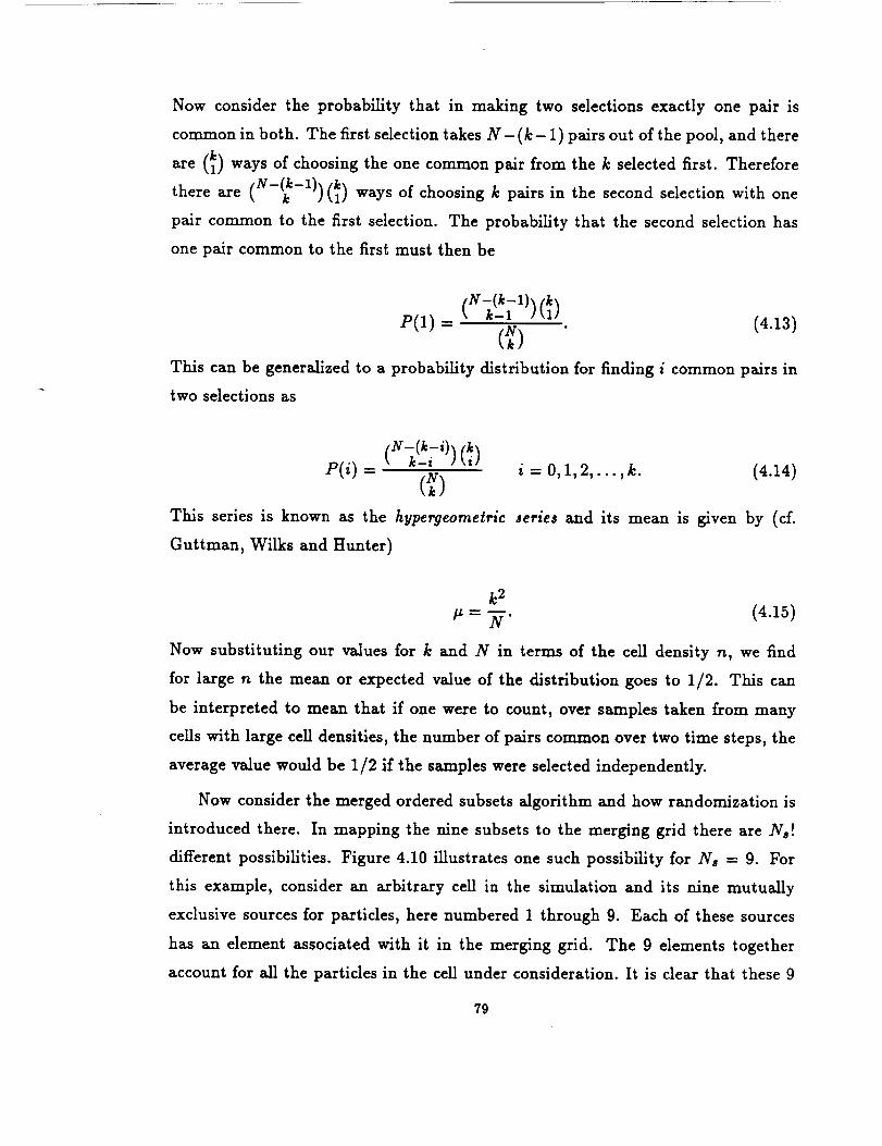
Now consider the probability that in making two selections exactly one pair is
common in both. The first selection takes N-(k-1) pairs out of the pool, and there
are (kl) ways of choosing the one common pair from the k selected first. Therefore
there are (N-_k-1))(kl) ways of choosing k pairs in the second selection with one
pair common to the first selection. The probability that the second selection has
one pair common to the first must then be
P(1) = (N_11))(kl)(N) (4.13)
This can be generalized to a probability distribution for finding i common pairs in
two selections as
P(i) = (N_-i)) (_) i=O, 1,2,...,k. (4.14)
This series is known as the hypergeometric series and its mean is given by (cf.
Guttman, Wilks and Hunter)
k 2
p = _-. (4.15)
Now substituting our values for k and N in terms of the cell density n, we find
for large n the mean or expected value of the distribution goes to 1/2. This can
be interpreted to mean that if one were to count, over samples taken from many
cells with large cell densities, the number of pairs common over two time steps, the
average value would be 1/2 if the samples were selected independently.
Now consider the merged ordered subsets algorithm and how randomization is
introduced there. In mapping the nine subsets to the merging grid there are Ns!
different possibilities. Figure 4.10 illustrates one such possibility for Ns = 9. For
this example, consider an arbitrary cell in the simulation and its nine mutually
exclusive sources for particles, here numbered 1 through 9. Each of these sources
has an element associated with it in the merging grid. The 9 elements together
account for all the particles in the cell under consideration. It is clear that these 9
79

4
7 /
2
J
3
/6
\
3
6
8
1
2
9
5
4
7
ARBITRARY CELL AND ASSOCIATED SOURCES MERGING GRID
Figure 4.10 One possible mapping of nine sources to the merging grid. In this situation, each cell
has at most nine sources for incoming particles which taken for all the cells make up nine mutually
exclusive ordered subsets of particles. There are 9! different possibilities for mapping these sources
to the merging grid.
sources can be mapped to the merging grid through any permutation of 9. By using
a random, statistically independent permutation on every time step randomness is
introduced to the outcome of the ranking. Once a permutation is chosen it is used
in mapping all the ceUs at that time step. In other words the permutation is a front
end array that gets applied in mapping the Ne ordered subsets of particles to the
merging grid.
Unfortunately this does not completely remove the concern with maintaining
statistical independence in even/odd pairings between time steps. Empirical
measurements show that one can expect on average two thirds of the particles
in the simulation to remain in their cells over one time step. Therefore of the Ns
subsets identified as sources of particles in a particular cell, the greatest source is
80

the cell itself. Since the ordering is maintained within each subset, many of the
particles in a cell can be expected to maintain the same neighbors in the NEWS
grid between time steps. This is undesirable since collision candidate pairs are
created from neighboring processors and for the collision selection rule to properly
simulate the fluid mechanics it is absolutely necessary that the pairs created from
the particles in a cell represent a random sample of all the different possible pairs
which could be created.
The number of pairs created in a cell which are identical over two time steps
depends on the particles that leave the cell between the first and the second time
step. As an example consider the case of two particles leaving a cell which contained
a total of four particles. If the two particles which leave were paired together as
collision candidates in the cell, then the two remaining particles also were paired
together and in the next time step, since their order is preserved, these two will
again be paired together in the cell. Assuming as many particles enter the cell
as leave, then half of the pairs created in the cell are identical over two time
steps. Alternatively if the two particles which leave were not a pair, then they must
have been paired with the two particles remaining in the cell. The two remaining
particles, which were not paired together at that time step, will be paired together
in the next time step, therefore in this situation none of the pairs created in the
cell are identical over two time steps. This example can be made more general as
follows. Consider a particular cell, let n be the cell density and let f be the fraction
of particles which remain in the cell over the time step. If all of the particles
which leave the cell were paired amongst themselves as collision candidates, then
of the particles which remain all are paired identically over the two time steps.
Again assuming the cell density is constant over the two time steps, then n f�2
identical pairs are created. Alternatively if among the n(1 - f) particles which
leave the cell none are paired amongst themselves as collision candidates, then
nf - n(1 - f) particles remain which are paired identically over two time steps
leading to n(2] - 1)/2 identical pairs. Typically one can expect a result somewhere
between these two extremes. If f = 2/3, then at worst one third of the pairs are
identical and at best one sixth of the pairs are identical over two time steps.
81

This result is not very encouraging. The additional randomization in the method
comes from reversing the order of enumeration of the particles in each cell and subset
by using the global ending index in computing the rank. The rank is computed by
subtracting the enumeration from this value. If the global ending index is odd, then
evenly enumerated particles will get an odd rank and oddly enumerated particles
will get an even rank. Consequently the pairing of particles, which is done as
even-with-odd, will differ between the two time steps. This must occur on average
in 50% of the cells, therefore for half of the cells the sample of collision candidate
pairs is independent between time steps. Unfortunately, for the other half of the
cells one can still expect between one third and one sixth of the pairs to be identical
to those of the previous time step. This is far more than one would expect for
statistically independent samples.
These results indicate that further randomization is required in this ranking
algorithm. This additional randomization must be applied at two scales. Within
a particular cell, there must be randomization in the order of the particles in each
subset, and there must be randomization of the ordering across the subsets. The
opportunity for accomplishing the first of these exists in the enumeration stage of
the algorithm. The order of enumeration within each subset can be shuffled in a
deterministic fashion at very little cost. The shuffling is performed by re-numbering
the processors in a cell after the regular enumeration has been performed. Two
shuffling algorithms are employed because each shuffling algorithm is deterministic
and two applications of the same shuftIe to a data set produces no change in the
relative ordering. Alternating between two different shuffling algorithms ensures
there is no correlation between samples taken two time steps apart.
Shuffling requires the particle processors to know the subset cell density. This
is obtained through the use of the CM_scan_with_copy instruction. Figure 4.11
has a schematic for each of the two shuffling _gofithms. in the first shuf_ing
algorithm, the processors which previously had an even number are re-numbered
continuously from 1 to n/2 and the processors which previously had an odd number
are re-numbered continuously from n/2 + 1 to n. On the next time step when these
processors are paired as even-with-odd the renumbering will effectively make pairs
82

PARTICLE CURRENT RE- NEWNUMBER NUMBER ORDER
a 1 3 b
b 2 1 d I
c 3 4
d 4 2
SHUFFLE 1
PARTICLE CURRENT RE- NEW
NUMBER NUMBER ORDER
a 1 1 a I
b 2 4 d I
c 3 3 c II
d 4 2 b I
SHUFFLE 2
Figure 4.11 Two deterministic shuffling algorithms. These shuffles are applied on alternating time
steps to the particles in each ceil in order to ensure sufficient mixing.
as even-with-even and odd-with-odd in terms of the addresses in the previous time
step. In the second shuflting algorithm, the numbering of the odd processors is left
intact but that of the even processors is reversed. Therefore if hey is the number
of even processors, then their numbering is changed from from 2, 4, 6,..., 2net to
2ner,27zev - 2,...,2. On the next time step when these processors are paired
as even-with-odd the renumbering will effectively make pairs as £rst-with-last,
second-with-secondlast, and so on, in terms of the addresses in the previous time
step. The reason for two shuflting algorithms should now be clear. If either of
the two shuffles are applied twice in sequence, the resulting pairing is unchanged.
However by ulternating between the two shumes it is possible to guarantee different
pairings for at le_t two succeeding time steps. By the third time step most of the
particles in a cell have left and it is not necessary to worry about correlations over
more than two time steps.
Randomization of the order across subsets must now be addressed. This
randomization is absolutely necessary because the particles within each subset are
highly correlated amongst themselves. Recall that each subset is identified on the
83

basis of the direction of motion of the particles. For example, one subset will include
all the particles which arrived at a new cell from the neighboring cell directly below.
Therefore all those particles will tend to have positive v velocities regardless of how
they are rearranged amongst themselves. Some correlation like this will exist in
each of the subsets. In order to eliminate such correlations it is necessary to mix
the order across subsets.
Of the two shuffles described above, it is clear that only the second one will
allow mixing across subsets. The extension of this algorithm to shuffling across a
complete cell is straightforward; hey becomes the number of even processors for
the cell, as opposed to the number of even processors in a subset for the cell. The
new numbering will then result in pairings between particles of different subsets in
the cell. In a similar fashion the algorithm can be applied separately to the first
and last half of the processors for the cell. By alternating between shuffling over
the complete cell and shuffling the first and last halves separately, the pairing of
collision candidates is made random. The effectiveness of these shuffling algorithms
is investigated in Chapter 7 through calculations for thermal relaxation in a heat
bath and for shock= wave profiles. The results of these calculations could not be
correct if the sample of candidate collision pairs taken from a cell is not random.
4.4.4 When Assumptions Fail
The algorithm has been presented from a physical perspective and in the context
of a generic cell in a generic time step. Two observations of the dynamics of the
simulation were necessary for the algorithm to be valid. It is necessary now to
discuss the situations where these observations do not hold true and the algorithm
cannot be used.
The obvious situation for which the sort wiU fail occurs when particles move
over more than two cens in one time step. The assumption that particles do not
move more than two cell widths in one time step is true to a very high probability,
however given the statistical nature of the simulation it is impossible to rule out the
possibility of a particle not holding to this assumption. Therefore it is necessary to
84

trap such instances and switch to the multi-grid sort when they occur.
A more common situation is for the first observation to fail. The first observation
claimed that the particles go from an ordered to a disordered state through their
motion from one cell to another. This is not true at the upstream boundary of the
wind tunnel where new particles must be introduced to maintain the free stream.
However the introduction of new particles can be delayed an arbitrary number of
time steps, therefore it is convenient to employ the multi-grid sort on those time
steps where new particles are introduced and use the merged ordered subsets sort on
the other time steps. The alternative is to treat the introduction of new particles as
an edge effect and handle it separately. Since the new particles can be introduced
in an ordered fashion the algorithm can be modified to handle this situation by
performing an additional merging. In other words, after ordering the particles in
the flow one introduces the new particles and merges these with the flow particles.
The merging now involves only two ordered subsets and proceeds much faster than
with Na subsets.
4.4.5 Performance and Extension to Three Dimensions
The performance of the merged ordered subsets algorithm depends to some
degree on Ns, the number of subsets to be merged. Na is usually 9, and for this
case the merged ordered subsets algorithm takes about 45% of the time of the radix
rank.
The performance of the algorithm scales linearly with the number of particles
in the simulation. There is also some dependence of performance on Cto¢, the
number of cells, since this number determines the size of the merging grid to be
used. However the fraction of work performed by the merging grid is decoupled from
the fraction corresponding to the particles. Recall that the merging grid is used to
perform one scan and one send operation. The time to perform these operations is
dependent on Ctot and is independent of N, the number of particles. Therefore the
algorithm can be characterized as scaling as O(N + Cto_) although this should not
be interpreted too literally since the time spent by the particle processors relative
85

to the grid processors is dependent on the particular problem.
The algorithm has been presented and discussed for only two dimensions.
The extension to three dimensions is straightforward but does involve a loss in
performance due to increased communications. In three dimensions there are
at most 125 mutually exclusive sets instead of 25. Again one can expect for
the vast majority of time steps only immediate neighbors will act as sources of
particles in a cell, therefore in three dimensions 27 ordered subsets will usually
be identified as opposed to 9 ordered subsets in two dimensions. The algorithm
requires three scan operations with the particle processors per subset. In two
dimensions these operations account for 55% of the time to rank. In the worst
case, in three dimensions that fraction of the algorithm would triple in time so
overall the new ranking algorithm would take about 2.1 times longer than for
two dimensions. In addition, the merging grid would be twice as large in three
dimensions and the time spent by the merging grid would double. Based on
these linear extrapolations it is doubtful that the algorithm would be competitive.
However the above discussion neglects to consider the smaller size of each subset
in three dimensions and the corresponding effect of reduced contention in the
enumeration of each subset. Therefore it is possible that in three dimensions the
algorithm would remain competitive and it should not be ruled out for consideration
until it has been implemented and tested as such.
86

Chapter 5
Implementing General Boundary Conditions
The discussion thus far has focused on the collision of particles amongst
themselves, however of equal importance to a successful implementation of a
particle simulation is also the collision of particles with the surfaces within physical
space. The physics of this class of interaction is not as well understood as one
would hope. Most models for particle-surface interaction assume a perfect crystal
lattice for a scattering surface which interacts with incident particles through some
interactive potential such as inverse power-law or Lennard-Jones (Goodman and
Wachman (1976), Hurlbut (1986)). For purposes of a particle simulation the
exact mechanics of these interactions need not be addressed. As with collisions
between particles, the post-collision thermodynamic state can be sampled from
an equilibrium distribution, however the post-collision position of a particle is
more difficult to define. The situation worsens considerably when dealing with
ablating surfaces. The present work considers only the case of neutral particles
colliding with non-ablating surfaces and makes use of the modes developed by
Woronowicz (Woronowicz and McDonald (1989)). Reference is made to more
complex particle--surface interactions as appropriate.
87

5.1 Representation of Physical Space
5.1.1 Faceted Geometry Approximation
Physical space is represented by the cartesian grid of cubical cells discussed
in Chapter 3. Most problems of general interest involve the flow about some
aerodynamic body, therefore it is usual to set up physical space to simulate a wind
tunnel. Other configurations are occasionally of interest, for example a simple
adiabatic mixer is useful for studying the relaxation of a gas into the equilibrium
state or a standing shock configuration is useful for investigating the internal
structure of a shock wave. These configurations are generally important only for
developing or testing new collision models and have been implemented separately
from the wind tunnel configuration specifically for these purposes.
Surfaces are defined within the grid of cells by planar segments, therefore a
curved surface is approximated by a faceted geometry, as in figure 5.1. This is a
good approximation if the radius of curvature of the surface is much greater than
the dimension of the cell. Therefore in designing a geometry for a specific problem
it is necessary to ensure that a sufficient number of cells are available to accurately
represent the body. This is consistent with the paradigm under which the current
method has been developed, that is one where computationaUy efficient algorithms
allow greater numbers of particles, and therefore greater numbers of ceUs, to be
employed in a simulation.
This faceted body representation was first introduced by McDonald and
Baganoff (1988) and is a useful approximation which allows a great simplification
both in the procedure for identifying particles which undergo boundary interaction
and in defining the interaction for those particles. Each facet is defined by the
equation of a plane
Az + By + Cz + D = 0 (5.1)
such that the unit normal to the plane is then n = (A,B,C) and D is the
displacement of the plane from some origin with a fixed position for all the facets.
S8
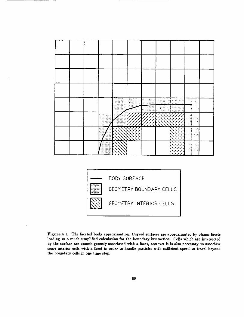
¢sssJ
iiiiii)i .,,,,.........%%%%
• _ s • iill i!
DD
BODY SURFACE
GEOMETRY BOUNDARY CELLS
GEOMETRY INTERIOR CELLS
Figure 5.1 The faceted body approximation. Curved surfaces are approximated by planar facetsleading to a much simpU_ed calculation for the boundary interaction. Cells which are intersected
by the surface are unambiguously associated with a facet, however it is also necessary to associate
some interior cells with a facet in order to handle particles with sufllcient speed to travel beyondthe boundary cells in one time step.
89

Each cell which gets intersected by a body surface must then have associated with
it the parameters (A, B, C, D) representing the surface. It is also necessary for one
or two layers of cells interior to the body to have associated with them these same
parameters in order to capture any particles which had sufficient speed to cross the
surface and travel to an interior cell. All cells associated with the geometry through
these parameters will be termed geometry celIJ. It is a relatively straightforward
procedure to determine which particles have moved behind the surface. For a
particle i lying in a geometry cell the outward displacement, dn, between the particle
and the plane defining the facet is given by
d,, = Azi + Byi + Czi + D. (5.2)
If dn is negative then the particle must have moved behind the surface and the
appropriate boundary interaction must be performed. There exists some ambiguity
when particles have travelled to interior cells in that the the interior cell will be
associated with a single, particular, facet of the surface when in some instances it
may be possible for a particle to have arrived at that cell by crossing a different
facet from the one with which the cell has been associated. However, since the body
surface must have a large radius of curvature with respect to a cell dimension, this
introduces only a small and acceptable error.
A complete body definition must also include values for the fractional cell
volumes, V, of the boundary cells. These must be used to adjust the selection
rule (equation (3.1)) for colliding particles in these fractional cells. Therefore
as a minimum, a body may be defined by a table of the values A, B, C, D, and
V for all the surface cells and interior cells as necessary. For complex three
dimensional bodies the task of determining these values can be carried out using a
method devised by William Feiereisen and described in Feiereisen and McDonald
(1989). On the Connection Machine only two dimensional problems are considered,
primarily because the memory limitations make realistic three dimensional problems
unfeasible. Consequently a full body definition requires only the values A, B, D, and
V to be determined, and in describing the algorithms reference may be made to body
segments instead of body facets.
90

On the Connection Machine the principal problem that must be resolved to
efficiently implement body definitions of this type is again communications related.
The following section describes in some detail how the communications time can
be minimized in a manner that also optimizes the computational effort. The latter
becomes especially important when the surface interactions to be modeUed become
complex.
5.1.2 Storage of Geometry Table
The first issue which must be addressed in implementing this method is the
storage of the geometry table. The problem of storage here is quite different
from the one encountered in implementing the collision algorithm. The tables
necessary for the collision algorithm represent distributions which must be accessed
randomly. Since the collection of particles making up the simulation are themselves
a distribution it makes sense to store the two in the same fashion. In fact the random
motion of the particles is used to help ensure that entries taken from these tables
represent random samples from the distributions. The geometry table, however,
must be accessed in an ordered fashion and this randomizing mechanism is neither
necessary nor useful. For this reason the geometry table must be stored in its own
distinct VP set.
5.1.3 Definition of a Geometry Space
Having decided upon a method of storage for the geometry information, the
question now becomes how to access this information in an efficient manner.
McDonald (1990) describes how this is done in a vectorized fashion in his PSim
code on the Cray 2. In McDonald's implementation all the cells representing
physical space get mapped to a three dimensional array which stores a pointer
to the appropriate entry in the geometry table for each geometry cell and a null
pointer for the rest of the ceils. Therefore to get the geometry information it is
necessary to access this array once for each particle in the simulation to determine
if a particle is occupying a geometry cell and then use the pointers to obtain the
91

appropriate geometry table entry. It would be unreasonable to implement such a
mechanism on the Connection Machine. The communications penalty would be
great due to router contention from all the processors representing particles trying
to access the table of pointers. In order to minimize such router contention it is
useful to define within the simulation space a smaller rectangular subspace which
is just large enough to whoUy contain the body, as in figure 5.2. This subspace is
termed the geometry space and only those particles occupying the geometry space
are considered for boundary interaction. The purpose in defining such a subspace
is to greatly reduce the communications traffic by making use of the fact that most
bodies of interest will occupy only a small fraction of the physical simulation space,
therefore one can easily remove a large fraction of the particles from consideration
for boundary interaction. The only loss in generality is in the assumption of a
wind tunnel configuration. That is, inlet and outlet conditions are hard wired to
simulate a supersonic wind tunnel consequently the code can only be used in such
a configuration. As discussed earlier in this chapter, other configurations are only
of interest primarily in the development of new models and it is not unreasonable
to implement specific codes just for this purpose.
Having defined a geometry space in this manner, it is necessary to map the
geometry in that restricted space. The mapping used here is somewhat different
from that employed on the Cray 2, again a result of reducing communication cost.
On the Connection Machine, indirection can be used to reduce storage requirements
as it is on the Cray 2 only by incurring a performance penalty in communications
cost. If memory is at a premium then the extra cost of the indirect mapping may
be warranted, otherwise it is best to use a direct mapping both for simplicity and
in order to minimize communication cost. The following paragraphs describe first
the indirect mapping and then the direct mapping.
In the indirect mapping, the geometry table is split into two, one table stores
just the cell volumes for the geometry ceils and the other stores the geometry values
A, B, and/9 for the interior and boundary ceils. The two tables are stored in the
same set of processors however indirection exists only for storing the second table
and not in storing the first. Since there are usually less interior and boundary ceils
92

PHYSICAL SPACE GEOMETRY SPACE BODY
Figure 5.2 Definition of physical space and 8eometry space in a wind tunnel configuration.
than there are geometry ceils it is possible to save memory by storing each geometry
value of the second table in a separate processor as in figure 5.3. This assumes that
either the number of geometry cells or the number of virtual processors in the VP
set is at least three times greater than the number of interior and boundary cells,
which generally is a safe assumption given that VP sets cannot be created with VP
ratio less than one.
There is a direct mapping between the cells in the geometry space and the
table storing the cell volumes for these cells. In other words for every cell in the
geometry space there is an entry in a table containing the corresponding cell volume.
Processors representing particles in the geometry space can then access this table
g3 "

directly to get the cell volume. Indirection arises when these processors need to get
the surface geometry values stored in the second table. The pointers to the entries
in the second table can be packed into the same 32 bits storing the cell volume by
sacrificing some unnecessary precision in this value. The cell volume is a floating
point quantity always in the range [0, 1]. Therefore to pack a pointer and a cell
volume into 32 bits it is simplest just to sum the pointer value and the cell volume
together. Then to retrieve the pointer it is necessary only to truncate the packed
result, and to retrieve the cell volume it is necessary only to subtract the retrieved
pointer value from the packed result. The pointer indicates the location of the
first geometry value, A, for that cell. The geometry values B and D are stored in
the neighboring processors as in figure 5.3. The three values may be obtained by
three successive router communication events, however this will triple the router
overhead which for the CM_gst instruction is relatively great. A better procedure
is to temporarily modify the geometry table by letting the processors storing the
A values get the B and D values from their neighbors using two successive NEWS
communication events, and then the three values A, B, and D can be obtained from
a single processor with a single router communication event. Furthermore, if the
number of interior and boundary cells is less than the number of router nodes for the
geometry VP set, it is possible to arrange the second table such that each processor
storing an A value is on a single router node therefore router node contention is
minimized.
In the direct mapping the geometry table is not split, therefore there is a
complete entry with A, B, D, and V for every cell in the geometry space (see figure
5.4). A reflected binary Gray code is used in mapping the table to the processors.
This ensures that table entries are spread amongst all the router nodes thereby
reducing router node contention when the table needs to be accessed. Note that
with the direct mapping there is only a single communication event required to
access the table. Therefore the overhead in starting the communication is paid only
once, hence the communication cost tends to be lower for the direct mapping.
The direct mapping requires more storage than the indirect mapping because
all the geometry cells which are not associated with a boundary must still have
94

!iI iiiili!iiiiiiiiiiii!ili!iiiiiiiiiiii
¸iiiili!iii!iliiiiiiiiiiiiiiiiiiiiiiiiiiiiiiiiiiiiiiiiiiiiiiiiiiiiiiiiii
GEOMETRY SPACE
oFFEEFEEF
F_
F_
F_F_
V
i
!I
I
//
r _' i
i
NULL
B
A
D
B
A
D
B
A
D
B
A
D
B
A
D
B
A
D
B
A
D
GEOMETRY TABLE
Figure 5.8 Indirect mapping between geometry space and geometry table. For every cell in the
geometry space there is an entry in the geometry table storing the cell volume V and a pointer tothe storage location of the rest of the geometry values A, B, and D.
space allocated for the A,B, and D geometry values. However, the difference in
95

storage requirements is not as great as one would think because of the constraint
the Connection Machine has on the minimum size VP set one can create. For
example, the configuration installed at NASA Ames requires a minimum of 32768
(or 32k) virtual processors in a VP set when all 32768 physical processors are used.
Consequently the smallest size table which can be stored must have at least 32k
entries. For the two dimensional problems being considered the geometry space will
usually consist of somewhat less than 32768 cells, therefore for the direct mapping
the storage requirements can be met with 32k x 4 = 128k words. On the other
hand the indirect mapping requires 32k words for the two tables, assuming they
can be fit in a single VP set. Therefore the indirect mapping requires one quarter
the amount of storage necessary for the direct mapping.
The above discussion serves to highlight some of the inadequacies in the Connec-
tion Machine architecture when it comes to storing small tables. In large part the
impressive performance achieved on the Cray 2 in particle simulation calculations
has been accomplished by using tables of pre-computed values wherever possible
in order to avoid performing redundant computation. Clearly for the Connection
Machine to compete there must exist adequate mechanisms for implementing similar
table driven algorithms. Thus far the collision algorithm of Chapter 3 and the
boundary conditions of this chapter have required table look up. Each case required
careful attention to the manner of storage in order to minimize the cost of access.
Each resulted in a very different manner of storage but common to both was a
tradeoff of memory for communications performance. Consequently in both cases
the storage requirements were greater than that demanded by the table.
The observations made in the preceding paragraph help substantiate a more
general statement one can make about the Connection Machine, namely that
memory requirements for algorithms implemented on the Connection Machine
are generally greater than for the same algorithms on vector machines. This is
clue in part to the tradeoff between memory and communications but is more
accurately prescribed to an inherent characteristic of the architecture. An example
of this is manifest in the minimum table size requirement described above, but the
implications are more general. Consider that the allocation of temporary space is
96

A B D V
_! ii! _ i!. i!ii!_ ii !iiii!!i!_
GEOMETRY SPACE
GEOMETRY TABLE
Figure 5.4 Direct mapping between geometry space and geometry table. For every cell in the
geometry space there is an entry in the geometry table storing the values A, B, D, and Y. The
geometry table is stored in its own VP set which, due to the minimum size restriction on VP sets,
often will be much larger than the table. Table entries are spread amongst all the router nodes byuse of a reflected binary Gray code mapping.
97
effectively equivalent to creating a table, therefore the minimum size temporary
space which can be allocated is 32768 bits, in other words one bit al]ocated in
each virtual processor of the smallest size VP set one can create. In reality the
situation is worse because rarely can one use only a single bit of temporary space
per processor and rarely is one operating in the minimum size VP set. In a particle
simulation it is often necessary to allocate temporary space in the VP set storing
the particles. This VP set may have over two million virtual processors in which
case allocating a single word of memory in each processor leads to 2M words (that
is 8 MB) of temporary space. Note that all this space must get allocated even if
not all the processors are active for the calculation which requires the temporary
space. This is due to the $IMD nature of the Connection Machine and cannot
be avoided. All the processors in the active VP set must receive and be able to
execute the instructions issued from the front end computer, therefore reference to
memory locations within a processor must be identical for all the processors (since
these must be part of the single instruction issued by the front end) consequently
there can be only one stack pointer for all the processors in a VP set. The next
section examines how these restrictions can be circumvented in some situations by
spawning slave VP sets of smaller size.
5.1.4 Master and Slave VP Sets
Once the geometry space has been defined and the processors representing the
particles within it have been identified, it seems the next logical step would be
to have those processors get the geometry information from the geometry table
and then carry out the necessary calculations. It is not immediately obvious why
one would want to carry out the calculation with a different set of processors
since that would introduce additional communication. However, this situation is
analogous to sampling macroscopic quantities (see section 3.4) in that the total cost
in communication can be reduced by initiating the communication from a smaller
VP set. The reason for this has to do with the way instructions are carried out by
the Connection Machine. Recal] that instructions are issued from the front end and
98
sequencedto a set of virtual processors. Virtual processors are created from the
physical processors by allocating physical processor memory in equal amounts for
each virtual processor and then looping through the microcode of a given instruction
once for each virtual processor. The important point to realize is that the loop is
carried out even if the virtual processor is not active for the instruction. Therefore
in general the cost of executing an instruction increases linearly with VP ratio
regardless of the number of processors active. The most obvious exception to this
rule is in the case of router communication where router network contention is
reduced when less processors are sending messages, however from figure 2.3 it is
clear that this has a second order effect on performance compared to reducing the
size of the VP set. In the current situation we have isolated a relatively small
number of processors in a very large VP set which need to get information from
processors in a different VP set. Clearly there is a huge penalty to be paid if this
operation is performed from the large VP set since most of the processors there
will be inactive. The better solution is to create a separate VP set, which here
will be called the slave VP set, just to accommodate the necessary data from the
active processors and then perform these operations from there. The larger VP
set for which the operations are to be performed naturally is called the ma_ter VP
set. The slave VP set becomes a useful mechanism for improving performance only
when there is a relatively large disparity between the VP ratio of the master and
the slave VP sets. If this is the case then the cost of sending information from the
master to the slave can be more than recovered.
Given the considerations of the preceding paragraph, the algorithm for com-
puting the boundary interactions is as follows. A slave VP set just large enough
to accommodate all the particles in the geometry space is created. The processors
representing the particles in the geometry space then send their self-address and
the cell index of their particle to the appropriate processor in the slave VP set. The
sending processors here are in the master VP set, and the particle information in
the master VP set is in the rnaJter table. The self-address of a master processor is
actually the minimum required by the slave for it to proceed, however in the current
context the next step for a slave would be to get the cell index from the master,
99 _

therefore it proves more efficient for the master to send both the self-address and
the cell index in one package. With this information the slave processors can then
proceed to get the geometry information from the geometry table. The pattern of
communication here will depend on the method of storage for the geometry table,
that is whether there is an indirect mapping or a direct mapping of the geometry
table. The preceding section described the method of access in both cases. From
the geometry information, specifically from the cell volume, a slave processor can
determine if its particle is occupying a boundary or interior cell. Such particles
must be checked to see if they have crossed into the body and must be reflected
back into the flow. This requires the slav-.- processors to get the position and velocity
components from the master table and then apply equation (5.2). The manner of
reflection depends on the type of surface being represented.
Three different types of surfaces can be represented corresponding to inviscid,
isothermal, or adiabatic boundary conditions. The methods for simulating these
types of surfaces are discussed in the next section therefore the details will not be
described here. Essentially, for those particles which do undergo surface interaction
the slave processors must get more information from the master table and possibly
from the geometry table as well, perform some calculations, and then return the
updated position and velocity information to the master table. The final operation
which the slave processors must perform is getting the new cell volume for those
particles which changed cells after reflection. This information along with the
updated position and velocity for the reflected particles is returned to the master
table. This ends the algorithm, the memory of the slave processors can now be
deallocated and the slave VP set can be destroyed.
5.2 Models for Particle-Surface Interaction
In this section three models for particle-surface interaction are discussed; they
correspond to simulating inviscid, isothermal, and adiabatic boundary conditions.
100

5.2.1 Specular Reflection
The simplest surface interaction to model is specular reflection of a particle
from a stationary surface. Specular reflection is defined such that the angle
of incidence is equal to the angle of reflection, as in figure 5.5. No energy is
exchanged between the particle and the surface nor is the tangential velocity of
the particle affected, therefore this type of interaction is suitable for simulating
inviscid boundary conditions. Typically only the wind tunnel walls are treated as
inviscid but for validation purposes it is useful to compare simulation results to
theory, in which case simple bodies (such as the two dimensional wedge) may also
be treated as inviscid.
The only information necessary to perform the specular reflection of a particle
from a plane surface is the definition of the plane itself. A particle i lying a distance
dn behind a plane with outward unit normal ns will be reflected as
xti = xi - 2dnns.
The velocity will be reflected as
(5.3)
vts = vi + 2(ns-vi)ns. (5.4)
Equations (5.3) and (5.4) can be generalized for the ease of a non-stationary
surface. Such a situation is of interest primarily for the development of general
entrance and exit conditions in a wind tunnel simulation although it can also be of
interest in the study of flow over a body in motion.
To generalize (5.4) it is necessary only to substitute the relative velocity Vrel, i
between the particle and the surface, therefore
where
Vts = vi + 2(ns • vrel,i)ns (5.5)
Vrel, i -- vi -- vs (5.6)
101

vi
Oi
n$
I
dnOi Or I
Figure 5.5 Specular reflection of a particle from a stationary plane.
and vj is the velocity of the surface.
The generalization of (5.3) is not quite as straightforward. It is necessary to
consider the time step in two parts, that is the time before interaction and the time
after interaction. The time before interaction, t/r/is just the time for the particle to
have moved from its initial position to its intersection with the surface. Therefore
tb/ = n,-(x, -- xi) (5.7)ns- (v, -- vi)
where xs is any point on the surface. The new particle position must be given by
advancing the old position for a time tbi at tlae pre-interaction velocity v i and for
time At - tbi at the post-interaction velocity v_i . In other words,
x¢i = x i + tbiv i + (At -- tbi)vri
where At corresponds to a full time step. Combining with (5.7) this becomes
(5.8)
102

= + tv, + 2n, . (AtC,r - ,,,)- + x,))no. (5.9)
5.2.2 Diffuse Reflection With Surface-Driven Energy Exchange
The diffuse reflection of a particle from a surface represents a more realistic
kind of surface interaction. A diffuse reflection is defined as one where the
post-interaction velocity is independent of the pre--interaction velocity, conse-
quently the post-interaction velocity must be sampled from some distribution. It
can be proved theoretically (cf. Wenaas (1971)) that in equilibrium the diffuse
scattering of particles from a surface must obey the cosine law. The cosine law states
that particles striking a surface element will scatter with intensity proportional to
cos 0a regardless of the angle of incidence, where 0s is the scattering angle measured
from the surface normal. Note that this law does not state that particles leave a
surface in random equally weighted directions but rather the directions are weighted
by a factor of cos 0a. This is the result of biasing the equilibrium distribution to
include only those particle which have crossed the plane represented by the surface.
In other words, the cosine law can be arrived at by assuming that in thermal
equilibrium the velocity distribution of particles leaving a surface is identical to
that of particles arriving at the surface, both of which are distinct from the velocity
distribution of the gas as a whole.
From the above discussion it is clear that the post-interaction velocity of
a particle undergoing diffuse reflection can be arrived at by sampling from an
equilibrium distribution and accepting only a result which directs the particle away
from the surface. Alternatively, one can accept any sample from an equilibrium
distribution but reverse all the components of a result which directs the particle
back into the surface. The question remains as to the temperature of the equilibrium
distribution to be sampled. If this value is fixed for all particle-surface interactions
then the energy exchange between the particles and the surface can be considered
surface-driven and the boundary condition is isothermal.
103

In the current context, the post-interaction velocity can be sampled directly
from the thermalizer particles. As described in Chapter 3, particles which are not
in the flow are kept in a separate reservoir, or thermalizer, and are allowed to collide
amongst themselves. These thermalizer particles represent an equilibrium gas,
therefore to sample a post-lnteraction velocity for diffuse scattering it is necessary
only to use the velocity of a randomly selected thermalizer particle. The therma]Jzer
is kept at the free stream temperature, consequently to simulate a surface at some
arbitrary temperature it is necessary first to scale the therma_zer particle velocity
by a constant factor equal to the square root of Tj/To where Ta is the surface
temperature and To is the free stream temperature.
Unfortunately, there is no law similar to the cosine law for determining the
post-interaction position of the particle. Currently the post-interaction particle
position is defined by
xli --xi - dnna (5.10)
which is similar to equation (5.3) but always places the particle directly on the
surface. Woronowicz and McDonald (1989) report some flow fieldsensitivityto
the placement of the particleafter boundary interaction,which isnot unexpected
given the direct influence this has on the boundary layer. Placing the particleon
the surface is equivalent to assuming that the surface interaction time is on the
order of a time step. This isnot a good assumption and it ismore likelythat the
surface interaction time is on the order of the collisiontime which is much less
than a time step. The alternativethen is to place the particle somewhere in the
flow, consistent with assuming a short surface-interactiontime. However this too
is less than satisfactory. Consider that the post-interaction velocity must direct
the particleaway from the surface (a necessary restrictionto satisfythe cosine law)
therefore placing the particle away from the surface has the effectof creating a
vacuum rightat the surface which isalso undesirable. The issueisfax from resolved
and is in an area which clearlydeserves further investigation. Nonetheless (5.10)
does seem to reproduce satisfactoryresults and is currently used for all diffuse
reflections.
104

5.2.3 Diffuse Reflection With Gas-Driven Energy Exchange
The third type of surface which can be simulated is adiabatic and is defined as
allowing no net heat flux across the boundary. The specularly reflecting surface is
a very restricted example of an adiabatic boundary condition in that no energy is
transferred into the surface, however the reflection is not diffuse. The more general
case must have diffuse reflection and allow energy transfer into the surface on an
individual basis but such that over many interactions there is no net energy transfer.
The approach described in the previous section cannot be applied here because the
surface temperature is not fixed or known a priori. The surface temperature is
dependent on the state of the gas at the boundary, therefore the energy exchange
between the particles and the surface can be considered gas-driven and requires a
different approach to specify.
The approach taken here was first proposed by Woronowicz and McDonald
(1989). In this method a boundary particle is created to represent the surface, then
when particles interact with the surface they do so by undergoing a collision with this
boundary particle. The coUision is inelastic in the sense that the internal energies
of the particles are allowed to participate in the energy exchange, however total
energy is conserved over the coUision. The surface is always in thermal equilibrium
with the gas therefore the surface temperature win equal the gas temperature and
there can be no heat flux into the surface. However the boundary particle will
tend to acquire a net momentum from repeated collisions with flow particles which
are always directed into the surface. This problem is alleviated by restricting the
motion of the boundary particle to a cubical ceU. This is accomplished simply by
permuting the boundary particle velodty components after each collision and there
is no need to trace the particle's position.
It is important to note that the model, as described thus far, allows only a single
temperature for the entire surface represented by the boundary particle. In other
words there is perfect thermal conductivity in the surface. Initial investigations
with this model concentrated on the flow over a wedge and used a single particle
to represent the whole wedge. It was found that the rear of the wedge acquired the
105

same temperature as the face and therefore had a stronger influence on the wake
flow than ought to have been the case. The obvious solution for such a situation is
to have two boundary particles, one for the face and one for the rear of the wedge.
Since the flow over a wedge is conical the face will acquire a single temperature and
a single boundary particle can be used to represent this surface. However, more
general geometries cannot be represented as simply and in the most general case
one would require a boundary particle for each cell of the surface. This is the model
implemented on the Connection Machine.
On the Connection Machine there exists a boundary particle for every cell
associated with the surface. The particle is monatomic therefore only the three
translational velocities need to be stored. These are stored in the same VP set used
to store the geometry information and again a binary reflected Gray code is used to
ensure that the particles are spread evenJy amongst all the router nodes for optimal
communication. The boundary particle information is accessed by the slave VP
set after the slave processors have determined which flow particles must undergo
surface interaction. At this point the appropriate slave processors get the boundary
particle information and perform a strictly elastic collision between the monatomic
boundary particle and the flow particle. The update boundary particle state is
then returned to the geometry VP set. Note that all the particles in a particular cell
that undergo surface interaction are made to collide with a boundary particle which
is in the same state for each collision. After collision with the flow particles only
one updated state is actually returned to the boundary particle, in other words
only one surface interaction in a time step is allowed to change the state of the
boundary particle. This imposes a small restriction on the influence a single surface
interaction has on other surface interactions in that time step. For a given time
step and in a given cell all the surface interactions are carried out independent of
each other and the result of one interaction does not affect any other for that time
step. Consequently the amount of energy exchange between the surface and the gas
over one time step is more restricted than it would be if each surface interaction
in a cell were carried out sequentially and thus allowed to influence the state of
the surface for all succeeding interactions. However this is a small and therefore
106

acceptable restriction since the actual number of surface interactions in a cell is
small and since the particles in a cell are all in a similar state. In fact gradients
cannot be supported across a cell and the particles in a cell can be considered to be
in thermal equilibrium therefore it is not strictly necessary to allow a dependence
between particle-surface interactions within a time step.
107

Chapter 6
Active Flow Visualization
Through the I/O Subsystems
The capability of transmitting at high bandwidth to I/O subsystems is a feature
of the Connection Machine which allows the investigation of transient or unsteady
flows. In particular, the DataVault can be used to save the solution throughout
the transient or unsteady phase, and the frame buffer can be used to visualize the
solution either in real time or as play back from the DataVault. The performance
penalty in carrying out these operations during the calculation is minimal because
the links to these I/O subsystems are of very high bandwidth. This chapter
discusses the visualization technique employed with the particle simulation and
various strategies for applying this technique in the investigation of transient flow
phenomena. Finally, the extension of this technique to three dimensional flows is
described.
6.1 Visualization Technique
6.1.1 Mechanism for Visualization
The particle simulation method is particularly appealing to visualize because
108

the calculationis tied closelyto the actual gas dynamics. The mechanism for flow
visualizationin realtime and as play back isthe same. Each particleisrepresented
by a colored pixel in the display,therefore the motion of the particlesisseen in the
corresponding motion of the colored pixels.
This mechanism for visualizationis unique in the quantity of information that
can be assimilated by the viewer. Density in the flow isimmediately visiblethrough
the concentration of painted pixels in the display. Similarly,the velocity fieldis
visiblein the motion of the painted pixels in the display. Therefore there is a
directcorrespondence between the number density and velocityin the flow and the
painted pixel density and motion in the visualization. Furthermore, it ispossible
to concurrently visualizeanother thermodynamic variable,such as temperature or
pressure,by mapping itto a color scaleand applying thisscalein painting the pixels.
Such thermodynamic variablesrepresent macroscopic flow quantitiesgenerated from
the particledistributionswithin the cells_thereforewithin a cella singlecolor value
is representative of all the particles. The color of a particle in the visualization
corresponds then to the value of the macroscopic flow quantity in that region of the
flOW.
The limitation in this mechanism usually liesin the resolution of the display
device. Typically one can expect no more than 106 pixels to be available for
the display such that in a simulation space of 256 x 256 cellsone will have a
resolutionof 16 pixelsper cell.In a simulation involving2.0x 106 particles(currently
the greatest number possible on the Connection Machine available through the
Numerical Aerodynamics Simulation facilityat NASA Ames, although one would
expect this number to be as high as 16 x 106 on a 64k processor machine with a
memory upgrade)]t becomes impossible to resolvethe individual particlesifallare
to be displayed. Therefore itisnecessary to display only a fractionof the particlesin
order to visualizetheir motion and concentration. By displaying every k th particle
in the list(/cbeing some suitably large integer),one can stillvisualizethe density
and velocity fieldalthough not allthe particlesfrom the simulation are displayed.
109

6.1.2 Implementation of Visualization Mechanism
The implementation on the Connection Machine of this mechanism for flow
visualization with a particle simulation makes use of the frame buffer. The frame
buffer allows dynamic displays of size 512 x 512 or 1024 x 1024. Naturally the
greater resolution display will require a corresponding greater number of virtual
processors, and therefore memory. The lower resolution display is useful when
memory Limitations rule out the greater resolution or when the visualization is to
be recorded on video tape for play back at regular network tdevision resolution
(NTSC format).
The geometry is displayed on the overlay buffer. Since the geometry is static
there usually is no need to redraw the overlay buffer during the visualization.
Nonetheless redrawing the overlay buffer during the visualization normally is fast
enough that it does not affect the animation of the flow. Therefore the overlay
buffer can also be used to display changing statistics in the simulation. For example
a dynamic "time bar" can be used to display the current time step or one may want
to display other scalar information such as peak temperature in the flow, total heat
loading on the body or Lift and drag for the body. If the overlay buffer is to be
used dynamically in such a manner then it is necessary to save the static portions
to avoid recomputing the display. This is especially true when text is involved since
fonts are bit mapped and font calculations are carried out on the front end at a
tremendously slow rate by comparison.
The particles are displayed on the RGB (Red/Green/Blue) buffers. These can
be configured as a single 24 bit color buffer or as three separate 8 bit color buffers.
With the current technique 24 bit color is unnecessary since the eye is uncapable of
grasping such a broad palette of colors in a dynamically changing display of moving
particles. Therefore it is better to employ 8 bit color thereby saving memory at
a rate of 16 bits per pixel. For a static display 24 bit color may be useful for
enhancing the visualization of density while letting all the particles be displayed.
In such a case instead of using RGB values to map the colors one would use HLS
(Hue/Lightness/Saturation) values, letting the hue and lightness determine the
.¢
110

color corresponding to the desired thermodynamic quantity for particles in a cell
while letting the saturation give some idea of the number density. The color scale
would then be two dimensional, with the mapping for the the displayed quantity
given along one axis and the mapping for the density along the other.
With 8 bit color one has three separate color buffers for the display. It is
possible to write to any of these three buffers, however only one buffer can be
displayed at a time. Because changing the displayed buffer is always faster than
writing to the buffer, animation is performed on most graphics systems by writing
to an undisplayed buffer and switching with the displayed buffer once the writing
is completed. This technique can be employed on the Connection Machine as well
although, as was mentioned in describing the use of the overlay buffer, the writing
to the buffer proceeds faster than the eye can respond therefore it is unnecessary
to employ such a strategy.
Writing to the frame buffer is similar to communicating to a separate VP set. To
display the particles in the frame buffer, the VP set storing the particle information
must send an 8 bit color value to the frame buffer for every particle which is to be
displayed. If only a fraction of all the particles are to be displayed, it is advantageous
to use field aliasing (as discussed in Chapter 2) to reduce the VP ratio and speed the
communication. If the color value is to correspond to a thermodynamic quantity,
then that quantity must first have been sampled from the simulation and the result
must have been mapped to an 8 bit integer in all processors which are to display
their particle. Note that this additional calculation and communication takes less
than 5% of the total computational time.
6.2 Visualization Strategies
6.2.1 In Real Time
In real time the technique described in the previous section is used for visualizing
the calculation as it proceeds. This can be of tremendous use for debugging code
III

as weU as for evaluating new geometries. As a debugging tool clearly it is useful
for identifying how the data is becoming corrupted. Often bugs in the program are
evident in the strange behavior of particles or unrealistic temperatures for the ceUs.
This kind of information is immediately available from a real time visualization and
can be used to identify the source of error.
In describing a new geometry it is necessary to ensure that particles do not leak
through the body and that the body is having the desired effect on the flow. Any
unexpected effect that the body definition may have on the flow becomes evident
through the visualization. In applying the simulation method to a new geometry it
is also necessary to make some estimate of how many time steps will be necessary to
reach steady state. Again this is information that is immediately available from a
real time visualization. In other words, one can see through the visualization when
the shock structure has become fully developed and the flow has reached steady
state.
6.2.2 Through Play Back
The idea behind using play back visualization is both to speed up the display of
information and to have a stored solution which can be viewed repetitively without
repeating the initial calculation. The limitation one encounters is finding sumcient
storage for the solution. If there were truly infinite storage devices, one would then
store all the particle information for every time step and thus be able to completely
recreate any aspect of the simulation in the play back. Unfortunately, at 28 bytes
per particle (in two dimensions) and two million particles that requires 56 MB per
time step or about 6 GB per 100 steps. Clearly this is unfeasible for visualizing
transient flows over several thousand time steps.
An alternative is to store only the information sampled from the ceils. At a
minimum, one would store the number density, the u and v velocity components,
and the translational temperature. This would require 16 bytes per cell or 1 MB
per time step for a simulation with 64k cells. This is feasible in terms of the storage
requirements, however the visualization now loses those appealing aspects described
112
in the first section. In other words, the visualization would now proceed in either of
two ways. One would visualize the changing macroscopic quantities such as density
or temperature by displaying those fields with a suitable color map, or one would
visualize the changing velocity field using tracer particles in a manner analogous
to the visualization techniques used with regular CFD solutions of transient flows.
However, it is no longer possible to visualize both the thermodynamic quantities
and the flow field simultaneously.
There are two alternative strategies one can use in order to retain the
visualization technique described in the first section while using a feasible amount
of storage. The first of these strategies is simply to save each image of the flow as
it is created in the real time visualization. For a 1024 × 1024 display this requires
1 MB per time step regardless of the number of particles or the number of cells
employed. Although this scheme retains all the unique features of the particle
simulation visualization technique it suffers from a lack of flexibility in the choice
of displayed information. In other words, one has to decide ahead of time on the
quantity to be displayed and the color map to be used. This requires running several
smaller scale simulations with real time visualization to arrive at a suitable display
for the full scale solution. If one later finds not all the necessary information has
been captured, it becomes necessary to repeat the calculation.
A more robust scheme is to combine the two previous strategies, that is, saving
the sampled information and saving the display. By eliminating redundancies in the
information the storage requirements can be reduced to le_J than that necessary
in applying either strategy individually. As a minimum one saves the sampled
density, the temperature, and the flow speed for the cells. From the density and
the temperature any other equilibrium thermodynamic quantity can be computed,
and from the temperature and the flow speed the Mach number can be computed.
For a grid of 64k cells these three quantities will require 768 kB of storage per time
step. In addition to this, in order to visualize the particle motion in the flow just a
bit map of the display is stored. Since the smmpled flow information will be used to
to color the particles it becomes unnecessary to save the color used in the real time
display. Storing a bit map of a 1024 x 1024 display requires 128 kB, therefore in total
113
896 kB per time step are required with this scheme. To produce a display the bit
map is used to identify the pixels which need to be painted, and the saved solution is
used to select a color. This scheme has the advantage of saving the actual solution,
as opposed to the displayed visualization. For this reason the scheme allows great
flexibility in recreating the simulated flow. It is possible to visualize any desired
quantity through an appropriate color map, therefore different reproductions of
the simulated flow can be created in order to investigate the behavior of different
quantities throughout the solution.
The design of a good color map is not a trivial matter. When the color is to
be used to display a thermodynamic quantity it is necessary to know the range of
variation for that quantity and ensure that there is good contrast between adjacent
colors in the map throughout that range. The range of variation may change
dramatically with free stream Mach number and a single universal color map is not
possible. With the play back visualization one can tailor individual color maps for
each displayed flow quantity to produce the best effect for the particular geometry
and flow conditions being simulated.
6.3 Extension to Three Dimensions
The discussion thus far has been restricted to the visualization of two dimen-
sional flows. Eventually it is desired to apply this technique to three dimensional
flows, therefore it is appropriate to address the question of the changes required in
the visualization technique. It is clear that one could not simply display the entire
flow as an isometric projection without adjusting the size of the displayed particles
to reflect depth in the flow. In theory this would give a correct representation of
a three dimensional flow, but in practice one would almost certainly find that the
resolution of the display device would prove to be a limitation. The experience
obtained in displaying two dimensional flows indicates that four pixels per particle
is the coarsest resolution one can use without defeating the purpose behind using
colored particles to visualize the solution. Even at a pixel per particle one has to
114
make compromises in the number of particles displayed, therefore the display device
already is a limitation in the visualization of two dimensional flows.
It is evident that the technique can be applied only to the two dimensional
planes making up a three dimensional flow. The issue then becomes how to convey
the three dimensional information in a two dimensional medium. This could be
best accomplished by allowing fast switches between planes in the simulation.
In other words, the displayed plane could be allowed to change rapidly under
user control thereby allowing the user to investigate the third dimension of the
solution in whatever manner desired. In a two dimensional visualization user input
is not necessary because people are accustomed to two dimensional displays and
generally have similar responses to information conveyed in this manner. This
is not true of three dimensional information where the response will vary greatly
from person to person. Therefore it is important for the visualization of three
dimensional information to be under the control of the viewer. In such a scheme
it would be necessary to aid the viewer in grasping which plane is being displayed.
For this purpose the overlay buffer could be used to display the entire three
dimensional geometry in isometric projection while the particles corresponding to
a two dimensional slice of this geometry would be displayed.
Naturally the storage requirements of a three dimensional flow visualization are
much greater than for two dimensions. In three dimensional simulation with 64k
cells in the two dimensional plane one would require 896 kB per plane per time step.
With 50 planes in the simulated space one requires 44 MB per time step. Therefore
storage limitations make it impossible to save a full transient solution, however the
technique could be very useful for visualizing the steady state three dimensional
solution. For the steady state one need save only the time averaged solution, not
the transient solution at each time step. The steady state solution in this example
would require 12.5 MB per sampled quantity. The bit map information for one time
step would require an additional 5.3 MB. Therefore three sampled quantities and
bit maps for 10 time steps would require only 91 MB of storage. The visualization
would proceed by looping over the 10 bit maps to display the particle motion while
using the saved solution to decide on a color for each particle. The user would
115

control which plane is displayed and what quantity is used to color the pixels. The
entire 91 MB of information could be loaded into 16k processors so the visualization
would proceed at a very fast rate entirely from the Connection Machine.
116


Chapter 7
Results
The algorithms presented in the previous chapters are now applied to several
example problems in order both to validate the algorithms and evaluate the
performance of their implementation on the Connection Machine. The first problem
to be examined is the relaxation of the internal degrees of freedom in a diatomic
gas. Results are compared to solutions computed with McDonald's code on the
Cray 2. The second problem to be examined is the structure of a normal shock wave.
Again results are compared to solutions computed by McDonald. Finally, a large
two dimensional solution is presented for the flow field about a proposed geometry
for the Hermes Space Shuttle to be built by the European Space Agency. This
solution is used to demonstrate the capability of the method for solving hypersonic
flow problems of practical engineering interest and is also used to evaluate the
performance of the Connection Machine in comparison to the Cray 2 for a general
two dimensional problem.
7.1 Relaxation of Internal Energy Modes
To test the the nonequilibrium temperature model, the relaxation of a diatomic
gas to its equilibrium condition is examined. This simulation uses the adiabatic
117

box configuration with gas molecules initialized to a nonequilibrium state. The
energy exchange resulting from collisions of the particles eventually relaxes the
gas to equilibrium. In addition to providing a useful check on the nonequilibrium
temperature model, this simulation provides a particularly severe test of the
randomization algorithms incorporated to the merged ordered subsets sorting
algorithm. The aim of these randomization algorithms is to make the deterministic
"even-with-odd" pairing of collision candidates result in a statistically random and
uncorrelated sample of colliding pairs. Since multiple collisions of the same pairs are
effectively equivalent to a single collision, if the pairs in a sample are correlated to
those of the previous sample then the effective collision frequency is reduced. The
result manifests itself macroscopically as a reduced relaxation rate and produces
an incorrect equilibrium division of energy between the various modes. The latter
occurs because the temperature model assumes a particular energy distribution for
the set of colliding particles and redistributes the collision energy based on this
distribution. If the collision rate is incorrect then the set of coUiding particles will
also have an incorrect energy distribution and the correct equilibrium division of
energy is not obtained.
Figure 7.1 presents the results for relaxation from three different initial
temperatures and compares these to the same simulations performed by McDonald
on the Cray 2. In all cases the agreement between the two is excellent. It should also
be noted that these results are in agreement with results from DSMC calculations
performed by Boyd for the same problem (McDonald (1990)). The collision numbers
were fixed at Z,-ot = 5 and Zvi b = 50. The simulations employed a hard sphere
interaction potential with diatomic molecules having two rotational degrees of
freedom and a characteristic temperature for vibration corresponding to molecular
nitrogen, Ovi b = 3390°K. The Connection Machine results are represented by the
solid lines in the figure and the Cray 2 results are represented by the 'o' symbols.
The initial nonequilibrium condition was for all the energy to be in translation
leaving no energy in rotation or vibration. Figure 7.1a is the result for an initial
translational temperature of To = 273.15°K. For such a low reference temperature
one can expect essentially no excitation of vibrational states in the gas, and the
118

Z
IJ
0.9
0.8
0.7
0.6
0.5
0.4
0.3
0.2
0,1
G0
0.9
0,8
0.7
0.6
0.5
0.4
0.3
0.2
. 4 .d.q7r .;_4._.,e oooe_o._oo.9 -_-q_...o. - o-t-_oe-.-4_o-,_ .._-..e.. - - qr o- ._,* -
ef_ ........... + ...................
d"
8 ...... '.............................
50 I00 150 200 250 300 350 400 450 500
.! ........ : ............... (b)2 ........... ......
0.1 o.oo O.o,.ox,po_o4_80 Q* ooo all'o* ° ° °° _Q a*°c ° Q°a ° ° _ _° _° ° °°
ooO _e°0 _ * ' '
200 400 600 800 1000 i200 1400 1600
0.9 ...........................................................................
0.8 ....
0.'7
,,_ 0.6
: o o,o oo o lltD0 0 _°O+Oe e_" -
0.2 ooO o°._'° e °
o •0+I o °+ .....
oo
o00 200 400 600 800 tO00 1200 1400 1600
Figure 7.1 Relaxation of internal degrees of freedom in a diatomic gas with fully excited rotational
energy and a characteristic temperature of vibration of 3,390°K. Results are for three initial gas
temperatures with only translational energy present a) 273.15°K, b) 3,390°K, c) T --+ o_. Symbols
are used for current results and lines represent the calculations by McDonald (1990). -- E,,; ....
Erot ; • • • .E,_ib1!9 -

energy exchange is primarily between translational and rotational modes. For 3
translation degrees of freedom, 2 rotational degrees of freedom and no vibrational
equivalent degrees of freedom one expects an equilibrium division of energy of 60%
in translation and 40% in rotation, as is observed in the figure.
Figure 7.1b is the result for an initial translational temperature of To = 3390°K
which is exactly equal to the characteristic temperature of vibration. This represents
a situation where the vibrational state is only partially excited. It is possible to
calculate the theoretically expected equilibrium division of energy between the
various modes by considering conservation of energy. Conservation of energy
requires
3
err + e,ot + e ib = 5RTo. (7.1)
Assuming translation and rotation are both fully excited and using equation (3.28)
for vibration, then
err = 3 RT
erot = 2 RT
ROvib (7.2)%ib = ezp(O_/T) - 1
Substituting (7.2) in (7.1) yields a transcendental equation in T which when solved
numerically for this particular case results in a final equilibrium temperature of
T = 1790°K. This corresponds to an energy division of 53% in translation, 35% in
rotation and 12% in vibration as is observed in the figure. Therefore the simulation
is producing the correct equilibrium result.
Figure 7.1c is the result for an initial translational temperature approaching
infinity such that the ratio Ovib/T approaches zero. This is the limiting case for
which vibrational energy becomes fully excited with two full equivalent degrees of
freedom. At equilibrium there is an equal division of rotational and vibrational
energy as is observed in the figure. Evident in this figure also is the rotational
120

energy overshoot due to the great difference in the relaxation rates of vibration and
rotation.
In all three cases the agreement with the Cray 2 results is excellent. This not
only is a validation of the nonequillbrlum temperature model as implemented on
the Connection Machine but also is a validation of the randomization algorithms
incorporated into the sorting. These results indicate that the simulation is creating
and maintaining the correct distribution functions for the particles. The next section
further validates the current implementation by examining the temperature and
density profiles across a normal shock wave in an ideal diatomic gas.
7.2 Normal Shock Wave Structure
Accurately predicting the internal structure of a shock wave is a prerequisite
of any valid particle simulation. The shock wave represents a region of highly
nonequillbrium flow connecting two different equilibrium states. This is a much
more complex problem to study than the relaxation of a gas because the molecules
undergo convective processes in addition to diffusion. This also is an important
test for a particle simulation since the shock wave problem represents an area
where particle methods historically have provided the only accurate computational
solutions. Continuum methods employing the Navier-Stokes equations produce
incorrect results for the internal structure of a hypersonic shock wave and efforts
at extending the continuum approach has focused on the solution of the Burnett
equations. Only recently (Lumpkin, Chapman and Park, (1989)) have these been
shown to provide reasonable solutions for shock wave profiles.
With the addition of bulk motion to the gas it becomes necessary to properly
simulate entrance and exit conditions for the molecules. Proper entrance conditions
are necessary for maintaining a uniform free stream, and a non-uniform free stream
has an immediate and adverse effect on the shock wave. Proper exit conditions
are equally important in order for the shock wave to remain stationary and allow
time averaged solutions. A standing shock wave is only neutrally stable and the
121

stability problems encountered by experimentalists creating such a flow in a wind
tunnel are also encountered in simulating this flow with a particle method. Owing
to the difficulty in defining the exit conditions for a shock which excites vibrational
modes, the results in this section are concerned only with rigid rotor particles with
no vibrational energy. In the following section a dosed end shock tube simulation
is employed to study the vibrational relaxation behind a strong shock.
Figure 7.2 presents the normalized temperature and density profiles across a
Mach 10 shock wave in an ideal diatomic gas and compares theseto results from the
same calculation performed on the Cray 2. The _o' symbols represent results from
the implementation on the Connection Machine and the solid lines represent results
from the implementation on the Cray 2. The agreement between the two again is
excellent. As with the relaxation results, these calculations have also been compared
to DSMC calculations performed by Boyd and have shown exceUent agreement.
This calculation allowed Duly rotational nonequllibrium and assumed a rotational
collision number Zrot - 5. Values are normalized to the post-shock equilibrium
state as given by the Rankine--Hugoniot jump conditions. Evident in the figure
is the translational temperature overshoot clue in part to the different relaxation
times between rotation and translation. The faster translational relaxation causes
the translational temperature rise to lead the rotational temperature rise and forces
a translational temperature overshoot in order to conserve energy across the shock.
It is incorrect to assume that translation leads rotation solely because of the
different relaxation times for these modes. Figure 7.3 presents the temperature
and density profiles across a Mach I0 shock with the rotational collision number
Zrot = 1. Clearly evident in this figure is a lead in translation over rotation and the
corresponding translational temperature overshoot. The reason for this lies in the
transport process which causes the temperature shock to lead the density shock.
Hot molecules from the high density region behind the shock migrate to the low
density region before the shock. Because these molecules are few in number they
have little effect on the density, however they have a great effect on the temperature
since it is proportional to the variance of the velocity distribution, which in this low
density region is defined on the basis of a relatively small number of molecules. It
122

0
-0.2-6 -4 -2 0 2 4 6
Figure 7.2 Shock wave structure at Math 10 in a perfect diatomic gas with 7 = 1.4. Symbols are
used for current results and lines represent calculations made by McDonald (1990). D p; .... Tt,;
• . . T_.ot.
is for this reason that one sees the temperature shock leading the density shock.
Now if one considers the situation where translation and rotation are allowed to
relax at the same rate, the same transport process can be used to explain why
the translational temperature should lead the rotational temperature. It is clear
that those molecules which migrate furthest upstream will be the ones with the
greatest translational energy. These same molecules will not necessarily have the
greatest rotational energy as well, in fact the finite amount of energy available in
a collision makes it more likely for molecules with a large amount of translational
energy to have a disproportionally smaller amount of rotational energy. Therefore
translational energy is more likely to be carried further upstream than rotational
123 ""

1.2
0.8
,m
0.6O"
0.4
oz
0.2
-0.2-6 -' -2
I
0 2 4 6
Figure 7.$ Shock wave structure at Mach 10 in a perfect diatomic gas with -f = 1.4 and Z, ot = 1.
Note the translational temperature overshoot exists even in this case where translation and rotation
ate allowed to relax at the same rate. -- p; .... Ttr; -" .T_ot.
energy and the translational temperature rise leads the rotational temperature rise
even when the two modes are allowed to relax at the same rate. On the basis of
figures 7.2 and 7.3 one can conclude that the method is not only correct in its
treatment of the nonequilibrium temperature relaxation but also in its simulation
of the transport processes responsible for the nonequilibrium phenomena.
The results above were all carried out assuming a hard sphere potential for the
molecules. Real gases exhibit somewhat softer potentials usually approximated by
an inverse-power law. In order to test the ability of the simulation with respect to
real gases, the shock wave structure for nitrogen was calculated for a range of Mach
numbers and compared to the experimental results obtained by Alsmeyer (1076).
124

For all Mach numbers the agreement between the simulation and the experimental
results was remarkably good.
Figure 7.4 presents the density profile for a Mach 10 shock in nitrogen, the
solid line corresponds to the experimental results and the 'o' symbols correspond
to the simulation results. The abscissa of figure 7.4 is non-dimensionalized by the
hard sphere mean free path, this requires scaling the simulation mean free path as
described by Bird (1983). Specifically,
24AsIM
AHS -- (7- 2_)(5- 2_) (7.3)
where AHS is the hard sphere mean free path, ASl M is the simulation mean free
path and _ is the exponent on the temperature dependence of viscositywith the
assumed power law (i.e.# ocT _). The simulation employed an inverse ninth-power
molecule for nitrogen as suggested by Alsmeyer (1976) and shown by Lumpkin
(1990) to accurately reflectthe experimentally observed temperature dependence
for the viscosity. This resultsin a viscosityproportional to T 0"72. A rotational
collisionnumber of5 was used forthiscalculation.The excellentagreement observed
between the experiment and the simulation for thisand other Mach numbers serves
as validation for the current method in the simulation of real gases.
7.3 Shock Reflection
Vibrational modes in a diatomic gas molecule become excited only once the
temperature is of the order of the characteristic temperature of vibration for the
molecule. Typically this is several thousand degrees, consequently experimental
investigations of vibrationally excited gases have almost exclusively employed a
shock tube since it is the simplest device capable of generating strong shocks with a
high enthalpy. The relaxation zone following an incident shock can be investigated
using optical techniques or, as demonstrated by Baganoff (1965), by monitoring the
end wall pressure following the reflection of the incident shock. The reflection of a
strong normal shock wave from a plane wall is a very complex process characterized
125"

1.2
0.8
._ 0.6
o 0.4Z
0.2
0-8
! j ! I
....................... _ ................................... ................................... _........................ i............... 00. ,
m 00
i'!ii'iii'i 'i'i-6 -4 -2 0 2 4 6
z/,_l
Figure 7.4 Shock wave structure at Msch 10 in nitrogen. Only the density profile is shown. An
inverse ninth power potential with g, ot = 5 was employed in the simulation. Symbols are used for
the simulation results, the solid line represents experimental results by Alsmeyer (1976).
by extreme pressures and temperatures in a non-uniform and highly nonequllibrium
flow. For these reasons it was appealing to attempt a simulation of the shock
reflection process as a means of further validating the method and, as well, as a
means of uncovering the limitations of the internal energy model.
Two different simulations were carried out for this problem. In the first the end
wall is assumed ideal and particles which strike the end wall are reflected specularly
back into the flow. This simulates a perfect, adiabatic end wall which does not
promote a boundary layer. In the second simulation the end wall is assumed to
be isothermal with some degree of thermal accommodation. Particles which strike
this wall are reflected back into the flow with energy corresponding to the wall
126

temperature. This type of boundary condition promotes a boundary layer at the
wall and more accurately reflects the conditions under which experiments are carried
out.
7.3.1 Ideal End Wall
The specularly reflecting boundary condition was discussed in Chapter 5. This
type of boundary has the advantage of not introducing a boundary layer thus
simplifying the interpretation of the results and allowing comparison with the
inviscid theory.
The gas used for these simulations was carbon monoxide. The molecules were
modelled similar to nitrogen, an inverse--power 9 potential was employed giving a
viscosity temperature dependence of T 0"72 which is a good approximation of the
observed viscosity. Note that the use of a heteronuclear molecule (symmetry factor
of 1) does not require any alteration of the rotational energy model since rotational
energy is assumed always to be fully excited. The characteristic temperature of
vibration of carbon monoxide is 0v = 3124°K, and the vibrational relaxation time
is given empirically by (Hanson (1971))
logl0(Pr , atrn - sec)= 75.8T -1/3 - 10.16 (7.4)
which has been validated up to 6000°K. The relaxation times in the simulation were
fixed to give a rotational collision number of 5 and a vibrational collision number
of 150. This is discussed more fully below.
Two sets of results employing an ideal end wall are presented here. The first
set of results is used to demonstrate that the method is producing the correct
frozen and equilibrium results in the gas. The second set of results is used to
investigate the relaxation of the simulated gas between these two conditions in a
situation where vibration is not fully excited by the incident shock and the exact
equilibrium condition is difficult to predict. These conditions were chosen partly
to allow comparison with the experimental results obtained by Hanson (1971)
although because of the limitations of the implemented internal energy model a
useful comparison becomes difficult to make.
127

The simulated shock tube had dimensions 1022 x 1 and was initialized with
65000 particles at a temperature of 300°K. The Knudsen number for this initial
gas condition based on the length of the shock tube was 0.0029. The piston was
started at Much 8.25 in order to create a Much 10 shock wave incident on the
end wall. After 9000 steps the number of particles was increased to 2.1 x 10⁶
through particle cloning. This technique allowed the simulation to quickly build
up a respectable shock front and relaxation zone with a relatively small number of
particles. Since the process of interest was the reflection of the shock from the end
wall and the consequent motion of the reflected shock through the incident shock's
relaxation zone, the maximum number of particles were employed for this part of
the simulation.
Figure 7.5 presents the temperature and density profiles for the incident shock
wave just before striking the end wall (the fluid motion is from left to right). There
are about 2000 particles per ceU ahead of the shock and about 14000 particles per
ceU behind the shock. This solution was time averaged for 5 steps over which the
shock would have moved 0.25 ceU widths. The effect of this slight shock motion
during the time averaging interval is negligible. Values are normalized by the initial
conditions (that is, the conditions ahead of the shock in this figure) and distance
is measured from the end wall and normalized by the initial hard sphere mean
free path (as given by equation (7.3)). The Rankine-Hugoniot equations for frozen
conditions predict a temperature jump of 20.4 and a density jump of 5.7 for this
Much number. The translational temperature, which relaxes much faster than the
rotational temperature, does reach its predicted frozen temperature jump before
beginning to relax to its equilibrium value. The rotational temperature, however,
does not reach its frozen jump value because of its slower relaxation time. The
density is seen to rise quickly to its frozen jump value before beginning to relax to
equilibrium. The equiLibrium conditions for a shock wave at this Much number with
fuUy excited vibration correspond to a temperature rise of 15.9 and a density rise of
7.2 over the initial state. Because of the relatively low initial temperature (300°K)
of the simulated gas, the shock wave in the simulation was not sufficiently strong
to fully excite vibration. Consequently, the final equilibrium temperature is sLightly
128

25 ,
ts I
20 ...................................................................................................................................... i.,._...........................rl
...............................;............,,.,a,,,............._...................................................................Z...:.:..........li...............
I
'": -. :,
I
i "_7 t
..................................................................................................... s'_,: ............ : .......................... r ........ ! .............
5
I I 1 1 1 1 I I "_ d'l.i i
-50 -45 -40 -35 -30 -25 -20 -15 -10 -5 0
Figure T.5 Temperature and density profiles of s Mach 10 shock wave in carbon monoxide justbefore striking the shock tube end wall. Values are normali_ed by the initial gas conditions. Flow
is from left to fight, distance is measured from the end wall in units of mean free path at the initial
conditions. -- p; .... T¢,; ..... T, ot; ....... T, ib.
tn
"'-_ 15
O""O
t_
_o
t..,
o2;
higher than predicted and, for this same reason, the final equilibrium density rise
is slightly lower than predicted. The measured temperature and density rises are
16.8 and 6.7 respectively.
Figure 7.6 presents the temperature and density profiles for the gas in the shock
tube some time Mter the incident shock wave has reflected from the end wall. At
this instant the reflected shock wave is travelling upstream (from right to left) into
the equilibrium region behind the incident shock wave. Again values have been
normalized by the initial conditions and the solution was time averaged for 5 steps.
Because the gas ahead of the reflected shock has partially excited vibration,
it is not possible to calculate the frozen and equilibrium conditions behind the
129

5O
o_
.,..w
¢0
O'
_q...q
L.
OZ
45
40
35
30
25
20
15
10
5
0-16 -14 -12 -10 -8 -6 -4 -2 0
x/&
Figure 7.6 Temperature and density profiles in a shock tube when the initial shock wave has
reflected from the end wail and is travelling upstream. The test gas is carbon monoxide. Values are
normalized by the initial gas conditions. _Flow is from right to left; distance is measured _rdm the
end wal] in units of mean free path at the initial conditions. -- p; .... Tr,; ..... T, ot; ....... T,_s.
reflected shock based on the initial conditions of the gas. If vibration were fully
excited by the incident shock the theoretical equilibrium temperature and density
rise over the initial conditions would be 31.9 and 29.7 respectively Since vibration
is not fully excited by the incident shock, the final temperature and density rise
are slightly higher and lower respectively. Since vibration is fully excited behind
the reflected shock wave, one can calculate the final eqnilibrium conditions there
using the observed equilibrium behind the incident shock. Doing this one predicts
an equilibrium temperature rise of 34.8 and a density rise of 27.6 respectively. As
can be seen from the figure these values are obtained to within a few per cent,
From figures 7.5 and 7.6 one can conclude that the simulation is reproducing the
130

correct frozen and equilibrium solutions for the gas. It is encouraging to see that
the simulation has captured the correct shock behavior for both the incident and
the reflected shock. The reflected shock is especially challenging not only because
of the extreme conditions which it produces in the gas behind it but also because its
behavior depends on the shape of the incident shock. Any errors generated in the
incident shock will be multiplied in the reflected shock. Note that the solution has
been generated employing only a uniform grid and that the problem is inherently
transient allowing very little time averaging of the solution and making any grid
fitting virtually impossible.
Having demonstrated the correct frozen and equilibrium behavior in the
simulated gas, it is instructive to investigate the relaxation process between these
two conditions. To do this it is most convenient to switch from a spatial to a
temporal coordinate system. Therefore, rather than examine the spatial behavior
of the gas at some instant in time we examine the temporal behavior of the gas at
some fixed location in the shock tube--the end wall being the obvious candidate.
Figure 7.7 presents the end wall density, translational temperature, and pressure
histories. The density and temperature histories are the values measured in the
last cell of the simulated shock tube, however the pressure history is the actual
momentum flux into the end wall. Because the number of particles striking the end
wall is much smaller than the number of particles in the cell next to the end wall,
this last history is subject to greater statistical fluctuation and therefore is noisier
than the histories measured from the cell. The values have been transformed in
the same manner as the shock profiles of the previous section, that is the initial
gas condition is mapped to zero and the final equilibrium condition is mapped to
one. Finally, the histories have been time averaged over 10 steps; this was necessary
primarily to smooth the end wall momentum flux history.
Not shown in figure 7.7 is the pressure calculated from the temperature and
density measured at the end wall cell. This history was omitted primarily to avoid
confusing the figure with too many curves especially since the pressure history
follows the end wall momentum flux history rather closely. However there is an
important difference between the two curves in that the rise in momentum flux
131

1.6
1.4
1.2U}_J
°_,_
-'-" 1
O' 0.8
°*=4
_ 0.6
I-io
Z 0.4
0.2
0
-0.20
I !
• "., .• .°
2 i..................... .......... ............ .............. :..÷,. .............. _................ _................ •................ _...............................
: : s"
............... ( .............. _.( ............... _..i"............. ( ................ [ ................ I ................ 4 ................ !................ I ...............
i : i _! i i i i i !
............... ; ............ .:...; ........... j'...; ................ ; ................ ; ................ ; ................ ; ................ : ................ ; ...............
i / ! / _ i i i i i !: : : , : : ! ! : : ! iill ii; ,* : I : Z : : : : :
I I I I I I I I I
200 400 600 800 1000 1200 1400 1600 1800 2000
Time Step
Figure ?.7 Temperature, density, and momentum flux histories at the end wall before and
immediately following the reflection of the incident shock wave. The test gas is carbon monoxide.
Values have been transformed such that the initial gas conditions map to sero and the finalequ_brium conditions map to one. Time is measuzed in units of time steps in the simulation.
One time step corresponds to 4.5 x 10 -a mean collision times at the initial gas conditions, or 0.241
ns for an initial gas temperatuze of 300°K and pressure 267 Pa (2 mm Hg). -- momentum flux; - -- - p; ..... Tt,.
leadJ the rise in pressure in the end wall cell. The reason for this is best understood
by thinking of the pressure history as lagging the momentum flux history. Consider
that the rise in temperature and density in the end wall cell are caused in sequence
_y the arrival of the incident shock and the passing of the reflected shock. However
at the end wall itself these processes axe occurring simultaneously, therefore one
would expect the state measured in the end wall cell to react more slowly than
that measured exactly at the end wall. Other than this small separation during the
reflection process, the pressure and end wall momentum flux histories axe identical.
132

Therefore one can conclude that the end wall cell is sufficiently small to capture all
the gradients in the solution.
Unfortunately these results cannot be compared with experiment because the
simulation assumes a constant vibrational collision number throughout the flow
field. From equation (7'4), for an initial gas temperature of 300°K, one expects
a vibrational collision number of 780 behind the incident shock and 46 behind the
reflected shock. This order of magnitude difference between the two relaxation times
means that in a real gas the relaxation zone behind the reflected shock is extremely
short and one can assume equilibrium conditions are reached instantaneously.
Consequently, the state of the gas behind the reflected shock is dependent only
on the state of the gas ahead of the shock, therefore the relaxation behind the
incident shock can be studied by monitoring the the conditions behind the reflected
shock. In our simulated gas the relaxation times are equal on either side of the
reflected shock, therefore the state of the gas at the end wall is a function both
of the reflected shock's motion through the relaxation zone ahead of it and the
reflected shock's own relaxation zone.
The use of a fixed vibrational collision number throughout the flow field is a
major limitation of the current internal energy model. The reflected shock problem
would be an ideal one to use in the study of more realistic models employing a
variable collision number. Perhaps the simplest realistic approach would be to
define a probability for vibrational energy exchange in a collision of the same form
as is employed in the derivation of the Landau-Teller model. That is (cf. Hansen
(1983)),
where Pv is the probability of vibrational energy exchange, g is the relative speed
for the colliding molecules and g* is a characteristic relative speed for the molecules.
It is not clear at this time, however, that the current model for vibrational energy
exchange would be consistent with such a scheme. Recall that the vibrational energy
in obtained through the quantization of a Boltzmann distribution at the local gas
133

temperature. In the current mode] the rotational energy of the molecules is used to
define this distribution. Because the decision to allow vibrational energy exchange
is made independent of the colliding particles (that is, a fixed collision number is
used), the rotational energy in the particles involved in vibrational energy exchange
must represent a Boltzmann distribution at the local gas temperature. However, if
the decision to allow vibrational energy exchange is made based on some function
of the relative speed of the colliding particles, the distribution for the particles
involved in such collisions becomes biased towards the higher energies (which is the
purpose of incorporating a rule such as equation (7.5)) and the rotational energy of
these particles can no longer be assumed to represent a Boltzmann distribution at
the local gas temperature.
Certainly the idea of employing variable collision numbers in Monte Carlo
simulations is not new. Davis, Dominy, Harvey and Macrossan (1983) describe
a model for variable rotational collision number, and more recently Boyd (1989)
presented a model for both variable rotational and vibrational collision numbers.
For vibration Boyd used a form similar to equation (7.5) but including a factor
to account for power law potentials (which the original Landau-Teller derivation
neglects). However, these additional complexities seem to have little appreciable
effect on most single shock calculations probably because single shock flows can be
adequately modelled by a single relaxation time.
7.3.2 Isothermal End Wall
The results presented in this subsection were created by running the simulation
under conditions identical to those employed in the ideal end wall results but with an
isothermal end wa_ boundary condition. This gives a more accurate representation
of the flow as encountered by experimentalists investigating the shock reflection
process. The major difficulty with implementing such a boundary condition is in
reproducing the correct collision frequency in the boundary layer created at the end
wall. Consider that for the ideal end wall the temperature at the end wall can be
as much as 40 times the initial gas temperature. The isothermal boundary fixes the
134

end wall temperature at the initial gas temperature, therefore the boundary layer is
very cold compared to the gas behind the reflected shock. Consequently, the density
through the boundary layer is very high and conditions within the boundary layer
are more accurately represented by a continuum description of the gas.
For the results of this subsection the end wall was modelled as isothermal with a
thermal accommodation coefficient of 0.9. The thermal accommodation coefficient,
_, is denned as (cf. Patterson (1956))
- E,a -- Ei _ Ew (7.6)
where Ei is the translational energy of a particle incident on the wall, Er is the
translational energy of the particle reflected from the wall, and JEw is the "energy"
of the wall, that is, the wall temperature converted into an equivalent energy.
The thermal accommodation coefficient is used to account for the observed
difference between the temperature of particles emitted from the surface and the
temperature of the surface. This difference is attributed to insufficient contact
between the impinging molecules and the surface, and should not be confused with
the temperature jump (cf. Patterson) which exists between a gas and a diffusely
reflecting surface. The temperature jump is predicted by kinetic theory and is
due to the temperature of particles impinging on the surface being higher than
the temperature of the gas. Recall that the temperature of a gas is given by the
variance of the velocity distribution of molecules in the gas. For a gas in equilibrium
this distribution is a MaxweU-Boltzmann distribution and is different from the
distribution for the molecules impinging on a surface. This latter distribution,
for a gas in equilibrium, will be just the positive half of the Maxwell-Boltzmann
distribution. Therefore the wall is continually robbing the gas next to it of the
molecules from the positive half of the velocity distribution, hence the gas next to
the wall is observed to have a lower temperature than the wall.
The use of a thermal accommodation coefficient is necessary for this problem
because neither the required collision frequency nor the necessary density in the
boundary layer can be sustained by the simulation. Consider that the mean free
135

path, _, for molecules in a gas scales as
_._2_ ni (T2_,_-11_ (7.7)-where n is the number density, T is the temperature, and w is the exponent in the
temperature dependence of the viscosity coefficient for the gas. At the end wall
the temperature will remain constant given an isothermal boundary, therefore the
mean free path will vary inversely with the density. Assuming the pressure remains
constant through the boundary layer, then for a fully accommodating end wall where
the temperature remains fixed at the initial gas condition the density rise at the end
wall must equal the pressure rise. For the ideal end wall calculation of the previous
subsection the pressure rise was about 950, therefore with a fully accommodating
end wall the mean free path would be 1/950 of the initial gas mean free path and
the number density should be 950 times the initial value. It becomes impossible
to reproduce the correct collision frequency and the gas at the end wall cannot be
fully thermalized. More importantly, the required density cannot be obtained from
a shock tube which is 1022 cells in length. The observed simulation result is that
the incident shock does not reflect from the end wall and all the incident gas is
swallowed into the boundary layer.
By allowing incomplete thermal accommodation the wall influence is reduced
since particles are allowed to retain some of the energy with which they impinge
on the surface. Therefore the temperature of the gas at the end wall cell is not
as severely constrained and the density rise through the boundary layer becomes
manageable.
Figure 7.8 presents the density, temperature, and pressure profdes for the gas
in the shock tube some time after the incident shock wave has reflected from the
end wail. Note that the rotational temperature has been omitted in order to avoid
cluttering the figure. At this instant the reflected shock wave is travelling upstream
(from fight to left) into the equilibrium region behind the incident shock wave.
Values have been normalized by the initial conditions except for the pressure profile
which has been normalized by a value ten times the initial pressure. The solution
136

300
250 .........................................................................................................................................................................
t_
"_ 200 .......................................................................................................................................................................
o,.q
¢2t•.¢, 150 ...................................................................................................................................................................
,=.q
o 100 ..................................................................................................................................................................Z
....-o" ........... i............ "'" ........ " ......
i ./- ...........4........-::-::,;,:::::::::::::::::::::::::::::::: ............... ....... i
l I I I
-10 -8 -6 -4 -2 0
z/A
Figure 7.8 Temperature and density profiles in a shock tube when the initial shock wave has
reflected from a cold, isothermal end wall and is travelling upstream. The test gas is carbon
monoxide. Values are normalized by the initial gas conditions except for pressure which is normalized
by a value equal to ten times the initial gas pressure. Flow is from right to left; distance is measured
from the end wall in units of mean free path at the initial conditions. _ 0; .... Tt, ; ..... T,,b;
-o---,- p.
was time averaged over 5 steps.
The interesting feature in figure 7.8 is the presence of a boundary layer at the
end wall. Clearly the flow external to the boundary layer is behaving in the manner
predicted for the ideal end wall. However the cold end wall is cooling the gas over
several ceils and producing a very high density gradient through the boundary layer.
An unexpected result is the slight perturbation in the pressure through the boundary
layer. This is an error resulting from insufficient collisions of particles in this region.
The gas is so dense and temperature so low that the required collision frequency
137

is not reproduced by the simulation. Consequently the hot particles from behind
the reflected shock do not thermalize with the particles emergent from interaction
with the end wall thus leading both to a higher temperature and to a higher density
than would occur with complete thermalization. This was confirmed by running
the simulation at double the initial gas Knudsen number such that the required
collision frequency for the cells in the boundary layer was roughly halved. The gas
conditions next to the end wall were still too close to continuum for the simulation to
reproduce the necessary collision frequency, however the pressure perturbation did
not occur until further into the boundary layer at the point where the probability
of selection for the candidate collision pairs was exceeding unity.
Figure 7.9 presents the temperature, density, and pressure history at the end
wall. As with figure 7.7, the density and temperature correspond to those sampled
from the end wall cell whereas the pressure is the actual momentum flux into the end
wall. In order to present all three histories in one figure it was necessary to perform
some unusual scaling. The density is normalized by twice the initial density, the
temperature is normalized by one tenth the initial temperature, and the pressure is
normalized by ten times the initial pressure. Clearly the density and temperature
histories are strongly affected by the cold end wall, however the pressure history is
very similar to that of the ideal end wall. Note however that the pressure is upwards
of 1200 times the initial value although the equilibrium pressure should be about
950 times the initial value. As discussed above, the hot particles from behind the
reflected shock are not thermalizing with the particles emergent from the cold end
wall. The end wall naturally is more sensitive to this error because the measured
flux consists primarily of those hot particles directed towards the wall.
Perhaps the most important result from the isothermal end wall calculation for
the shock reflection problem is the realization of the limits of the particle simulation
•method. Clearly the conditions in the boundary layer next to the end wall are
well into the continuum regime where a particle simulation is hard pressed to
provide meaningful results. The shock reflection problem is an extreme example
of a more general difficulty which exists with the simulation of any hypersonic
rarefied flow that develops a cold boundary layer. The cooling of the gas through the
138

160
14o........................................................................................................................
120 ............................................................................................................................................. S" ................J
f_
s
_J
40 f e/'jj/ fir /'/ */f
0 _0 500 1000 1500 2000 2500
Time Step
Figure 7.9 Density, temperature, and momentum flux histories for a cold, isothermal end wall.
The test gas is carbon monoxide. Density is normalized by twice the initial value, temperature is
normalized by one tenth the initial value, and momentum flux is normalized by 10 times the initialvalue. -- momentum flux; .... p; ..... Tt,.
b_
o_
"'.-. 100
CY-_ 80
tq,¢.q
60o
Z
boundary layer may raise the density to values far greater than can result from shock
compression thus requiring a larger investment of particles for the boundary layer
than for the stagnation region of the flow. It would be more profitable to employ a
less computationally intensive method for modelling the velocity distribution in the
boundary layer such that more particles may be used elsewhere in the flow. Because
of its one dimensional nature and well defined boundary layer, the shock reflection
problem would be an ideal one for the development of such a hybrid scheme.
139

7.4 Double Ellipse in Hypersonic Flow
The previous sections have dealt with simple geometries and focused on very
specific gas dynamic problems in order to demonstrate the capability of the method
for properly simulating real gas flow phenomena. In this section the method
is applied to a more complex geometry both to demonstrate the capability of
simulating flows over general bodies and to compare the current implementation
with the implementation of this method on the Cray 2.
The geometry of interest in this set of results is a double ellipse body similar to a
proposed profile for the nose and cowl of the Hermes Space Shuttle. The geometry
for this simulation was created by Feiereisen using the body generation scheme
described in Feiereisen and McDonald (1989). The geometry in three dimensions
consists of two intersecting ellipsoids extended by a truncated cylinder with a back
plane. The two dimensional profile of this geometry was used for the simulation.
The computational domain extends 180 cells in the z direction (the streamwise
direction) and 250 cells in the y direction for a total of 45000 cells. The body is 90
cells in length and 50 cells in width at the back plate and is at a 30 degree angle of
attack.
The free stream gas temperature for the calculation was 13.5°K and the body
was at a fixed temperature of 620°K. Complete accommodation was assumed. The
free stream mean free path was 0.105 mm and the free stream Mach number was
25. The Knudsen number, based on a body length of 0.076 m, was 0.0138 and the
corresponding Reynolds number was 2700. A hard sphere interaction potential was
assumed and no vibrational energy exchange was allowed. This was done in order
to allow comparison with the Cray 2 calculation (Feiereisen (1990)) which employed
this simplified model. The simulation was started with a total 2.6 x 10⁵ particles
including the reservoir, and run for 1200 steps to clear the transient. This number
was then raised to the maximum of 2.1 x 10⁶ through three clonings extended over
a period of 100 steps to ensure any statistical dependencies from cloning were lost.
The solution was then created by time averaging over 800 steps.
Figure 7.10 presents the density contours for the flow field. Values are
140

normalized by the free stream conditions. The relatively low Knudsen number
of the flow puts it near the continuum regime hence the bow shock is very sharp
and thin. Contours are mapped for normalized densities of 0.2, 0.8, 1.2, 3.0, 6.0,
and 9.0. This last value is reached only near the surface of the body where the gas
has been cooled by the isothermal wall. The effect of this boundary is more clearly
evident in figure 7.11 which presents the density along the stagnation streamline.
The o's in this figure correspond to the values calculated with the current code and
the x's correspond to the values calculated by Feiereisen with the Cray 2 code. The
stagnation point is at the right hand side of the figure. The stagnation density is
14 times the free stream density, and the boundary layer extends for about 3 cells
from the surface. There is almost a merging of the shock and boundary layers. The
agreement with Feiereisen's results is remarkably good.
Figure 7.12 presents the temperature contours for the flow field. Again values
have been normalized by the free stream temperature and contours are mapped for
normalized temperatures of 1.2, 20, 40, 60, 80, and 100. The effect of the second
ellipse (the "cowl") is clearly evident in the flow field over the body. There is almost
a second shock formed and there is a temperature rise due to the compressive effect
there. The density field does not display this compression quite as clearly, largely
because the flow is sufilciently rarefied in this region to wash out much of this
effect. The temperature, being a higher order moment of the solution, is a much
more responsive variable to observe.
The cooling due to the body is also clearly evident in the figure. After
being shocked to a high temperature the gas rapidly cools through a thermal
boundary layer near the body. Figure 7.13 presents the temperature along the
stagnation streamline. The peak temperature of 1850°/( (140 times the free stream
temperature) is reached about 5 mm from the surface of the body. Note that this
is about half way through the bow shock defined by the density and this peak
temperature corresponds to the characteristic translational temperature overshoot
in a shock wave. The stagnation region in the flow is too small to compressively
heat the gas behind the shock and the rapid drop in temperature following the peak
is due both to the relaxation of the translational temperature after its overshoot
141
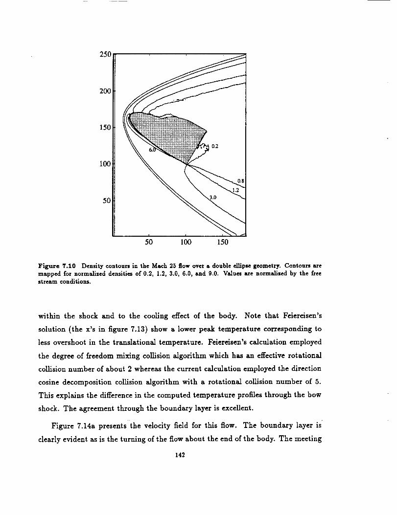
250
200
150
100
50
50 100 150
Figure T.IO Density contours in the Mweh 25 flow over s double ellipse geometry. Contours aremapped for normalized densities of 0.2, 1.2, 3.0, 6.0, and 9.0. Values are normalised by the freestream conditions.
within the shock and to the cooling effect of the body. Note that Feiereisen's
solution (the x's in figure 7.13) show a lower peak temperature corresponding to
less overshoot in the translational temperature. Feiereisen's calculation employed
the degree of freedom mixing collision algoritlma which has an effective rotational
collision number of about 2 whereas the current calculation employed the direction
cosine decomposition collision algorithm with a rotational collision number of 5.
This explains the difference in the computed temperature profiles through the bow
shock. The agreement through the boundary layer is excellent.
Figure 7.14a presents the velocity field for this flow. The boundary layer is
clearly evident as is the turning of the flow about the end of the body. The meeting
142

14
t-
¢a
oz
12
10
6
4
2
X
Distance from Surface (mm)
Figure 7.11 Density along the stagnation streamline. Values are normalized by the free streamconditions. Solid line with 'o' symbols are used for the current results, 'x' symbols are used for thecalculation by Feiereisen (1990).
of the flow over the body with that under the body normally would lead to a wake
shock, however the extremely low densities in the wake for this flow preclude any
evidence of such a shock. It is of interest to investigate more closely the "cusp"
region where the nose and the cowl meet. Figure 7.14b is an expanded view of this
region. The theory predicts a region of reeirculation for such a geometry when the
adverse pressure gradient from the cowl is sufficiently strong to force the boundary
layer to separate. There is no evidence of separation in this figure, although there
definitely is a growth in the boundary layer thickness after the cusp and the region
right at the cusp is virtually stagnant. It is interesting to note from this figure that
there is a small dip velocity at the surface. This is predicted by kinetic theory (cf.
143

250
200
150
100
50
50 100 150
Figure T.12 Temperature contours for Msch 25 flow over s double ellipse geometry. Contours aremapped for normalised temperatures of 1.2, 20, 40, 60, 80, and 100. Values s_e normalized by thefree stream conditions.
Patterson (1956)) when the mean free path is of the same order as the boundary
layer thickness. This slip velocity is due to the flux of particles incident on the
surface. On average, molecules strike the surface with the momentum existing at
one mean free path from the surface. H the mean free path is of the same order as the
scale to which one is resolving the solution, then one expects to see this momentum
in the flow. Therefore, although the diffuse reflection at the surface ensures that
particles leaving the surface have no net momentum, the flux of particles onto the
surface does have momentum which gives rise to a net velocity for the gas at the
for completeness, figure 7.15 presents the velocity
144
profile in the

2000 T
1800
1600
1400
1200
1000
800
600
400
200
0-1.8
!x
Distance from Surface (mm)
Figure T.15 Temperature along the stagnation streamline. Values are given in degrees Kelvin.Solid line with 'o' symbols is used for the current results, 'x' symbols axe used for the calculations
by Feiereisen (1990).
stagnation streamline. Again the current results agree quite closely with those
from the Cray 2 implementation. The slight differences which exist are probably
attributable to the different collision algorithms employed. It should be noted
that these Cray 2 calculations are somewhat of an anachronism and the latest
implementation uses the direction cosine decomposition collision algorithm.
In conclusion, the implementation of the Stanford particle simulation method
on the Connection Machine is capable of solving the flow field about a general two
dimensional geometry to a high degree of accuracy. That the solution for the double
ellipse geometry compares favorably with that calculated by the implementation
of this method on the Cray 2 indicates there is consistency between the two
145

220
210
200
50 100 150 2_
(b)
Figure 7.14 Velocity field for Math 25 flow over a double ellipse geometry, a) The complete flowfield, b) The flow field in the vicinity of the cusp where the two eUipses meet.
146

1.2
8
oZ
1 ........ = =i = = ::= = =i = = _ ; _ :: .................:...................:....................................
i i i i ! x ! !
0.8 _ i i i :: x:: i i
0.6
0.4
0.2
0 , i , , , , ,• .8 -1.6 -1.4 -1.2 -1 -0.8 -0.6 -0.4 -0.2 0
Distance from Surface (ram)
Figure 7.15 Velocity along the stagnation streamline. Values are normalised by the free streamconditions. Solid line with 'o' symbols is used for the current results, 'x' symbols are used for thecalculations by Feiereisen (1990).
implementations. The results presented in the two previous sections serve not only
to validate the current implementation but also the method in general. The next
section will consider in some detail the performance of the Connection Machine
with this method.
7.5 Performance
In Chapter 1 of this thesis the motivation for the research was described through
the question: "What price for parallelism?" The answer to this question is given
in this section. The first step towards answering this question is to consider the
147 _

distribution of computational time within the algorithm. This distribution is as
follows:
1) move -- 14%
2) rank -- 40%
3) re-order _ 26%
4) collisions _ 7%
5) sampling- 13%
Within thls breakdown, the rank and re-order represent two communications
intensive events which have no equivalent in the vectorlzable algorithm yet account
for 66% of the computational time in the data parallel algorithm. This is time
being spent on events which are necessitated by the parallel architecture and are
not directly related to the computation required in a particle simulation. Therefore
one can say quantitatively that the price for parallelism amounts to two thirds of
the cost Of the calculation.
It should be emphasized that this fraction remains constant when the calculation
is scaled clown to 16k or 8k physical processors. Therefore it is reasonable to expect
that in scaling up to a greater number of processors this fraction will continue to
remain constant. The property of scalability is extremely important in evaluating
parallel architectures. In many of the MIMD architectures one often finds a less
than linear speed up with increasing number of processors because the fraction of
time spent on communication increases in going to more processors. That the cost
of communication in the particle simulation is scaling linearly on the Connection
Machine is a good indication that on future machines with more processors the
performance of the simulation will improve linearly.
It is of interest also to see how the performance of the simulation scales with
the number of virtual processors. Figure 7.16 presents the computational time as a
function of virtual processor (VP) ratio. The values are normalized by the time at
a VP ratio of 8, the lowest for which measurements were reasonable with the double
ellipse problem of the previous section. Since the VP ratio is directly proportional
to the number of particles in the simulation, one would expect the time to increase
linearly with the VP ratio. The dashed line in the figure is an extrapolation of the
148

i
s-_ 5¢.0
*.J
4
L_
.Nm
3
0Z
2
10
• IJ'JJ" !
s • o i
....................... i........................_....................... i..........2": ...... _........................i........................i......................
** _ s I : : :
iiii .... iiiiiiii10 20 30 40 50 60 70
Virtual Processor Ratio
Figure 7.16 Performance of the simulation as a function of virtual processor (VP) ratio. Thedashed line gives the linear extrapolation of performance at VP ratios of 8 and 16. The actual
performance is better than predicted by linear extrapolation because of the inefficiencies associatedwith lower VP ratios.
computational time based on the slope between the points for a VP ratio of 8 and a
VP ratio of 16. This dashed line emphasizes that most efilcient use of the machine
is made at the higher VP ratios for the reasons outlined in Chapter 2.
In order to determine if the 66% paid for parallelism is too steep a price, it
is necessary to benchmark the performance of the simulation on the Connection
Machine. The code used to generate the results of the previous section was written
fully in C/Paris and run on the 32k processor Connection Machine Model 2 at the
NASA Ames Research Center. The front end used to run this simulation was a
DEC Vax 8800. The simulation employed 2048k virtual processors with a total of
256 MB of memory to simulate up to 2.0 x 10⁶ particles in the flow and a further 105
149

particles in the reservoir. To compare the performance of this implementation with
that of a similar implementation on a different supercomputer it is useful to define a
normalized time for the calculation given as the average time to advance one particle
through one time step. Excluding the reservoir particles, for the calculation of the
double ellipse that value is 2.0psec/particle/timestep. The same calculation fully
vectorized on a single processor of the NA$ Cray 2 took 1.Tpsec/particle/timestep.
It should be noted that the Cray 2 calculation was three dimensional even though
the double ellipse geometry is two dimensional. Nonetheless, it is apparent from
this result that the 66_ price of parallelism is being paid off through the great
computational speed of the Connection Machine.
The final evaluation which needs to be made in judging the Connection Machine
concerns the human effort required to program it. The discussion in section 2.1
on data parallel versus vectorizable algorithms is a good basis for this evaluation.
Because the requirements for a data parallel algorithm are stricter than for a
vectorizable algorithm, programming the Connection Machine is inherently more
difficult than programming a vector computer. The current situation is probably
worse than is implied by this statement because data parallel programming is
relatively new and many of the algorithms which have been fully explored in
vectorizable form have yet to be considered for data parallel form. Therefore one can
expect that as a tradition of data parallel programming evolves there will develop
a greater "intuition" for data parallel algorithms and many of the tasks which now
are new and require some effort to conceptualize in data parallel form will have
become routine and part of the data parallel diction.
Beyond the straight algorithmic considerations there is the question of how
detailed a knowledge of the machine is required for efficient programming. From
the discussion in section 2.4 and most of chapters 4 and 5 it should be abundantly
evident that the promise of "general" communication is a myth for the Connection
Machine. Although one can classify all communication which makes explicit use of
the router as "general", it is incorrect to assume that all such communication comes
at the same price. It is very difficult to make educated guesses at the particular
cost for any communications event in a proposed algorithm; for the most part
150

all variations in an algorithm have to be implemented before an optimum can be
selected. There is no well defined hierarchy of memory as exists in conventional
computers because memory access times through the communications network are
dependent on a large number of variables. Through experience it is possible to gain
some intuition for the performance of communications but this certainly requires an
effort which is unnecessary in programming conventional or even vector computers.
Again part of the problem may be attributed to the infancy of this technology and
in the future much of this effort may be unnecessary as the technology matures and
languages and compilers for this architecture improve.
r-
151


Chapter 8
Multiple Species and Chemistry
The work presented thus far has resulted in a particle simulation capable of
simulating a single specie diatomic gas in hypersonic flow with no chemical reactions.
This is the foundation upon which algorithms for simulating multiple species with
chemical reactions can be built. This chapter outlines how these algorithms may
best be implemented on the Connection Machine and identifies possible problems
one may encounter in carrying out such work. It should be emphasized that none of
the algorithms described in this chapter have been implemented on the Connection
Machine and the purpose of this chapter is only to serve as a guide in this area.
8.1 Reaction Fundamentals
Atmospheric air subjected to hypersonic conditions can be modelled as a
five species set composed of O2, N2, NO, O, and N. There are 15 dissoci-
ation/recombination reactions and 4 exchange reactions associated with this set
(Moss and Bird (1985)). In addition there are 15 allowable collision classes where a
collision class is defined by any combination of two species. The collision selection
rule for multiple species must account for the different number densities and the
different sample sizes for each collision class within a given cell. Once a collision has
152"

beendecided upon the colliding pair must be tested to see if it will undergo reaction.
Each reaction is characterized macroscopically with a reaction rate coefficient,
kf(T), and a species concentration coefficient, K(T), as fit by experiment. In a
particle simulation, a distinct selection rule must be implemented for each reaction
in order to reproduce the macroscopic reaction rate temperature-dependence. Pairs
of particles which do not react undergo a regular thermal coUision.
Dissociation reactions are characterized by the general equation
AB + X ---. A + B + X (8.1)
where AB is a diatomic molecule, A and B are monatomic particles, and X is a
partner of any type. Only collisions with collision energy exceeding the threshold
dissociation energy, E d, are allowed to dissociate. Dissociation reactions are
endothermic and the energy removed from the reactants would, in a real collision, be
redistributed in the electron configuration of the products. In a particle simulation
the electronic state of a particle is not usually modelled since it does not contribute
energy in a collision. Consequently the dissociation energy must be removed from
the system. Note, however, that the reverse reaction is exothermic therefore, at
equilibrium, this energy is returned to the system at the same rate it is removed.
Exchange reactions are characterized by the general equation
AB + C AC + B (8.2)
where (7 is a monatomic particle. This reaction also requires the splitting of
a molecule and therefore can only proceed if the collision energy exceeds the
dissociation energy. However the reaction also results in the creation of a new
diatomic molecule which allows the release of energy Ed,,,. That is, the dissociation
energy for the revers e reaction must be returned to the system. Therefore the
reaction requires energy AE = E,/- Ed,,, to be removed from the reactants and
redistributed as potential energy in the products.
Recombination is the reverse of dissociation; it is inherently a three-body
process but can be modelled by two successive binary collisions. The first collision
153

requires two colliding atoms to form an unstable union characterized as a mutually
orbiting pair. Therefore,
A + B _ (AB) (8.3)
where (AB) is the orbital pair formed from atoms A and B. Orbiting pairs have a
limited lifetime dependent upon the collision energy. If an orbital pair undergoes
a collision within its lifetime it may then stabilize into a molecule thus completing
the recombination process. This process is modelled by the equation
(AB) + X _ AB + X (8.4).
The dissociation energy, Ed, removed from the reactants in (8.1) must now be
returned to the products of (8.4). If no stabilizing collision occurs during an orbital
pair's lifetime then the pair is split into its free atoms.
8.2 Implementing Multiple Species
The first step towards chemical modelling in the simulation is to introduce
the capability for simulating multiple species. The different species which may be
encountered in simulating the flow of a gas may be broadly classified into three
categories: monatomic particles, dlatomic molecules, and orbital pairs. The last of
these three is only encountered when modelling recombination reactions and will be
discussed more fully in the section on chemistry. This section concerns itself only
with the implementation of multiple species without chemical reactions.
The introduction of multiple species necessitates the specification of additional
information concerning the different species. The actual number of species which
are usually modelled is relatively small; hypersonic flows involving air are commonly
modelled with a total of 5 different species, although the inclusion of recombination
reactions requires an additional three species for the orbital pairs. This information
is best stored in the front end computer, and the Connection Machine processors
154

representing the particles need only store a pointer to the appropriate table entry.
The broadcast of information from the front end to the individual processors is
very fast in comparison to either NEWS or general router communication. For
the processors to get the species information from the front end it is necessary
only to identify the processors representing particles of each species and copy the
appropriate front end information into the processors. Information pertaining to a
collision class may be stored in the same fashion. For the 8 species model there are 36
possible collision classes. This number is still small enough to make broadcasting
from the front end a viable communications alternative for information which is
strictly dependent only on the collision class. A problem arises when the necessary
information is dependent not only on the collision class but also on the cell in the
simulation, as with the determination of the collision class sample size discussed
below.
If there is to be no chemical reaction the only additional information necessary
for the calculation is the species mass and the collision cross section. The cross
section is necessary in evaluating the probability of selection, Pj, for the candidate
pairs. With multiple species, the probability of selection for collision of a particular
candidate pair of particles, the first of specie a and the second of specie b, is given
by (McDonald 1990)
nanb _ -2 _..A_ .
P" = (1 (8.5)
where na and n b are the number densities for specie a and specie b respectively, $ab
is the Kronecker delta, Sab is the sample size of candidate pairs in class ab, fld2 b
is the hard sphere collision cross section, g is the relative speed, nab is the power
defining the power-law interaction potential, and At is the time step.
The greatest difficulty one encounters when evaluating this expression is in
determining the values of ha, n b and Sab. For the single specie case, the sample
size is always n/2 and determining n requires two scan instructions, that is,
a CH_enumerate followed by a CH_scan_with_copy. The most straightforward
approach for multiple species is to extend this directly, then for an 8 species model
155

one would require 16 scan instructions to determine the values of na and n b and an
additional 70 scan instructions to determine the value of ,.,Cab. Note that these 70
scans would be across candidate pairs and could be carried out at half the VP ratio of
the particles' VP set by using VP alia.sing. Therefore they would be approximately
equivMent to 35 scans at the higher VP ratio.
In practice a large fraction of all the coUisions will fall into one of five classes.
Specifically the three classes involving O2 and N 2 are most common in the free
stream and the two additional classes involving O and N2 are most common after
the shock where most of the O2 molecules have dissociated. Therefore the 70
scan instructions necessary for determining Sab may not be overly expensive since
many of the collision classes are sparsely populated and hardware contention in the
communications would be reduced. This sparsity may be used to some advantage
in reducing the communications by employing a different algorithm for determining
the sample sizes in the less common coUision classes. In such an approach one
first determines the sample sizes associated with the five most common coUision
classes by using the necessary scan instructions. Then to get the sample sizes for
the remaining classes one employs a multi-grid algorithm similar to that described
in Chapter 4. One creates a multi-grid with elements for each ceU in the simulation
and with a level for each remaining collision class. Therefore each remaining collision
class is mapped to a level of the multi-grid and each ceU in the simulation is mapped
to an element in a level of the multi-grid. One processor from each candidate
coUision pair then uses the CM_send_with_add instruction to send a value of 1 to the
appropriate grid element in its 1eve1. This results in each element in a particular
level of the multi-grid storing the sample size for the collision class associated
with that level. The same processor in the candidate pair then uses the CM_get
instruction to get this value from the multi-grid. This algorithm takes advantage of
the fact that the performance of general communication can improve dramatically
with a reduction in router contention. Therefore this approach is suitable if it can
be determined that over the whole flow field certain coUision classes are greatly
dominant leaving the remaining collision classes relatively sparse.
With the various factors comprising (8.5) made available, the probability of
156

selection is evaluated and the decision to collide a candidate pair is made. If there is
no chemical reaction, then the next step is to carry out the appropriate collision me-
chanics. The introduction of three classes of particles necessitates the specification
of three types of collision, specificany monatomic-monatomic, monatomic-diatomic,
and diatomic-diatomic. Note that orbital pairs do not undergo collision as such and
must either split into separate atoms or stabilize into diatomic molecules before
undergoing coUision. The mechaaics of each of these three types of collisions are
identical to those already implemented. The diatomic-diatomic collision mechanics
are covered in Chapter 3; the monatomic-monatomic and the monatomic-diatomic
collision mechanics correspond to the diatomic-diatomic collision mechanics with no
exchange of internal energy. Therefore the introduction of multiple species does not
require the specification of new collision mechanics; the conision mechanics already
specified for the single specie diatomic particle simulation can be employed with
only the introduction of the appropriate switch for the different particle classes.
8.3 Implementing Chemical Reactions
The addition of chemical reactions amongst the multiple species introduces
no new communications problems. Once the decision to coUide a pair has been
made, the information necessary to decide on a reaction is strictly dependent on
the species involved in the coUision. This information can be stored in the front
end and accessed very efficiently as described in the previous section. This is one
of the few situations in the particle simulation algorithm where the amount of
arithmetic computation is likely to exceed the communications. The probabilities
which must be computed for deciding on a reaction are given by complicated
expressions involving several transcendental functions potentially making this is
an ideal situation for the Connection Machine since it allows its floating point
performance to be put to full use.
8.3.1 Reaction Mechanics
The three types of reactions, dissociation, exchange, and recombination, were
157

described in the first section of this chapter. Figure (8.1) presents a flow chart for
the collision process when these reactions are included (Haas (1990)). Note that
recombination is modelled by a two step process therefore there are two branches
in the flow chart for recombination. The mechanics associated with reactions are
carried out only after a candidate pair has been accepted for collision. The selection
rule for accepting candidate pairs has to be modified as described in the previous
section to allow for multiple species.
Reaction types are identified on the basis of the participating particles.
Dissociation reactions are allowed with all collisions of two diatomic particles or with
half the collisions involving a diatomic and a monatomic particle. The other half of
the collisions involving a diatomic and a monatondc particle may lead to exchange
reactions. Collisions involving an orbital pair may lead to recombination reactions
and collisions involving two monatomic particles always lead to the formation of an
orbital pair, the first step in a recombination reaction. The calculation associated
with each of these reactions must be carried out independently.
Dissociation reactions are allowed to occur with probability Pd given by (Haas
(1990))
]
Pd= P0(1- _ 1)P (8.6)
where e is the ratio of the collision energy to the dissociation energy, and P0, PI and
P2 are constants dependent on the species. The collision energy must be known
in all collisions and is calculated for all colliding pairs. The reaction constants
are stored in the front end and broadcast to the processors. This probability is
evaluated for all collisions which are allowed to lead to the dissociation of a colliding
particle. The dissociation of a particle requires the creation of a new particle and
the redistribution of the post-reaction energy. The creation and destruction of
particles deserves special attention and the discussion of these processes is given in
the following subsection.
The probability for the occurrence of an exchange reaction is of the same form as
equation (8.6). Exchange reactions neither create nor destroy particles; the outcome
158

CANDIDATE
PAIR
,/
ReactionTypes
1
ReactionSelection
tN. / \/
ReactionMechanics
I
AB + CD
AB +C
ACCEPT
AB
ACCEPT
ACCEPT
REACTION
STABILIZE
(AB)
SPLIT PAIR
(AB)
A+B
:[ FORM PAIR[(AB)
_1 NO- [COLLISION [
Figure 8.1 Flow chart for the collision process with the inclusion of chemical reactions. Four
distinct reaction types axe Mlowed based on the classes of paxtides participating in the collision.
(Haas(1990))
is strictly a redistribution of energy and alteration of species. Exchange reactions
are considered for half the collisions involving a monatomie and a diatomic particle
thus leaving the other half of these types of collision to be considered for dissociative
reactions. The split is made arbitrarily on the basis of the class of the first particle
in the pair. If this particle is diatomic then the pair is considered for a dissociation
reaction whereas if this particle is monatomic then the coRision is considered for an
exchange reaction.
159

The probability Pr for the occurrence of a recombination reaction is given by
(Haas (1900))
e, = (8.7)
where eint, 0 and eint, 1 are the internal energies for the orbital pair and the collision
partner respectively, and P3, P4 and P5 are constants dependent on the species. The
probability given by equation (8.7) is evaluated for all collisions which involve an
orbital pair. If the partner is monatomic then the probability of reaction is based
only on the internal energy of the orbital pair, in other words ein_, 1 is set to unity.
If a collision leads to recombination then the orbital pair involved in the collision
is stabilized to its diatomic equivalent. If recombination does not occur then the
orbital pair is split into two monatomic particles of the species defining the pair.
As with dissociation reactions, this requires the creation of a new particle. For
reasons of efficiency it is best to create all new particles at the same time, therefore
new particles resulting from split orbital pairs are created at the same time as new
particles resulting from the dissociation of diatomic particles.
Any collisions involving two monatomic particles always lead to the creation of
an orbital pair and the corresponding destruction of a particle. The creation of an
orbital pair is the first step in a recombination reaction therefore it is not, strictly
speaking, a fourth type of reaction. However, for the modelling of chemistry in a
particle simulation it is convenient to view this process as a distinct reaction since
it must be carried out separately from the other three processes.
8.3.2 Creation and Destruction of Particles
New particles are created from dissociation reactions and from failed recombi-
nation reactions. Particles for this purpose are available from the reservoir. Once
all the reactions leading to the creation of a new particle have been identified, they
are enumerated and the enumeration is used as an index into the reservoir. The
appropriate state information is then sent to these reservoir particles to change
them to their new state.
160

The creation of particles in this manner leaves the system of particles in a
disordered state at the end of the time step. Consequently the merged ordered
subsets sorting algorithm must be revised to allow for this situation. Since the new
particles are, amongst themselves, in an ordered state, the sorting algorithm need
be revised only to include the merging of an additional ordered system.
The destruction of particles involves the same process as the removal of particles
which exit downstream of the simulation. These particles are simply converted
to reservoir particles by changing their physical state and setting their ceU index
to point to the reservoir. Since t_s process is identical to the removal of exited
particles, it proves most efficient to perform the two processes at the same time.
8.3.3 Estimated Cost
There are no apparent difficulties in extending the current implementation to
include multiple species and chemistry. The greatest foreseeable cost wiU be in
applying equation (8.5) to select pairs for collision. The straightforward application
of (8.5) requires the equivalent of 51 scan instructions at the VP ratio of the
particles' VP set. Since scans are about an order of magnitude faster than sends,
the associated communications cost would be approximately equivalent to 5 send
instructions. Therefore the amount of communications wiU probably be about
equivalent to that associated with re-ordering the particle data, which currently
takes 26% of the computational time (section 7.5). This, of course, is a very
approximate estimate. The cost for the arithmetic computation is equally difficult
to estimate but certainly wiU not exceed the cost of communication. Therefore
a very conservative estimate on the total additional cost for simulating multiple
species with chemistry is another 50% of the computational time.
161

Chapter 9
Concluding Remarks
9.1 Summary
Currently the fluid mechanics community is seeing a resurgence of interest in
rarefied gas dynamics, a regime where computational methods often offer the only
viable means of solving flow problems of practical interest. The method of direct
particle simulation is one of the few methods, suitable to this regime, which provides
accurate solutions at reasonable computational cost. Nonetheless, the expense
associated with this method is such that solutions to engineering problems almost
exclusively require the use of a supercomputer. The Stanford particle simulation
(SPS) method has been developed to make the most efficient use of supercomputer
architectures thereby allowing broader application of the direct particle simulation
method.
It is largely accepted that future improvements in supercomputing performance
will be in the direction of increased parallelism, and massively parallel architectures
represent the research frontier in this direction. The massively parallel architecture
of the Connection Machine has been successfully applied to a wide variety of
scientific problems. The purpose of the current work has been to investigate the
162

suitability of this architecture, and this machine in particular, for the direct particle
simulation of rarefied gas dynamic flows.
The work progressed in three stages. The first stage required the development
of data parallel algorithms for particle simulation. Some of these algorithms
were directly translatable from their vectorizable form, and these are described
in Chapter 3. However several of the vectorizable algorithms could not be readily
extended to data parallel form. These required new algorithms to be developed, and
in particular, the sorting algorithms of Chapter 4 were an outcome of this effort.
The second stage involved optimizing the implemented algorithms to the Con-
nection Machine architecture. This work required an intimate understanding of the
communications network and resulted in the development of new communications
algorithms. The master/slave algorithm of Chapter 5 was an important result of
this effort. A related algorithm also is applied to the sampling of macroscopic flow
quantities from the simulation and is described in section 3.4.
The third and final stage of the work required validating the implementation
and gauging its performance. A large number of test calculations were performed
and Chapter 7 presents the pertinent results. Thermal relaxation histories and the
shock wave profiles are standard test calculations used to validate computational
methods for rarefied gas dynamics. The reflected shock problem goes significantly
further as a validation both of the implementation and the method. The results from
that calculation also _ghlight some of the di_culties and inadequacies associated
with direct particle simulation, especially as the continuum limit is approached. As
further validation, the flow over a double ellipse was calculated and the results were
compared to those from the implementation of the SPS method on the Cray 2. This
calculation was also used to gauge the performance of the Connection Machine for
direct particle simulation, and this is discussed in some detail in section 7.5.
9.2 Conclusions
An important result of this investigation has been a quantitative measure of
163

the performance of the Connection Machine for direct particle simulation. From
this result it has been possible to conclude that the massively parallel architecture
of the Connection Machine is quite suitable for this type of calculation. However,
there are difilculties in taking full advantage of this architecture because of the lack
of a broad based tradition of data paraUel programming. An important outcome of
this work has been new data parallel algorithms specifically of use for direct particle
simulation but which also expand the data parallel diction.
r,
164


References
ALDOUS, D. and DIACONIS, P., American Mathematical Monthly, 93,333,
(1986).
ALSMEYER, H., Journal of Fluid Mechanics, 74, 497, (1976).
BAGANOFF, D., Journal of Fluid Mechanics, 23, 209, (1965).
BAGANOFF, D., Simulation of Gas Motion by a Collection of ParticleJ, Proceed-
ings of the IBM ACIS University Conference, Boston, Vol. II, p.304, (1987).
BAGANOFF, D. and MCDONALD, 3.D., A ColliJion-Selection Rule for a Particle
Simulation Method Suited to Vector ComputerJ, To appear in Physics of Fluids
A, (July 1990).
BIRD, G.A., Physics of Fluids, 6, 1518, (1963).
BIRD, G.A., Physics of Fluids, 13, 1172, (1970).
BIRD, G.A., Molecular Gas Dynamics, Clarendon Press, Oxford, (1976).
BIRD, G.A., Monte-Carlo Simulation in an Engineering Contezt, Invited paper
221, International Symposium on Rarefied Gas Dynamics, Charlottesville, Va.,
(1980).
BIRD, G.A., Physics of Fluids, 26, 3222, (1983).
165

BIRD, G.A., Perception of Numerical Methods in Rarefied Gasdynamics, Invited
paper, 16 th International Symposium on Rarefied Gas Dynamics, Pasadena, Ca.,
(1989).
BORGNAKKE, C. and LARSEN, P.S., Journal of Computational Physics, 18, 405,
(1975).
BOYD, I.D., Direct Simulation o/Rotational and Vibrational Nonequilibrium,
AIAA-89-1880, (1989).
BOYD, I.D., Vectorization of a Monte Carlo Scheme, Submitted to Journal of
Computational Physics, (1990).
BURNETT, D., Proceedings of the London Mathematical Society, 39, 382,
(1935).
?
DAVIS, J., DOMINY, R.G., HARVEY, J.K. and MACROSSAN, M.N., Journal of
Fluid Mechanics, 135,355, (1983).
FEIEREISEN, W.J. and MCDONALD, J.D., Three DimenJionaI Discrete Particle
Simulation o/an AOTV, AIAA-89--1711, (1989).
FEIEREISEN, W.J., An Assessment o/ "Shuffle Algorithm" Collision Mechanics
for Particle Simulation, 17 th International Symposium on Rarefied Gas Dynam-
ics, Aachen, Germany, (1990).
FEIEREISEN, W.J., The Hypersonic Double Ellipse in Rarefied Flow, INRIA
Workshop on Hypersonic Flows for Reentry Problems, Antibes, France, (1990).
FISCKO, K. A., Ph.D. Thesis, Dept. of Aeronautics and Astronautics, Stanford
University, (1989).
FLYNN, M.J., IEEE Trans. Computers, C-21 9, 948, (1972).
GOODMAN, F.O. and WACHMAN, H.Y., Dynamics of Gas-Surface Scattering,
Academic Press, (1976).
GUTTMAN, I., WlLKS, S.S. and HUNTER, J.S., Introductory Engineering
Statistics, :John Wiley and Sons, Inc., Toronto, (1971).
HAAS, B.L., Fundamentals of Chemistry Modelling Applicable to a Vectorized
Particle Simulation, AIAA-90-1749, (1990).
166

HANSEN, C.F., Rate Processes in Gas Phase, NASA Reference Publication 1090,
(1983).
HANSON, R.K., AIAA Journal, 9, 1811, (1971).
HILLIS, W.D. and STEELE, G.L., Communications of the ACM, 29, 1170,
(1986).
HINSHELWOOD, C.N., The Kinetics of Chemical Change , Clarendon Press,
Oxford, (1940).
HURLBUT, F.C., Gas/Surface Scatter Models for Satellite Applications, AIAA
Progress in Aeronautics and Astronautics, Vol. 103, pp. 98-119, (1986).
KNUTH, D.E., The Art of Computer Programming; Volume _: Seminurnerical
Algorithms, Addison Wesley Publishing Company, (1973).
LORDI, J.A. and MATES, R.E., Physics of Fluids, 13, 291, (1970).
LUMPKIN, F.E., Ph.D. Thesis, Dept. of Aeronautics and Astronautics, Stanford
University, (1990).
LUMPKIN, F.E., CHAPMAN, D.R. and PARK, C., A New Rotational ReIazation
Model for Use In Hypersonic Computational Fluid Mechanics, AIAA-89-1737,
(1989).
MCDONALD, J.D. and BAGANOFF, D., Vectorization of a Particle Simulation
Method for Hypersonic Rarefied Flow, AIAA-88-2735, (1988).
MCDONALD, J.D., Ph.D. Thesis, Dept. of Aeronautics and Astronautics,
Stanford University, (1990).
MELVILLE, W.K., Journal of Fluid Mechanics, 51,571, (1972).
Moss, J.N. and BIRD, G.A., Direct Simulation of Transitional Flow for Hyper-
sonic Reentry Conditions, AIAA Progress in Aeronautics and Astronautics, Vol.
96, pp. 113-139, (1985).
MYERS, D.W. and ADAMS, G.B., Benchmarking and Performance Analysis
of the CM-I_, Proceedings of the Conference on Scientific Applications of the
Connection Machine, Moffet Field, Ca., (1988).
167

NANBU, K., Journal of the Physical Society of Japan, 49, 2042, (1980).
PARKER, C., Physics of Fluids, 2, 449, (1959).
PATTERSON, G.N., Molecular Flow of Gases, John Wiley and Sons, Inc., New
York, (1956).
PLOSS, H., Computing, 38, 101, (1987).
PRYOR, D.V. and BURNS, P.J, Vectorized Monte Carlo Molecular Aerodynamics
Simulation of the Rayleigh Problem, Proceedings of Supercomputing '88, Or-
lando, pp. 384-391, (1988).
PULLIN, D.I., Physics of Fluids, 21,209, (1978).
THINKING MACHINES CORP., The Connection Machine System, Paris Release
Notes, Thinking Machines Corp., (1989).
VINCENTI, W.G. and KRUGER, C.H., Introduction to Physical Gas Dynamics,
John Wiley and Sons, Inc., New York, (1965).
WENAAS, E.P., Journal of Chemical Physics, 54, 376, (1971).
WORONOWICZ, M.S. and McDONALD, J.D., Application of a Vectorized Particle
Simulation in High-Speed Near-Continuum Flow, AIAA-89-1665, (1989).
168