ON THE STABILIZATION OF THE BRESSE BEAM WITH KELVIN …

HAL Id: hal-02070211https://hal.archives-ouvertes.fr/hal-02070211

Preprint submitted on 16 Mar 2019

HAL is a multi-disciplinary open accessarchive for the deposit and dissemination of sci-entific research documents, whether they are pub-lished or not. The documents may come fromteaching and research institutions in France orabroad, or from public or private research centers.

L’archive ouverte pluridisciplinaire HAL, estdestinée au dépôt et à la diffusion de documentsscientifiques de niveau recherche, publiés ou non,émanant des établissements d’enseignement et derecherche français ou étrangers, des laboratoirespublics ou privés.

ON THE STABILIZATION OF THE BRESSE BEAMWITH KELVIN-VOIGHT DAMPING

Toufic El Arwadi, Wael Youssef

To cite this version:Toufic El Arwadi, Wael Youssef. ON THE STABILIZATION OF THE BRESSE BEAM WITHKELVIN-VOIGHT DAMPING. 2019. hal-02070211

https://hal.archives-ouvertes.fr/hal-02070211

https://hal.archives-ouvertes.fr

ON THE STABILIZATION OF THE BRESSE BEAM WITHKELVIN-VOIGHT DAMPING

TOUFIC EL ARWADI AND WAEL YOUSSEF

Abstract. The aim of this paper is to study the theoretical and numericalstability of the Bresse system in one-dimensional bounded domain with vis-coelastic Kelvin-Voigt damping. We first showed the well posedness of thesystem . Then the stability is obtained by applying The multiplier techniques. Later a numerical scheme is proposed and analyzed. Finally a priori errorestimate is established.

1. Introduction

Some of the properties of viscoelastic materials are their ability to creep, re-cover, undergo stress relaxation and absorb energy. Owing to huge applications ofsmart materials in modern technology, there has been an abundance of literatureon the study of elastic systems with viscoelastic damping. When a smart materialis patched in an elastic structure, the Young’s modulus, the mass density and thedamping coefficients are changed accordingly. Practically, one type of viscoelasticdamping is usually used. This is the Kelvin-Voigt damping. This kind of damp-ing, on the one hand, make the distributed control practically realizable, and onthe other hand, bring some new mathematical challenges that attract increasingresearch interests.In this work, the theoretical and numerical stability of a viscoelastic Bresse systemis investigated. The Bresse system is also known as the circular arch problem andis given by the following equations:

(1.1)ρ1φtt = Qx + IN + F1,ρ2ψtt =Mx −Q+ F2,ρ1wtt = Nx − IQ+ F3,

whereN = κ0(wx − lφ), Q = κ(φx + lw + ψ), M = bψx.

We use N, Q and M to denote the axial force, the shear force and the bendingmoment. ω, φ and ψ denote the longitudinal, vertical and shear angle displace-ments, respectively. Furthermore, ρ1 = ρA, ρ2 = ρI, k0 = EA, k = k′GA, b = EIand l = R−1, where ρ denotes the density, E is the elastic modulus, G is the shearmodulus, k′ is the shear factor, A is the cross-sectional area, I is the second momentof area of the cross-section and R is the radius of curvature of the beam. Here,we assume that all the above coefficients are positive constants. Finally, Fi denote

Date: March 16, 2019.Key words and phrases. Bresse beam; Kelvin-Voight damping; finite element discretization.

1

2 TOUFIC EL ARWADI AND WAEL YOUSSEF

external forces. Therefore, without external forces, the motion equations are givenby

ρ1φtt − κ(φx + ψ + lω)x − κ0l(ωx − lφ) = 0 in (0, L)× (0,∞),(1.2)ρ2ψtt − bψxx + κ(φx + ψ + lω) = 0 in (0, L)× (0,∞),(1.3)

ρ1ωtt − κ0(ωx − lφ)x + κl(φx + ψ + lω) = 0 in (0, L)× (0,∞),(1.4)

b

b

L

ψ

ω

φ

M0

M

Figure: After deformation the particle M0 of the beam take the position M

Considering Bresse equations with Kelvin-Voigt damping, the external forces aregiven by:

(1.5)

F1 = γ1(φx + lw + ψ)xt + γ0l(wx − lφ)t,F2 = γ2ψxxt + γ1(φx + lw + ψ)t,F3 = γ0(ωx − lφ)xt − γ1l(φx + ψ + lω)t,

where γ1, γ2 and γ2 are the damping coefficients. Hence, by substituting Fi in (1.1)we get our desired viscoelastic Bresse type system

(1.6)

ρ1φtt − k(φx + lω + ψ)x − γ1(φx + lw + ψ)xt − k0l(ωx − lφ)−γ0l(wx − lφ)t = 0 in (0, L)× (0,∞),

ρ2ψtt − bψxx − γ2ψxxt + k(φx + ψ + lω)+γ1(φx + lω + ψ)t = 0 in (0, L)× (0,∞),

ρ1ωtt − k0(ωx − lφ)x − γ0(ωx − lφ)xt + kl(φx + ψ + lω)+γ1l(φx + ψ + lω)t = 0 in (0, L)× (0,∞).

with t > 0 and 0 < x < L, where L represents the distance between the ends of thecenter line of the beam, see figure.One type of boundary conditions is considered:Dirichlet-Dirichlet-Dirichlet

(1.7) φ(t, x) = ψ(t, x) = ω(t, x) = 0, x = 0, L.

3

The initial conditions for this system are given by:

(1.8) ω(0, .) = ω0, ωt(0, .) = ω1, φ(0, .) = φ0, φt(0, .) = φ1,ψ(0, .) = ψ0, ψt(0, .) = ψ1 on (0, L).

The energy of solutions of the system (1.6) is defined by

(1.9)

E(t) = 1

2

∫ L

0

(ρ1|φt|2 + ρ2|ψt|2 + ρ1|ωt|2 + b|ψx|2

+k|φx + ψ + lω|2 + k0|ωx − lφ|2)dx.

So, the dissipation relation is given by

(1.10)d

dtE(t) = −

∫ L

0

(γ2|ψxt|2 + γ1|φx + ψ + lω|2 + γ0|ωxt − lφt|2

)dx.

Many authors treated the stability of beams under the influence of controls andfeedbacks with viscoelastic terms. In [23] S. Chen and al. studied the mathemati-cal properties of a variational second order evolution equation. As an application,they considered the Euler-Bernoulli and Rayleigh beams with the global or localKelvin-Voigt damping. They establish the strong asymptotic stability and expo-nential stability. Later, K. Liu and Z. Liu [24] studied the energy decay rate for anone-dimensional linear wave equation with the Kelvin-Voigt damping presented ona subinterval which models an elastic string with one segment made of viscoelasticmaterial and the other of elastic material. It was proved that the energy of thatsystem does not decay exponentially when each segment is homogeneous, i.e., co-efficient functions are piecewise constant and have discontinuity at the interface.In [28] Tatar prove an exponential decay of solutions of viscoelastic Timoshenkobeam for a large class of kernels with weak conditions. We refer also to A. Guesmiaand S. A. Massaoudi [12] which established an exponential and polynomial decayresults for the Timoshenko system with a viscoelastic damping. The same authorsshowed in [13] a general stability estimate using the multiplier method and someproperties of convex functions. Also, we refer the reader for some other results onthe Bresse system [1, 3, 10, 11, 15, 18, 25, 26, 29, 30].On the other hand, we mention some numerical studies for some beam models.Copetti and Fernaández [6] considered a dynamic contact problem between a vis-coelastic beam and a deformable obstacle. They introduced a fully discrete approx-imations, based on the finite element method to approximate the spatial variableand the implicit Euler scheme to discretize the time derivatives. Moreover, thyeproved a priori error estimates, obtaining the linear convergence of the algorithmunder an additional regularity condition. In [4] Bernardi and Copetti considereda nonlinear model for a thermoviscoelastic Timoshenko beam that can enter incontact with obstacles and they performed the a priori analysis of the discreteproblem by proposing a discretization by combining an Euler and Crank-Nicolsontype schemes in time and finite elements in space. In [2] Ahn and Stewart con-sidered of a viscoelastic (Kelvin-Voigt type) Timoshenko beam. The existence ofsolutions is proved using the conservation of energy, which is performed both the-oretically and numerically.

The remaining work of this paper is organized as follows. In section 2. thesystems (1.6), (1.7), (1.8) and (1.6), (??), (1.8) are formulated in an appropriateHilbert state spaces setting and the well posedness of the systems is proved. In sec-tion 3, the exponential decay rate of each of the system is showed. In section 4, a


numerical scheme based on the finite element method is introduced to approximatethe solution. In addition, the decay of the discrete energy is obtained.

2. Well-posedness

In this section, we shall study the existence and uniqueness of the solution of theviscoelastic Bresse system (1.6) corresponding to the boundary conditions (1.7) andthe initial conditions (1.8) by means the semigroup theory. To attend the differenttypes of boundary conditions, we consider the following product Hilbert spaces:

H = H10 (0, L)× L2(0, L)×H1

0 (0, L)× L2(0, L)×H10 (0, L)× L2(0, L).

The space H is equipped with the inner product which induces the energy norm(2.11)∥U∥2H = ∥(φ,Φ, ψ,Ψ, ω,W )∥2Hj

= ρ1∥Ψ∥2 + ρ2∥Ψ∥2 + ρ1∥W∥2 + κ∥φx + ψ + lω∥2 + b∥ψx∥2 + κ0∥ωx − lφ∥2.

Here and after, ∥·∥ denotes the L2(0, L) norm. We rewrite the initial-value problem(1.6), (1.7), (1.8) as a first-order system for U = (φ,Φ, ψ,Ψ, ω,W ) on the Hilbertspace H as follows:

(2.12) Ut = A U, U(0) = U0.

Let U = (φ,Φ, ψ,Ψ, ω,W ), and we define the linear unbounded operators A =A+ B : D(A ) → H by

(2.13) A =

0 1 0 0 0 0κρ1D2 − κ0l

2

ρ1I 0 κ

ρ1D 0 (κ+κ0)l

ρ1D 0

0 0 0 1 0 0− κ

ρ2D 0 b

ρ2D2 − κ

ρ2I 0 −κl

ρ2I 0

0 0 0 0 0 1

− (κ+κ0)lρ1

D 0 − κlρ1I 0 κ0

ρ1D2 − κl2

ρ1I 0

,

(2.14) B =

0 1 0 0 0 0

0 γ1

ρ1D2 − γ0l

2

ρ1I 0 γ1

ρ1D 0 (γ1+γ0)l

ρ1D

0 0 0 1 0 0

0 −γ1

ρ2D 0 γ2

ρ2D2 − γ1

ρ2I 0 −γ1l

ρ2I

0 0 0 0 0 1

0 − (γ1+γ0)lρ1

D 0 −γ1lρ1I 0 γ0

ρ1D2 − γ1l

2

ρ1I

,

where Di = di/dxi and(2.15)D(A ) = U ∈ H1 : Φ, Ψ, W ∈ H1

0 (0, L), κ0ω + γ0W ∈ H2(0, L), κφ+ γ1Φ ∈ H2(0, L)

bψ + γ2Ψ ∈ H2(0, L).

Now, the next theorem provides the well-posedness of (1.6),(1.7),(1.8).

Theorem 2.1. A generates a C0 semigroup S(t) of contractions on H .

5

Proof. Firstly, by a direct calculation, we have

(A U,U)H = −γ1∥Φx∥2 − γ2∥Ψx∥2 − γ0∥Wx∥2 − γ0l2∥Φ∥2 − γ1∥Ψ∥2 − γ1l

2∥W∥2

+2(γ1 + γ0)l

∫ L

0

WxΦdx+ 2γ1

∫ L

0

ΦΨxdx− 2γ1l

∫ L

0

WΨdx

= −γ1∥Φx∥2 − γ2∥Ψx∥2 − γ0∥Wx∥2 − γ0l2∥Φ∥2 − γ1∥Ψ∥2 − γ1l

2∥W∥2

−2γ1l

∫ L

0

WΦxdx+ 2γ0l

∫ L

0

WxΦdx− 2γ1

∫ L

0

ΦxΨdx− 2γ1l

∫ L

0

WΨdx

= −γ1

[∥Φx∥2 + ∥Ψ∥2 + l2∥W∥2 + 2γ1l

∫ L

0

ΦxWdx+ 2γ1

∫ L

0

ΦxΨdx+ 2γ1l

∫ L

0

WΨdx

]

−γ2∥Ψx∥2 − γ0

[∥Wx∥2 + l2∥Φ∥2 − 2l

∫ L

0

WxΦdx

].

Note that the expression multiplied by γ1 is equal to ∥Φx + Ψ + lW∥2 and thatmultiplied by γ0 is equal to ∥Wx − lΦ∥2. Thus,

(A U,U)H = −γ1∥Φx +Ψ+ lW∥2 − γ2∥Ψx∥2 − γ0∥Wx − lΦ∥2 ≤ 0.

So the dissipativity of A is proved. It remains to prove that

(2.16) A U = f, ∀f ∈ D(A ),

where f = (f1, f2, ..., f6), has a unique solution U ∈ D(A ). Indeed, the first threeequations in (1.6) give

u = f1, v = f2, and z = f3.

On the other hand, if we consider the bilinear form defined by

B((φ,ψ, ω), (φ), ψ, ω

):=

∫ L

0

[k(φx + ψ + lω)(φx + ψ + lω) + bψxψx + k0(ωx − lφ)(ωx − lφ)

]dx,

and if we use the Lax-Milgram theorem we conclude that there exists a unique(φ,ψ, ω) solution of the fourth, fifth, and sixth equations of (1.6). Hence, 0 ∈ρ(A) and so by the resolvent identity, for small λ > 0 we have R(λ − A ) = H .Consequently, the Lumer-Phillip theorem implies that A generates a C0 semigroupS(t) of contractions on H .

Therefore the well-posedness is summarized in the following theorem.

Theorem 2.2. If U0 = (φ0, ψ0, ω0, φ1, ψ1, ω1) ∈ D(A ), problems (1.6),(1.7),(1.8)and (1.6),(??),(1.8) admits a unique solution U = (φ,ψ, ω, φt, ψt, ωt) such that

U ∈ C([0,+∞);D(Aj)

)∩ C1([0,+∞);H

).

3. Exponential Stabilization

The main goal of this section is to prove the exponential decay of solutions whichsummarized in the following theorem. Our main tool is the result presented in thefollowing lemma used in Haraux [14] and Lagnese [19] (see [17] for the proof):


Lemma 3.1. Let f : R+ → R+ be a non-increasing function and assume that thereexists a constant T > 0 such that

∫ ∞

t

f(s)ds ≤ Tf(t), ∀t ∈ R+.

Then,

f(t) ≤ f(0)e1− t

T , ∀t ≥ T.

Theorem 3.1. There exist two positive constants C1 and η such that the energyof the solution of (1.6),(1.7),(1.8) satisfies

(3.17) E(t) ≤ C1E(0)e−ηt ∀t ≥ 0.

Proof. Several steps are required for the proof of this theorem.

Step 1. Multiply the first equation of (1.6) by φ, the second by ψ, the thirdby ω, and integrate over [S, T ]× [0, L], we obtain:

(3.18)

−∫ T

S

∫ L

0

ρ1|φt|2 + ρ1

∫ L

0

[φtφ

]TS+ k

∫ T

S

∫ L

0

(φx + ψ + lω)φx

+γ1

∫ T

S

∫ L

0

(φx + ψ + lω)tφx − k0l

∫ T

S

∫ L

0

(ωx − lφ)φ

−lγ0∫ T

S

∫ L

0

(wx − lφ)tφ = 0,

(3.19)

−∫ T

S

∫ L

0

ρ2|ψt|2 + ρ2

∫ L

0

[ψtψ

]TS+ b

∫ T

S

∫ T

S

|ψx|2

+k

∫ T

S

∫ L

0

(φx + ψ + lω)ψ + γ1

∫ T

S

∫ L

0

(φx + ψ + lω)tψ

+γ2

∫ T

S

∫ L

0

ψxtψx = 0

and

(3.20)

−∫ T

S

∫ L

0

ρ1|ωt|2 + ρ1

∫ L

0

[ωtω

]TS+ k0

∫ T

S

∫ L

0

(ωx − lφ)ωx

+lk

∫ T

S

∫ L

0

(φx + ψ + lω)ω + lγ1

∫ T

S

∫ L

0

(φx + ψ + lω)ω

+γ0

∫ T

S

∫ L

0

(ωx − lφ)tωx = 0.

7

Step 2. Adding (3.18), (3.19) et (3.20) leads to(3.21)

−∫ T

S

∫ L

0

ρ1|φt|2 −∫ T

S

∫ L

0

ρ2|ψt|2 −∫ T

S

∫ L

0

ρ1|ωt|2 + k

∫ T

S

∫ L

0

| φx + ψ + lω |2

+k0

∫ T

S

∫ L

0

| ωx − lφ |2 +b

∫ T

S

∫ L

0

|ψx|2 + ρ1

∫ L

0

[φtφ

]TS+ ρ2

∫ L

0

[ψtψ

]TS

+ρ1

∫ L

0

[ωtω

]TS+ γ0

∫ T

S

∫ L

0

(wx − lφ)t(wx − lφ) + γ2

∫ T

S

∫ L

0

ψxtψx

+γ1

∫ T

S

∫ L

0

(φx + ψ + lω)t(φx + ψ + lω) = 0.

Thus, from the definition of E we deduce

(3.22)

k

∫ L

0

| φx + ψ + lω |2 +k0

∫ L

0

| ωx − lφ |2 +b

∫ L

0

|ψx|2

= 2E(t)−∫ L

0

ρ1|φt|2 −∫ L

0

ρ2|ψt|2 −∫ L

0

ρ1|ωt|2.

By combining (3.21) and (3.22) we get

(3.23)

2

∫ T

S

E(t)dt = −ρ1∫ L

0

[φtφ

]TS− ρ2

∫ L

0

[ψtψ

]TS− ρ1

∫ L

0

[ωtω

]TS

+γ0

∫ T

S

∫ L

0

(wx − lφ)t(wx − lφ) + γ2

∫ T

S

∫ L

0

ψxtψx

+γ1

∫ T

S

∫ L

0

(φx + ψ + lω)t(φx + ψ + lω)

+2(∫ T

S

∫ L

0

(ρ1|φt|2 + ρ2|ψt|2 + ρ1|ωt|2)dxdt).

Step 3. In this step, we shall estimate the terms of the right member of (3.23).By using the Young inequality and the Poincaré inequality, we deduce

(3.24) −ρ1∫ L

0

[φtφ

]TS≤ cE(S) ∀S ≥ 0,

(3.25) −ρ2∫ L

0

[ψtψ

]TS≤ cE(S) ∀S ≥ 0,

and

(3.26) −ρ1∫ L

0

[ωtω

]TS≤ cE(S) ∀S ≥ 0,

where c is a generic constant depends on ρ1, ρ2, E, I, G, γ0, γ1, and γ2.On the other hand, the Cauchy-Shwarz and the Poincaré inequalities give us∫ T

S

∫ L

0

(wx − lφ)t(wx − lφ) ≤∫ T

S

(∫ L

0

|(wx − lφ)t|2dx) 1

2(∫ L

0

|wx − lφ|2dx) 1

2

dt.


Hence, (1.10) implies∫ T

S

∫ L

0

(wx − lφ)t(wx − lφ) ≤∫ T

S

(−E ′)12 E 1

2

≤ c

ε

∫ T

S

(−E ′)dt+ ε

∫ T

S

Edt,

for all ε > 0 from Young’s inequality. Therefore, we have

(3.27)∫ T

S

∫ L

0

(wx − lφ)t(wx − lφ) ≤ cE(S) + 1

2

∫ T

S

Edt ∀S ≥ 0.

By repeating the same argument to∫ T

S

∫ L

0

ψxtψx

and ∫ T

S

∫ L

0

(φx + ψ + lω)t(φx + ψ + lω),

we conclude that

(3.28)∫ T

S

∫ L

0

ψxtψx ≤ cE(S) + ε

∫ T

S

E(t)dt ∀S ≥ 0

and

(3.29)∫ T

S

∫ L

0

(φx + ψ + lω)t(φx + ψ + lω) ≤ cE(S) + ε

∫ T

S

E(t)dt ∀S ≥ 0.

Finally, the Poincarré inequality and the inequality∫Ω

(|φx|2+|ψx|2+|ωx|2+b|ψx|2

)≤ c

(∫ L

0

(k|φx + ψ + lω|2 + b|ψx|2 + k0|ωx − lφ|2

)dx

).

lead to

2(∫ T

S

∫ L

0

(ρ1|φt|2 + ρ2|ψt|2 + ρ1|ωt|2)dxdt)

≤ c(∫ T

S

∫ L

0

(|φxt|2 + |ψxt|2 + |ωxt|2)dxdt)

≤ c(∫ T

S

∫ L

0

(|(φx + ψ + lω)t|2 + |ψxt|2 + |(ωx − lφ)t|2)dxdt)

Therefore,

(3.30)

2(∫ T

S

∫ L

0

(ρ1|φt|2 + ρ2|ψt|2 + ρ1|ωt|2)dxdt)

≤ c

∫ T

S

(−E ′)dt ≤ cE(S) ∀S ≥ 0.

Step 4. Using (3.24), (3.25), (3.26), (3.27), (3.28), (3.29), and (3.30) in (3.23)yields

2

∫ T

S

E(t)dt ≤ cE(S) + ε

∫ T

S

E(t)dt ∀S ≥ 0

9

and so

(3.31)∫ T

S

E(t)dt ≤ cE(S), ∀S ≥ 0.

Thus, if we fix S and by making T −→ +∞, we obtain the proof complete byapplying the lemma 2.1.

4. The Discrete Problem

Firstly, we introduce a numerical scheme based on implicit Euler in time andfinite elements in space. We briefly describe the method and we study the conver-gence of the proposed scheme. At the end of this section, we will show that thediscrete energy is decreasing due the viscoelatic effect.

4.1. Description of the Discrete Problem. We denote by (Th)h a partition ofΩ which have the following properties:

(1) Th = K ⊂ Ω; K is closed in Ω

(2) ∀(K,K ′) ∈ Th×Th; |K| = |K ′| andK∩K ′ =

empty setor end point of both of them.

(3) Ω =∪

K∈Th

K.

Since the problem is defined in 1D, 0 = x0 < x1 < ... < xs denotes a uniformpartition of Ω, so that anyKj ∈ Th can be written asKj = (xj−1, xj) for j = 0, ..., s.

The length of Kj is denoted by h =L

s.Given a positive integer N ∈ N∗ and a final

time T > 0, we define the time step ∆t =T

Nand the nodes

tn = n∆t, n = 0, 1, ... , N.

The associate discrete finite element space, denoted by Sh, is defined by

(4.32) Sh = uh ∈ H1(Ω); ∀K ∈ Th;uh|K ∈ P1(K)Where Pk(K) denotes the space of restrictions to K of polynomials with one vari-able and degree less than or equal to k. By using the Implicit Euler scheme in timeand the finite element variational approximation in space, we intoduce the followingscheme :

(NP )

Find (φnh, ψ

nh , w

nh) ∈ (S0

h)3,

ρ1

∆t (φnh − φn−1

h , φh) + k(φnhx + ψn

h + ℓwnh , φhx)− ℓκ0(w

nhx − ℓφn

h, φh)

+γ1(ϕnhx + ℓwn

h + ψnh , φhx)− γ0ℓ(w

nhx − ℓϕnh, φh) + γ1(ϕ

nhx + ℓwn

h + ψnh , φhx) = 0,

ρ2

∆t (ψnh − ψn−1

h , ψh) + b(ψnhx, ψhx) + γ2(ψ

nhx, ψhx) + k(φn

hx + ψnh + ℓwn

h , ψh)

+γ1(ϕnhx + ℓwn

h + ψnh , ψh) = 0,

ρ1

∆t (wnh − wn−1

h , wh) + k0(wnhx − ℓφn

h, whx) + γ0(wnhx − ℓϕnh, whx) + kℓ(φn

hx + ψnh + ℓwn

h , wh)

+γ1(ϕnhx + ℓwn

h + ψnh , wh) = 0,

φnh = φn−1

h +∆tφnh,

ψnh = ψn−1

h +∆tψnh ,

wnh = wn−1

h +∆twnh .


The discrete energy of the system at certain time tn is defined by : En := 12

(∥φn

h∥20 + ∥ψnh∥20 + ∥wn

h∥20 + ∥ψnhx∥20 + ∥φn

hx + ψnh + ℓwn

h∥20+∥wn

hx − ℓϕnh∥20).

Its decay is presented in the following proposition.

Proposition 4.1. For all n = 0, ..., N , we have

(4.33) En ≤ En−1.

Proof. Taking φh = φnh, ψh = ψn

h , and wh = wh in the scheme to get

(4.34)

ρ1

2∆t

(∥φn

h − φn−1h ∥2 + ∥φn

h∥2 − ∥φn−1h ∥2

)+ k(φn

hx + ψnh + ℓwn

h , φnhx)

+γ1(φnhx + ψn

h + ℓwnh , φ

nhx)− k0ℓ(w

nhx − ℓφn

h, φnh)

−γ0ℓ(wnhx − ℓφn

h, φnh) = 0,

(4.35)

ρ2

2∆t

(∥ψn

h − ψn−1h ∥2 + ∥ψn

h∥2 − ∥ψn−1h ∥2

)+ k(φn

hx + ψnh + ℓwn

h , ψnh)

+ b2∆t

(∥ψn

hx − ψn−1hx ∥2 + ∥ψn

hx∥2 − ∥ψn−1hx ∥2

)+ γ2∥ψn

hx∥2

+γ1(φnhx + ψn

h + ℓwnh , ψ

nh) = 0,

(4.36)

ρ1

2∆t

(∥wn

h − wn−1h ∥2 + ∥wn

h∥2 − ∥wn−1h ∥2

)+ kℓ(φn

hx + ψnh + ℓwn

h , wnh)

+γ1ℓ(φnhx + ψn

h + ℓwnh , w

nh) + k0(w

nhx − ℓφn

h, wnhx)

+γ0(wnhx − ℓφn

h, wnhx) = 0,

By noting that

k(φnhx + ψn

h + ℓwnh , φ

nhx + ψn

h + ℓwnh)

≥ k

2∆t

(∥φn

hx + ψnh + ℓwn

h∥2 − ∥φn−1hx + ψn−1

h + ℓwn−1h ∥2

).

and

k0(wnhx − ℓφn

h, wnhx − ℓφn

h) ≥k02∆t

(∥wn

hx − ℓφnh∥2 − ∥wn−1

hx − ℓφn−1h ∥2

).

then summing (4.34)-(4.36), we deduceρ12∆t

(∥φn

h∥2 − ∥φn−1h ∥2 + ∥wn

h∥2 − ∥wn−1h ∥2

)+

ρ22∆t

(∥ψn

h∥2 − ∥ψn−1h ∥2

)+

b

2∆t

(∥ψn

hx∥2 − ∥ψn−1hx ∥2

)+ γ2∥ψn

hx∥2

+k

2∆t

(∥φn

hx + ψnh + ℓwn

h∥2 − ∥φn−1hx + ψn−1

h + ℓwn−1h ∥2

)+k02∆t

(∥wn

hx − ℓφnh∥2 − ∥wn−1

hx − ℓφn−1h ∥2

)+γ1∥φn

hx + ψnh + ℓwn

h∥2 + γ0∥wnhx − ℓφn

h∥2 ≤ 0.

this leads to the end of the proof.

The main target is to derive and a priori estimate for the discretization error,which leads to the convergence of the proposed scheme.

11

Theorem 4.1. Suppose that the solution (φ,ψ,w) of system (1.6),(1.7),(1.8) be-longs to the space

W :=(H4(0, T ;H2(0, L)

) )3.

Then the following priori error estimate holds:(4.37)

∥φnh − φt(tn)∥20 + ∥ψn−1

h − ψt(tn)∥20 + ∥wnh − w(tn)∥20

+∥bψnhx − bψx∥20 +

∥∥∥k(φnhx + ψn

h + lwnh)− k

(φ(tn) + ψ(tn) + lw(tn)

)∥∥∥20

+∥wnhx − lφn

h −(wx(tn)− lφ

)∥20 ≤ C

(h2 + (∆t)2

).

Proof. We start by introducing the following terms :

en = φnh−P 0

hφ(tn), en = φnh−P 0

hφt(tn), qn = ψnh−P 0

hψ(tn), qn = ψnh−P 0

hψt(tn),

Rn = wnh − P 0

hω(tn), Rn = wnh − P 0

hωt(tn).

The present proof is divided into six steps.

Step 1: Replacing φnh by en + P 0

hφ(tn) and taking φh = en leads to rewrite thefirst equation of (NP) as follow :(4.38)

ρ1

∆t

(en − en−1, en

)+ ρ1

∆t

(P 0hφt(tn)− P 0

hφt(tn−1), en)

+k(enx + qn + ℓRn, enx

)+ k((P 0

hφ(tn))x + P 0hψ(tn) + ℓP 0

hw(tn), enx

)−k0ℓ

(Rn

x − ℓen, en)− k0ℓ

((P 0

hw(tn))x − ℓP 0hφ(tn), e

n)+ γ1

(enx + ℓRn + qn, enx

)+γ1

((P 0

hφt(tn))x + ℓP 0hwt(tn) + P 0

hψt(tn), enx

)− γ0ℓ

((P 0

hwt(tn))x − ℓP 0hϕt(tn), e

n)

−γ0ℓ(Rn

x − ℓen, en)= 0.

Hence,(4.39)

ρ1

2∆t

(∥en − en−1∥2 + ∥en∥2 − ∥en−1∥2

)+ ρ1

∆t

(P 0hφt(tn)− P 0

hφt(tn−1), en)

+k(enx + qn + ℓRn, enx

)+ k((P 0

hφ(tn))x + P 0hψ(tn) + ℓP 0

hw(tn), enx

)−k0ℓ

(Rn

x − ℓen, en)− k0ℓ

((P 0

hw(tn))x − ℓP 0hφ(tn), e

n)+ γ1


)+γ1

((P 0

hφt(tn))x + ℓP 0hwt(tn) + P 0

hψt(tn), enx

)− γ0ℓ

((P 0

hwt(tn))x − ℓP 0hϕt(tn), e

n)

−γ0ℓ(Rn

x − ℓen, en)= 0.


φ is replaced by en in the first equation of (WP). Combining with the first equationof 1.4 yields(4.40)

ρ1

2∆t

(∥en − en−1∥2 + ∥en∥2 − ∥en−1∥2

)+k(enx + qn + ℓRn, enx

)− k0ℓ

(Rn

x − ℓen, en)+ γ1


)−γ0ℓ

(Rn

x − ℓen, en)

= ρ1

(φtt(tn)−

P 0hφt(tn)− P 0

hφt(tn−1)

∆t, en)

+k(φx(tn) + ψ(tn) + ℓw(tn)−

((P 0hφ(tn)

)x+ P 0

hψ(tn) + ℓP 0hw(tn)

), enx

)−k0ℓ

(wx(tn)− ℓφ(tn)−

((P 0hw(tn)

)x+ ℓP 0

hφ(tn)), en)

+γ1

(φtx(tn) + ℓwt(tn) + ψt(tn)−

(P 0hϕt(tn)

)x− ℓP 0

hwt(tn)− P 0hψt(tn), e

nx

)−γ0ℓ

(wtx(tn)−

(P 0hwt(tn)

)x− ℓφt(tn) + ℓP 0

hφt(tn), en).

Therefore,

(4.41)

12∆t

(∥yn − yn−1∥20 + ∥yn∥20 − ∥yn−1∥20

)+(enx + qn + an, ynx

)−(anx − en, yn

)=(φtt(tn)−

P 0hφt(tn)− P 0

hφt(tn−1)

∆t, yn

)+(φx + ψ + w −

((P ∗hφ(tn)

)x+ P ∗

hψ(tn) + P ∗hw(tn)

), ynx

)−(wx − φ(tn)−

((P ∗hw(tn)

)x− P 0

hφ(tn)), yn

).

Step 2: The same procedure is applied for the second equation of (NP) ; thatis ψh is replaced by qn + P 0

hψ(tn) and ψ is replaced by qn in the second equationof (WP). We get(4.42)

ρ2

2∆t

(∥qn − qn−1∥2 + ∥qn∥2 − ∥qn−1∥2

)+ b(qnx , q

nx

)+ γ2

(qn, qnx

)+k(enx + qn + ℓRn, qn

)+ γ1

(enx + ℓRn + qn, qn

)= ρ2

(ψtt(tn)−

P 0hψt(tn)− P 0

hψt(tn−1)

∆t, qn

)+ b(ψx(tn)−

(P 0hψ(tn)

)x, qnx

)+γ2

(ψtx(tn)−

(P 0hψt(tn)

)x, qnx

)+k(φx(tn) + ψ(tn) + ℓw(tn)−

(P 0hφ(tn)

)x− P 0

hψ(tn)− ℓP 0hw(tn), q

n)

+γ1

(φtx(tn) + ℓwt(tn) + ψt(tn)−

(P 0hφt(tn)

)x− ℓP 0

hwt(tn)− P 0hψt(tn), qn

).

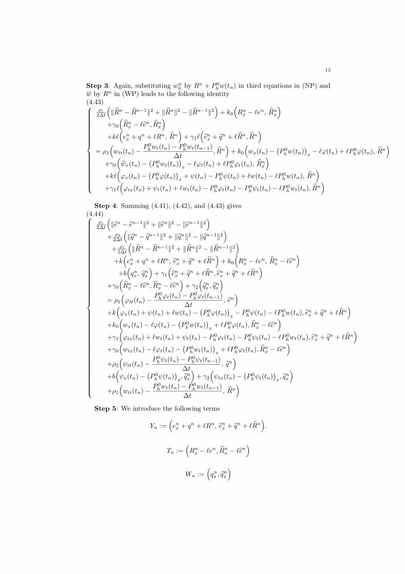
13

Step 3: Again, substituting wnh by Rn + P 0

hw(tn) in third equations in (NP) andw by Rn in (WP) leads to the following identity(4.43)

ρ1

2∆t

(∥Rn − Rn−1∥2 + ∥Rn∥2 − ∥Rn−1∥2

)+ k0

(Rn

x − ℓen, Rnx

)+γ0

(Rn

x − ℓen, Rnx

)+kℓ

(enx + qn + ℓRn, Rn

)+ γ1ℓ

(enx + qn + ℓRn, Rn

)= ρ1

(wtt(tn)−

P 0hwt(tn)− P 0

hwt(tn−1)

∆t, Rn

)+ k0

(wx(tn)−

(P 0hw(tn)

)x− ℓφ(tn) + ℓP 0

hφ(tn), Rn)

+γ0

(wx(tn)−

(P 0hwt(tn)

)x− ℓφt(tn) + ℓP 0

hφt(tn), Rnx

)+kℓ

(φx(tn)−

(P 0hφ(tn)

)x+ ψ(tn)− P 0

hψ(tn) + ℓw(tn)− ℓP 0hw(tn), R

n)

+γ1ℓ(φtx(tn) + ψt(tn) + ℓwt(tn)− P 0

hφt(tn)− P 0hψt(tn)− ℓP 0

hwt(tn), Rn)

Step 4: Summing (4.41), (4.42), and (4.43) gives(4.44)

ρ1

2∆t

(∥en − en−1∥2 + ∥en∥2 − ∥en−1∥2

)+ ρ2

2∆t

(∥qn − qn−1∥2 + ∥qn∥2 − ∥qn−1∥2

)+ ρ1

2∆t

(∥Rn − Rn−1∥2 + ∥Rn∥2 − ∥Rn−1∥2

)+k(enx + qn + ℓRn, enx + qn + ℓRn

)+ k0

(Rn

x − ℓen, Rnx − ℓen

)+b(qnx , q

nx

)+ γ1

(enx + qn + ℓRn, enx + qn + ℓRn

)+γ0

(Rn


)+ γ2

(qnx , q

nx

)= ρ1

(φtt(tn)−

P 0hφt(tn)− P 0

hφt(tn−1)

∆t, en

)+k(φx(tn) + ψ(tn) + ℓw(tn)−

(P 0hφ(tn)

)x− P 0

hψ(tn)− ℓP 0hw(tn), e

nx + qn + ℓRn

)+k0


(P 0hw(tn)

)x+ ℓP 0

hφ(tn), Rnx − ℓen

)+γ1

(φtx(tn) + ℓwt(tn) + ψt(tn)− P 0


hwt(tn), enx + qn + ℓRn

)+γ0

(wtx(tn)− ℓφt(tn)−

(P 0hwt(tn)

)x+ ℓP 0

hφt(tn), Rnx − ℓen

)+ρ2

(ψtt(tn)−

P 0hψt(tn)− P 0

hψt(tn−1)

∆t, qn

)+b(ψx(tn)−

(P 0hψ(tn)

)x, qnx

)+ γ2

(ψtx(tn)−

(P 0hψt(tn)

)x, qnx

)+ρ1

(wtt(tn)−

P 0hwt(tn)− P 0

hwt(tn−1)

∆t, Rn

)Step 5: We introduce the following terms

Yn :=(enx + qn + ℓRn, enx + qn + ℓRn

).

Tn :=(Rn


)Wn :=

(qnx , q

nx

)


From the definitions of en, qn and Rn, we write

Yn =

(enx + qn + ℓRn, enx + qn + ℓRn

)

=

(enx + qn + ℓRn,

enx − en−1x

∆t− (P 0

hφt(tn))x +(P 0

hφ(tn))x − (P 0hφ(tn−1))x

∆t

+qn − qn−1

∆t− P 0

hψt(tn) +P 0hψ(tn)− P 0

hψ(tn−1)

∆t

+ℓ(Rn −Rn−1

∆t− P 0

hwt(tn) +P 0hw(tn)− P 0

hw(tn−1)

∆t

))

=

(enx + qn + ℓRn,

1

∆t

((enx + qn + ℓRn

)−(en−1x + qn−1 + ℓRn−1

))+(P 0


∆t− (P 0

hφt(tn))x

+P 0hψ(tn)− P 0

hψ(tn−1)

∆t− P 0

hψt(tn)

+ℓ(P 0

hw(tn)− P 0hw(tn−1)

∆t− P 0

hwt(tn)))

.

It follows that

Yn =1

2∆t

[∥enx + qn + ℓRn − (en−1

x + qn−1 + ℓRn−1)∥2 + ∥enx + qn + ℓRn∥2 − ∥en−1x + qn−1 + ℓRn−1∥2

]+

(enx + qn + ℓRn, −(P 0

hφt(tn))x +(P 0


∆t

+− P 0hψt(tn) +

P 0hψ(tn)− P 0

hψ(tn−1)

∆t

+ℓ(− P 0

hwt(tn) +P 0hw(tn)− P 0

hw(tn−1)

∆t

))In a similar way, we obtain

(4.45)Tn = 1

2∆t

(∥∥∥Rnx − ℓen − (Rn−1

x − ℓen−1)∥∥∥2 + ∥Rn

x − ℓen∥2 − ∥Rn−1x − ℓRn−1∥2

)+(Rn

x − ℓen,P 0hw(tn)− P 0

hw(tn−1)x∆t

− (P 0hwt(tn))x

)−ℓ(Rn

x − ℓen,P 0hφ(tn)− P 0

hφ(tn−1)

∆t− P 0

hφt(tn),)

and

(4.46)

Wn = 12∆t

(∥qnx − qn−1

x ∥2 + ∥qnx∥2 − ∥qn−1x ∥2

)+(ψx(tn)− ψx(tn−1)

∆t− ψtx(tn), q

nx

).

By inserting the obtained forms of Yn, Tn and Wn in 4.44, we obtain :

15

(4.47)

ρ12∆t

(∥en − en−1∥2 + ∥en∥2 − ∥en−1∥2

)+ρ22∆t

(∥qn − qn−1∥2 + ∥qn∥2 − ∥qn−1∥2

)+ρ12∆t

(∥Rn − Rn−1∥2 + ∥Rn∥2 − ∥Rn−1∥2

)+

k

2∆t

[∥enx + qn + ℓRn − (en−1

x + qn−1 + ℓRn−1)∥2 + ∥enx + qn + ℓRn∥2 − ∥en−1x + qn−1 + ℓRn−1∥2

]+k

((P 0hφ(tn)− P 0

hφ(tn−1))x

∆t− (P 0

hφt(tn))x, enx + qn + ℓRn

)

+k

(P 0hψ(tn)− P 0

hψ(tn−1)

∆t− P 0

hψt(tn), enx + qn + ℓRn

)

+kℓ

(P 0hw(tn)− P 0

hw(tn−1)

∆t− P 0

hwt(tn), enx + qn + ℓRn

)

+k02∆t

(∥Rn

x − ℓen −(Rn−1

x − ℓen−1)∥2 + ∥Rn

x − ℓen∥2 − ∥Rn−1x − ℓen−1∥2

)

+k0

((P 0hw(tn)− P 0

hw(tn−1))x

∆t−(P 0hwt(tn)

)x, Rn

x − ℓen

)

−k0ℓ

(P 0hφ(tn)− P 0

hφ(tn−1)

∆t− P 0


)

+b

2∆t

(∥qnx − qn−1

x ∥2 + ∥qnx∥2 − ∥qn−1x ∥2

)+ b

(ψx(tn)− ψx(tn−1)

∆t− ψtx(tn), q

nx

)+γ1∥enx + ℓRn + qn∥2 + γ0∥Rn

x − ℓen∥2 + γ2∥qnx∥2 =

ρ1

(φtt(tn)−

P 0hφt(tn)− P 0

hφ(tn−1)

∆t, en

)

+k

(φx(tn) + ψ(tn) + ℓw(tn)−

(P 0hφ(tn)

)x− P 0

hψ(tn)− ℓP 0hw(tn) , e

nx + qn + ℓRn

)

+k0


(P 0hw(tn)

)x+ ℓP 0


)

+γ1



hwt(tn) , enx + qn + ℓRn

)

+γ0


(P 0hwt(tn)

)x+ ℓP 0


)

+ρ2

(ψtt(tn)−

P 0hψt(tn)− P 0

hψt(tn−1)

∆t, qn

)+ b

(ψx(tn)−

(P 0hψ(tn)

)x, qnx

)

+ρ1

(wtt(tn)−

P 0hwt(tn)− P 0

hwt(tn−1)

∆t, Rn

)+ γ2

(ψtx(tn)−

(P 0hψt(tn)

)x, qnx

)Step 6: By taking into consideration that ∥enx+qn+ℓRn−(en−1

x +qn−1+ℓRn−1)∥2,∥en − en−1∥2, ∥qn − qn−1∥2, ∥Rn − Rn−1∥2, ∥Rn

x − ℓen −(Rn−1

x − ℓen−1)∥2,


∥qnx − qn−1x ∥2 are positive and rearranging some terms in 4.48, we get

(4.48)

ρ12∆t

(∥en∥2 − ∥en−1∥2

)+

ρ22∆t

(∥qn∥2 − ∥qn−1∥2

)+

ρ12∆t

(∥Rn∥2 − ∥Rn−1∥2

)+

k

2∆t

[∥enx + qn + ℓRn∥2 − ∥en−1

x + qn−1 + ℓRn−1∥2]

+k02∆t

(∥Rn

x − ℓen∥2 − ∥Rn−1x − ℓen−1∥2

)

+b

2∆t

(∥qnx∥2 − ∥qn−1

x ∥2)

+γ1∥enx + ℓRn + qn∥2 + γ0∥Rnx − ℓen∥2 + γ2∥qnx∥2 ≤

k

((P 0

hφt(tn))x −

(P 0hφ(tn)− P 0

hφ(tn−1))x

∆t, enx + qn + ℓRn

)

+k

(P 0hψt(tn)−

P 0hψ(tn)− P 0

hψ(tn−1)


)

+kℓ

(P 0hwt(tn)−

P 0hw(tn)− P 0

hw(tn−1)


)

+b

(ψtx(tn)−

ψx(tn)− ψx(tn−1)

∆t, qnx

)

+k0

((P 0hwt(tn)

)x−(P 0hw(tn)− P 0

hw(tn−1))x

∆t, Rn

x − ℓen

)

+k0ℓ

(P 0hφ(tn)− P 0

hφ(tn−1)

∆t− P 0


)

+ρ1

(φtt(tn)−

P 0hφt(tn)− P 0

hφ(tn−1)

∆t, en

)

+k


(P 0hφ(tn)

)x− P 0


nx + qn + ℓRn

)

+k0


(P 0hw(tn)

)x+ ℓP 0


)

+γ1




)

+γ0


(P 0hwt(tn)

)x+ ℓP 0


)

+ρ2

(ψtt(tn)−

P 0hψt(tn)− P 0

hψt(tn−1)

∆t, qn

)+ b

(ψx(tn)−

(P 0hψ(tn)

)x, qnx

)

+ρ1

(wtt(tn)−

P 0hwt(tn)− P 0

hwt(tn−1)

∆t, Rn

)+ γ2

(ψtx(tn)−

(P 0hψt(tn)

)x, qnx

)

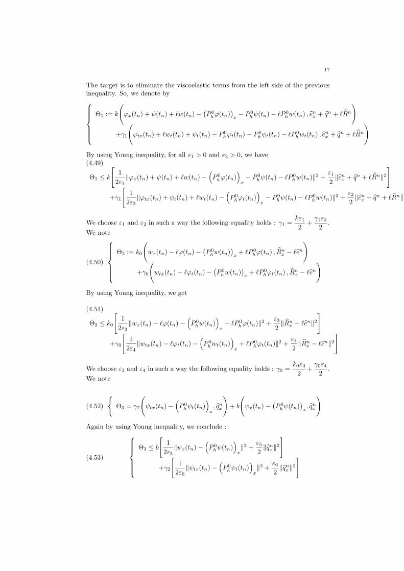
17

The target is to eliminate the viscoelastic terms from the left side of the previousinequality. So, we denote by

Θ1 := k


(P 0hφ(tn)

)x− P 0


nx + qn + ℓRn

)

+γ1




)

By using Young inequality, for all ε1 > 0 and ε2 > 0, we have(4.49)

Θ1 ≤ k

[1

2ε1∥φx(tn) + ψ(tn) + ℓw(tn)−

(P 0hφ(tn)

)x− P 0

hψ(tn)− ℓP 0hw(tn)∥2 +

ε12∥enx + qn + ℓRn∥2

]

+γ1

[1

2ε2∥φtx(tn) + ψt(tn) + ℓwt(tn)−

(P 0hφt(tn)

)x− P 0

hψ(tn)− ℓP 0hw(tn)∥2 +

ε22∥enx + qn + ℓRn∥2

]

We choose ε1 and ε2 in such a way the following equality holds : γ1 =kε12

+γ1ε22

.We note

(4.50)

Θ2 := k0


(P 0hw(tn)

)x+ ℓP 0

hφ(tn) , Rnx − ℓen

)

+γ0


(P 0hw(tn)

)x+ ℓP 0

hφt(tn) , Rnx − ℓen

)

By using Young inequality, we get

(4.51)

Θ2 ≤ k0

[1

2ε3∥wx(tn)− ℓφ(tn)−

(P 0hw(tn)

)x+ ℓP 0

hφ(tn)∥2 +ε32∥Rn

x − ℓen∥2]

+γ0

[1

2ε4∥wtx(tn)− ℓφt(tn)−

(P 0hwt(tn)

)x+ ℓP 0

hφt(tn)∥2 +ε42∥Rn

x − ℓen∥2]

We choose ε3 and ε4 in such a way the following equality holds : γ0 =k0ε32

+γ0ε42

.We note

(4.52)

Θ3 = γ2

(ψtx(tn)−

(P 0hψt(tn)

)x, qnx

)+ b

(ψx(tn)−

(P 0hψ(tn)

)x, qnx

)

Again by using Young inequality, we conclude :

(4.53)

Θ3 ≤ b

[1

2ε5∥ψx(tn)−

(P 0hψ(tn)

)x∥2 + ε5

2∥qnx∥2

]

+γ2

[1

2ε6∥ψtx(tn)−

(P 0hψt(tn)

)x∥2 + ε6

2∥qnx∥2

]


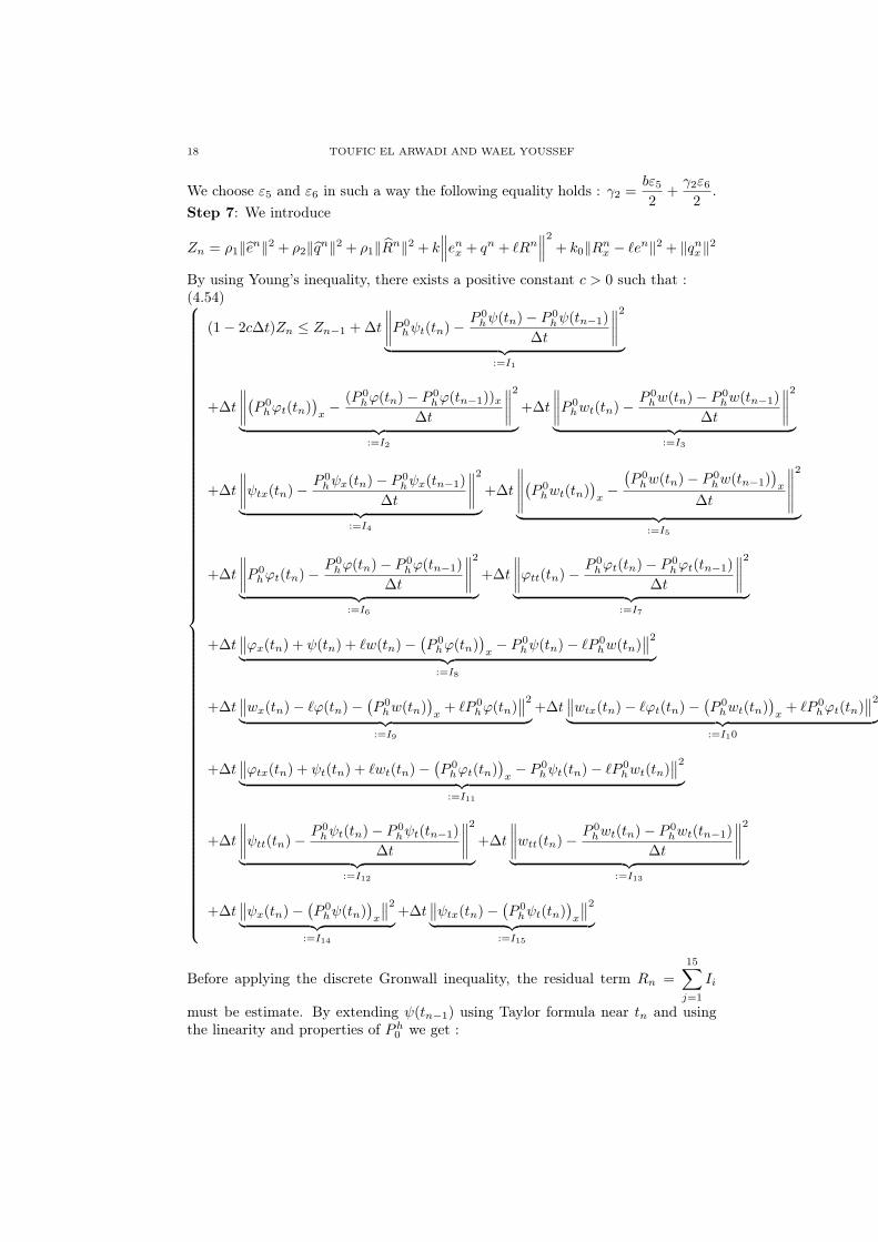
We choose ε5 and ε6 in such a way the following equality holds : γ2 =bε52

+γ2ε62

.Step 7: We introduce

Zn = ρ1∥en∥2 + ρ2∥qn∥2 + ρ1∥Rn∥2 + k∥∥∥enx + qn + ℓRn

∥∥∥2 + k0∥Rnx − ℓen∥2 + ∥qnx∥2

By using Young’s inequality, there exists a positive constant c > 0 such that :(4.54)

(1− 2c∆t)Zn ≤ Zn−1 +∆t

∥∥∥∥P 0hψt(tn)−

P 0hψ(tn)− P 0

hψ(tn−1)

∆t

∥∥∥∥2︸︷︷︸:=I1

+∆t

∥∥∥∥(P 0hφt(tn)

)x− (P 0

hφ(tn)− P 0hφ(tn−1))x

∆t

∥∥∥∥2︸︷︷︸:=I2

+∆t

∥∥∥∥P 0hwt(tn)−

P 0hw(tn)− P 0

hw(tn−1)

∆t

∥∥∥∥2︸︷︷︸:=I3

+∆t

∥∥∥∥ψtx(tn)−P 0hψx(tn)− P 0

hψx(tn−1)

∆t

∥∥∥∥2︸︷︷︸:=I4

+∆t

∥∥∥∥∥(P 0hwt(tn)

)x−(P 0hw(tn)− P 0

hw(tn−1))x

∆t

∥∥∥∥∥2

︸︷︷︸:=I5

+∆t

∥∥∥∥P 0hφt(tn)−

P 0hφ(tn)− P 0

hφ(tn−1)

∆t

∥∥∥∥2︸︷︷︸:=I6

+∆t

∥∥∥∥φtt(tn)−P 0hφt(tn)− P 0

hφt(tn−1)

∆t

∥∥∥∥2︸︷︷︸:=I7

+∆t∥∥φx(tn) + ψ(tn) + ℓw(tn)−

(P 0hφ(tn)

)x− P 0

hψ(tn)− ℓP 0hw(tn)

∥∥2︸︷︷︸:=I8

+∆t∥∥wx(tn)− ℓφ(tn)−

(P 0hw(tn)

)x+ ℓP 0

hφ(tn)∥∥2︸︷︷︸

:=I9

+∆t∥∥wtx(tn)− ℓφt(tn)−

(P 0hwt(tn)

)x+ ℓP 0

hφt(tn)∥∥2︸︷︷︸

:=I10

+∆t∥∥φtx(tn) + ψt(tn) + ℓwt(tn)−

(P 0hφt(tn)

)x− P 0

hψt(tn)− ℓP 0hwt(tn)

∥∥2︸︷︷︸:=I11

+∆t

∥∥∥∥ψtt(tn)−P 0hψt(tn)− P 0

hψt(tn−1)

∆t

∥∥∥∥2︸︷︷︸:=I12

+∆t

∥∥∥∥wtt(tn)−P 0hwt(tn)− P 0

hwt(tn−1)

∆t

∥∥∥∥2︸︷︷︸:=I13

+∆t∥∥ψx(tn)−

(P 0hψ(tn)

)x

∥∥2︸︷︷︸:=I14

+∆t∥∥ψtx(tn)−

(P 0hψt(tn)

)x

∥∥2︸︷︷︸:=I15

Before applying the discrete Gronwall inequality, the residual term Rn =

15∑j=1

Ii

must be estimate. By extending ψ(tn−1) using Taylor formula near tn and usingthe linearity and properties of Ph

0 we get :

19

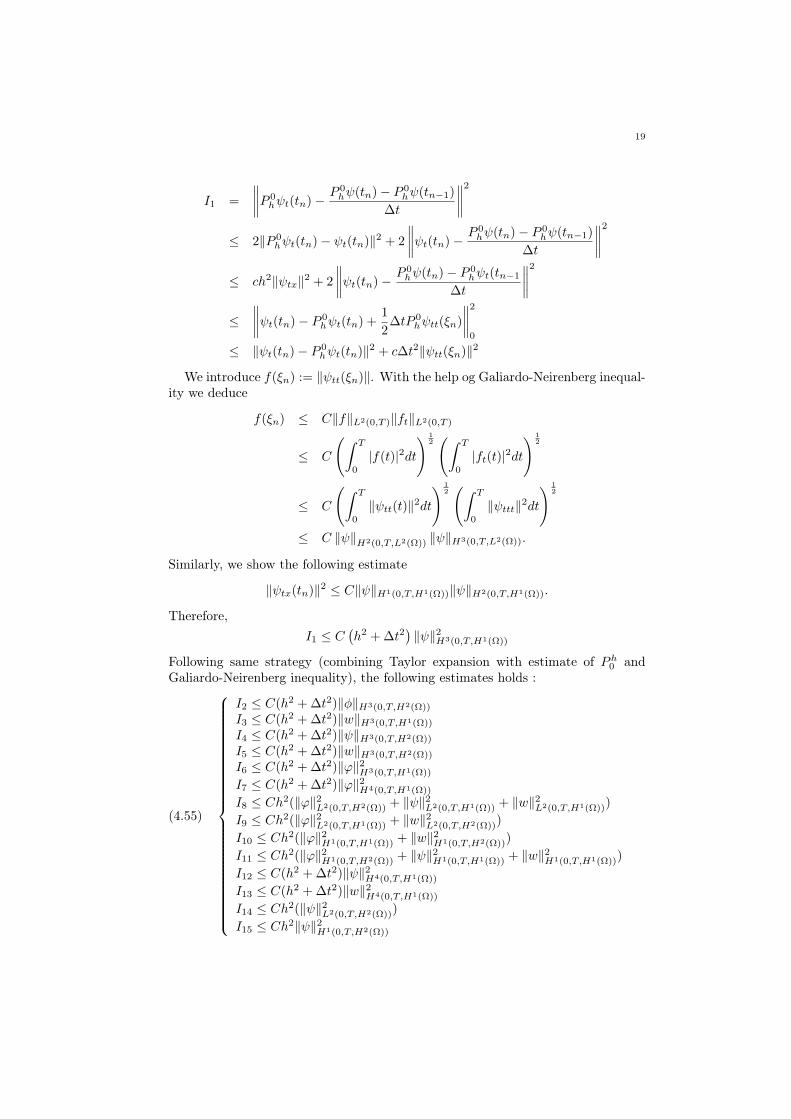
I1 =

∥∥∥∥P 0hψt(tn)−

P 0hψ(tn)− P 0

hψ(tn−1)

∆t

∥∥∥∥2≤ 2∥P 0

hψt(tn)− ψt(tn)∥2 + 2

∥∥∥∥ψt(tn)−P 0hψ(tn)− P 0

hψ(tn−1)

∆t

∥∥∥∥2≤ ch2∥ψtx∥2 + 2

∥∥∥∥ψt(tn)−P 0hψ(tn)− P 0

hψt(tn−1

∆t

∥∥∥∥2≤

∥∥∥∥ψt(tn)− P 0hψt(tn) +

1

2∆tP 0

hψtt(ξn)

∥∥∥∥20

≤ ∥ψt(tn)− P 0hψt(tn)∥2 + c∆t2∥ψtt(ξn)∥2

We introduce f(ξn) := ∥ψtt(ξn)∥. With the help og Galiardo-Neirenberg inequal-ity we deduce

f(ξn) ≤ C∥f∥L2(0,T )∥ft∥L2(0,T )

≤ C

(∫ T

0

|f(t)|2dt

) 12(∫ T

0

|ft(t)|2dt

) 12

≤ C

(∫ T

0

∥ψtt(t)∥2dt

) 12(∫ T

0

∥ψttt∥2dt

) 12

≤ C ∥ψ∥H2(0,T,L2(Ω)) ∥ψ∥H3(0,T,L2(Ω)).

Similarly, we show the following estimate

∥ψtx(tn)∥2 ≤ C∥ψ∥H1(0,T,H1(Ω))∥ψ∥H2(0,T,H1(Ω)).

Therefore,I1 ≤ C

(h2 +∆t2

)∥ψ∥2H3(0,T,H1(Ω))

Following same strategy (combining Taylor expansion with estimate of Ph0 and

Galiardo-Neirenberg inequality), the following estimates holds :

(4.55)

I2 ≤ C(h2 +∆t2)∥ϕ∥H3(0,T,H2(Ω))

I3 ≤ C(h2 +∆t2)∥w∥H3(0,T,H1(Ω))

I4 ≤ C(h2 +∆t2)∥ψ∥H3(0,T,H2(Ω))

I5 ≤ C(h2 +∆t2)∥w∥H3(0,T,H2(Ω))

I6 ≤ C(h2 +∆t2)∥φ∥2H3(0,T,H1(Ω))

I7 ≤ C(h2 +∆t2)∥φ∥2H4(0,T,H1(Ω))

I8 ≤ Ch2(∥φ∥2L2(0,T,H2(Ω)) + ∥ψ∥2L2(0,T,H1(Ω)) + ∥w∥2L2(0,T,H1(Ω)))

I9 ≤ Ch2(∥φ∥2L2(0,T,H1(Ω)) + ∥w∥2L2(0,T,H2(Ω)))

I10 ≤ Ch2(∥φ∥2H1(0,T,H1(Ω)) + ∥w∥2H1(0,T,H2(Ω)))

I11 ≤ Ch2(∥φ∥2H1(0,T,H2(Ω)) + ∥ψ∥2H1(0,T,H1(Ω)) + ∥w∥2H1(0,T,H1(Ω)))

I12 ≤ C(h2 +∆t2)∥ψ∥2H4(0,T,H1(Ω))

I13 ≤ C(h2 +∆t2)∥w∥2H4(0,T,H1(Ω))

I14 ≤ Ch2(∥ψ∥2L2(0,T,H2(Ω)))

I15 ≤ Ch2∥ψ∥2H1(0,T,H2(Ω))


By denoting Rn =

1∑i=1

5Ii, and using the estimates of Ii, we get

(1− 2c∆t)Zn ≤ Zn−1 + C∆t(h2 +∆t2)

Taking into consideration that nδt ≤ T and applying the discrete Gronwall lemmaleads to the end of the proof.

References

[1] F. Alabau; J. M. Rivera, D.S. Amedia Junior, Stability to Weak Dissipative Bresse System,Journal of Math. Analy. and Appl. 374 (2), pp.481-498 (2011).

[2] J. Ahn, D.E. Stewart, A viscoelastic Timoshenko beam with dynamic frictionless impact,Discrete Contin. Dyn. Syst. Ser. B 12 (1) (2009) 122.

[3] M. Afilal; A. Guesmia; A. Soufyane, New Stability Results for a Linear ThermoelasticBresse System with Second Sound, (2019) Applied Mathematics and Optimization, DOI:10.1007/s00245-019-09560-7.

[4] C. Bernardi; M. Copetti, Discretization of a nonlinear dynamic thermoviscoelastic Timo-shenko beam model, ZAMM. Z. Angew. Math. Mech. 1-18 (2016).

[5] J.A.C. BRESSE, Cours de Mécanique Appliquée, Mallet Bachelier, 1859.[6] M. Copetti; J.R. Fernàndez, A dynamic contact problem involving a Timoshenko beam model

(2013), 117-128.[7] S. Chen, K. Liu and Z. Liu, Spectrum and stability of elastic systems with global or local

Kelvin-Voigt damping, SIAM J. Appl. Math. 59 (1998), 651-668.[8] M. Crouzeix, J. Rappaz, On Numerical Approximation in Bifurcation Theory, Masson 1990.[9] S. Ervedoza; Chuang Zheng; E. Zuazua, On the observability of time-discrete conservative

linear systems, Journal of Functional Analysis, Volume 254, Issue 12, (2008), 3037-3078.[10] A. Guesmia, M. Kafini, Bresse system with infinite memories, Math. Meth. Appl. Sci., (2015),

2389-2402.[11] A. Guesmia; M. Kirane, Uniform and weak stability of Bresse system with two infinite mem-

ories, Z. Angew. Math. Phys. (2016), 67-124.[12] A. Guesmia; S.A. Massaoudi, On the control of a viscoelastic damped Timoshenko-type

system, (2008) Applied Mathematics and Computation 589-597.[13] A. Guesmia; S.A. Massaoudi, General energy decay estimates of Timoshenko systems with

frictional versus viscoelastic damping, (2009) Mathematical Methods in the Applied Sciences2102-2122.

[14] A. Haraux, Semi-groupes lineéaires et eéquations d’évolution lineéaires peériodiques. Publi-cation du Laboratoire d’Analyse Numeérique No. 78011, Universiteé Pierre et Marie Curie,Paris, 1978.

[15] A. Keddi; T. Apalara; S. Messaoudi, Exponential and Polynomial Decay in a Thermoelastic-Bresse System with Second Sound, (2018) 77: 315-341.

[16] V. Komornik, Exact controllability and stabilization. The Multiplier Method, RAM Res.Appl.Math., Masson, Paris, John Wiley, Chicester, UK, 1994. (1

[17] V. KOMORNIK, Exact controllability and stabilization. The Multiplier Method, RAM Res.Appl.Math., Masson, Paris, John Wiley, Chicester, UK, 1994.

[18] S. Massaoudi; J. Hashem Hassan, Neu general decay results in a finite-memory Bresse system,Communications on pure and applied analysis, (2019) 1637-1662.

[19] J. Lagnese, Boundary Stabilization of Thin Plates, SIAM Studies in Appl. Math., Philadel-phia, 1989.

[20] J.E. Lagnese, G. Leugering, J.P.G. Schmidt, Modelling Analysis and Control of DynamicElastic Multi-Link Structures, Systems Control Found. Appl., 1994.

[21] J. L. LIONS, Contrôlabilité exacte et stabilisation de systèmes distribués, Vol. 1, Masson,Paris, 1988.

[22] J. L. LIONS, Contrôlabilité exacte et stabilisation de systèmes distribués, Vol. 2, Masson,Paris, 1988.

[23] S. Chen, K. Liu and Z. Liu, Spectrum and stability of elastic systems with global or localKelvin-Voigt damping, SIAM J. Appl. Math. 59 (1998), 651-668.

21

[24] K. Liu and Z. Liu, Exponential decay of energy of the Euler-Bernoulli beam with locallydistributed Kelvin-Voigt damping, SIAM J. Cont. Optim 36(3) (1998), 1086-1098.

[25] D. LI; C. ZHANG; Q. HU; H. ZHANG, Energy Decay Rate of Bresse System with NonlinearLocalized Damping, British Journal of Math. & Computer Science 4(12): 1665-1677 (2014).

[26] L.H. FATORI; R.N. MONTEIRO, The Optimal Decay Rate for a Weak Dissipative BresseSystem, App. Math. Letters 25 (2012), 600 - 604.

[27] M. Rincon; M. Copetti, Numerical analysis for a locally damped wave equation, Jornal ofApp. Analy. and Computation (2013), 169-182.

[28] N. Tatar, Stabilization of a viscoelastic Timoshenko beam. Applicable Analysis (2013), 92(1),27-43.

[29] A. WEHBE; W. YOUSSEF, Stabilization of the uniform Timoshenko beam by one locallydistributed feedback, Applicable Analysis, (2009), 7, 1067 - 1078.

[30] A. WEHBE; W. YOUSSEF, Exponential and Polynomial Stability of an Elastic Bresse Sys-tem with two Locally Distributed Feedbacks, Jornal of Math. Phy. JMP 51, 103523 (2010).

Toufic EL Arwadi, Beirut Arab University, Department of mathematics and com-puter science, Debbieh, Lebanon

E-mail address: [email protected]

Wael Youssef, Lebanese University, Faculty of Sciences, Hadath, Beyrouth, LebanonE-mail address: [email protected]

Documents

ON THE STABILIZATION OF THE BRESSE BEAM WITH KELVIN …