ON THE STABILITY OF EARTH’S TROJANS

C. LHOTKA1, L.Y. ZHOU2, R. DVORAK3

1 Departement de MathematiqueRempart de la Vierge 8, B-5000 Namur, Belgiumemail: clhotka@fundp.ac.be2 Departement of Astronomy, Nanjing UniversityNanjing, 210093, China3 Institute for Astronomy, University of ViennaTurkenschanzstraße 17, A-1180 Vienna, Austria

ABSTRACT. The gas giants Jupiter and Neptune are known to host Trojans, and also Mars hasco-orbiting asteroids. Recently, in an extensive numerical investigation ([8]) the possibility of capturesof asteroids by the terrestrial planets and even the Earth into the 1:1 mean motion resonance (MMR)was studied. The first Earth Trojan has been observed ([2]) and found to be in a so-called tadpoleorbit closed to the Lagrange point L4. We did a detailed study of the actual orbit of this Trojan 2010TK7 including the study of clone orbits, derived an analytical mapping in a simplified dynamical system(Sun+Earth+massless asteroid) and studied the phase space structure of the Earth’s Lagrange points withrespect to the eccentricities and the inclinations of a large number of fictitious Trojans. The extension ofstable zones around the Lagrange points is established with the aid of dynamical mappings; the knownTrojan 2010 TK7 finds himself inside an unstable zone.

1. INTRODUCTION

Trojan asteroids move in the same orbits as their host planets, but around 60 degrees ahead or 60degrees behind them close to the so-called Lagrange points L4 or L5. Up to now we observe Trojansof Jupiter (about 4000), of Neptune (7) and also of Mars (3) but the other planets still seem to lack ofsuch a companion (e.g. [9]). Although in the original paper of the first confirmed discovery of a Trojanasteroid ([2]) a dynamical study has been undertaken we extended it to a more detailed investigation. Wemake use of a dynamical symplectic mapping of the Sun-Earth Trojan model and of extensive numericalintegrations of fictitious Trojans in the full model of our Solar system. With this approach we were ableto obtain a deeper understanding of the dynamical aspects of the first confirmed Earth Trojan asteroid2010 TK7 as well as the stability of Earth Trojan asteroids in general.

2. THE REAL ORBIT OF 2010 TK7

The orbit of the asteroid 2010 TK7 is numerically simulated to obtain a direct estimation of itsorbital stability and its origin. After some test runnings and comparisons between different numericalcodes, we choose the Mercury6 integrator package ([1]) to make our simulations in this part. For theinitial conditions of 2010 TK7, we adopt the data listed in the AstDyS website1. Specifically, at epochJD2455800.5, the semi-major axis a = 1.00037AU, eccentricity e = 0.190818, inclination i = 20.88,ascending node Ω = 96.539, perihelion argument ω = 45.846 and the mean anomaly M = 217.329.Since the errors are unavoidable in the observation and orbital determination, we simultaneously simulatethe evolution of a cloud of 100 clone orbits within the error bars. These clone orbits are generated usingthe covariance matrix listed in the AstDyS website. Two dynamical models are applied. In one model,we include the Sun and eight planets from Mercury to Neptune and the Earth is placed in the barycenterof the Earth-Moon system and its mass is replaced by the combined mass of the system. In the othermodel however, the Earth and the Moon are treated separately. Hereafter the former and later models aredenoted by EMB and E+M, respectively. In two dynamical models, we integrate the nominal and clone

1http://newton.dm.unipi.it

221

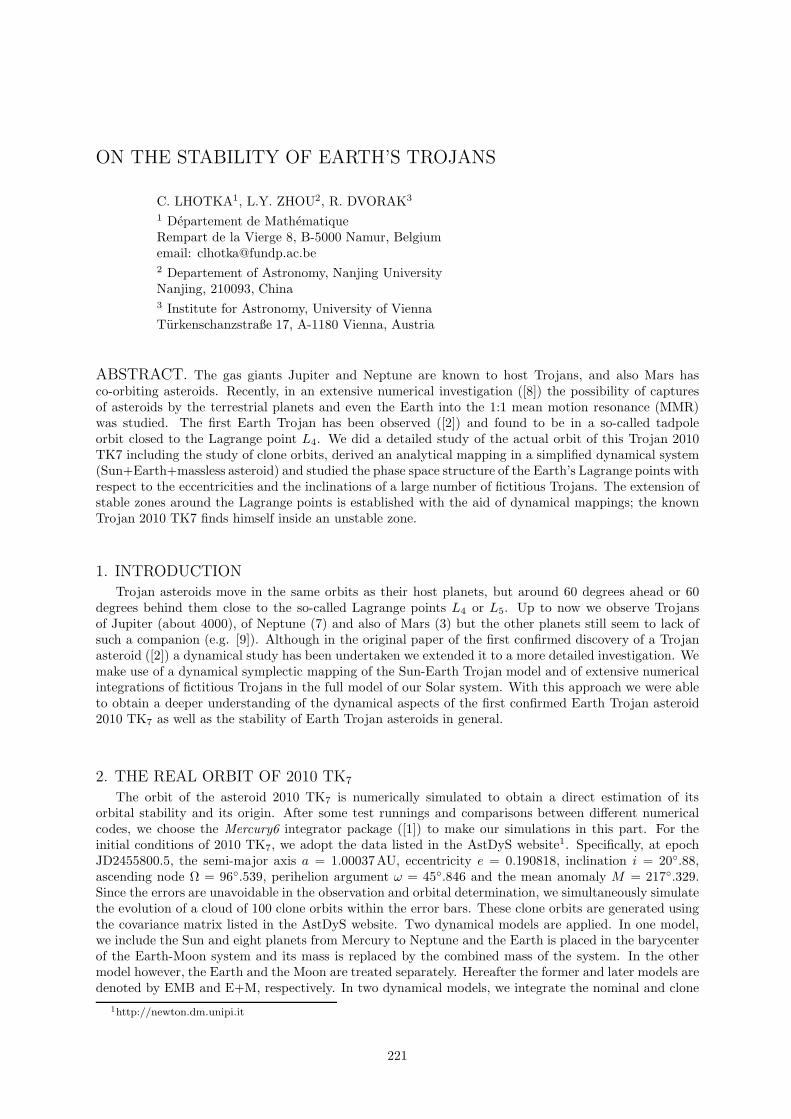
orbits both forward (to future) and backward (to past) for 1 million years. During the integration, wecheck the resonant angle δλ = λ − λEMB (the difference between the mean longitude of the asteroid andthe barycenter of the Earth-Moon system). At the start of integration (t = 0), the δλ librates around60 since 2010 TK7 is on a tadpole orbit around L4 right now. But it may leave this region in bothbackward and forward integrations. We record the moment t1 when δλ reaches 180 for the first time,and the moment t2 when δλ attains 360. So t1 and t2 are the time when an asteroid escapes from theL4 tadpole region and from the 1:1 MMR. Figure1 summarizes the distribution of t1 and t2.

Figure 1: The time when clone asteroids escape from the L4 region (t1) and from the 1:1 MMR (t2).

From the distribution of t1 and t2, we conclude that the two models EMB and E+M are consistentwith each other, they do not make considerable differences. It is more or less a natural consequence ofthe Earth and the Moon being a close binary. From Figure 1, we can also conclude that 2010 TK7 is atemporal Earth Trojan. In fact the nominal orbit will leave the L4 region in about 17000 years, whilemost of the clone orbits will escape in ∼ 15000 years. The results of backward integration show that mostof the clones became L4 Earth Trojans only about 1700 years ago, just as the nominal orbit did. As forthe time they leave the 1:1 MMR, it is ∼ 4.0× 104 years in the past and ∼ 2.5× 105 years in the future.The total time for this object being in the 1:1 MMR with the Earth is less than ∼ 3.0 × 105 years.

3. THE ANALYTICAL MAPPING

The most basic dynamical model behind the motion of 2010 TK7 takes the form:

H = HKep + T + µ′R(a, e, i, ω,Ω, M, M ′; P ′) . (1)

Here HKep defines the motion of the asteroid around the Sun and µ′R gives the potential of the Earthwith mass µ′. Here M ′ denotes the mean anomaly of the Earth. R is time dependent due to the presenceof M ′, we therefore extend the phase space with T (assuming, that the mean motion n′ of the Earth isequal to one). Moreover, we denote by P ′ the orbital parameters of the Earth P ′ = (a′, e′, i′, ω′, Ω′). Inthe further discussion we use the modified Delaunay variables λ1 = M + ω + Ω, λ2 = −ω − Ω, λ3 = −Ωand their conjugated momenta Λ1 =

√a, Λ2 =

√a(1−

√1 − e2), Λ3 = 2

√a√

1 − e2 sin2(i/2) and similarfor the orbital parameters of the Earth. Moreover, we write Λ = (Λ1, Λ2, Λ3) and λ = (λ1, λ2, λ3) inshort. The aim of this section is to investigate the role of P ′ on the mean orbit of the asteroid 2010 TK7.For this reason we will make use of a symplectic mapping based on the averaged Hamiltonian ([6]):

H = −1

2Λ21

+1

2π

∫ 2π

0

µ′R (Λ, τ, λ2, λ3, λ′

1; P′) dλ′

1 , (2)

where τ = λ1 − λ′

1 is the resonant angle (which is also related to δλ of the previous section). Thus, theaverage over the fast angle λ′

1 defines the mean dynamics close to the 1 : 1 MMR. To shorten notationwe will write λ = (τ, λ2, λ3) from now on. Based on Equation (2) we define a transformation from state(λ(k), Λ(k)) to (λ(k+1), Λ(k+1)) via the generating function:

WP ′ = WP ′

(

λ(k), Λ(k+1); P ′

)

= λ(k) · Λ(k+1) + 2πH(

λ(k), Λ(k+1); P ′

)

.

Based on it the mapping from time k to k + 1 is given by:

λ(k+1)j =

∂WP ′

∂Λ(k+1)j

, Λ(k)j =

∂WP ′

∂λ(k)j

with j = 1, 2, 3 . (3)

222

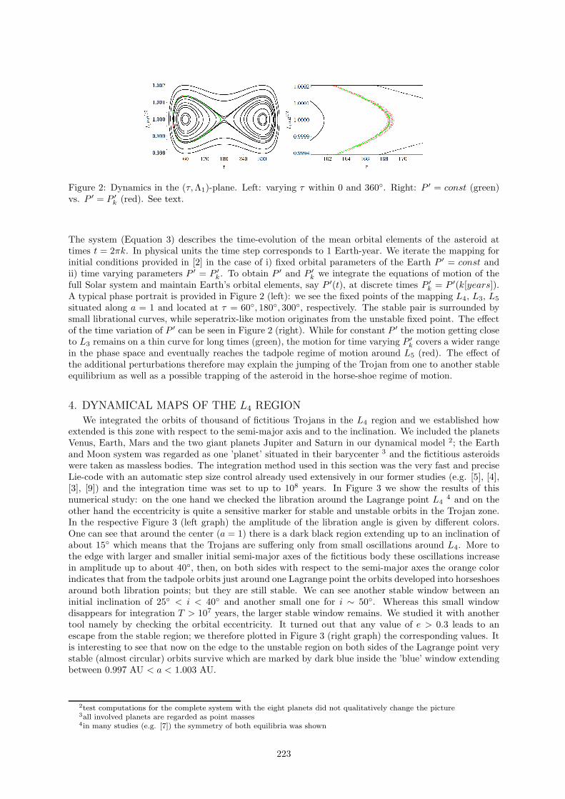
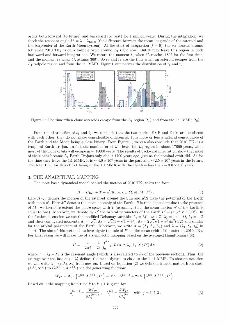
Figure 2: Dynamics in the (τ, Λ1)-plane. Left: varying τ within 0 and 360. Right: P ′ = const (green)vs. P ′ = P ′

k (red). See text.

The system (Equation 3) describes the time-evolution of the mean orbital elements of the asteroid attimes t = 2πk. In physical units the time step corresponds to 1 Earth-year. We iterate the mapping forinitial conditions provided in [2] in the case of i) fixed orbital parameters of the Earth P ′ = const andii) time varying parameters P ′ = P ′

k. To obtain P ′ and P ′

k we integrate the equations of motion of thefull Solar system and maintain Earth’s orbital elements, say P ′(t), at discrete times P ′

k = P ′(k[years]).A typical phase portrait is provided in Figure 2 (left): we see the fixed points of the mapping L4, L3, L5

situated along a = 1 and located at τ = 60, 180, 300, respectively. The stable pair is surrounded bysmall librational curves, while seperatrix-like motion originates from the unstable fixed point. The effectof the time variation of P ′ can be seen in Figure 2 (right). While for constant P ′ the motion getting closeto L3 remains on a thin curve for long times (green), the motion for time varying P ′

k covers a wider rangein the phase space and eventually reaches the tadpole regime of motion around L5 (red). The effect ofthe additional perturbations therefore may explain the jumping of the Trojan from one to another stableequilibrium as well as a possible trapping of the asteroid in the horse-shoe regime of motion.

4. DYNAMICAL MAPS OF THE L4 REGION

We integrated the orbits of thousand of fictitious Trojans in the L4 region and we established howextended is this zone with respect to the semi-major axis and to the inclination. We included the planetsVenus, Earth, Mars and the two giant planets Jupiter and Saturn in our dynamical model 2; the Earthand Moon system was regarded as one ’planet’ situated in their barycenter 3 and the fictitious asteroidswere taken as massless bodies. The integration method used in this section was the very fast and preciseLie-code with an automatic step size control already used extensively in our former studies (e.g. [5], [4],[3], [9]) and the integration time was set to up to 108 years. In Figure 3 we show the results of thisnumerical study: on the one hand we checked the libration around the Lagrange point L4

4 and on theother hand the eccentricity is quite a sensitive marker for stable and unstable orbits in the Trojan zone.In the respective Figure 3 (left graph) the amplitude of the libration angle is given by different colors.One can see that around the center (a = 1) there is a dark black region extending up to an inclination ofabout 15 which means that the Trojans are suffering only from small oscillations around L4. More tothe edge with larger and smaller initial semi-major axes of the fictitious body these oscillations increasein amplitude up to about 40, then, on both sides with respect to the semi-major axes the orange colorindicates that from the tadpole orbits just around one Lagrange point the orbits developed into horseshoesaround both libration points; but they are still stable. We can see another stable window between aninitial inclination of 25 < i < 40 and another small one for i ∼ 50. Whereas this small windowdisappears for integration T > 107 years, the larger stable window remains. We studied it with anothertool namely by checking the orbital eccentricity. It turned out that any value of e > 0.3 leads to anescape from the stable region; we therefore plotted in Figure 3 (right graph) the corresponding values. Itis interesting to see that now on the edge to the unstable region on both sides of the Lagrange point verystable (almost circular) orbits survive which are marked by dark blue inside the ’blue’ window extendingbetween 0.997 AU < a < 1.003 AU.

2test computations for the complete system with the eight planets did not qualitatively change the picture3all involved planets are regarded as point masses4in many studies (e.g. [7]) the symmetry of both equilibria was shown

223

’all-0-56-s’

0.995 0.996 0.997 0.998 0.999 1 1.001 1.002 1.003 1.004 1.005

semimajor axes

0

10

20

30

40

50

incl

inat

ion

0

20

40

60

80

100

120

140

160

180

0.997 0.998 0.999 1 1.001 1.002 1.003

semimajor axes

26

28

30

32

34

36

38

40

incl

inat

ion

0.1

0.2

0.3

0.4

0.5

0.6

0.7

0.8

0.9

1

Figure 3: Dynamical map of the L4 region. Left: the libration amplitudes of the fictitious Trojans;tadpole orbits are inside the red line in dark blue and violet close to the center, horseshoe orbits arein orange, escapers in light yellow. Right: maximum eccentricity of the Trojans within 107 years ofintegration; stable orbits are shown in dark blue, escaping orbits are marked from orange to yellow.

5. CONCLUSIONS

In this study we confirm that the recently discovered Earth Trojan 2010 TK7 is a temporarily capturedasteroid, which is stable only for several thousand years. In its actual orbit it is in a tadpole orbit aroundL4, but it is a jumping Trojan changing its orbit between tadpole around one or the other equilibriumpoint and horseshoe orbits; but then it escapes from the stable region. This dynamical behaviour isobserved in backward as well in forward integration and well confirmed by all three methods used inthe paper. Two main stable regions were found. One for low inclined orbits (i < 15) and one for25 < i < 40. Surprisingly is that the Trojan discovered by recent observations is in none of these stableregions but well inside an unstable zone! But we may be able in future to observe many more of thesecompanions of the Earth.

Acknowledgements. ZLY thanks the financial support by the National Natural Science Foundation ofChina (No. 10833001, 11073012, 11078001).

6. REFERENCES

[1] Chambers, J., 1999, ”A hybrid symplectic integrator that permits close encounters between massivebodies”, MNRAS , 304, 793–799.

[2] Connors, M., Wiegert, P., Veillet, C., 2011, ”Earth’s Trojan asteroid”, Nature, Vol.475, 481-483.[3] Dvorak, R., Bazso, A., Zhou, L.-Y., 2010, ”Where are the Uranus Trojans?”, Celest. Mech. Dyn.

Astr. 107, 1–15.[4] Dvorak, R., Lhotka, Ch., Schwarz, R., 2008, ”The dynamics of inclined Neptune Trojans”, Celest.

Mech. Dyn. Astr. 102, 97–110.[5] Dvorak, R., Pilat-Lohinger, E., Schwarz, R., Freistetter, F, 2004, ”Extrasolar Trojan Planets close to

habitable zones”, A&A 426, L37–L40.[6] Lhotka, C., Efthymiopoulos, C., Dvorak, R., 2008, ”Nekhoroshev stability at L4 or L5 in the elliptic-

restricted three-body problem - application to Trojan asteroids” MNRAS 384, 1165–1177.[7] Nesvorny, D., Dones, L., 2002, ”How Long-Lived Are the Hypothetical Trojan Populations of Saturn,

Uranus, and Neptune?”, Icarus 160, 271–288.[8] Schwarz, R., Dvorak, R., 2011, ”On the Capture of Asteroids by Venus, Earth and Mars into the 1:1

Mean Motion Resonance”, Celest. Mech. Dyn. Astr. (submitted)[9] Zhou, L.Y., Dvorak, R., Sun, Y.S., 2011, ”The dynamics of Neptune Trojans - II. Eccentric orbits and

observed objects”, MNRAS 410, 1849–1860.

224