Embed Size (px)
Citation preview

Linear Algebra and its Applications 382 (2004) 83–116www.elsevier.com/locate/laa
On the solution space of discrete timeAR-representations over a finite time horizon
N.P. Karampetakis∗
Department of Mathematics, Faculty of Sciences, Aristotle University of Thessaloniki,Thessaloniki 54006, Greece
Received 6 October 2002; accepted 30 November 2003
Submitted by P. Fuhrmann
Abstract
The main purpose of this work is to determine the forward and backward solution spaceof a nonregular discrete time AR-representation i.e. A(σ)ξ(k) = 0, in a finite time horizonwhere A(σ) is a polynomial matrix and σ is the forward shift operator. The construction ofthe behavior is based on the structural invariants of the polynomial matrix that describes theAR-representation i.e. the finite and infinite elementary divisors and the right and left minimalindices of A(σ).© 2004 Published by Elsevier Inc.
Keywords: Behaviour; Elementary divisors; Minimal indices; Autoregressive representations; Discrete-time systems
Let R,C denote the fields of real and complex numbers respectively, R[σ ] thering of polynomials with real coefficients and R(σ) the field of rational functions.ByR(σ)p×m,Rpr(σ )p×m andR[σ ]p×m we denote the sets of p ×m rational, properrational and polynomial matrices respectively with real coefficients and indetermin-ate σ . Consider a system of linear homogeneous difference and algebraic equationsdescribed in matrix form by
A(σ)ξ(k) = 0, (1)
∗ Tel.: +30-231-0997975; fax: +30-231-0997983.E-mail address: [email protected] (N.P. Karampetakis).
0024-3795/$ - see front matter � 2004 Published by Elsevier Inc.doi:10.1016/j.laa.2003.11.026

84 N.P. Karampetakis / Linear Algebra and its Applications 382 (2004) 83–116
where σ denotes the forward shift operator i.e. σξ(k) = ξ(k + 1), A(σ) = A0 +A1σ + · · · + Aqσ
q ∈ R[σ ]p×m with rankR(σ)A(σ ) = r � min(p,m) and ξ(k) :[0, N] → Rm. We call [10,11] the set of equations (1) an AR-representation of BD(behavior) where BD is defined as
BD := {ξ(k) : [0, N] → Rm | (1) is satisfied ∀k ∈ [0, N − q]}
and N is supposed to be large enough.If A(σ) is regular (r = p = m and det[A(σ)] /= 0), then the solution vector space
of (1) over a finite time interval has been studied by [1,6]. More specifically, it hasbeen shown that the behavior of (1) constitutes of forward and backward solutionsand its dimension is equal to rq or equivalent to the sum of the degrees of the finiteand infinite elementary divisors of A(σ). However, certain questions concerning thebehavior over a finite time interval of nonregular discrete time AR-representationsstill remain.
In this paper we study the behavior BD of (1) in case where A(σ) is nonregular.More specifically, we show thatBD contains an infinite number of linear independentforward and backward solutions due to the right null space of A(σ). In the sequelwe correspond all the forward and backward solutions which are due to a specificboundary value (initial–final condition) to an element [ξ(k)]. According to this waythe behavior space BD is divided into equivalence classes and a new space is cre-ated, named BD . In Section 1, we present some preliminary results which concernthe structural invariants of a polynomial matrix i.e. finite and infinite elementarydivisors, left and right minimal indices. If now we denote by n the sum of thedegrees of the finite elementary divisors of A(σ), by µ the sum of the degrees ofthe infinite elementary divisors of A(σ), by ε the sum of the right minimal indicesof A(σ), then we prove in Section 2 that the dimension of BD is equal to n+µ+ 2ε. In the following three Sections (3.1–3.3) we produce linearly independentvectors ξ(k) : [0, N] → Rm which are due to the structural invariants of the system.Finally, in Section 3.4 we show that the equivalence classes produced by these spe-cific vectors i.e. [ξ(k)], constitute a linearly independent basis for BD . Furthermore,the construction of the basis that produces the space BD helps us to construct alsothe space BD . Necessary and sufficient conditions are proposed in Section 4 for theexistence of solution of (1) under given boundary conditions. The whole theory isillustrated via an example which is, nevertheless, implicit in all the sessions of thepaper.
1. Structural invariants of a polynomial matrix
In this section, we present four basic invariants for the study of polynomialmatrices: the finite and infinite elementary divisors and the right and left minimalindices, that will play a crucial role in the construction of the forward and backwardsolution space of (1).

N.P. Karampetakis / Linear Algebra and its Applications 382 (2004) 83–116 85
Definition 1 [9]. Let A(σ) ∈ R[σ ]p×m, with rankR(σ)A(σ ) = r � min{p,m}.Then there exist unimodular matrices UL(σ) ∈ R[σ ]p×p, UR(σ) ∈ R[σ ]m×m (i.e.det[UL(σ)], det[UR(σ)] ∈ R\{0}), such that
SCA(σ)(σ ) :=UL(σ)A(σ)UR(σ)
= blockdiag[1, 1, . . . , 1, fz(σ ), fz+1(σ ), . . . , fr(σ ), 0p−r,m−r
]with 1 � z � r and fi(σ )/fi+1(σ ) i = z, z+ 1, . . . , r − 1. SCA(σ)(σ ) is called theSmith form of A(σ) (in C), where fi(σ ) ∈ R[σ ] are the invariant polynomials ofA(σ). Assume that the partial multiplicities of the zeros λi ∈ C, i ∈ k are 0 � σi,z �σi,z+1 � · · · � σi,r i.e.
fj (σ ) = (σ − λi)σi,j fj (σ ), j = z, z+ 1, . . . , r with fj (λι) /= 0.
The terms (σ − λi)σi,j are called finite elementary divisors of A(σ) at σ = λi . We
also denote by n the sum of the degrees of the finite elementary divisors of A(σ) i.e.
n := deg
r∏j=z
fj (σ )
=
k∑i=1
r∑j=z
σi,j .
Similarly, we can find UL(σ) ∈ R(σ)p×p, UR(σ) ∈ R(σ)m×m having no poles andzeros at the point σ = λ0 such that
Sλ0A(σ)(σ ) := UL(σ)A(σ)UR(σ) = blockdiag
[1, 1, . . . , 1, (σ − λ0)
σz ,
(σ − λ0)σz+1, . . . , (σ − λ0)
σr , 0p−r,m−r].
In that case, Sλ0A(σ)(σ ) is called the Smith form of A(σ) at the local point σ = λ0.
We shall show in Section 3.1 that given the matrices UR(σ) and SCA(σ)(σ ), wecan construct n forward solutions of the AR-representation (1). Now based on thedefinition of the Smith form of a polynomial matrix at a local point, we can definethe infinite elementary divisors of a polynomial matrix.
Definition 2 [8]. Define the “dual” polynomial matrix A(σ ) of A(σ) as
A(σ ) := A0σq + A1σ
q−1 + · · · + Aq = σqA
(1
σ
)∈ R[σ ]p×m.
Let UL(σ ) ∈ R(σ)p×p, UR(σ ) ∈ R(σ)m×m be rational matrices having no poles andzeros at σ = 0 and such that
UL(σ )A(σ )UR(σ ) = S0A(σ )
(σ ) = diag[σµ1 , σµ2 , . . . , σµr , 0p−r,m−r
],
where S0A(σ )
(σ ) is the Smith form of A(σ ) at σ = 0. The terms σµj are called the
infinite elementary divisors of A(σ) i.e. are actually the finite elementary divisors of

86 N.P. Karampetakis / Linear Algebra and its Applications 382 (2004) 83–116
the dual matrix of A(σ) at σ = 0. We also denote by µ the sum of the degrees of theinfinite elementary divisors of A(σ) i.e.
µ :=r∑
j=1
µj .
We shall show in Section 3.2 that given the matrices UR(σ ) and S0A(σ )
(σ ), we can
construct µ backward solutions of the AR-representation (1). In case now where thepolynomial matrix is regular i.e. p = m = r and det[A(σ)] /= 0, then a connectionexists between n, µ defined above, the rank r of the matrix A(σ) and the greatestdegree q among all the polynomial entries of A(σ), as can be seen by the followinglemma.
Lemma 3 [6]. Let A(σ) = Aqσq + · · · + A1σ + A0 ∈ R[σ ]p×p, with det[A(σ)] /=
0. Let also, n, µ be the sum of the degrees of the finite and infinite elementary divisorsof A(σ), as has been defined above. Then
n+ µ = r × q,
where q is the highest degree among all the polynomial entries of A(σ).
Actually, it has been proved in [1], that in case where A(σ) is regular, the di-mension of the solution space of (1) is equal to n+ µ = r × q. In case now wherethe polynomial matrix is nonregular, i.e. p /= m or p = m and r < min{p,m}, thenexcept for the finite and infinite elementary divisors, extra invariants are involved inthe algebraic structure of A(σ) due to its right and left null space.
Definition 4 [4]. LetA(σ) ∈ R[σ ]p×m, with rankR(σ)A(σ ) = r < min{p,m}. Defineby
VR :={v(σ ) ∈ R(σ)m×1 : A(σ)v(σ ) = 0p,1
}the m− r dimensional vector space of the right kernel of A(σ) over R(σ). Let{εr+1(σ ), εr+2(σ ), . . . , εm(σ )} be a minimal polynomial basis of VR i.e. the mat-rix [εr+1(σ ) εr+2(σ ) · · · εm(σ )] that has least order among all polynomialmatrix bases for VR . Then, we define by εi the degrees of the m-tuples εi(σ ) i.e.εi := deg[εi(σ )], where degree of an m-tuple is the greatest degree among its com-ponents. The indices {εr+1, εr+2, . . . , εm} are called right minimal indices of A(σ)and constitute invariant elements of the polynomial matrix A(σ). We define also byε the sum of the right minimal indices i.e.
ε :=m−r∑i=r+1
εi .
Similarly we can define the left minimal indices of a polynomial matrix.

N.P. Karampetakis / Linear Algebra and its Applications 382 (2004) 83–116 87
Definition 5 [4]. Let A(σ) ∈ R[σ ]p×m, with rankR(σ)A(σ ) = r < min{p,m}.Define by
VL :={v(σ ) ∈ R(σ)1×p : v(σ )A(σ) = 01,m
}the p − r dimensional vector space of the left kernel of A(σ) over R(σ). Let{ηr+1(σ ), ηr+2(σ ), . . . , ηp(σ )} be a minimal polynomial basis of VL, i.e. the mat-rix [ηT
r+1(σ ) ηTr+2(σ ) · · · ηT
p(σ )]T that has least order among all polynomialbases for VL. Then, we define by ηi the degrees of the p-tuples ηi(σ ) i.e. ηi :=deg[ηi(σ )], where degree of an m-tuple is the greatest degree among its compon-ents. The indices {ηr+1, ηr+2, . . . , ηp} are called left minimal indices of A(σ) andconstitute invariant elements of the polynomial matrix A(σ). We define also by η thesum of the left minimal indices i.e.
η :=p∑
i=r+1
ηi.
As in the regular case, a connection exists between the structural invariants of anonregular polynomial matrix, which we can easily see by the following lemma.
Lemma 6 [8]. Let A(σ) = A0 + A1σ + · · · + Aqσq ∈ R[σ ]p×m, with rankR(σ)
A(σ ) = r < min{p,m}. Let n,µ, ε, η as defined above, be respectively the sum ofthe degrees of the finite and infinite elementary divisors and the sum of the right andleft minimal indices. Then
n+ µ+ ε + η = q × r,
where q is the highest degree among all the polynomial entries of A(σ).
It is easily seen that Lemma 6 is a simple extension of Lemma 3 to nonregularpolynomial matrices. The structural invariants of a polynomial matrix that has beenpresented above, are illustrated in the following example.
Example 7. Let
A(σ) =σ σ 4 σ 2 + σ
1 σ 3 σ + 10 σ + 1 0
.
Then there exist unimodular matrices UL(σ), UR(σ) ∈ R[σ ]3×3, such that
UL(σ)A(σ)UR(σ) = SCA(σ)(σ ) ⇐⇒0 1 0
0 0 11 −σ 0
σ σ 4 σ 2 + σ
1 σ 3 σ + 10 σ + 1 0
×1 −σ 3 −1 − σ
0 1 00 0 1
=
1 0 0
0 σ + 1 00 0 0
(2)

88 N.P. Karampetakis / Linear Algebra and its Applications 382 (2004) 83–116
and therefore r = 2 = z, λ1 = −1, σ1,2 = 1 and n = σ1,2 = 1. Consider the dualpolynomial matrix A(σ ) of A(σ) defined by
A(σ ) = σ 4A
(1
σ
)=
σ 3 1 σ 2 + σ 3
σ 4 σ σ 3 + σ 4
0 σ 3 + σ 4 0
.
There exist matrices UL(σ ) and UR(σ ) having no poles and zeros at σ = 0 such that
UL(σ )A(σ )UR(σ ) = S0A(σ )
(σ ) ⇐⇒ 1 0 0σ 3 0 − 1
σ+1σ −1 0
σ 3 1 σ 2 + σ 3
σ 4 σ σ 3 + σ 4
0 σ 3 + σ 4 0
×0 −1 1 + σ
1 −σ 2 00 1 −σ
=
1 0 0
0 σ 5 00 0 0
and therefore µ = µ2 = 5. We can easily see from (2) that
σ σ 4 σ 2 + σ
1 σ 3 σ + 10 σ + 1 0
︸ ︷︷ ︸A(σ)
−1 − σ
01
︸ ︷︷ ︸ε3(σ )
=0
00
and
[1 −σ 0
]︸ ︷︷ ︸η3(σ )
σ σ 4 σ 2 + σ
1 σ 3 σ + 10 σ + 1 0
︸ ︷︷ ︸A(σ)
= [0 0 0
].
Therefore, [ε3(σ )] (resp. [η3(σ )]) constitutes a minimal bases of the right (resp. left)kernel of A(σ) and ε = ε3 = 1 (resp. η = η3 = 1). Note also that
1 + 5 + 1 + 1 = n+ µ+ ε + η ≡ r × q = 2 × 4.
2. Determination of the dimension of the behavior space of a discrete time AR-representations
In this section we are trying to determine the dimension of the behavior space BDof (1).

N.P. Karampetakis / Linear Algebra and its Applications 382 (2004) 83–116 89
Eq. (1) may be rewritten as
A0 A1 · · · Aq 0 · · · 0
0 A0 A1 · · · Aq · · · 0...
......
. . .. . .
. . ....
0 0 0 A0 A1 · · · Aq
︸ ︷︷ ︸SN
ξ(0)
ξ(1)...
ξ(N)
︸ ︷︷ ︸ξN
= 0 ⇐⇒ (3)
SNξN = 0, SN ∈ R(N−q+1)p×(N+1)m, ξN ∈ R(N+1)m,
where N is assumed to be “large enough”. Then by applying Z transform on ξ(k)we get [5],
ξ(z)def= Z[ξ(k)] =
N∑k=0
ξ(k)z−k
and by applying Z transforms to (1) we also get:
Z[A(σ)ξ(k)] = Z[0] ⇔ A(z)ξ(z) = [zqIp · · · zIp Ip
]︸ ︷︷ ︸Zq
×
Aq 0 · · · 0Aq−1 Aq · · · 0...
.... . .
...
A1 A2 · · · Aq
︸ ︷︷ ︸�q
ξ(0)
ξ(1)...
ξ(q − 1)
︸ ︷︷ ︸ξ (0)
+ [z−NIp · · · z−N+q−2Ip z−N+q−1Ip
]︸ ︷︷ ︸ZN
×
A0 0 · · · 0
A1 A0 · · · 0...
.... . .
...
Aq−1 Aq−2 · · · A0
︸ ︷︷ ︸�0
ξ(N)
ξ(N − 1)...
ξ(N − q + 1)
︸ ︷︷ ︸ξ (N)
=: Zq�q ξ (0)+ ZN�0ξ (N). (4)

90 N.P. Karampetakis / Linear Algebra and its Applications 382 (2004) 83–116
Let {εr+1(σ ), εr+2(σ ), . . . , εm(σ )} be a minimal polynomial basis of the right ker-nel of A(σ)1 where
εi(σ ) := εi,0 + εi,1σ + · · · + εi,εi σεi i = r + 1, r + 2, . . . , m.
Then the rational vectors of the form
εi (σ ) := εi,01
σεi+ εi,1
1
σεi−1+ · · · + εi,εi i = r + 1, r + 2, . . . , m (5)
still constitute a minimal proper rational basis of the right kernel of A(σ). Then onecan prove the following.
Proposition 8. The AR-representation (1) with boundary conditions
ξ (0) ∈ Ker[�q ] and ξ (N) ∈ Ker[�0] (6)
has the solution
ξ(k) :=k∑i=0
εr+1(i)z1(k − i)+k∑i=0
εr+2(i)z2(k − i)
+ · · · +k∑i=0
εm(i)zm−r (k − i), (7)
where zi(k), i = 1, 2, . . . , m− r are arbitrary discrete time functions and εi (k) =Z−1[εi (z)], i = r + 1, . . . , m.
Proof. Taking into account relations (6), the relation (4) may be rewritten as
A(z)ξ(z) = 0
and so the solution ξ(z) belongs to the right kernel of A(z) and, therefore, can bewritten as a linear combination of the minimal proper rational basis of A(z) definedin (5) i.e.
ξ(z) =m∑
i=r+1
εi (z)zi−r (z), (8)
where zi(k) = ∑Nk=0 zi,k × z−k with zi,k arbitrary for i = 1, 2, . . . , m− r . Taking
inverse Z-transforms in (8) we obtain the solution (7) which verifies the pro-position. �
1 For the simplicity of the proofs of the main theorems we give a specific construction of the minimalpolynomial basis in (19), although in practice other constructions may also be used i.e. [2].
N.P. Karampetakis / Linear Algebra and its Applications 382 (2004) 83–116 91
A necessary and sufficient condition for the uniqueness of solution is given in thefollowing theorem.
Theorem 9. In case where (1) has a solution then this solution is unique iff thefollowing conditions are satisfied:
p � m and rankR(σ)A(σ ) = m.
Proof. Suppose that (1) has not a unique solution but has two solutions ξ1(k), ξ2(k)
(ξ1(k) /= ξ2(k)) under the same initial–final conditions or equivalently that
A(z)ξ1(z) = Zq�q ξ (0)+ ZN�0ξ (N) (9)
and
A(z)ξ2(z) = Zq�q ξ (0)+ ZN�0ξ (N). (10)
Equating the left hand sides of (9) and (10), since the right hand sides coincide, weobtain that
A(z)ξ1(z) = A(z)ξ2(z) ⇔ A(z)(ξ1(z)− ξ2(z)) = 0
and so the difference between ξ1(z) and ξ2(z) belongs to the right kernel of A(z).Thus, these two solutions will coincide iff the right kernel of A(z) is the null spaceor equivalently iff the required conditions are satisfied. �
Corollary 10. It follows from the above theorem that in case where the right kernelof A(z) is not the null space and ξ0(k) be a solution of (1) then
ξ(k)= ξ0(k)+k∑i=0
εr+1(i)z1(k − i)+k∑i=0
εr+2(i)z2(k − i)
+ · · · +k∑i=0
εm(i)zm−r (k − i),
where zi(k), i = 1, 2, . . . , m− r are arbitrary discrete time functions, are alsosolutions of (1).
Let now
X =
ξ(k) : ξ (0) ∈ Ker[�q ] and ξ (N) ∈ Ker[�0]ξ(k) = ∑k
i=0 εr+1(i)z1(k − i)+ ∑ki=0 εr+2(i)z2(k − i)
+ · · · + ∑ki=0 εm(i)zm−r (k − i)

92 N.P. Karampetakis / Linear Algebra and its Applications 382 (2004) 83–116
be the solution space of (1) which comes under initial–final conditions of the form(6). An interesting question arisen from above concerns the dimension of the spacesBD and X. In order to find out these dimensions we first propose the followinglemma.
Lemma 11 [3]. Consider the matrix Sk defined by
Sk =
A0 A1 · · · Aq 0 · · · 00 A0 A1 · · · Aq · · · 0...
......
. . .. . .
. . ....
0 0 0 A0 A1 · · · Aq
∈ Rp(k−q+1)×(k+1)m. (11)
Then
rankRSk = p(k − q + 1)−∑
{i:k>ηi }(k − q + 1 − ηi), (12)
where ηi, i = 1, 2, . . . , l are the left minimal indices of A(σ).
Using the above lemma we can now easily prove the following:
Theorem 12. Let Nmin = maxi=r+1,... ,m j=r+1,... ,p
{εi + 1, ηj }, where {εi, i = r + 1,
. . . , m} and {ηi, j = r + 1, . . . , p} are the left and right minimal indices of A(σ).Then for N > Nmin we have that
dimBD = (N + 1)(m− r)+ qr − η, (13)
dimX = (N + 1)(m− r)− ε, (14)
where ε (resp. η) is the sum of the right (resp. left) minimal indices.
Proof. BD is isomorphic to ker SN . According to previous lemma we have that
rankRSN = p(N − q + 1)−∑
{j :N>ηj }(N − q + 1 − ηj ).
For N > Nmin we have that
rankRSN = p(N − q + 1)−∑
j=r+1,... ,p
(N − q + 1 − ηj )
= p(N − q + 1)− (N − q + 1)(p − r)+ η.
Thus
dim KerSN = (N + 1)m− rankRSN = (N + 1)(m− r)+ qr − η.
This proves that dimBD = (N + 1)(m− r)+ qr − η. In the same way we can provethat X is isomorphic to kerCN (by adding Eq. (6) in Eq. (3)) where

N.P. Karampetakis / Linear Algebra and its Applications 382 (2004) 83–116 93
CTN =
AT
0 AT1 · · · AT
q 0 · · · 00 AT
0 AT1 · · · AT
q · · · 0...
......
. . .. . .
. . ....
0 0 0 AT0 AT
1 · · · ATq
∈ R(N+1)m×p(N+q+1).
Applying the previous lemma to CN we have that
rankRCN = rankRCTN = (N + 1)m−
∑{i:N>εi }
(N + 1 − εi),
where the left indices of A(σ)T are the right indices of A(σ). Thus for N > Nmin wehave that
rankRCN = (N + 1)m− (N + 1)(m− r)+ ε
and
dim KerCN = (N + 1)m− rankRCN = (N + 1)(m− r)− ε.
This proves that dimX = (N + 1)(m− r)− ε. �
It is easily checked that
A0 A1 · · · Aq 0 · · · 00 A0 A1 · · · Aq · · · 0...
.
.
....
. . .. . .
. . ....
0 0 0 A0 A1 · · · Aq
︸ ︷︷ ︸SN
εi,0 0 · · · 0εi,1 εi,0 · · · 0...
.
.
.. . . εi,0
εi,εi εi,εi−1 · · ·...
0 εi,εi · · ·...
.
.
....
. . ....
0 0 · · · εi,εi
= 0
and thus the columns of the matrix
Ui :=
εi,0 0 · · · 0εi,1 εi,0 · · · 0...
.
.
.. . . εi,0
εi,εi εi,εi−1 · · ·...
0 εi,εi · · ·...
.
.
....
. . ....
0 0 · · · εi,εi
∈ R(N+1)m×(N−εi+1), i = r + 1, . . . , m (15)

94 N.P. Karampetakis / Linear Algebra and its Applications 382 (2004) 83–116
are linearly independent solutions of (1) with its initial and final conditions satisfying(6), i.e. the linear independence can be proved using the properties of the column vec-tors of the minimal polynomial bases [4]. The number of those linearly independentsolutions which are due to the right minimal indices is equal to
m∑i=r+1
(N − εi + 1) = (N + 1)(m− r)− ε (16)
and thus produce the vector space X. Let BD := BD/X. It is important to note herethat each element of BD corresponds to the whole set of solutions of (1) under somespecific initial–final conditions i.e.
[ξ(k)] :={ξ(k)+
k∑i=0
εr+1(i)z1(k − i)+k∑i=0
εr+2(i)z2(k − i)
+ · · · +k∑i=0
εm(i)zm−r (k − i)
},
where zi(k), i = 1, 2, . . . , m− r are arbitrary discrete time functions. It is now easyto show the following theorem.
Theorem 13. The space BD := BD/X is a vector space and in case where N >
Nmin = maxi=r+1,... ,m j=r+1,... ,p
{εi + 1, ηj }, it has dimension
f := dim BD = n+ µ+ 2ε
f is called the generalized order of (1).
Proof. In order to prove the theorem it is enough to show that dimBD − dimX =n+ µ+ 2ε. It is easily seen from the Theorem 12 and Lemma 6, that the number oflinearly independent solutions which belong to BD but not to X is equal to
dimBD − dimX= ((N + 1)(m− r)+ qr − η)− ((N + 1)(m− r)− ε)
= n+ µ+ 2ε
The rest of the proof that BD is a vector space and consists of n+ µ+ 2ε linearlyindependent vectors is left to the reader. �
Remark 14. Note that if A(σ) is regular then ε = 0 and f coincides with n+ µ, ashas been proved in [1].
In the following section we shall try to determine a basis for the vector space BDin terms of the structural invariants of the polynomial matrix A(σ) and thus, to findout the solution space BD .

N.P. Karampetakis / Linear Algebra and its Applications 382 (2004) 83–116 95
3. Construction of the behavior of a discrete time AR-representation
In this section we shall try to define n linearly independent forward solutions of(1) due to the finite elementary divisors of A(σ), µ linearly independent backwardsolutions of (1) due to the infinite elementary divisors of A(σ), ε linearly independ-ent forward solutions of (1) due to the right minimal indices of A(σ) and ε linearlyindependent backward solutions of (1) due to right minimal indices of A(σ).
3.1. Finite elementary divisors and solutions of discrete time AR-representations
Let us assume that A(σ) has k distinct zeros λ1, λ2, . . . , λk where, for simplicityof notation, we assume that λi ∈ C, i ∈ k and let
UL(σ)A(σ)UR(σ)= blockdiag[1, 1, . . . , 1, fz(σ ),
fz+1(σ ), . . . , fr (σ ), 0p−r,m−r]
(17)
be the Smith form of A(σ) (in C). Assume that the partial multiplicities of the zerosλi ∈ C, i ∈ k are 0 � σi,z � σi,z+1 � · · · � σi,r i.e. fj (σ ) = (σ − λi)
σi,j fj (σ ), j =z, z+ 1, . . . r with fj (λi) /= 0. Let uj (σ ) ∈ R[σ ]m×1, j ∈ R be the columns of
UR(σ) and u(q)j (σ ) := (dq/dσq)uj (σ ), q = 0, 1, . . . , σi,j − 1. Let also
xij,q := 1
q!u(q)j (λi) i ∈ k and j = z, z+ 1, . . . , r.
Define the vector valued functions
ξ ij,q(k) := λki xij,q + kλk−1
i xij,q−1 + · · · +(k
q
)λk−qi xij,0 if λi /= 0
ξ ij,q(k) := δ(k)xij,q + δ(k − 1)xij,q−1 + · · · + δ(k − q)xij,0 if λi = 0
i ∈ k; j = z, z+ 1, . . . , r; q = 0, 1, . . . , σi,j − 1
where by δ(k) we denote the known Kronecker delta function i.e.
δ(k) ={
1 k = 0,0 k /= 0.
Let
�i,j (k) :=[ξ ij,0(k) ξ ij,1(k) · · · ξ ij,σi,j−2(k) ξ ij,σi,j−1(k)
],
Ci,j :=[xij,0 xij,1 · · · xij,σi,j−2 xij,σi,j−1
],
Ji,j :=
λi 1 · · · 0 00 λi · · · 0 0...
.... . .
......
0 0 · · · λi 10 0 · · · 0 λi
∈ Rσi,j×σi,j ,

96 N.P. Karampetakis / Linear Algebra and its Applications 382 (2004) 83–116
where i ∈ k and j = z, z+ 1, . . . , r and
�Fi (k) := [
�i,z(k) �i,z+1(k) · · · �i,r−1(k) �i,r (k)],
CFi := [
Ci,z(k) Ci,z+1(k) · · · Ci,r−1(k) Ci,r (k)],
J Fi := blockdiag[Ji,z(k) Ji,z+1(k) · · · Ji,r−1(k) Ji,r (k)
],
where mi := σi,z + σi,z+1 + · · · σi,r and i ∈ k. Finally let
�DF (k) := [
�F1 (k) �F
2 (k) · · · �Fk−1(k) �F
k (k)],
CDF := [
CF1 (k) CF
2 (k) · · · CFk−1(k) CF
k (k)],
JDF := blockdiag[JF1 (k) JF2 (k) · · · JFk−1(k) JFk (k)
],
where
n := deg
r∏j=z
fj (σ )
.
Denote the space BDF that is spanned by the columns of the matrix �D
F (k) i.e.
BDF =
⟨�DF (k)
⟩=
⟨CDF (J
DF )
k⟩.
Then we have the following.
Theorem 15. The generators of BDF lie in BD −X and
dimBDF = n := total sum of the degrees of the finite elementary
divisors of A(σ).
Proof. It is easily seen (see also [6]) that the pair (CDF , J
DF ) constitutes a finite
spectral pair of A(σ) which satisfies the following conditions:
q∑k=0
AkCDF (J
DF )
k = 0 and rank col(CDF (J
DF )
k)n−1
k=0= n
and, therefore, the columns of the matrix �DF (k) satisfy the Eq. (1). The proof that
the initial conditions (CDF (J
DF )
k)n−1k=0 do not belong to the kernel of �q and, therefore,
the solutions defined by the columns of the matrix �DF (k) do not belong to X is not
presented here. The reason is that it includes a lot of technicalities. However, it isbased (a) on the specific selection of the right minimal basis selected in the sequeland (b) on the linear independence of the columns of the transforming matrix UR(σ)defined above. The proof follows similar lines to the ones for the continuous timecase presented in [7]. �

N.P. Karampetakis / Linear Algebra and its Applications 382 (2004) 83–116 97
Any other finite spectral pair will also define an isomorphic space to BDF . How-
ever, our intention is twofold: (a) to give the reader a method for the construction ofthe finite spectral pair and (b) to simplify some of the proofs with the specific formof this spectral pair.
Example 16. Consider the AR-representationσ σ 4 σ 2 + σ
1 σ 3 σ + 10 σ + 1 0
︸ ︷︷ ︸A(σ)
ξ1(k)
ξ2(k)
ξ3(k)
︸ ︷︷ ︸ξ(k)
= 03,1.
Then, from Example 7, there exist unimodular matrices UL(σ) and UR(σ) such thatσ σ 4 σ 2 + σ
1 σ 3 σ + 10 σ + 1 0
︸ ︷︷ ︸A(σ)
1 −σ 3 −1 − σ
0 1 00 0 1
︸ ︷︷ ︸UR(s)
=1 0 0
0 σ + 1 00 0 0
︸ ︷︷ ︸UL(σ)
−1
σ 0 1
1 0 00 1 0
︸ ︷︷ ︸SCA(σ)
(σ )
.
Define
x12,0 = 1
0!u2(−1) =−σ 3
10
σ=−1
=1
10
.
Thus
�DF (k) := [x1
2,0(k)] =1
10
(−1)k =: CD
F (JDF )
k
and therefore
BDF :=
⟨110
(−1)k
⟩
with dimBDF = n = 1.
3.2. Infinite elementary divisors and solutions of discrete time AR-representations
Let UL(σ ) ∈ R(σ)p×p, UR(σ ) ∈ R(σ)m×m be rational matrices having no polesand zeros at σ = 0 and such that
UL(σ )A(σ )UR(σ ) = S0A(σ )
(σ ) = diag[σµ1 , σµ2 , . . . , σµr , 0p−r,m−r
],
98 N.P. Karampetakis / Linear Algebra and its Applications 382 (2004) 83–116
where S0A(σ )
(σ ) is the Smith form of A(σ ) at σ = 0. Let also UR(σ ) =[u1(σ ) u2(σ ) · · · um(σ )
]where uj (σ ) ∈ R(σ)m×1 and u
(i)j (σ ), A(i)(σ ) be
the qth derivatives of uj (σ ) and A(σ ) with respect to σ for i = 0, 1, . . . , µj − 1and j ∈ r where µj are defined above as the multiplicities of the zeros of A(σ ) atw = 0 or equivalently the degrees of the infinite elementary divisors. Define
xj,i := 1
i! u(i)j (0)
for i := 0, 1, . . . , µj − 1 and j ∈ r . Then for final conditions
ξ(N)
ξ(N − 1)...
ξ(N − q + 1)
=
xj,i...
xj,00(q−i−1),1
,
we obtain respectively the linearly independent backward solutions
ξBj,i(k) := xj,iδ(N − k)+ xj,i−1δ(N − (k − 1))+ · · · + xj,0δ(N − (k − i)).
Define the vector valued functions
ξBj,i(k) := xj,iδ(N − k)+ xj,i−1δ(N − (k − 1))
+ · · · + xj,0δ(N − (k − i)) i := 0, 1, . . . , µj − 1 and j ∈ r.
(18)
Let
�Bj (k) :=
[ξBj,0(k) ξBj,1(k) · · · ξBj,µj−1(k)
],
CBj := [
xj,0 xj,1 · · · xj,µj−1],
JBj :=
0 1 · · · 0 00 0 · · · 0 0...
.... . .
......
0 0 · · · 0 10 0 · · · 0 0
∈ Rµj×µj ,
where j ∈ r , and
�DB (k) := [
�Bk (k) �B
k+1(k) · · · �Br (k)
],
CDB := [
CBk (k) CB
k+1(k) · · · CBr (k)
],
JDB := blockdiag[JBk (k) JBk+1(k) · · · JBr (k)
],

N.P. Karampetakis / Linear Algebra and its Applications 382 (2004) 83–116 99
where
µ :=r∑
j=1
µj .
Denote the space BDB that is spanned by the columns of the matrix �D
B (k) i.e.
BDB =
⟨�DB (k)
⟩=
⟨CDB (J
DB )
N−k⟩ .Then, following similar lines to the the proof of Theorem 15, we have the following.
Theorem 17. The generators of BDB lie in BD −X and
dimBDB = µ := total sum of the degrees of the infinite elementary divisors.
Any other infinite spectral pair which corresponds to infinite elementary divisorswill also define an isomorphic space to BD
B .
Proposition 18 [9]. Let A(σ) = A0 + A1σ + · · · + Aqσq ∈ R[s]p×m and UL(σ) ∈
Rpr(σ )p×p, UR(σ) ∈ Rpr(σ )
m×m biproper matrices and such that
UL(σ)A(σ)UR(σ)= S∞A(σ)(σ )
= blockdiag
[σq1 , . . . , σ qk ,
1
σ qk+1, . . . ,
1
σ qr, 0p−r,m−r
].
Then the infinite elementary divisors of A(σ) are given by
σµj , j = 1, 2, 3, . . . , r,
µj = q − qj , j = 1, 2, . . . , k,
µj = q + qj , j = k + 1, k + 2, . . . , r.
Therefore the elementary divisors are actually separated into two kinds. The firstkind has order less than q and gives us complete information about the infinite polestructure of A(σ) i.e. qj , and we call them infinite pole infinite elementary divisors.The second kind has order greater than q and gives us complete information aboutthe infinite zero structure of A(σ) i.e. qj , and we call them infinite zero infiniteelementary divisors.
Remark 19. It is easily seen due to the Proposition 18 and (18) that the infinite poleinfinite elementary divisors produce solutions that belong to the space of final con-ditions [N − q + 1, N], while the infinite zero infinite elementary divisors producesolutions that excess the discrete time space [N − q + 1, N]. Similar results alsoapply for the finite elementary divisors of A(σ) at σ = 0 and concern the forwardsolutions defined in Theorem 15.

100 N.P. Karampetakis / Linear Algebra and its Applications 382 (2004) 83–116
Example 20. Consider the AR-representation of Example 16. Then, according toExample 7 there exist matrices UL(σ ) and UR(σ ) having no poles and zeros at σ = 0such that
σ 3 1 σ 2 + σ 3
σ 4 σ σ 3 + σ 4
0 σ 3 + σ 4 0
︸ ︷︷ ︸A(σ )
0 −1 1 + σ
1 −σ 2 00 1 −σ
︸ ︷︷ ︸UR(σ )
= 1 0 0
σ 0 −1σ 3 + σ 4 −σ − 1 0
︸ ︷︷ ︸U−1L (σ )
1 0 0
0 σ 5 00 0 0
︸ ︷︷ ︸S0A(σ )
(σ )
,
where A(σ ) is the dual polynomial matrix of A(σ), and therefore µ2 = 5. Define
x2,0 = 1
0! u2(0) =−1
01
; x2,1 = 1
1! u(1)2 (0) =
0
00
;
x2,2 = 1
2! u(2)2 (0) =
0
−20
; x2,3 = 1
3! u(3)2 (0) =
0
00
;
x2,4 = 1
4! u(4)2 (0) =
0
00
and
CDB := [
x2,0 x2,1 · · · x2,4] =
−1 0 0 0 0
0 0 −2 0 01 0 0 0 0
,
JDB :=
0 1 0 0 00 0 1 0 00 0 0 1 00 0 0 0 10 0 0 0 0
.
Thus
�D
B (k) :=[ξB2,0(k) ξB2,1(k) · · · ξB2,4(k)
]= CD
B (JDB )
N−k
=−δ(N − k) −δ(N − (k − 1)) −δ(N − (k − 2)) −δ(N − (k − 3) −δ(N − (k − 4))
0 0 −2δ(N − k) −2δ(N − (k − 1)) −2δ(N − (k − 2))
δ(N − k) δ(N − (k − 1)) δ(N − (k − 2)) δ(N − (k − 3)) δ(N − (k − 4))

N.P. Karampetakis / Linear Algebra and its Applications 382 (2004) 83–116 101
and therefore
BDB :=
⟨�DB (k)
⟩with dimBD
B = µ = 5.
3.3. Right minimal indices and solutions of discrete time AR-representations
A(σ) ∈ R[σ ]p×m according to our assumption has rank r � min{p,m} and there-fore the dimension of the right null space of A(σ) is equal to m− r . Consider aminimal polynomial base2 of the right null space of A(σ), let
[εr+1(σ ) εr+2(σ ) · · · εm(σ )
]. (19)
Let also
xj,i := 1
i!ε(i)j (0) i = 0, 1, . . . , εi − 1 and j = r + 1, r + 2, . . . , m.
Define the vector valued functions
ξFj,i(k) := δ(k)xj,i + δ(k − 1)xj,i−1 + · · · + δ(k − i)xj,0
i = 0, 1, . . . , εj − 1 and j = r + 1, r + 2, . . . , m. (20)
Let
�Fj (k) :=
[ξFj,0(k) ξFj,1(k) · · · ξFj,εj−1(k)
],
CFj := [
xj,0 xj,1 · · · xj,εj−1],
J Fj :=
0 1 · · · 0 00 0 · · · 0 0...
.... . .
......
0 0 · · · 0 10 0 · · · 0 0
∈ Rεj×εj ,
2 The last m− r columns of the transforming matrix UR(σ) defined in Section 3.1, constitute a basisof the right kernel of A(σ). Under certain unimodular transformations i.e. column reduceness, we may dothe above basis minimal (see [7]).

102 N.P. Karampetakis / Linear Algebra and its Applications 382 (2004) 83–116
where j = r + 1, r + 2, . . . , m, and
�εF (k) := [
�Fr+1(k) �F
r+2(k) · · · �Fm(k)
],
CεF := [
CFr+1(k) CF
r+2(k) · · · CFm(k)
],
J εF := blockdiag[JFr+1(k) JFr+2(k) · · · JFm (k)
],
where
ε :=m∑
j=r+1
εi .
Denote the space BεF that is spanned by the columns of the matrix �ε
F (k) i.e.
BεF = ⟨
�εF (k)
⟩ =⟨CεF (J
εF )
k⟩.
Then, following similar lines to the proof of Theorem 15, we have the following.
Theorem 21. The generators of BεF lie in BD −X and
dimBεF = ε := total sum of the right minimal indices.
Consider the dual minimal polynomial base of (19). It can be easily proved that itconstitutes a minimal bases of the right null space of dual polynomial matrix A(σ )of A(σ), let
[εr+1(σ ) εr+2(σ ) · · · εm(σ )
].
The greatest degrees of the columns ui (σ ), i = r + 1, r + 2, . . . , m are the same asthe right minimal indices of A(σ) i.e. {εr+1, εr+2, . . . , εm}.3 Let also
xj,i := 1
i! ε(i)j (0) i = 0, 1, . . . , εi − 1 and j = r + 1, r + 2, . . . , m.
Define the vector valued functions
ξBj,i(k) := δ(N − k)xj,i + δ(N − (k − 1))xj,i−1 + · · · + δ(N − (k − i))xj,0
i = 0, 1, . . . , εj − 1 and j = r + 1, r + 2, . . . , m.
3 The vectors ui(σ ) i = r + 1, . . . , m are linearly independent and thus, its values at s = 0 i.e. ui(0)i = r + 1, . . . , m, are also linearly independent. Therefore the leading coefficient matrices of the vectorsui (σ ) of the dual polynomial basis are not zero and the vectors ui (σ ) have the same degrees as the onesof the right minimal polynomial basis of A(σ) i.e ui(σ ).

N.P. Karampetakis / Linear Algebra and its Applications 382 (2004) 83–116 103
Let
�Bj (k) :=
[ξBj,0(k) ξBj,1(k) · · · ξBj,εj−1(k)
],
CBj := [
xj,0 xj,1 · · · xj,εj−1],
JBj :=
0 1 · · · 0 00 0 · · · 0 0...
.... . .
......
0 0 · · · 0 10 0 · · · 0 0
∈ Rεj×εj j = r + 1, r + 2, . . . , m
and
�εB(k) := [
�Br+1(k) �B
r+2(k) · · · �Bm(k)
],
CεB := [
CBr+1(k) CB
r+2(k) · · · CBm(k)
],
J εB := blockdiag[JBr+1(k) JBr+2(k) · · · JBm (k)
].
Denote the space BεB that is spanned by the columns of the matrix �ε
B(k) i.e.
BεB = ⟨
�εB(k)
⟩ =⟨CεB(J
εB)
N−k⟩ .Then, following similar lines to the proof of Theorem 15, we have the following.
Theorem 22. The generators of BεB lie in BD −X and
dimBεB = ε := total sum of the right minimal indices.
Example 23. Consider the AR-representation of Example 16. Then, from Example7 we have that the vector
ε3(σ ) =−1 − σ
01
constitutes a minimal bases of the right kernel of A(σ) and ε3 = 1. Let
x3,0 := 1
0!ε3(0) =−1
01
.

104 N.P. Karampetakis / Linear Algebra and its Applications 382 (2004) 83–116
Define the vector valued function
ξF3,0(k) := δ(k)x3,0 =−1
01
δ(k).
The columns of the following matrix
�εF (k) := [ξF3,0(k)] =
−1
01
︸ ︷︷ ︸CεF
[0]︸︷︷︸J εF
k
produce the vector spaceBεF with dimension dimBε
F = 1. Consider the dual minimalpolynomial base
−σ − 1
0σ
︸ ︷︷ ︸ε3(σ )
of A(σ ). Let also
x3,0 := 1
0! ε3(0) =−1
00
.
Define the vector valued function
ξB3,0(k) := δ(N − k)x3,0 =−1
00
δ(N − k).
The columns of the following matrix
�εB(k) := [ξB3,0(k)] =
−1
00
︸ ︷︷ ︸CεB
[0]︸︷︷︸J εB
N−k
produce the vector spaceBεB with dimension dimBε
B = 1. Note also that the columnsof the matrix

N.P. Karampetakis / Linear Algebra and its Applications 382 (2004) 83–116 105
U :=
ε3,0 0 · · · 0ε3,1 ε3,0 · · · 0
0 ε3,1. . . 0
...... · · · ...
0 0 · · · ......
.... . .
...
0 0 · · · ε3,1
=
−101
000
· · ·000
−100
−101
· · ·000
000
−100
. . ....
......
. . .−101
000
000
· · ·−100
∈ R(N+1)m×N
constitute a basis of the space X.
Therefore, we conclude that the right minimal indices give rise to ε linearly inde-pendent forward solutions and ε linearly independent backward solutions which donot belong to X.
Remark 24. It is easily seen, due to (20), that the right minimal indices that areless than q produce forward solutions that belong to the space of initial conditions[0, q − 1] and backward solutions that belong to the space of final conditions[N − q + 1, N], while the right minimal indices that are greater than q produce for-ward and backward solutions that excess the discrete time space of initial conditions[0, q − 1] or final conditions [N − q + 1, N].
3.4. Construction of the whole behavior space
We have proved in Theorem 13 that the dimension of BD is equal to n+ µ+ 2ε.In the last three subsections we have constructed the solution vector spaces BD
F , BDB ,
BεF and Bε
B which are due to the finite and infinite elementary divisors and the rightkernel of A(σ). The total number of the generators of the above spaces is equal ton+ µ+ 2ε which is the same as the dimension of BD . The next theorem shows thatthe solution vector spaces BD
F , BDB , Bε
F and BεB are not interconnected and, therefore,
their direct sum is equal to the space BD .
Theorem 25. The vector space BD := BD/X coincides with the direct sum of thevector spaces BD
F , BDF , B
DB and Bε
B i.e.
BD := BD/X = BDF ⊕ BD
F ⊕ BDB ⊕ Bε
B.

106 N.P. Karampetakis / Linear Algebra and its Applications 382 (2004) 83–116
Proof. In the previous three subsections we have constructed a set of n+ µ+ 2εsolution vectors of the space BD −X let ξi(k). Due to the above construction we canshow (following similar lines to [7]) that these vectors are linearly independent. Theproof is based on the fact that the proposed solution vectors are constructed from thelinearly independent columns of the unimodular matrix UR(σ) and thus the valuesof UR(σ) at σ = 0 are linearly independent. However, in order to avoid all thesetechnicalities we leave the proof. Therefore, the vectors [ξi(k)] ∈ BD/X span thevector space BD which verifies the proof. �
Let also
CF := [CDF Cε
F
] ; JF :=[JDF 00 J εF
],
CB := [CDB Cε
B
] ; JB :=[JDB 00 J εB
].
Then, an interesting conclusion of the above theorem is that
BD =
ξ(k) := [CF CB
] [J kF 00 JN−k
B
] [a
b
]+ x(k)
x(k) := ∑ki=0 εr+1(i)z1(k − i)+ ∑k
i=0 εr+2(i)z2(k − i)
+ · · · + ∑ki=0 εm(i)zm−r (k − i)
. (21)
Example 26. Consider the AR-representation of Example 16. Then
CF = [CDF Cε
F
] =1 −1
1 00 1
and JF =
[JDF 00 J εF
]=
[−1 00 0
],
CB = [CDB Cε
B
] =−1 0 0 0 0 −1
0 0 −2 0 0 01 0 0 0 0 0
and
JB =[JDB 0
0 J εB
]=
0 1 0 0 0 00 0 1 0 0 00 0 0 1 0 00 0 0 0 1 00 0 0 0 0 00 0 0 0 0 0
.

N.P. Karampetakis / Linear Algebra and its Applications 382 (2004) 83–116 107
Thus
BD =
ξ(k) : ξ(k) :=[CF CB
] [J kF 0
0 JN−kB
][a
b
]
+∑ki=0
−δ(i − 1)− δ(i)
0
δ(i − 1)
z(k − i)
=
ξ(k) : ξ(k) :=1 −1 −1 0 0 0 0 −1
1 0 0 0 −2 0 0 0
0 1 1 0 0 0 0 0
×
(−1)k 0 0 0 0 00 δ(k) 0 0 0 00 0 δ(N − k) δ(N − (k − 1)) δ(N − (k − 2)) δ(N − (k − 3))0 0 0 δ(N − k) δ(N − (k − 1)) δ(N − (k − 2))0 0 0 0 δ(N − k) δ(N − (k − 1))0 0 0 0 0 δ(N − k)
0 0 0 0 0 00 0 0 0 0 0
0 00 0
δ(N − (k − 4)) 0δ(N − (k − 3)) 0δ(N − (k − 2)) 0δ(N − (k − 1)) 0
δ(N − k) 00 δ(N − k)
a1
a2
b1
b2
b3
b4
b5
b6
+ ∑ki=0
−δ(i − 1)− δ(i)
0δ(i − 1)
z(k − i)
=
(−1)ka1 − δ(k)a2 − δ(N − k)b1 − δ(N − k + 1)b2 − δ(N − k + 2)b3
(−1)ka1 − 2δ(N − k)b3 − 2δ(N − k + 1)b4 − 2δ(N − k + 2)b5
δ(k)a2 + δ(N − k)b1 + δ(N − k + 1)b2 + δ(N − k + 2)b3
+−δ(N − k + 3)b4 − δ(N − k + 4)b5 − δ(N − k)b6
0δ(N − k + 3)b4 + δ(N − k + 4)b5
+−z(k − 1)− z(k)
0z(k − 1)
while
BD =⟨
(−1)k
(−1)k
0
,
−δ(k)
0δ(k)
,
−δ(N − k)
0δ(N − k)
,
−δ(N − k + 1)
0δ(N − k + 1)
,
−δ(N − k + 2)
−2δ(N − k)
δ(N − k + 2)
,
−δ(N − k + 3)
−2δ(N − k + 1)δ(N − k + 3)
,
−δ(N − k + 4)
−2δ(N − k + 2)δ(N − k + 4)
,
−δ(N − k)
00
⟩
108 N.P. Karampetakis / Linear Algebra and its Applications 382 (2004) 83–116
4. Admissible boundary values of discrete time AR-representations
In the case where A(σ) is regular, [1] has shown that although the initial–finalcondition vector space has dimension 2qr , the admissible initial–final condition vec-tor space has dimension qr and thus qr is the total number of arbitrary assignedvalues, distributed at both end points of the time interval. In this section, we studythe nonregular case and more explicitly the role that the left null space plays to theboundary conditions of the system. More analytically, let a minimal polynomial basisof the left kernel of A(σ) be[
ηr+1(σ ) ηr+2(σ ) · · · ηp(σ )],
where
ηi(σ ) = ηi,0 + ηi,1σ + · · · + ηi,ηi σηi
and {ηr+1, ηr+2, . . . , ηp} be the left minimal indices of A(σ). Firstly we give somenecessary conditions for the existence of a solution due to the left kernel of A(σ).
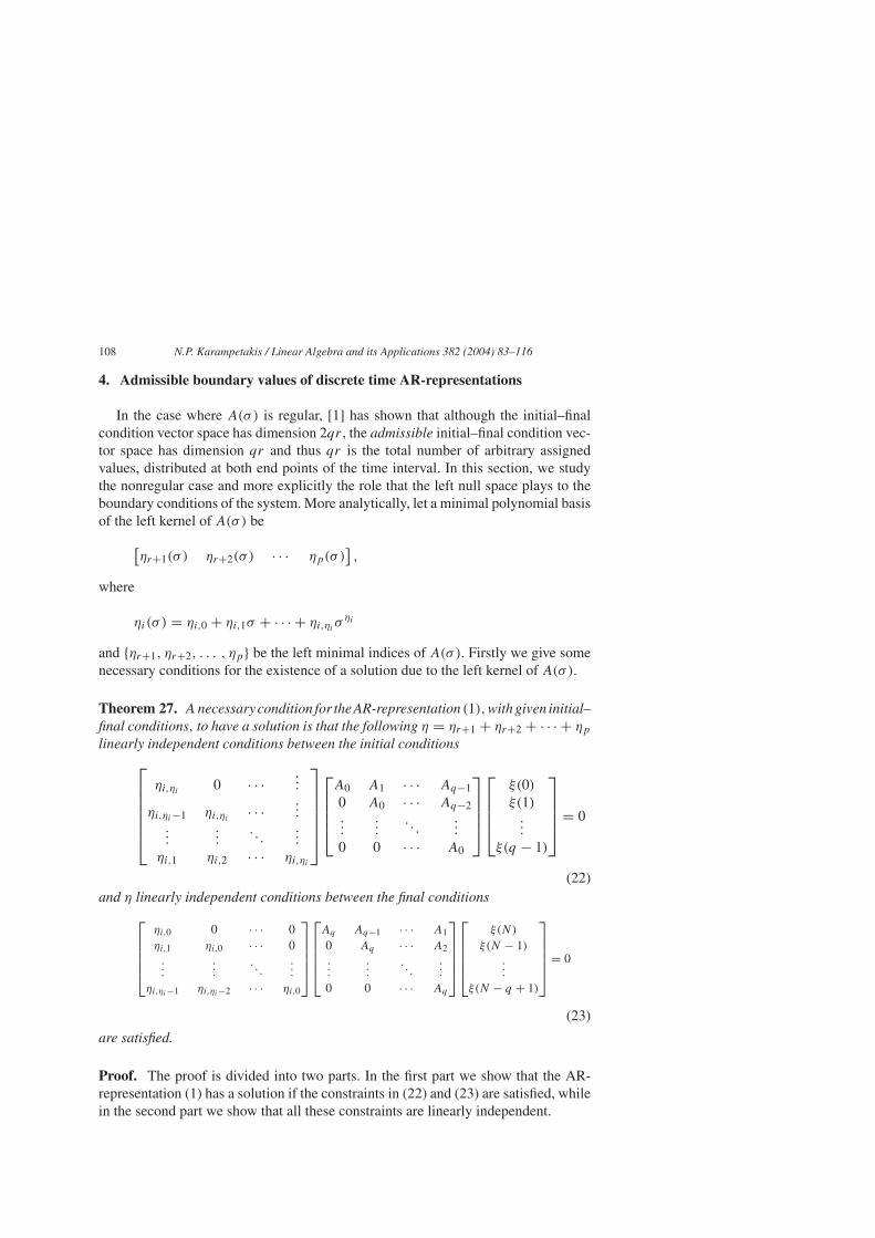
Theorem 27. A necessary condition for the AR-representation (1),with given initial–final conditions, to have a solution is that the following η = ηr+1 + ηr+2 + · · · + ηplinearly independent conditions between the initial conditions
ηi,ηi 0 · · · ...
ηi,ηi−1 ηi,ηi · · · ......
.... . .
...
ηi,1 ηi,2 · · · ηi,ηi
A0 A1 · · · Aq−10 A0 · · · Aq−2...
.... . .
...
0 0 · · · A0
ξ(0)ξ(1)...
ξ(q − 1)
= 0
(22)and η linearly independent conditions between the final conditions
ηi,0 0 · · · 0ηi,1 ηi,0 · · · 0...
.
.
.. . .
.
.
.
ηi,ηi−1 ηi,ηi−2 · · · ηi,0
Aq Aq−1 · · · A1
0 Aq · · · A2...
.
.
.. . .
.
.
.
0 0 · · · Aq
ξ(N)
ξ(N − 1)...
ξ(N − q + 1)
= 0
(23)
are satisfied.
Proof. The proof is divided into two parts. In the first part we show that the AR-representation (1) has a solution if the constraints in (22) and (23) are satisfied, whilein the second part we show that all these constraints are linearly independent.

N.P. Karampetakis / Linear Algebra and its Applications 382 (2004) 83–116 109
(a) It is easily seen from (4) that a necessary and sufficient condition so that thesystem (1) would have a solution is the following:
rankR(z)[A(z) | Zq�q ξ (0)+ ZN�0ξ (N)
]= rankR(z)[A(z)]. (24)
The geometrical meaning of the condition (24) is that the space W which is spannedby the columns of A(z) is exactly the same as the space Z which is spanned bythe columns of A(z) and the initial value vector Zq�q ξ (0)+ ZN�0ξ (N). An
equivalent condition is that their orthogonal spaces WT and ZT respectively are thesame. Thus if
ηi(z) := ηi,0 + ηi,1z+ · · · + ηi,ηi zηi ∈ R[z]1×p
is a polynomial vector of the left kernel of A(z), then by premultiplying both sidesof (4) with ηi(z) ∈ R[z]1×p we obtain that
ηi(z)A(z)ξ(z)
= [ηi,0 + ηi,1z+ · · · + ηi,ηi z
ηi] [zqIp · · · zIp Ip
]
×
Aq 0 · · · 0Aq−1 Aq · · · 0...
.... . .
...
A1 A2 · · · Aq
ξ(0)ξ(1)...
ξ(q − 1)
+ [ηi,0 + ηi,1z+ · · · + ηi,ηi z
ηi] [z−NIp · · · z−N+q−2Ip z−N+q−1Ip
]
×
A0 0 · · · 0A1 A0 · · · 0...
.... . .
...
Aq−1 Aq−2 · · · A0
ξ(N)
ξ(N − 1)...
ξ(N − q + 1)
.
We can easily see that the left part of the above equation is zero. Taking into accountthat −N + q − 1 + max{ηi} < 0 �⇒ N > q − 1 + max{ηi}, we get[
ηi,0 + ηi,1z+ · · · + ηi,ηi zηi] [zqIp · · · z2Ip zIp
]
×
Aq 0 · · · 0Aq−1 Aq · · · 0...
.
.
.. . .
.
.
.
A1 A2 · · · Aq
ξ(0)ξ(1)...
ξ(q − 1)
= [ηi,0z
q + ηi,1zq+1 + · · · + ηi,ηi z
ηi+q · · · ηi,0z+ ηi,1z2 + · · · + ηi,ηi z
ηi+1]
×
Aq 0 · · · 0Aq−1 Aq · · · 0...
.
.
.. . .
.
.
.
A1 A2 · · · Aq
ξ(0)ξ(1)...
ξ(q − 1)

110 N.P. Karampetakis / Linear Algebra and its Applications 382 (2004) 83–116
= − [zηi Ip · · · z2Ip zIp
]ηi,ηi 0 · · ·
.
.
.
ηi,ηi−1 ηi,ηi · · ·...
.
.
....
. . ....
ηi,1 ηi,2 · · · ηi,ηi
×
A0 A1 · · · Aq−1
0 A0 · · · Aq−2...
.
.
.. . .
.
.
.
0 0 · · · A0
ξ(0)ξ(1)...
ξ(q − 1)
.
Similarly
[ηi,0 + ηi,1z+ · · · + ηi,ηi z
ηi] [z−NIp · · · z−N+q−2Ip z−N+q−1Ip
]
×
A0 0 · · · 0A1 A0 · · · 0...
.
.
.. . .
.
.
.
Aq−1 Aq−2 · · · A0
ξ(N)
ξ(N − 1)...
ξ(N − q + 1)
= [ηi,0z
−N + ηi,1z−N+1 + · · · + ηi,ηi z
−N+ηi · · ·ηi,0z
−N+q−1 + ηi,1z−N+q + · · · + ηi,ηi z
−N+q−1+ηi ]
×
A0 0 · · · 0A1 A0 · · · 0...
.
.
.. . .
.
.
.
Aq−1 Aq−2 · · · A0
ξ(N)
ξ(N − 1)...
ξ(N − q + 1)
= [z−N z−N+1 · · · z−N+q−1+ηi ]
ηi,0 0 · · · 0ηi,1 ηi,0 · · · 0...
.
.
.. . .
.
.
.
ηi,ηi ηi,ηi−1 · · ·...
0 ηi,ηi · · ·...
.
.
....
. . ....
0 0 · · · ηi,ηi
×
A0 0 · · · 0A1 A0 · · · 0...
.
.
.. . .
.
.
.
Aq−1 Aq−2 · · · A0
ξ(N)
ξ(N − 1)...
ξ(N − q + 1)

N.P. Karampetakis / Linear Algebra and its Applications 382 (2004) 83–116 111
= − [z−N z−N+1 · · · z−N+q−1+ηi ]
0 0 · · · 00 0 · · · 0...
.
.
.. . .
.
.
.
ηi,0 0 · · ·...
ηi,1 ηi,0 · · ·...
.
.
....
. . ....
ηi,ηi−1 ηi,ηi−2 · · · ηi,0
×
Aq Aq−1 · · · A1
0 Aq · · · A2...
.
.
.. . .
.
.
.
0 0 · · · Aq
ξ(N)
ξ(N − 1)...
ξ(N − q + 1)
= − [z−N+q−1 z−N+q · · · z−N+q−1+ηi ]
ηi,0 0 · · · 0ηi,1 ηi,0 · · · 0...
.
.
.. . .
.
.
.
ηi,ηi−1 ηi,ηi−2 · · · ηi,0
×
Aq Aq−1 · · · A1
0 Aq · · · A2...
.
.
.. . .
.
.
.
0 0 · · · Aq
ξ(N)
ξ(N − 1)...
ξ(N − q + 1)
.
Equating the powers of z to zero we get the necessary boundary conditions of thetheorem.
(b) Following similar lines to the ones in [7] and with the help of the next corol-lary, we prove that the above conditions are linearly independent. �
Corollary 28. Note that the condition (23) between the final conditions may berewritten as follows:
ηi,0 0 · · · 0ηi,1 ηi,0 · · · 0...
.
.
.. . .
.
.
.
ηi,ηi−1 ηi,ηi−2 · · · ηi,0
Aq Aq−1 · · · A1
0 Aq · · · A2...
.
.
.. . .
.
.
.
0 0 · · · Aq
ξ(N)
ξ(N − 1)...
ξ(N − q + 1)
= 0
⇔
ηi,0 0 · · · 0ηi,1 ηi,0 · · · 0...
.
.
.. . .
.
.
.
ηi,ηi−1 ηi,ηi−2 · · · ηi,0
A1 A2 · · · Aq
A2 A3 · · · 0...
.
.
.. . .
.
.
.
Aq 0 · · · 0
ξ(N − q + 1)ξ(N − q + 2)
.
.
.
ξ(N)
= 0
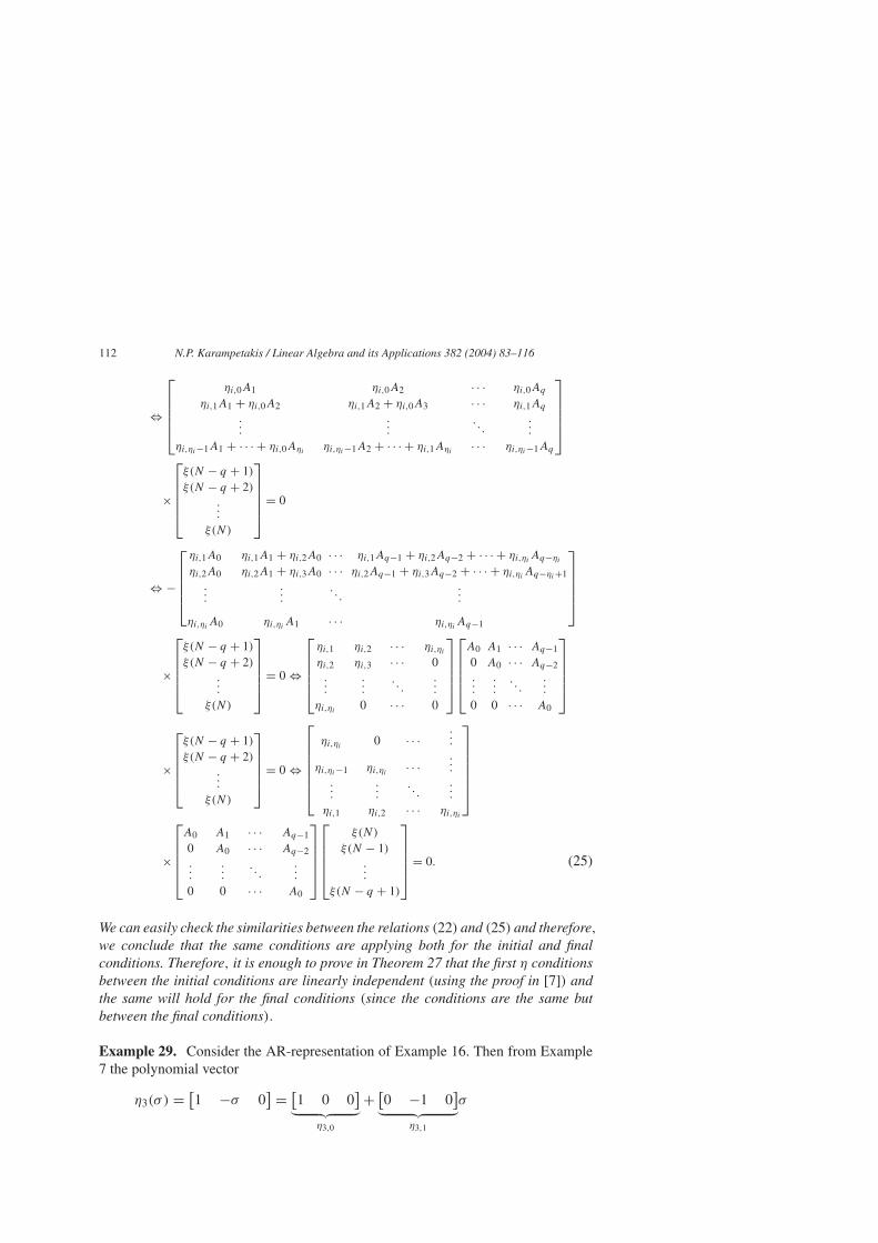
112 N.P. Karampetakis / Linear Algebra and its Applications 382 (2004) 83–116
⇔
ηi,0A1 ηi,0A2 · · · ηi,0Aq
ηi,1A1 + ηi,0A2 ηi,1A2 + ηi,0A3 · · · ηi,1Aq...
.
.
.. . .
.
.
.
ηi,ηi−1A1 + · · · + ηi,0Aηi ηi,ηi−1A2 + · · · + ηi,1Aηi · · · ηi,ηi−1Aq
×
ξ(N − q + 1)ξ(N − q + 2)
.
.
.
ξ(N)
= 0
⇔ −
ηi,1A0 ηi,1A1 + ηi,2A0 · · · ηi,1Aq−1 + ηi,2Aq−2 + · · · + ηi,ηi Aq−ηiηi,2A0 ηi,2A1 + ηi,3A0 · · · ηi,2Aq−1 + ηi,3Aq−2 + · · · + ηi,ηi Aq−ηi+1...
.
.
.. . .
.
.
.
ηi,ηi A0 ηi,ηi A1 · · · ηi,ηi Aq−1
×
ξ(N − q + 1)ξ(N − q + 2)
.
.
.
ξ(N)
= 0 ⇔
ηi,1 ηi,2 · · · ηi,ηiηi,2 ηi,3 · · · 0...
.
.
.. . .
.
.
.
ηi,ηi 0 · · · 0
A0 A1 · · · Aq−1
0 A0 · · · Aq−2...
.
.
.. . .
.
.
.
0 0 · · · A0
×
ξ(N − q + 1)ξ(N − q + 2)
.
.
.
ξ(N)
= 0 ⇔
ηi,ηi 0 · · ·
.
.
.
ηi,ηi−1 ηi,ηi · · ·...
.
.
....
. . ....
ηi,1 ηi,2 · · · ηi,ηi
×
A0 A1 · · · Aq−1
0 A0 · · · Aq−2...
.
.
.. . .
.
.
.
0 0 · · · A0
ξ(N)
ξ(N − 1)...
ξ(N − q + 1)
= 0. (25)
We can easily check the similarities between the relations (22) and (25) and therefore,we conclude that the same conditions are applying both for the initial and finalconditions. Therefore, it is enough to prove in Theorem 27 that the first η conditionsbetween the initial conditions are linearly independent (using the proof in [7]) andthe same will hold for the final conditions (since the conditions are the same butbetween the final conditions).
Example 29. Consider the AR-representation of Example 16. Then from Example7 the polynomial vector
η3(σ ) = [1 −σ 0
] = [1 0 0
]︸ ︷︷ ︸η3,0
+ [0 −1 0
]︸ ︷︷ ︸η3,1
σ

N.P. Karampetakis / Linear Algebra and its Applications 382 (2004) 83–116 113
constitutes a polynomial basis of the left kernel of A(σ). The AR-representation,according to the above theorem, must satisfy the following 2η = 2η3 = 2 conditionsbetween the initial–final conditions:
[η3,1 0 0 0
]A0 A1 A2 A30 A0 A1 A20 0 A0 A10 0 0 A0
ξ (0)ξ (1)ξ (2)ξ (3)
= 0
⇔ η3,1A0ξ (0)+ η3,1A1ξ (1)+ η3,1A2ξ (2)+ η3,1A3ξ (3) = 0
⇔ [0 −1 0
]0 0 01 0 10 1 0
ξ1 (0)ξ2 (0)ξ3 (0)
+ [
0 −1 0]1 0 1
0 0 10 1 0
×ξ1 (1)ξ2 (1)ξ3 (1)
+ [
0 −1 0]0 0 1
0 0 00 0 0
ξ1 (2)ξ2 (2)ξ3 (2)
+ [
0 −1 0]
×0 0 0
0 1 00 0 0
ξ1 (3)ξ2 (3)ξ3 (3)
= 0
⇔ −ξ1 (0)− ξ3 (0)− ξ3 (1)− ξ2 (3) = 0
[η3,0 0 0 0
]A4 A3 A2 A10 A4 A3 A20 0 A4 A30 0 0 A4
ξ (N)
ξ (N − 1)ξ (N − 2)ξ (N − 3)
= 0
⇔ η3,0A4ξ (N)+ η3,0A3ξ (N − 1)+ η3,0A2ξ (N − 2)+ η3,0A1ξ (N − 3) = 0
⇔ [1 0 0
]0 1 00 0 00 0 0
ξ1 (N)
ξ2 (N)
ξ3 (N)
+ [1 0 0
]0 0 00 1 00 0 0
ξ1 (N − 1)ξ2 (N − 1)ξ3 (N − 1)
+ [1 0 0
]0 0 10 0 00 0 0
ξ1 (N − 2)ξ2 (N − 2)ξ3 (N − 2)
+ [1 0 0
]1 0 10 0 10 1 0
ξ1 (N − 3)ξ2 (N − 3)ξ3 (N − 3)
= 0
⇔ ξ2 (N)+ ξ3 (N − 2)+ ξ1 (N − 3)+ ξ3 (N − 3) = 0.
We have shown in (21), that every solution ξ(k), k = 0, 1, . . . , n of (1) is givenby

114 N.P. Karampetakis / Linear Algebra and its Applications 382 (2004) 83–116
ξ(k) := [CF CB
] [J kF 00 JN−k
B
] [ζFζB
]+ x(k)
for k = 0, 1, . . . , N, for a specific vector ζ = [ζTF ζT
B ]T ∈ R(n+µ+2ε). The pro-posed solution ξ(k)must satisfy also the initial–final conditions. The initial conditionvector is given by
ξ(0)ξ(1)...
ξ(q − 1)
︸ ︷︷ ︸ξ (0)
=
CF CBJNB
CFJF CBJN−1B
......
CF Jq−1F CBJ
N−q+1B
︸ ︷︷ ︸Q0
[ζFζB
]+
x(0)x(1)...
x(q − 1)
︸ ︷︷ ︸x(0)
,
where x(0) ∈ Kernel[�q ]while the final condition vector is given by
ξ(N)
ξ(N − 1)...
ξ(N − q + 1)
︸ ︷︷ ︸ξ (N)
=
CFJNF CB
CFJN−1F CBJB...
...
CF JN−q+1F CBJ
q−1B
︸ ︷︷ ︸Q1
[ζFζB
]+
x(N)
x(N − 1)...
x(N − q + 1)
︸ ︷︷ ︸x(N)
,
where x(N) ∈ Kernel[�0].Combining the above two relations we get[
ξ (0)ξ (N)
]=
[Q0 00 Q1
] [ζFζB
]+
[x(0)x(N)
]. (26)
Therefore, (22), (25) and (26) provide us with necessary and sufficient conditions inorder for the AR-representation (1) to have a solution. Moreover, we can easily provethat the matrix Q = [QT
0 QT1 ]T ∈ R2qm×(n+µ+2ε) has full column rank (based on
the fact that the solutions ξ(k) defined by the spectral pairs
{[CF CB ],
[JFJB
]}are
linearly independent, and following similar reasoning to the ones in [6] or by takinglarge enough N − q + 1 > µ+ ε). Therefore, the vector space
V0 =v =
[ξ (0)ξ (N)
]−
[x(0)x(N)
]∈ Im
([Q0 00 Q1
])ξ (0), ξ (N) satisfying (22), (25)
:= 40 ⊕X0
with X0 ={[
x(0)x(N)
], x(0) ∈ Kernel[�q ], x(N) ∈ Kernel[�0]
}

N.P. Karampetakis / Linear Algebra and its Applications 382 (2004) 83–116 115
has dimension equal to
dimV0 = 2qm− (n+ µ+ 2ε) = 2q(m− r)+ 2qr − (n+ µ+ 2ε) =Lemma 6= 2{q(m− r)− ε} + n+ µ+ 2ε + 2η
We can easily prove, according to Theorem 16, that
dimX0 = 2{q(m− r)− ε}and therefore, the possible dimension of40 is n+ µ+ 2ε + 2η. Taking into accountTheorem 27, 2η linearly independent conditions must be satisfied among the vectorsof 40 and thus
dim40 = n+ µ+ 2ε.
Therefore, the initial–final condition vectors are chosen from the n+ µ+ 2ε−dimensional vector space 40 modulo the space X0 or otherwise both the
initial–final condition vector[ξ (0)T ξ (N)T
]T ∈ 40 and[ξ (0)T ξ (N)T
]T ⊕[x(0)T x(N)T
]T ∈ 40 ⊕X0 gives rise to the same solution class. The connection
between dim40 and dim BD is obvious.
5. Conclusions
In this paper we have studied the solution vector space of discrete time nonregularAR-representations over a finite time interval and, thus, extending the results presen-ted in [1,6]. More specifically, we have shown that the solution space of discrete timenonregular AR-representations over a finite time interval is divided into equivalenceclasses, where each equivalence class represents the whole number of solutions ofthe AR-representation under certain boundary values (initial–final conditions). Thedimension of the new equivalence class space has been determined and is shownto be equal to the sum of the degrees of the finite and infinite elementary divisorsplus two times the sum of the right minimal indices (order accounted for) of thepolynomial matrix that describes the AR-representation. An algorithm for the con-struction of the forward and backward solution space of a nonregular discrete timeAR-representations over a finite time interval is given in terms of the structuralinvariants of the polynomial matrix which describe the system. Finally, we haveshown that the left kernel of the polynomial matrix which describes the systemplays a crucial role in the existence of solution on the boundary condition problem.The meaning of the algebraic structure of a polynomial matrix in relation to thesolution vector space of nonregular discrete time AR-representations has thus beenelucidated.

116 N.P. Karampetakis / Linear Algebra and its Applications 382 (2004) 83–116
The investigation of the solution vector space of discrete nonregular AR-represen-tations gives rise to numerous applications, such as the solution of the zeroing-outputproblem, the determination of the controllable or uncontrollable and observable orunobservable subspaces of discrete polynomial matrix descriptions etc.
Acknowledgements
I would like to thank the anonymous reviewer for reading the manuscript carefullyand for making valuable suggestions.
References
[1] E.N. Antoniou, A.I.G. Vardulakis, N.P. Karampetakis, A spectral characterization of the behavior ofdiscrete time AR-representations over a finite time interval, Kybernetika 34 (5) (1998) 555–564.
[2] T.G.J. Beelen, New algorithms for computing the Kronecker structure of a pencil with applicationsto systems and control theory, Ph.D. thesis, Technische Universiteit Eindhven, 1987.
[3] R.R. Bitmead, S.-Y. Kung, B.D.O. Anderson, T. Kailath, Greatest common divisors via generalizedSylvester and Bezout matrices, IEEE Trans. Automatic Control 23 (6) (1978) 1043–1047.
[4] G.D. Forney, Minimal bases of rational vector spaces with applications to multivariable linearsystem, SIAM J. Control 13 (1975) 493–520.
[5] H. Freeman, Discrete Time Systems: An Introduction to the Theory, Wiley, 1965.[6] I. Gogberg, P. Lancaster, L. Rodman, Matrix Polynomials, Academic Press, 1982.[7] N.P. Karampetakis, Notions of equivalence for linear time invariant multivariable systems, Depart-
ment of Mathematics, Aristotle University of Thessaloniki, Greece, 1993.[8] C. Praagman, Invariants of polynomial matrices, in: 1st European Control Conference, 1991, pp.
1274–1277.[9] A.I.G. Vardulakis, Linear Multivariable Control: Algebraic Analysis, and Synthesis Methods, John
Wiley and Sons, 1991.[10] J.C. Willems, From time series to linear systems: Part I. Finite dimensional linear time invariant
systems, Automatica 22 (5) (1986) 561–580.[11] J.C. Willems, Paradigms and puzzles in the theory of dynamical systems, IEEE Trans. Automatic
Control 36 (3) (1991) 259–294.