Embed Size (px)
Citation preview
Chapter 6
Episode II
On the Smith–Ewart Equations and RAFT/Emulsion
A mathematician is a machine for converting coffee into theorems.
– Alfréd Rényi (1921−1970)
Chapter 6 On the Smith–Ewart Equations and RAFT/Emulsion
126
6.1 Kinetics of Particle Growth
It was established in Chapter 5 that c and kpCp are of similar magnitude in many RAFT-
containing systems and that zero-one kinetics therefore become inapplicable (see also
Chapter 4); therefore, it is either pseudo-bulk kinetics are applicable or, alternatively, the
kinetics may be described by neither the pseudo-bulk nor zero-one limits. In Chapter 4,
an overview of the zero-one and pseudo-bulk limits for the kinetics of particle growth
was given, showing that, in the case where (ρ/c ≈ 1 or k/c ≈ 1) and (ρ/c v 1 and k/c v 1),
the kinetics are not well-described by either of these limits. Moreover, it will be shown in
Chapter 7 that all three of the Smith–Ewart parameters (ρ, k and c) are of similar
magnitude. Thus, it is necessary to consider particle growth kinetics more closely.
In dealing with the exit of radicals from particles, their fate in the aqueous-phase
and the additional entry and termination processes, it is instructive to examine the roots of
both the zero-one and pseudo-bulk limits. The common roots for these kinetic schemes
are the seemingly simple Smith–Ewart equations.
6.2 The Smith–Ewart Equations
In an emulsion polymerization in which particle formation does not occur and termination
is chain-length independent, the population of particles with i radicals, Ni, is determined
by the rate coefficients for the processes that change the number of radicals in a particle
and the initial conditions of the system. In particular, intra-particle termination is
described by the pseudo-first-order rate coefficient for the destruction of two radicals, c,
radical entry by a first-order rate coefficient, ρ, and the loss of a single radical from a
particle by the first-order rate coefficient, k. Physical processes that may correspond to ρ,
k and c are the entry of an aqueous phase radical into a particle (ρ), the desorption of a
monomeric radical formed by a transfer to monomer reaction (k) and termination (c).
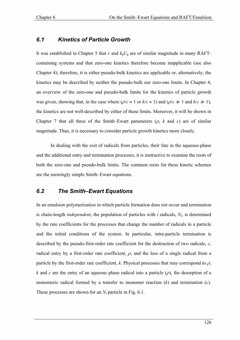
These processes are shown for an Ni particle in Fig. 6.1.
Chapter 6 On the Smith–Ewart Equations and RAFT/Emulsion
127
Ni+2
Ni+1
Ni
Ni−1
Ni−2
ρ
ρ
k
k
c
c
Figure 6.1: A schematic of the events changing the number of radicals in the particles containing i radicals.
The processes shown in Fig. 6.1 may be reduced to a time-evolution equation for
the population of Ni-type particles, the infinite set of which comprise the Smith–Ewart
equations:1
dNidt = ρ[ ]Ni−1 − Ni + k[ ](i + 1)Ni+1 − iNi + c[ ](i + 2)(i + 1)Ni+2 − i(i − 1)Ni
(6.1)
Note that, since a particle with i radicals in it may have any one of the i radicals exit
(through whatever mechanism is involved in that exit), the rate coefficient for exit per
particle (as opposed to per radical) is also proportional to i; similarly, the rate coefficient
for termination per particle is proportional to i(i − 1).
While these equations provide insight into the population balances of radicals in
the particles and their importance should not be underestimated, they provide no direct
means of understanding the kinetics of the system. The work of Hawkett et al.2 provided
a suitable means of solving these equations using eigenvectors. The zero-one limit
emerged from the Smith–Ewart equations by truncating the infinite series of equations in
such a way that if a radical entered an N1 particle, pseudo-instantaneous termination
would result not in an N2 particle but in an N0 particle.3 An alternate closure relation was
found by Ballard et al.,4 assuming that n2–– − n– = n–2 (the case if the Ni follow a Poisson
distribution5), leading to pseudo-bulk kinetics.
Chapter 6 On the Smith–Ewart Equations and RAFT/Emulsion
128
It is recognized that the treatment of emulsion polymerization kinetics in terms of
the Smith–Ewart equations is a simplification that removes the chain-length dependence
of the termination reaction. Deviations from the Smith–Ewart equations have been
observed,6,7 and in general the chain-length dependence of termination cannot be ignored.
However, as will be discussed in Section 6.2.2, under certain circumstances the Smith–
Ewart equations are applicable; moreover, some of the conclusions based on a chain-
length independent treatment should be semi-quantitatively applicable to systems where
this chain-length independence assumption is inadmissible.
Consideration of the Smith–Ewart equations and the origins of the zero-one and
pseudo-bulk limits is a necessary step in developing a simplified model for
RAFT/emulsion systems. In Section 6.3, a method whereby average Smith–Ewart
parameters may be calculated from the full chain-length dependent kinetics is presented.
6.2.1 Exited Radicals and the Smith–Ewart Equations
Incorporating the fate of the exited radicals into the original Smith–Ewart equations
(Eq. 6.1) can often be done trivially by rewriting the Smith–Ewart equations in terms of
ρt (where the subscript denotes “total) instead of ρ. A fate parameter α ∈ [−1,1] may then
be introduced, making ρt a function of the true, initiator derived radical flux ρ and the
average number of radicals per particle, n–:4,8
ρt = ρ + αkn– (6.2)
However, the use of the fate parameter is problematic in that, for fates other than the
limiting cases of α ∈ {−1, 0, 1}, α itself is a function of n–. For this reason, the treatment
here will be confined to a brief overview of the use of α when it falls into one of these
limits; other cases require the full treatment of the aqueous-phase kinetics to estimate the
fate of the exited radicals in the aqueous phase.

Chapter 6 On the Smith–Ewart Equations and RAFT/Emulsion
129
The fate of the exited radicals in zero-one kinetics gives five separate limits
depending on the efficiency of the initiator, whether or not complete aqueous-phase
termination occurs and whether a re-entering radical will stay in a particle that it re-enters
or desorb once more.5,9 The limiting values of α (i.e. −1, 0, 1) correspond to the following
fates (showing the exited radical as E ), which in the case of zero-one kinetics have been
ascribed names as shown:5,9
• α = +1:
o complete re-entry (and no subsequent re-escape) of the exited species
(Limit 2a).
• α = 0:
o complete aqueous-phase homotermination (e.g. E + E ) of the exited species
(Limit 1a), or
o complete aqueous-phase termination (e.g. E + IMi or E + E ) with an
initiator of low efficiency (Limit 1c), or
o continual re-entry and re-escape of the exited species until termination in a
particle (e.g. E + P ) occurs (Limit 2b).
• α = −1:
o complete aqueous-phase heterotermination (e.g. E + IMi ) of the exited
species with an initiator of otherwise high-efficiency (Limit 1b).
While there is great aesthetic appeal in using the fate parameter α, there are
difficulties in its application. In addition to α itself being a function of n– except in the
limiting cases above, ρt may now be a function of n–, making the differential equations
considerably more difficult to solve. Given these difficulties with the use of α, it will not
be used in this work except for the purposes of mathematical convenience and to
highlight the particular form of Eq. 6.2 being used.
Chapter 6 On the Smith–Ewart Equations and RAFT/Emulsion
130
In an uncompartmentalized system, the complete re-entry of the exited species
(with no re-escape) is equivalent to α = 1 in Eq. 6.2; this approximation makes the system
somewhat easier to solve, giving the familiar pseudo-bulk equation:4
dn–
dt = ρ − 2cn–2 (6.3)
It must be noted that, for the purposes of clarity, the formulation here is slightly
different from that shown elsewhere. In particular, there is often confusion between
whether ρ is ρt or ρi (initiator-derived radicals), especially when considering conditions
such as ρ/c à 1. Here and in the subsequent treatment of the Smith–Ewart equations and
the zero-one and pseudo-bulk limits, ρ will always be used to represent only the entry of
initiator-derived radicals, with the re-entry of other radicals being denoted with alternate
subscripts where appropriate.
6.2.2 Full Treatment of Polymer Kinetics
The occurrence of desorption requires taking into account the fate of exited free radicals,
which can be implemented by extending the Smith–Ewart equations to differentiate
particles containing one or more monomeric radicals (which can desorb) from particles
containing the same number of longer radicals (which cannot desorb).9 It is also essential
to note that the Smith–Ewart equations do not take chain-length dependent (CLD)
termination into account; therefore, they are only semi-quantitative for all except zero-
one systems and systems where termination is independent of chain length (e.g. where
termination by reaction-diffusion is dominant).10
When the effects of CLD termination are taken into account, one can still apply
the Smith–Ewart equations, but in general all the rate coefficients (ρ, k and c) will not be
constant, but will depend on the instantaneous radical distribution and the number of
radicals in each particle.10 Explicitly, c is a function of the number of radicals in the
particle, i, and also of the overall instantaneous distributions of all the Gi(N) (chain-length
distributions of growing chains within that particle), the instantaneous distributions of all
Chapter 6 On the Smith–Ewart Equations and RAFT/Emulsion
131
the Di(N) (chain-length distributions of dormant chains within that particle) and ρ is a
function of the overall number of monomeric radicals within all particles. In general,
these dependencies can only be found by a solution of the more complete system where
explicit account is taken of the distributions of the lengths of each chain in each particle.
This forms an extremely complex set of hierarchical equations replacing Eq. 6.1:10
dNidt = ρ i−1(N)[ ]Ni−1 − Ni + k[ ](i + 1)Ni+1 − iNi
+ ci+2( )Gi+2(N), Di+2(N) [ ](i + 2)(i + 1)Ni+2 − ci( )Gi(N), Di(N) (i − 1)Ni (6.4)
In Section 6.3, a method is described whereby the “instantaneous” Smith–Ewart rate
coefficients can be determined from the full CLD kinetics for the direct interpretation of
experimental data.
6.2.3 Solution of the Smith–Ewart Equations
Along with the pseudo-bulk limit of the Smith–Ewart equations, Ballard et al.4 also
reported a simple method of finding approximate solutions to the full Smith–Ewart
equations (Eq. 6.1) using a recursive approach. A brief summary of this process is as
follows.
Ballard et al.4 made use of a physical limit of the Ni particles as their closure
relation:
limi→∞
Ni = 0 (6.5)
Thus, by selecting a sufficiently large i = n and setting all Ni = 0 for i > n, the infinite set
of equations described by Eq. 6.1 is reduced to a more manageable set of n equations. The
accuracy of this artificial truncation procedure was verified by Ballard et al.4 against
alternative solution methods presented by Stockmayer11 and O’Toole.12
Solving the truncated set of equations in steady state then yields the following set
of equations that are readily solved starting with Nn set to an arbitrary value. Strictly, the
Chapter 6 On the Smith–Ewart Equations and RAFT/Emulsion
132
value selected for Nn will determine the normalization of the population distribution but
this is readily renormalized after all calculations have been performed; however, care
must be taken to prevent numerical overflows in the computation of the other Ni.
Nn−1 = 1
ρ { }[ ]ρ + nk + n(n − 1)c Nn (6.6)
Nn−2 = 1
ρ { }[ ]ρ + (n − 1)k + (n − 1)(n − 2)c Nn−1 − [ ]ρ + nk Nn (6.7)
Ni = 1
ρ { }[ ]ρ + (i + 1)k + i(i + 1)c Ni+1 − (i + 2)kNi+2 − (i + 3)(i + 2)cNi+3 (6.8)
A minimum value of n required for a reasonable approximation for the population
distribution was estimated by Ballard et al.4 to be 5(n– + 1), where n– is estimated from the
steady-state solution of Eq. 6.3. (In the case of a zero-one system where the true value of
n– is around ½, the value of n so calculated is around 5, which is sufficient for the zero-one
system.)
It may be noted from Eq. 6.1 that the population distribution (and hence n–) is
dependent only on the values of ρ/c and k/c; these three parameters may thus be reduced
to two when considering the value of n– that describes a system. Repeating the above
process for the calculation of n– over a range of values of ρ/c and k/c produces a surface of
n– values that describes various systems, shown in Fig. 6.2. Note the plateau in the surface
caused by the highly compartmentalized systems that follow zero-one kinetics.
In the case where exiting radicals have some kinetic effect after exit (i.e. α ≠ 0 in
the vernacular of Eq. 6.2), their effect must also be incorporated into this solution
method. In the limiting cases where α itself is not a function of n– (i.e. −1, 1), this may be
done in a straightforward (albeit computationally inefficient) method by first preparing an
estimate for n– using Eq. 6.6 to 6.8 and the truncation method described above, then using
Eq. 6.2 to determine a new value of ρ to be used once more in Eq. 6.6 to 6.8.4 This
procedure may be repeated until the value of n– is of sufficient accuracy. In practice, this
technique converges quite quickly to the actual value of n–. In the case of complete
Chapter 6 On the Smith–Ewart Equations and RAFT/Emulsion
133
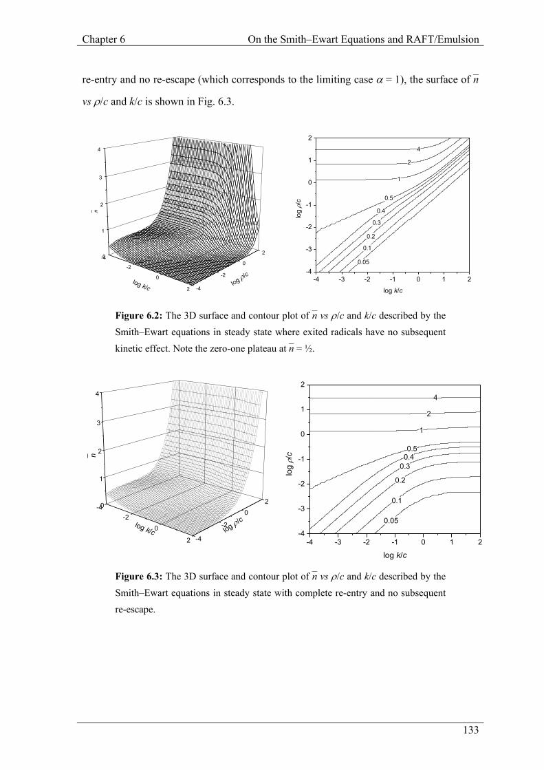
re-entry and no re-escape (which corresponds to the limiting case α = 1), the surface of n–
vs ρ/c and k/c is shown in Fig. 6.3.
-4
-2
0
2
0
1
2
3
4
-4
-2
0
2
_ n
log ρ/clog k/c
0.4
0.3
0.5
0.2
0.1
0.05
1
2
4
-4 -3 -2 -1 0 1 2-4
-3
-2
-1
0
1
2
log k/clo
g ρ/
c
Figure 6.2: The 3D surface and contour plot of n– vs ρ/c and k/c described by the Smith–Ewart equations in steady state where exited radicals have no subsequent kinetic effect. Note the zero-one plateau at n– = ½.
-4-2
0
2
0
1
2
3
4
-4
-2
02
_ n
log ρ/clog k/c
0.40.5
0.3
1
0.2
0.1
2
0.05
4
-4 -3 -2 -1 0 1 2-4
-3
-2
-1
0
1
2
log k/c
log
ρ/c
Figure 6.3: The 3D surface and contour plot of n– vs ρ/c and k/c described by the Smith–Ewart equations in steady state with complete re-entry and no subsequent re-escape.
Chapter 6 On the Smith–Ewart Equations and RAFT/Emulsion
134
6.2.4 Limits of the Smith–Ewart Equations
The applicability of the zero-one and pseudo-bulk limits to the Smith–Ewart equations
has already been discussed, with various conditions in terms of the relative magnitudes of
ρ, k and c being devised. In particular, it was noted that, in the case where (ρ/c ≈ 1 or
k/c ≈ 1) and (ρ/c v 1 and k/c v 1), neither of these limits would appear to hold.
However, it is possible that, while neither limit may be rigorously derived under such
conditions, the values for n– that result from one or other of these limits may still provide
useful approximations to the value of n–.
As it has previously been shown that the limit of complete re-entry and no
re-escape is suitable for the emulsion polymerization of styrene,5,13 the discussion
presented here will be restricted to this limit. It is noted that the treatment presented here
is for the steady state n– of the systems. The error in the value of n– calculated by the
various approximations to the Smith–Ewart equations presented here is, thus, only one
facet of these approximations; the accuracy of these limits in estimating the relaxation
kinetics and the molecular weight distributions is an area for further work outside the
scope of this study.
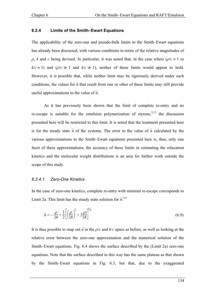
6.2.4.1 Zero-One Kinetics
In the case of zero-one kinetics, complete re-entry with minimal re-escape corresponds to
Limit 2a. This limit has the steady state solution for n–:5,9
n– = − ρ2k +
12
ρ
2k
2
+ 2ρ2k
½ (6.9)
It is thus possible to map out n– in the ρ/c and k/c space as before, as well as looking at the
relative error between the zero-one approximation and the numerical solution of the
Smith–Ewart equations. Fig. 6.4 shows the surface described by the (Limit 2a) zero-one
equations. Note that the surface described in this way has the same plateau as that shown
by the Smith–Ewart equations in Fig. 6.3, but that, due to the exaggerated
Chapter 6 On the Smith–Ewart Equations and RAFT/Emulsion
135
compartmentalization of the “zero-one” assumption, as ρ/c increases, the system remains
at n– = ½.
A contour-plot comparison of the relative error between the zero-one solution and
the numerical solution to the full Smith–Ewart equations presented above is shown in
Fig. 6.5. When ρ/c á 1 and k/c á 1, this error is quite small; however, when either
ρ/c à 1 or k/c à 1, this error becomes more substantial.
-4-3
-2-1
01
2
0.0
0.2
0.4
0.6
0.8
1.0
-4
-2
02
_ n
log ρ/clog k/c
0.400.30
0.20
0.49
0.100.05
-4 -3 -2 -1 0 1 2-4
-3
-2
-1
0
1
2
log k/c
log
ρ/c
Figure 6.4: The 3D surface and contour plot of n– vs ρ/c and k/c described by the zero-one equations with complete re-entry and minimal re-escape.
25 10
1520
30
50
75
-4 -2 0 2-4
-2
0
2
log k/c
log
ρ/c
Figure 6.5: Percentage error in the calculation of n– using zero-one kinetics as a function of ρ/c and k/c with complete re-entry and minimal re-escape.
Chapter 6 On the Smith–Ewart Equations and RAFT/Emulsion
136
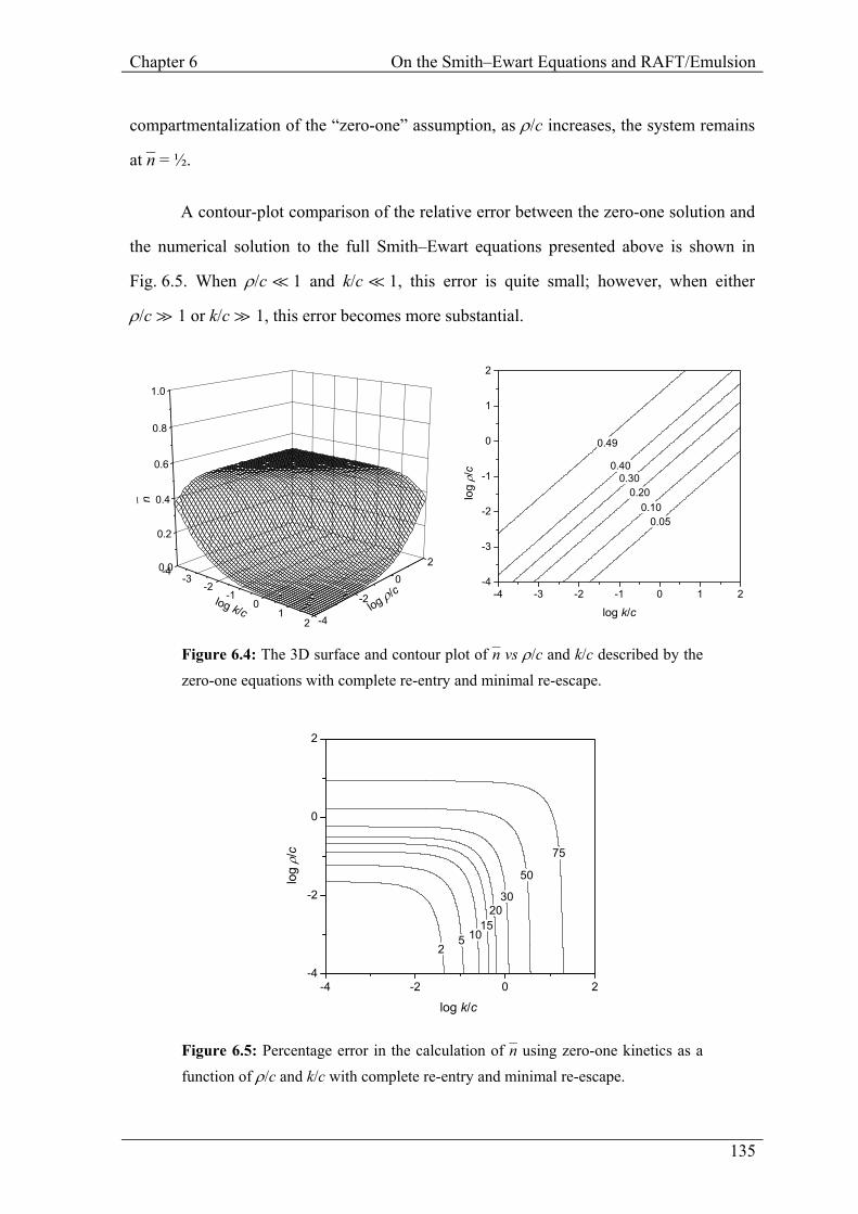
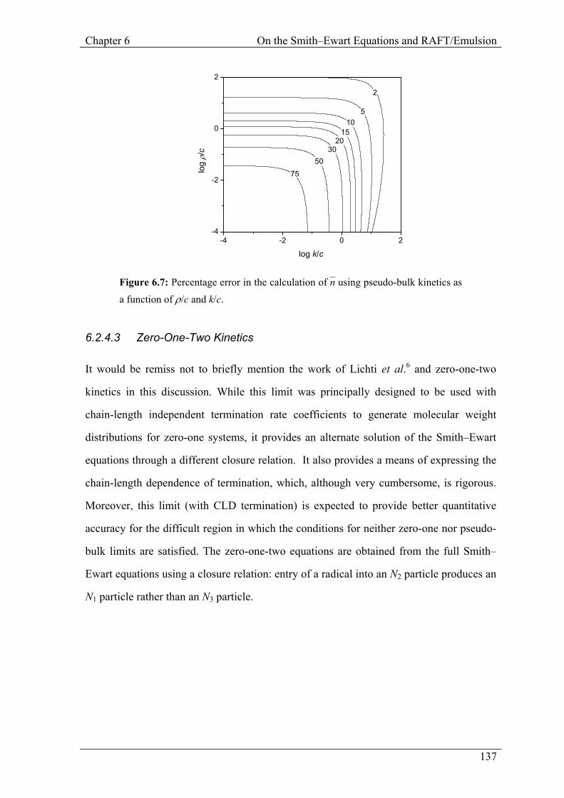
6.2.4.2 Pseudo-Bulk Kinetics
In the case of an uncompartmentalized system, complete re-entry and minimal
re-escape corresponds to pseudo-bulk kinetics.4 The differential equation describing the
time-evolution of n– (Eq. 6.3) has the steady state solution:
n– =
ρ
2c
½ (6.10)
Once more, it is possible to map out n– and the error in n– from pseudo-bulk calculations as
a function of ρ/c and k/c. These are shown in Fig. 6.6 and 6.7, showing that, for either
ρ/c à 1 or k/c à 1, the correspondence between the pseudo-bulk approximation and the
numerical solution to the Smith–Ewart equations is quite good.
-4-2
0
2
0
1
2
3
4
-4
-2
02
_ n
log ρ/clog k/c
0.05
0.1
0.20.30.4 0.5
1
2
4
-4 -3 -2 -1 0 1 2-4
-3
-2
-1
0
1
2
log k/c
log
ρ/c
Figure 6.6: The 3D surface and contour plot of n– vs ρ/c and k/c described by the pseudo-bulk equation.
Chapter 6 On the Smith–Ewart Equations and RAFT/Emulsion
137
7550
3020
1510
5
2
-4 -2 0 2-4
-2
0
2
log k/c
log
ρ/c
Figure 6.7: Percentage error in the calculation of n– using pseudo-bulk kinetics as a function of ρ/c and k/c.
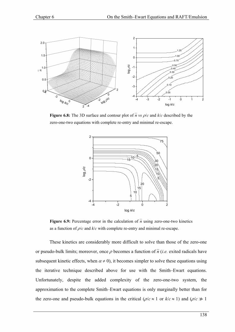
6.2.4.3 Zero-One-Two Kinetics
It would be remiss not to briefly mention the work of Lichti et al.6 and zero-one-two
kinetics in this discussion. While this limit was principally designed to be used with
chain-length independent termination rate coefficients to generate molecular weight
distributions for zero-one systems, it provides an alternate solution of the Smith–Ewart
equations through a different closure relation. It also provides a means of expressing the
chain-length dependence of termination, which, although very cumbersome, is rigorous.
Moreover, this limit (with CLD termination) is expected to provide better quantitative
accuracy for the difficult region in which the conditions for neither zero-one nor pseudo-
bulk limits are satisfied. The zero-one-two equations are obtained from the full Smith–
Ewart equations using a closure relation: entry of a radical into an N2 particle produces an
N1 particle rather than an N3 particle.
Chapter 6 On the Smith–Ewart Equations and RAFT/Emulsion
138
-4-2
0
2
0.0
0.5
1.0
1.5
2.0
-4
-2
02
_ n
log ρ/clog k/c
0.400.50
0.30
0.75
0.20
1.00
0.10
1.25
0.05
-4 -3 -2 -1 0 1 2-4
-3
-2
-1
0
1
2
log k/c
log
ρ/c
Figure 6.8: The 3D surface and contour plot of n– vs ρ/c and k/c described by the zero-one-two equations with complete re-entry and minimal re-escape.
510
15
1510 5
510
152030
50
20
75
-4 -2 0 2-4
-2
0
2
log k/c
log
ρ/c
Figure 6.9: Percentage error in the calculation of n– using zero-one-two kinetics as a function of ρ/c and k/c with complete re-entry and minimal re-escape.
These kinetics are considerably more difficult to solve than those of the zero-one
or pseudo-bulk limits; moreover, once ρ becomes a function of n– (i.e. exited radicals have
subsequent kinetic effects, when α ≠ 0), it becomes simpler to solve these equations using
the iterative technique described above for use with the Smith–Ewart equations.
Unfortunately, despite the added complexity of the zero-one-two system, the
approximation to the complete Smith–Ewart equations is only marginally better than for
the zero-one and pseudo-bulk equations in the critical (ρ/c ≈ 1 or k/c ≈ 1) and (ρ/c v 1
Chapter 6 On the Smith–Ewart Equations and RAFT/Emulsion
139
and k/c v 1) regions, as shown in Fig. 6.8 and 6.9. While it would appear that the use of
zero-one-two kinetics are unjustified in calculating steady-state values of n– with chain-
length independent termination, the zero-one-two model will be used as a basis for
calculating suitable average values of the pseudo-first-order rate coefficient for
termination in Section 6.3.
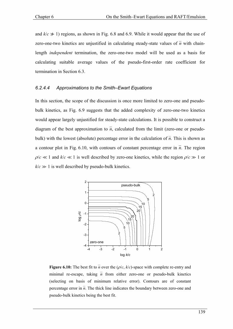
6.2.4.4 Approximations to the Smith–Ewart Equations
In this section, the scope of the discussion is once more limited to zero-one and pseudo-
bulk kinetics, as Fig. 6.9 suggests that the added complexity of zero-one-two kinetics
would appear largely unjustified for steady-state calculations. It is possible to construct a
diagram of the best approximation to n–, calculated from the limit (zero-one or pseudo-
bulk) with the lowest (absolute) percentage error in the calculation of n–. This is shown as
a contour plot in Fig. 6.10, with contours of constant percentage error in n–. The region
ρ/c á 1 and k/c á 1 is well described by zero-one kinetics, while the region ρ/c à 1 or
k/c à 1 is well described by pseudo-bulk kinetics.
2
510
1520
2015
105
2
-4 -3 -2 -1 0 1 2-4
-3
-2
-1
0
1
2pseudo-bulk
zero-one
log k/c
log
ρ/c
Figure 6.10: The best fit to n– over the (ρ/c, k/c)-space with complete re-entry and minimal re-escape, taking n– from either zero-one or pseudo-bulk kinetics (selecting on basis of minimum relative error). Contours are of constant percentage error in n–. The thick line indicates the boundary between zero-one and pseudo-bulk kinetics being the best fit.
Chapter 6 On the Smith–Ewart Equations and RAFT/Emulsion
140
The regions for which pseudo-bulk and zero-one kinetics are valid do not overlap.
Fig. 6.5 and 6.7 indicate that there is significant error (20−30%) in the region between
zero-one and pseudo-bulk kinetics. This is borne out in Fig. 6.10; the region where
(ρ/c ≈ 1 or k/c ≈ 1) and (ρ/c v 1 and k/c v 1) may be described by either zero-one or
pseudo-bulk kinetics only to an error of up to 30% in n–. Therefore, great care must be
taken in interpreting the modeling result of either zero-one or pseudo-bulk kinetics in this
region.
6.3 Chain-Length Dependence and Smith–Ewart Kinetics
The Smith–Ewart equations1 have been used to describe emulsion polymerization kinetics
in many systems, as they account for the compartmentalization of the radicals in the
system. In the formalism developed by Smith and Ewart,1 intra-particle termination is
described by the (average) chain-length independent, pseudo-first-order rate coefficient
for the destruction of two radicals, c. The treatment of emulsion polymerization kinetics
in terms of the Smith–Ewart equations is, thus, a simplification that removes the chain-
length dependence of the termination reaction.
Deviations from the Smith–Ewart equations due to CLD termination were
described by Lichti et al.6 and Adams et al.7 Ignoring the chain-length dependence of
termination is valid for zero-one systems and for pseudo-bulk systems at high weight-
fractions of polymer, wp, when the dominant termination mode becomes reaction-
diffusion termination, which is independent of chain length. As noted above, some of the
conclusions based on a chain-length independent treatment should be semi-quantitatively
applicable to systems where this chain-length independence assumption is inadmissible.
As noted earlier, the occurrence of desorption requires taking into account the fate
of exited free radicals, which can be implemented by extending these equations to
differentiate particles containing one or more monomeric radicals (which can desorb)
from particles containing the same number of longer radicals (which cannot desorb).9
Chapter 6 On the Smith–Ewart Equations and RAFT/Emulsion
141
When both CLD termination and radical desorption are taken into account, one
can still apply the Smith–Ewart equations, but in general all the rate coefficients (ρ, k and
c) will not be constant. Rather, they will depend on the instantaneous radical distribution
and on the number of radicals in each particle.10 Explicitly, c is a function of the number
of radicals in the particle, i, and also of the overall instantaneous distributions of all the
Gi(N) (chain-length distributions of growing chains within that particle) and ρ is a
function of the overall number of monomeric radicals within all particles. These
dependencies can in general only be found by a solution of the more complete system
where explicit account is taken of the distributions of the lengths of each chain in each
particle.10
Various limits and approximations to the Smith–Ewart equations have been
proposed, with the aim of variously describing the rate of polymerization or the molecular
weight distribution of the polymer formed. Commonly used limits have included the zero-
one limit3,5 (where entry of a radical into a particle already containing a growing radical
leads to pseudo-instantaneous termination) and the pseudo-bulk limit4 (where there is no
compartmentalization and the system polymerizes like the “equivalent” bulk system). The
zero-one-two model,14 where entry of a third radical into a particle leads to pseudo-
instantaneous termination, has also been used to account for the molecular weight
distributions.
In a compartmentalized system such as an emulsion polymerization, the effect of
CLD termination is difficult to include, with the generalized kinetic scheme resulting in
significant complexity. Even in the zero-one-two simplification with CLD termination,
the full expressions include coupled partial integrodifferential equations with three
independent variables (time and the length of the two radicals) that are generally
intractable.
The application of the Smith–Ewart equations to systems in which CLD
termination important is thus fraught with difficulties. Here, a method of taking account
Chapter 6 On the Smith–Ewart Equations and RAFT/Emulsion
142
of the chain-length dependence of termination will be demonstrated to generate
appropriate chain-length independent (average) parameters that may be used in the
Smith–Ewart equations. The method presented here will firstly be shown for the zero-
one-two limit14of the Smith–Ewart equations, with a generalization to systems containing
more radicals being subsequently presented.
6.3.1 Overall Strategy
In the case of zero-one-two kinetics, it is first shown that the rate of loss of particles with
two radicals in them (N2 particles) is determined by the time-dependent pseudo-first-order
rate coefficient for termination. Suitable physical models may be used to analytically
describe termination or alternate numerical methods implemented. Once the loss of N2
particles has been described, it is shown that this may be related to an average
termination rate coefficient that is applicable to the quasi-steady-state in which the
calculations were performed.
The notation used here is that of the distinguished particle equations of Lichti et
al.14 Here, the overall reaction time since the steady state was reached is denoted t, while
the time since the first (distinguished) radical entered the particle under consideration is
t′. The time for which two (distinguished) radicals have been in a particle is denoted t′′
and the proportion of particles that have two distinguished radicals in them is thus
N2′′(t, t′, t′′) or simply N2′′(t′′). The pseudo-first-order rate coefficient for termination
depends on the weight fraction of polymer in the system, wp(t), and the lengths of the two
radicals in the particle; it is thus written as c(t, t′, t′′) or simply c(t′′). The objective of the
derivations presented here is to offer methods for obtaining c–(t), the time-dependent rate
coefficient for termination averaged over the current population distribution of radicals to
account for CLD termination.
Chapter 6 On the Smith–Ewart Equations and RAFT/Emulsion
143
6.3.2 Average Termination Rate Coefficient in Zero-One-Two Kinetics
In a system where zero-one-two kinetics are applicable (e.g. ρ, k d c), the primary means
of loss of N2′′ particles is termination between the two radicals. The following relation is
thus found for the population balance N2′′(t′′):14
dN2′′(t′′)
dt′′ = − 2c(t′′)N2′′(t′′) (6.11)
Solution of this differential equation gives N2′′(t′′) as a function of c(t′′):
N2′′(t′′) = C1(t) exp( )−2 ∫ c(t′′) dt′′ (6.12)
where C1(t) is a constant of integration determined using the value of N2′′(0); N2′′(t′′) is a
monotonic decreasing function. Methods by which Eq. 6.12 may be solved are presented
in subsequent sections.
It will now be shown that this result for N2′′(t′′) may be related back to the zero-
one-two limit14 of the Smith–Ewart equations,1 where intra-particle termination is
described by the t-dependent pseudo-first-order rate coefficient for the destruction of two
radicals, c = c–(t), averaged over t′′ to account for CLD termination. Rewriting Eq. 6.11 in
terms of c–(t), one has:
dN2′′(t′′)
dt′′ = − 2c–(t)N2′′(t′′) (6.13)
where c–(t) is independent of t′′. This expression is integrated over t′′ from t′′ = 0 to the
limit as t′′ → ∞. Noting that the limit as t′′ → ∞ of N2′′(t′′) is 0 (eventually all radicals
must terminate), it is found that:
c–(t) = N2′′(0)
2 ⌡⌠0
∞
N2′′(t′′) dt′′ −1
(6.14)
To obtain values for c–(t), Eq. 6.12 must now be solved. In some cases, this may be
done analytically, as will be shown in the next section, while in other cases it is more
convenient to use numerical simulations to estimate this quantity.
Chapter 6 On the Smith–Ewart Equations and RAFT/Emulsion
144
6.3.2.1 Population Integral
It has been established experimentally15,16 and through theoretical arguments17 that the
rate coefficient for termination between an m-meric and n-meric radical, kmnt , is
determined by the mutual diffusion coefficient of the two radicals. In the case of the
termination of a long chain and a short chain, this diffusion coefficient is (to a good
approximation) that of the short chain, with the diffusion of the long chain making an
insignificant contribution to the mutual diffusion of the chain ends.17 If the short chain is
the m-meric chain, the termination rate coefficient, kmnt , may be written in terms of a
Smoluchowski diffusion reaction:17
kmnt ≈ 4πDmpmnσNA (6.15)
where Dm is the diffusion coefficient of the m-meric radical, pmn the probability of
reaction occurring during a collision (for radical-radical termination reactions, pmn = ¼
due to spin multiplicity, except at high conversion18,19) and σ is the interaction radius (for
styrene,20 σ ≈ 0.7 nm).
Since c(t′′) is the pseudo-first-order rate coefficient for termination per radical, it
may be written in terms of the concentration of m-meric radical in the particle, 1/NAVs,
where Vs is the swollen volume of the particle:
c(t′′) = kmnt (t′′)/NAVs (6.16)
Experimental studies of diffusion and termination have indicated that a power law
relationship between the diffusion coefficient and the length of the short chain may be
appropriate.16,21 One may then write:
Dm(wp) = D1(wp) m−β(wp) (6.17)
where D1(wp) is the diffusion coefficient of the monomer in the polymer matrix and β(wp)
is the scaling exponent. (It is noted that, in other work, α has been used as the exponent
Chapter 6 On the Smith–Ewart Equations and RAFT/Emulsion
145
for the chain-length dependence;22 for clarity, β is used here to differentiate from the fate
parameter described in Section 6.2.1.)
Both D1 and β are dependent on the weight fraction of polymer, wp, in the system,
with previous studies providing empirical relations for these quantities; in many cases
(such as in a γ-relaxation experiment), the dependence of D1 and β on wp can be neglected
as the experiment is conducted over a relatively narrow range of values of wp. Estimates
for D1 have been published for various monomers21,23 and expressions for β have been
found for systems below c*,16 and also well above c**.21
Following the notation of Lichti et al.,14 the length of the entering radical may be
expressed as a function of the time since entry, t′′. However, the length of the radical is
not simply proportional to t′′, as the radical already has a length z (where z is the critical
degree of polymerization for entry24) on entry. It is convenient to introduce a parameter
tz = z/(kpCp), giving the following expression for m:
m = [ ]t′′ + tz kpCp (6.18)
where kp is the second-order rate coefficient for propagation and Cp is the concentration
of monomer in the particle.
It is then possible to express c(t′′) as a function of Dm, noting that c(t′′) is also a
function of t due to the dependence on wp:
c(t′′) = c0(t) [ ]t′′ + tz−β(t) (6.19)
where
c0(t) = 4πpmnσ Vs−1D1(t)[ ]kpCp
−β(t) (6.20)
In considering the solution of Eq. 6.12 and then subsequently Eq. 6.14, it is
necessary to break the solution into different cases according to the value of β. Physically
reasonable values of β are [0,2], with β = 0 indicating no chain-length dependence and
Chapter 6 On the Smith–Ewart Equations and RAFT/Emulsion
146
β = 2 giving the reptation limit.25 In the cases detailed below where Eq. 6.14 is not
convergent, a more suitable model for c(t′′) must be chosen; in particular, once reaction
diffusion (where chain ends move by propagation) provides a significant contribution to
the diffusion of the radicals and when transfer to monomer is significant, the simple
scaling law of Eq. 6.19 is inapplicable.
Case 0 < β < 1:
Returning to Eq. 6.12, it is possible to analytically evaluate this expression given
the power law relation for c(t′′) shown in Eq. 6.19:
N2′′(t′′) = C1(t) N2′′(0) exp
−2c0(t)
1−β(t) [ ]t′′ + tz1−β(t) (6.21)
with C1(t) being evaluated using N2′′(0):
C1(t) = exp
2c0(t)
1−β(t) [ ]tz1−β(t) (6.22)
Evaluation of Eq. 6.14 is once again possible analytically, given the power law
dependence assumed here:
c–(t) = [ ]β(t)−1 [ ] 2c0(t)
1−β(t)
11−β(t)
2C1(t)Γ( )11−β(t) ,
2c0(t) tz1−α(t)
1−β(t)
(6.23)
where Γ(b, z) is the incomplete Γ-function:
Γ(b, z) = ⌡⌠z
∞
tb−1e−t dt (6.24)
Case β = 1:
The integral shown in Eq. 6.12 takes quite a different form when β = 1, giving:
N2′′(t′′) = C1(t) [ ]t′′ + tz−2c0(t) (6.25)
Chapter 6 On the Smith–Ewart Equations and RAFT/Emulsion
147
with C1(t) given by:
C1(t) = N2′′(0) [ ]tz−2c0(t) (6.26)
It is now possible to evaluate c–(t) using Eq. 6.14 in some circumstances,
depending on the value of c0(t). In the case where β = 1, Eq. 6.20 gives c0(t) ≈ c1L/kpCp,
where c1L is the pseudo-first-order rate coefficient for termination of the monomeric
radical under the short-long assumption used here. When c0(t) > ½, it is found that:
c–(t) = C1(t)
(2c0(t)−1)tz2c0(t)−1
(6.27)
However, for c0(t) < ½, the integral in Eq. 6.14 is divergent giving the unphysical result
c–(t) = 0. The value of c0(t) may cross the value of ½ during the course of a reaction: the
ratio between termination (i.e. diffusion) and propagation rate coefficients determines the
behavior of the system with c0 ∝ D1/(kpVs). Larger particles also tend to decrease c0(t) as
termination is less likely.
Case 1 < β < 2:
In the case where β > 1, N2′′(t′′) and C1(t) are given by Eq. 6.21 and 6.22; however, the
integral over all t′′ to find c(t′′) (Eq. 6.14) is divergent. In this case, it is not possible to
calculate c–(t) from a simple power law expression for c(t′′). The divergence of the
integral is unphysical, but easily understood given the assumptions of the model for
termination used here. Note also that the work of Griffiths et al.21 indicates that emulsion
polymerizations would normally have β > 1, making this shortcoming quite significant.
6.3.2.2 Population Integral with Reaction Diffusion and Transfer to Monomer
An alternate model for c(t′′) incorporating both reaction diffusion and chain transfer to
monomer permits the calculation of N2′′(t′′). With physically reasonable assumptions,
these two additions add equivalent complexity to the mathematics of the system; hence, it
is convenient to discuss them both together. However, the expression obtained for N2′′(t′′)
Chapter 6 On the Smith–Ewart Equations and RAFT/Emulsion
148
with either reaction-diffusion or transfer to monomer does not permit c–(t) to be obtained
analytically. Recourse to numerical methods is quite feasible in this case.
Incorporating reaction diffusion, the model for the diffusion of the terminating
radicals is as follows. The mutual diffusion coefficient may be constructed from the
center-of-mass diffusion coefficients for each species, Dcomm and Dcom
n , and the reaction-
diffusion coefficient for each chain, Drdm and Drd
n :20
Dmn = Dcomm + Dcom
n + Drdm + Drd
n (6.28)
As before, the center-of-mass diffusion coefficient for the longer n-meric species
may be neglected. Additionally, the reaction-diffusion term will be independent of chain-
length,20 giving:
Dm = Dcomm + 2Drd (6.29)
where Drd is given by:
Drd = kpCpa2/6 (6.30)
Here, a is the root-mean-square end-to-end distance per square root of the number
of monomer units in the polymer chain. Values for a for various monomers are given by
Russell et al.20
The rigorous inclusion of transfer to monomer is quite difficult. However, it was
shown by Clay et al.22 that the pseudo-first-order rate coefficient for transfer to monomer
was of similar magnitude to the pseudo-first-order average rate coefficient for
termination; moreover, approximately equal numbers of chains were stopped by transfer
and termination.22 One may conclude that the most probable fate for a monomeric radical
is termination with another radical, since the termination rate coefficient for a monomeric
radical is significantly greater than that of a longer chain, as noted in the experiments of
Adams et al.7 Working with this physically reasonable assumption that all monomeric
Chapter 6 On the Smith–Ewart Equations and RAFT/Emulsion
149
radicals terminate, a lower limit on the pseudo-first-order termination rate coefficient
c(t′′) is the transfer frequency, ktrCp.
Once again, using a power law relationship for the chain-length dependence of the
center-of-mass diffusion, an expression for c(t′′) may be obtained:
c(t′′) = c0(t) [ ]t′′ + tz−β(t) + crd + ctrM (6.31)
where c0(t) is defined as before (Eq. 6.20). The contribution of reaction-diffusion to
termination is crd(t) (pmn being dependent26 on wp and Cp being dependent on t):
crd(t) = 4πpmnσ kpCpa2
3Vs (6.32)
The contribution of transfer to monomer to termination, ctrM(t), is t-dependent as the
transfer reaction has been shown to have a dependence on wp at high conversion22,26 and
Cp varies throughout Interval III:
ctrM(t) = ktrCp (6.33)
As before, this expression may be integrated to give an expression for N2′′(t′′). For
example, in the case where β ≠ 1,
N2′′(t′′) = C1(t) exp
−2c0(t)
1−β(t) [ ]t′′ + tz1−β(t) − 2crdt′′ − 2ctrMt′′ (6.34)
with C1(t) being the same as defined in Eq. 6.22.
In general, it is not possible to integrate N2′′(t′′) as given in Eq. 6.34 over all t′′,
thus c–(t) cannot be obtained analytically from Eq. 6.19 and 6.34. However, numerical
computation of the integral over all N2′′(t′′) is relatively inexpensive, permitting this
method to be used to calculate a value of c–(t) that suitably takes account of the chain-
length dependence of termination in the Smith–Ewart equations.
Chapter 6 On the Smith–Ewart Equations and RAFT/Emulsion
150
6.3.2.3 Probabilistic Method
Analytic expressions for the probability that radicals will propagate j or more steps in a
two radical environment were used by Maeder and Gilbert27 to estimate the applicability
of zero-one kinetics to the polymerization of butyl acrylate. More recently, Monte Carlo
models were used by Prescott28 to estimate radical lifetimes in RAFT-mediated emulsion
polymerizations (although this technique could be equally well used with non-RAFT
systems). The inclusion of reaction-diffusion and transfer to monomer is quite simple in
these models, permitting the kinetics of the system to be more accurately modeled.
The probability that the two radicals in a particle will consume j or more monomer
units is denoted by Pj(t), noting that this will be a function of wp(t). It will first be shown
that the area under the Pj(t) vs j curves, constructed according to the method of Prescott28
(or alternatively Pj(t) vs 2j if using the method of Maeder and Gilbert27), provides a
measure of the average number of monomer units consumed before termination in a
particle, ∆m––(t), and that this, in turn, permits the evaluation of c–(t).
Consider a Pj(t) vs j curve generated by sequentially assessing N test-particles,
each originally containing 2 radicals. By definition, Pj(t) is the proportion of systems that
consumed j or more monomer units before a termination reaction occurred. Thus, NPj is
equal to the number of systems that consumed j or more monomer units and N(Pj − Pj+1)
is the number of systems that consumed precisely j monomer units. The (number) average
number of monomer units consumed in a system, ∆m––, is then given by:
∆m–– =
N(P1 − P2) + 2N(P2 − P3) + 3N(P3 − P4) + … N (6.35)
which simplifies to:
∆m–– = ∑
j ≥ 0Pj (6.36)
This may be reduced to an integral form through a discrete-to-continuous approximation
for j:
Chapter 6 On the Smith–Ewart Equations and RAFT/Emulsion
151
∆m–– = ⌡⌠
0
∞
Pj dj (6.37)
It will now be shown that ∆m––(t) may be related back to c–(t). The time taken for j
monomer units to be consumed in a particle with two radicals, t′′, is:
t′′ = j/2kpCp (6.38)
Changing the variable of integration in Eq. 6.37 from j to t′′ using Eq. 6.38 yields the
following integral over time for the number of monomer units consumed in the system:
∆m––(t) = 2kpCp ⌡⌠
0
∞
N2′′(t′′) dt′′ (6.39)
In the probabilistic formulation described here, N2′′(0) = 1. This result for ∆m––(t)
provides a method for evaluating c–(t) using Eq. 6.14, without the need to solve the
differential equation shown in Eq. 6.12:
c–(t) = kpCp
∆m––(t)
(6.40)
6.3.3 Average Termination Rate Coefficients in Generalized
Smith-Ewart Systems
The above method described for zero-one-two kinetics may now be extended to
generalized Smith–Ewart kinetics. Restricting the discussion once more to the
termination reaction between two radicals, the following relation is found for the
population balance Ni:
dNidt = − i(i − 1)c–(t)Ni
(6.41)
where c–(t) is once again the effective chain-length independent average coefficient for
second-order radical loss (which is invariant over the timescale of the lifetime of one
radical). Integrating over time from t = 0 to the limit as t → ∞ (and writing Ni(t=0) as N0i )
gives:
Chapter 6 On the Smith–Ewart Equations and RAFT/Emulsion
152
−N0i = − i(i − 1)c–(t)⌡⌠
0
∞
Ni dt (6.42)
Rearranging yields:
c–(t) = N0
i
i(i − 1) ⌡⌠0
∞
Ni(t) dt (6.43)
where the integral in Eq. 6.43 is ultimately a function of the chain-length dependent
c(t, t′, t′′, i), as previously described for the zero-one-two case. However, c(t′′) will also
now be a function of the chain lengths of the other i−2 radicals not under consideration. It
is reasonable to approximate the termination reaction as occurring between the most
recently entered radical and one other radical, in which case the mutual diffusion
coefficient will be dominated by the diffusion of the shortest species and c(t′′) may be
estimated from t′′ alone. Under such conditions, it is possible to calculate c–(t) from
Eq. 6.43 using the previously illustrated analytic or numeric methods.
To make use of the probabilistic method for calculating c–(t) shown above, the
time coordinate must be related to the number of monomer units consumed using the
frequency of propagation (including the number of radicals present, i), ikpCp. This yields
the required transform:
t = j
ikpCp (6.44)
dtdj =
1 ikpCp
(6.45)
which may be used as a change of variable for the integral w.r.t. t (Eq. 6.43):
c–(t) = kpCp N
0i
(i − 1) ⌡⌠0
∞
Ni(j) dj (6.46)
Chapter 6 On the Smith–Ewart Equations and RAFT/Emulsion
153
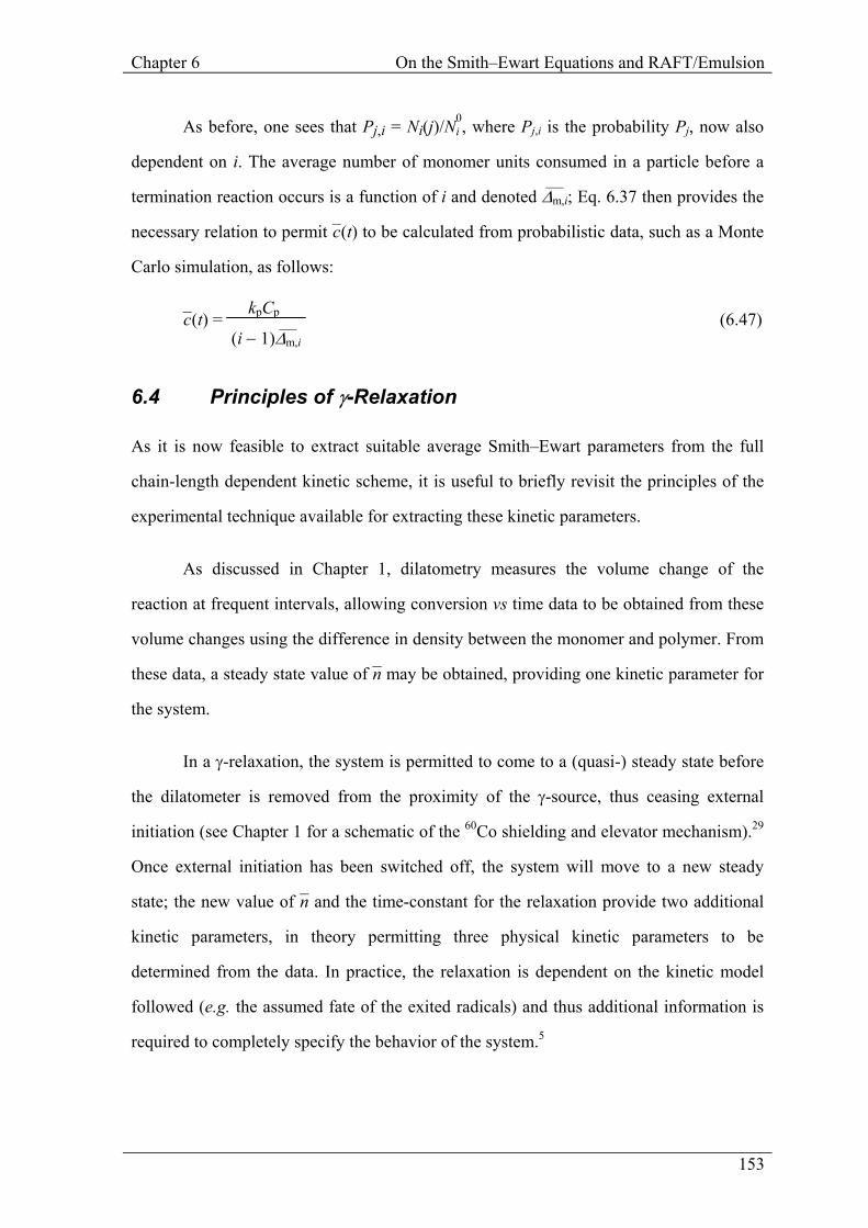
As before, one sees that Pj,i = Ni(j)/N0i , where Pj,i is the probability Pj, now also
dependent on i. The average number of monomer units consumed in a particle before a
termination reaction occurs is a function of i and denoted ∆m,i–– ; Eq. 6.37 then provides the
necessary relation to permit c–(t) to be calculated from probabilistic data, such as a Monte
Carlo simulation, as follows:
c–(t) = kpCp
(i − 1)∆m,i––
(6.47)
6.4 Principles of γ-Relaxation
As it is now feasible to extract suitable average Smith–Ewart parameters from the full
chain-length dependent kinetic scheme, it is useful to briefly revisit the principles of the
experimental technique available for extracting these kinetic parameters.
As discussed in Chapter 1, dilatometry measures the volume change of the
reaction at frequent intervals, allowing conversion vs time data to be obtained from these
volume changes using the difference in density between the monomer and polymer. From
these data, a steady state value of n– may be obtained, providing one kinetic parameter for
the system.
In a γ-relaxation, the system is permitted to come to a (quasi-) steady state before
the dilatometer is removed from the proximity of the γ-source, thus ceasing external
initiation (see Chapter 1 for a schematic of the 60Co shielding and elevator mechanism).29
Once external initiation has been switched off, the system will move to a new steady
state; the new value of n– and the time-constant for the relaxation provide two additional
kinetic parameters, in theory permitting three physical kinetic parameters to be
determined from the data. In practice, the relaxation is dependent on the kinetic model
followed (e.g. the assumed fate of the exited radicals) and thus additional information is
required to completely specify the behavior of the system.5
Chapter 6 On the Smith–Ewart Equations and RAFT/Emulsion
154
While UV radiation is sufficient to initiate bulk and solution polymerization
experiments, an emulsion polymerization has significant turbidity, preventing uniform
initiation throughout the latex with UV radiation. In contrast, γ-initiation is able to pass
through the latex with little attenuation, producing radicals homogeneously throughout
the reaction mixture.5
Previous well-documented uses of γ-initiation in RAFT-mediated polymerizations
include verifying that a polymerization follows RAFT-mediated kinetics rather than
“iniferter” kinetics30 and investigations of radical storage effects in the RAFT
mechanism.31 It has also been used for the creation of novel materials by initiating
grafting to substrates.32 Kinetic investigations using γ-relaxations have been performed on
emulsion polymerizations of monomers including styrene,29 methyl methacrylate,33 and
vinyl acetate.34
The numerical treatment of the dilatometry data with reference to possible
mechanisms for radical loss is described in Chapter 7, with additional information about
the mass-balance and model-independent kinetics used to treat the raw data contained in
the Appendices.
6.5 References
(1) Smith, W. V.; Ewart, R. H. J. Chem. Phys. 1948, 16, 592.
(2) Hawkett, B. S.; Napper, D. H.; Gilbert, R. G. J. Chem. Soc. Faraday Trans. 1 1977, 73, 690.
(3) Hawkett, B. S.; Napper, D. H.; Gilbert, R. G. J. Chem. Soc. Faraday Trans. 1 1980, 76, 1323.
(4) Ballard, M. J.; Gilbert, R. G.; Napper, D. H. J. Polym. Sci., Polym. Letters Edn. 1981, 19, 533.
(5) Gilbert, R. G. Emulsion Polymerization: A Mechanistic Approach; Academic: London, 1995.

Chapter 6 On the Smith–Ewart Equations and RAFT/Emulsion
155
(6) Lichti, G.; Gilbert, R. G.; Napper, D. H. J. Polym. Sci., Part A: Polym. Chem. 1980, 18, 1297.
(7) Adams, M. E.; Russell, G. T.; Casey, B. S.; Gilbert, R. G.; Napper, D. H.; Sangster, D. F. Macromolecules 1990, 23, 4624.
(8) Ugelstad, J.; Hansen, F. K. Rubber Chem. Technol. 1976, 49, 536.
(9) Casey, B. S.; Morrison, B. R.; Maxwell, I. A.; Gilbert, R. G.; Napper, D. H. J. Polym. Sci. A: Polym. Chem. 1994, 32, 605.
(10) Clay, P. A.; Gilbert, R. G. Macromolecules 1995, 28, 552.
(11) Stockmayer, W. H. J. Polym. Sci. 1957, 24, 314.
(12) O’Toole, J. T. J. Appl. Polym. Sci. 1965, 9, 1291.
(13) Morrison, B. R.; Casey, B. S.; Lacík, I.; Leslie, G. L.; Sangster, D. F.; Gilbert, R. G.; Napper, D. H. J. Polym. Sci. A: Polym. Chem. 1994, 32, 631.
(14) Napper, D. H.; Lichti, G.; Gilbert, R. G. In ACS Symp. Series - Emulsion Polymers and Emulsion Polymerization; Bassett, D. R., Hamielec, A. E., Eds.; American Chemical Society: Washington D.C., 1981; Vol. 165.
(15) de Kock, J. B. L.; Klumperman, B.; van Herk, A. M.; German, A. L. Macromolecules 1997, 30, 6743.
(16) de Kock, J. B. L.; van Herk, A. M.; German, A. L. J. Macromol. Sci., Polym. Rev. 2001, C41, 199.
(17) Russell, G. T. Aust. J. Chem. 2002, 55, 399.
(18) Clay, P. A.; Christie, D. I.; Gilbert, R. G. In ACS Symp. Series - Advances in Free-Radical Polymerization; Matyjaszewski, K., Ed.; American Chemical Society: Washington D.C., 1998; Vol. 685.
(19) Clay, P. A.; Gilbert, R. G.; Russell, G. T. Macromolecules 1997, 30, 1935.
(20) Russell, G. T.; Napper, D. H.; Gilbert, R. G. Macromolecules 1988, 21, 2133.
(21) Griffiths, M. C.; Strauch, J.; Monteiro, M. J.; Gilbert, R. G. Macromolecules 1998, 31, 7835.
(22) Clay, P. A.; Gilbert, R. G. Macromolecules 1995, 28, 552.
Chapter 6 On the Smith–Ewart Equations and RAFT/Emulsion
156
(23) Scheren, P. A. G. M.; Russell, G. T.; Sangster, D. F.; Gilbert, R. G.; German, A. L. Macromolecules 1995, 28, 3637.
(24) Maxwell, I. A.; Morrison, B. R.; Napper, D. H.; Gilbert, R. G. Macromolecules 1991, 24, 1629.
(25) de Gennes, P. G. J. Chem. Phys. 1971, 55, 572.
(26) Casey, B. S.; Mills, M. F.; Sangster, D. F.; Gilbert, R. G.; Napper, D. H. Macromolecules 1992, 25, 7063.
(27) Maeder, S.; Gilbert, R. G. Macromolecules 1998, 31, 4410.
(28) Prescott, S. W. Macromolecules 2003, ASAP, DOI: 10.1021/ma034845h.
(29) Lansdowne, S. W.; Gilbert, R. G.; Napper, D. H.; Sangster, D. F. J. Chem. Soc. Faraday Trans. 1 1980, 76, 1344.
(30) Quinn, J. F.; Barner, L.; Davis, T. P.; Thang, S. H.; Rizzardo, E. Macromol. Rapid Commun. 2002, 23, 717.
(31) Barner-Kowollik, C.; Vana, P.; Quinn, J. F.; Davis, T. P. J. Polym. Sci., Part A: Polym. Chem. 2002, 40, 1058.
(32) Barner, L.; Zwaneveld, N.; Perera, S.; Pham, Y.; Davis, T. P. J. Polym. Sci., Part A: Polym. Chem. 2002, 40, 4180.
(33) Ballard, M. J.; Napper, D. H.; Gilbert, R. G.; Sangster, D. F. J. Polym. Sci. Polym. Chem. Edn. 1986, 24, 1027.
(34) De Bruyn, H.; Gilbert, R. G.; Ballard, M. J. Macromolecules 1996, 29, 8666.


![[Scherma] - Ewart Oakeshott - Sword in the Age of Chivalry](https://img.pdfslide.us/doc/110x75/55cf9bf4550346d033a800d4/scherma-ewart-oakeshott-sword-in-the-age-of-chivalry.jpg)