Embed Size (px)
Citation preview
Advances in Mathematics 256 (2014) 449–478
Contents lists available at ScienceDirect
Advances in Mathematics
www.elsevier.com/locate/aim
On the reconstruction problem in mirror symmetry
Junwu TuMathematics Department, University of Oregon, Eugene, OR 97403, USA
a r t i c l e i n f o a b s t r a c t
Article history:Received 2 September 2012Accepted 11 February 2014Available online 4 March 2014Communicated by Bernd Siebert
Keywords:Maurer–CartanA-infinityFloer
Let π : M → B be a Lagrangian torus fibration withsingularities such that the fibers are of Maslov index zero,and unobstructed. The paper constructs a rigid analytic spaceM∨
0 over the Novikov field which is a deformation of thesemi-flat complex structure of the dual torus fibration overthe smooth locus B0 ⊂ B of π. Transition functions of M∨
0are obtained via A∞ homomorphisms which capture the wall-crossing phenomenon of moduli spaces of holomorphic disks.
© 2014 Elsevier Inc. All rights reserved.
1. Introduction
1.1. Background
Let (M,ω) be a symplectic manifold endowed with a (special) Lagrangian torus fi-bration π : M → B possibly with singularities. Given such a fibration (plus additionalpolarization data), the reconstruction problem in mirror symmetry concerns about con-structing a complex manifold M∨ which conjecturally should be a mirror partner for M .As such this problem lies at the heart towards a mathematical understanding of themysterious mirror duality.
The reconstruction problem was first discussed by Kontsevich and Soibelman in [13,Section 7.1, Remark 19]. Later on in a series of remarkable papers [9–11] Mark Gross and
E-mail address: [email protected].
http://dx.doi.org/10.1016/j.aim.2014.02.0050001-8708/© 2014 Elsevier Inc. All rights reserved.
450 J. Tu / Advances in Mathematics 256 (2014) 449–478
Bernd Siebert initiated, and studied in depth this problem from a more combinatorialpoint of view (a global version of toric geometry). There are also nice concrete exampleswhere this reconstruction process is explicitly realized, see for instance [1] by Auroux,and [3] by Chan–Lau–Leung.
At the same time, Fukaya, Oh, Ono, and Ohta are developing Lagrangian Floer theoryand its obstruction theory [7]. After their work it has become evident that the homotopytheory of A∞ algebras is the right language for Lagrangian Floer theory. For example,associated with a (spin) Lagrangian submanifold L in a symplectic manifold M one candefine an A∞ algebra structure on the de Rham complex of L with coefficients in certainNovikov ring. This construction involves various choices that makes this A∞ structurenot an invariant of symplectic geometry of the pair (M,L). However the upshot is thatthe homotopy type of this structure is a symplectic invariant!
Later on in [4], inspired by Lagrangian Floer theory, Fukaya briefly outlined a moreconceptual approach to understand the reconstruction problem via gluing of Maurer–Cartan moduli spaces associated A∞ algebras. It is expected that once this constructionis properly understood, homological mirror symmetry conjecture will follow from it withless efforts (see [14] for the local situation).
1.2. The current work
In this paper we carry out Fukaya’s approach to deal with the reconstruction problemover the smooth locus B0 ⊂ B of a Lagrangian torus fibration π : M → B under certainassumptions. Our main result is the following theorem. We refer to Corollary 4.10 inSection 4 for a more precise formulation of it.
Theorem 1.1. Assume that Lagrangian torus fibers over B0 are unobstructed, and areof Maslov index zero in (M,ω). Then there is a natural construction of a rigid ana-lytic space M∨
0 over the Novikov field Λ fibered over B0, which gives a deformation ofKontsevich–Soibelman’s construction [13, Section 7, Definition 22].
Remark. The idea to use non-Archimedean geometry to deal with possible convergenceissues in Floer theory is due to Kontsevich and Soibelman [13]. Namely the mirrormanifold M∨ to be constructed should not be a complex manifold over C, but rather arigid analytic space over a valuation ring.
Remark. The explicit gluing formulas (4.12) in the construction of M∨0 involves certain
instanton corrections from symplectic geometry. If the instanton corrections were notpresented, then these formulas reduce to the one used in [13]. We also note that for theconstruction of M∨
0 we do not need a polarization data on M . Such a polarization seemsto be related to constructing a compactification of the space M∨
0 . At present, we do notknow how to do this.
J. Tu / Advances in Mathematics 256 (2014) 449–478 451
Remark. The Maslov index zero condition is automatic for special Lagrangian torusfibrations in a Calabi–Yau manifold. However the unobstructedness assumption is notknown in that case, even though expected. On the other hand, in view of [14], the unob-structedness assumption is necessary for the purpose of homological mirror symmetry.Indeed without this assumption the Maurer–Cartan moduli spaces involved carry too lessinformation in order to have an equivalence predicted by homological mirror symmetry.
2. Algebraic framework
In this section we recall certain homotopy theory of gapped and filtered A∞ algebrasdeveloped by Fukaya in [4]. Another reference is Fukaya’s joint work with Oh, Ohta andOno [7]. The construction of canonical models in the gapped and filtered context wasfirst discussed in [5], see also [7] and [4].
2.1. Monoids
Since our primary geometric applications concern only Lagrangians with vanishingMaslov index, we shall work with a monoid G ⊂ R
�0 which keeps track of the energy ofpseudo-holomorphic curves.1 In view of Gromov’s compactness theorem we require that
∣∣G ∩ [0, E]∣∣ < ∞, ∀E ∈ R
�0.
Given such a monoid G we can form a ring ΛC
G consisting of formal sums of the form∑∞i=0 aiT
βi such that ai ∈ C, βi ∈ G. The finiteness condition above implies that
∣∣{i | ai �= 0, βi � E}∣∣ < ∞, ∀E ∈ R
�0.
We define a valuation on ΛC
G by
val( ∞∑
i=0aiT
βi
):= inf
{i|ai �=0}βi.
This valuation map induces a filtration on ΛC
G by setting
FE(ΛC
G
):=
{a ∈ ΛC
G
∣∣ val(a) � E}
for a fixed energy E ∈ R�0. This filtration defines a topology on the ring ΛC
G, making it atopological ring (i.e. its product is continuous with respect to the topology). Furthermorethe ring ΛC
G is complete with respect to this topology.
1 In [4] and [7] the authors used monoids in R�0 × 2Z in which the component 2Z keeps track of the
Maslov index.
452 J. Tu / Advances in Mathematics 256 (2014) 449–478
2.2. Gapped filtered A∞ algebras
Let (V ,D, ◦) be a differential graded algebra over C, and denote by BV its cobardifferential graded coalgebra. Explicitly BV is the free graded coalgebra T(V [1]) endowedwith a degree one coderivation Q0 determined by two degree one linear maps
D : V [1] → V [1]
◦ : V [1] ⊗ V [1] → V [1].
Consider a monoid G as explained above, and form the tensor product
V := V ⊗̂ ΛC
G.
Here ⊗̂ stands for first taking ordinary tensor product, and then taking topologicalcompletion with respect to the topology induced from the filtration mentioned above.Explicitly elements of V are of the form
∑∞i=0 viT
βi where vi ∈ V and βi ∈ G. Theseseries are required to satisfy the same finiteness condition as in the definition of ΛC
G.The linear space V also has a valuation map defined in the same way as that of ΛC
G.With the induced topology the ΛC
G-module structure on V is continuous.For later usage we shall call elements with strictly positive valuations positive. For
example, positive elements of V are formal series such that the coefficient of T 0 is zero.We extend the differential D and the product ◦ on V to the whole space V by
ΛC
G-linearity to obtain a differential graded algebra structure on V over ΛC
G. Denoteby BV its cobar construction, and again by Q0 its cobar differential.
Definition 2.1. A G-gapped filtered A∞ algebra structure on V is a degree one, positiveΛC
G-linear coderivation δ on the coalgebra BV := T(V [1]) such that
(Q0 + δ)2 = 0
Remark. Equivalently the element δ may be considered a positive Maurer–Cartan elementof the differential graded Lie algebra Coder(BV ) where we consider the standard Liestructure on Coder(BV ), and its differential is given by [Q0,−]. Indeed sine the differentialQ0 on Coder(BV ) squares to zero, the equation (Q0 + δ)2 = 0 is equivalent to [Q0, δ] +12 [δ, δ] = 0 which is precisely the Maurer–Cartan equation of Coder(BV ).
2.3. Explicit formula for A∞ algebras
Let us unwind the definition of a G-gapped filtered A∞ structure in terms of multi-linear maps on V . For this note that there is a bijection between the two sets
Coder(BV ) ↔ Hom(BV, V ) =∞∏
Hom(V [1]k, V [1]
)
k=0
J. Tu / Advances in Mathematics 256 (2014) 449–478 453
which sends an element ϕ ∈ Coder(BV ) to π ◦ ϕ where π : BV → V [1] is the canonicalprojection map. The backward map is given by extending a given multi-linear map inHom(V [1]k, V [1]) by the co-Leibniz rule to a coderivation on BV . Denote by mk the com-ponent in Hom(V [1]k, V [1]) corresponding to the coderivation (Q0 + δ) in Definition 2.1.The continuous ΛC
G-linear map mk : V [1]k → V [1] can be written as
mk =∑β∈G
mk,βTβ
for C-linear maps mk,β : V [1]k → V [1] of degree one. The positivity of δ implies that
mk,0 =
⎧⎨⎩
D k = 1◦ k = 20 otherwise.
(2.1)
Written in terms of mk,β the equation (Q0 + δ)2 gets translated into the equations∑
i+j+k=N,i�0,j�0,k�0
∑β1+β2=β
mi+k+1,β1
(idi ⊗mj,β2 ⊗ idk
)= 0 (2.2)
for all N � 0, β ∈ G. Here Koszul sign convention is assumed when forming tensorproducts of linear maps.
2.4. Pseudo-isotopies of A∞ algebras
Let Ω∗Δ1 be the set of C∞ differential forms on the 1-simplex Δ1 = [0, 1] that are
constant in a neighborhood of 0 and 1. The boundary condition is due to a technicalreason: being able to perform gluing of pseudo-isotopies in the smooth category.
Definition 2.2. A pseudo-isotopy between two G-gapped filtered A∞ algebra structuresδ0 and δ1 on V is given by a positive Maurer–Cartan element γ ∈ MC(Coder(BV )⊗̂Ω∗
Δ1).The element γ is required to satisfy the boundary conditions
i∗0γ = δ0, and i∗1γ = δ1.
Here the maps i∗j denote pull-backs of differential forms via the inclusions ij : j → [0, 1]for j = 0, or 1.
Lemma 2.3. Pseudo-isotopy defines an equivalence relation on the set of all G-gappedfiltered A∞ structures on V .
Proof. Let δ be an A∞ algebra structure, then γ = δ viewed as a “constant” ele-ment of Coder(BV ) ⊗ Ω∗
Δ1 is a pseudo-isotopy between δ and itself. Reversing a givenpseudo-isotopy γt �→ γ1−t proves reflexive property. For the transitivity let γ1 be a
454 J. Tu / Advances in Mathematics 256 (2014) 449–478
pseudo-isotopy between δ0 and δ1. Let γ2 be another pseudo-isotopy between δ1 and δ2.There are the following two maps between intervals
λ1 : [0, 1/2] → [0, 1], t �→ 2t;
λ2 : [1/2] → [0, 1], t �→ 2t− 1.
Then λ∗1γ1 and λ∗
2γ2 are differential forms on [0, 1/2] and [1/2, 1] with values in the Liealgebra Coder(BV ). Moreover they are both δ1 in a neighborhood of 1/2. Hence we canglue them to form a C∞ form on [0, 1] with values in Coder(BV ). We denote the resultof this gluing by γ1�γ2 to mimic the “concatenation of paths” in topology. Then γ1�γ2is a pseudo-isotopy between δ0 and δ2. The lemma is proved. �2.5. Explicit formula for pseudo-isotopies
Let δ0, δ1 be two A∞ structures on V , and denote by m0k, m1
k the correspondingmulti-linear maps on V [1]. A pseudo-isotopy γ between δ0 and δ1 is a Maurer–Cartanelement of the form
γ = δt + ht dt
for some positive elements δt, ht ∈ Coder(BV ) ⊗̂C∞([0, 1]) such that δt is of degree one,ht is of degree zero, satisfying the initial condition
δt|t=0 = δ0, and δt|t=1 = δ1.
Moreover the Maurer–Cartan equation for γ implies that⎧⎨⎩
[Q0 + δt, Q0 + δt
]= 0,
dδt
dt=
[Q0 + δt, ht
].
Let mtk,β and ht
k,β be the associated multi-linear maps on V [1] corresponding to thecoderivations Q0 + δt and ht. The positivity of γ = δt + ht dt implies that mt
k,0 is asin Eq. (2.1) for all t ∈ [0, 1], and ht
k,0 ≡ 0. In terms of these component maps, thefirst equation above says that mt
k =∑
β mtk,β form a family of G-gapped filtered A∞
structure on V . The second equation can be expanded to get
dmtN,β
dt= −
∑i+j+k=N
∑β1+β2=β
mti+k+1,β1
(idi ⊗ ht
j,β2⊗ idk
)
+∑
i+j+k=N
∑β1+β2=β
hti+k+1,β1
(idi ⊗mt
j,β2⊗ idk
)(2.3)
where the equation holds for all N � 0, and β ∈ G.
J. Tu / Advances in Mathematics 256 (2014) 449–478 455
2.6. From pseudo-isotopies to A∞ homomorphisms
Recall a filtered A∞ homomorphism from (A, δA) to (B, δB) is a continuous map ofdifferential graded coalgebras F : BA → BB. If mA
k,β and mBk,β are the corresponding
structure constants for δA and δB , the map F can be realized as multi-linear mapsFk,β : (A[1])k → B[1] of degree zero satisfying
∑0�j,i1+···+ij=N
∑β0+βi1+···+βij
=β
mBj,β0
(Fi1,βi1⊗ · · · ⊗ Fij ,βij
)
=∑
i+j+k=N
∑β1+β2
Fi+k+1,β1
(idi ⊗mA
j,β2⊗ idk
)(2.4)
where the equation holds for all N � 0, and β ∈ G.Given a pseudo-isotopy γ between (V, δ0) and (V, δ1) we can construct an A∞ homo-
morphism from (V, δ0) to (V, δ1), which we now explain. We need a few ingredients forthis construction.
2.7. Stable trees with decorations
Let k � 0 be a nonnegative integer. Consider a rooted ribbon tree T with k leaves.Here the word “ribbon” means that, for every vertex of the tree, a cyclic ordering isassigned to the set of half edges incident to that vertex. The root of a tree T will bedenoted by rT , the set of edges by E(T ), and the set of vertices by V (T ). We remark thatthe set V (T ) is the disjoint union of V int(T ) consisting of interior vertices and V ext(T )consisting of k + 1 exterior vertices (corresponding to the root and the k leaves). Theexterior vertices are necessarily of valency 1, for the interior vertices we allow them tohave arbitrary positive valency. A G-decoration on T is a map λ : V int(T ) → G. We calla G-decorated ribbon tree stable if every interior vertex decorated by 0 ∈ G has at leastvalency 3. We denote by O(k, β) be the set of stable G-decorated rooted ribbon treeswith k leaves such that
∑v∈V int(T )
λ(v) = β.
Lemma 2.4. The set O(k, β) is a finite set for all k � 0, and β ∈ G.
Proof. It suffices to show that the number of the set V int(T ) is finite. By the finitenessassumption on the monoid G this is equivalent to show that the set of interior ver-tices decorated by 0 ∈ G is finite. For this we observe that since T is a tree which iscontractible, hence its Euler characteristic is
(k + 1) +∣∣V int(T )
∣∣− ∣∣E(T )∣∣ = 1.
456 J. Tu / Advances in Mathematics 256 (2014) 449–478
Denote by x the number of vertices decorated by zero, and by y the rest interior vertices.So we have x + y = |V int(T )|. By the stableness assumption there are at least 3x halfedges incident to these vertices. Thus |E(T )| � 3x/2, together with the above qualities,implies that x � 2(k + y). Since the right hand side is bounded, x is also bounded. Thelemma is proved. �
Let (T, λ) ∈ O(k, β) be a stable G-decorated tree. We define a partial ordering onthe set V int(T ) as follows. We say v1 � v2 if v2 is contained in the shortest path fromv1 to the root rT . Here we measure a path by its number of edges in T . Let t ∈ [0, 1],a time ordering on T bounded by t is a non-decreasing map τ : V int(T ) → [0, t]. Sincethis partial ordering only depends on the tree T , and not on the decoration λ, we denoteby M t(T ) the set of all time orderings on T . We endow it with the subset topologyof [0, t]|V int(T )|. As such it is compact. The Euclidean measure on [0, t]|V int(T )| induces ameasure on M t(T ) which we denote by dτ .
For each triple (T, λ, τ) we will define a multi-linear map ρ(T, λ, τ) : V [1]k → V [1] ofdegree zero. On each internal vertex v ∈ V int(T ) we put the linear map h
τ(v)val(v)−1,λ(v) where
val(v) is the valency of the vertex v. Then the map ρ(T, λ, τ) is simply the “operadic”composition of these linear maps according to the tree T .
Finally we can define the structure maps F tk,β : V [1]k → V [1] of an A∞ homomorphism
by
F tk,β :=
∑(T,λ)∈O(k,β)
ρt(T, λ) where ρt(T, λ) :=∫
M t(T )
ρ(T, λ, τ) dτ. (2.5)
By the previous lemma this is only a finite sum, hence is well-defined. The main propertyfor these complicatedly defined maps is the following derivative formula.
Lemma 2.5. For each (T, λ) ∈ O(k, β) we have the following formula
dρt(T, λ)dt
= htl,λ(v0)
[ρt(T (1), λ(1))⊗ · · · ⊗ ρt
(T (l), λ(l))].
Here the vertex v0 is the unique vertex connected the root of T , and the trees T (1), . . . , T (l)
are obtained so that μl ◦ (T (1) ⊗ · · · ⊗ T (l)) = T where μl denote the star graph with l
inputs. Namely if we glue the roots of T (i)’s into the inputs of μl, we obtain the tree T .Decorations λ(1), . . . , λ(l) are induced from that of λ.
Proof. The integral∫
M t(T ) ρ(T, λ, τ) dτ , by its definition, may be rewritten as
t∫0
hτ(v0)l,λ(v0) ◦
[ρτ(v0)
(T (1), λ(1))⊗ · · · ⊗ ρτ(v0)
(T (l), λ(l))]dτ(v0).
The lemma then follows from fundamental theorem of calculus. �
J. Tu / Advances in Mathematics 256 (2014) 449–478 457
Lemma 2.6. The maps F tk defined by formula (2.5) form an A∞ homomorphism F :
(V,m0) → (V,mt).
Proof. By formula (2.4) we need to compare the following two terms for all n � 0, andβ ∈ G:
Itn,β :=∑
i+k+j=n
∑β1+β2=β
F ti+j+1,β1
(idi ⊗m0
k,β2⊗ idj
);
II tn,β :=
∑i1+···+ik=n
∑β0+βi1+···+βik
=β
mtk
(F ti1,βi1
⊗ · · · ⊗ F tik,βik
).
Denote by Δtn,β := Itn,β − II t
n,β their difference. Computing dΔtn,β
dt using formula (2.3)and Lemma 2.5 yields
dΔtn,β
dt=
∑i1+···+ij+l+k=n
∑β0+β1+βi1+···+βij+l
=β
htj+l+1,β0
(F ti1,βi1
⊗ · · · ⊗ F tij ,βij
⊗Δtk,β1
⊗ F tij+1,βij+1
⊗ · · · ⊗ F tij+l,βij+l
).
Moreover we have the initial conditions Δ0n,β = 0, and Δt
n,0 = 0 for all n � 0, β ∈ G.In the case n = 0, we can proceed the proof by doing induction on β. Indeed Δt
n,0serves as the initial step of the induction. For higher β observe that the right hand sidereduces to an ordinary differential equation by induction. Hence by uniqueness of solutionof ordinary differential equations Δt
0,β ≡ 0. In general we can proceed by induction alsoon the variable n, namely we assume Δt
k,β ≡ 0 for all k � n and β < E. Here E is takenso that E ∈ G and (β,E) contains no other element in G. In this case we can showthat Δn,E is zero which again follows from uniqueness of solution of ordinary differentialequations. Thus the lemma is proved. �2.8. Nerve of Coder(BV )
Consider smooth differential forms Ω∗Δn on the standard n-simplex Δn := {(t0, . . . , tn)
∈ Rn+1 | ti � 0,
∑ti = 1} that are constant in a neighborhood of the vertices of Δn.
Let V be as before, and denote by g the graded Lie algebra Coder(BV ) consisting ofcontinuous coderivations. We have considered the Maurer–Cartan elements of g⊗Ω∗
Δ0 =g which are A∞ structures on V , and that of g⊗Ω∗
Δ1 which are pseudo-isotopies betweenA∞ structures.
The spaces MC(g) and MC(g ⊗ Ω∗Δ1) are only “pieces of an iceberg”. Indeed the
collection of differential graded Lie algebras {g⊗Ω∗Δn}∞n=0 form a simplicial differential
graded Lie algebra g∗. Applying the Maurer–Cartan functor to it yields a simplicialset Σ∗g := MC(g∗), which was introduced by Hinich [12] and further investigated byGetzler [8].
458 J. Tu / Advances in Mathematics 256 (2014) 449–478
Intuitively elements of Σ∗g = MC(g⊗Ω∗Δn) for n � 2 are pseudo-isotopies of pseudo-
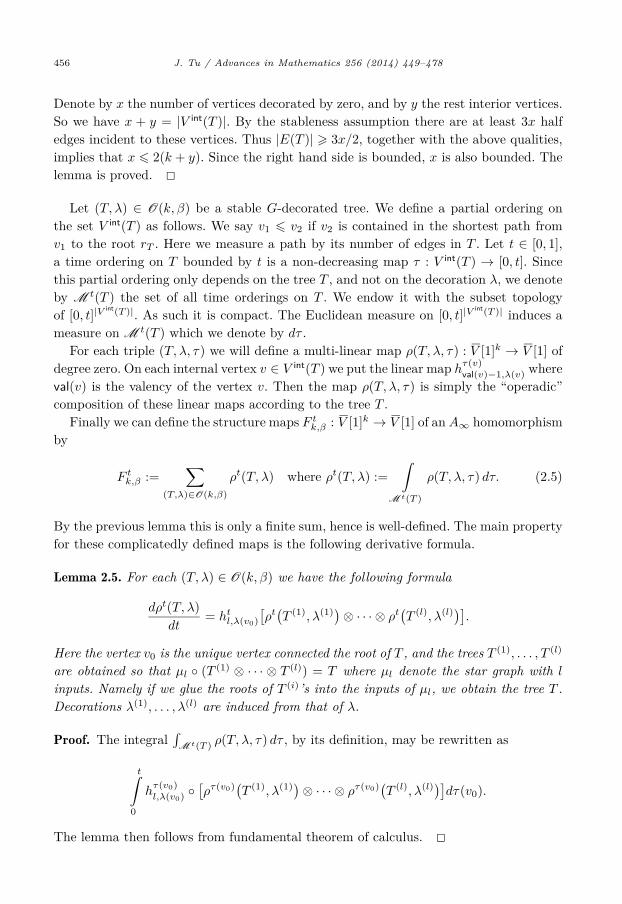
isotopies. We may think of elements of Σ0g as points, and elements of Σ1g as pathsbetween these points.
γ(0) := i∗0γ = δ0 • γ−→ • γ(1) := i∗1γ = δ1
Similarly elements of Σ2g are homotopies of paths, and elements of Σ3g are homotopiesof homotopies of paths, and so on. In the following we shall call an element of Σng ann-pseudo-isotopy. For the purposes of this paper we only need to consider the cases forn � 2.
2.9. From 2-pseudo-isotopies to homotopies of A∞ morphisms
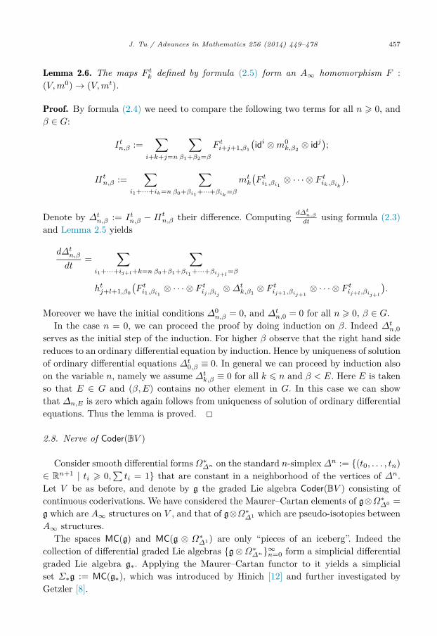
Let α ∈ Σ2g be a 2-pseudo-isotopy, and let ∂0(α), ∂1(α), ∂2(α) be its boundarypseudo-isotopies.
δ0 δ2
δ1
α
∂2(α)
∂1(α)
∂0(α)
Theorem 2.7. The two A∞ morphisms F [∂1(α)] and F [∂0(α)] ◦ F [∂2(α)] obtained fromboundary 1-pseudo-isotopies of α are homotopic homomorphisms (see [7, Chapter 4] forthe notion of homotopy used here).
Proof. Let u : [0, 1]s × [0, 1]t → Δ2 be an orientation preserving smooth map with thefollowing boundary conditions:
u(0 × [0, 1]
)= 0;
u(1 × [0, 1]
)= 2;
u([0, 1] × 0
)= ∂1;
u([0, 1] × 1
)= ∂2 ∪ ∂0.
Here on the right hand side of these equations the notations are illustrated in the figureabove. Then the t-direction defines a homotopy between F [∂1(α)] and F [∂0(α)]◦F [∂2(α)].The lemma is proved. �
J. Tu / Advances in Mathematics 256 (2014) 449–478 459
2.10. Canonical models
In the rest of this section we recall a few formulas for doing homological perturba-tion for G-gapped filtered A∞ algebras and their pseudo-isotopies. These formulas areimportant because we need to use their cyclic symmetry and exponential dependence inthe next section.
Recall we have a differential graded algebra (V ,D, ◦) on the zero energy part of aG-gapped filtered A∞ algebra V = V ⊗̂ ΛC
G. Let us denote by H the cohomology ofthe complex (V,D). Consider linear maps i : H → V , p : V → H of degree zero, andh : V → V of degree −1 satisfying conditions
Di = 0, pD = 0, pi = id, id − ip = Dh + hD.
Such a triple (i, p, h) is called a deformation retraction. Given a G-gapped filtered A∞algebra V and a deformation retraction (i, p, h) on V , we can construct a G-gappedfiltered A∞ algebra structure on H := H ⊗C ΛC
G. This is known as the canonical modelfor V .
We describe this G-gapped filtered A∞ algebra on H by providing explicit formulasfor mcan
k,β . For this let (T, λ) ∈ O(k, β) be a G-decorated ribbon tree with k leaves. Weassociate to each interior vertex v ∈ V int(T ) the operator mval(v)−1,λ(v), to each interioredge (edges that are not connected to a leave or the root) the homotopy operator h,to each leaf the embedding i, and finally to the unique edge incident to the root theprojection map p. Define η(T, λ) as the operadic composition of these multi-linear maps.Then the structure maps mcan
k,β on H is defined as
mcank,β :=
∑(T,λ)∈O(k,β)
η(T, λ). (2.6)
Let γ = δ + h dt ∈ Σ1g be a 1-pseudo-isotopy on V , and let mtk,β , ht
k,β be its associatedstructure maps. We shall define γcan which is a 1-pseudo-isotopy on H. The formula formt,can
k,β is given by Eq. (2.6) above allowing the parameter t to enter.The formula for ht,can
k,β is defined as follows. Consider O+(k, β) the set of triples (T, λ, v)where (T, λ) is a G-decorated ribbon trees with k leaves in O(k, β), and v ∈ V int(T ) achosen interior vertex of T . Then we associate operators to this triple (T, λ, v) in thesame way as in the construction of mcan
k,β except at the chosen vertex we put the operatorht
val(v)−1,λ(v). Define μ(T, λ, v) to be the operadic composition, and the formula for ht,cank,β
is defined by
ht,cank,β :=
∑(T,λ,v)∈O+(k,β)
μ(T, λ, v). (2.7)
460 J. Tu / Advances in Mathematics 256 (2014) 449–478
2.11. Maurer–Cartan moduli spaces
An important homotopy invariant associated with a G-gapped filtered A∞ algebrais its Maurer–Cartan moduli space. As before we use mk,β , and mk :=
∑β mk,β for
structure maps of a G-gapped filtered A∞ structure δ on V . Furthermore we denote byΛ+G consisting of elements in ΛC
G of positive valuation, and denote by V + := V ⊗ Λ+G.
Let b ∈ V + be a positive element of degree one. The Maurer–Cartan equation isdefined as
m0 + m1(b) + m2(b2)
+ · · · + mk
(bk)
+ · · · = 0.
Note that the fact that b has positive valuation ensures the convergence of this equation.Solutions of this equation are called Maurer–Cartan elements of V . Two Maurer–Cartanelements b0 and b1 are called gauge equivalent if there exists a Maurer–Cartan elementθ ∈ V ⊗Ω∗
Δ1 such that θ is positive, and satisfies
i∗0θ = b0, and i∗1θ = b1.
More explicitly the element θ is of the form θ = b(t) + c(t) dt for a one parameter degreeone positive element b(t), and one parameter degree zero element c(t). They are subjectto the following equations⎧⎪⎪⎨
⎪⎪⎩m0 + m1
(b(t)
)+ · · · + mk
(b(t)k
)+ · · · = 0,
db(t)dt
+∞∑k=0
∑i+j=k
mk+1(b(t)i, c(t), b(t)j
)= 0. (2.8)
Lemma 2.8. Gauge equivalence is an equivalence relation.
The lemma is proved in [7]. The Maurer–Cartan moduli space MC+(V, δ)2 of an A∞algebra (V, δ) is then defined as the set of equivalence classes of Maurer–Cartan elementsmodulo gauge equivalence. The fundamental property of the assignment sending
A∞ algebra (V, δ) �→ MC+(V, δ)
is that it factor through the homotopy category of A∞ structures on V . In particular ho-motopy equivalent A∞ structures have isomorphic Maurer–Cartan moduli spaces. Moreexplicitly if Φ : A → B is a map of G-gapped filtered A∞ homomorphism, then the map
b �→ Φ0(1) + Φ1(b) + Φ2(b2)
+ · · · + Φk
(bk)
+ · · · (2.9)
respects gauge equivalence, which descends to a map Φ∗ : MC+(A) → MC+(B). In casewhen Φ is a homotopy equivalence this map is an isomorphism. In particular if γ is
2 Here we added a plus sign to indicate that we only consider elements of positive valuation.
J. Tu / Advances in Mathematics 256 (2014) 449–478 461
a 1-pseudo-isotopy between two A∞ algebra structures δ0 and δ1 on V , then the A∞homomorphism F (γ) : (V, δ0) → (V, δ1) defined earlier induces an isomorphism on theassociated Maurer–Cartan moduli spaces.
3. Geometric realizations
3.1. A∞ algebras associated with Lagrangian submanifolds
Let L be a relatively spin compact Lagrangian submanifold in a symplectic manifold(M,ω). In [7] and [4] a curved A∞ algebra structure was constructed on Ω∗(L,Λ0),the de Rham complex of L with coefficients in certain Novikov ring Λ0 over C.3 Herecoefficient ring Λ0 is defined by
Λ0 :={ ∞∑
i=1aiT
λi
∣∣∣ ai ∈ C, λi ∈ R�0, lim
i→∞λi = ∞
}
where T is a formal parameter of degree zero. To make connections with the ring ΛC
G
used in the previous section, we observe that there is an inclusion of monoids
G ↪→ R�0,
which induces an inclusion of rings ΛC
G ↪→ Λ0. The A∞ algebra associated with L can beconstructed over ΛC
G for some monoid G depending on L. By extension of scalars we getan A∞ algebra over Λ0. We shall refer to this A∞ algebra as the Fukaya (A∞) algebraof L.
Note that the map val : Λ0 → R defined by val(∑∞
i=1 aiTλi) := infai �=0λi endows Λ0
with a valuation ring structure. Denote by Λ+0 the subset of Λ0 consisting of elements
with strictly positive valuation. This is the unique maximal ideal of Λ0. In [7] there wasan additional parameter e to encode Maslov index to have a Z-graded A∞ structure. Ifwe do not use this parameter, we need to work with Z/2Z-graded A∞ algebras.
We briefly recall the construction of the Fukaya A∞ algebra structure on Ω∗(L,Λ0).Let β ∈ π2(M,L) be a class in the relative homotopy group, and choose an almostcomplex structure J compatible with (or simply tamed) ω. Form Mk+1,β(M,L; J), themoduli space of stable (k+1)-marked J-holomorphic disks in M with boundary lying inL0 of homotopy class β with suitable regularity condition in interior and on the boundary.The moduli space Mk+1,β(M,L; J) is of virtual dimension d + k + μ(β) − 2 (here μ(β)is the Maslov index of β).
3 Strictly speaking this version of Floer theory was developed by K. Fukaya in [4] heavily based on thework of himself, Y.-G. Oh, H. Ohta and K. Ono [7].
462 J. Tu / Advances in Mathematics 256 (2014) 449–478
There are (k + 1) evaluation maps evi : Mk+1,β(M,L; J) → L for i = 0, . . . , k whichcan be used to define a map mk,β : (Ω∗(L,C)⊗k) → Ω∗(L,C) of form degree 2−μ(β)−k
by formula
mk,β(α1, . . . , αk) := (ev0)!(ev∗1α1 ∧ · · · ∧ ev∗kαk
).
To get an A∞ algebra structure we need to combine mk,β for different β’s. For thispurpose we define a submonoid G(L) of R�0 × 2Z as the minimal one generated by theset
{(∫β
ω, μ(β))
∈ R�0 × 2Z
∣∣∣ β ∈ π2(M,L),M0,β(M,L; J) �= ∅}.
Then we can define the structure maps mk : (Ω(L,Λ0))⊗k → Ω(L,Λ0) by
mk(α1, . . . , αk) :=∑
β∈G(L)
mk,β(α1, . . . , αk)T∫βω.
Note that we need to use the Novikov coefficients here since the above sum might notconverge for a fixed value of T . The boundary stratas of Mk+1,β(M,L; J) are certainfiber products of the diagram
Mi+1,β1(M,L; J) ×L Mj+1,β2(M,L; J) −−−−→ Mj+1,β2(M,L; J)⏐⏐� ⏐⏐�evl
Mi+1,β1(M,L; J)ev0−−−−→ L.
Here 1 � l � j, i + j = k + 1, and β1 + β2 = β. Indeed using this description of theboundary stratas the A∞ axiom for structure maps mk is an immediate consequence ofStokes formula.
We should emphasize that a mathematically rigorous realization of the above ideas in-volves lots of delicate constructions. Indeed the moduli spaces involved Mk+1,β(M,L; J)are not smooth manifolds, but Kuranishi orbifolds with corners, which causes trouble todefine an integration theory. Even if this regularity problem is taken of there are stilltransversality issues to define maps mk,β to have the expected dimension. Moreover itis not enough to take care of each individual moduli space since the A∞ relations formk follows from analyzing the boundary stratas in Mk+1,β(M,L; J). Thus one needs toprove transversality of evaluation maps that are compatible for all k and β. Furthermoreone also needs to deal with not only disk bubbles, but also sphere bubbles and regularityand transversality issues therein. We refer to the original constructions of [7] and [4] forsolutions of these problems.
J. Tu / Advances in Mathematics 256 (2014) 449–478 463
3.2. Geometric realization of pseudo-isotopies
We shall apply the algebraic constructions in the previous section in the case V =Ω∗(L,C) is the de Rham differential graded algebra. In the construction of the Fukayaalgebra of L we need to make a choice of an ω-tamed almost complex structure on M .One of the main results in [4] is that this A∞ algebra is uniquely determined up topseudo-isotopies.
Indeed if J0 and J1 are two ω-tamed almost complex structures we may choose a pathJt (t ∈ [0, 1]) of almost complex structures connecting them. This is always possiblesince the space of ω-tamed almost complex structures is contractible, and hence pathconnected. Consider the parametrized moduli spaces
Mk+1,β(M,L; J ) :=∐
t∈[0,1]
t× Mk+1,β(M,L; Jt).
Again we have k evaluation maps
evi : Mk+1,β(M,L; J ) → L
for 1 � i � k. For the case i = 0 we get another evaluation map
ev0 : Mk+1,β(M,L; J ) → L× [0, 1].
Then we can define an element
γ :=∏k,β
(mt
k,β + htk,β
)T
∫βω ∈
∏k
Hom((V ⊗Ω∗
Δ1
)k, V ⊗Ω∗
Δ1
).
Here the structures maps mtk,β and ht
k,β are defined by formula
mtk,β(α1, . . . , αk) + ht
k,β(α1, . . . , αk) dt := (ev0)![ev∗1α1 ∧ · · · ∧ ev∗kαk
].
The following theorem of Fukaya verifies that γ defined as above is indeed a pseudo-isotopy between the Fukaya algebras associated with J0 and J1.
Theorem 3.1. (See [4, Section 11].) The maps mtk,β and ht
k,β defined above satisfyEq. (2.3).
3.3. Geometric realization of 2-pseudo-isotopies
In the same way if there is a 2-simplex
Jx0,x1,x2 : Δ2 → J (M,ω)
464 J. Tu / Advances in Mathematics 256 (2014) 449–478
in the space J (M,ω) of ω-tamed almost complex structures bounding three paths ofsuch. Here x0, x1, x2 are coordinates on Δ2. Form the parametrized moduli spaces
Mk+1,β(M,L; Jx0,x1,x2) :=∐
(x0,x1,x2)∈Δ2
(x0, x1, x2) × Mk+1,β(M,L; J(x0,x1,x2)).
Then using the evaluation maps
evi : Mk+1,β(M,L; Jx0,x1,x2) → L
for 1 � i � k and
ev0 : Mk+1,β(M,L; Jx0,x1,x2) → L×Δ2,
we can define a 2-pseudo-isotopy whose component maps are given by
α1 ⊗ · · · ⊗ αk �→ (ev0)![ev∗1α1 ∧ · · · ∧ ev∗kαk
].
For purposes of this paper we only need to consider n-pseudo-isotopies for n less or equalto 2. In general existence of all the higher pseudo-isotopies are important, for instanceto globalize the construction of the sheaf of symplectic functions in [14]. This aspect ofpseudo-isotopies will be discussed in a forthcoming work [15].
4. Reconstruction
This section contains the main result of this paper which describes a constructionof a rigid analytic space M∨
0 associated with a Lagrangian torus fibration π : M → B
with certain assumptions. The space M∨0 is constructed by gluing local pieces of affine
rigid analytic spaces through transition functions which encodes instanton counting ofpseudo-holomorphic disks. Moreover there is a canonical surjective map M∨
0 → B0 whereB0 denotes the smooth locus of π. Conjecturally this rigid analytic space M∨
0 should bean open dense part of the mirror manifold of M .
Throughout this section we shall assume that all smooth Lagrangian torus fibers ofπ : M → B have Maslov index zero. We will also frequently use basic elements from thetheory of rigid analytic spaces which we refer to the book [2] for a detailed discussion.
4.1. Open covering
We need to work with an open covering of B0 whose members are open subsets of B0additional properties. The construction of these open subsets is as follows.
Let u ∈ B0 be a point in the smooth locus, and denote by Lu the fiber Lagrangianπ−1(u). Let V ⊂ B0 be a contractible open neighborhood of u such that there exists anaction coordinates on π−1(V ). We choose a coordinate system ϕ : V → R
n such that
J. Tu / Advances in Mathematics 256 (2014) 449–478 465
ϕ(u) = 0. Since V is contractible the data (u, V, ϕ) induces an identification of symplecticmanifolds
s : π−1(V ) → Lu × ϕ(V ) ⊂ T ∗Lu = Lu ×H1(Lu,R)
through which Lu ⊂ π−1(V ) is identified with Lu × 0, i.e. the zero section of T ∗Lu.Let r1, . . . , rn ∈ R be positive real numbers, and denote by Dr1,...,rn := (−r1, r1) ×
· · · × (−rn, rn) the corresponding poly-disk in Rn. Let U ⊂ V be an open subset of
V of the form ϕ−1(Dr1,...,rn) for some r1, . . . , rn. For a point p ∈ U , let us define adiffeomorphism fu,p of the symplectic manifold M by formulas
ϕ(p) = (p1, . . . , pn) ∈ Rn, (4.1)
Vu,p := p1∂/∂x1 + · · · + pn∂/∂xn, (4.2)
Tu,p := ε · s∗Vu,p, (4.3)
fu,p := time one flow of Tu,p. (4.4)
Here ε is a cut-off function supported in the neighborhood V , and is constant 1 on U .The diffeomorphism fu,p has the property fu,p(Lu) = Lp.
Finally by decreasing the positive numbers r1, . . . , rn we can assume that the diffeo-morphism fu,p is tamed by the symplectic form ω for all p ∈ U . In the following we shallwrite the above data as a triple (u, U, ϕ) while not mentioning the set V or the choiceof ε. We shall call such a triple (u, U, ϕ) an ω-tamed triple.
4.2. Novikov field
Let Λ be the universal Novikov field with C coefficients. Explicitly this field is definedas
Λ :={ ∞∑
i=1aiT
λi
∣∣∣ ai ∈ C, λi ∈ R, limi→∞
λi = ∞}.
This is the field of fractions of the ring ΛC0 . It was proven in [6] that Λ is algebraically
closed. Of great importance for us is the existence of a valuation map val : Λ → R definedby
val( ∞∑
i=1aiT
λi
):= inf
iλi.
4.3. Local pieces
Let π : M → B be a Lagrangian torus fibration, and let B0 ⊂ B be its smooth locus.Choose an open cover of B0 by contractible open subsets {Ui}i∈I where each Ui is from
466 J. Tu / Advances in Mathematics 256 (2014) 449–478
a given ω-tamed triple (ui, Ui, ϕi). The fact that our valuation map val takes value inR ensures that all the open subsets ϕi(Ui) of Rn are rational domains. In fact all opensubsets of the form ϕij (Ui1 ∩ · · · ∩ Uik) are rational domains for any 0 � j � k.
Definition 4.1. For a rational domain U ⊂ Rn we say a formal series of the form
∑(k1,...,kn)∈Zn
ak1···kn
(zi1)k1 · · ·
(zin
)kn
with ak1···kn∈ Λ satisfies condition (∗) of U if the following holds.
val(ak1···kn) +
n∑j=1
kjxj → ∞ as (k1, . . . , kn) → ∞, ∀(x1, . . . , xn) ∈ U (4.5)
Given a rational domain U ⊂ Rn the set of formal series that satisfies condition (∗) as
in the above definition is a Tate algebra. The Tate algebra associated with an ω-tamedtriple (ui, Ui, ϕi) shall be denoted by Oi. This is the set of formal series of the form
∑(k1,...,kn)∈Zn
ak1···kn
(zi1)k1 · · ·
(zin
)kn
such that ak1···kn∈ Λ, and satisfies condition (∗) of ϕi(Ui). The fact that ϕi(Ui) is a
rational domain ensures that Oi is a Tate algebra. Taking the spectrum gives rise to acollection of rigid analytic spaces Ui := SpecOi (i ∈ I ) over the field Λ. These affinerigid analytic spaces will be our building blocks in the construction of M∨
0 . For any pairof indices i, j ∈ I the open subset ϕi(Ui ∩ Uj) is also a rational domain. We write itsassociated Tate algebra by Oij and the corresponding rigid analytic space by Uij .
4.4. Gluing data
Recall a gluing data of the collection Ui (i ∈ I ) includes
(i) for any distinct pair of index i, j ∈ I , an open subset Uij ⊂ Ui;(ii) isomorphisms of analytic spaces Ψij : Uij → Uji;(iii) for each i, j, Ψij = Ψ−1
ji ;(iv) for each i, j, k, Ψij(Uij ∩ Uik) = Uji ∩ Ujk, and Ψik = Ψjk ◦ Ψij on Uij ∩ Uik.
4.5. Link to Maurer–Cartan spaces
To define the transition functions we need to encode instanton corrections from sym-plectic geometry. For this consider the minimal model Fukaya algebra H∗(Lui
, Λ). Thisvector space over Λ is trivialized using the affine coordinates ϕi on Ui. Let us denote by
J. Tu / Advances in Mathematics 256 (2014) 449–478 467
ei1, . . . , ein linear one-forms on Lui
associated with ϕi (the basis for H∗(Lui) is then the
wedge products of these one-forms). Observe there is an exponential map
exp : H1(Lui, Λ+) ∼= (
Λ+)n → Spec Oi
which in coordinates is given by zi1 = exp(xi1), . . . , zin = exp(xi
n). Note that the exponen-tial map is only well-defined on elements of positive valuation.
The exponential map allows us to make connections with Maurer–Cartan modulispaces associated with Fukaya algebras. Indeed there is a map W : H1(Lui
, Λ+) →H2(Lui
, Λ+) defined by the Maurer–Cartan equation
W : b �→ m0 + m1(b) + · · · + mk
(bk)
+ · · · .
By definition, the operator mk is a sum of the form∑
β mk,β . Moreover, by [4,Lemma 13.1], we have
mk,β
(bk)
= 1k!m0,β ,
which expresses certain compatibility of mk with the forgetful maps. Thus, for b =xi
1ei1 + · · · + xi
nein we get
W (b) =∑β
exp(〈∂β, b〉
)m0,βT
∫βω
=∑β
m0,β(zi1)〈∂β,ei1〉 · · · (zin)〈∂β,ein〉T ∫
βω
=∑β
m0,βZiβ .
Here in the last formula we introduced the notation
Ziβ :=
(zi1)〈∂β,ei1〉 · · · (zin)〈∂β,ein〉T ∫
βω. (4.6)
It is important to observe that the above formula does not immediately imply thatthe map W : H1(Lui
, Λ+) → H2(Lui, Λ+) factors through the exponential map exp :
H1(Lui, Λ+) ∼= (Λ+)n → Spec Oi because for that purpose we need to show that W is
actually convergent on entire Spec Oi. This convergence problem was solved ingeniouslyby Fukaya in [4] which we now explain.
4.6. Fukaya’s trick
By definition of Oi, we need to show that the function W is convergent for all points(zi1, . . . , zin) ∈ (Λ∗)n satisfying the property that (val(zi1), . . . , val(zin)) ∈ ϕi(Ui) ⊂ R
n.
468 J. Tu / Advances in Mathematics 256 (2014) 449–478
For this purpose Fukaya invented a nice trick in [4]. The main idea is to identify thevalue of W (zi1, . . . , zin) defined on the central fiber Lui
with a similar function defined ona near-by Lagrangian fibers. The convergence of the latter function will be automatic inview of Gromov’s compactness theorem.
Let (ui, Ui, ϕi) be an ω-tamed triple. Let p ∈ Ui be a point, and let fui,p be the dif-feomorphism defined as in (4.4). We consider the Fukaya algebra of the Lagrangian fiberLp whose structure maps are obtained by using the ω-tamed almost complex structure(fui,p)∗J . The main advantage of this choice of almost complex structure is that thediffeomorphism fui,p induces an identification of various moduli spaces
Mk,β(M,Lui; J) (fui,p
)∗−−−−−−→ Mk,(fui,p)∗β
(M,Lp; (fui,p)∗J
)that are compatible with all evaluation maps. This implies that the maps mk,β onH∗(Lui
,C) are the same as maps mk,(fui,p)∗β on H∗(Lp,C). Here note that the two
vector spaces H∗(Lui,C) and H∗(Lp,C) are both trivialized using affine coordinates
ϕi, and hence are isomorphic. Thus the structure maps mui
k :=∑
β mk,βT∫βω and
mpk :=
∑(fui,p
)∗β mk,(fui,p)∗βT
∫(fui,p
)∗βω only differ through the part involves symplectic
area. This difference can be made more precise through the following lemma.
Lemma 4.2. Let the notations be as above. Then for all β we have
∫(fui,p
)∗β
ω −∫β
ω =⟨
n∑k=1
pikeik, ∂β
⟩
where ∂β ∈ π1(Lui) is the boundary of β.
This lemma implies that for all β we have
mk,(fui,p)∗βT
∫(fui,p
)∗βω = mk,βT
∫βωT 〈
∑nk=1 pi
keik,∂β〉. (4.7)
We are ready to prove the desired convergence property of W . Indeed let (zi1, . . . , zin) ∈(Λ∗)n be such that the point p := (val(zi1), . . . , val(zin)) ∈ ϕi(Ui). The convergence ofW (zi1, . . . , zin) follows from the following computation using formula (4.7).
Wui
(zi1, . . . , z
in
)=
∑β
m0,βZβ
=∑
(fui,−p)∗β
m0,(fui,−p)∗βZ(fui,−p)∗β · T∑n
k=1〈−val(zik)eik,∂β〉
= Wp
(T−val(zi
1)zi1, . . . , T−val(zi
n)zin).
Here the subscripts on W are to indicate on which Lagrangian fiber we are applyingthe map W . In the last formula we are using the map W on the Lagrangian torus
J. Tu / Advances in Mathematics 256 (2014) 449–478 469
fiber Lp for p := (val(zi1), . . . , val(zin)) ∈ Rn, which implies convergence since the point
T−val(zi1)zi1, . . . , T
−val(zin)zin lies in (Λ0)n.
This proof of convergence in fact yields more. Let us denote by Oi(p) the Tate algebraconsisting of formal series
∑(k1,...,kn)∈Zn ak1···kn
(zi1)k1 · · · (zin)kn which satisfies the condi-tion (∗) for the rational domain ϕi(Ui)−ϕi(p). Then we have the following commutativediagram
Spec Oi
zik �→T−pikzi
k−−−−−−−−→ Spec Oi(p)
W
⏐⏐� W
⏐⏐�H2(Lui
, Λ)∼=
−−−−→ H2(Lp, Λ)
(4.8)
where the bottom horizontal map is the isomorphism induced by affine coordinates ϕi.
4.7. Transition functions Ψij
In the previous paragraph we have introduced an isomorphism of rigid analytic spaces
Sui,p : SpecOi → SpecOi(p), zik �→ T−pikzik. (4.9)
If we take a point p ∈ Ui ∩ Uj , then the image of Sui,p, when restricted to the ana-lytic subspace Uij = Spec Oij ⊂ Ui = Spec Oi, is simply Spec Oij(p) where the Tatealgebra Oij(p) consists of formal power series satisfying condition (∗) of the domainϕi(Ui ∩ Uj) − ϕi(p). To proceed further we need to make the following important as-sumption.
Assumption 4.3 (Unobstructedness assumption). For any point ui in an ω-tamed triple(ui, Ui, ϕi), the map W : H1(Lui
, Λ+) → H2(Lui, Λ+) is identically zero.
According to the diagram (4.8) this assumption implies the vanishing of Wp for allp ∈ Ui. Equivalently this means that every element of H1(Lp, Λ
+) is a Maurer–Cartanelement of H∗(Lp, Λ
+). Moreover since the degree zero part of the Fukaya A∞ algebraH∗(Lp, Λ
+) is strictly unital with H0(Lp, Λ) the subspace consisting of multiples of thisunit, there is no non-trivial gauge equivalence defined on the set H1(Lp, Λ
+). Thus weconclude that
MC+(H∗(Lp, Λ
+))= H1(Lp, Λ
+).
All the previous constructions also apply to the open subset Uj endowed with coordi-nates ϕj . However we have used two A∞ structures on H∗(Lp, Λ
+) corresponding to thechoice of two differential almost complex structures (fui,p)∗J and (fuj ,p)∗J . As we haveseen in the previous section, the two different A∞ structures are pseudo-isotopic, and
470 J. Tu / Advances in Mathematics 256 (2014) 449–478
a choice of a path in the space of ω-tamed almost complex structures connecting thetwo points (fui,p)∗J and (fuj ,p)∗J specifies such an isotopy. There is in fact a naturalchoice. Recall by construction fui,p was defined as the time one flow of a vector fieldTui,p. Denote this flow by f t
ui,p. Similarly denote by f tuj ,p the flow of the vector field
Tuj ,p. Thus the (smooth) concatenation (f1−tui,p)∗J � (f t
uj ,p)∗J of paths of almost complexstructures satisfies the required boundary condition. By constructions in Sections 2, 3this defines a pseudo-isotopy γij (and γcan
ij ) which produces an A∞ homomorphism
F canij : H∗(Lp, Λ
+; (fui,p)∗J)→ H∗(Lp, Λ
+; (fuj ,p)∗J).
The map F canij further induces an isomorphism
(F canij
)∗ : H1(Lp, Λ
+)→ H1(Lp, Λ
+)
of the corresponding Maurer–Cartan moduli spaces. Our next goal is to solve the follow-ing commutative diagram.
H1(Lp, Λ+)
H1(Lp, Λ+)
Spec Oij(p) Spec Oji(p)
exp exp
(F canij )∗
Φij
(4.10)
Then using the maps Φij the desired transition maps Ψij : Spec Oij → Spec Oji canbe constructed easily by combining Φij with the isomorphisms in formula (4.9). Theconstruction of Φij will follow from the following two lemmas.
Lemma 4.4. The map (F canij )∗ is of the form
b �→ b +∑α
(F canij
)0,αe
〈∂α,b〉T∫αω.
Proof. To distinguish the usage of the de Rham model with the canonical model, we de-note by γdR
ij and γcanij the associated pseudo-isotopies on the corresponding models defined
using the path (f1−tui,p)∗J � (f t
uj ,p)∗J . Using continuous family version of multi-sections toperturb various moduli spaces as is done in [4] we can define the pseudo-isotopy γdR sothat it satisfies
γdRk,α
(bk)
= 1 〈∂α, b〉kγ0,α
k!
J. Tu / Advances in Mathematics 256 (2014) 449–478 471
for any closed one-form b on L with positive valuation.4 This equation implies thatmdR,t
k,α and hdR,tk,α , as components of γdR
k,α, both satisfy the same equation as above. Usingsumming over trees formulas (2.6) and (2.7) we conclude that the components of γcan
k,α
which are mcan,tk,α and hcan,t
k,α also satisfy this equation. To see this it suffices to observethat deleting a leave labeled by b for a tree in O(k+1, α) produces trees in O(k, α), andmoreover the G-decorations also matches since 〈∂α, b〉 is a linear function. Arguing inthe same way using formula (2.5) we see that the A∞ homomorphism satisfies
(F canij
)k,α
(bk)
=(F canij
)0,α
1k! 〈∂α, b〉
k.
Summing over k and α yields the formula in this lemma. Finally we note that the linearterm b on the right hand side corresponds to the only tree with no interior vertices (thevertical line tree) which gives the identity map. The lemma is proved. �
The above lemma implies certain exponential dependence of the map (F canij )∗. Let us
explicitly write down this map in coordinate b = xi1e
i1 + · · · + xi
nein we get
xik �→ xi
k +∑α
⟨(F canij
)0,α, e
ik
⟩e〈∂α,x
i1e
i1+···+xi
nein〉T
∫αω.
Using the exponential coordinates zik := exp(xik) and notation (4.6) the above transfor-
mation becomes
zik �→ zik · e∑
α〈(F canij )0,α,eik〉Zi
α .
We need to show certain convergence property of the right hand side. This is accom-plished in the following lemma whose proof is analogous to Fukaya’s trick introducedearlier.
Lemma 4.5 (Fukaya’s trick on pseudo-isotopies). The map
zik �→ zik · e∑
α〈(F canij )0,α,eik〉Zi
α
as defined above is an automorphism of the Tate algebra Oij(p).
Proof. The main point is to prove certain convergence property for the formal series(∑
α〈(F canij )0,α, eik〉Zi
α). We first show that for a point (zi1, . . . , zin) ∈ (Λ∗)n such that(val(zi1), . . . , val(zin)) ∈ ϕi(Ui∩Uj)−ϕi(p) ⊂ R
n this series is convergent. Denote by q :=ϕ−1i (val(zi1)+ pi1, . . . , val(zin)+ pin) ∈ Ui ∩Uj the corresponding point in the intersection.Recall that the pseudo-isotopy γij which induces the A∞ homomorphism F can
ij wasconstructed using the path J t := (f1−t
ui,p)∗J � (f tuj ,p)∗J of almost complex structures.
4 This result can also be extended to closed one-form with zero valuation by considering the usual topologyon the coefficient field C.
472 J. Tu / Advances in Mathematics 256 (2014) 449–478
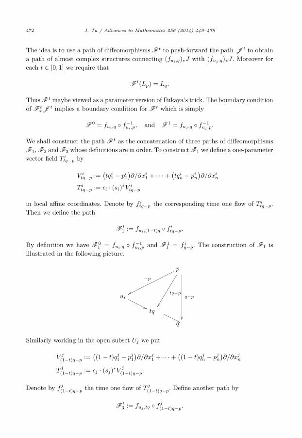
The idea is to use a path of diffeomorphisms F t to push-forward the path J t to obtaina path of almost complex structures connecting (fui,q)∗J with (fuj ,q)∗J . Moreover foreach t ∈ [0, 1] we require that
F t(Lp) = Lq.
Thus F t maybe viewed as a parameter version of Fukaya’s trick. The boundary conditionof F t
∗Jt implies a boundary condition for F t which is simply
F 0 = fui,q ◦ f−1ui,p, and F 1 = fuj ,q ◦ f−1
uj ,p.
We shall construct the path F t as the concatenation of three paths of diffeomorphismsF1, F2 and F3 whose definitions are in order. To construct F1 we define a one-parametervector field T i
tq−p by
V itq−p :=
(tqi1 − pi1
)∂/∂xi
1 + · · · +(tqin − pin
)∂/∂xi
n
T itq−p := εi · (si)∗V i
tq−p
in local affine coordinates. Denote by f itq−p the corresponding time one flow of T i
tq−p.Then we define the path
F t1 := fui,(1−t)q ◦ f i
tq−p.
By definition we have F 01 = fui,q ◦ f−1
ui,p and F 11 = f i
q−p. The construction of F1 isillustrated in the following picture.
ui
q
p
tq
−p
tq−pq−p
Similarly working in the open subset Uj we put
V j(1−t)q−p :=
((1 − t)qj1 − pj1
)∂/∂xj
1 + · · · +((1 − t)qjn − pjn
)∂/∂xj
n
T j(1−t)q−p := εj · (sj)∗V j
(1−t)q−p.
Denote by f j(1−t)q−p the time one flow of T j
(1−t)q−p. Define another path by
F t3 := fuj ,tq ◦ f j .
(1−t)q−p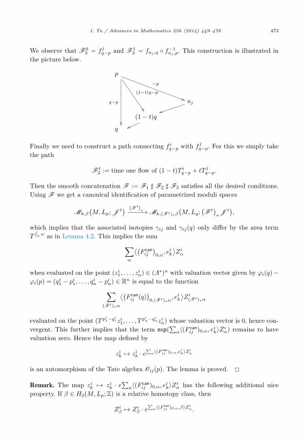
J. Tu / Advances in Mathematics 256 (2014) 449–478 473
We observe that F 03 = f j
q−p and F 13 = fuj ,q ◦ f−1
uj ,p. This construction is illustrated inthe picture below.
uj
q
p
(1 − t)q
−p
(1−t)q−p
q−p
Finally we need to construct a path connecting f iq−p with f j
q−p. For this we simply takethe path
F t2 := time one flow of (1 − t)T i
q−p + tT jq−p.
Then the smooth concatenation F := F1 � F2 � F3 satisfies all the desired conditions.Using F we get a canonical identification of parametrized moduli spaces
Mk,β
(M,Lp; J t
) (F t
)∗−−−−→ Mk,(F t)∗β
(M,Lq;
(F t
)∗J
t),
which implies that the associated isotopies γij and γij(q) only differ by the area termT
∫βω as in Lemma 4.2. This implies the sum∑
α
⟨(F canij
)0,α, e
ik
⟩Ziα
when evaluated on the point (zi1, . . . , zin) ∈ (Λ∗)n with valuation vector given by ϕi(q)−ϕi(p) = (qi1 − pi1, . . . , q
in − pin) ∈ R
n is equal to the function∑(F t)∗α
⟨(F canij (q)
)0,(F t)∗α
, eik⟩Zi
(F t)∗α
evaluated on the point (T pi1−qi1zi1, . . . , T
pin−qinzin) whose valuation vector is 0, hence con-
vergent. This further implies that the term exp(∑
α〈(F canij )0,α, eik〉Zi
α) remains to havevaluation zero. Hence the map defined by
zik �→ zik · e∑
α〈(F canij )0,α,eik〉Zi
α
is an automorphism of the Tate algebra Oij(p). The lemma is proved. �Remark. The map zik �→ zik · e
∑α〈(F can
ij )0,α, eik〉Ziα has the following additional nice
property. If β ∈ H2(M,Lp;Z) is a relative homotopy class, then
Ziβ �→ Zi
β · e∑
α〈(F canij )0,α,β〉Zi
α .
474 J. Tu / Advances in Mathematics 256 (2014) 449–478
This implies that this transformation is compatible with addition of homotopy classes.More precisely if we denote by (Zi
β)∗ = Ziβ · e
∑α〈(F can
ij )0,α,β〉Ziα , then we have
(Ziβ1
)∗ · (Ziβ2
)∗ =(Ziβ1+β2
)∗.
This form of transformation was suggested by Auroux in [1].
4.8. Explicit formula for transition functions
To write down the map Φij in the commutative diagram (4.10) we need also to performan affine change of ordinates since the right vertical exponential map in this diagramwas written in coordinates ϕj rather than ϕi. Thus if the two affine coordinates xi(p) :=(xi
1 − pi1, . . . , xin − pin)t, and xj(p) := (xj
1 − pj1, . . . , xjn − pjn)t transform as
xj(p) = A · xi(p)
for some matrix A = (Akl) ∈ GLn(Z). In terms of exponential coordinates this gives
zjk =∏l
(zil)Akl .
Hence the map Φij can be written down in coordinates by
zjk =∏l
[zil · e
∑α〈(F can
ij )0,α,eil〉Ziα]Akl . (4.11)
Lemma 4.5 ensures the convergence property of Φij (hence well-definedness), andLemma 4.4 ensures the commutativity of diagram (4.10). Finally we define the tran-sition functions Ψij : Spec Oij → Spec Oji by the composition
Ψij : Spec OijSui,p−−−−→ Spec Oij(p)
Φij−−−→ Spec Oji(p)S−1uj,p−−−−→ Spec Oji. (4.12)
Here the maps Sui,p and Suj ,p are defined by formula (4.9).
4.9. Gluing properties of transition functions
Finally we prove that the transition maps defined above satisfy the desired gluingconditions.
Lemma 4.6. We have Ψij ◦ Ψji = id.
Proof. Since Ψij = S−1uj ,pΦijSui,p we have
Ψij ◦ Ψji = S−1u ,pΦijSui,pS
−1u ,pΦjiSuj ,p = S−1
u ,pΦijΦjiSuj ,p.
j i j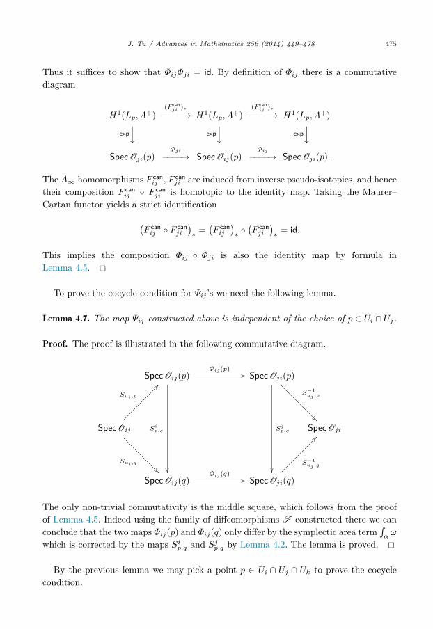
J. Tu / Advances in Mathematics 256 (2014) 449–478 475
Thus it suffices to show that ΦijΦji = id. By definition of Φij there is a commutativediagram
H1(Lp, Λ+)
(F canji )∗
−−−−→ H1(Lp, Λ+)
(F canij )∗
−−−−→ H1(Lp, Λ+)
exp⏐⏐� exp
⏐⏐� exp⏐⏐�
Spec Oji(p)Φji
−−−−→ Spec Oij(p)Φij
−−−−→ Spec Oji(p).
The A∞ homomorphisms F canij , F can
ji are induced from inverse pseudo-isotopies, and hencetheir composition F can
ij ◦ F canji is homotopic to the identity map. Taking the Maurer–
Cartan functor yields a strict identification
(F canij ◦ F can
ji
)∗ =
(F canij
)∗ ◦
(F canji
)∗ = id.
This implies the composition Φij ◦ Φji is also the identity map by formula inLemma 4.5. �
To prove the cocycle condition for Ψij ’s we need the following lemma.
Lemma 4.7. The map Ψij constructed above is independent of the choice of p ∈ Ui ∩ Uj.
Proof. The proof is illustrated in the following commutative diagram.
Spec Oij
Spec Oij(q)
Spec Oij(p)
SpecOji(q)
Spec Oji(p)
Spec Oji
Sui,p
Sui,q
Sip,q
Φij(p)
Φij(q)
Sjp,q
S−1uj,p
S−1uj,q
The only non-trivial commutativity is the middle square, which follows from the proofof Lemma 4.5. Indeed using the family of diffeomorphisms F constructed there we canconclude that the two maps Φij(p) and Φij(q) only differ by the symplectic area term
∫αω
which is corrected by the maps Sip,q and Sj
p,q by Lemma 4.2. The lemma is proved. �By the previous lemma we may pick a point p ∈ Ui ∩ Uj ∩ Uk to prove the cocycle
condition.
476 J. Tu / Advances in Mathematics 256 (2014) 449–478
Lemma 4.8. Let the notations be as above. We have
Ψij(Spec Oij ∩ Spec Oik) ⊂ SpecOji ∩ SpecOjk.
Proof. To prove this we observe that a point (zi1, . . . , zin) ∈ (Λ∗)n is inside Spec Oij ∩Spec Oik if and only if its valuation vector val(zi1, . . . , zin) lies inside ϕi(Uij ∩ Uik). Thenwe have
val(Sui,p
(zi1, . . . , z
in
))=
(val
(zi1)− pi1, . . . , val
(zin
)− pin
);
val(ΦijSui,p
(zi1, . . . , z
in
))=
(∑k
A1k(val
(zik
)− pik
), . . . ,
∑k
Ank
(val
(zik
)− pik
));
val(S−1uj ,pΦijSui,p
(zi1, . . . , z
in
))=
(pj1 +
∑k
A1k(val
(zik
)− pik
), . . . , pjn +
∑k
Ank
(val
(zik
)− pik
)).
Here the matrix A ∈ GLn(Z) is linear part of change of coordinates from xi to xj . Fromthis computation we see that if val(zi1, . . . , zin) ∈ ϕi(Uij ∩Uik) then val(Ψij(zi1, . . . , zin)) ∈ϕj(Ujk ∩ Uji). Thus we have proved the lemma. �Lemma 4.9. The cocycle condition ΨjkΨij = Ψik holds.
Proof. By the construction of Ψ we have
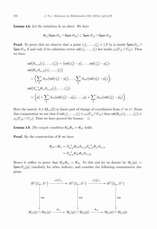
Ψjk ◦ Ψij = S−1uk,p
ΦjkSuj ,pS−1uj ,pΦijSui,p
= S−1uk,p
ΦjkΦijSui,p.
Hence it suffice to prove that ΦjkΦij = Φik. To this end let us denote by Uij(p) :=Spec Oij(p) (similarly for other indices), and consider the following commutative dia-gram.
Uij(p) ∩ Uik(p) Uji(p) ∩ Ujk(p) Uki(p) ∩ Ukj(p)
H1(Lp, Λ+)
H1(Lp, Λ+)
H1(Lp, Λ+)(F can
ij )∗ (F canjk )∗
Φij Φjk
exp exp exp
J. Tu / Advances in Mathematics 256 (2014) 449–478 477
We claim that the top row composition of the above diagram is
(F canjk
)∗ ◦
(F canij
)∗ =
(F canik
)∗.
To see this we use the fact that the space of ω-tamed almost complex structures iscontractible. Hence there exists a two-parameter family of almost complex structuresJx0,x1,x2 ((x0, x1, x2) ∈ Δ2) such that
J0,x1,x2 = Jjk;
Jx0,0,x2 = Jik;
Jx0,x1,0 = Jij .
Here Jij (Jik and Jjk respectively) is the path of almost complex structures usedto construct the homotopy F can
ij (F canik and F can
jk respectively). This two parameterfamily Jx0,x1,x2 induces a 2-homotopy that bounds 1-homotopies γij , γjk and γik.Thus by Theorem 2.7 and homotopy invariance of Maurer–Cartan functor we get(F can
jk )∗◦(F canij )∗ = (F can
ik )∗. To this end we observe there is another commutative diagram
H1(Lp, Λ+)
(F canik )∗
−−−−→ H1(Lp, Λ+)
exp⏐⏐� exp
⏐⏐�Uij(p) ∩ Uik(p)
Φik−−−−→ Uki(p) ∩ Ukj(p).
Combined with the previous diagram, it implies the cocycle condition
ΦjkΦij = Φik
for Φ, which implies that of Ψ . The proof is complete. �It follows from Lemma 4.6, Lemma 4.8 and Lemma 4.9 the local affinoid domains Ui
can be glued to obtain a rigid analytic space which we shall denote by M∨0 . Moreover
the natural valuation maps val : Ui → ϕi(Ui) are compatible with the gluing maps Ψij ,which follows from the computation in the proof of Lemma 4.8. Hence we get a globalvaluation map
val : M∨0 → B0.
This might be thought of as the non-Archimedean version of a torus fibration. We sum-marize the main results of this paper in the following corollary.
Corollary 4.10. Let π : M → B be a Lagrangian torus fibration with vanishing Maslovindex. Assume furthermore Assumption 4.3 holds. Then the local pieces Ui := Spec Oi
478 J. Tu / Advances in Mathematics 256 (2014) 449–478
of affinoid domains can be glued via transition maps Ψij (see formula (4.12)) to form arigid analytic space M∨
0 over the universal Novikov field Λ. Moreover there is a globallydefined valuation map
val : M∨0 → B0.
Acknowledgments
I am grateful to Kenji Fukaya for his encouragement on the subject as well as sharinga slide of his talk at MSRI. I also thank Vadim Vologodsky for useful discussions on non-Archimedean geometry. Finally thanks to the Mathematics Department of University ofOregon for providing excellent research condition.
References
[1] D. Auroux, Mirror symmetry and T-duality in the complement of an anticanonical divisor, J. GökovaGeom. Topol. 1 (2007) 51–91.
[2] S. Bosch, U. Güntzer, R. Remmert, Non-archimedean Analysis, Springer-Verlag, Berlin, 1984.[3] K. Chan, S.-C. Lau, N.C. Leung, SYZ mirror symmetry for toric Calabi–Yau manifolds, J. Differ-
ential Geom. 90 (2) (2012) 177–250.[4] K. Fukaya, Cyclic symmetry and adic convergence in Lagrangian Floer theory, Kyoto J. Math.
50 (3) (2010) 521–590.[5] K. Fukaya, Y.-G. Oh, H. Ohta, K. Ono, Canonical models of filtered A∞-algebras and Morse
complexes, arXiv:0812.1963.[6] K. Fukaya, Y.-G. Oh, H. Ohta, K. Ono, Lagrangian Floer theory on compact toric manifolds I,
Duke Math. J. 151 (2010) 23–174.[7] K. Fukaya, Y.-G. Oh, H. Ohta, K. Ono, Lagrangian Intersection Floer Theory: Anomaly and Ob-
struction, Part I, AMS/IP Studies in Advanced Mathematics, vol. 46.1, American MathematicalSociety/International Press, Providence, RI/Somerville, MA, 2009, xii+396 pp.
[8] E. Getzler, Lie theory for nilpotent L∞-algebras, Ann. of Math. 170 (1) (2009) 271–301.[9] M. Gross, B. Siebert, Mirror symmetry via logarithmic degeneration data, I, J. Differential Geom.
72 (2) (2006) 169–338.[10] M. Gross, B. Siebert, Mirror symmetry via logarithmic degeneration data, II, J. Algebraic Geom.
19 (4) (2010) 679–780.[11] M. Gross, B. Siebert, From real affine geometry to complex geometry, Ann. of Math. (2) 174 (3)
(2011) 1301–1428.[12] V. Hinich, Descent of Deligne groupoids, Int. Math. Res. Not. IMRN (5) (1997) 223–239.[13] M. Kontsevich, Y. Soibelman, Homological mirror symmetry and torus fibrations, in: Symplectic
Geometry and Mirror Symmetry, Seoul, 2000, World Sci. Publ., River Edge, NJ, 2001, pp. 203–263.[14] J. Tu, Homological mirror symmetry is Fourier–Mukai transform, International Mathematics Re-
search Notices, http://dx.doi.org/10.1093/imrn/rnt211.[15] J. Tu, Algebraic structures motivated from family version of Lagrangian Floer theory, in preparation.


![Tropicalcoamoebaandtorus-equivarianthomological ... · in [NU12]. Torus-equivariant homological mirror symmetry for X implies the ordinary homological mirror symmetry, not only for](https://img.pdfslide.us/doc/110x75/60d496ca54cbf835e9608f1d/tropicalcoamoebaandtorus-equivarianthomological-in-nu12-torus-equivariant.jpg)