Embed Size (px)
Citation preview
Journal of Computational Mathematics
Vol.31, No.6, 2013, 573–591.
http://www.global-sci.org/jcm
doi:10.4208/jcm.1309-m3592
ON THE QUASI-RANDOM CHOICE METHOD FOR THELIOUVILLE EQUATION OF GEOMETRICAL OPTICS WITH
DISCONTINUOUS WAVE SPEED*
Jingwei Hu
Institute for Computational Engineering and Sciences (ICES), The University of Texas at Austin,
201 East 24th St, Stop C0200, Austin, TX 78712, USA
Email: [email protected]
Shi Jin
Department of Mathematics, University of Wisconsin-Madison, 480 Lincoln Drive,
Madison, WI 53706, USA
Department of Mathematics, Institute of Natural Sciences, and MOE Key Lab in Scientific and
Engineering Computing, Shanghai Jiao Tong University, Shanghai 200240, China
Email: [email protected]
Abstract
We study the quasi-random choice method (QRCM) for the Liouville equation of ge-
ometrical optics with discontinuous local wave speed. This equation arises in the phase
space computation of high frequency waves through interfaces, where waves undergo partial
transmissions and reflections. The numerical challenges include interface, contact discon-
tinuities, and measure-valued solutions. The so-called QRCM is a random choice method
based on quasi-random sampling (a deterministic alternative to random sampling). The
method not only is viscosity-free but also provides faster convergence rate. Therefore, it
is appealing for the problem under study which is indeed a Hamiltonian flow. Our analy-
sis and computational results show that the QRCM 1) is almost first-order accurate even
with the aforementioned discontinuities; 2) gives sharp resolutions for all discontinuities
encountered in the problem; and 3) for measure-valued solutions, does not need the level
set decomposition for finite difference/volume methods with numerical viscosities.
Mathematics subject classification: 35L45, 65M06, 11K45.
Key words: Liouville equation, High frequency wave, Interface, Measure-valued solution,
Random choice method, Quasi-random sequence.
1. Introduction
In this paper, we study a type of Monte Carlo methods for numerical computation of the
Liouville equation in geometrical optics. Let f(x,v, t) be the energy density distribution of
waves that depends on position x, slowness vector v, and time t, then the Liouville equation
reads
ft +∇vH · ∇xf −∇xH · ∇vf = 0, t > 0, x,v ∈ Rd, (1.1)
where the Hamiltonian H is given by
H(x,v) = c(x)|v| (1.2)
* Received December 23, 2010 / Revised version received July 28, 2013 / Accepted September 16, 2013 /
Published online October 18, 2013 /
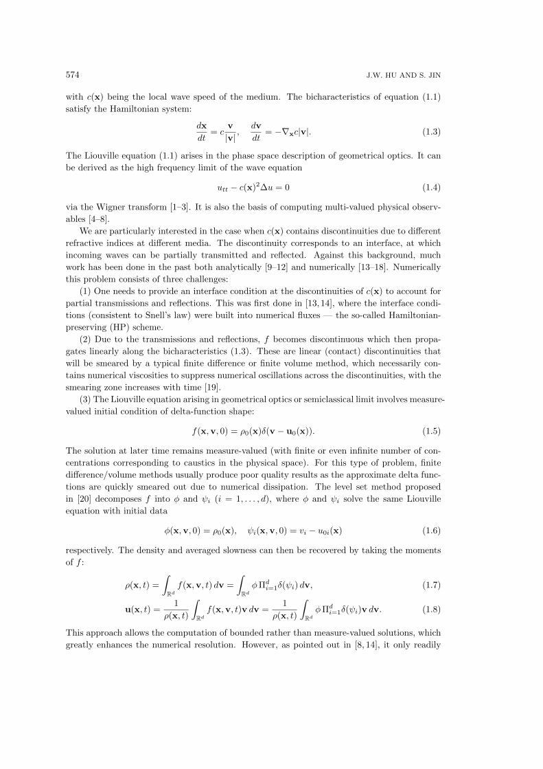
574 J.W. HU AND S. JIN
with c(x) being the local wave speed of the medium. The bicharacteristics of equation (1.1)
satisfy the Hamiltonian system:
dx
dt= c
v
|v|,
dv
dt= −∇xc|v|. (1.3)
The Liouville equation (1.1) arises in the phase space description of geometrical optics. It can
be derived as the high frequency limit of the wave equation
utt − c(x)2∆u = 0 (1.4)
via the Wigner transform [1–3]. It is also the basis of computing multi-valued physical observ-
ables [4–8].
We are particularly interested in the case when c(x) contains discontinuities due to different
refractive indices at different media. The discontinuity corresponds to an interface, at which
incoming waves can be partially transmitted and reflected. Against this background, much
work has been done in the past both analytically [9–12] and numerically [13–18]. Numerically
this problem consists of three challenges:
(1) One needs to provide an interface condition at the discontinuities of c(x) to account for
partial transmissions and reflections. This was first done in [13, 14], where the interface condi-
tions (consistent to Snell’s law) were built into numerical fluxes — the so-called Hamiltonian-
preserving (HP) scheme.
(2) Due to the transmissions and reflections, f becomes discontinuous which then propa-
gates linearly along the bicharacteristics (1.3). These are linear (contact) discontinuities that
will be smeared by a typical finite difference or finite volume method, which necessarily con-
tains numerical viscosities to suppress numerical oscillations across the discontinuities, with the
smearing zone increases with time [19].
(3) The Liouville equation arising in geometrical optics or semiclassical limit involves measure-
valued initial condition of delta-function shape:
f(x,v, 0) = ρ0(x)δ(v − u0(x)). (1.5)
The solution at later time remains measure-valued (with finite or even infinite number of con-
centrations corresponding to caustics in the physical space). For this type of problem, finite
difference/volume methods usually produce poor quality results as the approximate delta func-
tions are quickly smeared out due to numerical dissipation. The level set method proposed
in [20] decomposes f into φ and ψi (i = 1, . . . , d), where φ and ψi solve the same Liouville
equation with initial data
φ(x,v, 0) = ρ0(x), ψi(x,v, 0) = vi − u0i(x) (1.6)
respectively. The density and averaged slowness can then be recovered by taking the moments
of f :
ρ(x, t) =
∫Rd
f(x,v, t) dv =
∫Rd
φΠdi=1δ(ψi) dv, (1.7)
u(x, t) =1
ρ(x, t)
∫Rd
f(x,v, t)v dv =1
ρ(x, t)
∫Rd
φΠdi=1δ(ψi)v dv. (1.8)
This approach allows the computation of bounded rather than measure-valued solutions, which
greatly enhances the numerical resolution. However, as pointed out in [8, 14], it only readily
Quasi-Random Choice Method for Liouville Equation with Discontinuous Wave Speed 575
works for complete transmissions and reflections. For the case of partial transmissions and
reflections, a new level set function has to be added every time the wave hits the interface in
order to track all reflection and refraction branches, thus making the method unfeasible for
multiple interfaces and long computation time. The recent work by Wei et al [18] suggested a
way to handle this problem by the level set method, but it needs an initialization procedure at
every time step.
The random choice method (RCM), or the Glimm’s scheme, was first introduced by Glimm
in 1965 for proving the existence of global weak solutions to hyperbolic system of conservation
laws [21]. Later it was used as a numerical tool by Chorin in gas dynamics [22,23]. Chorin’s work
was followed by numerous researchers, with applications and further improvements in [24–26],
and more recently [27, 28], etc. The main advantage of this method is the sharp resolutions of
shocks and especially, contact discontinuities. In addition, as first investigated by Colella [26], if
the quasi-random sequence rather than random or pseudo-random sequence is used in RCM for
sampling, one can improve the convergence rate from O(1/√N) to O(logN/N)1) . The resulting
RCM which we will call the quasi-random choice method (QRCM) in the sequel, due its lack
of numerical viscosity, seems to be a natural choice to overcome some of the aforementioned
difficulties, since the original Liouville equation is indeed a Hamiltonian (non-dissipative) system
characterized by (1.2).
We would like to mention that the QRCM is restricted to first-order accuracy. The value of
this study is to demonstrate its sharp resolutions for both contact discontinuities and measure-
valued solutions that are typical in high frequency waves through interfaces. Away from singular
regions, higher order methods are more desirable, so it seems to us that a hybrid method that
combines the QRCM with a higher order scheme will offer the best numerical results. Such a
hybrid method is not very difficult to construct as the Liouville equation is linear [29].
The rest of the paper is organized as follows. In the next section, we introduce the original
RCM and extend it to the 2-D linear advection equation that are relevant to solving multi-D
phase space equations. In Section 3, we describe the QRCM and its basic properties (a rigorous
L1-error estimate is given in the appendix for the linear equation with bounded variation
(BV) initial data). In Section 4, a QRCM combined with HP scheme is constructed for the
Liouville equation with discontinuous wave speed. Numerical examples in both 1-D and 2-
D are presented in Section 5 to illustrate the performance of QRCM for discontinuous and
measure-valued solutions.
2. The Random Choice Method
We first describe the original RCM for the 1-D hyperbolic conservation law. There are two
versions of the method in the literature: one uses a staggered grid; the other uses a single grid.
We present the latter here for simplicity.
Consider the initial value problem:
ut + q(u)x = 0, t > 0, x ∈ R, (2.1)
u(x, 0) = u0(x), x ∈ R. (2.2)
Divide the spatial domain into a number of cells[xi− 1
2, xi+ 1
2
)with xi+ 1
2=(i+ 1
2
)h, i ∈ Z.
Each cell is centered at xi = ih of length h. Assume k is the time step size, and define tn = nk,
1) This resembles O(1/√N) and O(logN/N) convergence rates of Monte-Carlo and quasi-Monte Carlo methods
for numerical integration in 1-D.
576 J.W. HU AND S. JIN
n = 0, 1, 2, . . . . Let Un be the approximate solution at time tn which is piecewise constant with
value Uni on the cell[xi− 1
2, xi+ 1
2
). The solution Un+1 at tn+1 is constructed as follows:
Step 1. Solve equation (2.1) accurately with initial data Un. This is equivalent to solve a
Riemann problem on each interval [ih, (i+ 1)h). We impose the CFL condition
‖q′‖L∞(R)k
h≤ 1
2, (2.3)
such that waves from adjacent intervals won’t interact with each other by time tn+1. Define the
exact solution Ue by piecing together all Riemann problem solutions.
Step 2. Choose a random number ξn+1 uniformly distributed on interval [0, 1] and take
Un+1i = Ue
((i− 1
2+ ξn+1
)h, (n+ 1)k
), (2.4)
thus one obtains the approximate solution Un+1.
If the Eq. (2.1) is linear, i.e., q(u) = au, where a is a constant, the above scheme can be
simplified as
for a > 0, Un+1i =
Uni−1 with probability
ak
h,
Uni with probability 1− ak
h;
(2.5)
for a < 0, Un+1i =
Uni+1 with probability − ak
h,
Uni with probability 1 +ak
h.
(2.6)
So in each time step, all function values will either stay there or move a distance h to the
right or left (note that one random number is generated per time step and used for all cells).
Therefore, the RCM has no numerical diffusion and the discontinuity remains perfectly sharp.
Besides, the CFL condition (2.3) can be relaxed to
|a|kh≤ 1, (2.7)
for all the waves travel with the same speed a (they won’t interact at all). Recall that a
first-order upwind scheme for the same equation reads:
for a > 0, Un+1i =
ak
hUni−1 +
(1− ak
h
)Uni ; (2.8)
for a < 0, Un+1i = −ak
hUni+1 +
(1 +
ak
h
)Uni . (2.9)
Hence, unlike the RCM treats Un+1i as a random variable, the finite difference scheme takes
some kind of average — the expected value.
Since the Liouville equation is a linear equation in phase space, what is more relevant in
our context is the following 2-D advection equation
ut + aux + buy = 0, t > 0, x, y ∈ R, (2.10)
u(x, y, 0) = u0(x, y), x, y ∈ R. (2.11)
Quasi-Random Choice Method for Liouville Equation with Discontinuous Wave Speed 577
Let us first write down the upwind scheme for (2.10):
Un+1i,j =
(1− |a|k
h− |b|k
h
)Uni,j +
|a|khUni−sgn(a),j +
|b|khUni,j−sgn(b), (2.12)
where the same discretization is used for both x and y. Analogously to the 1-D case, we can
construct the RCM as follows:
Un+1i =
Uni−sgn(a),j with probability|a|kh,
Uni,j−sgn(b) with probability|b|kh,
Uni,j with probability 1− |a|kh− |b|k
h,
(2.13)
and the CFL condition becomes
|a|kh
+ |b|kh≤ 1. (2.14)
To analyze the numerical error in scheme (2.13), let U0i0,j0
be the initial value of the solution
at (xi0 , yj0), and ηk be the displacement of U0i0,j0
at each time step. Clearly ηk’s are the i.i.d.
random variables that satisfy
P(ηk = (sgn(a)h, 0)) =|a|kh,
P(ηk = (0, sgn(b)h)) =|b|kh,
P(ηk = (0, 0)) = 1− |a|kh− |b|k
h,
(2.15)
where P represents the probability. The expected value and the variance of ηk are then given
by
E[ηk] = (ak, bk), Var[ηk] = (|a|kh− a2k2, |b|kh− b2k2). (2.16)
Suppose after n time steps U0i0,j0
is at (xi0 , yj0) + η, where η =
n∑k=1
ηk is the total displacement.
We have
E[η] =
n∑k=1
E[ηk] = (atn, btn), (2.17)
Var[η] =
n∑k=1
Var[ηk] =
(|a|htn
(1− |a|k
h
), |b|htn
(1− |b|k
h
)). (2.18)
Thus the expected value of η is just the exact displacement. The variance implies that the
location error is of order√htn (assume k/h is constant). Indeed, Lucier [30] showed that the
expected error of RCM in L1(R) at time tn for the 1-D conservation law (2.1) (2.2) is bounded
by (h+
2√3
√h
k
√htn
)‖u0‖BV (R), (2.19)
where ‖u0‖BV (R) is the total variation of u0 on R.
578 J.W. HU AND S. JIN
3. The Quasi-Random Choice Method
In [26], Colella suggested using the quasi-random sequences instead of random or pseudo-
random sequences in the RCM. The quasi-random (also called low-discrepancy) sequence is
purely deterministic: the points in it are correlated to provide greater uniformity [31]. As
a consequence, the resulting RCM (QRCM) can be shown to have a faster convergence rate.
Compared to (2.19), the spatial error is improved from O(√h) to O(|log h|h); the temporal
growth factor is reduced from O(√tn) to O(log tn) (see the appendix for a rigorous proof).
The general idea can be illustrated by a simple example. The argument follows that in [26].
Still consider the 2-D equation (2.10), and as previously let U0i0,j0
be the initial value of the
solution at grid point (xi0 , yj0). We define the location of this value at time tn by
l0 = (xi0 , yj0),
ln =
ln−1 + sgn(a)(h, 0), if ξn ∈
[0,|a|kh
)= I1,
ln−1 + sgn(b)(0, h), if ξn ∈[|a|kh,|a|kh
+|b|kh
)= I2,
ln−1, otherwise,
(3.1)
where ξ = ξ1, ξ2, . . . , ξn, . . . is taken as a quasi-random sequence.
A sequence ξ is said to be equidistributed if for any subinterval I in [0, 1], the proportion of
times that ξj lies in I is asymptotically equal to |I|, the length of I; i.e., if one defines
N{j = 1, . . . , n; ξj ∈ I}n
− |I| = δ(ξ, n, I), (3.2)
then ξ is equidistributed if
Dn = supI⊂[0,1]
|δ(ξ, n, I)| → 0, as n→∞, (3.3)
where Dn is called the discrepancy of the sequence. ξ is said to be quasi-random if
Dn ≤ Clog n
n, (3.4)
in which C is a constant independent of n.
With the above definition, we can express ln in (3.1) as
ln = l0 +N{j = 1, 2, . . . , n; ξj ∈ I1
}· sgn(a)(h, 0)
+N{j = 1, 2, . . . , n; ξj ∈ I2
}· sgn(b)(0, h)
= l0 +
(ak
h+ sgn(a)δ(ξ, n, I1)
)(nh, 0) +
(bk
h+ sgn(b)δ(ξ, n, I2)
)(0, nh)
= l0 + (atn, btn) +h
ktn(sgn(a)δ(ξ, n, I1), sgn(b)δ(ξ, n, I2)). (3.5)
Therefore, the error between ln and the exact location l0 + (atn, btn) is bounded by
C1h
ktn
log n
n, (3.6)
which goes to zero as n → ∞, when tn and h/k fixed. Furthermore, since n = O(1/h), this
error is of order O(|log h|h), better than O(√h) of the random sequence based RCM.
Quasi-Random Choice Method for Liouville Equation with Discontinuous Wave Speed 579
The simplest example of a quasi-random sequence is the van der Corput sequence [32]. It is
constructed by reversing the base b representation of the sequence of natural numbers. In the
binary case (b = 2), let
n =
m∑k=0
ik2k, ik = 0, 1 (3.7)
be the binary expansion of n = 1, 2, . . . , then
ξn =
m∑k=0
ik2−(k+1). (3.8)
We will use this sequence in our numerical simulation.
Remark 3.1. The quasi-random sequences applied to Monte-Carlo integration is a popular
research topic in mathematical finance. The in-depth study of their properties is beyond the
scope of the paper. A nice review can be found in [33].
4. A Quasi-Random Choice Scheme for the Liouville Equation with
Discontinuous Wave Speed
In this section, we present the numerical scheme for the Liouville equation (1.1), which is
a combination of the QRCM and the HP scheme [14]. For discontinuous wave speed c(x), the
combined method not only captures the correct physics (attributed to HP scheme) but also
provides sharp resolutions at contact discontinuities induced by the interface (attributed to
QRCM). For generality, the scheme will be given for the 2-D case (2-D for both spatial and
slowness domain). Simplification to 1-D and extension to 3-D are straightforward.
Consider the 2-D Liouville equation:
ft +c(x, y)u√u2 + v2
fx +c(x, y)v√u2 + v2
fy − cx√u2 + v2fu − cy
√u2 + v2fv = 0. (4.1)
Assume a uniform mesh for all directions x, y, u, v: the phase space is divided into a number
of cells with boundaries at xi+ 12, yj+ 1
2, uk+ 1
2, vl+ 1
2, and the cells are centered at (xi, yj , uk, vl)
with sidelength h. The time domain is discretized as before: tn = nk with step size k. We
approximate c(x, y) by a piecewise bilinear function, and always provide two interface values at
each cell interface, e.g., c−i+ 1
2 ,jand c+
i+ 12 ,j
at xi+ 12 ,j
, when c is smooth at xi+ 12 ,j
, the two values
are identical. Therefore, the derivatives cx and cy in the cell (i, j, k, l) can be approximated by
cx ≈c−i+ 1
2 ,j− c+
i− 12 ,j
h, cy ≈
c−i,j+ 1
2
− c+i,j− 1
2
h. (4.2)
Since the interfaces lie in the spatial domain, the main difficulty of solving (4.1) comes from the
transport terms in the (x, y) plane. To simplify the problem, in what follows, we will assume
the wave speed c as a piecewise constant function, so the equation (4.1) becomes
ft +c(x, y)u√u2 + v2
fx +c(x, y)v√u2 + v2
fy = 0. (4.3)
The combined QRCM and HP scheme for (4.3) when c(x,y)u√u2+v2
> 0 and c(x,y)v√u2+v2
< 0 is given in
Algorithm 4.1 (other cases are treated similarly).
580 J.W. HU AND S. JIN
Algorithm 4.1 The combined QRCM and HP scheme for the 2-D Liouville equation (4.3).
1: for each tn+1 do
2: fetch a new quasi-random number ξn+1 from the van der Corput sequence;
3: for each xi, yj , uk, vl do
4: ai,j = ci,juk√u2k+v
2l
; bi,j = ci,jvl√u2k+v
2l
;
5: if ξn+1 <ai,jkh then
6: if at the cell (i, j, k, l) right to the interface (xi− 12, yj) then
7: uR = −uk;
8: if w =
(c+i− 1
2,j
c−i− 1
2,j
)2
u2k +
( c+i− 1
2,j
c−i− 1
2,j
)2
− 1
v2l > 0 then
9: uT =√w; find index m such that um−1 < uT < um;
10: γin = uT√u2T+v2l
; γtr = uk√u2k+v
2l
; αR =
(c+i− 1
2,jγin−c−
i− 12,jγtr
c+i− 1
2,jγin+c−
i− 12,jγtr
)2
; αT = 1− αR;
11: fn+1i,j,k,l = αT
(um−uT
h fni−1,j,m−1,l + uT−um−1
h fni−1,j,m,l
)+ αRfni,j,R,l;
12: else
13: fn+1i,j,k,l = fni,j,R,l;
14: end if
15: else
16: fn+1i,j,k,l = fni−1,j,k,l;
17: end if
18: else ifai,jkh < ξn+1 <
ai,jkh − bi,jk
h then
19: if at the cell (i, j, k, l) down to the interface (xi, yj+ 12) then
20: vR = −vl;
21: if w =
( c−i,j+1
2
c+i,j+1
2
)2
− 1
u2k +
(c−i,j+1
2
c+i,j+1
2
)2
v2l > 0 then
22: vT = −√w; find index m such that vm−1 < vT < vm;
23: γin = −vT√u2k+v
2T
; γtr = −vl√u2k+v
2l
; αR =
(c−i,j+1
2
γin−c+i,j+1
2
γtr
c−i,j+1
2
γin−c+i,j+1
2
γtr
)2
; αT = 1− αR;
24: fn+1i,j,k,l = αT
(vm−vT
h fni,j+1,k,m−1 + vT−vm−1
h fni,j+1,k,m
)+ αRfni,j,k,R;
25: else
26: fn+1i,j,k,l = fni,j,k,R;
27: end if
28: else
29: fn+1i,j,k,l = fni,j+1,k,l;
30: end if
31: else
32: fn+1i,j,k,l = fni,j,k,l;
33: end if
34: end for
35: end for
5. Numerical Examples
In this section, we study the numerical performance of the algorithm in section 4 for the
Liouville equation with discontinuous wave speed. The emphasis is given to measure-valued
Quasi-Random Choice Method for Liouville Equation with Discontinuous Wave Speed 581
solutions with partial transmissions and reflections at the interface. As mentioned in the intro-
duction, the level set decomposing approach [20] does not work in this case, so a finite differ-
ence/volume method that directly evolves the approximate delta function is expected to have
poor resolutions. We will show, however, the QRCM performs equally well for both bounded
and measure-valued solutions, hence no special treatment of the delta function is needed.
Three different methods will be compared in the following: the first-order upwind scheme
(referred to as upwind), the second-order Lax-Wendroff scheme with the van Leer flux limiter
(referred to as LW-lim) [34], and the QRCM based on base 2 van der Corput sequence.
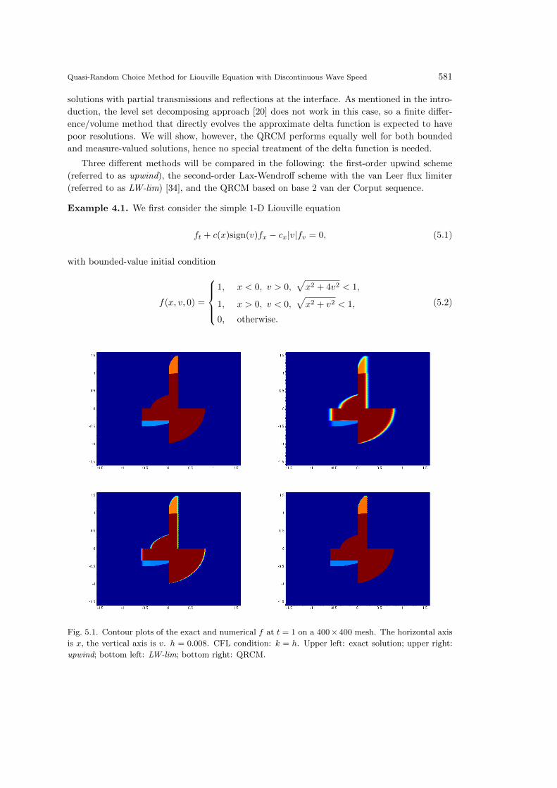
Example 4.1. We first consider the simple 1-D Liouville equation
ft + c(x)sign(v)fx − cx|v|fv = 0, (5.1)
with bounded-value initial condition
f(x, v, 0) =
1, x < 0, v > 0,
√x2 + 4v2 < 1,
1, x > 0, v < 0,√x2 + v2 < 1,
0, otherwise.
(5.2)
Fig. 5.1. Contour plots of the exact and numerical f at t = 1 on a 400× 400 mesh. The horizontal axis
is x, the vertical axis is v. h = 0.008. CFL condition: k = h. Upper left: exact solution; upper right:
upwind; bottom left: LW-lim; bottom right: QRCM.
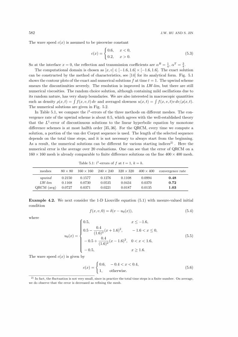
582 J.W. HU AND S. JIN
The wave speed c(x) is assumed to be piecewise constant
c(x) =
{0.6, x < 0,
0.2, x > 0.(5.3)
So at the interface x = 0, the reflection and transmission coefficients are αR = 14 , αT = 3
4 .
The computational domain is chosen as [x, v] ∈ [−1.6, 1.6]× [−1.6, 1.6]. The exact solution
can be constructed by the method of characteristics, see [14] for its analytical form. Fig. 5.1
shows the contour plots of the exact and numerical solutions f at time t = 1. The upwind scheme
smears the discontinuities severely. The resolution is improved in LW-lim, but there are still
numerical viscosities. The random choice solution, although containing mild oscillations due to
its random nature, has very sharp boundaries. We are also interested in macroscopic quantities
such as density ρ(x, t) =∫f(x, v, t) dv and averaged slowness u(x, t) =
∫f(x, v, t)v dv/ρ(x, t).
The numerical solutions are given in Fig. 5.2.
In Table 5.1, we compare the l1-errors of the three methods on different meshes. The con-
vergence rate of the upwind scheme is about 0.5, which agrees with the well-established theory
that the L1-error of discontinuous solutions to the linear hyperbolic equation by monotone
difference schemes is at most halfth order [35, 36]. For the QRCM, every time we compute a
solution, a portion of the van der Corput sequence is used. The length of the selected sequence
depends on the total time steps, and it is not necessary to always start from the beginning.
As a result, the numerical solutions can be different for various starting indices2) . Here the
numerical error is the average over 20 evaluations. One can see that the error of QRCM on a
160× 160 mesh is already comparable to finite difference solutions on the fine 400× 400 mesh.
Table 5.1: l1-errors of f at t = 1, k = h.
meshes 80× 80 160× 160 240× 240 320× 320 400× 400 convergence rate
upwind 0.2150 0.1577 0.1276 0.1108 0.0994 0.48
LW-lim 0.1168 0.0730 0.0535 0.0434 0.0370 0.72
QRCM (avg) 0.0727 0.0371 0.0221 0.0187 0.0135 1.03
Example 4.2. We next consider the 1-D Liouville equation (5.1) with mesure-valued initial
condition
f(x, v, 0) = δ(v − u0(x)), (5.4)
where
u0(x) =
0.5, x ≤ −1.6,
0.5− 0.4
(1.6)2(x+ 1.6)2, − 1.6 < x ≤ 0,
− 0.5 +0.4
(1.6)2(x− 1.6)2, 0 < x < 1.6,
− 0.5, x ≥ 1.6.
(5.5)
The wave speed c(x) is given by
c(x) =
{0.6, − 0.4 < x < 0.4,
1, otherwise.(5.6)
2) In fact, the fluctuation is not very small, since in practice the total time steps is a finite number. On average,
we do observe that the error is decreased as refining the mesh.
Quasi-Random Choice Method for Liouville Equation with Discontinuous Wave Speed 583
−1.5 −1 −0.5 0 0.5 1 1.5−0.5
0
0.5
1
1.5
2
2.5
−0.4 −0.2 0 0.2 0.4 0.6−0.5
−0.4
−0.3
−0.2
−0.1
0
0.1
0.2
0.3
−1.5 −1 −0.5 0 0.5 1 1.5−0.5
0
0.5
1
1.5
2
2.5
−0.4 −0.2 0 0.2 0.4 0.6−0.5
−0.4
−0.3
−0.2
−0.1
0
0.1
0.2
0.3
−1.5 −1 −0.5 0 0.5 1 1.5−0.5
0
0.5
1
1.5
2
2.5
−0.4 −0.2 0 0.2 0.4 0.6−0.5
−0.4
−0.3
−0.2
−0.1
0
0.1
0.2
0.3
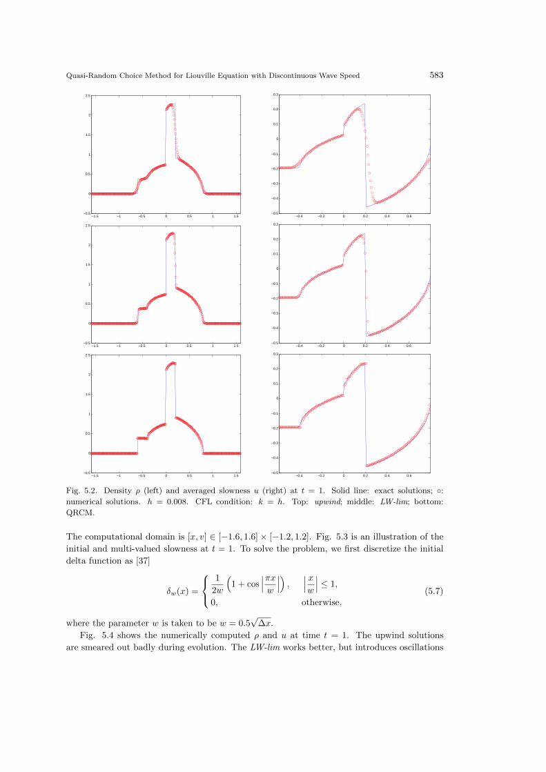
Fig. 5.2. Density ρ (left) and averaged slowness u (right) at t = 1. Solid line: exact solutions; ◦:numerical solutions. h = 0.008. CFL condition: k = h. Top: upwind; middle: LW-lim; bottom:
QRCM.
The computational domain is [x, v] ∈ [−1.6, 1.6]× [−1.2, 1.2]. Fig. 5.3 is an illustration of the
initial and multi-valued slowness at t = 1. To solve the problem, we first discretize the initial
delta function as [37]
δw(x) =
1
2w
(1 + cos
∣∣∣πxw
∣∣∣) , ∣∣∣ xw
∣∣∣ ≤ 1,
0, otherwise,(5.7)
where the parameter w is taken to be w = 0.5√
∆x.
Fig. 5.4 shows the numerically computed ρ and u at time t = 1. The upwind solutions
are smeared out badly during evolution. The LW-lim works better, but introduces oscillations
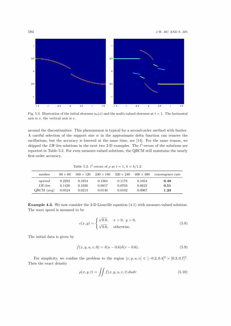
584 J.W. HU AND S. JIN
Fig. 5.3. Illustration of the initial slowness u0(x) and the multi-valued slowness at t = 1. The horizontal
axis is x, the vertical axis is v.
around the discontinuities. This phenomenon is typical for a second-order method with limiter.
A careful selection of the support size w in the approximate delta function can remove the
oscillations, but the accuracy is lowered at the same time, see [14]. For the same reason, we
skipped the LW-lim solutions in the next two 2-D examples. The l1-errors of the solutions are
reported in Table 5.2. For even measure-valued solutions, the QRCM still maintains the nearly
first-order accuracy.
Table 5.2: l1-errors of ρ at t = 1, k = h/1.2.
meshes 80× 60 160× 120 240× 180 320× 240 400× 300 convergence rate
upwind 0.2282 0.1654 0.1364 0.1178 0.1054 0.48
LW-lim 0.1420 0.1026 0.0817 0.0703 0.0622 0.51
QRCM (avg) 0.0524 0.0213 0.0140 0.0102 0.0067 1.23
Example 4.3. We now consider the 2-D Liouville equation (4.1) with measure-valued solution.
The wave speed is assumed to be
c(x, y) =
{√0.8, x > 0, y > 0,√
0.6, otherwise.(5.8)
The initial data is given by
f(x, y, u, v, 0) = δ(u− 0.6)δ(v − 0.6). (5.9)
For simplicity, we confine the problem to the region [x, y, u, v] ∈ [−0.2, 0.4]2 × [0.3, 0.7]2.
Then the exact density
ρ(x, y, t) =
∫∫f(x, y, u, v, t) dudv (5.10)
Quasi-Random Choice Method for Liouville Equation with Discontinuous Wave Speed 585
−1.5 −1 −0.5 0 0.5 1 1.50.5
1
1.5
2
2.5
3
3.5
−1.5 −1 −0.5 0 0.5 1 1.5
−0.5
−0.4
−0.3
−0.2
−0.1
0
0.1
0.2
0.3
0.4
0.5
−1.5 −1 −0.5 0 0.5 1 1.50.5
1
1.5
2
2.5
3
3.5
−1.5 −1 −0.5 0 0.5 1 1.5
−0.5
−0.4
−0.3
−0.2
−0.1
0
0.1
0.2
0.3
0.4
0.5
−1.5 −1 −0.5 0 0.5 1 1.50.5
1
1.5
2
2.5
3
3.5
−1.5 −1 −0.5 0 0.5 1 1.5
−0.5
−0.4
−0.3
−0.2
−0.1
0
0.1
0.2
0.3
0.4
0.5
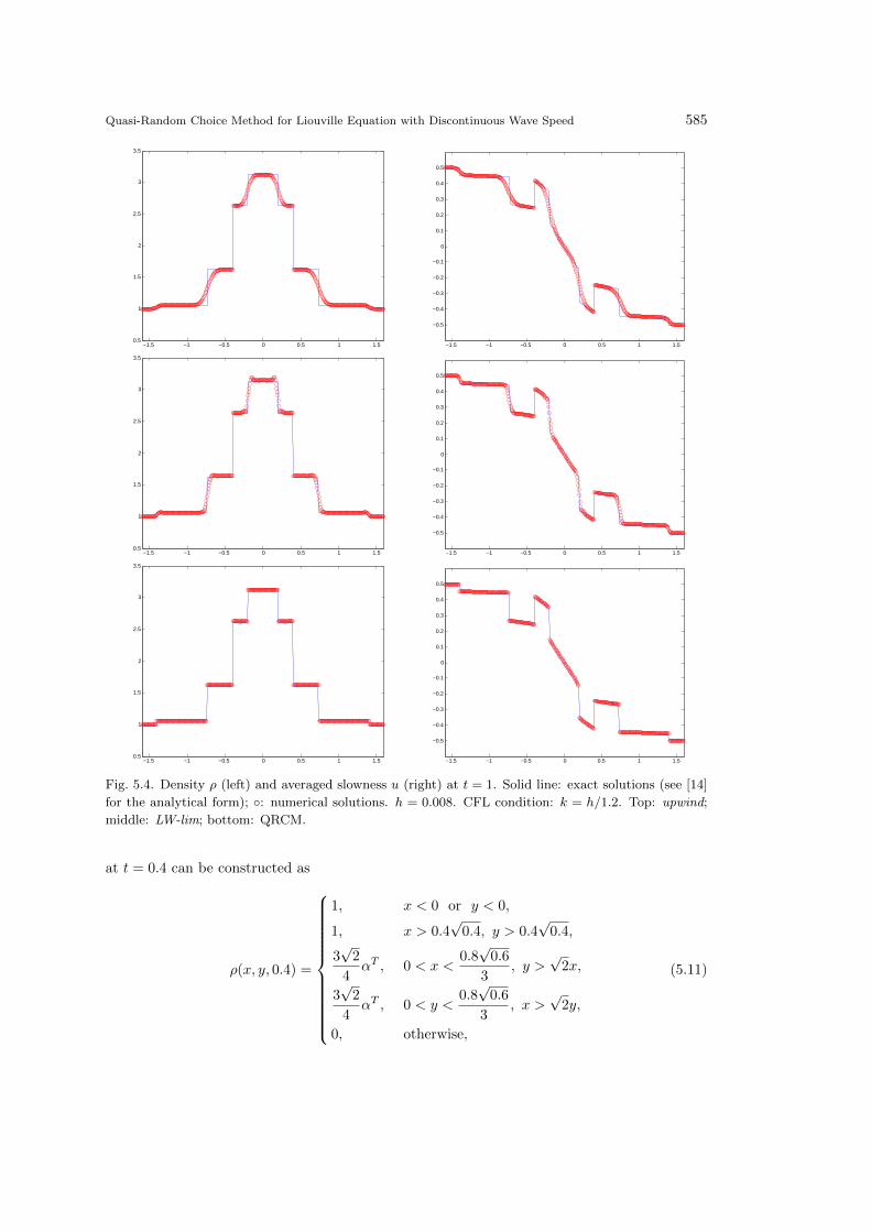
Fig. 5.4. Density ρ (left) and averaged slowness u (right) at t = 1. Solid line: exact solutions (see [14]
for the analytical form); ◦: numerical solutions. h = 0.008. CFL condition: k = h/1.2. Top: upwind;
middle: LW-lim; bottom: QRCM.
at t = 0.4 can be constructed as
ρ(x, y, 0.4) =
1, x < 0 or y < 0,
1, x > 0.4√
0.4, y > 0.4√
0.4,
3√
2
4αT , 0 < x <
0.8√
0.6
3, y >
√2x,
3√
2
4αT , 0 < y <
0.8√
0.6
3, x >
√2y,
0, otherwise,
(5.11)
586 J.W. HU AND S. JIN
where αR =(√
2−1√2+1
)2, αT = 1− αR.
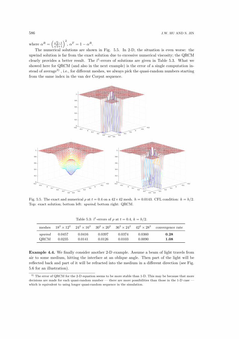
The numerical solutions are shown in Fig. 5.5. In 2-D, the situation is even worse: the
upwind solution is far from the exact solution due to excessive numerical viscosity; the QRCM
clearly provides a better result. The l1-errors of solutions are given in Table 5.3. What we
showed here for QRCM (and also in the next example) is the error of a single computation in-
stead of average3) , i.e., for different meshes, we always pick the quasi-random numbers starting
from the same index in the van der Corput sequence.
−0.2−0.1
00.1
0.20.3
0.4
−0.2−0.1
00.1
0.20.3
0.4
0
0.2
0.4
0.6
0.8
1
−0.2−0.1
00.1
0.20.3
0.4
−0.2−0.1
00.1
0.20.3
0.4
0
0.2
0.4
0.6
0.8
1
−0.2−0.1
00.1
0.20.3
0.4
−0.2−0.1
00.1
0.20.3
0.4
0
0.2
0.4
0.6
0.8
1
Fig. 5.5. The exact and numerical ρ at t = 0.4 on a 42×42 mesh. h = 0.0143. CFL condition: k = h/2.
Top: exact solution; bottom left: upwind; bottom right: QRCM.
Table 5.3: l1-errors of ρ at t = 0.4, k = h/2.
meshes 182 × 122 242 × 162 302 × 202 362 × 242 422 × 282 convergence rate
upwind 0.0457 0.0416 0.0397 0.0374 0.0360 0.28
QRCM 0.0235 0.0141 0.0126 0.0103 0.0090 1.08
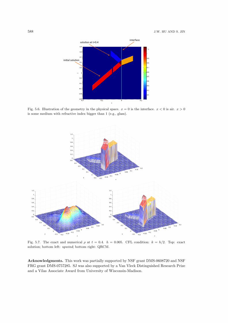
Example 4.4. We finally consider another 2-D example. Assume a beam of light travels from
air to some medium, hitting the interface at an oblique angle. Then part of the light will be
reflected back and part of it will be refracted into the medium in a different direction (see Fig.
5.6 for an illustration).
3) The error of QRCM for the 2-D equation seems to be more stable than 1-D. This may be because that more
decisions are made for each quasi-random number — there are more possibilities than those in the 1-D case —
which is equivalent to using longer quasi-random sequence in the simulation.
Quasi-Random Choice Method for Liouville Equation with Discontinuous Wave Speed 587
The problem can formulated mathematically as follows: let the wave speed be
c(x, y) =
{cl, x < 0,
cr, x > 0,(5.12)
with cl = 1, cr = 2/3. The initial condition is given by
f(x, y, u, v, 0) = ρ0(x, y)δ(u− u0)δ(v − v0), (5.13)
where u0 = 1, v0 = 1.6, and
ρ0(x, y) =
{1, |y − v0x/u0 − 0.2| < 0.05, −0.3 < x < −0.1,
0, otherwise.(5.14)
The exact density ρ(x, y, t) at t = 0.4 is given by
ρ(x, y, 0.4)
= Ireg1 · ρ0
(x− 0.4cru0√
u20 + v20, y − 0.4crv0√
u20 + v20
)+ Ireg2 · ρ0
(x− 0.4u0√
u20 + v20, y − 0.4v0√
u20 + v20
)
+ Ireg3 · αRρ0
(−x− 0.4u0√
u20 + v20, y − 0.4v0√
u20 + v20
)+ Ireg4 · αT
u0
cr√u20 + (1− c2r)v20
· ρ0
(u0x
cr√u20 + (1− c2r)v20
− 0.4u0√u20 + v20
, y − 0.4v0√u20 + v20
+(1− c2r)v0x
cr√u20 + (1− c2r)v20
), (5.15)
where
Ireg1 =
{(x, y) : x >
0.4cru0√u20 + v20
}, Ireg2 = {(x, y) : x < 0} ,
Ireg3 =
{(x, y) : − 0.4u0√
u20 + v20< x < 0
},
Ireg4 =
{(x, y) : 0 < x <
0.4cr√u20 + (1− c2r)v20√u20 + v20
},
αR =
(cru0 −
√u20 + (1− c2r)v20
cru0 +√u20 + (1− c2r)v20
)2
, αT = 1− αR.
(5.16)
Our computational domain is chosen as x ∈ [−0.4, 0.2], y ∈ [−0.5, 0.5], u ∈ [−1.1,−0.9] ∪[0.9, 1.1] ∪ [2.25, 2.45], v ∈ [1.5, 1.7] (the domain for u, v is chosen adaptively to minimize the
computational cost). The numerical results and the l1-errors are shown in Fig. 5.7 and Table
5.4 respectively. For this relatively large problem, one can barely see the shape of the exact
solution for the upwind method, whereas the QRCM basically captures the correct shape and
amplitude of the exact solution.
Table 5.4: l1-errors of ρ at t = 0.4, k = h/2.
h 0.04 0.02 0.01 0.005 convergence rate
upwind 0.0332 0.0275 0.0244 0.0198 0.24
QRCM 0.0171 0.0114 0.0044 0.0030 0.89
588 J.W. HU AND S. JIN
ini#al solu#on
solu#on at t=0.4 interface
Fig. 5.6. Illustration of the geometry in the physical space. x = 0 is the interface. x < 0 is air. x > 0
is some medium with refractive index bigger than 1 (e.g., glass).
−0.2−0.15
−0.1−0.05
00.05
0.10.15
0.2
−0.1
0
0.1
0.2
0.3
0.4
0.5
0
0.2
0.4
0.6
0.8
1
1.2
xy
−0.2−0.15
−0.1−0.05
00.05
0.10.15
0.2
−0.1
0
0.1
0.2
0.3
0.4
0.5
0
0.2
0.4
0.6
0.8
1
1.2
xy −0.2
−0.15−0.1
−0.050
0.050.1
0.150.2
−0.1
0
0.1
0.2
0.3
0.4
0.5
0
0.2
0.4
0.6
0.8
1
1.2
xy
Fig. 5.7. The exact and numerical ρ at t = 0.4. h = 0.005. CFL condition: k = h/2. Top: exact
solution; bottom left: upwind; bottom right: QRCM.
Acknowledgments. This work was partially supported by NSF grant DMS-0608720 and NSF
FRG grant DMS-0757285. SJ was also supported by a Van Vleck Distinguished Research Prize
and a Vilas Associate Award from University of Wisconsin-Madison.
Quasi-Random Choice Method for Liouville Equation with Discontinuous Wave Speed 589
Appendix A. The L1-error estimate of the quasi-random choice
method for the linear equation
In this appendix, we prove rigorously the L1-error estimate of the QRCM for the linear
equation:
ut + aux = 0, x ∈ R, t > 0, a > 0, (A.1)
u(x, 0) = u0(x), x ∈ R. (A.2)
We assume that the initial data u0 has bounded variation on R, i.e.,
‖u0‖BV (R) = sup
N∑j=1
|u0(xj)− u0(xj−1)| <∞, (A.3)
where the supremum is taken over all subdivisions of the real line −∞ = x0 < x1 < · · · < xN =
∞. Some techniques used here are similar to those in [38]. We have the following:
Theorem A.1. Let u(x, t) be the exact solution of (A.1) (A.2), and Un(x, t) be the piecewise
constant solution at tn obtained by the QRCM, then
‖u(·, tn)−Un(·, tn)‖L1(R) ≤[C1 log
(h
ktn
)h+ C2 |log h|h
]‖u0‖BV (R). (A.4)
Proof. Let v(x, t) be the exact solution of (A.1) with initial data U0(x, 0) (the piecewise
constant approximation of u0), then
‖u(·, tn)−Un(·, tn)‖L1(R) ≤ ‖u(·, tn)− v(·, tn)‖L1(R) + ‖v(·, tn)−Un(·, tn)‖L1(R). (A.5)
Since equation (A.1) is linear, the first term on the right hand side of (A.5) can be bounded by
‖u(·, tn)− v(·, tn)‖L1(R) ≤ ‖u0(·)−U0(·, 0)‖L1(R) ≤ h‖u0‖BV (R). (A.6)
To estimate the second term ‖v(·, tn)−Un(·, tn)‖L1(R), we decompose the initial data U0(x, 0)
in the following way:
U0(x, 0) =
∞∑i=−∞
wi(x), (A.7)
where
wi(x) =
0, x <
(i+
1
2
)h,
U0i+1 − U0
i , x >
(i+
1
2
)h.
(A.8)
Let vwi(x, t), Un
wi(x, t) denote respectively the exact and the QRCM solutions with initial data
wi(x), then
‖v(·, tn)−Un(·, tn)‖L1(R) =
∥∥∥∥∥∞∑
i=−∞
[vwi
(·, tn)−Unwi
(·, tn)]∥∥∥∥∥L1(R)
≤∞∑
i=−∞‖vwi
(·, tn)−Unwi
(·, tn)‖L1(R). (A.9)
590 J.W. HU AND S. JIN
Assume the same quasi-random sequence is used for all wi. From the discussion in Section 3,
we know
‖vwi(·, tn)−Un
wi(·, tn)‖L1(R) ≤
h
ktn |δ(ξ, n, I)|
∣∣U0i+1 − U0
i
∣∣ , (A.10)
where I = [0, ak/h). Therefore,
‖v(·, tn)−Un(·, tn)‖L1(R) ≤h
ktn |δ(ξ, n, I)|
∞∑i=−∞
∣∣U0i+1 − U0
i
∣∣≤ h
ktn |δ(ξ, n, I)| ‖u0‖BV (R)
≤ Chktn
log n
n‖u0‖BV (R). (A.11)
To sum up
‖u(·, tn)−Un(·, tn)‖L1(R) ≤ h‖u0‖BV (R) + Ch
ktn
log n
n‖u0‖BV (R)
≤[h+ C log
(h
k
tnh
)h
]‖u0‖BV (R)
≤[C1 log
(h
ktn
)h+ C2 |log h|h
]‖u0‖BV (R). (A.12)
References
[1] P.L. Lions and T. Paul, Sur les mesures de Wigner, Rev. Math. Iberoamericana, 9 (1993), 553–618.
[2] L. Ryzhik, G. Papanicolaou and J.B. Keller, Transport equations for elastic and other waves in
random media, Wave Motion, 24 (1996), 327–370.
[3] P. Gerard, P.A. Markowich, N.J. Mauser and F. Poupaud, Homogenization limits and Wigner
transforms, Commun. Pure Appl. Math., 50 (1997), 323–379.
[4] B. Engquist, O. Runborg and A.K. Tornberg, High-frequency wave propagation by the segment
projection method, J. Comput. Phys., 178 (2002), 373–390.
[5] S. Fomel and J.A. Sethian, Fast-phase space computation of multiple arrivals, Proc. Nat. Acad.
Sci. U.S.A., 99 (2002), 7329–7334.
[6] S. Jin and S. Osher, A level set method for the computation of multivalued solutions to quasi-linear
hyperbolic PDEs and Hamilton-Jacobi equations, Comm. Math. Sci., 1 (2003), 575–591.
[7] B. Engquist and O. Runborg, Computational high frequency wave propagation, Acta Numerica,
12 (2003), 181–266.
[8] L.T. Cheng, M. Kang, S. Osher, H. Shim and Y.H. Tsai, Reflection in a level set framework for
geometric optics, Comput. Model. Eng. Sci., 5 (2004), 347–360.
[9] F. Nier, Asymptotic analysis of a scaled Wigner equation and quantum scattering, Transp. Theory
Stat. Phys., 24 (1995), 591–629.
[10] F. Nier, A semi-classical picture of quantum scattering, Ann. Sci. Ec. Norm. Sup., 29 (1996),
149–183.
[11] G. Bal, J.B. Keller, G. Papanicolaou and L. Ryzhik, Transport theory for acoustic waves with
reflection and transmission at interfaces, Wave Motion, 30 (1999), 303–327.
[12] L. Miller, Refraction of high frequency waves density by sharp interfaces and semiclassical measures
at the boundary, J. Math. Pures Appl., 79 (2000), 227–269.
[13] S. Jin and X. Wen, Hamiltonian-preserving schemes for the Liouville equation of geometrical
optics with discontinuous local wave speeds, J. Comput. Phys., 214 (2006), 672–697.
Quasi-Random Choice Method for Liouville Equation with Discontinuous Wave Speed 591
[14] S. Jin and X. Wen, A Hamiltonian-preserving scheme for the Liouville equation of geometrical
optics with partial transmissions and reflections, SIAM J. Numer. Anal., 44 (2006), 1801–1828.
[15] S. Jin and K.A. Novak, A semiclassical transport model for thin quantum barriers, Multiscale
Model. Simul., 5 (2006), 1063–1086.
[16] S. Jin, H. Wu and Z. Huang, A hybrid phase-flow method for Hamiltonian systems with discon-
tinuous Hamiltonians, SIAM J. Sci. Comput., 31 (2008), 1303–1321.
[17] S. Jin and K.A. Novak, A coherent semiclassical transport model for pure-state quantum scatter-
ing, Comm. Math. Sci., 8 (2010), 253–275.
[18] D. Wei, S. Jin, R. Tsai and X. Yang, A level set method for the semiclassical limit of the
Schrodinger equation with discontinuous potentials, J. Comput. Phys., 229 (2010), 7440–7455.
[19] A. Harten, The artificial compression method for computation of shocks and contact discontinu-
ities. I. Single conservation laws, Commun. Pure Appl. Math., 30 (1977), 611–638.
[20] S. Jin, H. Liu, S. Osher and R. Tsai, Computing multi-valued physical observables for the high
frequency limit of symmetric hyperbolic systems, J. Comput. Phys., 210 (2005), 497–518.
[21] J. Glimm, Solutions in the large for nonlinear hyperbolic systems of equations, Commun. Pure
Appl. Math., 18 (1965), 697–715.
[22] A.J. Chorin, Random choice solution of hyperbolic systems, J. Comput. Phys., 22 (1976), 517–533.
[23] A.J. Chorin, Random choice methods with applications to reacting gas flow, J. Comput. Phys.,
25 (1977), 253–272.
[24] G.A. Sod, A numerical study of a coverging cylindrical shock, J. Fluid Mech., 83 (1977), 785–794.
[25] P. Concus and W. Proskurowski, Numerical solution of a nonlinear hyperbolic equation by the
random choice method, J. Comput. Phys., 30 (1979), 153–166.
[26] P. Colella, Glimm’s method for gas dynamics, SIAM J. Sci. Stat. Comput., 3 (1982), 76–110.
[27] C.Y. Loh, M.S. Liou and W.H. Hui, An investigation of random choice method for three-
dimensional steady supersonic flows, Int. J. Numer. Methods Fluids, 29 (1999), 97–119.
[28] A. Jazcilevich and V. Fuentes-Gea, The conservative random choice method for the numerical
solution of the advection equation, Monthly Weather Review, 127 (1999), 2281–2292.
[29] X. Wen, A high order numerical method for computing physical observables in the semiclassical
limit of the one dimensional linear Schrodinger equation with discontinuous potentials, J. Sci.
Comput., 42 (2010), 318–344.
[30] B.J. Lucier, Error bounds for the methods of Glimm, Godunov and LeVeque, SIAM J. Numer.
Anal., 22 (1985), 1074–1081.
[31] H. Niederreiter, Random Number Generation and Quasi-Monte Carlo Methods, SIAM, Philadel-
phia, PA, 1992.
[32] J.G.van der Corput, Verteilungsfunktionen, Proc. Ned. Akad. v. Wet., 38 (1935), 813–821.
[33] R.E. Caflisch, Monte Carlo and quasi-Monte Carlo methods, Acta Numerica, (1998), 1–49.
[34] R.J. LeVeque, Numerical Methods for Conservation Laws, Birkhauser Verlag, Basel, second
edition, 1992.
[35] N.N. Kuznetsov, Accuracy of some approximate methods for computing the weak solutions of a
first-order quasi-linear equation, USSR Comput. Math. Math. Phys., 16 (1976), 105–119.
[36] T. Tang and Z.H. Teng, The sharpness of Kuznetsov’s O(√
∆x) L1-error estimate for monotone
difference schemes, Math. Comput., 64 (1995), 581–589.
[37] B. Engquist, A.K. Tornberg and R. Tsai, Discretization of Dirac delta functions in level set
methods, J. Comput. Phys., 207 (2005), 28–51.
[38] S. Jin and X. Wen, Convergence of an immersed interface upwind scheme for linear advection
equations with piecewise constant coefficients I: L1-error estimates, J. Comput. Math., 26 (2008),
1–22.


![arXiv:1609.02341v1 [nucl-th] 8 Sep 2016 · arXiv:1609.02341v1 [nucl-th] 8 Sep 2016 Quasi-particle random phase approximation with quasi-particle-vibration coupling: application to](https://img.pdfslide.us/doc/110x75/5f0d373f7e708231d4393e39/arxiv160902341v1-nucl-th-8-sep-2016-arxiv160902341v1-nucl-th-8-sep-2016.jpg)