ON THE PROPAGATION OF CALCIUM WAVES IN ANjas/paperpdfs/sneyd.pdfON THE PROPAGATION OF CALCIUM WAVES IN AN INHOMOGENEOUS MEDIUM JAMES SNEYDyAND JONATHAN SHERRATTz SIAM J. APPL. MATH

ON THE PROPAGATION OF CALCIUM WAVES IN ANINHOMOGENEOUS MEDIUM∗

JAMES SNEYD† AND JONATHAN SHERRATT‡

SIAM J. APPL. MATH. c© 1997 Society for Industrial and Applied MathematicsVol. 57, No. 1, pp. 73–94, February 1997 005

Abstract. Although the exact details are disputed, it is well established that propagating wavesof increased intracellular free Ca2+ concentration arise from a positive feedback or autocatalyticmechanism whereby Ca2+ stimulates its own release. Most previous modeling of the propagationof Ca2+ waves has assumed that the sites of autocatalytic Ca2+ release, the activation sites, arehomogeneously distributed through the cytoplasm. We investigate how the spacing and size of theactivation sites affect the existence and speed of propagating calcium waves. We first study thesimplest model of an excitable system to obtain analytic estimates of the critical spacing. We thenderive analytic expressions for the speed of the advancing wave front in the self-oscillatory case andcompare them to numerical results. The theoretical results are illustrated by computed solutions oftwo similar models for calcium wave propagation.

Key words. calcium waves, calcium oscillations, excitable systems, periodic medium, travelingwaves, periodic plane waves

AMS subject classifications. 35K57, 92C05

PII. S0036139995286035

1. Introduction. Traveling waves of increased intracellular free calcium concen-tration have been observed in a wide variety of cell types [3, 20, 21]. Since Ca2+ is animportant intracellular second messenger it is likely that a propagating calcium wave,moving through an individual cell or across a group of cells, serves to coordinate theresponse of an entire cell, or group of cells, to a local event.

There is thus a great deal of interest in the mechanisms that underlie the prop-agation of these intracellular and intercellular Ca2+ waves, and a number of modelshave been proposed [27, 28]. Although the models differ in some respects, most haveone property in common; they assume that the wave is propagating through a homo-geneous medium. For instance, a recent model for Ca2+ wave propagation in Xenopusoocytes [2] is based on the assumption that the wave is propagated by the diffusion ofCa2+ between inositol 1,4,5-trisphosphate (IP3) receptors located on the endoplasmicreticulum (ER). Agonist stimulation of the oocyte results in the production of IP3which binds to the IP3 receptors and releases Ca2+ from the ER. However, the IP3receptors are modulated by the cytoplasmic Ca2+ concentration in a complex man-ner; Ca2+ activates the receptor on a fast time scale but inactivates the receptor on aslower time scale. The interaction of the positive and negative feedback on the recep-tor can result in Ca2+ oscillations and traveling waves. Although it is well known thatIP3 receptors are not distributed uniformly and continuously through the ER, thisfact is ignored in the model, which considers the IP3 receptors as “smeared out” inspace. In many situations this common assumption will not cause significant errors.

∗Received by the editors May 17, 1995; accepted for publication (in revised form) November 20,1995.

http://www.siam.org/journals/siap/57-1/28603.html†Department of Mathematics and Statistics, University of Canterbury, Private Bag 4800,

Christchurch, New Zealand ([email protected]). The research of this author was sup-ported by the University of Canterbury, New Zealand, and the Marsden Fund of the Royal Societyof New Zealand.‡Nonlinear Systems Laboratory, Mathematics Institute, University of Warwick, Coventry CV4

7AL, UK ([email protected]). The research of this author was supported by grants from theNuffield Foundation and the Royal Society of London.

73

74 JAMES SNEYD AND JONATHAN SHERRATT

If the receptors are dense compared with the size of the domain under considerationthen the continuum approximation is valid. Unfortunately, it is not so clear that thisapproximation is always valid in the modeling of Ca2+ waves.

Thus, it is important to determine how the spacing of receptors (or groups ofreceptors) affects the existence and speed of traveling waves. The question is compli-cated by the existence of different types of waves, depending on the concentration ofIP3. When [IP3] is low, the resting Ca2+ concentration is low also, and Ca2+ waveswill not propagate through the cytoplasm. We call this the nonexcitable regime.However, when [IP3] is larger, the cell enters the self-oscillatory regime, as positivefeedback mechanisms (whether via Ca2+ modulation of the IP3 receptor or by someother mechanism) make the steady state unstable, resulting in oscillations in the Ca2+

concentration and repetitive wave activity. In the self-oscillatory regime, one can ob-serve spiral waves, multiple target patterns, and traveling wave trains. This is typicalbehavior of a system which has a stable periodic solution. Between the nonexcitableand self-oscillatory regimes is the excitable regime. In this regime a single pulse ofCa2+ or IP3 can initiate a single traveling wave of Ca2+. The wave activity is notrepetitive. In summary, as [IP3] is increased, the cell moves from a nonexcitable state,to an excitable state, to a self-oscillatory state. This is behavior typical of so-calledexcitable systems such as the Fitzhugh–Nagumo model or the Hodgkin–Huxley modelfor the propagation of an action potential in an axon [6, 7].

Because waves in the excitable regime are rather different from waves in the self-oscillatory regime, we present an analysis for both types of waves. The first part ofthe paper studies waves in the excitable regime. We start by considering the simplestpossible model for wave propagation in an excitable system. Although of limitedbiological applicability, the model lends insight into the behavior of more complexmodels. We then study the behavior of isolated waves in a more general reaction-diffusion model. The second part is concerned with waves in the self-oscillatory region.At each stage, we apply our results to models of Ca2+ wave propagation.

Previously, Dupont and Goldbeter [5] and Mironov [15] performed numerical stud-ies on the effects of discrete receptor spacing on wave propagation. Here, we concen-trate on analytical results that are applicable to a wide range of models of Ca2+ wavepropagation. A number of other authors have treated the problem of wave blockin excitable systems (see, for instance, [10, 12, 18]), but mostly these have studiedwave block by a change in geometry rather than by inhomogeneities in the excitablemedium. Some analytic results for varying or periodic diffusion coefficients are givenin [9, 30].

2. Waves in the excitable regime.

2.1. The simplest model. The simplest model for wave propagation in anexcitable system is [14]

ut = Duxx + f(u),(1)

where

f(u) ={−u, 0 ≤ u ≤ α,1− u, α < u ≤ 1.(2)

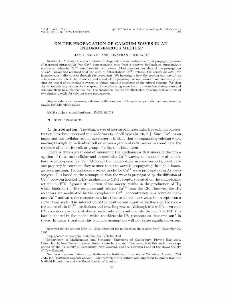
The variable u is usually taken as denoting the concentration of the species (U say)that is propagating the wave. This simple model (the piecewise linear Fitzhugh–Nagumo model) has been widely studied and it is well known that it has a travelingwave solution of the form shown in Fig. 1 [19]. Note that the reaction term, f(u), has

CALCIUM WAVES IN INHOMOGENEOUS MEDIUM 75

x

u

u = 1

speed = c

FIG. 1. Schematic diagram of the form of the traveling wave in the piecewise linear Fitzhugh–Nagumo equation.

a discontinuity at x = α; if u > α the reaction term will drive u toward 1, while ifu < α the reaction term will drive u to 0. Thus, α acts as a threshold. Throughoutmost of this paper we shall scale the space variable, x, by

√D so that D no longer

appears explicitly.In this model, excitability arises due to the properties of the reaction term, f , and

it is generally assumed that f is given by (2) along the entire x-axis. This is equivalentto assuming that the reaction terms that lead to the release of U are homogeneouslydistributed. However, in many biological situations this may not be the case. Regionswhere f is given by (2) (active regions) may be separated by regions where there isno release of U or the kinetics are different (passive regions, or gaps).

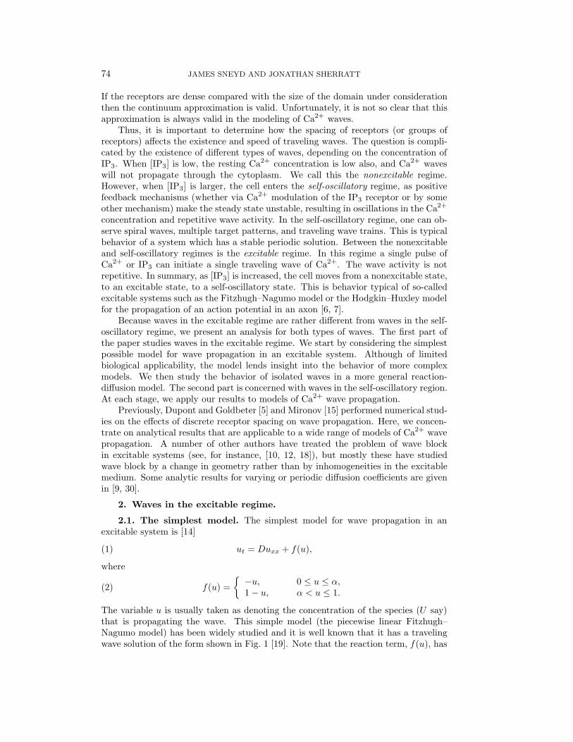
2.2. Wave propagation across a gap. To investigate how a wave will prop-agate across a passive region, we set f = 0 on the interval [L,L + w], as shown inFig. 2. This interval where the wave is not being actively propagated shall be calledthe gap. The x-axis is thus divided into three regions: region I, (−∞, L); region II,[L,L+ w]; and region III, (L+ w,∞).

A traveling wave propagating along the x-axis from left to right will cross thegap (and continue to +∞) if and only if, at steady state, u(L + w) > α (cf. Fig.2). This is because α is the point of discontinuity (i.e., the threshold) of the reactionterm. As soon as u gets above α at the right edge of the gap, f(u) will be positivethere, initiating an autocatalytic release of u that will initiate wave propagation onthe right-hand side of the gap.

Let uI , uII , and uIII denote the solutions to (1) in regions I, II, and III, respec-tively. The steady state equations are

u′′I = −(1− uI),(3)u′′II = 0,(4)u′′III = uIII ,(5)

and thus

uI = Aex + 1,(6)


x

u

Region IIpassive

Region IIIactive

Region Iactive

u'' + f(u) = 0 u'' + f(u) = 0u'' = 0

b

α

L L+w

gap

FIG. 2. Illustration of active and passive regions. An active region is where the reaction term,f(u), is nonzero, while a passive region is where f = 0. Thus, u can move across the gap by passivediffusion only.

uII = Cx+D,(7)uIII = Ee−x,(8)

where we have used boundedness at ±∞ and where A, C, D, and E are constantsto be determined. Constraining the steady state solution to be continuous with acontinuous derivative at L and L+ w gives the constraint equations

AeL + 1 = CL+D,(9)C(L+ w) +D = Ee−(L+w),(10)

AeL = C,(11)C = −Ee−(L+w).(12)

Recalling that u(L + w) = α defines the critical gap width, we can then solve for wto get

w =1α− 2.(13)

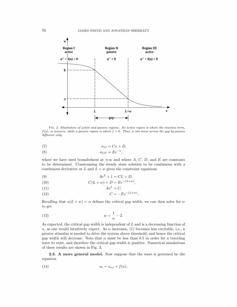
As expected, the critical gap width is independent of L and is a decreasing function ofα, as one would intuitively expect. As α increases, (1) becomes less excitable, i.e., agreater stimulus is needed to drive the system above threshold, and hence the criticalgap width will decrease. Note that α must be less than 0.5 in order for a travelingwave to exist, and therefore the critical gap width is positive. Numerical simulationsof these results are shown in Fig. 3.

2.3. A more general model. Now suppose that the wave is governed by theequation

ut = uxx + f(u),(14)


1.0

0.8

0.6

0.4

0.2

0.0

u

252015105x

gap width = 2.85

1.0

0.8

0.6

0.4

0.2

0.0

u

252015105x

gap width = 3.1 B

A

FIG. 3. Numerical solutions to (1), with α = 0.2. The critical width is thus 3. (A) When thegap is small enough the wave slows down at the gap, but eventually crosses it. (B) When the gap iswider than the critical width, the wave is not able to cross the gap. The steady solution in the gapis then just a straight line connecting the solutions on either side of the gap.

where f(u) takes the general nonlinear form shown in Fig. 4(A). Equation (14) hastwo stable steady states at u = 0 and u = u1, and, as before, the saddle point atu = α acts as a threshold.

Set up the domain as before, with a gap (i.e., f = 0) on the interval [L,L + w]and active kinetics on (−∞, L) and (L+w,∞). At steady state u′′ = −f(u) and thus

12d

dx(u′)2 =

d

dxG(u),(15)

where

G(u) = −∫ u

u0

f(v) dv.(16)


-0.005

-0.004

-0.003

-0.002

-0.001

0.000

G(u

)

0.70.60.50.40.30.20.10.0 u

0.02

0.01

0.00

-0.01

h

0.50.40.30.20.10.0u

u = α u = u1

A

B

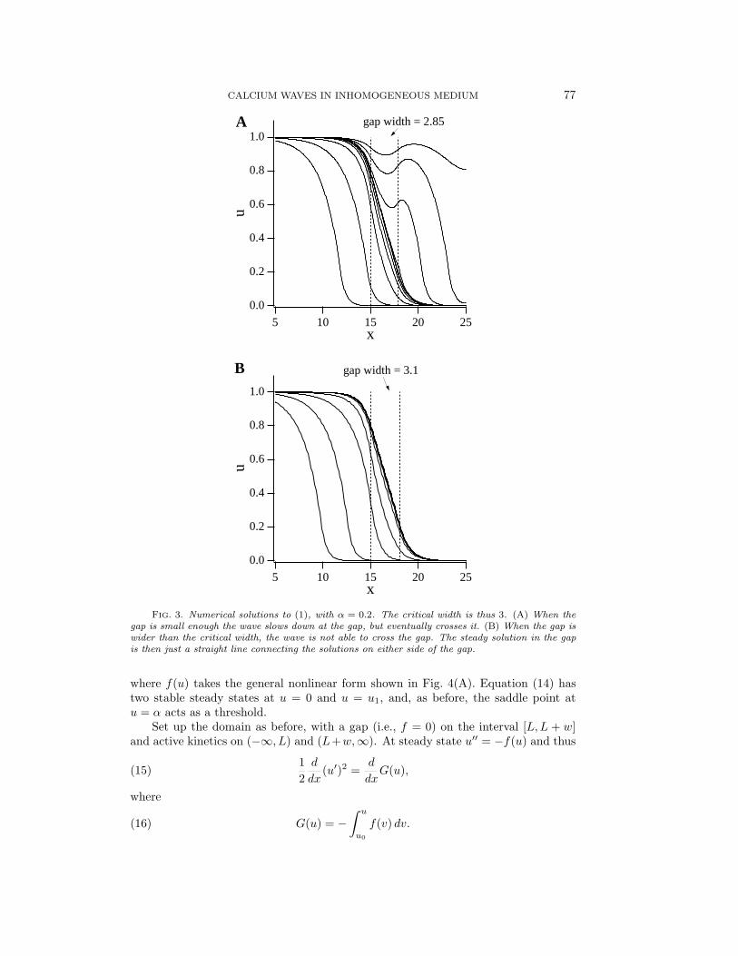
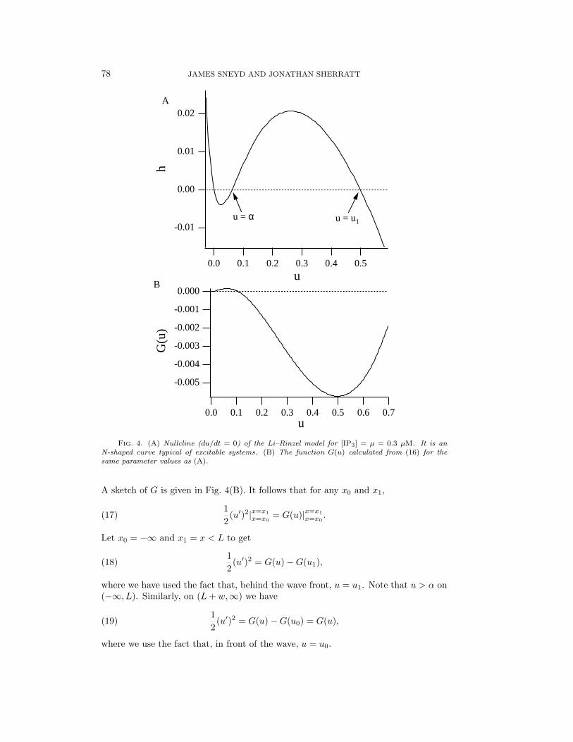
FIG. 4. (A) Nullcline (du/dt = 0) of the Li–Rinzel model for [IP3] = µ = 0.3 µM. It is anN-shaped curve typical of excitable systems. (B) The function G(u) calculated from (16) for thesame parameter values as (A).

A sketch of G is given in Fig. 4(B). It follows that for any x0 and x1,

12

(u′)2|x=x1x=x0

= G(u)|x=x1x=x0

.(17)

Let x0 = −∞ and x1 = x < L to get

12

(u′)2 = G(u)−G(u1),(18)

where we have used the fact that, behind the wave front, u = u1. Note that u > α on(−∞, L). Similarly, on (L+ w,∞) we have

12

(u′)2 = G(u)−G(u0) = G(u),(19)

where we use the fact that, in front of the wave, u = u0.


On the interval [L,L + w], a steady state solution for u must be a straight line,and thus matching the slopes of u at L and L+ w gives

12

(u(L)− u(L+ w)

w

)2

= G[u(L)]−G(u1) = G[u(L+ w)] .(20)

This equation has a solution for values of u(L+ w) either side of the threshold valueα. However, we expect intuitively that the steady state can only be stable whenu(L + w) < α, and this is confirmed by numerical simulation. Thus the critical gapwidth above which the wave cannot propagate is given by u(L+w) = α; substitutingthis into (20) and eliminating u(L) gives an equation for w with a unique solution.

2.3.1. Inclusion of degradation in the gap. In many situations the wavevariable, u, does not simply diffuse across the gap but is degraded or removed aswell. For instance, the regions of active kinetics could refer to regions where there aremany IP3 receptors, but in between these regions Ca2+ does not simply diffuse but ispumped back into the ER. Therefore, a more realistic model could include the effectof the removal of u in the gap.

We make the simplest assumption that the removal of u in the gap is a first-orderprocess, i.e.,

ut = uxx − δ2u,(21)

and, thus, in the gap

u′′ = δ2u(22)

at steady state for some constant δ. A similar analysis to the above shows that thecritical gap width, w, and u(L) are given by

α− u(L) cosh(δw) = −1δ

sinh(δw)√

2[G[u(L)]−G(u1)],(23)

α cosh(δw)− u(L) = −1δ

sinh(δw)√

2G(α).(24)

2.4. Application to calcium waves. Li and Rinzel [13] have proposed a modelfor Ca2+ oscillations based on a reduction of a previous model by DeYoung andKeizer [4]. The model includes terms that describe the Ca2+ current through the IP3receptor, modulation of the receptor current by IP3 and Ca2+, leak of Ca2+ out ofthe ER, and reuptake of Ca2+ by an ATPase pump. The model equations take theform

du

dt= f(u, h;µ),(25)

τh(u;µ)dh

dt= h∞(u;µ)− h,(26)

where u denotes [Ca2+] and µ, which denotes [IP3], is treated as a bifurcation param-eter. The complete model equations, and the parameters we used for computations,are given in the appendix. The nullcline f(u, h;µ = 0.3) = 0 is graphed in Fig. 4(A),where for simplicity the steady state has been shifted to the origin. It is an N-shapedcurve typical of models of excitable systems. Assuming h to be a slow variable andincorporation of Ca2+ diffusion in one space dimension give

ut = Dcuxx + f(u, h0;µ),(27)


350

300

250

200

150

100

50

crit

ical

gap

wid

th (

µm)

0.320.310.300.290.280.27

[IP3] (µM)

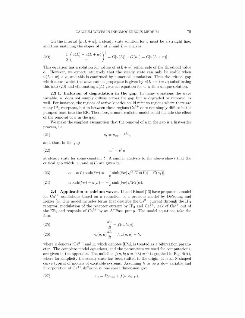
FIG. 5. Critical gap width as a function of [IP3] for the Li–Rinzel model [13]. As [IP3] increases,the critical width becomes large since the threshold, α, is decreasing to zero, but the time taken forthe wave to cross the gap also tends to infinity (computations not shown).

where Dc is the diffusion coefficient of Ca2+ and h0 is the steady state of h. Note thatsince h is a slow variable, h is constant over the wave front. We implicitly assume thatCa2+ buffers may be approximated by an apparent diffusion coefficient, an assumptionwhich has many dangers [26, 29], but a full discussion of the complications caused bybuffers is outside the scope of this paper. G(u), defined by (16), is plotted in Fig. 4(B).In Fig. 5 we plot the critical width as a function of µ. We used Dc = 25 µm2s−1,a value obtained experimentally in Xenopus cytoplasm [1]. In general, since thediffusion coefficient merely sets the length scale, it is sufficient to calculate the criticalwidth for the case Dc = 1 and then rescale appropriately. The critical width hasa very sensitive dependence on [IP3] and is less than 20 µm for low IP3. This isconsistent with the results of Parker and Yao [17], who observed punctate release ofCa2+ from isolated “hot spots” in Xenopus at concentrations of IP3 that were too lowto initiate propagating waves. Nevertheless, the quantitative model predictions shouldbe treated with caution, as the calculation of the critical width does not take receptorinactivation into account. Relaxing the assumption that h is a slow variable will givemore accurate predictions, but as yet we have not been able to do this analytically.

3. Waves in the self-oscillatory regime. Consider the reaction-diffusion sys-tem

ut = uxx +M(x)f(u, v),(28)vt = M(x)g(u, v).(29)

We assume the medium is inhomogeneous and thus the reaction terms f and g aremodulated by M(x). In order to make the problem tractable, we shall assume thatM is periodic and piecewise constant and divides the spatial domain into alternatingactive and passive regions (Fig. 6). Each active region is of width L1, and each


L1 L2

activeregion

passiveregion

M(x)

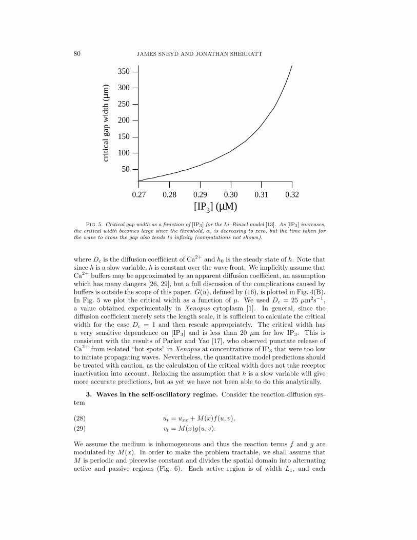
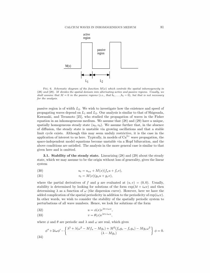
FIG. 6. Schematic diagram of the function M(x) which controls the spatial inhomogeneity in(28) and (29). M divides the spatial domain into alternating active and passive regions. Usually, weshall assume that M = 0 in the passive regions (i.e., that b1, . . . , b4 = 0), but that is not necessaryfor the analysis.

passive region is of width L2. We wish to investigate how the existence and speed ofpropagating waves depend on L1 and L2. Our analysis is similar to that of Shigesada,Kawasaki, and Teramoto [25], who studied the propagation of waves in the Fisherequation in an inhomogeneous medium. We assume that (28) and (29) have a unique,spatially homogeneous steady state (u0, v0). We assume further that, in the absenceof diffusion, the steady state is unstable via growing oscillations and that a stablelimit cycle exists. Although this may seem unduly restrictive, it is the case in theapplication of interest to us here. Typically, in models of Ca2+ wave propagation, thespace-independent model equations become unstable via a Hopf bifurcation, and theabove conditions are satisfied. The analysis in the more general case is similar to thatgiven here and is omitted.

3.1. Stability of the steady state. Linearizing (28) and (29) about the steadystate, which we may assume to be the origin without loss of generality, gives the linearsystem

ut = uxx +M(x)(fuu+ fvv),(30)vt = M(x)(guu+ gvv),(31)

where the partial derivatives of f and g are evaluated at (u, v) = (0, 0). Usually,stability is determined by looking for solutions of the form exp(λt + iωx) and thendetermining λ as a function of ω (the dispersion curve). However, here we have theadded complication of the spatial periodicity in addition to the periodicity of exp(iωx).In other words, we wish to consider the stability of the spatially periodic system toperturbations of all wave numbers. Hence, we look for solutions of the form

u = φ(x)eλt+iωx,(32)v = θ(x)eλt+iωx,(33)

where φ and θ are periodic and λ and ω are real, which gives

φ′′+2iωφ′−{λ2 + λ(ω2 −Mfu −Mgv) +M2(fugv − fvgu)−Mgvω

2

(λ−Mgv)

}φ = 0.

(34)


Let

M(x)(fu fvgu gv

)=

(a1 a2a3 a4

), active region,(

b1 b2b3 b4

), passive region,

(35)

where a1, . . . , a4 and b1, . . . , b4 are constants. Then, the condition for the existenceof a C1 periodic solution of (34) is

α2 + β2

2αβsinh(αL1) sinh(βL2) + cosh(αL1) cosh(βL2) = cos[ω(L1 + L2)],(36)

where

α =

√λ2 − λ(a1 + a4) + (a1a4 − a2a3)

(λ− a4),(37)

β =

√λ2 − λ(b1 + b4) + (b1b4 − b2b3)

(λ− b4).(38)

For a fixed L1 and L2, (36) defines λ as a function of ω. The maximum ofλ(ω) defines the fastest growing mode; if λ > 0 at this maximum, the steady stateis unstable, while if λ < 0 at the maximum, the steady state is stable. Thus, inprinciple it is possible to calculate the boundary between stability and instability fora particular model. In the application to Ca2+ waves we are most interested in thecase when L1 and L2 are small, as in general they are both considerably smaller thanthe diffusion coefficient of Ca2+. So, let L1 = εL̃1, L2 = εL̃2, where ε� 1. Then, toleading order in ε, (36) becomes

12

(α2 + β2)L̃1L̃2 +12α2L̃2

1 +12β2L̃2

2 = −ω2

2(L̃1 + L̃2)2(39)

and thus

α2L̃1 + β2L̃2 = −ω2(L̃1 + L̃2).(40)

Substituting in the expressions for α and β and assuming for convenience that b1, . . . , b4are zero give

(L̃1+L̃2)λ2−{(a1+a4)L̃1+a4L̃2−ω2(L̃1+L̃2)}λ+L̃1(a1a4−a2a3)−ω2a4(L̃1+L̃2) = 0.(41)In order for the solutions to this equation to have negative real part for all ω, we musthave that

L̃1(a1 + a4) + a4L̃2 < 0(42)

and thus

L̃1 <−a4

a1 + a4L̃2.(43)

Since a1 + a4 > 0 (because by assumption the homogeneous steady state is unstablevia growing oscillations), this requires a4 < 0, which is the case for the models ofCa2+ waves we discuss here.

When L2 = 0, (36) reduces to

λ2 + λ(ω2 − a1 − a4) + a1a4 − a2a3 − a4ω2 = 0,(44)

which is the usual dispersion equation for a homogeneous domain.


3.0

2.5

2.0

1.5

1.0

0.5

0.0

L2

(µm

)

1086420 L1 (µm)

µ = 0.6

µ = 0.65

µ = 0.55

Unstable region

Stable region

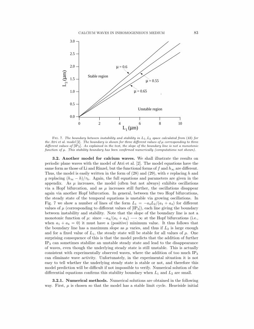
FIG. 7. The boundary between instability and stability in L1, L2 space calculated from (43) forthe Atri et al. model [2]. The boundary is shown for three different values of µ corresponding to threedifferent values of [IP3]. As explained in the text, the slope of the boundary line is not a monotonicfunction of µ. This stability boundary has been confirmed numerically (computations not shown).

3.2. Another model for calcium waves. We shall illustrate the results onperiodic plane waves with the model of Atri et al. [2]. The model equations have thesame form as those of Li and Rinzel, but the functional forms of f and h∞ are different.Thus, the model is easily written in the form of (28) and (29), with v replacing h andg replacing (h∞ − h)/τh. Again, the full equations and parameters are given in theappendix. As µ increases, the model (often but not always) exhibits oscillationsvia a Hopf bifurcation, and as µ increases still further, the oscillations disappearagain via another Hopf bifurcation. In general, between the two Hopf bifurcations,the steady state of the temporal equations is unstable via growing oscillations. InFig. 7 we show a number of lines of the form L1 = −a4L2/(a1 + a4) for differentvalues of µ (corresponding to different values of [IP3]), each line giving the boundarybetween instability and stability. Note that the slope of the boundary line is not amonotonic function of µ: since −a4/(a1 + a4) −→ ∞ at the Hopf bifurcations (i.e.,when a1 + a4 = 0) it must have a (positive) minimum value. It thus follows thatthe boundary line has a maximum slope as µ varies, and thus if L2 is large enoughand for a fixed value of L1, the steady state will be stable for all values of µ. Onesurprising consequence of this is that the model predicts that the addition of furtherIP3 can sometimes stabilize an unstable steady state and lead to the disappearanceof waves, even though the underlying steady state is still unstable. This is actuallyconsistent with experimentally observed waves, where the addition of too much IP3can eliminate wave activity. Unfortunately, in the experimental situation it is noteasy to tell whether the underlying steady state is stable or not, and therefore thismodel prediction will be difficult if not impossible to verify. Numerical solution of thedifferential equations confirms this stability boundary when L1 and L2 are small.

3.2.1. Numerical methods. Numerical solutions are obtained in the followingway. First, µ is chosen so that the model has a stable limit cycle. Heaviside initial


conditions are used for c. Thus, at t = 0, c on the left portion of the domain (usuallythe 10 leftmost spatial grid points) is raised above steady state, initiating oscillationsin the leftmost region of the domain. If stable periodic waves exist, these oscillationsgradually invade the entire domain. However, if the periodic wave is unstable, theoscillations gradually disappear. By looking at the existence of periodic waves fordifferent (small) values of L1 and L2, we were able to confirm the predicted stabilityboundary. The differential equations were solved using an implicit time-steppingscheme and central space differences.

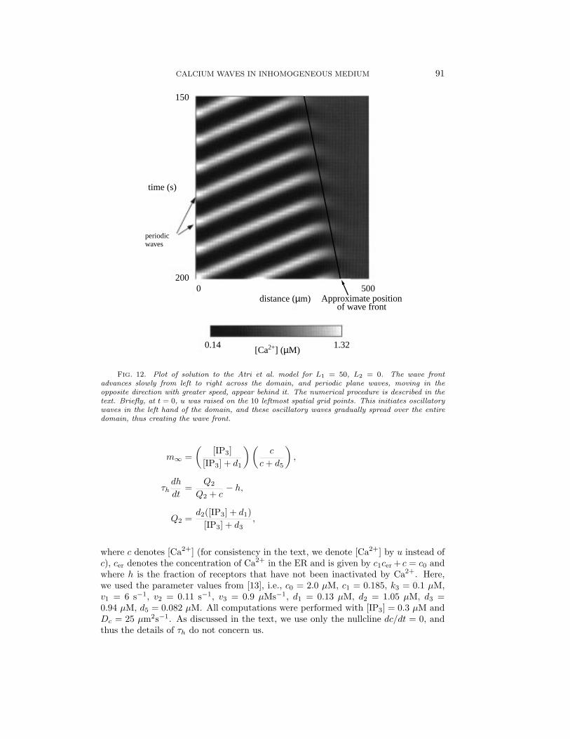
3.2.2. Periodic waves and the wave front. It is crucial to note that, in thenumerical solutions, two very different types of waves appear. We distinguish themby the terms periodic wave and wave front. This is most easily illustrated by referenceto Fig. 12, which shows the situation a short time after t = 0 for the case L2 = 0 andwhen Heaviside initial conditions for c were used, as described above. Periodic wavesexist for this value of L2 because the domain is homogeneous with oscillatory kinetics.The periodic wave can be clearly seen as a series of white bands sloping up from leftto right. These correspond to a periodic wave moving from right to left across thedomain. However, the periodic wave is not the same as the wave front. As timeincreases, each successive peak of the periodic wave is initiated from a region that ismoving slowly from left to right. This we call the wave front of the periodic wave;its approximate position is marked by a line in Fig. 12. When t is large enough, thewave front will have moved across the entire domain, leaving only the periodic wavein its wake. Note that the wave front is moving from left to right with a speed thatis much less than that of the periodic wave which is moving in the opposite direction.The analysis in the present paper is confined to studying the speed of the wave front,not the speed of the subsequent periodic wave. It is also important to note that thewave front, which we define as the place where c = 0.05 µM, does not move acrossthe domain monotonically (cf. Fig. 10). This is caused by the oscillatory nature ofthe kinetics. Nevertheless, the average wave front speed may still be defined as theslope of the best fit line through the wave front.

Extensive numerical simulations with different initial conditions and values of µshow that the periodic wave can travel with a wide range of speeds in either direction.In some cases, as in Fig. 12, it starts at the wave front, travels backward across thedomain, and is absorbed by the left-hand boundary. In other cases, the periodic waveis initiated at the left-hand boundary and travels from left to right until it hits thewave front and disappears. Sherratt [22, 24, 23] discusses this in detail for periodicwaves in λ− ω systems. A useful interpretation of the wave front speed is the speedat which a periodic wave can “invade” a domain. However, the actual speed anddirection of the periodic wave can be very different from the speed at which thatperiodic wave invades a domain.

3.3. The dispersion curve. The oscillatory nature of the kinetics means thatwave solutions of (28) and (29) are not simple transition waves, as in the excitablecase. Rather, they have the form of a moving wave front with spatiotemporal os-cillations behind the front (as described above). We focus on the movement of theleading wave front, which we study using the linearized equations (30) and (31). Thelinear analysis will apply to the front of the nonlinear wave and will provide an ap-proximate estimate for the nonlinear wave front speed. Numerical results confirmthe approximate accuracy of estimates from the linear theory. We first consider thespatially homogeneous case and use this as a guide to the analysis of the spatiallyheterogeneous case.


We emphasize that in both the homogeneous and the heterogeneous cases, ouranalysis is a local one only and therefore applies only to the movement of the wavefront. The speed of the periodic waves behind the wave front cannot be treated byour methods. In fact, we have as yet been unable to determine the speed of theperiodic waves as a function of L1 and L2. This requires a nonlinear analysis whichis considerably more difficult than that presented here.

3.3.1. Spatially homogeneous case. It is helpful to consider first the slightlydifferent case where u and v have equal diffusion coefficients, i.e.,

ut = uxx + fuu+ fvv,(45)vt = vxx + guu+ gvv.(46)

By a change of coordinates these equations can be written in the form

ut = uxx + αu+ ωv,(47)vt = vxx − ωu+ αv.(48)

Define new coordinates by u = r cos θ, v = r sin θ and convert to r, θ coordinates toget

rt = rxx − rθ2x + αr,(49)

θt = θxx + 2rxθxr− ω.(50)

Linearizing about the wave front, where r = θx = 0 [23], gives

rt = rxx + αr.(51)

Since (51) is the same form as the linearization of Fisher’s equation, we merely applyprevious results (see, for example, [8, 11, 16]) to determine the wave front speed. Letz = x − ct, where c is the wave front speed. Then, looking for solutions of the formr = exp(−sz) gives cs = s2 + α and thus c = s + α/s. In general, the wave speeddepends on the initial conditions. However, for Heaviside initial conditions of the typeused here the wave travels with the minimum speed. Since this type of initial conditionis the only one used experimentally and is thus the only case of physiological interest,we do not consider any other initial conditions. Thus the observed wave speed, co, isgiven by co = 2

√α.

Unfortunately, this change of variables does not work if v and u have differentdiffusion coefficients. Previous work on λ−ω systems [22, 24, 23] shows that in frontof the wave θ does not go to zero but increases (i.e., oscillates) according to θ = ωt. Itis reasonable to expect that something similar happens here also. This suggests thatthe wave front is not only oscillatory in z but also oscillatory in t, which motivatesthe following analysis. Let D be the diffusion coefficient of v, i.e.,

ut = uxx + αu+ ωv,(52)vt = Dvxx − ωu+ αv,(53)

and look for solutions of the form u = Ae−szeiωt v = Be−szeiωt for some real constantsA and B and where s is complex. The solvability condition for A and B turns out tobe

(ξ − σ1)(ξ − σ2) = −ω2,(54)


where ξ = cs, σ1 = Ds2 + α− iω, and σ2 = s2 + α− iω. Letting s = γ + iδ gives

φ1(c, δ) = 0,(55)φ2(c, δ) = 0,(56)

where

φ1(c, δ) = (cγ −Dγ2 +Dδ2 − α)(cγ − γ2 + δ2 − α)− (cδ − 2Dγδ + ω)(cδ − 2γδ + ω) + ω2,(57)

φ2(c, δ) = (cγ −Dγ2 +Dδ2 − α)(cδ − 2γδ + ω)+ (cγ − γ2 + δ2 − α)(cδ − 2Dγδ + ω).(58)

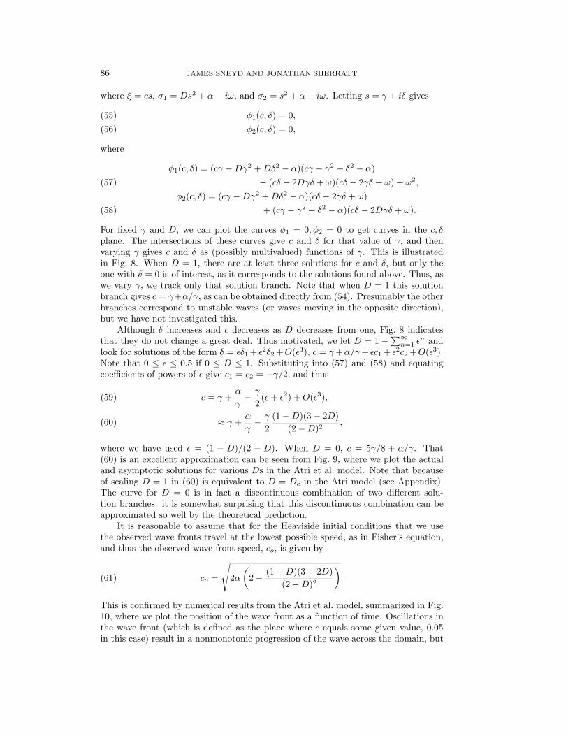
For fixed γ and D, we can plot the curves φ1 = 0, φ2 = 0 to get curves in the c, δplane. The intersections of these curves give c and δ for that value of γ, and thenvarying γ gives c and δ as (possibly multivalued) functions of γ. This is illustratedin Fig. 8. When D = 1, there are at least three solutions for c and δ, but only theone with δ = 0 is of interest, as it corresponds to the solutions found above. Thus, aswe vary γ, we track only that solution branch. Note that when D = 1 this solutionbranch gives c = γ+α/γ, as can be obtained directly from (54). Presumably the otherbranches correspond to unstable waves (or waves moving in the opposite direction),but we have not investigated this.

Although δ increases and c decreases as D decreases from one, Fig. 8 indicatesthat they do not change a great deal. Thus motivated, we let D = 1−

∑∞n=1 ε

n andlook for solutions of the form δ = εδ1 + ε2δ2 +O(ε3), c = γ+α/γ+ εc1 + ε2c2 +O(ε3).Note that 0 ≤ ε ≤ 0.5 if 0 ≤ D ≤ 1. Substituting into (57) and (58) and equatingcoefficients of powers of ε give c1 = c2 = −γ/2, and thus

c = γ +α

γ− γ

2(ε+ ε2) +O(ε3),(59)

≈ γ +α

γ− γ

2(1−D)(3− 2D)

(2−D)2 ,(60)

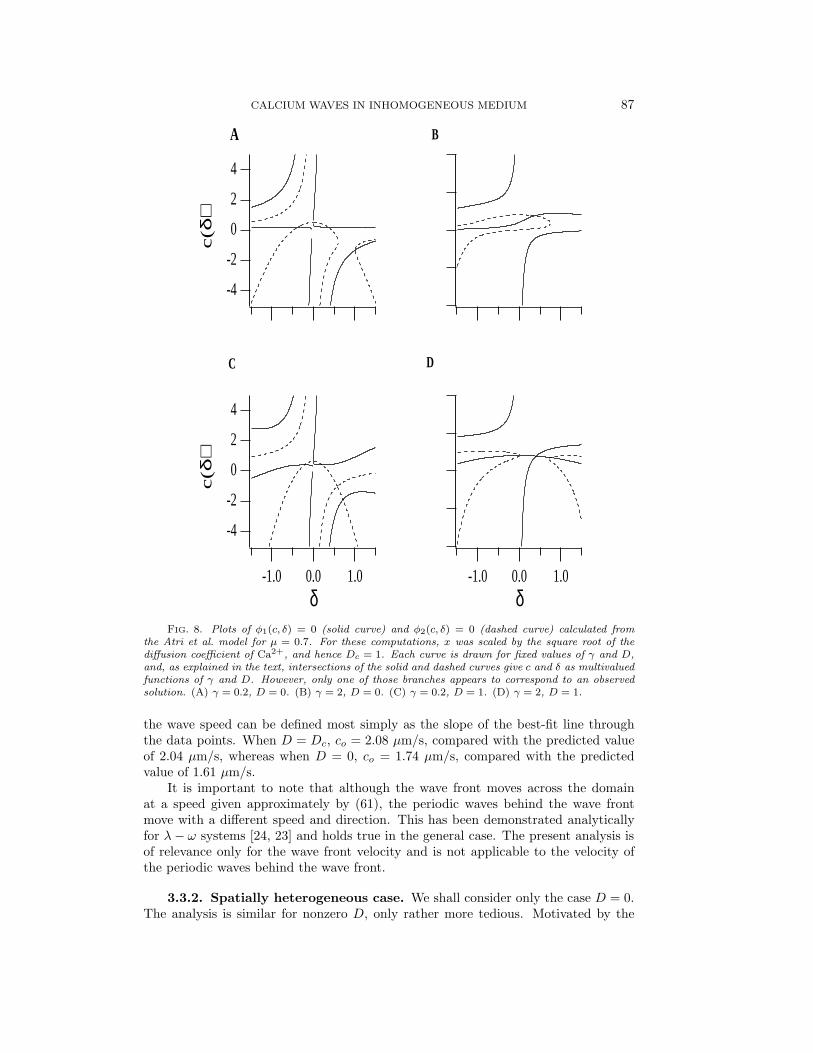
where we have used ε = (1 − D)/(2 − D). When D = 0, c = 5γ/8 + α/γ. That(60) is an excellent approximation can be seen from Fig. 9, where we plot the actualand asymptotic solutions for various Ds in the Atri et al. model. Note that becauseof scaling D = 1 in (60) is equivalent to D = Dc in the Atri model (see Appendix).The curve for D = 0 is in fact a discontinuous combination of two different solu-tion branches: it is somewhat surprising that this discontinuous combination can beapproximated so well by the theoretical prediction.

It is reasonable to assume that for the Heaviside initial conditions that we usethe observed wave fronts travel at the lowest possible speed, as in Fisher’s equation,and thus the observed wave front speed, co, is given by

co =

√2α(

2− (1−D)(3− 2D)(2−D)2

).(61)

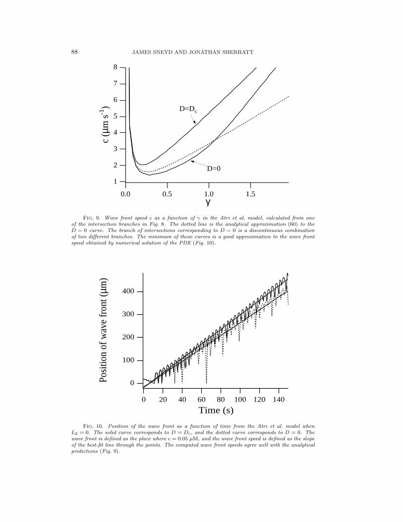
This is confirmed by numerical results from the Atri et al. model, summarized in Fig.10, where we plot the position of the wave front as a function of time. Oscillations inthe wave front (which is defined as the place where c equals some given value, 0.05in this case) result in a nonmonotonic progression of the wave across the domain, but


-4

-2

0

2

4

c(δ

)

1.00.0-1.0δ

-4

-2

0

2

4

c(δ

)

1.00.0-1.0δ

A B

C D

FIG. 8. Plots of φ1(c, δ) = 0 (solid curve) and φ2(c, δ) = 0 (dashed curve) calculated fromthe Atri et al. model for µ = 0.7. For these computations, x was scaled by the square root of thediffusion coefficient of Ca2+, and hence Dc = 1. Each curve is drawn for fixed values of γ and D,and, as explained in the text, intersections of the solid and dashed curves give c and δ as multivaluedfunctions of γ and D. However, only one of those branches appears to correspond to an observedsolution. (A) γ = 0.2, D = 0. (B) γ = 2, D = 0. (C) γ = 0.2, D = 1. (D) γ = 2, D = 1.

the wave speed can be defined most simply as the slope of the best-fit line throughthe data points. When D = Dc, co = 2.08 µm/s, compared with the predicted valueof 2.04 µm/s, whereas when D = 0, co = 1.74 µm/s, compared with the predictedvalue of 1.61 µm/s.

It is important to note that although the wave front moves across the domainat a speed given approximately by (61), the periodic waves behind the wave frontmove with a different speed and direction. This has been demonstrated analyticallyfor λ− ω systems [24, 23] and holds true in the general case. The present analysis isof relevance only for the wave front velocity and is not applicable to the velocity ofthe periodic waves behind the wave front.

3.3.2. Spatially heterogeneous case. We shall consider only the case D = 0.The analysis is similar for nonzero D, only rather more tedious. Motivated by the


8

7

6

5

4

3

2

1

c (µ

m s

-1)

1.51.00.50.0γ

D=0

D=Dc

FIG. 9. Wave front speed c as a function of γ in the Atri et al. model, calculated from oneof the intersection branches in Fig. 8. The dotted line is the analytical approximation (60) to theD = 0 curve. The branch of intersections corresponding to D = 0 is a discontinuous combinationof two different branches. The minimum of these curves is a good approximation to the wave frontspeed obtained by numerical solution of the PDE (Fig. 10).

400

300

200

100

0Posi

tion

of w

ave

fron

t (µm

)

140120100806040200

Time (s)

FIG. 10. Position of the wave front as a function of time from the Atri et al. model whenL2 = 0. The solid curve corresponds to D = Dc, and the dotted curve corresponds to D = 0. Thewave front is defined as the place where c = 0.05 µM, and the wave front speed is defined as the slopeof the best-fit line through the points. The computed wave front speeds agree well with the analyticalpredictions (Fig. 9).


analysis of Shigesada, Kawasaki, and Teramoto [25] and the form of the solution inthe spatially homogeneous case, we look for solutions of the form u = U(z)φ(x)eiωt,v = V (z)θ(x)eiωt, where φ and θ are periodic and U, V −→ 0 as z −→∞. The reasonfor looking for solutions of such a form is not immediately clear. We argue that it isreasonable to expect the wave front to consist of three parts; first, a profile dependenton z that determines the overall wave shape (U and V ); second, a spatially periodicvariation caused by the underlying periodicity of the medium (φ and θ); and third,a temporal periodicity caused by the oscillatory nature of the kinetics (eiωt). Weemphasize that such a solution will apply only to the wave front, not necessarily tothe (nonlinear) periodic waves that occur behind the wave front. Substituting into(30) and (31) gives(

−cU′

U+ iω

)φ =

(U ′′

Uφ+

2U ′

Uφ′ + φ′′

)+Mfuφ+M

V

Ufvθ,(62) (

−cV′

V+ iω

)θ = M

U

Vguφ+Mgvθ.(63)

It follows that U ′/U , U ′′/U , and U/V must all be constant, and hence

U = Ae−sz,(64)V = BU(65)

for some constants A, B, and s, where s is complex. Solving for φ now gives

φ′′ − 2sφ′ +(s2 − (cs+ iω) +Mfu +

M2fvgu(cs+ iω)−Mgv

)φ = 0.(66)

The condition for the existence of a periodic solution to (66) is

cosh(s(L1 + L2)) = cosh(q1L1) cosh(q2L2) +q21 + q2

2

2q1q2sinh(q1L1) sinh(q2L2),(67)

where

q1 =

√(cs+ iω)2 − 2(cs+ iω)α+ α2 + ω2

(cs+ iω − α),(68)

q2 =√cs+ iω.(69)

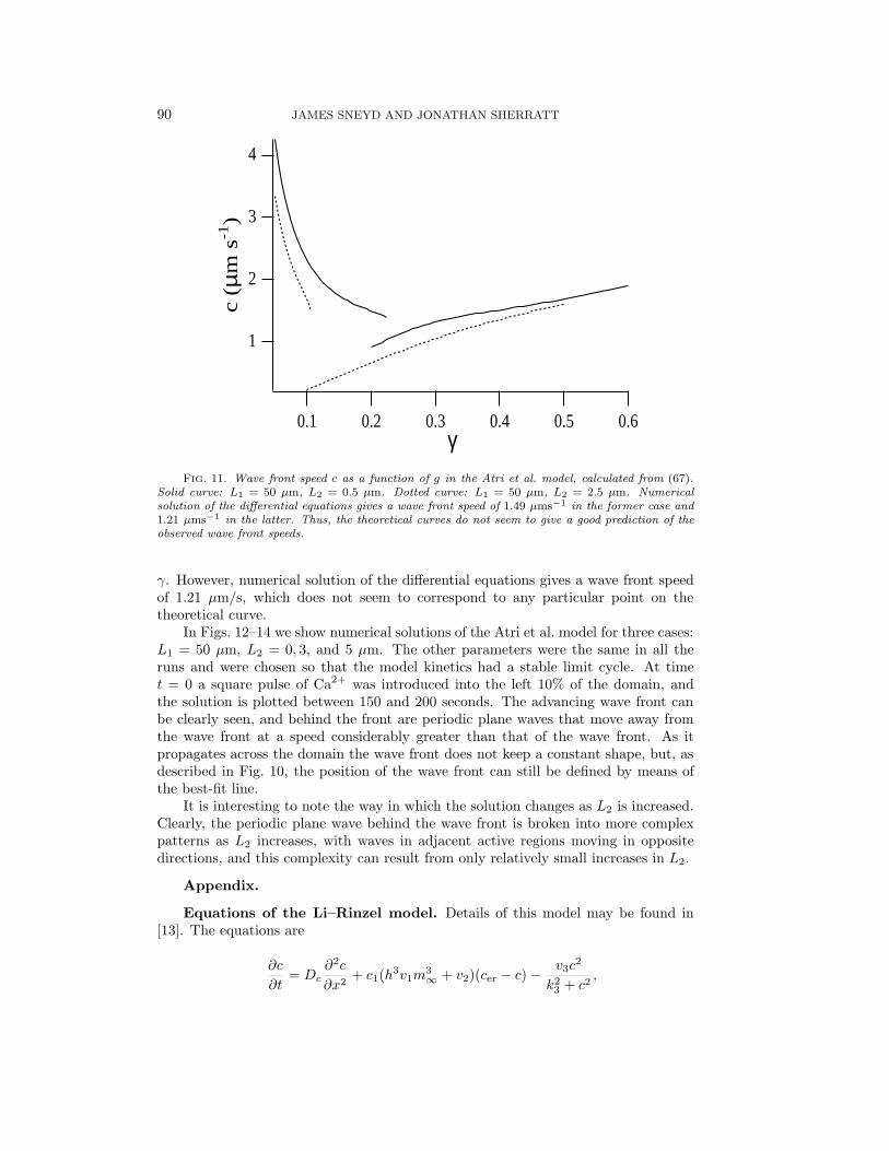
This is the same equation given by Shigesada, Kawasaki, and Teramoto but withdifferent definitions for q1 and q2. We have implicitly assumed that b1, . . . , b4 =0 and that in the active region (30) and (31) are written in the form of (52) and(53). When L2 = 0, c can be determined as a function of γ from (67), giving thesame curve as in Fig. 9 (the D = 0 curve). We mentioned then that this curve isactually a discontinuous combination of two different branches. As L2 is increased,this discontinuity becomes more pronounced, as can be seen from Fig. 11, which showscurves of c versus γ for two different values of L2. The solid curve corresponds toL1 = 50 µm, L2 = 0.5 µm, while the dotted curve corresponds to the same value forL1 but with L2 = 2.5 µm. This makes it difficult to predict the exact wave frontspeed merely from consideration of the roots of (67). For instance, when L1 = 50and L2 = 2.5, the dotted curve in Fig. 11 gives the theoretical prediction of c vs.


4

3

2

1

c (µ

m s

-1)

0.60.50.40.30.20.1γ

FIG. 11. Wave front speed c as a function of g in the Atri et al. model, calculated from (67).Solid curve: L1 = 50 µm, L2 = 0.5 µm. Dotted curve: L1 = 50 µm, L2 = 2.5 µm. Numericalsolution of the differential equations gives a wave front speed of 1.49 µms−1 in the former case and1.21 µms−1 in the latter. Thus, the theoretical curves do not seem to give a good prediction of theobserved wave front speeds.

γ. However, numerical solution of the differential equations gives a wave front speedof 1.21 µm/s, which does not seem to correspond to any particular point on thetheoretical curve.

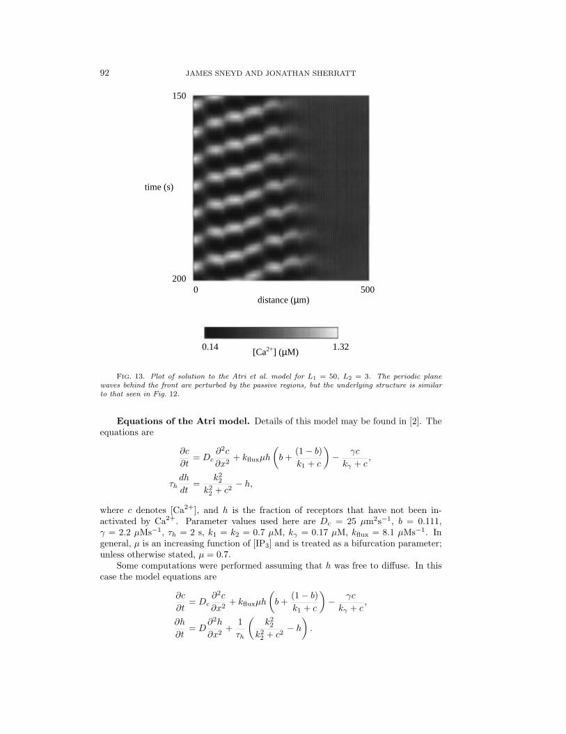
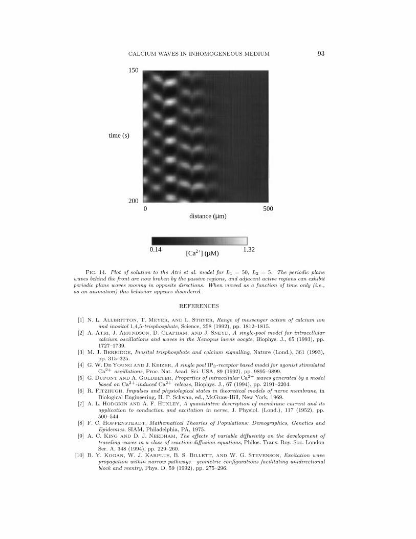
In Figs. 12–14 we show numerical solutions of the Atri et al. model for three cases:L1 = 50 µm, L2 = 0, 3, and 5 µm. The other parameters were the same in all theruns and were chosen so that the model kinetics had a stable limit cycle. At timet = 0 a square pulse of Ca2+ was introduced into the left 10% of the domain, andthe solution is plotted between 150 and 200 seconds. The advancing wave front canbe clearly seen, and behind the front are periodic plane waves that move away fromthe wave front at a speed considerably greater than that of the wave front. As itpropagates across the domain the wave front does not keep a constant shape, but, asdescribed in Fig. 10, the position of the wave front can still be defined by means ofthe best-fit line.

It is interesting to note the way in which the solution changes as L2 is increased.Clearly, the periodic plane wave behind the wave front is broken into more complexpatterns as L2 increases, with waves in adjacent active regions moving in oppositedirections, and this complexity can result from only relatively small increases in L2.

Appendix.

Equations of the Li–Rinzel model. Details of this model may be found in[13]. The equations are

∂c

∂t= Dc

∂2c

∂x2 + c1(h3v1m3∞ + v2)(cer − c)−

v3c2

k23 + c2

,


periodic waves

distance (µm)

1.320.14

0

time (s)

200

150

500

[Ca2+] (µM)

Approximate position of wave front

FIG. 12. Plot of solution to the Atri et al. model for L1 = 50, L2 = 0. The wave frontadvances slowly from left to right across the domain, and periodic plane waves, moving in theopposite direction with greater speed, appear behind it. The numerical procedure is described in thetext. Briefly, at t = 0, u was raised on the 10 leftmost spatial grid points. This initiates oscillatorywaves in the left hand of the domain, and these oscillatory waves gradually spread over the entiredomain, thus creating the wave front.

m∞ =(

[IP3][IP3] + d1

)(c

c+ d5

),

τhdh

dt=

Q2

Q2 + c− h,

Q2 =d2([IP3] + d1)

[IP3] + d3,

where c denotes [Ca2+] (for consistency in the text, we denote [Ca2+] by u instead ofc), cer denotes the concentration of Ca2+ in the ER and is given by c1cer + c = c0 andwhere h is the fraction of receptors that have not been inactivated by Ca2+. Here,we used the parameter values from [13], i.e., c0 = 2.0 µM, c1 = 0.185, k3 = 0.1 µM,v1 = 6 s−1, v2 = 0.11 s−1, v3 = 0.9 µMs−1, d1 = 0.13 µM, d2 = 1.05 µM, d3 =0.94 µM, d5 = 0.082 µM. All computations were performed with [IP3] = 0.3 µM andDc = 25 µm2s−1. As discussed in the text, we use only the nullcline dc/dt = 0, andthus the details of τh do not concern us.


distance (µm)

1.320.14

0

time (s)

200

150

500

[Ca2+] (µM)

FIG. 13. Plot of solution to the Atri et al. model for L1 = 50, L2 = 3. The periodic planewaves behind the front are perturbed by the passive regions, but the underlying structure is similarto that seen in Fig. 12.

Equations of the Atri model. Details of this model may be found in [2]. Theequations are

∂c

∂t= Dc

∂2c

∂x2 + kfluxµh

(b+

(1− b)k1 + c

)− γc

kγ + c,

τhdh

dt=

k22

k22 + c2

− h,

where c denotes [Ca2+], and h is the fraction of receptors that have not been in-activated by Ca2+. Parameter values used here are Dc = 25 µm2s−1, b = 0.111,γ = 2.2 µMs−1, τh = 2 s, k1 = k2 = 0.7 µM, kγ = 0.17 µM, kflux = 8.1 µMs−1. Ingeneral, µ is an increasing function of [IP3] and is treated as a bifurcation parameter;unless otherwise stated, µ = 0.7.

Some computations were performed assuming that h was free to diffuse. In thiscase the model equations are

∂c

∂t= Dc

∂2c

∂x2 + kfluxµh

(b+

(1− b)k1 + c

)− γc

kγ + c,

∂h

∂t= D

∂2h

∂x2 +1τh

(k2

2

k22 + c2

− h).


distance (µm)

1.320.14

0

time (s)

200

150

500

[Ca2+] (µM)

FIG. 14. Plot of solution to the Atri et al. model for L1 = 50, L2 = 5. The periodic planewaves behind the front are now broken by the passive regions, and adjacent active regions can exhibitperiodic plane waves moving in opposite directions. When viewed as a function of time only (i.e.,as an animation) this behavior appears disordered.

REFERENCES

[1] N. L. ALLBRITTON, T. MEYER, AND L. STRYER, Range of messenger action of calcium ionand inositol 1,4,5-trisphosphate, Science, 258 (1992), pp. 1812–1815.

[2] A. ATRI, J. AMUNDSON, D. CLAPHAM, AND J. SNEYD, A single-pool model for intracellularcalcium oscillations and waves in the Xenopus laevis oocyte, Biophys. J., 65 (1993), pp.1727–1739.

[3] M. J. BERRIDGE, Inositol trisphosphate and calcium signalling, Nature (Lond.), 361 (1993),pp. 315–325.

[4] G. W. DE YOUNG AND J. KEIZER, A single pool IP3-receptor based model for agonist stimulatedCa2+ oscillations, Proc. Nat. Acad. Sci. USA, 89 (1992), pp. 9895–9899.

[5] G. DUPONT AND A. GOLDBETER, Properties of intracellular Ca2+ waves generated by a modelbased on Ca2+-induced Ca2+ release, Biophys. J., 67 (1994), pp. 2191–2204.

[6] R. FITZHUGH, Impulses and physiological states in theoretical models of nerve membrane, inBiological Engineering, H. P. Schwan, ed., McGraw-Hill, New York, 1969.

[7] A. L. HODGKIN AND A. F. HUXLEY, A quantitative description of membrane current and itsapplication to conduction and excitation in nerve, J. Physiol. (Lond.), 117 (1952), pp.500–544.

[8] F. C. HOPPENSTEADT, Mathematical Theories of Populations: Demographics, Genetics andEpidemics, SIAM, Philadelphia, PA, 1975.

[9] A. C. KING AND D. J. NEEDHAM, The effects of variable diffusivity on the development oftraveling waves in a class of reaction-diffusion equations, Philos. Trans. Roy. Soc. LondonSer. A, 348 (1994), pp. 229–260.

[10] B. Y. KOGAN, W. J. KARPLUS, B. S. BILLETT, AND W. G. STEVENSON, Excitation wavepropagation within narrow pathways—geometric configurations facilitating unidirectionalblock and reentry, Phys. D, 59 (1992), pp. 275–296.


[11] D. A. LARSON, Transient bounds and time-asymptotic behavior of solutions to non-linear equa-tions of Fisher type, SIAM J. Appl. Math., 34 (1978), pp. 93–103.

[12] M. A. LEWIS AND P. GRINDROD, One-way blocks in cardiac tissue: A mechanism for propa-gation failure, Bull. Math. Biol., 53 (1991), pp. 881–899.

[13] Y.-X. LI AND J. RINZEL, Equations for InsP3 receptor-mediated [Ca2+] oscillations derivedfrom a detailed kinetic model: A Hodgkin-Huxley like formalism, J. Theor. Biol., 166(1994), pp. 461–473.

[14] H. P. MCKEAN, Nagumo’s equation, Adv. Math., 4 (1970), pp. 209–223.[15] S. L. MIRONOV, Theoretical analysis of Ca2+ wave propagation along the surface of intracel-

lular stores, J. Theor. Biol., 146 (1990), pp. 87–97.[16] J. D. MURRAY, Mathematical Biology, Springer-Verlag, Berlin, Heidelberg, New York, 1989.[17] I. PARKER AND Y. YAO, Regenerative release of calcium from functionally discrete subcellular

stores by inositol trisphosphate, Proc. Roy. Soc. London Ser. B, 246 (1991), pp. 269–274.[18] J. PAUWELUSSEN, One way traffic of pulses in a neuron, J. Math. Biol., 15 (1982), pp. 151–171.[19] J. RINZEL AND J. B. KELLER, Traveling wave solutions of a nerve conduction equation, Bio-

phys. J., 13 (1973), pp. 1313–1337.[20] T. A. ROONEY AND A. P. THOMAS, Intracellular calcium waves generated by Ins (1,4,5)

P3-dependent mechanisms, Cell Calcium, 14 (1993), pp. 674–690.[21] M. J. SANDERSON, A. C. CHARLES, S. BOITANO, AND E. R. DIRKSEN, Mechanisms and func-

tion of intercellular calcium signaling, Mol. Cell. Endocrin., 98 (1994), pp. 173–187.[22] J. A. SHERRATT, The amplitude of periodic plane waves depends on initial conditions in a

variety of λ− ω systems, Nonlinearity, 6 (1993), pp. 1055–1066.[23] J. A. SHERRATT, On the evolution of periodic plane waves in reaction-diffusion systems of

λ− ω type, SIAM J. Appl. Math., 54 (1994), pp. 1374–1385.[24] J. A. SHERRATT, On the speed of amplitude transition waves in reaction diffusion systems of

λ− ω type, IMA J. Appl. Math., 52 (1994), pp. 79–92.[25] N. SHIGESADA, K. KAWASAKI, AND E. TERAMOTO, Traveling periodic waves in heterogeneous

environments, Theor. Pop. Biol., 30 (1986), pp. 143–160.[26] J. SNEYD, Calcium buffering and diffusion: On the resolution of an outstanding problem,

Biophys. J., 67 (1994), pp. 4–5.[27] J. SNEYD, J. KEIZER, AND M. J. SANDERSON, Mechanisms of calcium oscillations and waves:

A quantitative analysis, FASEB J., 9 (1995), pp. 1463–1472.[28] J. W. STUCKI AND R. SOMOGYI, A dialogue on Ca2+ oscillations: An attempt to understand

the essentials of mechanisms leading to hormone-induced intracellular Ca2+ oscillationsin various kinds of cells on a theoretical level, Biochem. et Biophys. Acta, 1183 (1994),pp. 453–472.

[29] J. WAGNER AND J. KEIZER, Effects of rapid buffers on Ca2+ diffusion and Ca2+ oscillations,Biophys. J., 67 (1994), pp. 447–456.

[30] J. X. XIN, Existence and nonexistence of traveling waves and reaction-diffusion front propaga-tion in periodic media, J. Stat. Phys., 73 (1993), pp. 893–926.

Documents

ON THE PROPAGATION OF CALCIUM WAVES IN ANjas/paperpdfs/sneyd.pdfON THE PROPAGATION OF CALCIUM WAVES IN AN INHOMOGENEOUS MEDIUM JAMES SNEYDyAND JONATHAN SHERRATTz SIAM J. APPL. MATH