On the possibility of deflationary equilibria with monetary expansion: A reconciliation between the fiscal theory of the price level and the quantity theory of money

March 2018 Makoto Saito１２

Abstract: In this paper, a deflationary economy with monetary expansion and growing public debts under near-zero interest rates is characterized as a continuum of equilibria with the stochastic bubbles appearing in the government’s intertemporal budget constraint (GIBC). With some probability, the non-Ricardian regime with the fiscal theory of the price level (FTPL) is assumed to switch back into the Ricardian regime with the quantity theory of money. Given such a switching possibility, the stochastic bubbles work to relax the GIBC in a deflationary environment, but they burst because of a heavy devaluation caused by a large, one-off rise in the price level when switching to the Ricardian economy. In this FTPL setup, the price level depends on how large the bubbles are in the GIBC, but it is independent of a non-Ricardian fiscal rule, and Ricardian equivalence holds even in the non-Ricardian regime. As implied by a calibration exercise that mimics the current Japanese economy, the stochastic bubbles amount to around 40% of the real valuation of public bonds, and the price level would jump by more than 200% immediately after the economy switched to the Ricardian regime. Key words: the fiscal theory of the price level, the quantity theory of money, stochastic bubbles, non-Ricardian fiscal policy, deflationary economy, zero interest rates. JEL classification: E31, E41, E58, E63.

１ Graduate School of Economics, Hitotsubashi University, 2-1 Naka Kunitachi, Tokyo, 186-8601, Japan. E-mail: makoto@econ.hit-u.ac.jp ２ The author would like to acknowledge helpful comments from Hiroshi Fujiki, Keiichiro Kobayashi, Makoto Nirei, and Satoshi Tanaka, and thank Shin-ichiro Yasuda for research assistance.

2

1. Introduction

The existence of both a deflationary economy despite monetary expansion and near-

zero rates of interest despite growing public debts—as experienced by the Japanese

economy in the past two decades—is quite difficult to reconcile with the implications

from standard monetary models. For example, the above combination of zero interest

rates and mild deflations is quite different from the combination that emerges under

Friedman’s rule (Friedman 1969). In the latter economy, called Ricardian by Woodford

(1995), where both Ricardian equivalence (Barro 1974) and the quantity theory of money

(QTM) (Friedman 1956) hold tightly, the price level declines with monetary contraction,

and the cost of retiring money stock is financed by tax revenues. Accordingly, neither the

money stock nor the public bonds grow in nominal terms. As Buiter and Sibert (2007)

prove, a deflationary economy with monetary expansion is indeed ruled out in standard

monetary models.3

On the other hand, the price theory alternative to the QTM, the fiscal theory of the

price level (FTPL), which is proposed by Woodford (1994) and others,4 may not provide

convincing explanations for the above deflationary phenomenon either. Given a non-

Ricardian fiscal rule in which the government’s intertemporal budget constraint (GIBC)

is not satisfied except in an equilibrium, the FTPL works as an equilibrium selection

device to restore uniqueness in a continuum of equilibria with speculative

hyperinflations,5 not in a deflationary economy.6

In this paper, the non-Ricardian regime with the FTPL does not continue forever,

3 Benhabib et al. (2001) show that the adoption of Taylor’s interest rate feedback rules may result in a steady state with near-zero interest rates and mild deflations in the presence of liquidity traps, but their case with a constant real money balance involves a deflationary state with monetary contraction rather than monetary expansion. 4 Others include Leeper (1991), Sims (1994), Cochrane (2001), and Bassetto (2002). 5 Brock (1975), Obstfeld and Rogoff (1983, 1986, 2017), and others point out that speculative hyperinflations may not be ruled out in standard monetary models. Obstfeld and Rogoff propose a partial backing to the currency as a way to rule out speculative hyperinflations. 6 McCallum (2001) opposes the FTPL partly because depending on the sequence of fiscal surpluses, the FTPL happens to pick up a particular initial price from the deflationary economy, which is not supported as a legitimate equilibrium. On the other hand, Buiter (2002) argues that the FTPL rests on a fundamental confusion between equilibrium conditions and budget constraints.

3

but rather probabilistically switches back into the Ricardian regime with the QTM. That

is, the non-Ricardian regime is considered a temporary, or at most a persistent, deviation

from the Ricardian regime. Given such an economic environment, in the non-Ricardian

regime, an equilibrium still exists in which the initial price level does not differ between

the FTPL and the QTM; sooner or later, the public debts accumulated in the non-

Ricardian regime are repaid by tax revenues in the Ricardian regime. In addition,

however, a continuum of deflationary equilibria, which is accompanied by the stochastic

bubbles7 that work to relax the GIBC, emerges during the deflationary non-Ricardian

regime. In this continuum of equilibria, the economy experiences a large, one-off increase

in the price level at the point of switching to the Ricardian economy, causing the bubbles

to burst because of a heavy devaluation triggered by such a price jump, and the

remaining public bonds are repaid over time by tax revenues in a Ricardian manner. In

other words, a government is able to operate a Ponzi scheme only in the deflationary

non-Ricardian environment.

In the non-Ricardian regime, ex post deflations are always higher than expected

deflations when it is taken into account that there is a possibility of a large, one-off price

rise at the point of switching into the Ricardian economy with the QTM. During the

deflationary non-Ricardian regime, the eventually negative actual nominal return,

which is defined as real returns minus ex post deflations, allows room for the stochastic

bubbles in the GIBC, which in turn tentatively improve the fiscal surpluses despite the

continuing primary deficits, and, indeed, create a deflationary pressure according to a

conventional mechanism of the FTPL. In this case, the initial price level determined in

the non-Ricardian regime becomes low relative to the level determined by the QTM to

the extent that the stochastic bubbles are large in the GIBC.

As long as the economy remains non-Ricardian, the nominal rate of interest, which

is equal to real returns minus lower expected deflations, is at least zero. However, the

7 As proposed by Blanchard and Watson (1982), Weil (1987), and others, stochastic bubbles are considered to be valuations above fundamentals, which correspond to the present value of fiscal surpluses in public bond pricing, but they burst with some probability. See LeRoy (2004a) and Martin and Ventura (2018) for a survey of rational bubbles.

4

actual nominal return, reflecting higher ex post deflations, turns out to be negative.

Accordingly, the representative consumer applies at least the zero nominal rate of

interest, thereby completely discounting to zero the expected present value of the

stochastic bubbles that emerge under the eventually negative ex post nominal return.

Consequently, the public bonds with the stochastic bubbles never serve as net wealth

even during the deflationary non-Ricardian regime. In contrast to standard monetary

models, the terminal condition associated with the money stock is also satisfied in a

deflationary economy with monetary expansion.

One of the most important policy implications from this model is that the real

valuation of public bonds depends on how large the stochastic bubbles are in the GIBC,

but it is completely independent of the present value of fiscal surpluses generated during

the non-Ricardian regime. In this setup, the non-Ricardian economy is anchored

eventually by the Ricardian economy, and the public bonds are ultimately financed by a

heavy devaluation at the point of switching to the Ricardian regime, and by tax revenues

after switching. Thus, Ricardian equivalence still holds in this FTPL setup. Sims (2016)

and others claim that weaker fiscal discipline helps to create more inflationary pressures

in the non-Ricardian regime.8 In this environment, however, the price level is completely

independent of how a non-Ricardian fiscal rule is implemented, and their claim is not

relevant here.

This paper is closely related to existing papers in monetary economics. As pointed

out by LeRoy (2004) and Bloise and Reichlin (2008), among others, the GIBC is relaxed

to the extent that rational bubbles are present in financial instruments, and accordingly

the price level is still indeterminate even under the FTPL. In this paper, the

government’s constraint is relaxed directly by the emergence of the stochastic bubbles.

It is seigniorage revenues in fiscal dominance in Sargent and Wallace (1981), and

stochastic bubbles in the non-Ricardian regime in this model, that improve the fiscal

surpluses in the GIBC, thereby creating deflationary pressures. While the condition

8 As a historical perspective, Sims (2011) documents empirically a possible relationship between fiscal uncertainties and the US inflation of the 1970s, and Cochrane (1999) shows how the FTPL is consistent with a negative correlation between deficits and inflations in the US economy of the 1980s.

5

under which the actual nominal return is always lower than the nominal rate of interest

is responsible for the emergence of the stochastic and rational bubbles in this FTPL setup,

Bassetto and Cui (2018) demonstrate that lower real returns, possibly driven by either

dynamic inefficiency or the liquidity premium on government debts, may have negative

implications for the FTPL. In their FTPL environment, the present value of fiscal

surpluses is not well defined, primary deficits rather than surpluses are required, and

the price level is still indeterminate with only its lower bound. Braun and Nakajima

(2012) present a case where pessimistic views of a future debt crisis are not reflected in

public bond pricing because of the presence of short sale constraints in the context of the

FTPL.9 While several papers, including Davig et al. (2010, 2011), and Bianchi and Ilut

(2017), investigate possible macroeconomic impacts of switching among monetary and

fiscal policy rules, this paper takes into consideration a switch not only from a non-

Ricardian fiscal rule to a Ricardian fiscal rule, but also from the FTPL to the QTM.10

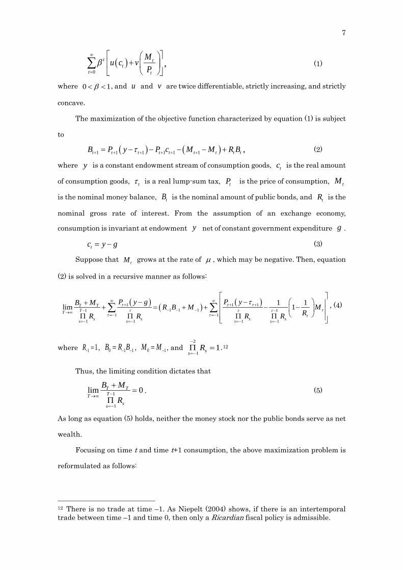
As mentioned above, this paper is motivated partly by several empirical facts

concerning the Japanese economy. The deflationary economy accompanied by monetary

expansion and zero rates of interest is a recent monetary phenomenon in Japan. As

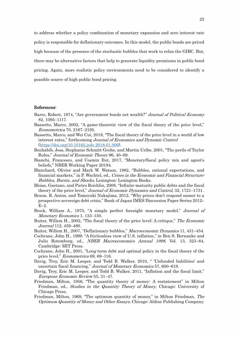
shown in Figure 1-1, the Marshallian k, which is defined as the ratio of outstanding Bank

of Japan (BoJ) notes to nominal gross domestic product (GDP), was quite stable up to

the early 1990s. That is, the price level was approximately proportional to the nominal

macroeconomic scale, and it was broadly determined according to the QTM. However,

when the call rates (the interbank money market rates) declined from just under 8% in

1990 to around 0.5% in 1995, the Marshallian k started to increase gradually, and the

increase has accelerated since the mid-1990s. The nominal rate of interest has been 9 Several papers, though not related to the FTPL, also provide potential reasons why public bonds are priced high despite a possible debt crisis. Sakuragawa and Sakuragawa (2016) demonstrate that public bonds are priced high, when public bonds serve as safe assets for those who strongly prefer domestic assets to foreign assets. Kobayashi and Ueda (2017) show that public bond yields are kept low despite a possible debt crisis, when a capital levy is imposed more mildly on public bonds than on private bonds at the time of a debt crisis. 10 Davig et al. (2010) share a similar structure of regime changes with this paper. Starting from active monetary policy and a stationary (passive) transfers process, their economy hits the fiscal limit as a consequence of a non-stationary (active) transfers process, and eventually enters the absorbing state of active monetary/passive transfers policy either directly or indirectly by way of passive monetary/active transfers policy.

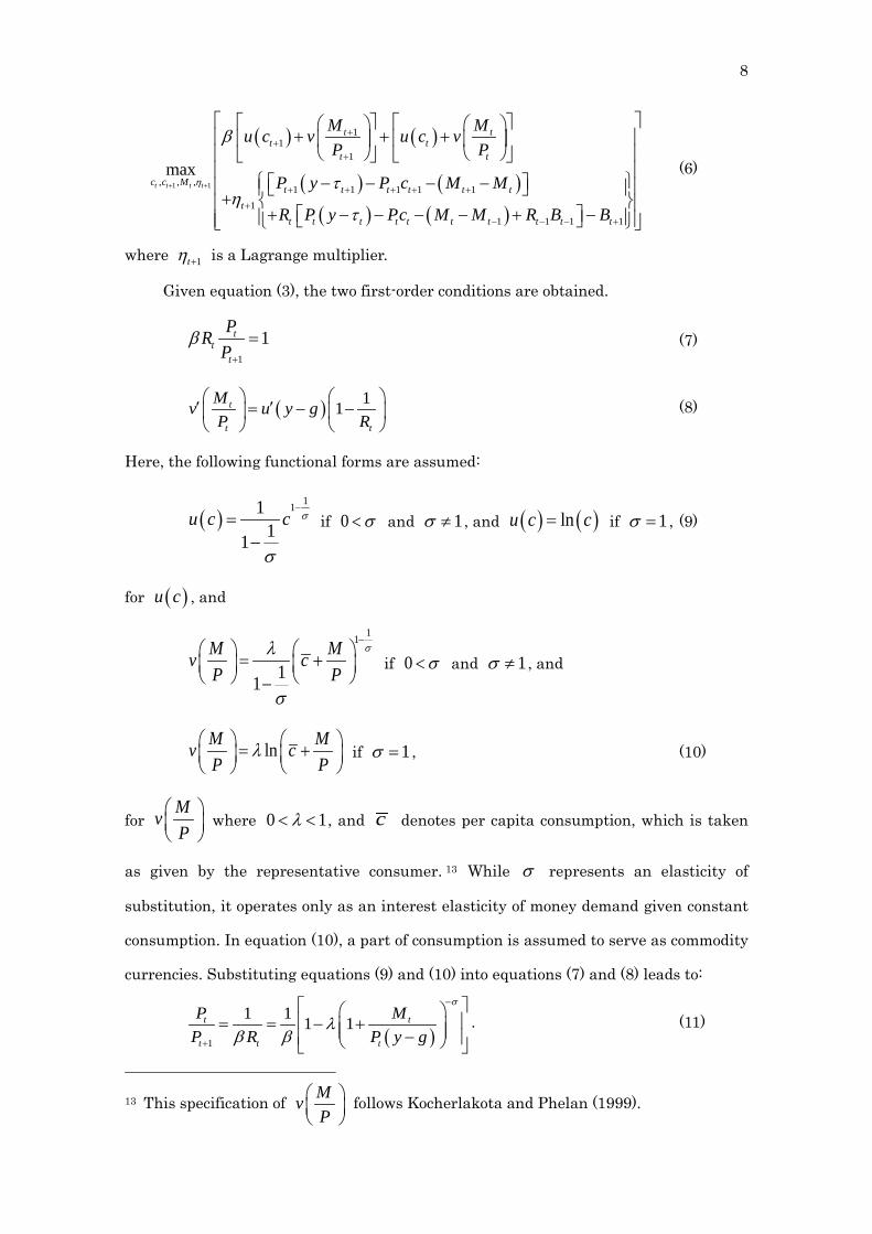
6

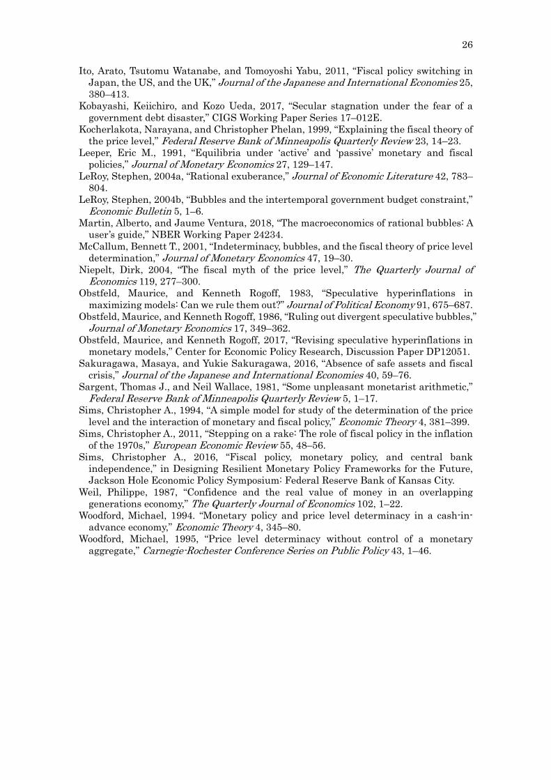
fairly close to zero since 1995. In addition, the public bonds accumulated more quickly

after the primary balance of the government’s general account became negative in the

mid-1990s. As shown in Figure 1-2, the ratio of public bonds to nominal GDP has

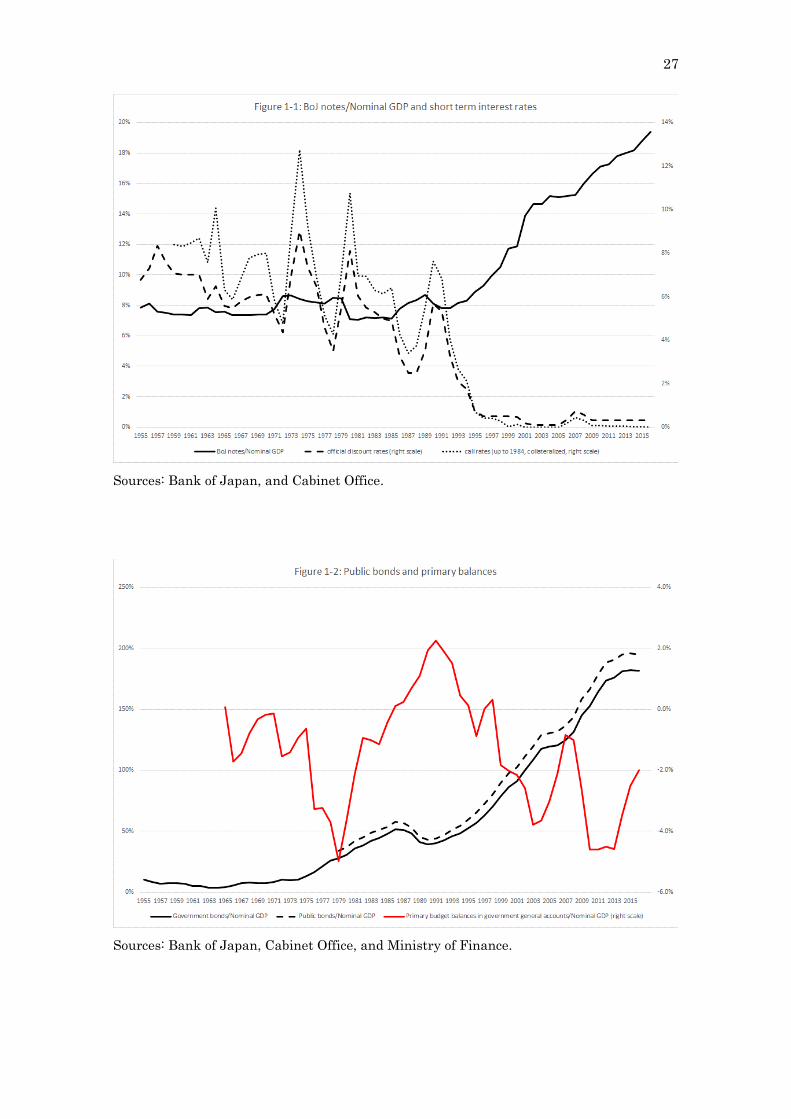
increased together with that of BoJ notes. As shown in Figure 1-3, however, a

deflationary trend started from the late 1990s.

In this paper, it is assumed that in the early 1990s, the Japanese economy began

to deviate from the long-run Ricardian regime with the QTM,11 and that the stochastic

bubbles work to relax the GIBC. If this were the case, then at a possible switching point

in the future, the bubbles would burst because of a heavy devaluation caused by a large,

one-off price increase. As implied by a calibration exercise that mimics the above-

described Japanese economy, the stochastic bubbles amount to around 40% of the real

valuation of public bonds, and the price level would jump by more than 200%

immediately after the economy switched to the Ricardian regime.

This paper is organized as follows. In Section 2, a monetary version of an exchange

economy is employed to analyze a Ricardian fiscal rule with the QTM and a non-

Ricardian fiscal rule with the FTPL separately. Section 3 presents a simple model in

which the regime with the FTPL probabilistically switches to the regime with the QTM.

In Section 4, several numerical examples shed light on some interpretations of the

current Japanese economy. Section 5 concludes.

2. Basic framework

2.1. Ricardian economy

In this section, a simple monetary model of exchange economy, proposed by Brock

(1975), Obstfeld and Rogoff (1983), and Kocherlakota and Phelan (1999), is presented as

a basic framework. The representative household has the following preference over

streams of consumption ( tc ) and the real money balance ( t

t

MP

):

11 According to Ito et al. (2011), the estimation result based on the net public bonds indicates that Japanese fiscal policy switched from a stationary Ricardian rule to a non-stationary non-Ricardian rule in the early 1990s.

7

( )0

t tt

t t

Mu c vP

β∞

=

+

∑ , (1)

where 0 1β< < , and u and v are twice differentiable, strictly increasing, and strictly

concave.

The maximization of the objective function characterized by equation (1) is subject

to

( ) ( )1 1 1 1 1 1t t t t t t t t tB P y P c M M R Bτ+ + + + + += − − − − + , (2)

where y is a constant endowment stream of consumption goods, tc is the real amount

of consumption goods, tτ is a real lump-sum tax, tP is the price of consumption, tM

is the nominal money balance, tB is the nominal amount of public bonds, and tR is the

nominal gross rate of interest. From the assumption of an exchange economy,

consumption is invariant at endowment net of constant government expenditure .

tc y g= − (3)

Suppose that tM grows at the rate of µ , which may be negative. Then, equation

(2) is solved in a recursive manner as follows:

( ) ( ) ( )1 1 11 1 11 1

1 11 1 1 1

1 1lim 1T TTT

s s s ss s s s

P y g P yB M R B M MRR R R R

τ τ τττ τ τ

τ τ τ

τ∞ ∞+ + +

− − −− −→∞=− =−

=− =− =− =−

− − + + = + + − − Π Π Π Π

∑ ∑ , (4)

where 1 1R− = , 0 1 1B R B− −= , 0 1M M −= , and 2

11ss

R−

=−Π = .12

Thus, the limiting condition dictates that

1

1

lim 0T TTT

ss

B M

R−→∞

=−

+=

Π. (5)

As long as equation (5) holds, neither the money stock nor the public bonds serve as net

wealth.

Focusing on time t and time t+1 consumption, the above maximization problem is

reformulated as follows:

12 There is no trade at time –1. As Niepelt (2004) shows, if there is an intertemporal trade between time –1 and time 0, then only a Ricardian fiscal policy is admissible.

y g

8

( ) ( )

( ) ( )( ) ( )

1 1

11

1

, , ,1 1 1 1 1

11 1 1 1

maxt t t t

t tt t

t t

c c Mt t t t t t

tt t t t t t t t t t

M Mu c v u c vP P

P y P c M M

R P y Pc M M R B B

η

β

τη

τ

+ +

++

+

+ + + + +

+

− − − +

+ + +

− − − − + + − − − − + −

(6)

where 1tη + is a Lagrange multiplier.

Given equation (3), the two first-order conditions are obtained.

(7)

( ) 11t

t t

Mv u y gP R

′ ′= − −

(8)

Here, the following functional forms are assumed:

( )111

11u c c σ

σ

−=

− if 0 σ< and 1σ ≠ , and ( ) ( )lnu c c= if 1σ = , (9)

for ( )u c , and

11

11

M Mv cP P

σλ

σ

− = + −

if 0 σ< and 1σ ≠ , and

lnM Mv cP P

λ = +

if 1σ = , (10)

for MvP

where 0 1λ< < , and c denotes per capita consumption, which is taken

as given by the representative consumer. 13 While σ represents an elasticity of

substitution, it operates only as an interest elasticity of money demand given constant

consumption. In equation (10), a part of consumption is assumed to serve as commodity

currencies. Substituting equations (9) and (10) into equations (7) and (8) leads to:

( )1

1 1 1 1t t

t t t

P MP R P y g

σ

λβ β

−

+

= = − + −

. (11)

13 This specification of MvP

follows Kocherlakota and Phelan (1999).

1

1tt

t

PRP

β+

=

9

Here, 0 1λ< < guarantees a positive 1

t

t

PP+

and a finite 1tP+

, even if ( )

t

t

MP y g−

converges to zero.

Let us begin with a Ricardian case where the QTM and Ricardian equivalence hold

jointly. Under the QTM, the price level and the money balance grow at the same rate µ .

Substituting 1

11

RtR

t

PP µ+

=+

into equation (11) leads to

1

tR µβ+

= , (12)

( )

11

11

R tt

MPy gσ

λ µµ β

=−+

− + −

, (13)

where RtP denotes the price of consumption goods in the Ricardian economy, and is

indeed proportional to the nominal amount of money balances tM .

Here, κ represents a constant Marshallian k, and is defined as ( )

tR

t

MP y g−

. Given

κ , λ is set as follows.

( )1 11

1σ

µ βλ κµ

+ −= +

+ (14)

The nominal primary budget balance is assumed to be proportional to the nominal

public bonds, net of seigniorage revenues 1t tM M −− :

( ) ( ) ( )1 1 1R

t t t t t tP g R B M Mτ γ− − −− = − − − , (15)

where 0 1γ< < . That is, seigniorage revenues are reimbursed as a lump-sum subsidy

to households. Hence, the nominal public bonds evolve according to

( ) ( )1 1 1

1 0

Rt t t t t t t

tt

B R B P g M M

B B

τ

γ γ− − −

−

= − − − −

= = (16)

That is, the public bonds are repaid over time by tax revenues. Thus, in the sense of

Woodford (1995), a fiscal rule specified by equation (15) is Ricardian.

Given the above fiscal rule, equation (5) holds as long as 11βγµ<

+.

10

( )0 00 0

1lim lim 0

11

TTTT

TT T

B MB M

γ µ γβµµ

β

→∞ →∞

+ + = + = + +

(17)

Note that Friedman’s rule with zero interest rates ( 1tR = ) cannot hold in this setup.

Substituting 1 0µ β= − < into equation (14) leads to 0λ = , which is inconsistent with

the parameter restriction 0 1λ< < . Nevertheless, if µ is close to 1 β− , but still

larger than 1 β− , then the economy approximately follows Friedman’s rule.14

This setup may yield a continuum of hyperinflationary or deflationary equilibria,

if the economy starts with an initial price other than given by equation (13). As

shown in Figure 2, the economy with 0 0RP P> is hyperinflationary; 1 1

1t

t

PP

β µλ

+ → > +−

,

0t

t

MP

→ , and 1 11tR µ

λ β+

→ >−

. Then, the terminal condition is derived as

( ) ( )0 0 0 00 01

0

1 1lim lim lim 0.

11

TT TT TT

T TT T Tss

B M B MB M

R

γ µ γ µ γβµµ

β

−→∞ →∞ →∞

=

+ + + + ≤ = + = + +Π

Thus, as long as 11βγµ<

+, equation (5) holds, and the hyperinflationary economy is

supported as a continuum of equilibria. On the other hand, the economy with 0 0RP P<

is deflationary; 1 1 1t

t

PP β+ → < , , and . Then, the terminal condition

associated with the money stock is derived as follows:

( )

( ) ( )001

00

1 1lim lim 1T

TTT T

ss

MM

RR

µµ−→∞ →∞

=

+= +ΛΠ

,

where ( )0 01ss

R R∞

=Λ = Π > Hence,

( ) 01

0

1lim

T

TTss

M

R

µ−→∞

=

+

Π diverges to infinity if 0µ > , it

14 Buiter and Sibert (2007) rigorously prove that Friedman’s rule with 1 0µ β= − < is inconsistent with the transversality condition.

0RP

t

t

MP

→∞ 1tR →

11

converges to ( )

0

0

MRΛ

( 0> ) if 0µ = , and it converges to zero if 1 0β µ− < < . That is,

a deflationary economy with monetary expansion or constant money stock is not

supported as a continuum of equilibria.

2.2. Non-Ricardian economy

As discussed in the introduction, the FTPL can be considered an equilibrium

selection device in the context of a continuum of hyperinflationary equilibria. Consider

a case where the initial price level 0NRP , which is determined by the FTPL, is larger than

given by equation (13). As equation (11) implies, with .

Suppose that the primary balance with seigniorage revenues never responds to the

nominal amount of public bonds.

( )NR NRt t t tP g P Mτ ε µ− = − , (18)

where and are positive. Again, seigniorage revenues are reimbursed as a lump-

sum subsidy to households. Thus, the real balance of the public bonds evolves according

to

( )1 1 1

1 .

NRt t t t t t

NRt t t

B R B P g M

R B P

τ µ

ε+ + +

+

= − − −

= − (19)

In the sense that the public bonds may not be repaid completely by tax revenues, a fiscal

rule specified by equation (18) is non-Ricardian.

Together with equation (7), equation (19) is rewritten as follows:

1

1

t tNR NR

t t

B BP P

β βε+

+

= + . (20)

Equation (20) is solved in a recursive manner.

10

00

1

01 0

1

00

lim

lim1

1lim1

T TNR NRT

T

NRTs TNR NRT s

s

TTNRT s

s

B BP P

P BP P

BR P

τ

τ

β ε β

βε ββ

βεβ

∞+

→∞=

−

→∞ =+

−

→∞ =

= +

= + Π −

= + Π −

∑

(21)

0RP 1 1

NRtNR

t

PP

µ+ > + 0 0NR RP P>

ε µ

12

As equation (19) implies, the nominal public bonds grow at a rate less than , as

long as 0ε > , 1tR > , and 0NRtP > . Thus, the second term of the third line in equation

(20) converges to zero, or

1

0

lim 0TTT

tt

B

R−→∞

=

=Π

. (22)

An essential aspect of equation (21) is that it cannot hold for any price 0NRP other

than a particular price. According to the FTPL, the initial price 0NRP is chosen such that

equation (21) may hold with 1

0

lim 0TTT

tt

B

R−→∞

=

=Π

, or

0

0 1NR

BP

βεβ

=−

. (23)

From (23) with ( )

0

0R

MP y g

κ =−

, the following condition is obtained.

0 0

0 0

11R

NR

P MP B

y g

β κεβ

−< → <

−

(24)

In this way, with inequality (24) satisfied, the FTPL as a selection device allows us

to choose a particular value for the initial price 0 0NR RP P> such that equation (23) holds.

3. Non-Ricardian economy as a deviation from the Ricardian economy

3.1. Three features of the model

In the previous section, the Ricardian economy with the QTM and the non-

Ricardian economy with the FTPL are explored separately. In this section, however, the

latter is considered a temporary, or at most a persistent, deviation from the former; with

a small probability, the non-Ricardian regime switches back into the Ricardian regime.

As demonstrated in this section, the setup with such a switching possibility allows space

for the stochastic bubbles that work to relax the GIBC (government’s intertemporal

budget constraint) during the deflationary non-Ricardian regime. Thus, the public bonds

are now backed not only by tax revenues in the current non-Ricardian regime before

switching and the future Ricardian regime after switching, but also by the stochastic

tB tR

13

bubbles during the former regime. In this way, the fiscal surpluses tentatively improve

with the stochastic bubbles despite the continuing budget deficits and, indeed, create a

deflationary pressure through a conventional mechanism of the FTPL. Immediately

after the economy switches to Ricardian, however, the bubbles burst because of a heavy

devaluation caused by a large, one-off increase in the price level, and the remaining

public bonds are repaid by tax revenues over time from then onward. In this way, a

government can operate a Ponzi scheme only if the deflationary non-Ricardian economy

continues.

In this section, the following three points are analyzed with adequate care. First,

there are potentially two cases in which the non-Ricardian economy switches to the

Ricardian economy. In one case, the non-Ricardian economy is hyperinflationary, and the

price level jumps down to the Ricardian level at switching. In the other case, the non-

Ricardian economy is deflationary, and the price level jumps up to the Ricardian level at

switching. During the non-Ricardian regime, the expected inflation (deflation) is formed

with consideration for such a downward (upward) price jump. There is a lower bound of

zero, but no ceiling on the price level, and excessively high prices cannot be consistent

with the expectation formation. Thus, the hyperinflationary non-Ricardian economy is

ruled out in this setup. Given the price level that eventually converges to zero, on the

other hand, the deflationary path remains consistent with the expectation formation.

Second, as long as the economy remains non-Ricardian, ex post deflations always

exceed expected deflations, thereby balancing a possible large price rise at switching.

Consequently, the nominal rate of interest, determined by real returns minus expected

deflations, is at least zero, whereas the actual nominal return, determined by real

returns minus ex post deflations, turns out to be negative. Such eventually negative

returns are responsible for the emergence of the stochastic bubbles that work to relax

the GIBC during the non-Ricardian regime. But, the representative consumer applies at

least zero nominal interest rates, thereby discounting to zero the expected present value

of the stochastic bubbles that emerge under the eventually negative nominal returns.

Accordingly, the public bonds with the stochastic bubbles never serve as net wealth even

in the deflationary non-Ricardian regime.

14

Third, the real valuation of public bonds depends on how large the stochastic

bubbles are in the GIBC, but it is completely independent of the present value of fiscal

surpluses that are generated during the non-Ricardian regime. In this FTPL

environment, the non-Ricardian economy is anchored eventually by the Ricardian

economy, and, sooner or later, the public bonds are financed ultimately by a heavy

devaluation when switching to the Ricardian regime, and tax revenues from then onward.

Thus, Ricardian equivalence still holds in this setup. Sims (2016) and others claim that

weaker fiscal discipline (a lower ε in this setup) helps to create more inflationary

pressures in the non-Ricardian regime. In this environment, however, the price level is

completely independent of how a non-Ricardian fiscal rule is implemented, and their

claim is not relevant in this model.

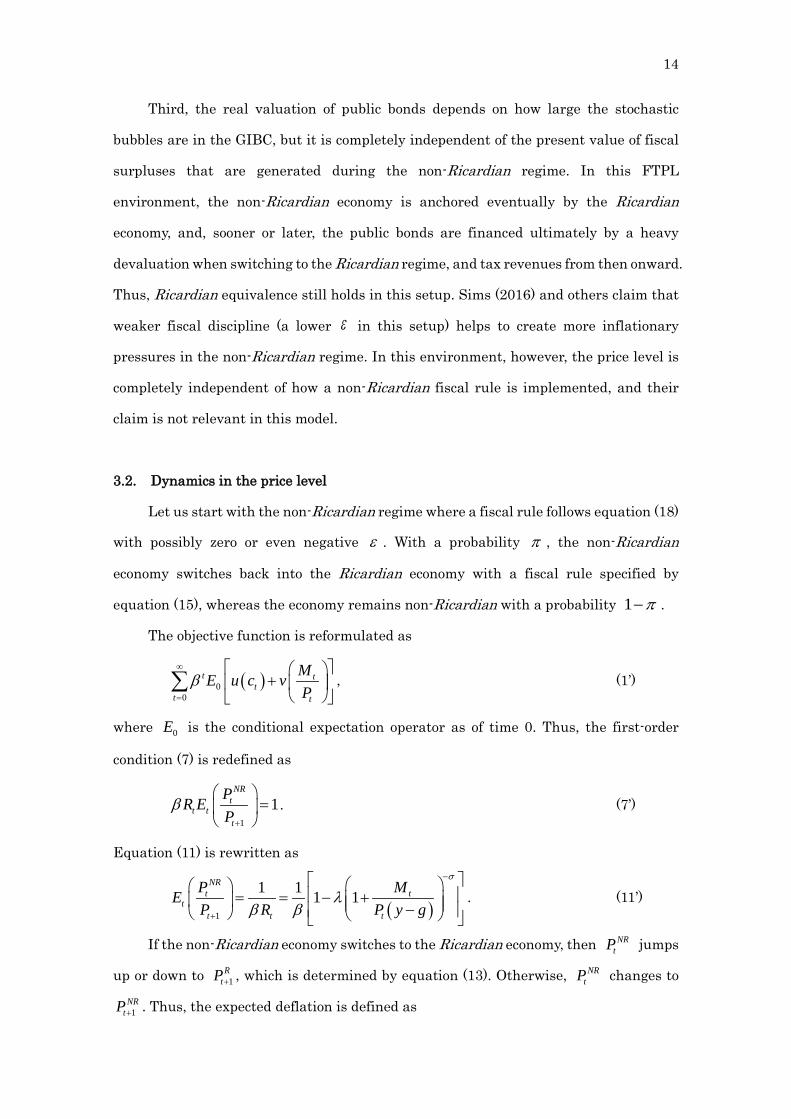
3.2. Dynamics in the price level

Let us start with the non-Ricardian regime where a fiscal rule follows equation (18)

with possibly zero or even negative ε . With a probability π , the non-Ricardian

economy switches back into the Ricardian economy with a fiscal rule specified by

equation (15), whereas the economy remains non-Ricardian with a probability 1 π− .

The objective function is reformulated as

( )00

t tt

t t

ME u c vP

β∞

=

+

∑ , (1’)

where 0E is the conditional expectation operator as of time 0. Thus, the first-order

condition (7) is redefined as

1

1NR

tt t

t

PR EP

β+

=

. (7’)

Equation (11) is rewritten as

( )1

1 1 1 1NR

t tt

t t t

P MEP R P y g

σ

λβ β

−

+

= = − + − . (11’)

If the non-Ricardian economy switches to the Ricardian economy, then NRtP jumps

up or down to 1R

tP+ , which is determined by equation (13). Otherwise, NRtP changes to

1NR

tP+ . Thus, the expected deflation is defined as

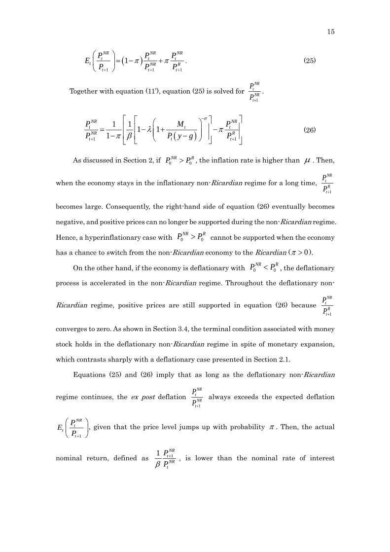
15

( )1 1 1

1NR NR NR

t t tt NR R

t t t

P P PEP P P

π π+ + +

= − +

. (25)

Together with equation (11’), equation (25) is solved for 1

NRtNR

t

PP+

.

( )1 1

1 1 1 11

NR NRt t tNR R

t t t

P M PP P y g P

σ

λ ππ β

−

+ +

= − + − − − (26)

As discussed in Section 2, if 0 0NR RP P> , the inflation rate is higher than µ . Then,

when the economy stays in the inflationary non-Ricardian regime for a long time, 1

NRt

Rt

PP+

becomes large. Consequently, the right-hand side of equation (26) eventually becomes

negative, and positive prices can no longer be supported during the non-Ricardian regime.

Hence, a hyperinflationary case with cannot be supported when the economy

has a chance to switch from the non-Ricardian economy to the Ricardian ( 0π > ).

On the other hand, if the economy is deflationary with , the deflationary

process is accelerated in the non-Ricardian regime. Throughout the deflationary non-

Ricardian regime, positive prices are still supported in equation (26) because 1

NRt

Rt

PP+

converges to zero. As shown in Section 3.4, the terminal condition associated with money

stock holds in the deflationary non-Ricardian regime in spite of monetary expansion,

which contrasts sharply with a deflationary case presented in Section 2.1.

Equations (25) and (26) imply that as long as the deflationary non-Ricardian

regime continues, the ex post deflation 1

NRtNR

t

PP+

always exceeds the expected deflation

1

NRt

tt

PEP+

, given that the price level jumps up with probability π . Then, the actual

nominal return, defined as 11 NRtNR

t

PPβ

+ , is lower than the nominal rate of interest

0 0NR RP P>

0 0NR RP P<

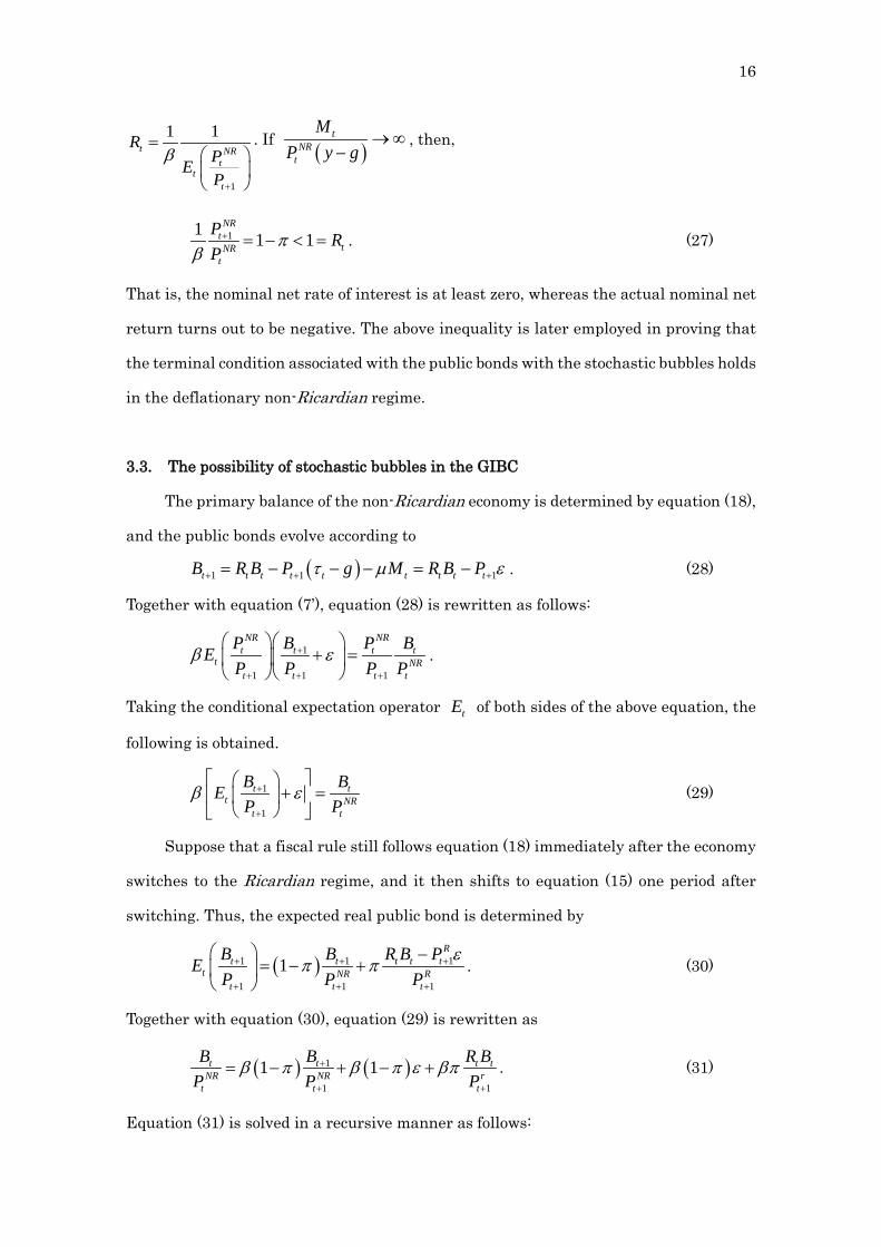
16

1

1 1t NR

tt

t

RPEP

β

+

=

. If ( )

tNR

t

MP y g

→∞−

, then,

11 1 1NR

ttNR

t

P RP

πβ

+ = − < = . (27)

That is, the nominal net rate of interest is at least zero, whereas the actual nominal net

return turns out to be negative. The above inequality is later employed in proving that

the terminal condition associated with the public bonds with the stochastic bubbles holds

in the deflationary non-Ricardian regime.

3.3. The possibility of stochastic bubbles in the GIBC

The primary balance of the non-Ricardian economy is determined by equation (18),

and the public bonds evolve according to

( )1 1 1t t t t t t t t tB R B P g M R B Pτ µ ε+ + += − − − = − . (28)

Together with equation (7’), equation (28) is rewritten as follows:

1

1 1 1

NR NRt t t t

t NRt t t t

P B P BEP P P P

β ε+

+ + +

+ =

.

Taking the conditional expectation operator tE of both sides of the above equation, the

following is obtained.

1

1

t tt NR

t t

B BEP P

β ε+

+

+ =

(29)

Suppose that a fiscal rule still follows equation (18) immediately after the economy

switches to the Ricardian regime, and it then shifts to equation (15) one period after

switching. Thus, the expected real public bond is determined by

( )1 1 1

1 1 1

1R

t t t t tt NR R

t t t

B B R B PEP P P

επ π+ + +

+ + +

−= − +

. (30)

Together with equation (30), equation (29) is rewritten as

( ) ( )1

1 1

1 1t t t tNR NR r

t t t

B B R BP P P

β π β π ε βπ+

+ +

= − + − + . (31)

Equation (31) is solved in a recursive manner as follows:

17

( ) ( ) ( )

( )( ) ( ) ( )

0

00 1

0 1

1 1 lim 1

11 lim 1 .

1 1

TT TNR R NRT

T

TT TR NRT

T

B R B BP P P

R B BP P

ττ τ τ

τ τ

ττ τ τ

τ τ

β π β π ε βπ β π

β π εβ π βπ β π

β π

∞

→∞= +

∞

→∞= +

= − − + + −

−

= + − + −− −

∑

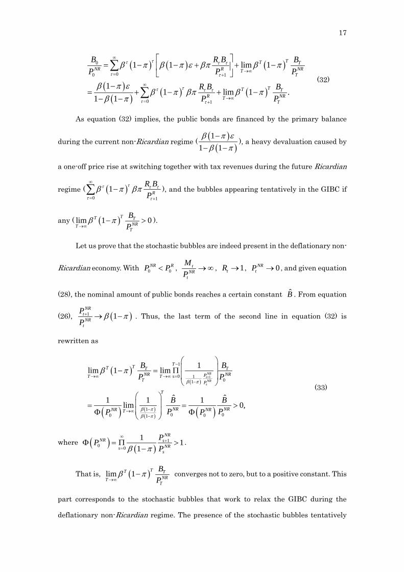
∑ (32)

As equation (32) implies, the public bonds are financed by the primary balance

during the current non-Ricardian regime ( ( )( )

11 1β π εβ π−

− −), a heavy devaluation caused by

a one-off price rise at switching together with tax revenues during the future Ricardian

regime ( ( )0 1

1 R

R BP

ττ τ τ

τ τ

β π βπ∞

= +

−∑ ), and the bubbles appearing tentatively in the GIBC if

any ( ( )lim 1 0TT TNRT

T

BP

β π→∞

− > ).

Let us prove that the stochastic bubbles are indeed present in the deflationary non-

Ricardian economy. With 0 0NR RP P< , t

NRt

MP

→∞ , 1tR → , 0NRtP → , and given equation

(28), the nominal amount of public bonds reaches a certain constant B̂ . From equation

(26), . Thus, the last term of the second line in equation (32) is

rewritten as

( )( )

( ) ( )( ) ( )

1

1

0 101

10 00 01

1lim 1 lim

ˆ ˆ1 1 1lim 0,

NRsNR

s

TTT T TNR NRPT T s

T P

T

NR NRNR NRT

B BP P

B BP PP P

β π

β πβ π

β π+

−

→∞ →∞ =−

−→∞−

− = Π

= = > Φ Φ

(33)

where ( ) ( )1

0 0

1 11

NRNR s

NRss

PPPβ π

∞+

=Φ = Π >

−.

That is, ( )lim 1 TT TNRT

T

BP

β π→∞

− converges not to zero, but to a positive constant. This

part corresponds to the stochastic bubbles that work to relax the GIBC during the

deflationary non-Ricardian regime. The presence of the stochastic bubbles tentatively

( )1 1NR

tNR

t

PP

β π+ → −

18

improves the fiscal surpluses, and it creates a deflationary pressure according to a

conventional mechanism of the FTPL. Thus, any initial price in the non-Ricardian

regime 0 0NR RP P< is consistent with equation (32) in the presence of the stochastic

bubbles ( ( )0 lim 1 TT TNRT

T

BP

β π→∞

< − < ∞ ). In this way, a government is able to operate a

Ponzi scheme only if the deflationary non-Ricardian economy continues. As shown in

Section 3.4, the terminal condition with the public bonds still holds in this case.

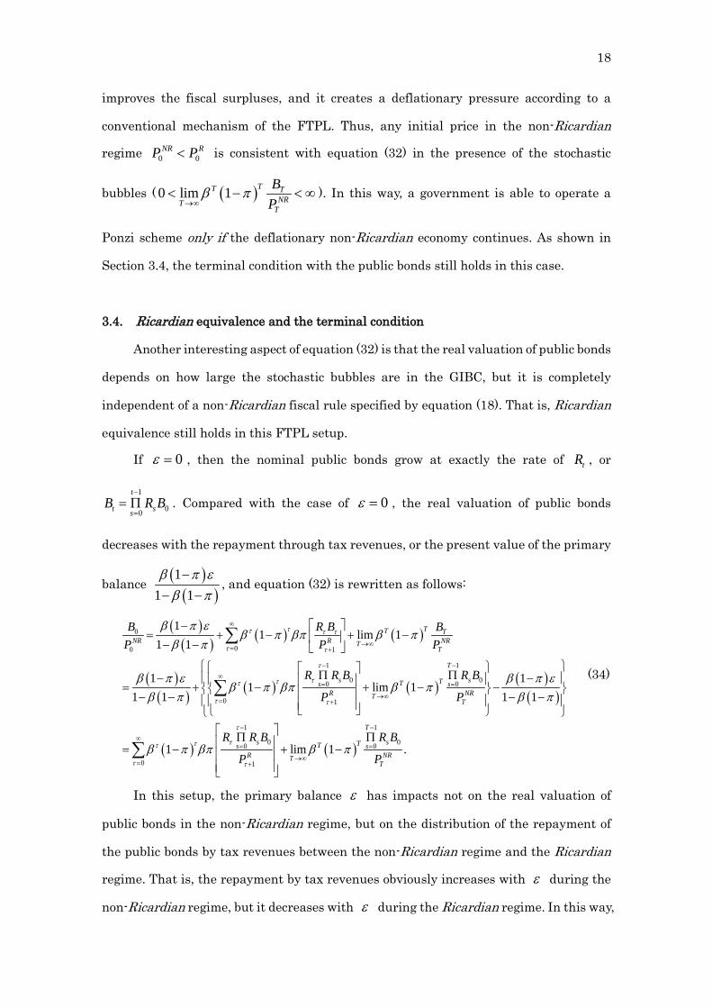
3.4. Ricardian equivalence and the terminal condition

Another interesting aspect of equation (32) is that the real valuation of public bonds

depends on how large the stochastic bubbles are in the GIBC, but it is completely

independent of a non-Ricardian fiscal rule specified by equation (18). That is, Ricardian

equivalence still holds in this FTPL setup.

If 0ε = , then the nominal public bonds grow at exactly the rate of tR , or

1

00

t

t ssB R B

−

== Π . Compared with the case of 0ε = , the real valuation of public bonds

decreases with the repayment through tax revenues, or the present value of the primary

balance ( )( )

11 1β π εβ π−

− −, and equation (32) is rewritten as follows:

( )( ) ( ) ( )

( )( ) ( ) ( ) ( )

( )

( )

0

00 1

1 1

0 00 0

0 1

0

0

11 lim 1

1 1

1 11 lim 1

1 1 1 1

1

TT TNR R NRT

T

T

s sTTs sR NRT

T

s

B R B BP P P

R R B R B

P P

R

ττ τ τ

τ τ

τ

τττ

τ τ

τττ

τ

β π εβ π βπ β π

β π

β π ε β π εβ π βπ β π

β π β π

β π βπ

∞

→∞= +

− −∞

= =

→∞= +

∞=

=

− = + − + − − −

Π Π− − = + − + − − − − − −

Π= −

∑

∑

∑ ( )1 1

0 00

1

lim 1 .

T

s sTT sR NRT

T

R B R B

P P

τ

τ

β π

− −

=

→∞+

Π + −

(34)

In this setup, the primary balance ε has impacts not on the real valuation of

public bonds in the non-Ricardian regime, but on the distribution of the repayment of

the public bonds by tax revenues between the non-Ricardian regime and the Ricardian

regime. That is, the repayment by tax revenues obviously increases with ε during the

non-Ricardian regime, but it decreases with ε during the Ricardian regime. In this way,

19

Ricardian equivalence still holds in this FTPL setup.

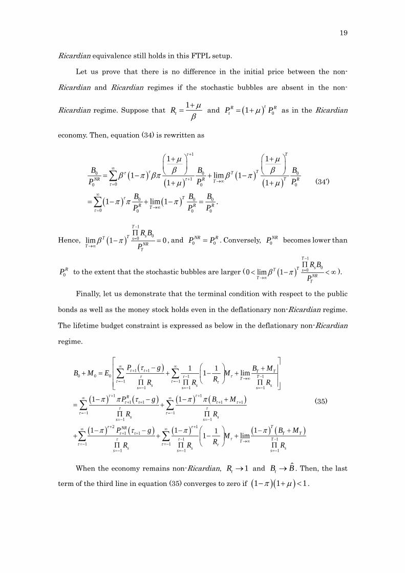
Let us prove that there is no difference in the initial price between the non-

Ricardian and Ricardian regimes if the stochastic bubbles are absent in the non-

Ricardian regime. Suppose that 1tR µ

β+

= and ( ) 01 tR RtP Pµ= + as in the Ricardian

economy. Then, equation (34) is rewritten as

( )( )

( )( )

( ) ( )

1

0 0 01

00 0 0

0 0 0

0 0 0 0

1 1

1 lim 11 1

1 lim 1 .

T

TTTNR R RT

TR R RT

B B BP P P

B B BP P P

τ

τττ

τ

τ

τ

µ µβ β

β π βπ β πµ µ

π π π

+

∞

+ →∞=

∞

→∞=

+ + = − + −+ +

= − + − =

∑

∑

(34’)

Hence, ( )1

00lim 1 0

T

sTT sNRT

T

R B

Pβ π

−

=

→∞

Π− = , and 0 0

NR RP P= . Conversely, 0NRP becomes lower than

0RP to the extent that the stochastic bubbles are larger ( ( )

1

000 lim 1

T

sTT sNRT

T

R B

Pβ π

−

=

→∞

Π< − < ∞ ).

Finally, let us demonstrate that the terminal condition with respect to the public

bonds as well as the money stock holds even in the deflationary non-Ricardian regime.

The lifetime budget constraint is expressed as below in the deflationary non-Ricardian

regime.

( )

( ) ( ) ( ) ( )

( ) ( ) ( )

1 10 0 0 1 1

1 11 1 1

1 11 1 1 1

1 11 1

2 11 1

11

1 11 lim

1 1

1 1

t T TTT

s s ss s s

Rt

s ss s

NRt

ss

P g B MB M E MRR R R

P g B M

R R

P g

R

τττ τ

τ τ τ

τ ττ τ τ

τ ττ τ

τ ττ

ττ

τ

π π τ π π

π τ π

∞ ∞+ +

− −→∞=− =−

=− =− =−

+ +∞ ∞+ + + +

=− =−=− =−

+ +∞+ +

=−=−

− + + = + − + Π Π Π

− − − += +

Π Π

− − −+ +

Π Π

∑ ∑

∑ ∑

∑ ( ) ( )1 1

11 1

111 limT

T TTT

s ss s

B MM

RR Rττ

τ τ

π∞

− −→∞=−

=− =−

− + − +

Π∑

(35)

When the economy remains non-Ricardian, 1tR → and ˆtB B→ . Then, the last

term of the third line in equation (35) converges to zero if ( )( )1 1 1π µ− + < .

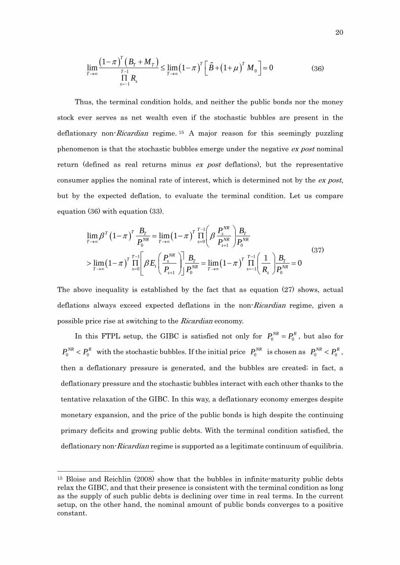
20

( ) ( ) ( ) ( ) 01

1

1 ˆlim lim 1 1 0T

T TT TTT T

ss

B MB M

R

ππ µ−→∞ →∞

=−

− + ≤ − + + = Π

(36)

Thus, the terminal condition holds, and neither the public bonds nor the money

stock ever serves as net wealth even if the stochastic bubbles are present in the

deflationary non-Ricardian regime. 15 A major reason for this seemingly puzzling

phenomenon is that the stochastic bubbles emerge under the negative ex post nominal

return (defined as real returns minus ex post deflations), but the representative

consumer applies the nominal rate of interest, which is determined not by the ex post,

but by the expected deflation, to evaluate the terminal condition. Let us compare

equation (36) with equation (33).

( ) ( )

( ) ( )

1

00 1 0

1 1

0 11 0 0

lim 1 lim 1

1lim 1 lim 1 0

NRTT TT sT TNR NR NRT T s

s

NRT TT Ts T Tt NR NRT s T s

s s

PB BP P P

P B BEP P R P

β π π β

π β π

−

→∞ →∞ =+

− −

→∞ = →∞ =−+

− = − Π

> − Π = − Π =

(37)

The above inequality is established by the fact that as equation (27) shows, actual

deflations always exceed expected deflations in the non-Ricardian regime, given a

possible price rise at switching to the Ricardian economy.

In this FTPL setup, the GIBC is satisfied not only for 0 0NR RP P= , but also for

0 0NR RP P< with the stochastic bubbles. If the initial price 0

NRP is chosen as 0 0NR RP P< ,

then a deflationary pressure is generated, and the bubbles are created; in fact, a

deflationary pressure and the stochastic bubbles interact with each other thanks to the

tentative relaxation of the GIBC. In this way, a deflationary economy emerges despite

monetary expansion, and the price of the public bonds is high despite the continuing

primary deficits and growing public debts. With the terminal condition satisfied, the

deflationary non-Ricardian regime is supported as a legitimate continuum of equilibria.

15 Bloise and Reichlin (2008) show that the bubbles in infinite-maturity public debts relax the GIBC, and that their presence is consistent with the terminal condition as long as the supply of such public debts is declining over time in real terms. In the current setup, on the other hand, the nominal amount of public bonds converges to a positive constant.

21

Such a seemingly paradoxical phenomenon is sustained only by the possibility that the

non-Ricardian economy sooner or later reverts to the Ricardian world. Once it switches

to the Ricardian, the economy experiences a sudden and difficult turnaround phase

before everything returns to normal. That is, the bubbles burst because of a significant

devaluation caused by a one-off price rise at the switching point, before the remaining

public bonds are repaid over time by tax revenues, and the prices increase with

monetary expansion according to the QTM.

4. Some numerical examples and calibration exercises

In this section, several numerical examples are presented first to illuminate the

general properties of the deflationary non-Ricardian regime, and then to demonstrate

how this model mimics the current Japanese economy.

4.1. Numerical examples

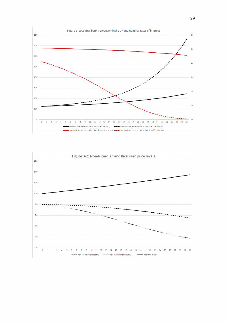
Let us begin with the case where 0.96β = , 0.01µ = , 0.1κ = , 0.05π = , σ is

either 1 or 0.1, and λ is determined by equation (14). Here, ( )( )1 1 1µ π+ − < is

satisfied. In terms of the initial conditions, 100y g− = , ε is set at zero, 0 100M = ,

and 0 100B = . Given this set of parameters, 0 10RP = . Then, any initial price 0NRP less

than 10 is consistent with the deflationary non-Ricardian economy. Thus, 0NRP is set at

8.

As shown in Figure 3-1, the nominal net rate of interest ( 1tR − ) decreases mildly

from 5.1% to 4.6% over 30 years if σ is 1, but it declines substantially from 4.1% to

almost zero if the interest elasticity of money demand is quite low ( 0.1σ = ). The relative

size of money stock or the Marshallian k (( )

tNR

t

MP y g−

) increases from 12.5% to 24.5 % if

1σ = , and from 12.5% to 75.8% if 0.1σ = . Figure 3-2 shows that the price level NRtP

declines despite monetary expansion in the non-Ricardian regime, whereas RtP grows

at the rate of 1% in the Ricardian regime. With 0.1σ = , for example, 19 4.1NRP = in year

19, but 20 12.2RP = in year 20. Thus, if the economy switches back into the Ricardian

regime in year 20, then the price level jumps by around 200%. As a consequence of this

22

one-off large price increase, the public bonds are heavily devalued when switching to the

Ricardian economy.

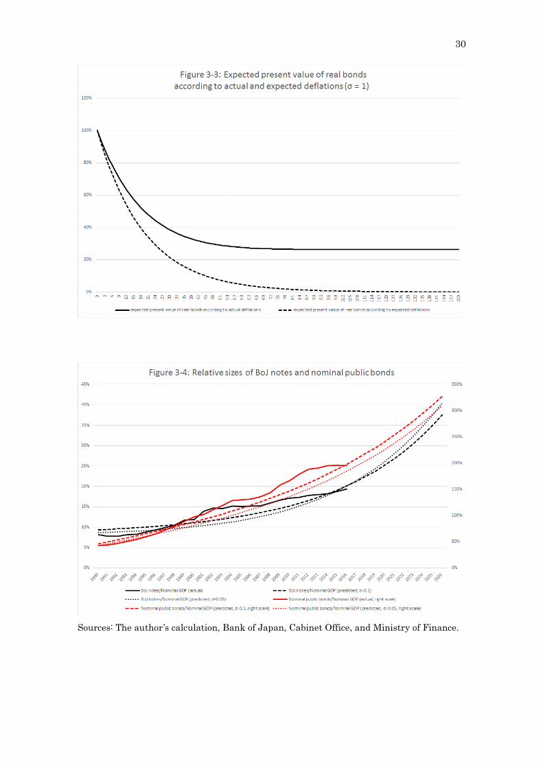
As Figure 3-3 demonstrates, the expected present value of the future public bonds,

which is discounted according to the actual nominal return ( ( )1

001

T

sTT sNR

T

R B

Pβ π

−

=Π

− in

equation (34)), converges to a positive constant, whereas the value that is discounted

according to the nominal rate of interest ( ( )1

10

11TT T

NRss

BR P

π−

=−

− Π

in equation (35))

converges to zero. The share of the stochastic bubbles amounts to 26% of the real

valuation of public bonds ( 0

0NR

BP

) under the above assumption. This numerical example

demonstrates that the stochastic bubbles are present in the GIBC, but that they never

constitute any net wealth even in the deflationary non-Ricardian regime.

4.2. Calibration exercises

Next, let us present calibration exercises that mimic the recent Japanese economy.

In particular, the exercises are constructed such that the relative amounts of Bank of

Japan notes (BoJ notes) and public bonds during the 1990-2016 period can be matched

approximately with those predicted by the model.

A set of parameters is determined as follows. β is set at close to 1 or 0.99 to yield

low nominal rates of interest, σ is either 0.1 or 0.05 to reproduce a substantial decrease

in interest rates over time, κ is 0.078, which is equal to the 1980–1995 average

Marshallian k (( )

t

t

MEP y g −

), µ is 0.033, which corresponds to the 2000–2016

average growth of BoJ notes, and λ is determined by equation (14). Given 100y g− = ,

the primary balance ε is set at –0.029, which is obtained from the 2000–2016 average

ratio of the primary balance of the government’s general account to nominal GDP. Setting

1990 as the starting year, 1990M is standardized as 100, and 1990B is set at 493, because

the outstanding BoJ notes and public bonds amounted to 40 trillion yen and 196 trillion

yen, respectively, in 1990. Given the above set of parameters, 1990RP is computed as 12.8;

23

then, the initial price ( 1990NRP ) needs to be less than 12.8 to present a deflationary case

Being consistent with ( )( )1 0.033 1 1π+ − < , π is set at 0.04. 1990NRP is set at 10.7

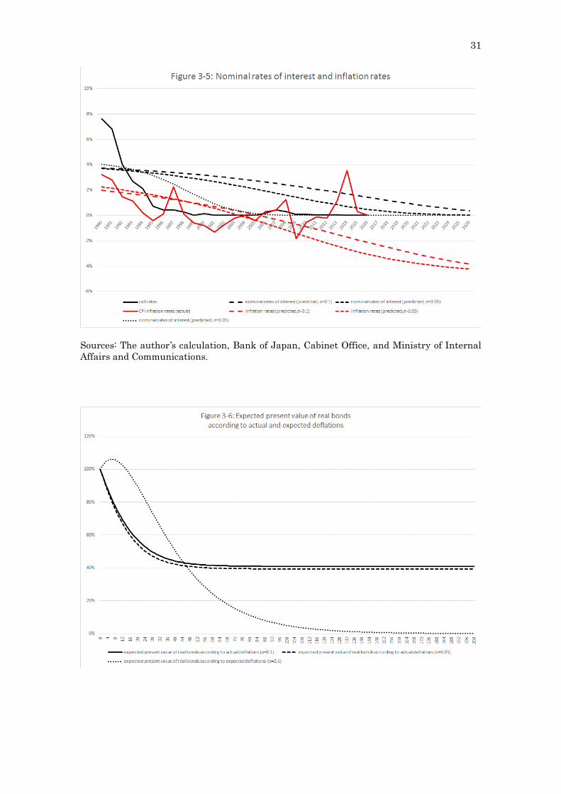
(<12.8) for 0.1σ = , and at 11.6 (<12.8) for 0.05σ = . As shown in Figure 3-4, the

predictions and observations are matched approximately in the years of 1990–2016. As

Figure 3-5 shows, the predicted inflation rate captures the actual trend except in year

2014 when the consumption tax rate was raised from 5% to 8%. If σ is 0.05, the

predicted nominal rate of interest is close to zero in the 2010s, but it still declines a little

more slowly than the observations did. If σ is set at an unusually low value or 0.01

together with 1990 12.7NRP = ,16 then the predicted rate of interest approaches zero in the

early 2000s.

What would happen to the Japanese economy if the regime switched from non-

Ricardian to Ricardian? As shown in Figure 3-6, the stochastic bubbles amount to about

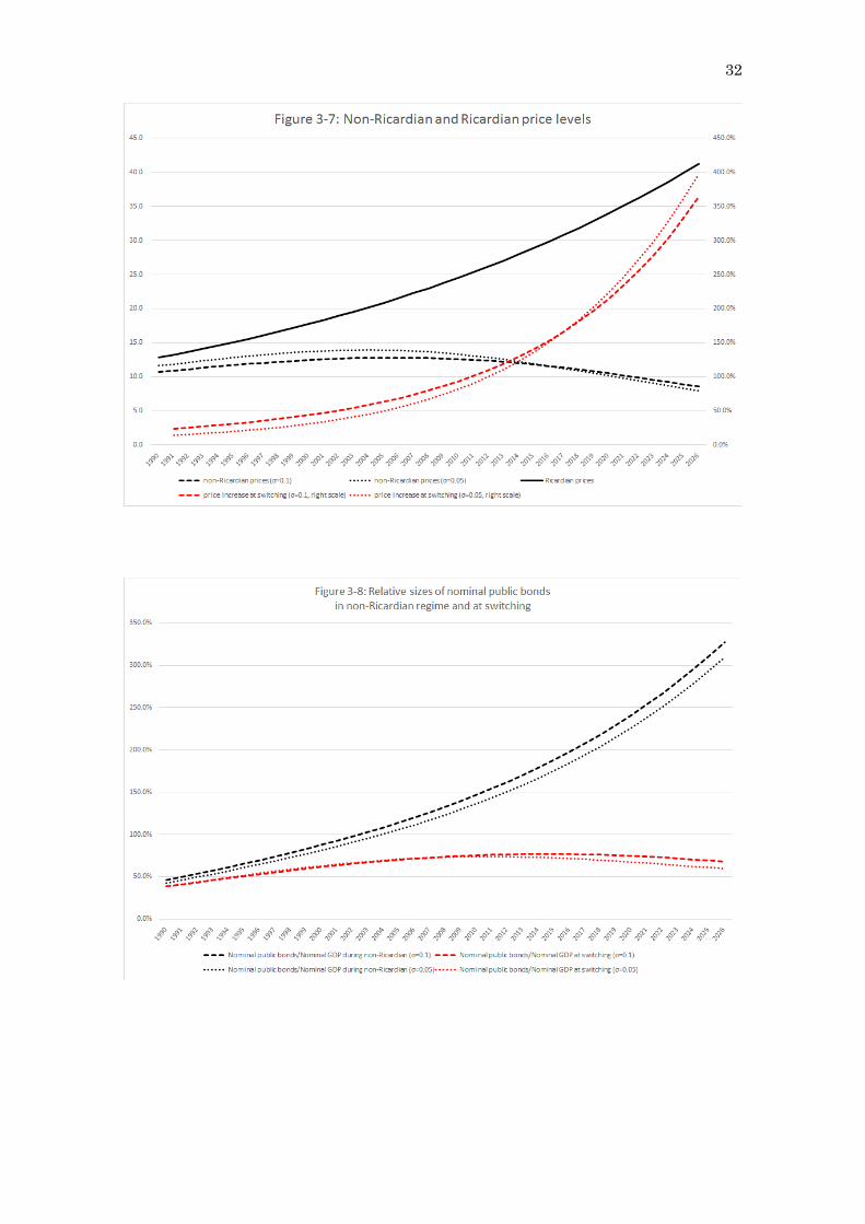
40% of the real valuation of public bonds in this calibration exercise. Figure 3-7

demonstrates that a difference between NRtP and R

tP becomes larger and larger as

time goes on. For example, consider 0.1σ = , 2019 10.8NRP = , and 2020 34.0RP = . Thus, if the

economy switched back to Ricardian in 2020, then the price level would jump by more

than 200%, the accumulated nominal bonds would be devalued heavily from 230% to

75% in terms of the ratio to nominal GDP, the Marshallian k would fall from 25% to 8%

( κ= ), and the nominal rate of interest would rise suddenly from near-zero rates to more

than 4% ( 1 µβ+

= ). If the switching occurred in 2026, the price level would jump by 364%,

and the relative amount of public bonds would reduce dramatically from 311% to 68%.

5. Conclusion

A deflationary economy with monetary expansion and growing public debts under

near-zero rates of interest is hard to reconcile with the implications from standard

monetary models with the QTM, and it is also difficult to justify using alternative

16 When 0.01σ = and 1990 12.7NRP = , the predictions and observations match approximately in terms of the relative amounts of BoJ notes and public bonds for the 1990–2016 series.

24

monetary models with the FTPL. However, if the latter models are viewed as a temporary,

or at most a persistent, deviation from the former, then a deflationary economy with

monetary expansion can be characterized as a legitimate continuum of equilibria. Given

such probabilistic switching from the FTPL to the QTM, the stochastic bubbles may

emerge in a deflationary environment, thereby relaxing the GIBC (government’s

intertemporal budget constraint), but they burst because of a heavy devaluation caused

by a large, one-off increase in the price level at switching. In this way, a government is

able to operate a Ponzi scheme only in the deflationary non-Ricardian economy.

In terms of policy implications, Ricardian equivalence still holds in this FTPL setup.

The price level decreases with the size of the stochastic bubbles, but it is completely

independent of how a non-Ricardian fiscal policy is implemented. A major reason for this

is that the non-Ricardian economy is eventually anchored by the Ricardian economy, and

the public bonds accumulated under the continuing primary deficits are sooner or later

repaid by a heavy devaluation at switching, and by a Ricardian fiscal policy after

switching. Given this implication, weaker (stronger) fiscal discipline never generates

more inflationary (deflationary) pressures; thus, a fiscal policy may not be employed as

an instrument to control the price level.

There are also positive implications from this model. A transition from the non-

Ricardian regime to the Ricardian regime is never smooth, but rather discontinuous in

terms of the price level, the relative amounts of public bonds and money stock, and the

nominal rate of interest, in the presence of the bubbles that eventually burst. Under this

scenario, it is predicted that the deflationary Japanese economy accompanied by

monetary expansion and growing public debts–which has been often viewed as the new

normal in practical policy debates–will experience a sudden and difficult reversal before

everything returns to the old normal.

There are not a few policy issues that remain unresolved in this paper. Here, the

non-Ricardian regime with monetary expansion involves an equilibrium in which a

combination of mild inflations and non-zero interest rates holds under the QTM. Why is

a particular path picked up among equilibria with deflations and declining interest rates

in spite of this fact? More sophisticated policy rules need to be taken into consideration

25

to address whether a policy combination of monetary expansion and zero interest rate

policy is responsible for deflationary outcomes. In this model, the public bonds are priced

high because of the presence of the stochastic bubbles that work to relax the GIBC. But,

there may be alternative factors that help to generate liquidity premiums in public bond

pricing. Again, more realistic policy environments need to be considered to identify a

possible source of high public bond pricing.

References: Barro, Robert, 1974, “Are government bonds net wealth?” Journal of Political Economy

82, 1095–1117. Bassetto, Marco, 2002, “A game-theoretic view of the fiscal theory of the price level,”

Econometrica 70, 2167–2195. Bassetto, Marco, and Wei Cui, 2018, “The fiscal theory of the price level in a world of low

interest rates,” forthcoming Journal of Economics and Dynamic Control (https://doi.org/10.1016/j.jedc.2018.01.006).

Benhabib, Jess, Stephanie Schmitt-Grohe, and Martin Uribe, 2001, “The perils of Taylor Rules,” Journal of Economic Theory 96, 40–69.

Bianchi, Francesco, and Cosmin Ilut, 2017, “Monetary/fiscal policy mix and agent’s beliefs,” NBER Working Paper 20194.

Blanchard, Olivier and Mark W. Watson, 1982, “Bubbles, rational expectations, and financial markets,” in P. Wachtel, ed., Crises in the Economic and Financial Structure: Bubbles, Bursts, and Shocks, Lexington: Lexington Books.

Bloise, Gaetano, and Pietro Reichlin, 2008, “Infinite-maturity public debts and the fiscal theory of the price level,” Journal of Economic Dynamics and Control, 32, 1721–1731.

Braun. R. Anton, and Tomoyuki Nakajima, 2012, “Why prices don’t respond sooner to a prospective sovereign debt crisis,” Bank of Japan IMES Discussion Paper Series 2012–E–2.

Brock, William A., 1975, “A simple perfect foresight monetary model,” Journal of Monetary Economics 1, 133–150.

Buiter, Willem H., 2002, “The fiscal theory of the price level: A critique,” The Economic Journal 112, 459–480.

Buiter, Willem H., 2007, “Deflationary bubbles,” Macroeconomic Dynamics 11, 431–454. Cochrane, John H., 1999. “A frictionless view of U.S. inflation,” in Ben S. Bernanke and

Julio Rotemberg, ed., NBER Macroeconomics Annual 1998, Vol. 13, 323–84, Cambridge: MIT Press.

Cochrane, John H., 2001, “Long-term debt and optimal policy in the fiscal theory of the price level,” Econometrica 69, 69–116.

Davig, Troy, Eric M. Leeper, and Todd B. Walker, 2010, “ ‘Unfunded liabilities’ and uncertain fiscal financing,” Journal of Monetary Economics 57, 600–619.

Davig, Troy, Eric M. Leeper, and Todd B. Walker, 2011, “Inflation and the fiscal limit,” European Economic Review 55, 31–47.

Friedman, Milton, 1956, “The quantity theory of money: A restatement” in Milton Friedman, ed., Studies in the Quantity Theory of Money, Chicago: University of Chicago Press.

Friedman, Milton, 1969, “The optimum quantity of money,” in Milton Friedman, The Optimum Quantity of Money and Other Essays, Chicago: Aldine Publishing Company.

26 Ito, Arato, Tsutomu Watanabe, and Tomoyoshi Yabu, 2011, “Fiscal policy switching in

Japan, the US, and the UK,” Journal of the Japanese and International Economies 25, 380–413.

Kobayashi, Keiichiro, and Kozo Ueda, 2017, “Secular stagnation under the fear of a government debt disaster,” CIGS Working Paper Series 17–012E.

Kocherlakota, Narayana, and Christopher Phelan, 1999, “Explaining the fiscal theory of the price level,” Federal Reserve Bank of Minneapolis Quarterly Review 23, 14–23.

Leeper, Eric M., 1991, “Equilibria under ‘active’ and ‘passive’ monetary and fiscal policies,” Journal of Monetary Economics 27, 129–147.

LeRoy, Stephen, 2004a, “Rational exuberance,” Journal of Economic Literature 42, 783–804.

LeRoy, Stephen, 2004b, “Bubbles and the intertemporal government budget constraint,” Economic Bulletin 5, 1–6.

Martin, Alberto, and Jaume Ventura, 2018, “The macroeconomics of rational bubbles: A user’s guide,” NBER Working Paper 24234.

McCallum, Bennett T., 2001, “Indeterminacy, bubbles, and the fiscal theory of price level determination,” Journal of Monetary Economics 47, 19–30.

Niepelt, Dirk, 2004, “The fiscal myth of the price level,” The Quarterly Journal of Economics 119, 277–300.

Obstfeld, Maurice, and Kenneth Rogoff, 1983, “Speculative hyperinflations in maximizing models: Can we rule them out?” Journal of Political Economy 91, 675–687.

Obstfeld, Maurice, and Kenneth Rogoff, 1986, “Ruling out divergent speculative bubbles,” Journal of Monetary Economics 17, 349–362.

Obstfeld, Maurice, and Kenneth Rogoff, 2017, “Revising speculative hyperinflations in monetary models,” Center for Economic Policy Research, Discussion Paper DP12051.

Sakuragawa, Masaya, and Yukie Sakuragawa, 2016, “Absence of safe assets and fiscal crisis,” Journal of the Japanese and International Economies 40, 59–76.

Sargent, Thomas J., and Neil Wallace, 1981, “Some unpleasant monetarist arithmetic,” Federal Reserve Bank of Minneapolis Quarterly Review 5, 1–17.

Sims, Christopher A., 1994, “A simple model for study of the determination of the price level and the interaction of monetary and fiscal policy,” Economic Theory 4, 381–399.

Sims, Christopher A., 2011, “Stepping on a rake: The role of fiscal policy in the inflation of the 1970s,” European Economic Review 55, 48–56.

Sims, Christopher A., 2016, “Fiscal policy, monetary policy, and central bank independence,” in Designing Resilient Monetary Policy Frameworks for the Future, Jackson Hole Economic Policy Symposium: Federal Reserve Bank of Kansas City.

Weil, Philippe, 1987, “Confidence and the real value of money in an overlapping generations economy,” The Quarterly Journal of Economics 102, 1–22.

Woodford, Michael, 1994. “Monetary policy and price level determinacy in a cash-in-advance economy,” Economic Theory 4, 345–80.

Woodford, Michael, 1995, “Price level determinacy without control of a monetary aggregate,” Carnegie-Rochester Conference Series on Public Policy 43, 1–46.

27

Sources: Bank of Japan, and Cabinet Office.

Sources: Bank of Japan, Cabinet Office, and Ministry of Finance.

28

Sources: Cabinet Office and Ministry of Internal Affairs and Communications.

0

Figure 2: Price levels and inflation rates

29

30

Sources: The author’s calculation, Bank of Japan, Cabinet Office, and Ministry of Finance.

31

Sources: The author’s calculation, Bank of Japan, Cabinet Office, and Ministry of Internal Affairs and Communications.

32