On the Performance of Tensor Methods for Solving Ill ... the Performance of Tensor Methods for Solving Ill-conditioned Problems Brett W. Bader and Robert B. Schnabel ... at the solution.Published

SANDIA REPORTSAND2004-1944Unlimited ReleasePrinted September 2004

On the Performance of TensorMethods for Solving Ill-conditionedProblems

Brett W. Bader and Robert B. Schnabel

Prepared bySandia National LaboratoriesAlbuquerque, New Mexico 87185 and Livermore, California 94550

Sandia is a multiprogram laboratory operated by Sandia Corporation,a Lockheed Martin Company, for the United States Department of Energy’sNational Nuclear Security Administration under Contract DE-AC04-94-AL85000.

Approved for public release; further dissemination unlimited.

Issued by Sandia National Laboratories, operated for the United States Department ofEnergy by Sandia Corporation.

NOTICE: This report was prepared as an account of work sponsored by an agency ofthe United States Government. Neither the United States Government, nor any agencythereof, nor any of their employees, nor any of their contractors, subcontractors, or theiremployees, make any warranty, express or implied, or assume any legal liability or re-sponsibility for the accuracy, completeness, or usefulness of any information, appara-tus, product, or process disclosed, or represent that its use would not infringe privatelyowned rights. Reference herein to any specific commercial product, process, or serviceby trade name, trademark, manufacturer, or otherwise, does not necessarily constituteor imply its endorsement, recommendation, or favoring by the United States Govern-ment, any agency thereof, or any of their contractors or subcontractors. The views andopinions expressed herein do not necessarily state or reflect those of the United StatesGovernment, any agency thereof, or any of their contractors.

Printed in the United States of America. This report has been reproduced directly fromthe best available copy.

Available to DOE and DOE contractors fromU.S. Department of EnergyOffice of Scientific and Technical InformationP.O. Box 62Oak Ridge, TN 37831

Telephone: (865) 576-8401Facsimile: (865) 576-5728E-Mail: [email protected] ordering: http://www.doe.gov/bridge

Available to the public fromU.S. Department of CommerceNational Technical Information Service5285 Port Royal RdSpringfield, VA 22161

Telephone: (800) 553-6847Facsimile: (703) 605-6900E-Mail: [email protected] ordering: http://www.ntis.gov/ordering.htm

SAND2004-1944Unlimited Release

Printed September 2004

On the Performance of Tensor Methodsfor Solving Ill-conditioned Problems

Brett W. BaderComputational Sciences Department

Sandia National LaboratoriesP.O. Box 5800, MS-0316

Albuquerque, NM 87185-0316

Robert B. SchnabelDepartment of Computer ScienceUniversity of Colorado at Boulder

Boulder, CO 80309-0040

Abstract

This paper investigates the performance of tensor methods for solving small-and large-scale systems of nonlinear equations where the Jacobian matrix atthe root is ill-conditioned or singular. This condition occurs on many classesof problems, such as identifying or approaching turning points in path fol-lowing problems. The singular case has been studied more than the highlyill-conditioned case, for both Newton and tensor methods. It is known thatNewton-based methods do not work well with singular problems because theyconverge linearly to the solution and, in some cases, with poor accuracy. Onthe other hand, direct tensor methods have performed well on singular prob-lems and have superlinear convergence on such problems under certain condi-tions. This behavior originates from the use of a special, restricted form of thesecond-order term included in the local tensor model that provides informationlacking in a (nearly) singular Jacobian. With several implementations avail-able for large-scale problems, tensor methods now are capable of solving largerproblems. We compare the performance of tensor methods and Newton-basedmethods for both small- and large-scale problems over a range of conditionings,from well-conditioned to ill-conditioned to singular. Previous studies with ten-sor methods only concerned the ends of this spectrum. Our results show thattensor methods are increasingly superior to Newton-based methods as the prob-lem grows more ill-conditioned.

3

Acknowledgment

The work of both authors was supported in part by Air Force Office of ScientificResearch grant F49620-00-1-0162 and Army Research Office grant DAAG55-98-1-0176 while in the Department of Computer Science at the University of Colorado,Boulder.

While at Sandia, the first author also received support from DOE’s Office ofScience MICS program and Sandia’s Laboratory Directed Research and Developmentprogram under LDRD 04-1024.

4

Contents

1 Introduction . . . . . . . . . . . . . . . . . . . . . . . . . . . . . . . . . . . . . . . . . . . . . . . . . . . . 7

2 Algorithms . . . . . . . . . . . . . . . . . . . . . . . . . . . . . . . . . . . . . . . . . . . . . . . . . . . . . 92.1 Standard Methods . . . . . . . . . . . . . . . . . . . . . . . . . . . . . . . . . . . . . . . . . . . 92.2 Tensor methods . . . . . . . . . . . . . . . . . . . . . . . . . . . . . . . . . . . . . . . . . . . . . 92.3 Newton-Krylov methods . . . . . . . . . . . . . . . . . . . . . . . . . . . . . . . . . . . . . . 102.4 Tensor-Krylov methods . . . . . . . . . . . . . . . . . . . . . . . . . . . . . . . . . . . . . . . 112.5 Tensor-GMRES method . . . . . . . . . . . . . . . . . . . . . . . . . . . . . . . . . . . . . . . 12

3 Numerical experiments on ill-conditioned problems. . . . . . . . . . . . . . 133.1 Small problems solved with direct methods . . . . . . . . . . . . . . . . . . . . . . . 133.2 Moderate-size problems solved with inexact methods . . . . . . . . . . . . . . . 18

4 Summary and conclusions . . . . . . . . . . . . . . . . . . . . . . . . . . . . . . . . . . . . . . . 28

References . . . . . . . . . . . . . . . . . . . . . . . . . . . . . . . . . . . . . . . . . . . . . . . . . . . . . . . . . 31

Figures

1 Example iteration profiles on ill-conditioned problems . . . . . . . . . . . . . . 162 Comparison of tensor vs. Newton on ill-conditioned problems ap-

proaching rank n− 1 . . . . . . . . . . . . . . . . . . . . . . . . . . . . . . . . . . . . . . . . . 173 Comparison of tensor vs. Newton on ill-conditioned problems ap-

proaching rank n− 2 . . . . . . . . . . . . . . . . . . . . . . . . . . . . . . . . . . . . . . . . . 194 Comparison of tensor vs. Newton on ill-conditioned problems ap-

proaching rank n− 3 . . . . . . . . . . . . . . . . . . . . . . . . . . . . . . . . . . . . . . . . . 205 Ill-conditioning tests on the Bratu problem . . . . . . . . . . . . . . . . . . . . . . . 226 Example iteration history on the Bratu problem . . . . . . . . . . . . . . . . . . . 237 Ill-conditioning tests on the discrete boundary value problem . . . . . . . . 248 Example iteration history on the discrete boundary value problem . . . . 269 Ill-conditioning tests on the modified Broyden tridiagonal problem . . . . 2710 Example iteration history on the modified Broyden tridiagonal problem 28

Tables

1 Ill-conditioned test problems . . . . . . . . . . . . . . . . . . . . . . . . . . . . . . . . . . . 15

5

6

On the Performance of TensorMethods for Solving

Ill-conditioned Problems

1 Introduction

This paper examines two classes of methods for solving the nonlinear equations prob-lem

given F : Rn → Rn, find x∗ ∈ Rn such that F (x∗) = 0, (1)

where it is assumed that F (x) is at least once continuously differentiable. General sys-tems of nonlinear equations defined by (1) arise in many practical situations, includ-ing systems produced by finite-difference or finite-element discretizations of boundaryvalue problems for ordinary and partial differential equations.

As a subset of the general nonlinear equations problem (1), there is a class ofimportant problems where F ′(x∗) is singular or, at least, very ill-conditioned. Suchexamples arise in bifurcation tracking and path following problems where the goal isto locate turning points, such as the ignition and extinction points in chemical com-bustion. Resolving these features is important to engineers, who, for instance, maybe designing control systems for such applications and may need to know importantoperating boundaries.

Standard methods for solving (1), such as Newton’s method, base each iterationupon a local, linear model M(xk + d) of the function F (x) around the current iter-ate xk ∈ Rn. Standard methods work well for problems where the Jacobian at thesolution, F ′(x∗), is well-conditioned; but they face difficulties when the Jacobian issingular, or even nearly singular, at the solution. Many authors have analyzed thebehavior of Newton’s method on singular problems and have proposed accelerationtechniques as remedies (see, e.g., Decker, Keller, and Kelley [8]; Decker and Kelley[9, 10, 11]; Griewank [17]; Griewank and Osborne [18]; Kelley and Suresh [20]; andReddien [24]). Their collective analysis shows that, from many starting points, New-ton’s method is locally q-linearly convergent with constant converging to 1

2on singular

problems where the second-order term F ′′(xk) contains appropriate null space infor-mation. Acceleration techniques can improve this behavior; however, they requirea priori knowledge that the problem is singular, which is not practical for generalproblem solving.

Tensor methods, however, do not require a priori knowledge of whether the prob-lem is singular or not. These methods were introduced by Schnabel and Frank in[26] and base each iteration on a simplified quadratic model of F (x) such that thequadratic term is a low-rank secant approximation that augments the standard linear

7

model. Tensor methods also have been extended by other authors to utilize iterativesolvers, making the methods appropriate for solving large-scale problems (see [1, 2],[3], and [15]).

The analysis in [14] proves that direct tensor methods have quadratic convergenceon nonsingular problems and a faster convergence rate on problems where the Jaco-bian matrix at the solution is singular. Specifically, when the rank of the Jacobian atthe root is n− 1, “practical” tensor methods (i.e., those using secant approximationsfor the tensor term) have three-step superlinear convergence behavior with q-order32. In practice, one-step superlinear convergence frequently is observed on these prob-

lems, which makes the method even more attractive. The second-order term provideshigher order information in recent step directions, which aids in cases where the Ja-cobian is (nearly) singular at the solution. As the iterates approach the solution, theJacobian lacks information in the null space direction, and the second-order term sup-plies useful information for a better quality step. Computational evidence in [26] onsmall problems shows that tensor methods have about 20% average improvement overstandard methods on nonsingular problems and about 40% improvement on singularproblems with rank(F ′(x∗)) = n− 1.

While tensor methods have encouraging theoretical and computational results onsingular problems, less is known about their performance relative to Newton’s methodon ill-conditioned problems. Do tensor methods outperform Newton’s method due tothe close relationship of ill-conditioned matrices with singular matrices? Or do tensormethods only exhibit superior behavior when the problem is truly singular? Does thecomputational performance of Newton’s method degrade gradually as the problembecomes more singular, or sharply at the singularity? The performance comparisonover a spectrum of ill-conditioned problems was previously unknown. Thus, this paperexamines the performance of tensor methods versus standard methods as the problembecomes more ill-conditioned. We consider tensor methods using direct factorizationsof the Jacobian matrix for small-scale problems in addition to Krylov-based iterativetensor methods for large-scale problems.

The organization of this paper is as follows. Because this research involves meth-ods for solving small- to large-scale problems, this paper includes background for bothtypes in section 2. Specifically, we review direct methods for solving small-scale prob-lems, and we review Krylov-based iterative methods for solving large-scale problems,including the relevant algorithms from [1, 2] and [15]. Section 3 presents numeri-cal results on several small- and large-scale ill-conditioned test problems to examinethe performance of tensor methods on problems over a range of conditionings, fromwell-conditioned to singular. Finally, section 4 summarizes the numerical results andprovides some concluding remarks.

Throughout this paper, a subscript k refers to the current iterate of a nonlinearsolver. We denote the Jacobian F ′(x) by J(x) and abbreviate J(xk) as Jk. Similarly,F (xk) is abbreviated often as Fk. When the context is clear, we may drop the subscriptk while still referring to the “current” values at an iteration.

8

2 Algorithms

In this section, we introduce the relevant methods for solving systems of nonlinearequations. We start with methods that use a direct factorization of the Jacobianmatrix, and then we discuss inexact methods that use Krylov subspace projectiontechniques. General references for these topics in nonlinear solvers include [12], [19],[23], and [25].

2.1 Standard Methods

In this paper, we denote by standard methods the class of methods for solving (1)that uses a linear approximation to F (x) at each iterate around the current iteratexk ∈ Rn. Most notable among these methods is Newton’s method, which uses thelinear local model

MN(xk + d) = Fk + Jkd, (2)

where d ∈ Rn is the step and Jk ∈ Rn×n is either the current Jacobian matrix or anapproximation to it. A root of this local model provides the Newton step

dN = −J−1k Fk,

which is used to reach the next trial point. Thus, Newton’s method is defined whenJk is nonsingular and consists of updating the current point with the Newton step,

x+ = xk + dN . (3)

If the Jacobian J(xk) is Lipschitz continuous in a neighborhood containing the rootx∗ and J(x∗) is nonsingular, then the sequence of iterates produced by (3) convergeslocally and q-quadratically to x∗. That is, there exists constants δ > 0 and c ≥ 0such that the sequence of iterates xk produced by Newton’s method obeys

‖xk+1 − x∗‖ ≤ c ‖xk − x∗‖2

if ‖x0 − x∗‖ ≤ δ.

When these standard approaches use direct factorizations of the Jacobian matrix,we will refer to these methods as direct methods. Due to the storage and linearalgebra costs, direct methods are only practical for solving small, dense problems.

2.2 Tensor methods

Tensor methods [26] solve (1) by including a second-order term in the local model ateach iteration. The local tensor model has the general form

MT (xk + d) = Fk + Jkd + 12Tkdd, (4)

9

where Tk ∈ Rn×n×n is the tensor term at xk and is selected so that the model in-terpolates a small number p of function values in the recent history of iterates. Bychoosing the smallest Tk in the Frobenius norm, Tk has rank p and Tkdd is both sim-ple in form and inexpensive to find. Because (4) may not have a root, one solves theminimization subproblem

mind∈Rn

‖MT (xk + d)‖2 , (5)

and a root or minimizer of the model is the tensor step.

The additional cost of forming, storing, or solving the model is minor comparedto Newton’s method. Specifically, the additional cost is about n2p multiplications(QR implementation) and 2p vectors of length n in storage. For our numerical ex-periments, we will only consider the simplest case of p = 1. Computational evidencein [26] suggests that additional past iterates add little benefit to the computationalperformance of the tensor method.

Tensor methods are considerably more efficient and robust than standard methodson singular problems and, to a lesser extent, on nonsingular problems. The second-order term provides higher order information in recent step directions, which aids incases where the Jacobian is (nearly) singular at the solution. As the iterates approachthe solution, the Jacobian lacks information in these directions, and the second-orderterm supplies useful information for a better step.

The analysis in [14] confirms that tensor methods have at least quadratic con-vergence on nonsingular problems. In addition, [14] also shows that tensor meth-ods have local superlinear convergence for a large class of singular problems withrank(F ′(x∗)) = n − 1 under mild conditions. In contrast, Newton’s method withoutany acceleration techniques on such problems exhibits only q-linear convergence withconstant converging to 1

2.

Computational evidence in [26] on small problems shows that tensor methods hold21–23% average improvement over standard methods on nonsingular problems and40–43% improvement on problems with rank(F ′(x∗)) = n− 1. Thus, tensor methodsoutperform standard methods on many problems, especially on singular problems.

2.3 Newton-Krylov methods

Up to this point, we have discussed direct methods for the solution of small, denseproblems, such that the local model is solved with direct factorizations of the Jacobianmatrix. Standard direct methods, such as Newton’s method, are impractical onlarge-scale problems because of their high linear algebra costs and large memoryrequirements. Thus, most large systems often are solved successfully using a class of“inexact” Newton methods:

xk+1 = xk + dk, where F ′(xk)dk = −F (xk) + rk, ‖rk‖ ≤ ηk ‖F (xk)‖ , (6)

10

such that the local model typically is solved only approximately at each step usinga less expensive approach. These “inexact” steps then locate the next trial point.Successively better approximations to the linear model at each iteration preserve therapid convergence behavior of Newton’s method when nearing the solution. The com-putational savings reflected in this less expensive inner iteration is usually partiallyoffset with more outer iterations, but the overall savings still is quite significant onlarge-scale problems by avoiding the direct methods that solve the local model exactly.

The most common methods for approximately solving the local Newton model areKrylov-based methods, which iteratively solve the linear system projected onto theKrylov subspace K. A linear Krylov subspace method is a projection method thatseeks an approximate solution xm to the linear system Ax = b from an m-dimensionalaffine subspace x0 +Km. Here Km is the subspace

Km(A, r0) = spanr0, Ar0, A2r0, . . . , A

m−1r0,

where r0 = b−Ax0 is the residual at an initial guess x0. A popular Krylov subspacemethod is the Generalized Minimum Residual method (GMRES), which computesa solution xm ∈ x0 + Km such that the residual norm over all vectors in x0 + Km

is minimized. That is, at the mth step, GMRES finds xm such that ‖b− Axm‖2 isminimized for all xm ∈ x0 +Km.

Newton-GMRES is one specific method in the class of Newton-Krylov methods.Here, the linear system is the Newton equation Jkd = −Fk, and the system is solvedvia GMRES according to the tolerance η in (6). Krylov subspace methods have theappeal of requiring almost no matrix storage due to their exclusive use of Jacobian-vector products, which may be calculated by a finite-difference directional derivative.For this reason and others, Newton-GMRES is a popular algorithm for solving large-scale problems, and it will be the standard large-scale Newton-based algorithm forcomparisons in our numerical experiments.

Newton-Krylov methods have been considered by many authors, including Brownand Saad [5, 6], Chan and Jackson [7], and Brown and Hindmarsh [4]. Their com-putational results show that Newton-Krylov methods can be quite effective for manyclasses of problems in the context of systems of partial differential equations andordinary differential equations.

2.4 Tensor-Krylov methods

Direct methods cannot efficiently solve large-scale problems due to large storage con-siderations and the expensive direct solution of the local model. To this end, thethree tensor-Krylov methods described in [1, 2] combine the concepts from direct ten-sor methods with concepts from inexact Newton methods using Krylov-based linearsolvers. The tensor-Krylov methods calculate an inexact tensor step from a specially

11

chosen Krylov subspace that facilitates the solution of a minimization subproblem ateach step. Here we just give a very brief overview of these methods.

All large-scale tensor methods in this paper only consider a rank-one tensor model,which only interpolates the function value at the previous iterate. Thus the rank-pmodel of (4) reduces to

MT (xk + d) = Fk + Jkd + 12ak(s

Tk d)2, (7)

such that

ak ∈ Rn =2(Fk−1 − Fk − Jksk)

(sTk sk)2

(8)

sk ∈ Rn = xk−1 − xk. (9)

In each of the tensor-Krylov methods, the tensor step is found by approximatelysolving the minimization subproblem

mind∈Km

∥∥Fk + Jkd + 12ak(s

Tk d)2

∥∥2

(10)

where Km is a specially chosen Krylov subspace that facilitates the solution of thequadratic model. The three methods described in [1, 2] differ in their choice ofKm, and they are identified by this characteristic difference. TK2 and TK2+ use aKrylov-based local solver that starts with an initial block of two vectors (TK2+ alsoaugments the Krylov subspace in a special way). Similarly, TK3 uses an initial blockof size three. The three methods share the ability to calculate an approximate tensorstep that satisfies the tensor model to within a specified tolerance. Their cost pernonlinear iteration exceeds that of Newton-GMRES by at most 10n + 4mn + 6m2

multiplications (cf. GMRES costs O(nm2) multiplications). The methods can bereadily combined with either left or right preconditioning. More details of theseKrylov-subspace methods for solving the tensor model may be found in [1] and [2].

2.5 Tensor-GMRES method

Another large-scale tensor method is that of Feng and Pulliam [15], which uses Krylovsubspace projection techniques for solving the local tensor model. In particular, ituses GMRES to first find the approximate Newton step dN = d0 + Vmym. Thecolumns of Vm form an orthonormal basis for the Krylov subspace Km generated bythe corresponding Arnoldi process, and the Hessenberg matrix Hm is also generatedfrom the Arnoldi process. Given these key matrices, their tensor-GMRES algorithmproceeds to solve a projected version of the tensor model (7) along a subspace thatspans the Newton step direction and the Krylov subspace from the Newton stepsolution. (That is, the approximate tensor step is in the span of the Krylov subspaceKN

m and d0, or equivalently the span of the matrix [Vm, d0]). Thus, their algorithmsolves the least-squares problem

mind∈d0∪KN

m

∥∥Fk + Jkd + 12Pa(sT d)2

∥∥ , (11)

12

where P is the projection matrix

P = Y (Y T Y )−1Y T , where Y = Jk[Vm, d0]. (12)

The analysis in [15] shows that the same superlinear convergence properties for theunprojected tensor model considered in [14] also hold for the projected tensor model(11). The complete tensor-GMRES algorithm for solving (11) at the kth nonlineariteration is listed in [15].

Despite the algorithm’s difficult algebra, the design actually is rather straight-forward. The algorithm may be viewed as an extension of Newton-GMRES, wherethe inexact Newton step is calculated via GMRES in the standard way. The tensorstep is calculated subsequently using the Krylov subspace information generated forthe Newton step. In this way, the method also is consistent with preconditioningtechniques and a matrix-free implementation, which makes it appealing for generaluse.

The extra work and storage beyond GMRES for computing the tensor step isquite small. The extra work is at most 4mn + 5n + 2m2 +O(m) multiplications plusa single Jacobian-vector product for evaluating the tensor term ak. The extra storageamounts to two extra n-vectors for a and s plus a few smaller working vectors oflength m.

The results in [15] show the superlinear convergence behavior of tensor-GMRESon three singular and nearly singular problems, where the Newton-GMRES methodexhibits linear convergence due to a lack of sufficient first-order information. Themargin of improvement (in terms of reduction of nonlinear iterations over Newton’smethod) varied from 20% to 55% on the simpler problems and 32% to 60% improve-ment on the more difficult Euler problem. Running times and the total number ofJacobian-vector products for each method were not reported in [15], but from ourown experience with the algorithm, we assume that these performance metrics arecorrelated with the number of nonlinear iterations.

3 Numerical experiments on ill-conditioned prob-

lems

3.1 Small problems solved with direct methods

This section investigates the performance of direct tensor methods as well as Newton’smethod on a set of small problems that include a parameter for adjusting the ill-conditioning of the Jacobian matrix at the root. The results show that Newton’smethod requires increasingly more iterations as the problem ill-conditioning grows,whereas the direct tensor methods are only mildly affected.

13

Following the approach in [26], we created ill-conditioned problems by modifyingnonsingular test problems to be of the form

F (x, λ) = F (x)− λF ′(x∗)A(AT A)−1AT (x− x∗), (13)

where F (x) is the standard nonsingular test function, x∗ is its root, A ∈ Rn×j isan arbitrary matrix that has full column rank with 1 ≤ j ≤ n, and λ ∈ [0, 1] isa parameter for ill-conditioning. We denote by J(x, λ) as the Jacobian matrix ofF (x, λ) with respect to x:

J(x, λ) ≡ ∂

∂xF (x, λ).

These new test problems are similar to problems in continuation or homotopymethods, except that F (x, λ) has the same root as F (x) (i.e., x∗) for all values ofλ. While the problem becomes harder to solve as λ approaches 1, the idea is not tofollow the path over a sequence of values of λ. Rather, we solve the modified problemfor each value of λ from the same starting point across all tests and record the numberof iterations required to reach the solution.

One special quality of this modified problem is that if λ = 1 and F ′(x∗) has fullrank, then the rank of J(x∗, λ) equals rank(F ′(x∗))− rank(A) = n− rank(A). Thus,as λ approaches 1, the rank deficiency of J(x∗, λ) approaches the rank of A. Statedanother way, a set of the smallest singular values of J(x∗, λ) equal to the rank of Awill approach 0 as λ approaches 1.

Different sets of singular and ill-conditioned problems may be created using thematrix A in (13); adding more independent columns to A serves to decrease the rankof J(x∗, 1). We routinely used the matrices

A ∈ Rn×1, AT =(

1 1 1 . . . 1),

A ∈ Rn×2, AT =

(1 1 1 . . . 11 −1 1 . . . ±1

),

and

A ∈ Rn×3, AT =

1 1 1 . . . 11 −1 1 . . . ±11 1 −1 . . . ±1,

because they provide “balanced” problems by acting equally on the whole JacobianF ′(x∗). Letting A equal the unit vector e1, for example, would only operate on the(1, 1) element of F ′(x).

We chose six problems for testing from the standard small dimensional test set ofMore, Garbow, and Hillstrom [22] and modified them according to (13). Table 1 liststhe problems used in our numerical tests, along with the corresponding dimensions.For all problems, the starting vector x0 was the standard starting point for eachproblem published in [22]. Except for the cases mentioned below, these starting

14

Table 1. Ill-conditioned test problems.

Problem SizeBroyden Tridiagonal 50Broyden Banded 50Discrete Integral Equation 50Discrete Boundary Value Function 50Rosenbrock’s Function 2Brown Almost Linear 10

points did not require a global strategy to reach the solution (i.e., the full step wasaccepted at all iterations).

We chose the parameter λ in (13) to asymptotically approach λ = 1 by using thevalues λ = 1 − 10−j, j = 0, 1, 2, . . . . Thus, for j = 0 the problem is the original,unmodified problem, and each subsequent value of j makes the problem more ill-conditioned. At some point, round-off errors in the evaluation of F (x, λ) as well asthe numerical precision of the root x∗ make the numerical solution indistinguishablefrom the case of λ = 1. All subsequent values of λ would produce the same result,so we collected only the results up to these points and indicated the case of λ = 1 atthe rightmost extent of our plots.

We used the following two stopping conditions in all these tests: ‖F (xk)‖∞ ≤10−12 or ‖xk − xk−1‖∞ ≤ 10−12, which are the same conditions Eisenstat and Walkerused when analyzing inexact Newton methods in [13]. In many practical applications,less stringent convergence tolerances are commonly used, but these tight toleranceswere used in this experiment (and later experiments) to differentiate results at highercondition numbers and to allow asymptotic convergence behavior to become evident.The numerical differences are still present but less striking at looser stopping toler-ances.

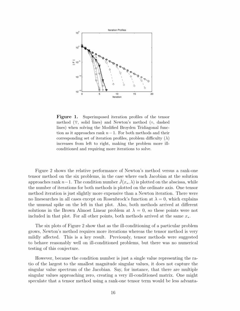
As a prelude to these results and to help explain what is happening in theseexperiments, we first provide a graphical description. Figure 1 shows the typicaliteration profiles for different values of λ that we observed. This figure graphs thefunction value at each iteration for the tensor and Newton methods on a typicalproblem approaching rank n − 1 with various values of λ = 0, 0.9, 0.99, 0.999, . . . , 1.All of the tensor method profiles are bunched together on the left, requiring fewiterations even as λ nears 1, whereas the profiles of Newton’s method are spread outand require increasingly more iterations for convergence as the problem becomes moreill-conditioned. This plot of iteration profiles is typical for all problems. Thus, whileall of the tensor runs display superlinear convergence throughout the iterations, it isevident that Newton’s method converges linearly for a number of iterations beforeaccelerating to quadratic convergence. With increasing ill-conditioning, the region ofquadratic convergence for Newton’s method shrinks in size, acting as if the problemwere singular outside of this region.

15

0 5 10 15 2010−15

10−10

10−5

100

105

Iteration

|| F

||

Iteration Profiles

Figure 1. Superimposed iteration profiles of the tensormethod (O, solid lines) and Newton’s method (, dashedlines) when solving the Modified Broyden Tridiagonal func-tion as it approaches rank n−1. For both methods and theircorresponding set of iteration profiles, problem difficulty (λ)increases from left to right, making the problem more ill-conditioned and requiring more iterations to solve.

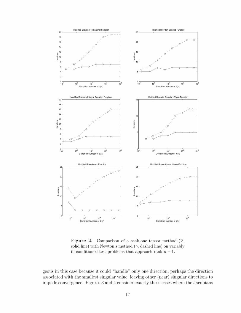
Figure 2 shows the relative performance of Newton’s method versus a rank-onetensor method on the six problems, in the case where each Jacobian at the solutionapproaches rank n−1. The condition number J(x∗, λ) is plotted on the abscissa, whilethe number of iterations for both methods is plotted on the ordinate axis. One tensormethod iteration is just slightly more expensive than a Newton iteration. There wereno linesearches in all cases except on Rosenbrock’s function at λ = 0, which explainsthe unusual spike on the left in that plot. Also, both methods arrived at differentsolutions in the Brown Almost Linear problem at λ = 0, so these points were notincluded in that plot. For all other points, both methods arrived at the same x∗.

The six plots of Figure 2 show that as the ill-conditioning of a particular problemgrows, Newton’s method requires more iterations whereas the tensor method is verymildly affected. This is a key result. Previously, tensor methods were suggestedto behave reasonably well on ill-conditioned problems, but there was no numericaltesting of this conjecture.

However, because the condition number is just a single value representing the ra-tio of the largest to the smallest magnitude singular values, it does not capture thesingular value spectrum of the Jacobian. Say, for instance, that there are multiplesingular values approaching zero, creating a very ill-conditioned matrix. One mightspeculate that a tensor method using a rank-one tensor term would be less advanta-

16

100 102 104 106 1080

2

4

6

8

10

12

14

16

18

20

Condition Number of J(x*)

Itera

tions

Modified Broyden Tridiagonal Function

100 102 104 106 1080

5

10

15

20

25


Itera

tions

Modified Broyden Banded Function

100 102 104 106 1080

2

4

6

8

10

12

14

16

18

20


Itera

tions

Modified Discrete Integral Equation Function

102 104 106 108 10100

5

10

15


Itera

tions

Modified Discrete Boundary Value Function

102 104 106 1080

5

10

15

20

25


Itera

tions

Modified Rosenbrock Function

102 104 1060

5

10

15

20

25


Itera

tions

Modified Brown Almost Linear Function

Figure 2. Comparison of a rank-one tensor method (O,solid line) with Newton’s method (, dashed line) on variablyill-conditioned test problems that approach rank n− 1.

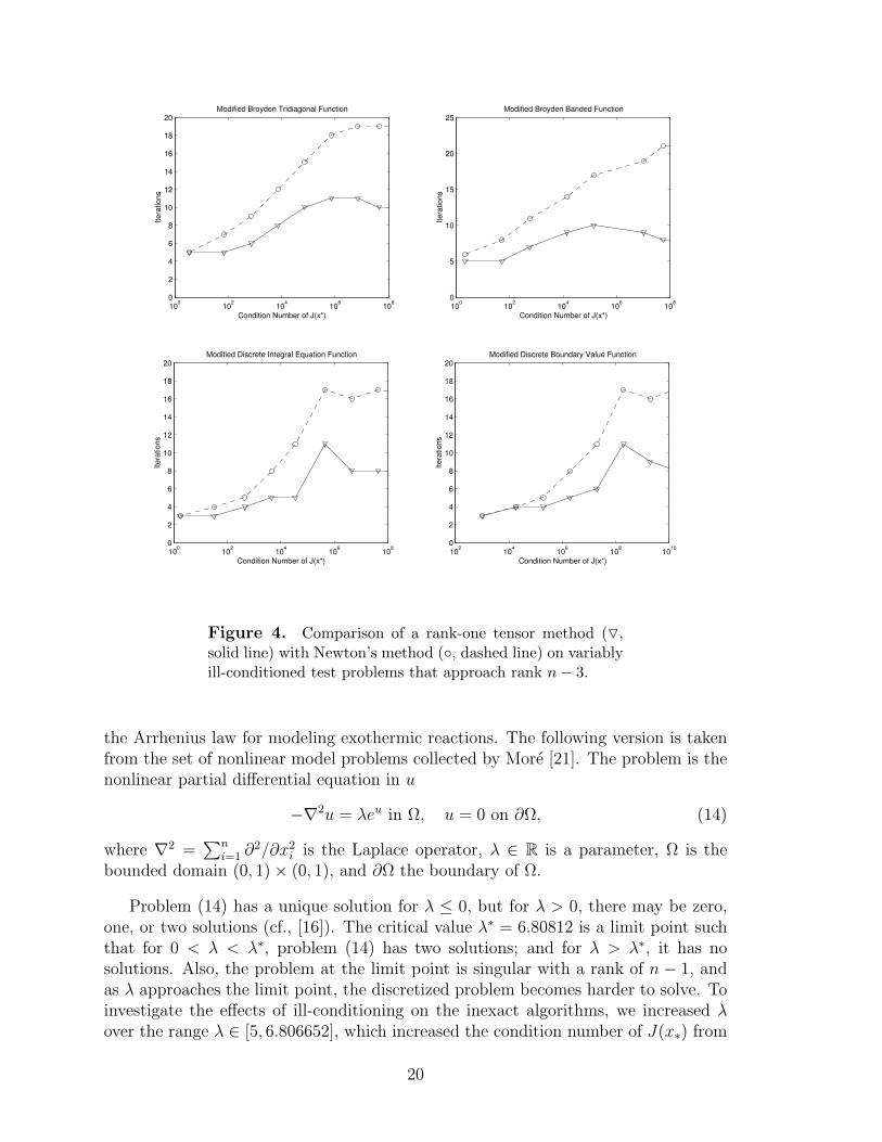
geous in this case because it could “handle” only one direction, perhaps the directionassociated with the smallest singular value, leaving other (near) singular directions toimpede convergence. Figures 3 and 4 consider exactly these cases where the Jacobians

17

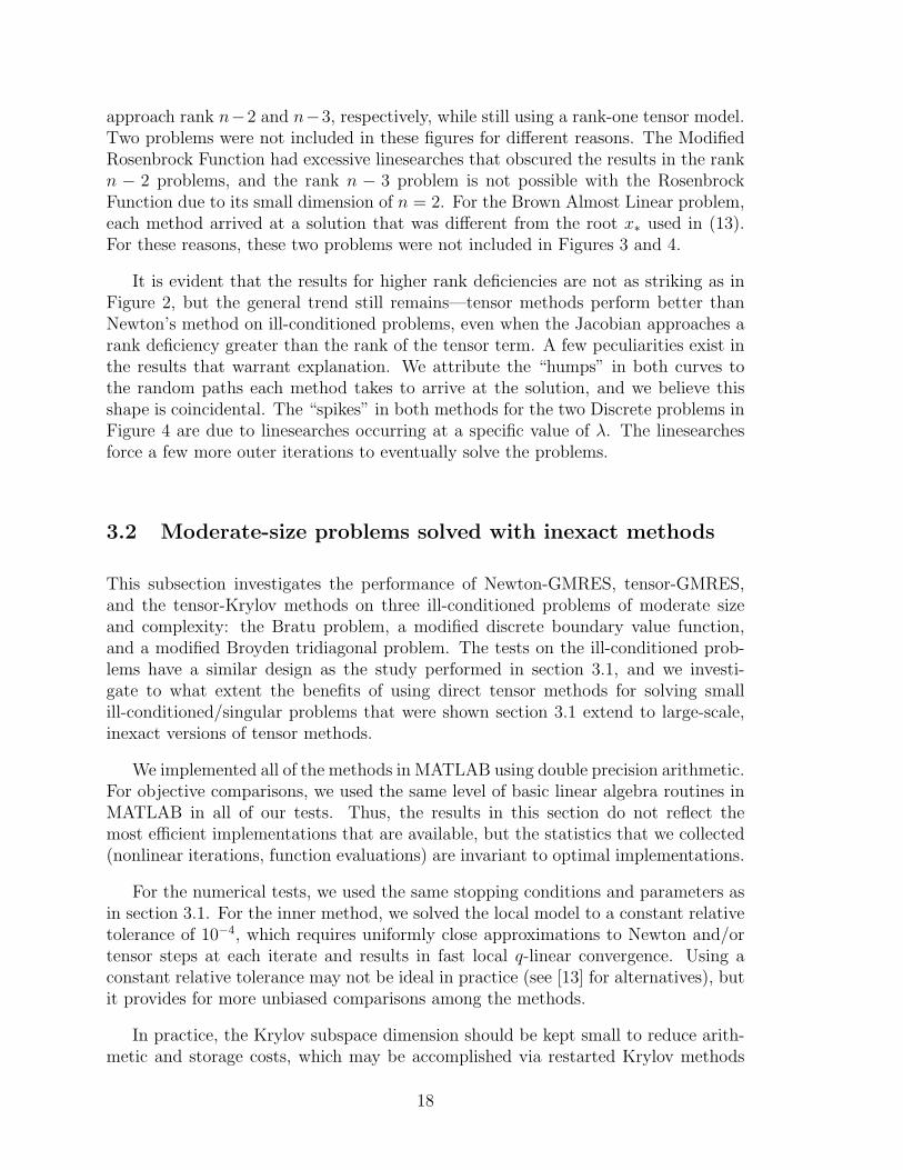
approach rank n−2 and n−3, respectively, while still using a rank-one tensor model.Two problems were not included in these figures for different reasons. The ModifiedRosenbrock Function had excessive linesearches that obscured the results in the rankn − 2 problems, and the rank n − 3 problem is not possible with the RosenbrockFunction due to its small dimension of n = 2. For the Brown Almost Linear problem,each method arrived at a solution that was different from the root x∗ used in (13).For these reasons, these two problems were not included in Figures 3 and 4.

It is evident that the results for higher rank deficiencies are not as striking as inFigure 2, but the general trend still remains—tensor methods perform better thanNewton’s method on ill-conditioned problems, even when the Jacobian approaches arank deficiency greater than the rank of the tensor term. A few peculiarities exist inthe results that warrant explanation. We attribute the “humps” in both curves tothe random paths each method takes to arrive at the solution, and we believe thisshape is coincidental. The “spikes” in both methods for the two Discrete problems inFigure 4 are due to linesearches occurring at a specific value of λ. The linesearchesforce a few more outer iterations to eventually solve the problems.

3.2 Moderate-size problems solved with inexact methods

This subsection investigates the performance of Newton-GMRES, tensor-GMRES,and the tensor-Krylov methods on three ill-conditioned problems of moderate sizeand complexity: the Bratu problem, a modified discrete boundary value function,and a modified Broyden tridiagonal problem. The tests on the ill-conditioned prob-lems have a similar design as the study performed in section 3.1, and we investi-gate to what extent the benefits of using direct tensor methods for solving smallill-conditioned/singular problems that were shown section 3.1 extend to large-scale,inexact versions of tensor methods.

We implemented all of the methods in MATLAB using double precision arithmetic.For objective comparisons, we used the same level of basic linear algebra routines inMATLAB in all of our tests. Thus, the results in this section do not reflect themost efficient implementations that are available, but the statistics that we collected(nonlinear iterations, function evaluations) are invariant to optimal implementations.

For the numerical tests, we used the same stopping conditions and parameters asin section 3.1. For the inner method, we solved the local model to a constant relativetolerance of 10−4, which requires uniformly close approximations to Newton and/ortensor steps at each iterate and results in fast local q-linear convergence. Using aconstant relative tolerance may not be ideal in practice (see [13] for alternatives), butit provides for more unbiased comparisons among the methods.

In practice, the Krylov subspace dimension should be kept small to reduce arith-metic and storage costs, which may be accomplished via restarted Krylov methods

18

100 102 104 106 1080

2

4

6

8

10

12

14

16

18

20


Itera

tions


100 102 104 106 1080

5

10

15

20

25


Itera

tions

Modified Broyden Banded Function

100 102 104 106 108 10100

2

4

6

8

10

12

14

16

18

20


Itera

tions


102 104 106 108 10100

2

4

6

8

10

12

14

16

18

20


Itera

tions



and preconditioning. However, to eliminate any ill effects of small Krylov subspacespreventing convergence in the local model and affecting the outer iterations, the max-imum Krylov subspace was set to the problem dimension, mmax = n, and the solverwas not restarted. We used preconditioners that are appropriate for the problem, andthey will be discussed with each problem.

In the next three subsections, we present numerical results on the ill-conditionedproblems. The results of the tensor-Krylov method TK2 are virtually identical toTK2+, so we do not include them here.

3.2.1 Bratu problem

The Bratu problem is a simplified model for nonlinear diffusion phenomena occurring,for example, in semiconductors and combustion, where the source term is related to

19

100 102 104 106 1080

2

4

6

8

10

12

14

16

18

20


Itera

tions


100 102 104 106 1080

5

10

15

20

25Modified Broyden Banded Function


Itera

tions

100 102 104 106 1080

2

4

6

8

10

12

14

16

18

20


Itera

tions


102 104 106 108 10100

2

4

6

8

10

12

14

16

18

20


Itera

tions



the Arrhenius law for modeling exothermic reactions. The following version is takenfrom the set of nonlinear model problems collected by More [21]. The problem is thenonlinear partial differential equation in u

−∇2u = λeu in Ω, u = 0 on ∂Ω, (14)

where ∇2 =∑n

i=1 ∂2/∂x2i is the Laplace operator, λ ∈ R is a parameter, Ω is the

bounded domain (0, 1)× (0, 1), and ∂Ω the boundary of Ω.

Problem (14) has a unique solution for λ ≤ 0, but for λ > 0, there may be zero,one, or two solutions (cf., [16]). The critical value λ∗ = 6.80812 is a limit point suchthat for 0 < λ < λ∗, problem (14) has two solutions; and for λ > λ∗, it has nosolutions. Also, the problem at the limit point is singular with a rank of n − 1, andas λ approaches the limit point, the discretized problem becomes harder to solve. Toinvestigate the effects of ill-conditioning on the inexact algorithms, we increased λover the range λ ∈ [5, 6.806652], which increased the condition number of J(x∗) from

20

about 103 to 106.

When testing the Bratu problem, the initial approximate solution was zero on auniform grid of size 31 × 31. The Laplace operator was discretized using centereddifferences (5-point stencil), and our preconditioner was also the centered differencesdiscretization of the Laplace operator. We computed Jacobian-vector products usingfirst-order forward differences. Hence, the number of function evaluations is the sumof the total number of Arnoldi iterations, the number of linesearch backtracks (ifany), and the total number of nonlinear iterations. Thus, the number of functionevaluations provides a relative measure of overall work for each algorithm.

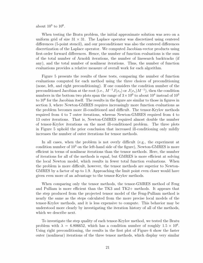
Figure 5 presents the results of these tests, comparing the number of functionevaluations computed for each method using the three choices of preconditioning(none, left, and right preconditioning). If one considers the condition number of thepreconditioned Jacobian at the root (i.e., M−1J(x∗) or J(x∗)M

−1), then the conditionnumbers in the bottom two plots span the range of 3×100 to about 104 instead of 103

to 106 for the Jacobian itself. The results in the figure are similar to those in figures insection 3, where Newton-GMRES requires increasingly more function evaluations asthe problem becomes more ill-conditioned and difficult. The tensor-Krylov methodsrequired from 4 to 7 outer iterations, whereas Newton-GMRES required from 4 to13 outer iterations. That is, Newton-GMRES required almost double the numberof tensor-Krylov iterations on the most ill-conditioned problem. The three plotsin Figure 5 uphold the prior conclusion that increased ill-conditioning only mildlyincreases the number of outer iterations for tensor methods.

In all cases, when the problem is not overly difficult (e.g., the experiment atcondition number of 103 on the left-hand side of the figure), Newton-GMRES is moreefficient in terms of nonlinear iterations than the tensor methods. Here, the numberof iterations for all of the methods is equal, but GMRES is more efficient at solvingthe local Newton model, which results in fewer total function evaluations. Whenthe problem is more difficult, however, the tensor methods are superior to Newton-GMRES by a factor of up to 1.9. Approaching the limit point even closer would havegiven even more of an advantage to the tensor-Krylov methods.

When comparing only the tensor methods, the tensor-GMRES method of Fengand Pulliam is more efficient than the TK3 and TK2+ methods. It appears thatthe step produced from the projected tensor model of the Feng-Pulliam method isnearly the same as the steps calculated from the more precise local models of thetensor-Krylov methods, and it is less expensive to compute. This behavior may beunderstood more clearly by investigating the iteration history of all of the methods,which we describe next.

To investigate the step quality of each tensor-Krylov method, we tested the Bratuproblem with λ = 6.806652, which has a condition number of roughly 1.5 × 106.Using right preconditioning, the results in the first plot of Figure 6 show the fasterouter (nonlinear) iterations of the three tensor methods, which display very similar

21

103

104

105

106

0

200

400

600

800

1000No Preconditioning

Fun

ctio

n E

valu

atio

ns

Newton−GMRESTensor−GMRESTK3TK2+

103

104

105

106

0

20

40

60

80

100Left Preconditioning

Fun

ctio

n E

valu

atio

ns

103

104

105

106

0

20

40

60

80

100Right Preconditioning


Fun

ctio

n E

valu

atio

ns

Figure 5. Effects of ill-conditioning on the inexact algo-rithms as seen in the Bratu problem.

performance. All methods start by exhibiting linear convergence until the respectivemethod can overcome the near singularity and accelerate convergence. The tensormethods accelerate convergence sooner than Newton-GMRES (iteration 2 versus it-eration 5), and this is typical behavior for ill-conditioned problems—Newton-typemethods branch into superlinear convergence later and later as the ill-conditioninggrows. Because the forcing term for the inner iterative method is constant (insteadof decreasing each iteration), all methods exhibit asymptotic linear convergence, asevidenced by their straight trajectories near the solution.

When we consider function evaluations in the bottom plot, the tensor-Krylovmethods separate from the Feng-Pulliam method. The block size of the method is aclear indicator of the relative efficiency of the method. Specifically, tensor-GMRES,which uses the scalar (block size one) implementation of GMRES, is more efficientthan TK2+ (block size two) and TK3 (block size three). The Bratu problem is uniqueamong our tests in that the steps computed from a projected local tensor model are ofroughly the same quality as the steps from TK2+ and TK3. Therefore, the number ofouter iterations are the same, but because tensor-GMRES is more efficient in solvingthe local model, tensor-GMRES has the advantage.

22

0 2 4 6 8 10 12 1410

−15

10−10

10−5

100

Outer Iterations||

F ||

0 10 20 30 40 50 60 70 8010

−15

10−10

10−5

100

Function Evaluations

|| F

||



Figure 6. Example iteration history on the Bratu problemat λ = 6.806652.

3.2.2 Modified discrete boundary value problem

The discrete boundary value problem is a simple test problem from [22]. The standarddiscrete boundary value problem is

fi(x) = 2xi − xi−1 − xi+1 + 12h2(xi + ti + 1)3, 1 ≤ i ≤ n, (15)

where h = 1n+1

, ti = ih, and x0 = xn+1 = 0. The initial approximate solution iszero on a problem size of n = 100 equations. For our tests, we have modified (15) inaccordance with equation (13) of section 3.1.

When testing this problem, we used a preconditioner that corresponds to theJacobian of (15) but without the term ti. We computed Jacobian-vector productsusing an analytic evaluation of the Jacobian, and we tallied the number of “functionevaluation equivalents,” which is the sum of function evaluations and Jacobian-vectorproducts. If these products were approximated by first-order forward differences, asis generally the case with complex problems, then “function evaluation equivalents”would be equal to the number of function evaluations. This number also provides arelative measure of overall work for each algorithm.

23

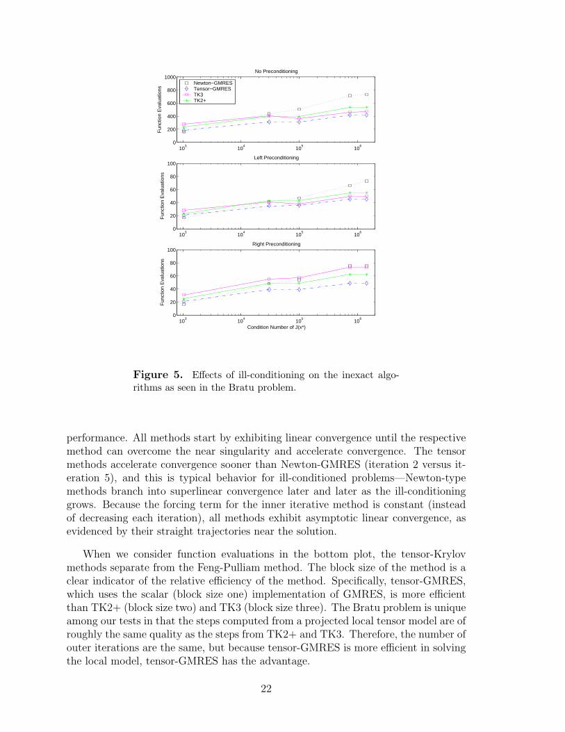
Figure 7 presents the results of these tests, comparing the number of functionevaluation equivalents computed for each method using the three choices of pre-conditioning (none, left, and right preconditioning) for the various values of λ =1 − 10−j, j = 0, 1, 2, . . . in equation (13). If one considers the condition number ofthe preconditioned Jacobian at the root (i.e., M−1J(x∗) or J(x∗)M

−1), then the con-dition numbers in the bottom two plots span the range of 1 × 100 to about 2 × 106

(left preconditioning) or 2× 108 (right preconditioning) instead of 4× 103 to 2× 109

for the Jacobian, not counting the singular case.

The results for the modified discrete boundary value problem are similar to thoseof the Bratu problem in Figure 5: Newton-GMRES requires increasingly more func-tion evaluations as the problem becomes more ill-conditioned, whereas the number offunction evaluations required by the tensor methods increases to a lesser extent. Itis interesting to note that the tensor methods are virtually identical in performancewithout preconditioning and resemble the results in section 3.1. However, once pre-conditioning is used, the tensor methods are affected by the ill-conditioning of theproblem, yet still to a lesser extent than Newton-GMRES.

103

104

105

106

107

108

109

0

500

1000


Fun

ctio

n E

valu

atio

ns E

quiv

alen

ts


103

104

105

106

107

108

109

0

20

40

60


Fun

ctio

n E

valu

atio

n E

quiv

alen

ts

103

104

105

106

107

108

109

0

20

40

60



Fun

ctio

n E

valu

atio

n E

quiv

alen

ts

Figure 7. Effects of ill-conditioning on the inexact algo-rithms as seen in the discrete boundary value problem.

When comparing only the tensor methods while using left and right precondition-

24

ing, the tensor-GMRES method of Feng and Pulliam is more efficient than the TK3and TK2+ methods on the easier problems but less efficient on the hardest problems,which is different from the experience with the Bratu problem above. We explain thisrelative difference by noting that Tensor-GMRES required more nonlinear iterationsas the problem grew more ill-conditioned. Because the tensor-Krylov methods gen-erally require more Arnoldi (inner) iterations to solve the local tensor model due tothe less efficient block-Arnoldi process, any computational savings must come fromfewer nonlinear (outer) iterations.

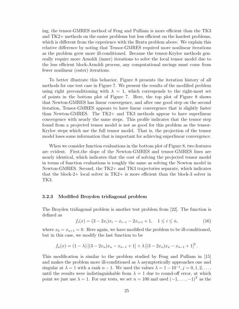
To better illustrate this behavior, Figure 8 presents the iteration history of allmethods for one test case in Figure 7. We present the results of the modified problemusing right preconditioning with λ = 1, which corresponds to the right-most setof points in the bottom plot of Figure 7. Here, the top plot of Figure 8 showsthat Newton-GMRES has linear convergence, and after one good step on the seconditeration, Tensor-GMRES appears to have linear convergence that is slightly fasterthan Newton-GMRES. The TK2+ and TK3 methods appear to have superlinearconvergence with nearly the same steps. This profile indicates that the tensor stepfound from a projected tensor model is not as good for this problem as the tensor-Krylov steps which use the full tensor model. That is, the projection of the tensormodel loses some information that is important for achieving superlinear convergence.

When we consider function evaluations in the bottom plot of Figure 8, two featuresare evident. First,the slope of the Newton-GMRES and tensor-GMRES lines arenearly identical, which indicates that the cost of solving the projected tensor modelin terms of function evaluations is roughly the same as solving the Newton model inNewton-GMRES. Second, the TK2+ and TK3 trajectories separate, which indicatesthat the block-2+ local solver in TK2+ is more efficient than the block-3 solver inTK3.

3.2.3 Modified Broyden tridiagonal problem

The Broyden tridiagonal problem is another test problem from [22]. The function isdefined as

fi(x) = (3− 2xi)xi − xi−1 − 2xi+1 + 1, 1 ≤ i ≤ n, (16)

where x0 = xn+1 = 0. Here again, we have modified the problem to be ill-conditioned,but in this case, we modify the last function to be

fn(x) = (1− λ) [(3− 2xn)xn − xn−1 + 1] + λ [(3− 2xn)xn − xn−1 + 1]2 .

This modification is similar to the problem studied by Feng and Pulliam in [15]and makes the problem more ill-conditioned as λ asymptotically approaches one andsingular at λ = 1 with a rank n− 1. We used the values λ = 1− 10−j, j = 0, 1, 2, . . . ,until the results were indistinguishable from λ = 1 due to round-off error, at whichpoint we just use λ = 1. For our tests, we set n = 100 and used (−1, . . . ,−1)T as the

25

0 2 4 6 8 10 1210

−15

10−10

10−5

100

Outer Iterations

|| F

||

0 10 20 30 40 50 60 70 8010

−15

10−10

10−5

100

Function Evaluation Equivalents

|| F

||



Figure 8. Example iteration history on the discrete bound-ary value problem at λ = 1.

starting vector. We used the Jacobian of (16) as our preconditioner for all values ofλ.

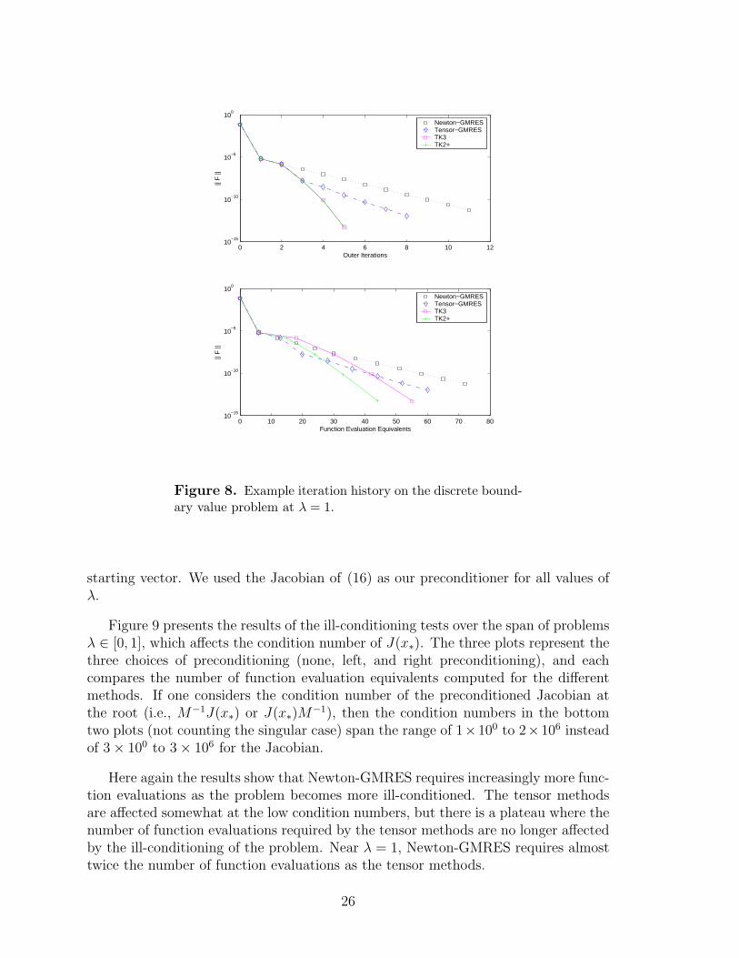
Figure 9 presents the results of the ill-conditioning tests over the span of problemsλ ∈ [0, 1], which affects the condition number of J(x∗). The three plots represent thethree choices of preconditioning (none, left, and right preconditioning), and eachcompares the number of function evaluation equivalents computed for the differentmethods. If one considers the condition number of the preconditioned Jacobian atthe root (i.e., M−1J(x∗) or J(x∗)M

−1), then the condition numbers in the bottomtwo plots (not counting the singular case) span the range of 1×100 to 2×106 insteadof 3× 100 to 3× 106 for the Jacobian.

Here again the results show that Newton-GMRES requires increasingly more func-tion evaluations as the problem becomes more ill-conditioned. The tensor methodsare affected somewhat at the low condition numbers, but there is a plateau where thenumber of function evaluations required by the tensor methods are no longer affectedby the ill-conditioning of the problem. Near λ = 1, Newton-GMRES requires almosttwice the number of function evaluations as the tensor methods.

26

100

101

102

103

104

105

106

107

0

100

200

300


Fun

ctio

n E

valu

atio

n E

quiv

alen

ts


100

101

102

103

104

105

106

107

0

10

20

30

40

50

60


Fun

ctio

n E

valu

atio

n E

quiv

alen

ts

100

101

102

103

104

105

106

107

0

10

20

30

40

50

60



Fun

ctio

n E

valu

atio

n E

quiv

alen

ts

Figure 9. Effects of ill-conditioning on the inexact algo-rithms as seen in the modified Broyden Tridiagonal problem.

When comparing only the tensor methods while using left and right precondition-ing, the tensor-GMRES method of Feng and Pulliam is roughly comparable to TK3.The TK2+ method is more efficient on all problems except one, where tensor-GMRESis the best. In comparison with Newton-GMRES on the easier problems with left orright preconditioning, TK2+ requires the same number or fewer function evaluationequivalents.

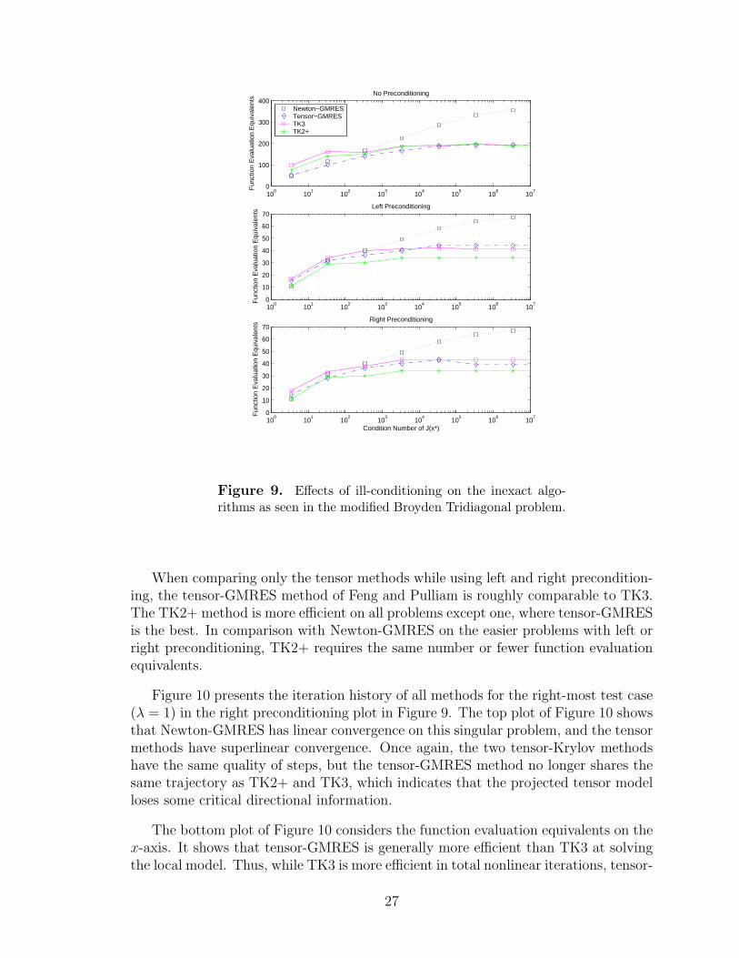
Figure 10 presents the iteration history of all methods for the right-most test case(λ = 1) in the right preconditioning plot in Figure 9. The top plot of Figure 10 showsthat Newton-GMRES has linear convergence on this singular problem, and the tensormethods have superlinear convergence. Once again, the two tensor-Krylov methodshave the same quality of steps, but the tensor-GMRES method no longer shares thesame trajectory as TK2+ and TK3, which indicates that the projected tensor modelloses some critical directional information.

The bottom plot of Figure 10 considers the function evaluation equivalents on thex-axis. It shows that tensor-GMRES is generally more efficient than TK3 at solvingthe local model. Thus, while TK3 is more efficient in total nonlinear iterations, tensor-

27

0 5 10 15 20 2510

−15

10−10

10−5

100

105

Outer Iterations

|| F

||

0 10 20 30 40 50 60 7010

−15

10−10

10−5

100

105

Function Evaluation Equivalents

|| F

||



Figure 10. Example iteration history on the modified Broy-den tridiagonal problem at λ = 1.

GMRES is more efficient at solving the local model, which accounts for the difference.Another feature evident in the bottom plot is that the TK2+ and TK3 trajectoriesseparate. As with the discrete boundary value problem above, this indicates that theblock-2+ local solver in TK2+ is more efficient than the block-3 solver in TK3.

4 Summary and conclusions

This paper has investigated the performance of small- and large-scale tensor methodson problems over a range of conditionings, from well-conditioned to ill-conditionedto singular. Our results showed that tensor methods outperform Newton’s methodas the problems become more ill-conditioned. Prior to this investigation, studies ondirect tensor methods only focused on singular problems or on general problems thatare well-conditioned.

Specifically, our results show that, eventual quadratic convergence notwithstand-ing, the performance of Newton’s method will degrade as the ill-conditioning grows,

28

whereas tensor methods appear to be relatively unaffected or only mildly affected(in the case of larger rank deficiencies). Newton-based methods do not handle thesesingular problems well because they converge linearly to the solution and, in somecases, with poor accuracy.

For the large-scale methods, despite the use of an iterative inner method with anapproximate solve, the tensor-Krylov methods appear to retain superlinear conver-gence properties on ill-conditioned problems. On the other hand, Newton-GMRES isaffected by the ill-conditioning and branches into superlinear convergence later andlater as the problems become more ill-conditioned. Thus, tensor methods are espe-cially useful for large-scale problems that are highly ill-conditioned or singular, whereNewton-based algorithms exhibit very slow convergence.

There are many important and practical problems that have ill-conditioned orsingular Jacobian matrices at the solution, such as large PDE problems that ex-hibit “turning points” and/or shocks. The conclusions of this research indicate thatconcepts from tensor methods may benefit algorithms for bifurcation tracking andstability analysis. We intend to investigate these applications in future research.

29

References

[1] Brett W. Bader. Tensor-Krylov methods for solving large-scale systems of non-linear equations. SIAM J. Numer. Anal. submitted.

[2] Brett W. Bader. Tensor-Krylov methods for solving large-scale systems of non-linear equations. PhD thesis, University of Colorado, Boulder, Department ofComputer Science, 2003.

[3] Ali Bouaricha. Solving large sparse systems of nonlinear equations and nonlinearleast squares problems using tensor methods on sequential and parallel computers.PhD thesis, University of Colorado, Boulder, Department of Computer Science,1992.

[4] Peter N. Brown and Alan C. Hindmarsh. Reduced storage methods in stiff ODEsystems. J. Appl. Math. Comput., 31:40–91, 1989.

[5] Peter N. Brown and Yousef Saad. Hybrid Krylov methods for nonlinear systemsof equations. SIAM J. Sci. Statist. Comput., 11:450–481, 1990.

[6] Peter N. Brown and Yousef Saad. Convergence theory of nonlinear Newton-Krylov algorithms. SIAM J. Optim., 4:297–330, 1994.

[7] T. F. Chan and K. R. Jackson. The use of iterative linear equation solvers incodes for large systems of stiff IVPs for ODEs. SIAM J. Sci. Statist. Comput.,7:378–417, 1986.

[8] D. W. Decker, H. B. Keller, and C. T. Kelley. Convergence rate for Newton’smethod at singular points. SIAM J. Numer. Anal., 20:296–314, 1983.

[9] D. W. Decker and C. T. Kelley. Newton’s method at singular points I. SIAM J.Numer. Anal., 17:66–70, 1980.

[10] D. W. Decker and C. T. Kelley. Newton’s method at singular points II. SIAMJ. Numer. Anal., 17:465–471, 1980.

[11] D. W. Decker and C. T. Kelley. Convergence acceleration for Newton’s methodat singular points. SIAM J. Numer. Anal., 19:219–229, 1982.

[12] J. E. Dennis, Jr. and Robert B. Schnabel. Numerical Methods for UnconstrainedOptimization and Nonlinear Equations. Prentice-Hall, Englewood Cliffs, NJ,1983.

[13] Stanley C. Eisenstat and Homer F. Walker. Choosing the forcing terms in aninexact Newton method. SIAM J. Sci. Comput., 17:16–32, 1996.

[14] Dan Feng, Paul D. Frank, and Robert B. Schnabel. Local convergence analysis oftensor methods for nonlinear equations. Math. Programming, 62:427–459, 1993.

30

[15] Dan Feng and Thomas H. Pulliam. Tensor-GMRES method for large systems ofnonlinear equations. SIAM J. Optim., 7:757–779, 1997.

[16] R. Glowinski, H. B. Keller, and L. Reinhart. Continuation-conjugate gradientmethods for the least squares solution of nonlinear boundary value problems.SIAM J. Sci. Statist. Comput., 6:793–832, 1985.

[17] A. Griewank. On solving nonlinear equations with simple singularities or nearlysingular solutions. SIAM Review, 27:537–563, 1985.

[18] A. Griewank and M. R. Osborne. Analysis of Newton’s method at irregularsingularities. SIAM J. Numer. Anal., 20:747–773, 1983.

[19] C. T. Kelley. Iterative methods for linear and nonlinear equations. Society forIndustrial and Applied Mathematics, Philadelphia, 1995.

[20] C. T. Kelley and R. Suresh. A new acceleration method for Newton’s methodat singular points. SIAM J. Numer. Anal., 20:1001–1009, 1983.

[21] Jorge J. More. A collection of nonlinear model problems. Lectures Appl. Math.,26:723–762, 1990.

[22] Jorge J. More, Burton S. Garbow, and Kenneth E. Hillstrom. Testing uncon-strained optimization software. ACM Trans. Math. Software, 7:17–41, 1981.

[23] Jorge Nocedal and S. J. Wright. Numerical Optimization. Springer-Verlag, NewYork, 1999.

[24] G. W. Reddien. On Newton’s method for singular problems. SIAM J. Numer.Anal., 15:993–996, 1978.

[25] Yousef Saad. Analysis of augmented Krylov subspace methods. SIAM J. MatrixAnal. Appl., 18:435–449, 1997.

[26] Robert B. Schnabel and Paul D. Frank. Tensor methods for nonlinear equations.SIAM J. Numer. Anal., 21:815–843, 1984.

31

DISTRIBUTION:

5 MS 0316 Brett W. Bader, 9233

2 MS 9018 Central Technical Files, 8945-1

1 MS 0899 Technical Library, 9616

32

Documents

On the Performance of Tensor Methods for Solving Ill ... the Performance of Tensor Methods for Solving Ill-conditioned Problems Brett W. Bader and Robert B. Schnabel ... at the solution.Published