Embed Size (px)
Citation preview
THESIS FOR THE DEGREE OF LICENTIATE OF ENGINEERING
On the Optimization of Schedules of aMultitask Production Cell
Karin Thörnblad
Volvo Aero CorporationDepartment of Logistics Development
SE-461 81 Trollhättan, Sweden
and
Department of Mathematical Sciences, Chalmers University of TechnologyDepartment of Mathematical Sciences, University of Gothenburg
SE-412 96 Göteborg, Sweden
Göteborg, 2011
This work was supported by:Volvo Aero, Vetenskapsrådet (The Swedish Research Council), and NFFP (NationalAviation Engineering Research Programme).
Cover illustration: An example of an optimal schedule for the resources in the mul-titask production cell; see Figure 9 in the thesis.
On the Optimization of Schedules of a Multitask Production CellKarin Thörnblad
c©Karin Thörnblad, 2011
NO 2011:19ISSN 1652-9715Department of Mathematical Sciences, Chalmers University of TechnologyDepartment of Mathematical Sciences, University of GothenburgSE-412 96 GöteborgSwedenTelephone +46 (0)31 772 1000
Printed in Göteborg, Sweden 2011
On the Optimization of Schedules of aMultitask Production Cell
Karin Thörnblad
Department of Logistics Development, Volvo Aero Corporation
and
Department of Mathematical Sciences, Chalmers University of TechnologyDepartment of Mathematical Sciences, University of Gothenburg
Abstract
Volvo Aero has invested in a complex production cell containing a set of multi-purpose machines. The problem of finding optimal schedules for this multitask cellis a complex combinatorial optimization problem which is recognized as a flexiblejob shop problem.
This thesis proposes an approach to find such schedules using mathematical op-timization. The mathematical models developed so far are presented together witha study of their interrelations, both from a computational and from a modelling per-spective. One result of the study is that one of these models, a time-indexed modelwith nail variables, outperforms all the others presented. To our knowledge, thismodel is the first for the flexible job shop problem using this type of variables.
In order to reduce the number of variables in the time-indexed models, a heuris-tic has been developed which finds an upper bound on the optimal value of themakespan.
Computational results are presented for several variants of the time-indexed mod-el and the engineer’s model, the latter belonging to a family of models widely usedin job shop scheduling. The objective employed for the computations is the mini-mization of a weighted sum of the total tardiness and the sum of job completiontimes.
A comparison is made between optimal schedules emanating from the time-indexed model and schedules resulting from the use of three well-known dispatch-ing rules, using the data from 21 real production scenarios. The tardiness and thesum of job completion times are on average 6–22% larger in the schedules result-ing from the use of the dispatching rules compared to those obtained in the optimalschedules. The first appended paper provides the results from a similar comparisonfor a number of scenarios, constructed by using data emanating from the multitaskcell.
The computational complexity of the problem of scheduling the multitask cell isalso investigated. The second appended paper contains a proof of a complexity resultfor a related scheduling problem, namely flow-shop scheduling with deterioratingjobs.
iii

This thesis has been written in close cooperation with the Department of LogisticsDevelopment at Volvo Aero Corporation.
Keywords: mathematical optimization; flexible job shop scheduling; mixed integerlinear programming (MILP); complexity analysis; mathematical modelling; produc-tion planning; multi-purpose machine; dispatching rule; priority function; total flowtime; total tardiness; release date; due date
iv

Appended papers:
Paper I: Optimization of schedules for a multitask production cell, Proceedings of 22nd
Nofoma conference, Kolding, Denmark, 2010 (with Ann-Brith Strömberg, TorgnyAlmgren, and Michael Patriksson).
Paper II: A note on the complexity of flow-shop scheduling with deteriorating jobs, Pub-lished in Discrete Applied Mathematics, 159 (2011), pp. 251–253 (with Michael Pat-riksson).
Other publications, not included in this thesis:
A comparison of schedules resulting from priority rules and mathematical optimization fora real production cell, Proceedings of PLANs forsknings- och tillämpningskonferens,Skövde, Sweden, 2010 (with Linea Kjellsdotter Ivert).
Mathematical modelling of a real flexible job shop in aero engine component manufacturing,Proceedings of 10th Workshop on Models and Algorithms for Planning and Schedul-ing Problems, Nymburk, Czech Republic, 2011 (with Michael Patriksson, Ann-BrithStrömberg, and Torgny Almgren).
Optimering av scheman för en verklig produktionscell: tidsdiskretisering reducerar lösningsti-den utan att lösningarnas kvalitet försämras, Proceedings of PLANs forsknings- ochtillämpningskonferens, Norrköping, Sweden, 2011 (with Torgny Almgren, Ann-BrithStrömberg, and Michael Patriksson).
v

Acknowledgements
First of all, I would like to express my gratitude towards my industrial supervisorTorgny Almgren for taking the initiative to this project and for his constant supportand encouragement. I have been fortunate to have two nice academic supervisorsMichael Patriksson and Ann-Brith Strömberg. I thank both of you for always takingthe time for discussions and providing advice and for your wise guidance in thisinteresting subject.
I would also like to thank my colleagues at the department of Logistics Devel-opment at Volvo Aero (Fredrik, Sture, Ulla, Maria, and Joakim to name but a few)for your support and willingness to share experience, and for creating a good work-ing environment. I would like to thank the personnel working with the multitaskcell (especially Nicklas Gödebu, Christina Kann, and Martin Lundstedt) as well asthe project leader of the former multitask project, Fredrik Johansson, for your use-ful information and for putting up with all my questions. I would further like tothank Tomas Lindsta, manager of the production of high volume products, for yourencouraging support as a member of the steering committee.
A special thanks goes to Thomas Ericsson at the Department of Mathematical Sci-ences at Chalmers for your support with problems encountered during the compu-tational testing, and all the members of the optimization group and especially AdamWojciechowski for interesting discussions. Yet another special thanks to Linea Kjells-dotter Ivert at the Department of Technology Management and Economics (Divisionof Logistics and Transportation) at Chalmers for nice collaboration and for being agood friend.
Furthermore, I would like to gratefully acknowledge the financial support fromVolvo Aero, Vetenskapsrådet (The Swedish Research Council), and NFFP (NationalAviation Engineering Research Programme).
Finally, I would like to express my thanks to my family. My parents and parents-in-law for your constant support, Gabriel, for being an excellent IT consultant as wellas a wonderful supportive husband, and my three boys for bringing happiness andlaughter.
Karin ThörnbladTrollhättan, August 2011
vii

Contents
1 Introduction 11.1 Background . . . . . . . . . . . . . . . . . . . . . . . . . . . . . . . . . . 11.2 Aims and objectives . . . . . . . . . . . . . . . . . . . . . . . . . . . . . . 11.3 Limitations . . . . . . . . . . . . . . . . . . . . . . . . . . . . . . . . . . . 11.4 Outline . . . . . . . . . . . . . . . . . . . . . . . . . . . . . . . . . . . . . 2
2 The planning situation at Volvo Aero 22.1 The company Volvo Aero . . . . . . . . . . . . . . . . . . . . . . . . . . 22.2 The products . . . . . . . . . . . . . . . . . . . . . . . . . . . . . . . . . . 32.3 The multitask cell . . . . . . . . . . . . . . . . . . . . . . . . . . . . . . . 32.4 The production planning of the multitask cell . . . . . . . . . . . . . . . 5
3 Job shop scheduling: A subject orientation 63.1 The perspective of operations research . . . . . . . . . . . . . . . . . . . 6
3.1.1 Mathematical optimization . . . . . . . . . . . . . . . . . . . . . 63.1.2 Metaheuristics . . . . . . . . . . . . . . . . . . . . . . . . . . . . 8
3.2 The perspective of logistics . . . . . . . . . . . . . . . . . . . . . . . . . 9
4 On the complexity of scheduling problems 104.1 On the complexity of flow shop problems with deteriorating jobs . . . 114.2 On the complexity of flexible job shop problems . . . . . . . . . . . . . 114.3 Weak and strong formulations . . . . . . . . . . . . . . . . . . . . . . . . 12
5 Mathematical modelling 135.1 Definitions required for the MILP models . . . . . . . . . . . . . . . . . 13
5.1.1 Assumptions made for the mathematical formulations . . . . . 145.1.2 Indices and definitions of sets . . . . . . . . . . . . . . . . . . . . 145.1.3 Definition of parameters and time variables . . . . . . . . . . . 155.1.4 Realistic release dates and interoperation times . . . . . . . . . 175.1.5 Objectives for the scheduling of the multitask cell . . . . . . . . 19
5.2 The full engineer’s model . . . . . . . . . . . . . . . . . . . . . . . . . . 205.2.1 Definition of variables . . . . . . . . . . . . . . . . . . . . . . . . 205.2.2 The engineer’s mathematical optimization model . . . . . . . . 205.2.3 Preliminary computations using the full engineer’s model . . . 21
5.3 The machining/feasibility problem decomposition . . . . . . . . . . . . 225.3.1 The engineer’s model of the machining problem . . . . . . . . . 225.3.2 The feasibility problem . . . . . . . . . . . . . . . . . . . . . . . . 24
5.4 Time-indexed formulations . . . . . . . . . . . . . . . . . . . . . . . . . 265.4.1 Time intervals . . . . . . . . . . . . . . . . . . . . . . . . . . . . . 265.4.2 Definition of variables . . . . . . . . . . . . . . . . . . . . . . . . 275.4.3 New values for all time parameters . . . . . . . . . . . . . . . . 285.4.4 A time-indexed model with nail variables . . . . . . . . . . . . . 285.4.5 A time-indexed model with plateau variables . . . . . . . . . . 30
ix
5.4.6 Minimizing work load variance . . . . . . . . . . . . . . . . . . . 325.4.7 A heuristic for determining the time horizon . . . . . . . . . . . 34
6 Computational tests and results 366.1 Test data . . . . . . . . . . . . . . . . . . . . . . . . . . . . . . . . . . . . 376.2 Validation and tests . . . . . . . . . . . . . . . . . . . . . . . . . . . . . . 38
6.2.1 Estimated error due to the choice of ` for the time-indexedmodels . . . . . . . . . . . . . . . . . . . . . . . . . . . . . . . . . 38
6.2.2 Comparison of computation times for the different models . . . 406.2.3 Comparison with dispatching rules . . . . . . . . . . . . . . . . 426.2.4 The value of the parameter M for the engineer’s model . . . . . 44
7 Conclusions 47
8 Future research 48
9 Summary of appended papers 499.1 Paper I — Optimization of schedules for a multitask production cell . 499.2 Paper II — A note on the complexity of flow-shop scheduling with
deteriorating jobs . . . . . . . . . . . . . . . . . . . . . . . . . . . . . . . 49
x

1
1 Introduction
1.1 Background
Volvo Aero has invested in a complex production cell containing a set of multi-purpose machines, with the aim to decrease product costs, shorten lead times, andincrease the quality level and delivery precision. The planning and control of this so-called multitask cell result in a complex combinatorial optimization problem, whichneeds to be solved in a reasonable amount of time. The control system of the multi-task cell contains a built-in scheduling algorithm, which is based on a simple priorityfunction. In the master’s thesis [28], it was shown that this algorithm is not suffi-ciently efficient, as it is not adapted to the production of complex structures suchas the aircraft engine components, which is the case at Volvo Aero. Therefore, thebuilt-in scheduling algorithm is not in use and the production of components in themultitask cell is manually planned at present. This inferiority of the existing decisionsupport leads to unnecessarily long lead times and an inefficient use of the resources.
1.2 Aims and objectives
The overall aim of the research project is to contribute to the goal of enabling the con-struction of optimal, or near-optimal, schedules for multi-purpose production cells,similar to the Volvo Aero multitask cell. An algorithm which is fast and appropriatethen needs to be developed for the problem of scheduling the multitask cell, sincethe conditions are unceasingly changing with new jobs continuously arriving at thequeue.
This thesis focuses primarily on finding a mathematical optimization model thatcan be used for solving the problem of scheduling the processes in the multitask cellin a reasonable computation time. This goal is achieved by
• the development of a number of mixed integer linear programming (MILP)models for the scheduling problem at hand;
• the study of these models’ interrelations, from both a computational and amodelling perspective;
• a discussion on appropriate objective functions and their impact on the logisticperformance of the production cell.
1.3 Limitations
This thesis is limited to the study of the scheduling of the machine resources in themultitask cell. The number of staff in operation in the multitask cell is assumed to besufficient for performing the manual work associated with all the operations sched-uled, and their scheduling is therefore not included in the MILP models. Other areasnot taken into account in this thesis are the maintenance planning of the multitaskcell, and the availability of machining tools. All of these areas are subjects for futureresearch.
2 2 THE PLANNING SITUATION AT VOLVO AERO
1.4 Outline
In this thesis, we present all the MILP models of the scheduling problem that havebeen developed so far, together with computational results. Section 2.1 gives anoverview of the planning situation at Volvo Aero, where the supply chain, the prod-ucts, and the multitask cell are described.
In Section 3, a literature overview of possible approaches to problems similarto the problem of scheduling the multitask cell is given. First, the perspective ofoperations research is presented; both exact approaches—as mathematical optimiza-tion—and approximate approaches—as the use of metaheuristics—are described. Thesection ends with a description of the perspective of logistics. This is then followedby Section 4, dealing with the complexity of scheduling problems. First, a motivationfor the proof presented in [53] (Paper II) is given. The problem studied in Paper II isa so-called flow shop scheduling problem with deteriorating jobs.
The main section in this thesis is Section 5, where the MILP models for the prob-lem of scheduling the multitask cell are presented. A discussion regarding differ-ent objective functions is included. This section ends with a description of a greedyheuristic, developed with the aim of obtaining good feasible schedules. The heuris-tic also provides parameter values for use in the MILP models to ensure reducedcomputation times.
Computational results are presented in Section 6. It is clear that a time-indexedmodel with so-called nail variables outperforms all the other models developed sofar. To our knowledge, this model is the first model for the flexible job shop problemwhich uses this type of variables. Since the time-indexed model performs best, it isused in most of the computational tests performed. The consequences of the length ofthe discretization interval for the time-indexed model is investigated, and the modelis compared with the so-called engineer’s model, being of a common type used for theformulation of similar scheduling problems. A comparison between optimal sched-ules emanating from the time-indexed model and the schedules resulting from theuse of three well-known dispatching rules is also given. The impact of the choice ofa parameter for the engineer’s model on the computation times is presented as thelast test in this section. All data used for the tests described in Section 6 consist ofreal production scenarios from the multitask cell at Volvo Aero.
In Sections 7 and 8, conclusions and proposed areas for future research are found,and Section 9 contains a summary of the appended papers.
2 The planning situation at Volvo Aero
2.1 The company Volvo Aero
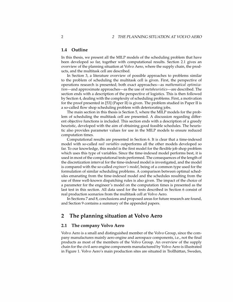
Volvo Aero is a small and distinguished member of the Volvo Group, since the com-pany manufactures mainly aero engine and aerospace components, i.e., not the finalproducts as most of the members of the Volvo Group. An overview of the supplychain for the civil aero engine components manufactured by Volvo Aero is illustratedin Figure 1. Volvo Aero’s main production sites are situated in Trollhättan, Sweden,
2.2 The products 3
in Kongsberg, Norway, and in Newington, Connecticut, USA. Since the main pro-duction is in the aero engine industry, the quality requirements are high. Therefore,the processing machines in the production are often very large and expensive, whilethe product volumes are small.
Figure 1: An overview of the supply chain for the civil aero engine components pro-duced by Volvo Aero.
The planning and control of the supply chain is affected by the fact that the pro-duction of aero engine components are subject to flight safety regulations issued byflight safety authorities. As an example, all suppliers have to be approved by the au-thorities, and Volvo Aero has to keep track of which mine the raw material for eachfinal product comes from. The operations performed by Volvo Aero also has to beapproved for each processing machine.
2.2 The products
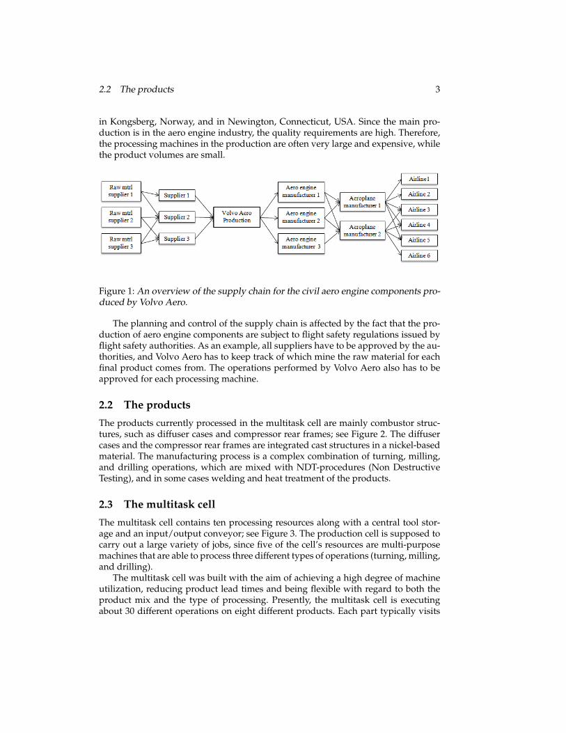
The products currently processed in the multitask cell are mainly combustor struc-tures, such as diffuser cases and compressor rear frames; see Figure 2. The diffusercases and the compressor rear frames are integrated cast structures in a nickel-basedmaterial. The manufacturing process is a complex combination of turning, milling,and drilling operations, which are mixed with NDT-procedures (Non DestructiveTesting), and in some cases welding and heat treatment of the products.
2.3 The multitask cell
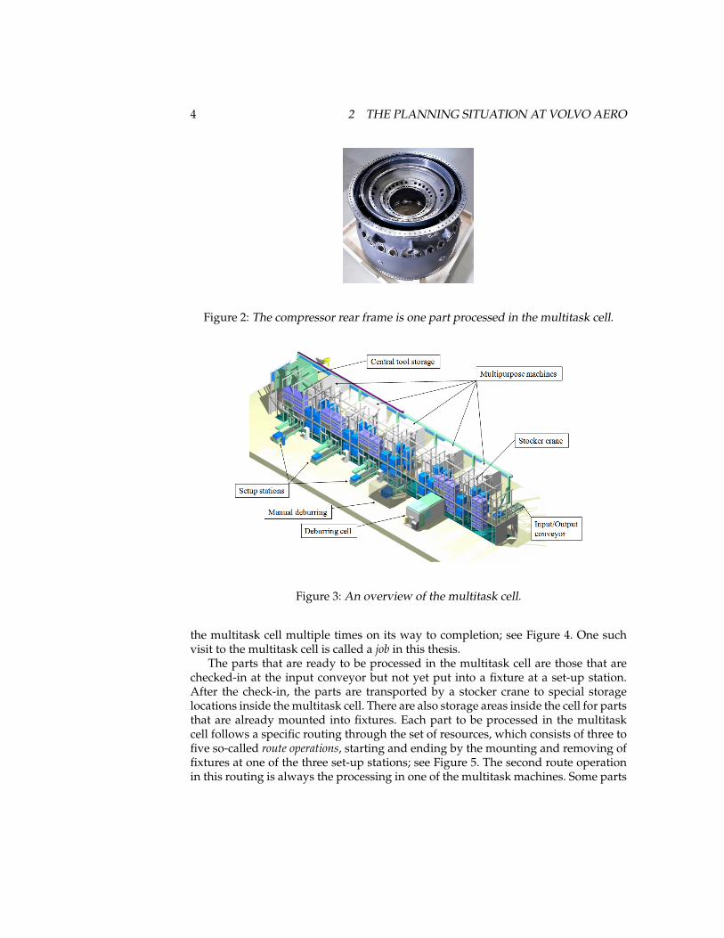
The multitask cell contains ten processing resources along with a central tool stor-age and an input/output conveyor; see Figure 3. The production cell is supposed tocarry out a large variety of jobs, since five of the cell’s resources are multi-purposemachines that are able to process three different types of operations (turning, milling,and drilling).
The multitask cell was built with the aim of achieving a high degree of machineutilization, reducing product lead times and being flexible with regard to both theproduct mix and the type of processing. Presently, the multitask cell is executingabout 30 different operations on eight different products. Each part typically visits
4 2 THE PLANNING SITUATION AT VOLVO AERO
Figure 2: The compressor rear frame is one part processed in the multitask cell.
Figure 3: An overview of the multitask cell.
the multitask cell multiple times on its way to completion; see Figure 4. One suchvisit to the multitask cell is called a job in this thesis.
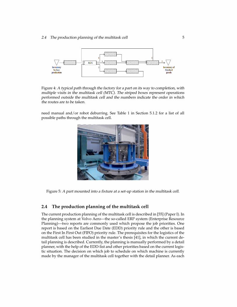
The parts that are ready to be processed in the multitask cell are those that arechecked-in at the input conveyor but not yet put into a fixture at a set-up station.After the check-in, the parts are transported by a stocker crane to special storagelocations inside the multitask cell. There are also storage areas inside the cell for partsthat are already mounted into fixtures. Each part to be processed in the multitaskcell follows a specific routing through the set of resources, which consists of three tofive so-called route operations, starting and ending by the mounting and removing offixtures at one of the three set-up stations; see Figure 5. The second route operationin this routing is always the processing in one of the multitask machines. Some parts
2.4 The production planning of the multitask cell 5
Figure 4: A typical path through the factory for a part on its way to completion, withmultiple visits in the multitask cell (MTC). The striped boxes represent operationsperformed outside the multitask cell and the numbers indicate the order in whichthe routes are to be taken.
need manual and/or robot deburring. See Table 1 in Section 5.1.2 for a list of allpossible paths through the multitask cell.
Figure 5: A part mounted into a fixture at a set-up station in the multitask cell.
2.4 The production planning of the multitask cell
The current production planning of the multitask cell is described in [55] (Paper I). Inthe planning system at Volvo Aero—the so-called ERP system (Enterprise ResourcePlanning)—two reports are commonly used which propose the job priorities. Onereport is based on the Earliest Due Date (EDD) priority rule and the other is basedon the First In First Out (FIFO) priority rule. The prerequisites for the logistics of themultitask cell has been studied in the master’s thesis [41], in which the current de-tail planning is described. Currently, the planning is manually performed by a detailplanner, with the help of the EDD-list and other priorities based on the current logis-tic situation. The decision on which job to schedule on which machine is currentlymade by the manager of the multitask cell together with the detail planner. As each

6 3 JOB SHOP SCHEDULING: A SUBJECT ORIENTATION
job is only allowed to be processed in a subset of the multitask machines, this is nota simple task: Even though the processing machines are of the same kind, they arenot identical, and some of the machines have been altered in order to be able to pro-cess some large parts. Also, some machines yield a result which are better repetitivefor certain jobs having requirements on extremely small tolerances on e.g. rotundityand thickness, due to flight safety issues. These are two of the reasons why somejobs can only be processed in some machines. Another reason is that some productsconsist of a different material than the rest, and the price paid by scrap dealers ismuch lower for mixed metal chips (the metal scrap from the turning process) thanfor sorted materials. This reason differs from the others, since it can be eliminatedby either scheduling a cleaning operation in a machine between any two operationscomprising parts of different materials, or selling the metal chips at the lower price.As a consequence of the low product volumes and the expensive machines, whichare difficult to move, most of the parts take different routes in the factory, such asthe one illustrated in Figure 4. Getting an overview of the planning situation withregard to incoming jobs is therefore difficult for a manual planner.
The problem described—to schedule the operations in the multitask cell—can beclassified as a flexible job shop problem in the operations research nomenclature. In thefollowing section, this problem is described in more general terms.
3 Job shop scheduling: A subject orientation
The job shop scheduling problem is one of three classic shop scheduling problems, theother two being the flow shop and the open shop scheduling problems; see [8]. The jobshop problem is defined as that to find the optimal sequences of a given set of jobson a given set of machines. Each job consists of a number of operations, which mustbe processed in a given order. The constraints indicating that one operation mustprecede another are called precedence constraints. Associated with each operation is ajob, a machine, and a processing time. The flexible job shop problem is an extensionof the job shop problem, in the sense that each operation may be scheduled in morethan oneof the machines; see [3].
3.1 The perspective of operations research
Operations research is an interdisciplinary science that focuses on the efficient useof technology in order to arrive at optimal, or near-optimal, solutions to complexdecision-making problems; see e.g. [50].
3.1.1 Mathematical optimization
The first integer programming formulations of job-shop problems were formulated inthe late 50’s by Manne ([33]), Wagner ([58]), and Bowman ([7]). These formulationsare all different, since they model the dimension of time in three different ways,which in turn reflect their respective definitions of the binary decision variables.
3.1 The perspective of operations research 7
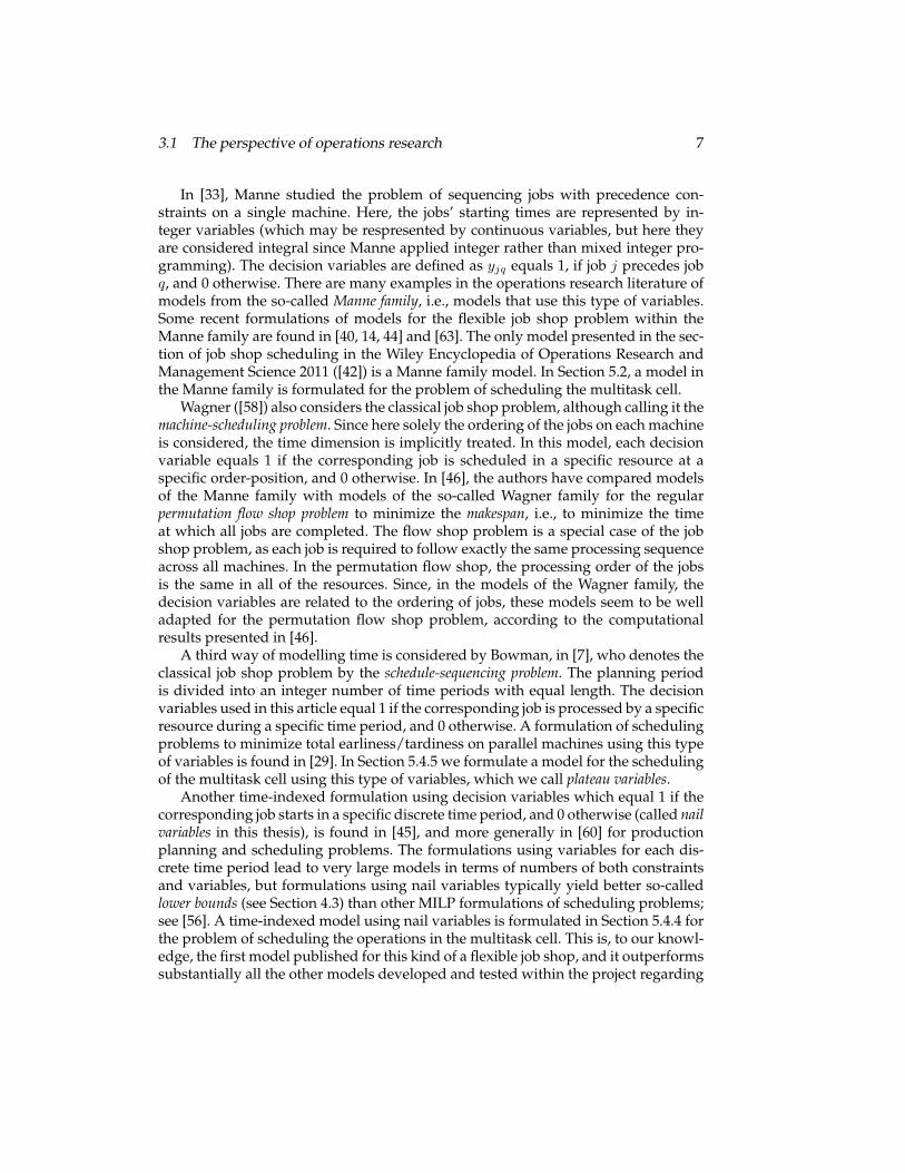
In [33], Manne studied the problem of sequencing jobs with precedence con-straints on a single machine. Here, the jobs’ starting times are represented by in-teger variables (which may be respresented by continuous variables, but here theyare considered integral since Manne applied integer rather than mixed integer pro-gramming). The decision variables are defined as yjq equals 1, if job j precedes jobq, and 0 otherwise. There are many examples in the operations research literature ofmodels from the so-called Manne family, i.e., models that use this type of variables.Some recent formulations of models for the flexible job shop problem within theManne family are found in [40, 14, 44] and [63]. The only model presented in the sec-tion of job shop scheduling in the Wiley Encyclopedia of Operations Research andManagement Science 2011 ([42]) is a Manne family model. In Section 5.2, a model inthe Manne family is formulated for the problem of scheduling the multitask cell.
Wagner ([58]) also considers the classical job shop problem, although calling it themachine-scheduling problem. Since here solely the ordering of the jobs on each machineis considered, the time dimension is implicitly treated. In this model, each decisionvariable equals 1 if the corresponding job is scheduled in a specific resource at aspecific order-position, and 0 otherwise. In [46], the authors have compared modelsof the Manne family with models of the so-called Wagner family for the regularpermutation flow shop problem to minimize the makespan, i.e., to minimize the timeat which all jobs are completed. The flow shop problem is a special case of the jobshop problem, as each job is required to follow exactly the same processing sequenceacross all machines. In the permutation flow shop, the processing order of the jobsis the same in all of the resources. Since, in the models of the Wagner family, thedecision variables are related to the ordering of jobs, these models seem to be welladapted for the permutation flow shop problem, according to the computationalresults presented in [46].
A third way of modelling time is considered by Bowman, in [7], who denotes theclassical job shop problem by the schedule-sequencing problem. The planning periodis divided into an integer number of time periods with equal length. The decisionvariables used in this article equal 1 if the corresponding job is processed by a specificresource during a specific time period, and 0 otherwise. A formulation of schedulingproblems to minimize total earliness/tardiness on parallel machines using this typeof variables is found in [29]. In Section 5.4.5 we formulate a model for the schedulingof the multitask cell using this type of variables, which we call plateau variables.
Another time-indexed formulation using decision variables which equal 1 if thecorresponding job starts in a specific discrete time period, and 0 otherwise (called nailvariables in this thesis), is found in [45], and more generally in [60] for productionplanning and scheduling problems. The formulations using variables for each dis-crete time period lead to very large models in terms of numbers of both constraintsand variables, but formulations using nail variables typically yield better so-calledlower bounds (see Section 4.3) than other MILP formulations of scheduling problems;see [56]. A time-indexed model using nail variables is formulated in Section 5.4.4 forthe problem of scheduling the operations in the multitask cell. This is, to our knowl-edge, the first model published for this kind of a flexible job shop, and it outperformssubstantially all the other models developed and tested within the project regarding
8 3 JOB SHOP SCHEDULING: A SUBJECT ORIENTATION
the computation time required to solve the problems and also regarding which sizesof instances they are able to solve within reasonable computation time.
The objective that is the most studied for scheduling problems is the minimiza-tion of makespan; see [27]. Other common objectives are related to the jobs’ earli-ness/tardiness and completion times, and/or inventory holding costs associatedwith the jobs. A model with a time-indexed formulation, in which the time-indexedvariables are integral and not binary, as in the time-indexed models mentioned above,is presented in [19]. The objective function in [19] is to minimize the costs associatedwith in-process inventory, earliness/tardiness and costs associated with orders notfully completed at the end of the scheduling horizon. See Section 5.1.5 for a discus-sion on different objective functions and their suitability for the planning of opera-tions in the multitask cell.
3.1.2 Metaheuristics
Integer linear programming models formulated for scheduling problems in the pe-riod of 1959–1990 are correct, but the computers were then able to solve only verysmall instances, and it was not possible to employ an exact mathematical optimiza-tion on instances of sizes relevant for real applications. Therefore, a lot of researchwas concentrated on obtaining an approximate solution of job shop problems by theapplication of heuristic methods; see [27] for an historical overview. According to[27], the development of so-called metaheuristics for job shop scheduling started withthe development of the so-called shifting bottleneck heuristic by Adams et al. in 1988([1]). Since then, many metaheuristics have been proposed for finding schedules forjob shops, among these are simulated annealing, tabu search, genetic algorithms, and antcolony optimization; see, e.g., [14, 62, 36] and [21] for some recently proposed hybridapproximation algorithms which are based on the metaheuristics mentioned above.A genetic algorithm for the job shop problem with the tardiness objective is foundin [35]. The shifting bottleneck heuristic is still popular; see [37] for a variant forthe flexible job shop, and [10] which combines the shifting bottleneck heuristic witha MILP model. Other recent work on the flexible job shop problem are [12, 59, 23]and [16], of which [59] also considers preventive maintenance activities.
The major disadvantage with metaheuristics is that there is often no other stop-ping criteria than a maximum allowed number of iterations, or limited computationtime. Hence, no quality measure of the solution is provided as for the case of ap-plying mathematical optimization. Therefore, the quality of the solutions obtainedbecome unknown. Another weakness of the approximation algorithms is that oftenthere are several parameters that have to be carefully selected in order for the algo-rithms to produce good solutions ([27]). Comparisons between different heuristicsoften become invalid since they are usually performed from an unbalanced perspec-tive: Typically, the approaches taken are presented with a very well calibrated setof parameter values, while other approaches included in the study for comparisons,are employed using a standard parameter setting. Hence, a fair comparison is oftennot achieved.
Arostegui et al. ([2]) have made an attempt to make a fair comparison between
3.2 The perspective of logistics 9
tabu search, simulated annealing, and genetic algorithms for three variants of thefacility location problem (FLP). FLP is a complex combinatorial optimization prob-lem, which is as hard to solve as the job shop problem, according to the authors. Inthis article, tabu search seems to be the best algorithm, with good performance forall three variants, while both simulated annealing and genetic algorithms sometimesget stuck in worse local minima, and hence perform badly for some variants.
Other approaches to find good solutions to the job shop problem is to combinesimulation models with meta-heuristics; see, e.g., [49], which is especially interest-ing since the case study in that article is the Volvo Aero multitask cell considered inthis thesis. A more general description of this method is found in [48]. Yet anotherapproach is the use of constraint programming; see, e.g., [6]. In [4], a hybrid algorithmwhich combines a tabu search algorithm with constraint programming is proposedfor the job shop problem and represents, according to the authors, the first occasionin which a constraint programming algorithm obtains a performance that is compet-itive with the best so-called local search algorithms (e.g., tabu search is a local searchalgorithm).
3.2 The perspective of logistics
According to ([11]) the discipline of logistics is the management of the flow of goodsand services between the point of origin and the point of consumption in order tomeet the requirements of customers. The term production logistics is used to describelogistic processes in-house a factory [57]. The purpose of production logistics is toensure that each machine and workstation is being fed with the right product of thecorrect quantity and quality at the right time. This corresponds approximately to thegoal of the job shop problem, and although quality is seldom explicitly dealt withinthe scheduling community of operations research, the two disciplines have a lot incommon.
Scientific articles related to production planning written in the view of produc-tion logistics typically do not have an as quantitative perspective as those written inthe view of operations research. For example, Stoop and Wiers ([47]) list a number ofcauses for automated scheduling techniques not functioning in practice. Such causescan be disturbances, machine breakdowns, rush orders, or the unavailability of rawmaterials. Another cause can be personnel overruling the scheduling tools, believingthat they can outperform the technique. It is hard to prove to personnel responsiblefor operations planning the advantages of an automated scheduling technique, sincethe quality of a schedule is usually very hard to assess.
In [22], Herrmann describes production scheduling from a logistics point of view,and with a hierarchical view of the organizational, decision-making, and problem-solving perspectives of production scheduling. In this view, the problem of findingoptimal schedules equals production scheduling from the problem-solving perspec-tive. In the decision-making perspective, the schedulers also perform tasks such ascrisis identification, and make decisions in order to avoid possible future trouble.The broadest perspective is the organizational perspective, which takes the wholeorganization around the production into account. The author points out that pro-
10 4 ON THE COMPLEXITY OF SCHEDULING PROBLEMS
duction scheduling is not just an optimization problem, but a complex system ofinformation flow, decision-making, and problem-solving.
Although job shop scheduling is complex, feasible schedules are found every dayall around the world for all the various real applications that need to be scheduled.The most common means for constructing a schedule is to make use of one of manydispatching rules, proposed by, e.g. [5] and [24]. A dispatching rule (also called priorityrule) is classified as a static rule if the priority value once calculated remains the samethroughout the planning horizon; it is called a dynamic rule if the priority value cal-culated at a certain point in time differs from that calculated at a later time. The mostcommon static rules are the so-called shortest–processing–time (SPT), earliest–due–date(EDD) and first–in–first–out (FIFO); a description of these and other dispatching rulescan be found in e.g. [25].
In this work, the schedules generated by static dispatching rules applied to datafrom real instances from the multitask cell have been compared with the resultingschedules emanating from the mathematical optimization models presented in Sec-tions 5.3 and 5.4.4, for the same set of instances. The results from these comparisonsare reported in Section 6, in [55] (Paper I in this thesis), and in [52].
The priority lists resulting from the use of dispatching rules can be generated bycommercial planning softwares, henceforth called ERP (Enterprise Resource Plan-ning) systems. Other commercial planning softwares include the more sofisticatedAPS (Advanced Planning and Scheduling) systems, which are often integrated withthe ERP systems; see e.g. [25, pp. 147–149]. APS systems are, however, usually de-signed to cover all the different classes of scheduling problems—e.g. job shop, flowshop, open shop, assembly line, and continuous flow (e.g. process industry) schedul-ing problems—and, therefore, they typically offer only a small number of genericscheduling algorithms. The disadvantage of the commercial planning softwares isthat a built-in generic scheduling algorithm probably most often results in worseschedules than does a tailored scheduling algorithm for a certain problem class, suchas, e.g., flexible job shop ([31]).
4 On the complexity of scheduling problems
Scheduling problems such as flow shop, job shop, and open shop problems havebeen known to be NP-complete since the mid seventies ([18]). An NP-complete orNP-hard problem is such that no algorithm exists that in polynomial time is ableto solve all possible instances of the problem ([17]). Hence, the solution time risksto increase exponentially with the number of jobs. The difference between the no-tions NP-hard and NP-complete is that NP-hard problems are at least as hard as NP-complete problems; see [17, p. 109]. In [18], the flow shop problem with the objectiveof minimizing makespan was proven to be NP-complete for instances with three ormore machines. It was also shown that the flow shop problem with the objective ofminimizing the mean flow time, i.e., the sum of the jobs’ completion times, and thejob shop problem with the makespan criterion, are NP-complete for instances withtwo or more machines.
4.1 On the complexity of flow shop problems with deteriorating jobs 11
4.1 On the complexity of flow shop problems with deterioratingjobs
In [53] (Paper II in this thesis), we present a proof of NP-hardness for flow shopproblems for which the processing time of each job is equal to a deterioration ratetimes the job’s starting time. It is a note on an article written by Mosheiov in 2002([38]), in which the proof regarding the complexity of a flow shop problem withdeteriorating jobs is incorrect. We provide a correct proof of the statement that thisproblem is NP-hard for instances with three or more machines, when the objectiveis to minimize the makespan.
During the work with this note, it came to our notice that a correct proof, foran even stronger result, was published already in 1996 in a Russian journal; seeKononov [30]. This proof, originally given in Russian, is summarized in [53] (Pa-per II). However, we noted, while tracing the citation history of the two proofsby Mosheiov and Kononov, respectively, that the incorrect proof by Mosheiov wasby far the one most often cited. Hence, we considered a correction of the proof byMosheiov being necessary and quite timely.
4.2 On the complexity of flexible job shop problems
We consider here a subproblem of the flexible job shop problem studied in this the-sis, namely scheduling only the five processing machines in the multitask cell. Wefurther assume that all parts to be scheduled are available from the start, i.e., all re-lease dates are set to zero for all jobs, and that there are no precedence constraintsbetween the jobs. Moreover, we consider the objective of minimizing the weightedsum of completion times.
Using the α|β|γ-notation introduced in [20], this problem can then be describedas F MPM5|stages = 1|
∑wiCi. The first field, α, specifies the machine environment,
where F, J, and O denote flow shop, job shop and open shop, respectively. Thesenotations can be combined with, e.g. P and MPM, which denote identical parallellmachines, and multi-purpose machines, respectively, and a number k, representingthe number of machines. The subproblem considered above has only one stage, thatis, each job consists of one operation. Therefore, the first element of α can be set toany of F, J, and O. We have chosen α = ”F MPM5” for convenience.
The β-field is used to describe the job characteristics. There can be at most sixelements in this field, for example prec, ri, or di for precedence constraints, releasedates and due dates, respectively, to name a few elements relevant to the problemsstudied in this thesis. In the subproblem considered here, these job characteristicsare not relevant due to the assumptions made above. We therefore set β equal tostages= 1.
The last field in this notation is the γ-field which is used to describe the opti-mality criterion. The most common objective functions are the minimization of themakespan (γ = Cmax), total completion times (γ =
∑Ci) and weighted completion
times (γ =∑wiCi). Note that the indices on the
∑-symbol are skipped in this nota-
tion. Other notations of interest are Ei and Ti which denote earliness and tardiness,
12 4 ON THE COMPLEXITY OF SCHEDULING PROBLEMS
respectively. For further explanation of the α|β|γ-notation; see e.g. [8].The considered subproblem (F MPM5|stages = 1|
∑wiCi) of the flexible job shop
problem is a generalization of the problem P5||∑wiCi, i.e., the problem of schedul-
ing five parallell machines with the weighted completion times criterion; see [9].Since the problem Pk||
∑wiCi has been shown to be NP-hard for k ≥ 2 ([17]), it
follows that the subproblem considered (F MPM5|stages = 1|∑wiCi) is NP-hard
(k = 5). Since this subproblem is a special case of the problem studied in this thesis,we can conclude that the problem of scheduling the multitask cell is NP-hard.
4.3 Weak and strong formulations
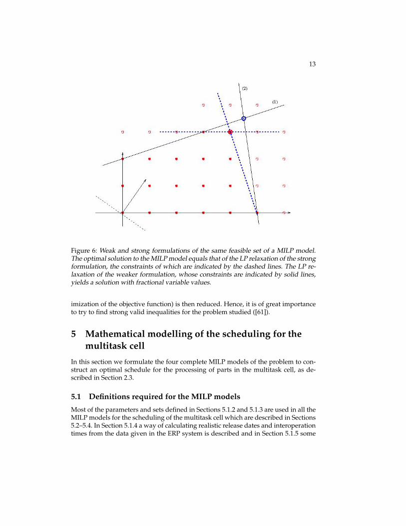
Since we are dealing with NP-hard problems the computation times may becomevery long, as mentioned in the beginning of this section, and hence the choices ofboth the solution algorithm and the problem formulation are of great importance.In this thesis we have chosen to use a state-of-the-art optimization software, and letthis software make the choice of solution algorithm. Instead, we made an effort todevelop good mixed integer linear programming (MILP) models for the problem ofscheduling the multitask cell. The MILP models are formulated with both integer (orbinary) and continuous variables, and with all the relations between the variables inthe objective and constraints being linear ([39]). For linear programs (LP), in whichall variables are continuous, an optimal solution, if it exists, is found at an extremepoint of the feasible region (the polyhedron defined by the linear relations betweenthe continuous variables). This is, however, not the case for MILP models, since theextreme points may contain fractional variable values. A lower bound on the valueof the optimal MILP solution is found when solving the so-called LP relaxation of theproblem, i.e. when relaxing all integer and/or binary constraints on the variables.The constraints formulated to describe the feasible region of a MILP model are calledstrong, if the objective value of the corresponding LP relaxation is close to that ofthe optimal solution; it is called weak, if the constraints in the LP relaxation yield asolution whose objective value is far from that of the corresponding optimal solution.An example is given in 2D in Figure 6.
In the example in Figure 6, the feasible set of the MILP model is illustrated bysmall filled circles. Both variables are subject to non-negativity constraints, and thereare two sets of the remaining constraints corresponding to a weak and a strong for-mulation, respectively, of the MILP model. The constraints in the weak formulationare illustrated with solid lines, and those in the strong formulation by dashed lines.The constraint marked with (1) in the figure is valid for both formulations. The arrowindicates the direction of decreasing objective function values. The optimal solutionof the MILP model equals that of the LP relaxation of the strong formulation, i.e.,the intersection of the two dashed lines. The LP relaxation of the weak formulationyields an optimal solution with fractional variable values, i.e., the intersection of thelines marked (1) and (2) in Figure 6.
With the help of so-called strong valid inequalities, it is possible to cut off frac-tional solutions from the feasible region. The gap between the optimal value andthe optimal value of the corresponding continuous relaxation (considering the min-
13
Figure 6: Weak and strong formulations of the same feasible set of a MILP model.The optimal solution to the MILP model equals that of the LP relaxation of the strongformulation, the constraints of which are indicated by the dashed lines. The LP re-laxation of the weaker formulation, whose constraints are indicated by solid lines,yields a solution with fractional variable values.
imization of the objective function) is then reduced. Hence, it is of great importanceto try to find strong valid inequalities for the problem studied ([61]).
5 Mathematical modelling of the scheduling for themultitask cell
In this section we formulate the four complete MILP models of the problem to con-struct an optimal schedule for the processing of parts in the multitask cell, as de-scribed in Section 2.3.
5.1 Definitions required for the MILP models
Most of the parameters and sets defined in Sections 5.1.2 and 5.1.3 are used in all theMILP models for the scheduling of the multitask cell which are described in Sections5.2–5.4. In Section 5.1.4 a way of calculating realistic release dates and interoperationtimes from the data given in the ERP system is described and in Section 5.1.5 some
14 5 MATHEMATICAL MODELLING
different objective functions are discussed.
5.1.1 Assumptions made for the mathematical formulations
All the processing tools for the multitask cell are assumed to be available and trans-ported to the appropriate resource on time for each route operation. The numberof available fixtures is not a limiting factor at present in the multitask cell and it istherefore assumed to be unlimited. For some of the operations, namely, mountinginto fixtures, manual deburring, and removing parts from the fixtures, personnel arerequired during the entire operation, while most of the processing operations re-quire manual work only during a fraction of the operation processing time. Thereare also other tasks regarding, for example, the machining tools, that the personnelare expected to perform simultaneously with their work with the route operationsin the multitask cell. As mentioned in Section 1.3, the availability of personnel forthe manual work of the cell is here considered to be sufficient, but in practice thiswill not always be the case, especially not if the work load of the cell is considerablyincreased in comparison with the current situation; therefore, we plan to includemanpower planning in the future research. The availability of storage before and be-tween the resources is assumed to be unlimited. The assumptions made above are,however, not always true; how they best can be included in the mathematical modelsis an area for future studies.
5.1.2 Indices and definitions of sets
In order to acquire the appropriate parameter data for the MILP models, the jobsthat are to be processed in the multitask cell must be studied and categorized. Theycan be divided into three categories, since each order (part) passes through threedifferent phases before its processing in the multitask cell. These are
1. planned orders not yet released, i.e. orders that exist in the planning systemonly;
2. released orders, or so-called production orders, i.e. physical parts being pro-cessed outside the cell on their way to the multitask cell; and
3. jobs checked-in into the multitask cell, i.e. parts inside the multitask cell wait-ing to be processed.
The whole set of jobs to be processed during the planning period considered,i.e. the queue of jobs, is denoted by J . Some of these jobs are to be processed on thesame physical part; hence, there are two categories of jobs in phases 2 and 3. The firstcategory is characterized by the part being inside or on its way to the multitask cellfor the processing of the corresponding job. The second category is characterizedby the part being inside or on its way to the multitask cell for the processing of apreceding job in the routing, before making another round through the factory and,finally, reaching the multitask cell for the processing of the job in question.

5.1 Definitions required for the MILP models 15
As an example of the second category, consider a job q ∈ J being the job to beprocessed at a part’s third visit to the multitask cell, as illustrated in Figure 4, whilethe physical part, on which job q is going to be performed, is on its way to visit themultitask cell for the second time, for processing of job j ∈ J . Another example, asfor the jobs q and l illustrated in Figure 7, occurs when no operations are requiredoutside the multitask cell before the processing of the next job. The pairs of all jobsadjacent in the routing form the product setQ ⊂ J ×J . For the part, whose routingis illustrated in Figure 7, the pairs (j, q) and (q, l) belongs to the set Q.
Figure 7: Routing of a part in the factory with jobs j, q, and l to be processed in themultitask cell. The set of pairs {(j, q), (q, l)} ⊆ Q.
Each job j consists of nj operations i, i.e., i ∈ Nj = {1, . . . , nj}, to be processedinside the multitask cell. The route operations that can be performed inside the cellare listed in Table 1, together with the four possible variants of the ordering of theroute operations belonging to the set Nj for a job j. Note that the route operationsi = 1, 2 are of the same kind for all the jobs.
Description of operation Job type(i) (ii) (iii) (iv)
mounting into fixture 1 1 1 1turning/milling/drilling 2 2 2 2manual deburring 3 3automatic deburring 4 3removing from fixture 5 4 4 3
Table 1: Each job, j, consists of an ordered set of route operations that are performedinside the multitask cell. There are four variants, here denoted (i),. . . ,(iv), of thesesets, which are mathematically denoted by Nj , j ∈ J .
The route operations are performed in the ten processing resources in the multi-task cell. The first (i = 1) and the last (i = nj) route operations are always performedin one of the three set-up/tear-down stations. The set of k resources is denoted byK,and the set of multitask machines is denoted by K ⊂ K. All the resources consideredfor scheduling in the thesis are listed in Table 2.
5.1.3 Definition of parameters and time variables
Linked with each route operation i of job j, henceforth denoted operation (i, j), andeach resource k, is a parameter λijk, which equals 1 if operation (i, j) is allowed to
16 5 MATHEMATICAL MODELLING
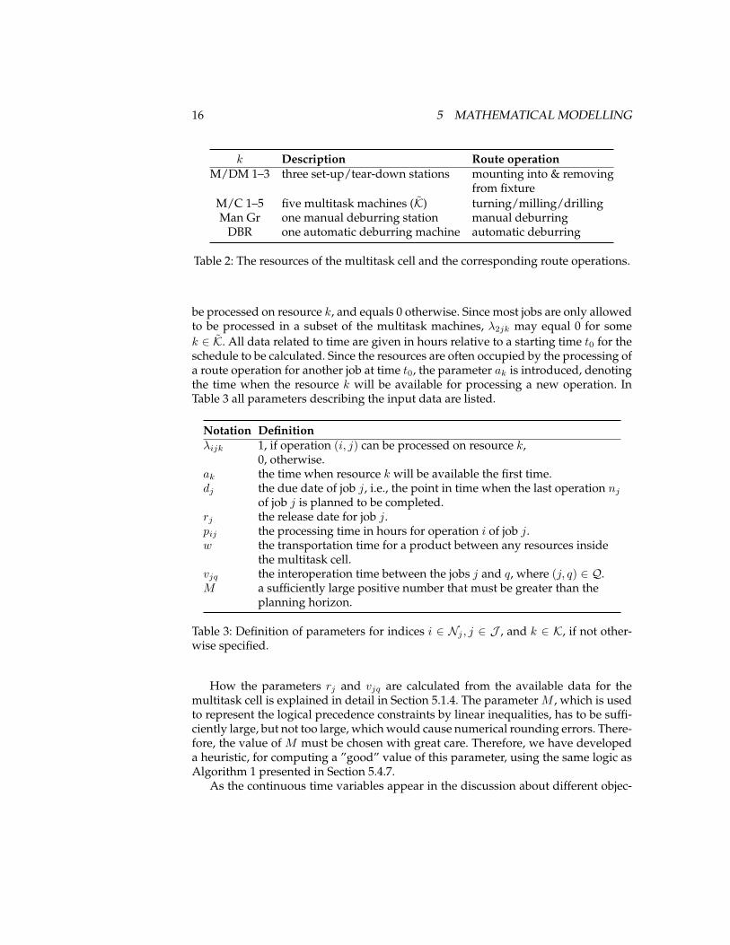
k Description Route operationM/DM 1–3 three set-up/tear-down stations mounting into & removing
from fixtureM/C 1–5 five multitask machines (K) turning/milling/drillingMan Gr one manual deburring station manual deburring
DBR one automatic deburring machine automatic deburring
Table 2: The resources of the multitask cell and the corresponding route operations.
be processed on resource k, and equals 0 otherwise. Since most jobs are only allowedto be processed in a subset of the multitask machines, λ2jk may equal 0 for somek ∈ K. All data related to time are given in hours relative to a starting time t0 for theschedule to be calculated. Since the resources are often occupied by the processing ofa route operation for another job at time t0, the parameter ak is introduced, denotingthe time when the resource k will be available for processing a new operation. InTable 3 all parameters describing the input data are listed.
Notation Definitionλijk 1, if operation (i, j) can be processed on resource k,
0, otherwise.ak the time when resource k will be available the first time.dj the due date of job j, i.e., the point in time when the last operation nj
of job j is planned to be completed.rj the release date for job j.pij the processing time in hours for operation i of job j.w the transportation time for a product between any resources inside
the multitask cell.vjq the interoperation time between the jobs j and q, where (j, q) ∈ Q.M a sufficiently large positive number that must be greater than the
planning horizon.
Table 3: Definition of parameters for indices i ∈ Nj , j ∈ J , and k ∈ K, if not other-wise specified.
How the parameters rj and vjq are calculated from the available data for themultitask cell is explained in detail in Section 5.1.4. The parameter M , which is usedto represent the logical precedence constraints by linear inequalities, has to be suffi-ciently large, but not too large, which would cause numerical rounding errors. There-fore, the value of M must be chosen with great care. Therefore, we have developeda heuristic, for computing a ”good” value of this parameter, using the same logic asAlgorithm 1 presented in Section 5.4.7.
As the continuous time variables appear in the discussion about different objec-
5.1 Definitions required for the MILP models 17
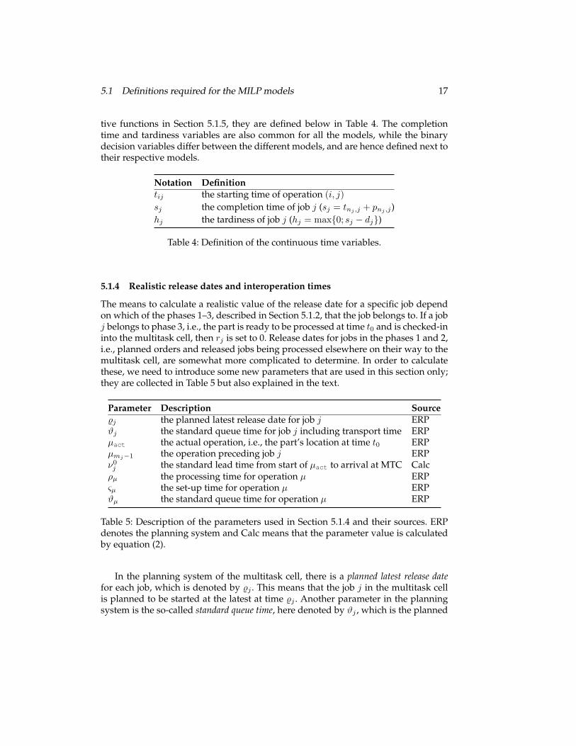
tive functions in Section 5.1.5, they are defined below in Table 4. The completiontime and tardiness variables are also common for all the models, while the binarydecision variables differ between the different models, and are hence defined next totheir respective models.
Notation Definitiontij the starting time of operation (i, j)
sj the completion time of job j (sj = tnj ,j + pnj ,j)hj the tardiness of job j (hj = max{0; sj − dj})
Table 4: Definition of the continuous time variables.
5.1.4 Realistic release dates and interoperation times
The means to calculate a realistic value of the release date for a specific job dependon which of the phases 1–3, described in Section 5.1.2, that the job belongs to. If a jobj belongs to phase 3, i.e., the part is ready to be processed at time t0 and is checked-ininto the multitask cell, then rj is set to 0. Release dates for jobs in the phases 1 and 2,i.e., planned orders and released jobs being processed elsewhere on their way to themultitask cell, are somewhat more complicated to determine. In order to calculatethese, we need to introduce some new parameters that are used in this section only;they are collected in Table 5 but also explained in the text.
Parameter Description Source%j the planned latest release date for job j ERPϑj the standard queue time for job j including transport time ERPµact the actual operation, i.e., the part’s location at time t0 ERPµmj−1 the operation preceding job j ERPν0j the standard lead time from start of µact to arrival at MTC Calcρµ the processing time for operation µ ERPςµ the set-up time for operation µ ERPϑµ the standard queue time for operation µ ERP
Table 5: Description of the parameters used in Section 5.1.4 and their sources. ERPdenotes the planning system and Calc means that the parameter value is calculatedby equation (2).
In the planning system of the multitask cell, there is a planned latest release datefor each job, which is denoted by %j . This means that the job j in the multitask cellis planned to be started at the latest at time %j . Another parameter in the planningsystem is the so-called standard queue time, here denoted by ϑj , which is the planned
18 5 MATHEMATICAL MODELLING
time between the completion of the preceding operation performed outside the mul-titask cell and the latest release date %j , including the time for the transport to themultitask cell. The desired release date, rj , that should be included in the optimizationmodel, should, however, be a realistic estimation of the point in time when the partarrives to the multitask cell. Therefore, a fraction of the standard queue time must besubtracted from %j . A measure that is often used at Volvo Aero is the transport timeconstituting about 20% of the standard queue time; hence we choose to compute rjas
rj = max{%j − 0.8ϑj − t0; ν0j }, (1)
where ν0j is the standard lead time from the preceding operation on the part to be
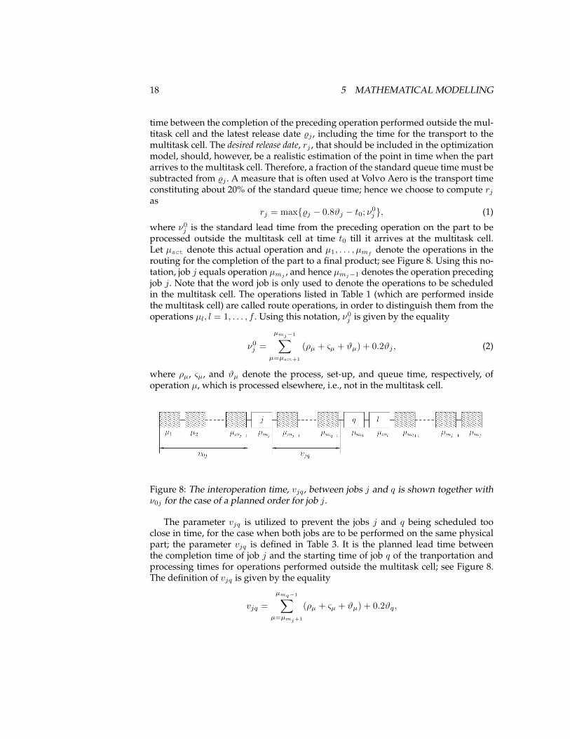
processed outside the multitask cell at time t0 till it arrives at the multitask cell.Let µact denote this actual operation and µ1, . . . , µmf
denote the operations in therouting for the completion of the part to a final product; see Figure 8. Using this no-tation, job j equals operation µmj
, and hence µmj−1 denotes the operation precedingjob j. Note that the word job is only used to denote the operations to be scheduledin the multitask cell. The operations listed in Table 1 (which are performed insidethe multitask cell) are called route operations, in order to distinguish them from theoperations µl, l = 1, . . . , f . Using this notation, ν0
j is given by the equality
ν0j =
µmj−1∑µ=µact+1
(ρµ + ςµ + ϑµ) + 0.2ϑj , (2)
where ρµ, ςµ, and ϑµ denote the process, set-up, and queue time, respectively, ofoperation µ, which is processed elsewhere, i.e., not in the multitask cell.
Figure 8: The interoperation time, vjq , between jobs j and q is shown together withν0j for the case of a planned order for job j.
The parameter vjq is utilized to prevent the jobs j and q being scheduled tooclose in time, for the case when both jobs are to be performed on the same physicalpart; the parameter vjq is defined in Table 3. It is the planned lead time betweenthe completion time of job j and the starting time of job q of the tranportation andprocessing times for operations performed outside the multitask cell; see Figure 8.The definition of vjq is given by the equality
vjq =
µmq−1∑µ=µmj+1
(ρµ + ςµ + ϑµ) + 0.2ϑq,
5.1 Definitions required for the MILP models 19
where ρµ, ςµ, and ϑµ denote respectively the process, set-up and queue times of op-eration µ, which is processed elsewhere (cf. (2)). As mentioned before, 0.2ϑq is theestimated transport time to the multitask cell from the operation preceding job q forthis physical part.
5.1.5 Objectives for the scheduling of the multitask cell
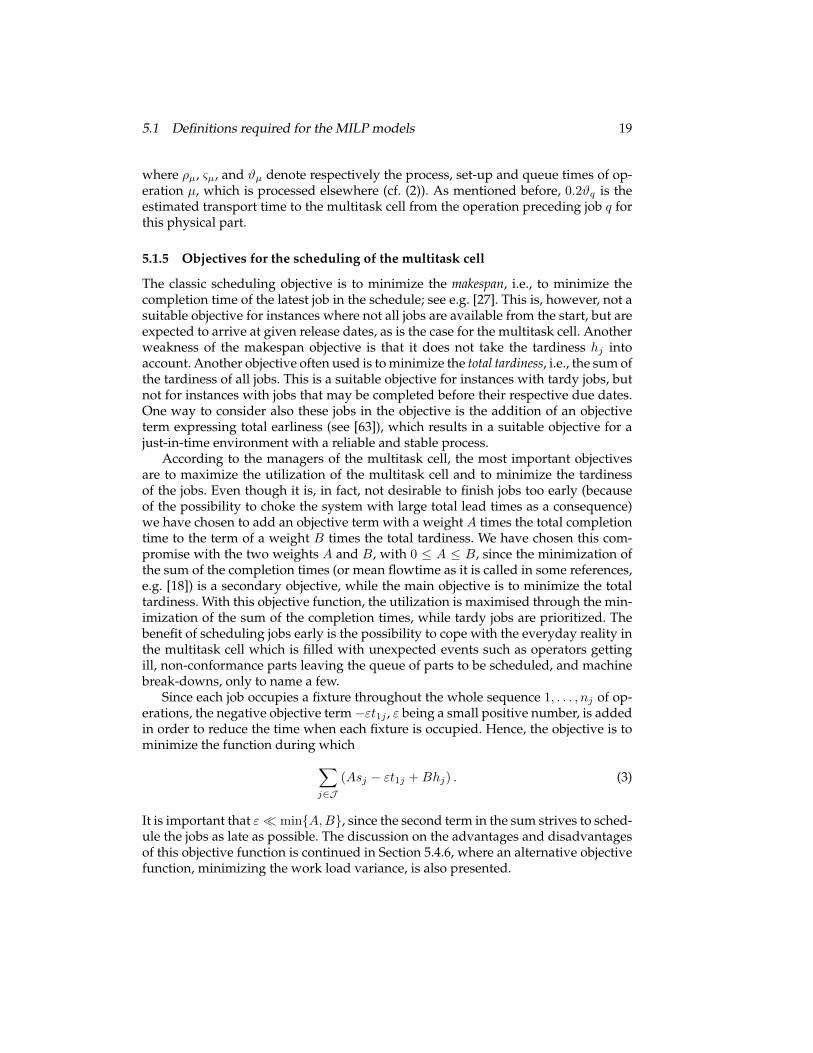
The classic scheduling objective is to minimize the makespan, i.e., to minimize thecompletion time of the latest job in the schedule; see e.g. [27]. This is, however, not asuitable objective for instances where not all jobs are available from the start, but areexpected to arrive at given release dates, as is the case for the multitask cell. Anotherweakness of the makespan objective is that it does not take the tardiness hj intoaccount. Another objective often used is to minimize the total tardiness, i.e., the sum ofthe tardiness of all jobs. This is a suitable objective for instances with tardy jobs, butnot for instances with jobs that may be completed before their respective due dates.One way to consider also these jobs in the objective is the addition of an objectiveterm expressing total earliness (see [63]), which results in a suitable objective for ajust-in-time environment with a reliable and stable process.
According to the managers of the multitask cell, the most important objectivesare to maximize the utilization of the multitask cell and to minimize the tardinessof the jobs. Even though it is, in fact, not desirable to finish jobs too early (becauseof the possibility to choke the system with large total lead times as a consequence)we have chosen to add an objective term with a weight A times the total completiontime to the term of a weight B times the total tardiness. We have chosen this com-promise with the two weights A and B, with 0 ≤ A ≤ B, since the minimization ofthe sum of the completion times (or mean flowtime as it is called in some references,e.g. [18]) is a secondary objective, while the main objective is to minimize the totaltardiness. With this objective function, the utilization is maximised through the min-imization of the sum of the completion times, while tardy jobs are prioritized. Thebenefit of scheduling jobs early is the possibility to cope with the everyday reality inthe multitask cell which is filled with unexpected events such as operators gettingill, non-conformance parts leaving the queue of parts to be scheduled, and machinebreak-downs, only to name a few.
Since each job occupies a fixture throughout the whole sequence 1, . . . , nj of op-erations, the negative objective term−εt1j , ε being a small positive number, is addedin order to reduce the time when each fixture is occupied. Hence, the objective is tominimize the function during which∑
j∈J(Asj − εt1j +Bhj) . (3)
It is important that ε� min{A,B}, since the second term in the sum strives to sched-ule the jobs as late as possible. The discussion on the advantages and disadvantagesof this objective function is continued in Section 5.4.6, where an alternative objectivefunction, minimizing the work load variance, is also presented.
20 5 MATHEMATICAL MODELLING
5.2 The full engineer’s model
In this section we present a mixed integer optimization model for the full problem,i.e., for the whole multitask cell including all ten resources. This model belongs tothe Manne family (see Section 3.1.1), and is called the full engineer’s model, since it isa quite intuitive model for the whole multitask cell.
5.2.1 Definition of variables
The time variables used in this model are the continuous variables defined in Sec-tion 5.1.3 for starting, completion, and tardiness of a job. There are two sets of binarydecision variables in this model, namely zijk, which determines to which resource acertain operation is allocated, and yijpqk, denoting the precedence relations betweenthe operations. They are defined as
zijk =
{1, if operation (i, j) is allocated to resource k,0, otherwise,
yijpqk =
{1, if op (i, j) is processed before op (p, q) on resource k,0, otherwise,
for i, p ∈ Nj , j, q ∈ J , such that (i, j) 6= (p, q), and k ∈ K, and where ”op (i, j)”denotes route operation i of job j.
5.2.2 The engineer’s mathematical optimization model
Given the parameters and sets defined in Section 5.1.2 and the objective function (3)given in Section 5.1.5, the problem to schedule the multitask cell is formulated asthat to
minimize∑j∈J
(Asj − εt1j +Bhj) (4a)
subject to∑k∈K
zijk = 1, i ∈ Nj , j ∈ J , (4b)
zijk ≤ λijk, i ∈ Nj , j ∈ J , k ∈ K, (4c)yijpqk + ypqijk ≤ zijk, i ∈ Nj , p ∈ Nq, j, q ∈ J , (4d)
(i, j) 6= (p, q), k ∈ K,yijpqk + ypqijk + 1 ≥ zijk + zpqk, i ∈ Nj , p ∈ Nq, j, q ∈ J , (4e)
(i, j) 6= (p, q), k ∈ K,tij + pij −M(1− yijpqk) ≤ tpq, i ∈ Nj , p ∈ Nq, j, q ∈ J , (4f)
(i, j) 6= (p, q), k ∈ K,tij + pij + w ≤ ti+1,j , i ∈ Nj \ {nj}, j ∈ J , (4g)
t1j ≥ rj , j ∈ J , (4h)tij ≥ akzijk, j ∈ J , k ∈ K, (4i)t1q ≥ sj + vjq, (j, q) ∈ Q, (4j)
sj − tnjj = pnjj , j ∈ J , (4k)
5.2 The full engineer’s model 21
hj ≥ sj − dj , j ∈ J , (4l)hj ≥ 0, j ∈ J , (4m)tij ≥ 0, i ∈ Nj , j ∈ J , (4n)zijk ∈ {0, 1}, i ∈ Nj , j ∈ J , k ∈ K, (4o)
yijpqk ∈ {0, 1}, i ∈ Nj , p ∈ Nq, j, q ∈ J , (4p)(i, j) 6= (p, q), k ∈ K.
The constraints (4b) ensure that every operation is processed exactly once, and theconstraints (4c) make sure that each operation is scheduled on a resource allowed forthis specific operation. The constraints (4d) and (4e) induce an unambiguous order-ing of the operations that are to be processed in the same resource. The constraints(4d) make sure that yijpqk and ypqijk do not both equal 1; i.e., if operation (i, j) pre-cedes operation (p, q), operation (p, q) cannot precede operation (i, j). If operations(i, j) and (p, q) are to be performed on the same machine, then the constraints (4e)regulate that one of yijpqk and ypqijk must possess the value 1.
Furthermore, the constraints (4f) make sure that the starting time of operation(p, q) is scheduled after the completion of the previous operation in the same re-source. The parameter M is a big number, whose purpose is to relax the constraintswhenever yijpqk is valued zero, i.e., when the operations are not scheduled for pro-cessing in the same resource. See Section 6.2.4 for an analysis on the impact of dif-ferent values of M on the computation time. Generally, in scheduling problems theconstraints tpq + ppq −Myijpqk ≤ tij , being symmetric to the constraints (4f), arerequired, as e.g., in [40], but these become redundant here since yijpqk and ypqijk areregulated by the inequalities (4d) and (4e). The effect of an alternative formulationof these constraints for the engineer’s model for the five multitask machines is dis-cussed in Section 5.3.1.
The constraints (4g) ensure that the operations within the same job j are sched-uled in the correct order and that each operation is not scheduled until the previousoperation has been completed and the corresponding part transported to the currentresource in the set Nj . The constraints (4h) regulate the starting time of the first op-eration of every job, so that no job is scheduled prior to its release date. Moreover,the constraints (4i) make sure that no operation is scheduled in any resource beforethe resource is available for the first time. Any pair of two jobs, (j, q), say, belongingto the set Qmust be separated at least by the planned interoperation time vjq ; this isindicated by the constraints (4j). The completion time and the tardiness of each job jare defined by the constraints (4k)–(4m). Note that the nonnegativity constraints (4n)for the starting times are redundant due to equations (4g)–(4i) whenever the releasedate rj is nonnegative.
5.2.3 Preliminary computations using the full engineer’s model
Tests performed on real data instances with this model on a 4 Gb quad-core IntelXeon 3.2 GHz system using AMPL-CPLEX12 [15, 26] as optimization software, wereable to solve very small instances with 10 jobs to optimality within 3 minutes, but forinstances of 15 jobs, the computation times were as high as three months; see [52].
22 5 MATHEMATICAL MODELLING
5.3 The machining/feasibility problem decomposition
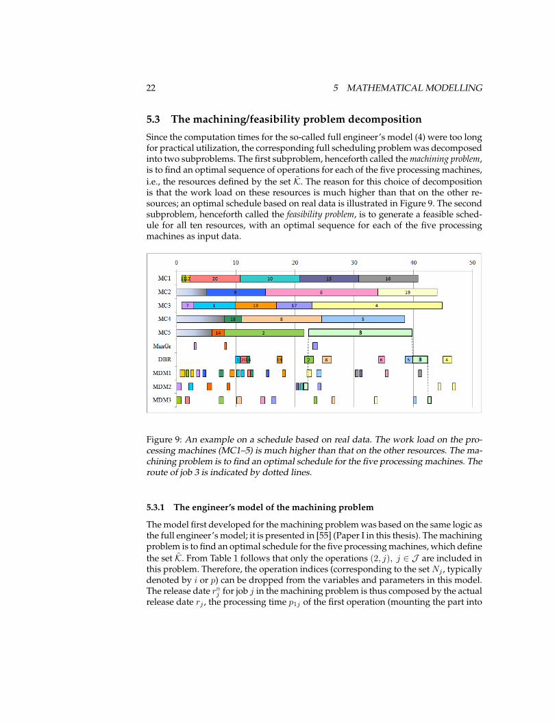
Since the computation times for the so-called full engineer’s model (4) were too longfor practical utilization, the corresponding full scheduling problem was decomposedinto two subproblems. The first subproblem, henceforth called the machining problem,is to find an optimal sequence of operations for each of the five processing machines,i.e., the resources defined by the set K. The reason for this choice of decompositionis that the work load on these resources is much higher than that on the other re-sources; an optimal schedule based on real data is illustrated in Figure 9. The secondsubproblem, henceforth called the feasibility problem, is to generate a feasible sched-ule for all ten resources, with an optimal sequence for each of the five processingmachines as input data.
Figure 9: An example on a schedule based on real data. The work load on the pro-cessing machines (MC1–5) is much higher than that on the other resources. The ma-chining problem is to find an optimal schedule for the five processing machines. Theroute of job 3 is indicated by dotted lines.
5.3.1 The engineer’s model of the machining problem
The model first developed for the machining problem was based on the same logic asthe full engineer’s model; it is presented in [55] (Paper I in this thesis). The machiningproblem is to find an optimal schedule for the five processing machines, which definethe set K. From Table 1 follows that only the operations (2, j), j ∈ J are included inthis problem. Therefore, the operation indices (corresponding to the set Nj , typicallydenoted by i or p) can be dropped from the variables and parameters in this model.The release date rmj for job j in the machining problem is thus composed by the actualrelease date rj , the processing time p1j of the first operation (mounting the part into

5.3 The machining/feasibility problem decomposition 23
a fixture), and the internal transportation time w, i.e.,
rmj = rj + p1j + w, j ∈ J . (5)
Accordingly, the resulting completion times are adjusted by the time required for theprocessing of the post-machining operations and the corresponding internal trans-ports as
ppmj =
nj∑i=3
(pij + w), j ∈ J ,
so that it reflects the completion of the whole job, including all the operations in-cluded. The parameters ak, dj , and M are unchanged and are thus as defined inTable 3, and the remaining parameters are redefined according to
λjk := λ2jk, j ∈ J , k ∈ K, (6a)pj := p2j , j ∈ J , (6b)vmjq := vjq + p1q + w, (j, q) ∈ Q. (6c)
The variables of the engineer’s model are also redefined so that they represent thesecond operation of the jobs, except for the completion time sj and the tardiness hjof job j, which are kept related to the end of the last operation of the job. Hence, thevariables are defined as
zjk =
{1, if op (2, j) is allocated to resource k,0, otherwise,
j ∈ J , k ∈ K,
yjqk =
{1, if op (2, j) is processed before op (2, q) on resource k,0, otherwise,
j, q ∈ J , k ∈ K,
tj = the starting time of op (2, j), j ∈ J ,sj = tj + p2j + ppmj , i.e., the completion time of job j, j ∈ J ,hj = max{0; sj − dj}, i.e., the tardiness of job j, j ∈ J ,
where op (2, j) denotes the machining operation of job j. Since the machining prob-lem deals with scheduling only the second operation, the second term in the ob-jective function (3) are not applicable here. The engineer’s model of the machiningproblem is thus to
minimize∑j∈J
(Asj +Bhj), (7a)
subject to∑k∈K
zjk = 1, j ∈ J , (7b)
zjk ≤ λjk, j ∈ J , k ∈ K, (7c)
yjqk + yqjk ≤ zjk, j, q ∈ J , j 6= q, k ∈ K, (7d)
yjqk + yqjk + 1 ≥ zjk + zqk, j, q ∈ J , j 6= q, k ∈ K, (7e)
24 5 MATHEMATICAL MODELLING
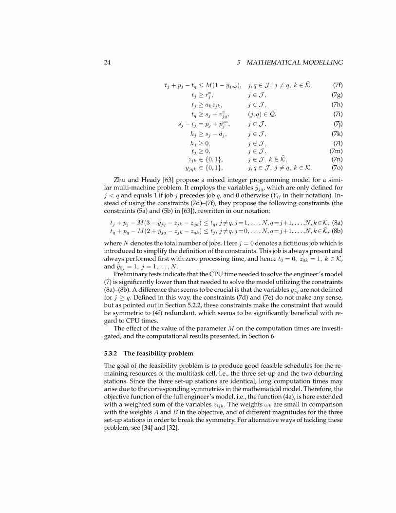
tj + pj − tq ≤M(1− yjqk), j, q ∈ J , j 6= q, k ∈ K, (7f)tj ≥ rmj , j ∈ J , (7g)tj ≥ akzjk, j ∈ J , (7h)tq ≥ sj + vmjq, (j, q) ∈ Q, (7i)
sj − tj = pj + ppmj , j ∈ J , (7j)
hj ≥ sj − dj , j ∈ J , (7k)hj ≥ 0, j ∈ J , (7l)tj ≥ 0, j ∈ J , (7m)zjk ∈ {0, 1}, j ∈ J , k ∈ K, (7n)yjqk ∈ {0, 1}, j, q ∈ J , j 6= q, k ∈ K. (7o)
Zhu and Heady [63] propose a mixed integer programming model for a simi-lar multi-machine problem. It employs the variables yjq, which are only defined forj < q and equals 1 if job j precedes job q, and 0 otherwise (Yij in their notation). In-stead of using the constraints (7d)–(7f), they propose the following constraints (theconstraints (5a) and (5b) in [63]), rewritten in our notation:
tj + pj −M(3− yjq − zjk − zqk) ≤ tq, j 6=q, j=1, . . . , N, q=j+1, . . . ,N, k∈K, (8a)tq + pq −M(2 + yjq − zjk − zqk) ≤ tj , j 6=q, j=0, . . . , N, q=j+1, . . . ,N, k∈K, (8b)
whereN denotes the total number of jobs. Here j = 0 denotes a fictitious job which isintroduced to simplify the definition of the constraints. This job is always present andalways performed first with zero processing time, and hence t0 = 0, z0k = 1, k ∈ K,and y0j = 1, j = 1, . . . , N .
Preliminary tests indicate that the CPU time needed to solve the engineer’s model(7) is significantly lower than that needed to solve the model utilizing the constraints(8a)–(8b). A difference that seems to be crucial is that the variables yjq are not definedfor j ≥ q. Defined in this way, the constraints (7d) and (7e) do not make any sense,but as pointed out in Section 5.2.2, these constraints make the constraint that wouldbe symmetric to (4f) redundant, which seems to be significantly beneficial with re-gard to CPU times.
The effect of the value of the parameter M on the computation times are investi-gated, and the computational results presented, in Section 6.
5.3.2 The feasibility problem
The goal of the feasibility problem is to produce good feasible schedules for the re-maining resources of the multitask cell, i.e., the three set-up and the two deburringstations. Since the three set-up stations are identical, long computation times mayarise due to the corresponding symmetries in the mathematical model. Therefore, theobjective function of the full engineer’s model, i.e., the function (4a), is here extendedwith a weighted sum of the variables zijk. The weights ωk are small in comparisonwith the weights A and B in the objective, and of different magnitudes for the threeset-up stations in order to break the symmetry. For alternative ways of tackling theseproblem; see [34] and [32].
5.3 The machining/feasibility problem decomposition 25
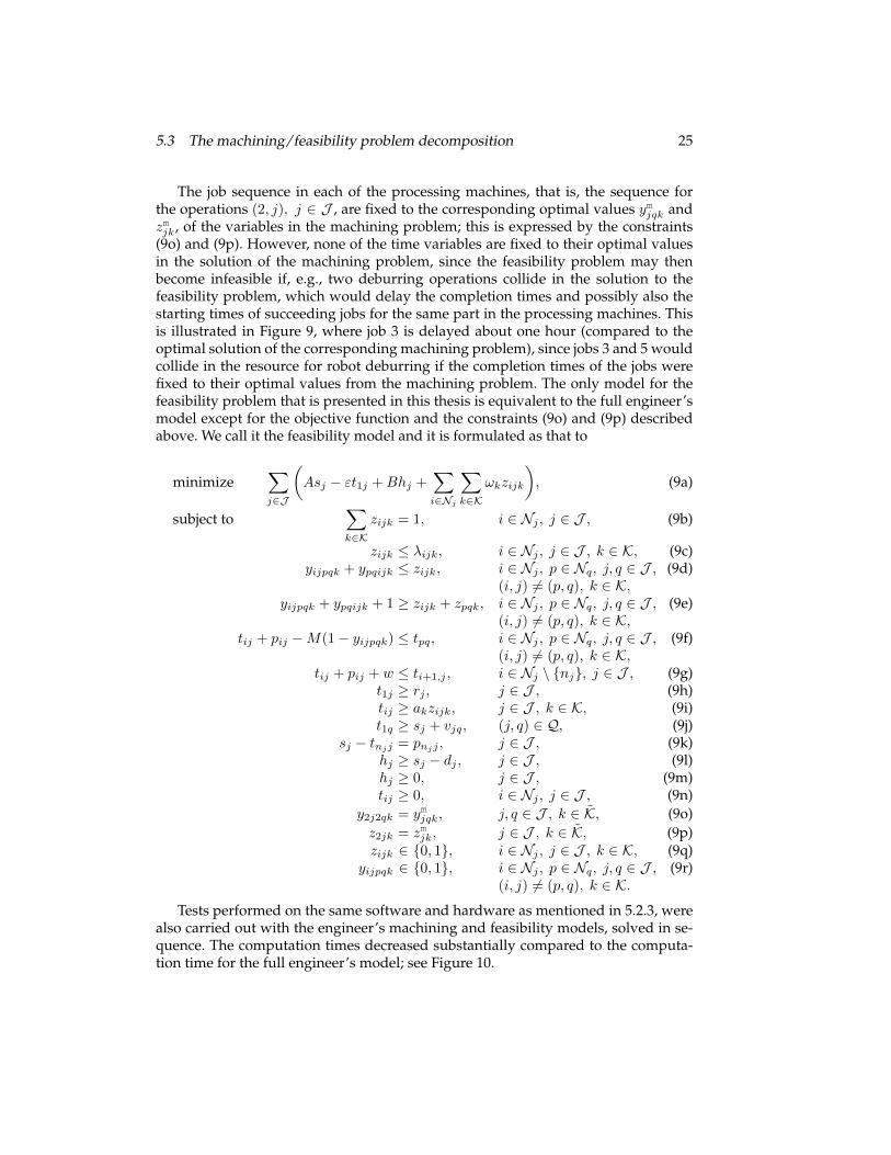
The job sequence in each of the processing machines, that is, the sequence forthe operations (2, j), j ∈ J , are fixed to the corresponding optimal values ymjqk andzmjk, of the variables in the machining problem; this is expressed by the constraints(9o) and (9p). However, none of the time variables are fixed to their optimal valuesin the solution of the machining problem, since the feasibility problem may thenbecome infeasible if, e.g., two deburring operations collide in the solution to thefeasibility problem, which would delay the completion times and possibly also thestarting times of succeeding jobs for the same part in the processing machines. Thisis illustrated in Figure 9, where job 3 is delayed about one hour (compared to theoptimal solution of the corresponding machining problem), since jobs 3 and 5 wouldcollide in the resource for robot deburring if the completion times of the jobs werefixed to their optimal values from the machining problem. The only model for thefeasibility problem that is presented in this thesis is equivalent to the full engineer’smodel except for the objective function and the constraints (9o) and (9p) describedabove. We call it the feasibility model and it is formulated as that to
minimize∑j∈J
(Asj − εt1j +Bhj +
∑i∈Nj
∑k∈K
ωkzijk
), (9a)
subject to∑k∈K
zijk = 1, i ∈ Nj , j ∈ J , (9b)
zijk ≤ λijk, i ∈ Nj , j ∈ J , k ∈ K, (9c)yijpqk + ypqijk ≤ zijk, i ∈ Nj , p ∈ Nq, j, q ∈ J , (9d)
(i, j) 6= (p, q), k ∈ K,yijpqk + ypqijk + 1 ≥ zijk + zpqk, i ∈ Nj , p ∈ Nq, j, q ∈ J , (9e)
(i, j) 6= (p, q), k ∈ K,tij + pij −M(1− yijpqk) ≤ tpq, i ∈ Nj , p ∈ Nq, j, q ∈ J , (9f)
(i, j) 6= (p, q), k ∈ K,tij + pij + w ≤ ti+1,j , i ∈ Nj \ {nj}, j ∈ J , (9g)
t1j ≥ rj , j ∈ J , (9h)tij ≥ akzijk, j ∈ J , k ∈ K, (9i)t1q ≥ sj + vjq, (j, q) ∈ Q, (9j)
sj − tnjj = pnjj , j ∈ J , (9k)hj ≥ sj − dj , j ∈ J , (9l)hj ≥ 0, j ∈ J , (9m)tij ≥ 0, i ∈ Nj , j ∈ J , (9n)
y2j2qk = ymjqk, j, q ∈ J , k ∈ K, (9o)z2jk = zmjk, j ∈ J , k ∈ K, (9p)zijk ∈ {0, 1}, i ∈ Nj , j ∈ J , k ∈ K, (9q)
yijpqk ∈ {0, 1}, i ∈ Nj , p ∈ Nq, j, q ∈ J , (9r)(i, j) 6= (p, q), k ∈ K.
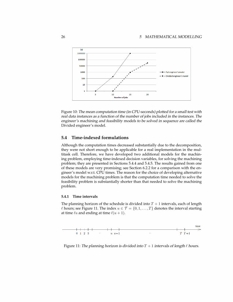
Tests performed on the same software and hardware as mentioned in 5.2.3, werealso carried out with the engineer’s machining and feasibility models, solved in se-quence. The computation times decreased substantially compared to the computa-tion time for the full engineer’s model; see Figure 10.
26 5 MATHEMATICAL MODELLING
Figure 10: The mean computation time (in CPU-seconds) plotted for a small test withreal data instances as a function of the number of jobs included in the instances. Theengineer’s machining and feasibility models to be solved in sequence are called theDivided engineer’s model.
5.4 Time-indexed formulations
Although the computation times decreased substantially due to the decomposition,they were not short enough to be applicable for a real implementation in the mul-titask cell. Therefore, we have developed two additional models for the machin-ing problem, employing time-indexed decision variables, for solving the machiningproblem; they are presented in Sections 5.4.4 and 5.4.5. The results gained from oneof these models are very promising; see Section 6.2.2 for a comparison with the en-gineer’s model w.r.t. CPU times. The reason for the choice of developing alternativemodels for the machining problem is that the computation time needed to solve thefeasibility problem is substantially shorter than that needed to solve the machiningproblem.
5.4.1 Time intervals
The planning horizon of the schedule is divided into T + 1 intervals, each of length` hours; see Figure 11. The index u ∈ T = {0, 1, . . . , T} denotes the interval startingat time `u and ending at time `(u+ 1).
Figure 11: The planning horizon is divided into T + 1 intervals of length ` hours.
5.4 Time-indexed formulations 27
The value of the parameter T has to be large enough such that the planning hori-zon of (T + 1)` hours contains an optimal schedule, but as small as possible, sincethe computation times become shorter for smaller values of T . The reason for this isexplained in Section 5.4.7, where a heuristic for determining a suitable value of T ispresented.
5.4.2 Definition of variables
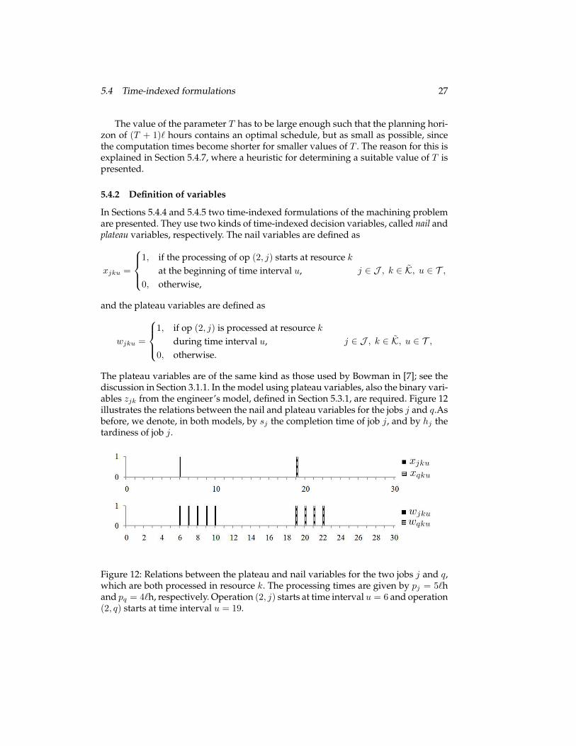
In Sections 5.4.4 and 5.4.5 two time-indexed formulations of the machining problemare presented. They use two kinds of time-indexed decision variables, called nail andplateau variables, respectively. The nail variables are defined as
xjku =
1, if the processing of op (2, j) starts at resource k
at the beginning of time interval u,0, otherwise,
j ∈ J , k ∈ K, u ∈ T ,
and the plateau variables are defined as
wjku =
1, if op (2, j) is processed at resource k
during time interval u,0, otherwise.
j ∈ J , k ∈ K, u ∈ T ,
The plateau variables are of the same kind as those used by Bowman in [7]; see thediscussion in Section 3.1.1. In the model using plateau variables, also the binary vari-ables zjk from the engineer’s model, defined in Section 5.3.1, are required. Figure 12illustrates the relations between the nail and plateau variables for the jobs j and q.Asbefore, we denote, in both models, by sj the completion time of job j, and by hj thetardiness of job j.
Figure 12: Relations between the plateau and nail variables for the two jobs j and q,which are both processed in resource k. The processing times are given by pj = 5`hand pq = 4`h, respectively. Operation (2, j) starts at time interval u = 6 and operation(2, q) starts at time interval u = 19.
28 5 MATHEMATICAL MODELLING
5.4.3 New values for all time parameters
All parameters related to time used in the time-indexed models have to be expressedas multiples of time periods. In order to maintain the feasibility of every solutionto the resulting model, this means that the values of pj , ak, and rmj must be scaledand rounded up, while the due dates, dj , have to be scaled and truncated. Newparameters are thus defined according to
pj :=⌈pj`
⌉, rmj :=
⌈rmj`
⌉, and dj :=
⌊dj`
⌋, j ∈ J ,
ak :=⌈ak`
⌉, k ∈ K.
Regarding jobs to be performed on the same physical part, say (j, q) ∈ Q, the param-eter vmjq is redefined to represent the planned lead time between the start of operation(2, j) and the start of operation (2, q) according to
vpmjq :=
⌈1
`(pj + ppmj + vmjq)
⌉, (j, q) ∈ Q.
The parameter ppmj is analogously redefined to include the processing time of themachining operation, before it is scaled and rounded up, as
ppmj :=
⌈1
`(pj + ppmj )
⌉, j ∈ J .
5.4.4 A time-indexed model with nail variables
The time-indexed model with so-called nail variables presented in this section hasbeen developed using findings presented in [60]. We also present an alternative for-mulation of the constraints (11e).
The model is to
minimize∑j∈J
(Asj +Bhj), (11a)
subject to∑k∈K
∑u∈T
xjku = 1, j ∈ J , (11b)
∑u∈T
xjku≤λjk, j ∈ J , k∈K, (11c)
∑j∈J
u∑ν=(u−pj+1)+
xjkν≤ 1, k ∈ K, u = 0, . . . , T, (11d)
∑k∈K
u∑µ=0
xjkµ −u+vpmjq∑ν=0
xqkν
≥ 0, (j, q) ∈ Q, u = 0, . . . , T − vpmjq , (11e)
5.4 Time-indexed formulations 29
xjku = 0, (j, q) ∈ Q, k ∈ K, u = T − vpmjq , . . . , T, (11f)∑k∈K
∑u∈T
uxjku + ppmj = sj , j ∈ J , (11g)
sj − hj ≤ dj , j ∈ J , (11h)
hj ≥ 0, j ∈ J , (11i)
xjku = 0, j ∈ J , k ∈ K, u = 0, . . . ,max{rmj ; ak}, (11j)
xjku ∈ {0,1}, j ∈ J , k ∈ K, u ∈ T , (11k)
where (u)+ := max{0;u} denotes the projection of u ∈ Z onto Z+. The model withnail variables is equivalent to the engineer’s model (7) in Section 5.3.1 for the casewhen all data in the latter are given in entire time intervals, i.e., expressed in multi-ples of `.
The variables zjk, tj , and yjqk of the engineer’s model are related to the time-indexed model’s nail variables xjku as follows:
zjk =∑u∈T
xjku, j ∈ J , k ∈ K, (12a)
tj =∑k∈K
∑u∈T
uxjku, j ∈ J , (12b)
yjqk =
1, if 0 <∑u∈T
uxjku <∑u∈T
uxqku,
0, otherwise,j, q ∈ J , j 6= q, k ∈ K. (12c)
Conversely, the time-indexed model’s variables can be expressed in terms of thevariables of the engineer’s model (provided that all data are given in multiples ofthe length ` of the time intervals)
xjku =
{zjk, u = tj ,
0, u ∈ T \ {tj},j ∈ J , k ∈ K. (13)
The constraints (11b) ensure that every operation (2, j) is processed exactly once,and the constraints (11c) make sure that each machining operation is scheduled inan allowed resource. These constraints are, through the equivalences (12) and (13),equivalent to the constraints (7b) and (7c) of the engineer’s model, respectively. Theconstraints (11d), which regulate that only one operation at a time is scheduled inresource k, correspond to the constraints (7d)–(7f).
The constraints (11e)–(11f) ensure that operation (2, j) is scheduled to start atleast the planned lead time of vpmjq time steps before the start of operation (2, q), for allindices j, q ∈ J such that (j, q) ∈ Q. These constraints correspond to the constraints(7i) of the engineer’s model. We have also developed the following set of constraintswhich equivalently describe these precedence relations:
∑k∈K
T∑µ=u
xjkµ +
u+vpmjq−1∑ν=0
xqkν
≤ 1, (j, q) ∈ Q, u = 0, . . . , T − vpmjq + 1. (14)

30 5 MATHEMATICAL MODELLING
Preliminary computational tests indicate that the constraints (14) are as strong as theconstraints (11e). A closer study of the differences between these constraints is aninteresting subject for further research.
The constraints (11g)–(11i) define the completion times, sj and the tardiness, hj ,as do the constraints (7j)–(7l). The constraints (11j) make sure that operation (2, j) isnot scheduled before its release date or before the resource k chosen by the model isavailable, and correspond to the constraints (7g) and (7h) of the engineer’s model.
5.4.5 A time-indexed model with plateau variables
Compared with using the nail variables or those in the engineer’s model (7), oneadvantage gained by using the plateau variables wjku, as defined in Section 5.4.2,is that it is easy to employ the objective function described in Section 5.4.6, i.e., tominimize the work load variance. The model with the plateau variables is, however,a weaker formulation than the model (11), since the plateau variables are aggregatesof nail variables; see the equations (16) below and the discussion that follows. (Foran illustrative example of weak and strong formulations related to variable aggre-gations, see [61, Section 13.4.1].) Moreover, preliminary tests show that the time-indexed model with plateau variables requires longer computation times for solvingour test instances of the scheduling problem, than the model (11).
The model is to
minimize∑j∈J
(Asj +Bhj), (15a)
subject to∑k∈K
zjk = 1, j ∈ J , (15b)
zjk ≤λjk, j ∈ J , k ∈ K, (15c)
wjku + wqku≤ 1, j, q ∈ J , j 6= q, k ∈ K, u ∈ T , (15d)
wjku≤ zjk, j ∈ J , k ∈ K, u ∈ T , (15e)∑k∈K
∑u∈T
wjku = pj , j ∈ J , (15f)
∑k∈K
(pjwjku− pjwjk,u+1 +
T∑ν=u+2
wjkν
)≤ pj , j ∈ J , u = 0, . . . , T − 2, (15g)
∑k∈K
(wjku + wjk,u+1 +
T∑ν=u+vpmjq
wqkν
)≤ pq+1, (j, q) ∈ Q, u = 0, . . . , T−vpmjq , (15h)
∑k∈K
rj∑u=0
wjku = 0, j ∈ J , (15i)
∑j∈J
ak∑u=0
wjku = 0, k ∈ K, (15j)
5.4 Time-indexed formulations 31
u∑k∈K
(wjk,u−1 − wjku)≤ sj , j ∈ J , u = 1, . . . , T, (15k)
hj ≥ sj− dj , j ∈ J , (15l)hj ≥ 0, j ∈ J , (15m)sj ≥ 0, j ∈ J , (15n)
wjku ∈ {0, 1}, j ∈ J , k ∈ K, u ∈ T , (15o)zjk ∈ {0, 1}, j ∈ J , k ∈ K. (15p)
The plateau variables wjku are related to the time-indexed model’s nail variablesxjku as follows:
wjku =
u∑ν=(u−pj+1)+
xjkν , j ∈ J , k ∈ K, u ∈ T . (16)
The variables wjku are hence positive linear combinations of the nail variables. Theallocation variables, zjk, are given by (12a) in the previous section.
Conversely, the nail variables can be expressed in terms of the plateau variablesas
xjku =
{max{0, wjku − wj,k,u−1}, u = 1, . . . , T,
wjku, u = 0,j ∈ J , k ∈ K. (17)
Like the constraints (11b) and (11c), the constraints (15b) and (15c) ensure that ev-ery machining operation is processed exactly once, and that each operation is sched-uled on an allowed resource. The constraints (15d) make sure that no two operations(2, j) and (2, q) are simultaneously scheduled in the same resource, as do the con-straints (11d) in the time-indexed model with nail variables. The constraints (15e)relate the plateau variables wjku to the allocation variables zjk, so that wjku = 0 forall resources k but the one chosen for the job j, i.e., the resource for which zjk = 1.The constraints (15f)–(15g) ensure that there are exactly pj 1-valued plateau vari-ables and that these appear consecutively along the time axis. The constraints (15h),which correspond to the constraints (11e), separate the machining operations of thejobs j and q, where (j, q) ∈ Q, by the planned interoperation time vpmjq . Analogouslyto the constraints (11j), the constraints (15i) and (15j) ensure, respectively, that nomachining operation is scheduled before its release date or in a resource that is notavailable.
The value of (wjk,u−1 − wjku) in the constraints (15k) equals −1 when u is thestarting time of operation (2, j); it equals 1 when u is the operation’s completiontime. Therefore, the completion time sj cannot be defined by using an equality incontrast to the models (7) and (11). Denote by tj and sj the values of the starting andcompletion times, respectively, of a job j in an optimal solution. Using the optimalvalues of the plateau variables, the left hand side of (15k) then equals −tj and sj foru = tj and sj , respectively; it equals 0 for u ∈ T \ {tj , sj}. Hence, the largest value ofany left hand side of (15k) will always be equal to the completion time of job j. Sincethe minimization of the sum of the completion times is part of the objective function(15a), the variables sj will attain their respective correct values.
32 5 MATHEMATICAL MODELLING
5.4.6 Minimizing work load variance
There are many views of what defines a good schedule, and one has to analyze thecurrent logistic environment in order to determine what suits best the current situa-tion. The objective functions presented in the preceding formulations of the schedul-ing problem focus on scheduling the jobs as soon as they are available and on mini-mizing the total tardiness. This way the lead times within the cell are minimized. Butsince the processing in the multitask cell is a part of the whole production process,the total lead time of the parts processed in the cell will probably not decrease muchif some parts are produced too early, due to the objective of minimizing total com-pletion times and total tardiness in the multitask cell. Another disadvantage of thisobjective function is that it produces schedules in which short jobs are typically pro-cessed before longer jobs. This is in fact the property of the well known dispatchingrule shortest-processing-time (SPT) (of the theory of production logistics) mentionedin Section 3.2. However, if parts of the same type arrive in clusters to the next opera-tion (e.g. the operation µmj+1 being the operation to be performed directly after jobj in Figure 8), there is a risk for long queues before this operation which may resultin longer total lead times for the product.
One alternative to the objective of minimizing the sum of completion times andtotal tardiness is to produce a schedule in which the instant work load being as closeto a target work load as possible, while the objective term of weighted total tardi-ness is retained. Hence, the objective will be to minimize the weighted sum of thesum of the absolute differences between the actual work load and the target workload in each time step of the main planning period and the total tardiness. With theplateau variable wjku, whose value equals 1 if resource k is occupied by job j duringtime interval u, a linear approximation of the work load in the multitask cell can beformulated. The time-indexed model with nail variables can also be used with thisobjective, replacing wjku below by the expression given in (16).
The work load per time unit during time interval u of length ` is given by theexpression `−1
∑j∈J
∑k∈K wjku. Letting the target work load per time unit for the
planning period be denoted by btargetu , the objective function can be expressed asthat to
minimize AT plan∑u=0
∣∣∣∣∣∣1`∑j∈J
∑k∈K
wjku − btargetu
∣∣∣∣∣∣+B∑j∈J
hj , (18)
where T plan ≤ T is the end of the main planning period; the value of T plan is lessthan the value of T , since the planning horizon T must allow all jobs to be scheduled,and hence there needs to be a period with declining work load towards the end ofthe total planning period; see Figure 13.
In the example schedule in Figure 14, the length of the planning horizon is T = 70and a suitable choice for the length of the main planning period is T plan = 40, sincethere is a decline in the work load after this point in time.
In order to retain a linear objective function, we introduce the two continuousnon-negative variables b−u and b+u ; their sum is defined to equal the absolute differ-ence between the instant work load and the target work load in time interval u. The
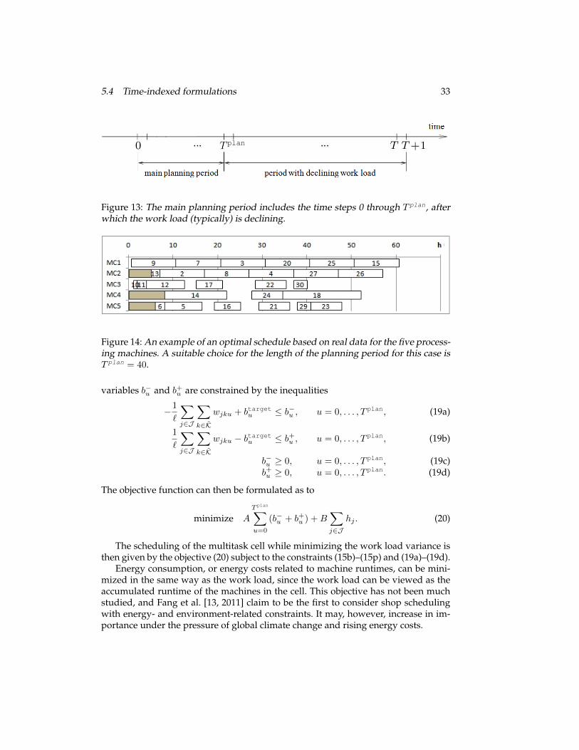
5.4 Time-indexed formulations 33
Figure 13: The main planning period includes the time steps 0 through T plan, afterwhich the work load (typically) is declining.
Figure 14: An example of an optimal schedule based on real data for the five process-ing machines. A suitable choice for the length of the planning period for this case isT plan = 40.
variables b−u and b+u are constrained by the inequalities
−1
`
∑j∈J
∑k∈K
wjku + btargetu ≤ b−u , u = 0, . . . , T plan, (19a)
1
`
∑j∈J
∑k∈K
wjku − btargetu ≤ b+u , u = 0, . . . , T plan, (19b)
b−u ≥ 0, u = 0, . . . , T plan, (19c)b+u ≥ 0, u = 0, . . . , T plan. (19d)
The objective function can then be formulated as to
minimize A
T plan∑u=0
(b−u + b+u ) +B∑j∈J
hj . (20)
The scheduling of the multitask cell while minimizing the work load variance isthen given by the objective (20) subject to the constraints (15b)–(15p) and (19a)–(19d).
Energy consumption, or energy costs related to machine runtimes, can be mini-mized in the same way as the work load, since the work load can be viewed as theaccumulated runtime of the machines in the cell. This objective has not been muchstudied, and Fang et al. [13, 2011] claim to be the first to consider shop schedulingwith energy- and environment-related constraints. It may, however, increase in im-portance under the pressure of global climate change and rising energy costs.
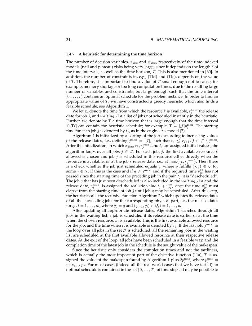
34 5 MATHEMATICAL MODELLING
5.4.7 A heuristic for determining the time horizon
The number of decision variables, xjku and wjku, respectively, of the time-indexedmodels (nail and plateau) risks being very large, since it depends on the length ` ofthe time intervals, as well as the time horizon, T . This is also mentioned in [60]. Inaddition, the number of constraints in, e.g., (11d) and (11e), depends on the valueof T . Therefore, it is important to find a value of T small enough not to cause, forexample, memory shortage or too long computation times, due to the resulting largenumber of variables and constraints, but large enough such that the time interval[0, . . . , T ] contains an optimal schedule for the problem instance. In order to find anappropriate value of T , we have constructed a greedy heuristic which also finds afeasible schedule; see Algorithm 1.
We let τk denote the time from which the resource k is available, rheurj the releasedate for job j, and waiting_list a list of jobs not scheduled instantly in the heuristic.Further, we denote by T a time horizon that is large enough that the time interval[0,T`] can contain the heuristic schedule; for example, T = |J |pmax
j . The startingtime for each job j is denoted by tj , as in the engineer’s model (7).
Algorithm 1 is initialized by a sorting of the jobs according to increasing valuesof the release dates, i.e., defining jmax = |J |, such that rj ≤ rj+1, j ∈ J \ jmax.After the initialization, in which xjku, τk, rheurj , and tj are assigned initial values, thealgorithm loops over all jobs j ∈ J . For each job, j, the first available resource kallowed is chosen and job j is scheduled in this resource either directly when theresource is available, or at the job’s release date, i.e., at max{τk, rheurj }. Then thereis a check whether the job just scheduled equals q, where q fulfills (, q) ∈ Q forsome ∈ J . If this is the case and if q 6= jmax, and if the required time vpmq has notpassed since the starting time of the preceding job in the pair, t, it is ”descheduled”.The job q that has just been descheduled is also included in the waiting_list and therelease date, rheurq , is assigned the realistic value t + vpmq , since the time vpmq mustelapse from the starting time of job until job q may be scheduled. After this step,the heuristic calls the recursive function Algorithm 2 which updates the release datesof all the succeeding jobs for the corresponding physical part, i.e., the release datesfor qi, i = 1, . . . ,m, where q0 = q and (qi−1, qi) ∈ Q, i = 1, . . . ,m.
After updating all appropriate release dates, Algorithm 1 searches through alljobs in the waiting list; a job is scheduled if its release date is earlier or at the timewhen the chosen resource, k, is available. This is the first available allowed resourcefor the job, and the time when it is available is denoted by τk. If the last job, jmax, inthe loop over all jobs in the set J is scheduled, all the remaining jobs in the waitinglist are scheduled at the first available allowed resource at their respective releasedates. At the exit of the loop, all jobs have been scheduled in a feasible way, and thecompletion time of the latest job in the schedule is the sought value of the makespan.
Since the heuristic only considers the completion times and not the tardiness,which is actually the most important part of the objective function (11a), T is as-signed the value of the makespan found by Algorithm 1 plus 2pmax
j , where pmaxj =
maxj∈J pj . For most cases (indeed all the real-world cases that we have tested) anoptimal schedule is contained in the set {0, . . . , T} of time steps. It may be possible to
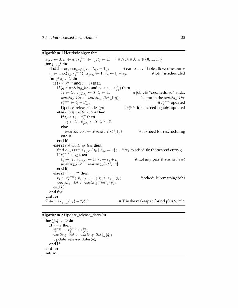
5.4 Time-indexed formulations 35
Algorithm 1 Heuristic algorithm
xjku ← 0, τk ← ak, rheurj ← rj , tj ← T, j ∈ J , k ∈ K, u ∈ {0, ...,T; }
for j ∈ J dofind k ∈ argmink∈K { τk | λjk = 1 }; # earliest available allowed resourcetj ← max{τk; rheurj }; xjktj ← 1; τk ← tj + pj ; # job j is scheduledfor (, q) ∈ Q do
if (j 6= jmax and j = q) thenif (q /∈ waiting_list and tq < t + vpmq ) thenτk ← tq; xq,k,tq ← 0; tq ← T; # job q is ”descheduled” and...waiting_list← waiting_list
⋃{q}; # ...put in the waiting_list
rheurq ← t + vpmq ; # rheurj updatedUpdate_release_dates(q); # rheurq for succeeding jobs updated
else if q ∈ waiting_list thenif tq < t + vpmq thenτk ← tq; xqktq ← 0; tq ← T;
elsewaiting_list← waiting_list \ {q}; # no need for rescheduling
end ifend if
else if q ∈ waiting_list thenfind k ∈ argmink∈K { τk | λqk = 1 }; # try to schedule the second entry q...if rheurq ≤ τk thentq ← τk; xq,k,tq ← 1; τk ← tq + pq; # ...of any pair ∈ waiting_listwaiting_list← waiting_list \ {q};
end ifelse if j = jmax thentq ← rheurq ; xq,k,tq ← 1; τk ← tq + pq; # schedule remaining jobswaiting_list← waiting_list \ {q};
end ifend for
end forT ← maxk∈K{τk}+ 2pmax
j # T is the makespan found plus 2pmaxj .
Algorithm 2 Update_release_dates(q)for (, q) ∈ Q do
if = q thenrheurq ← rheur + vpmq ;waiting_list← waiting_list
⋃{q};
Update_release_dates(q);end if
end forreturn
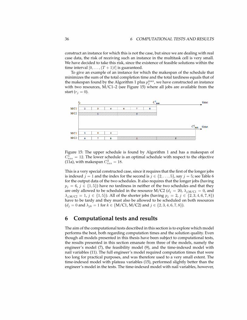
36 6 COMPUTATIONAL TESTS AND RESULTS
construct an instance for which this is not the case, but since we are dealing with realcase data, the risk of receiving such an instance in the multitask cell is very small.We have decided to take this risk, since the existence of feasible solutions within thetime interval [0, . . . , (T + 1)`] is guaranteed.
To give an example of an instance for which the makespan of the schedule thatminimizes the sum of the total completion time and the total tardiness equals that ofthe makespan found by the Algorithm 1 plus pmax
j , we have constructed an instancewith two resources, M/C1–2 (see Figure 15) where all jobs are available from thestart (rj = 0).
Figure 15: The upper schedule is found by Algorithm 1 and has a makespan ofC1max = 12. The lower schedule is an optimal schedule with respect to the objective
(11a), with makespan C2max = 18.
This is a very special constructed case, since it requires that the first of the longer jobsis indexed j = 1 and the index for the second is j ∈ {2, . . . , 5}, say j = 5; see Table 6for the output data of the two schedules. It also requires that the longer jobs (havingpj = 6, j ∈ {1, 5}) have no tardiness in neither of the two schedules and that theyare only allowed to be scheduled in the resource M/C2 (dj = 20, λj,M/C1 = 0, andλj,M/C2 = 1, j ∈ {1, 5}). All of the shorter jobs (having pj = 2, j ∈ {2, 3, 4, 6, 7, 8})have to be tardy and they must also be allowed to be scheduled on both resources(dj = 0 and λjk = 1 for k ∈ {M/C1, M/C2} and j ∈ {2, 3, 4, 6, 7, 8}).
6 Computational tests and results
The aim of the computational tests described in this section is to explore which modelperforms the best, both regarding computation times and the solution quality. Eventhough all models presented in this thesis have been subject to computational tests,the results presented in this section emanate from three of the models, namely theengineer’s model (7), the feasibility model (9), and the time-indexed model withnail variables (11). The full engineer’s model required computation times that weretoo long for practical purposes, and was therefore used to a very small extent. Thetime-indexed model with plateau variables (15), performed slightly better than theengineer’s model in the tests. The time-indexed model with nail variables, however,

6.1 Test data 37
Schedule found by Algorithm 1 Optimal schedulej k sj hj sj + hj k sj hj sj + hj1 M/C2 6 0 6 M/C2 12 0 122 M/C1 2 2 4 M/C1 2 2 43 M/C1 4 4 8 M/C1 4 4 84 M/C1 6 6 12 M/C1 6 6 125 M/C2 12 0 12 M/C2 18 0 186 M/C1 8 8 16 M/C2 2 2 47 M/C1 10 10 20 M/C2 4 4 88 M/C1 12 12 24 M/C2 6 6 12∑8j=1 60 42 102 54 24 78
Table 6: Data describing the schedules illustrated in Figure 15.
outperformed the model (15) (with plateau variables), therefore, the latter model wasnot further investigated.
The computational results are given for the models (7) and (11) for real data in-stances collected from the ERP system at Volvo Aero in the year of 2010. The compu-tations regarding the comparisons with the dispatching rules in Section 6.2.3 werecarried out on a 4Gb quad-core Intel Xeon 3.2 GHz system using AMPL-CPLEX12 asoptimization software. All other computations have been carried out using AMPL-CPLEX12 on a computer with two 2.66GHz Intel Xeon 5650, each having six cores(24 threads); its total memory was 48Gbyte RAM.
6.1 Test data
All data used in all tests described in this section originate from real production in-stances in the multitask cell. One of the problems encountered due to the choice ofusing real data is that planned orders that have not yet been started according tothe plan may be present in the system. Then, the release dates of all planned ordersrelated to the same product that are currently delayed (calculated by the formula (1)given in Section 5.1.4) will have the same value, namely that of ν0
j , i.e., the plannedlead time—illustrated in Figure 8—from the release of the order into the productionuntil its arrival to the multitask cell. It is, however, not plausible that all plannedorders that are currently delayed, will be released at time t0; hence, these orders—ifthey exist—have to be (manually) assigned plausible release dates before the calcu-lation of an optimal schedule is made in an implementation. Such plausible releasedates have not been set for the instances used for obtaining the results given in thissection, and hence some jobs of the same kind may share release dates.

38 6 COMPUTATIONAL TESTS AND RESULTS
6.2 Validation and tests
As mentioned in Section 5.1.5 it is important that the value of the weight ε in theobjective function (9a) chosen for the feasibility problem is much smaller than thoseof A and B. We have chosen the values A = B = 1 and ε = 0.001 in all the compu-tations presented in this section. The choice of having A = B = 1 was made sincethe two goals, short completion times and low tardiness, are not contradictory. How-ever, when studying some test results, we discovered some cases where jobs with notardiness, but short processing times, were scheduled in clusters before longer tardyjobs. This indicates that the choice of A = B was unfortunate; finding appropriatevalues of these weights is an area of future study.
The influence of the size of the discretization interval ` for the time-indexedmodel (11) with nail variables on the solution quality and the computation timesis described in Sections 6.2.1 and 6.2.2, respectively. In these sections, results fromthe engineer’s model are also given. In Section 6.2.3, the results from the applicationof the model (11) are compared with schedules resulting from the use of dispatchingrules, and in Section 6.2.4, the influence on computation times of the choice of thevalue for the parameter M for the engineer’s model is discussed. A summary of theresults is given in Section 7.
6.2.1 Estimated error due to the choice of ` for the time-indexed models
The starting and completion times obtained from the optimal solutions to the time-indexed model (11) with nail variables, are given in terms of multiples of the length` of the time discretization interval. Therefore, the optimal objective value of (11)differs from that of the engineer’s model (7). Thus the completion times sj are re-calculated using the original (i.e., non-discrete) data, while retaining the ordering ofthe operations on each of the processing machines received from the solution to themodel (11). For the example illustrated in Figure 16, the discrete release date of job4 is 18h, while the real release date is 17.5h, which is the reason for the idle periodbetween jobs 2 and 4 in the schedule. The value of the solution obtained after thispost-processing can then be compared with the optimal value from the engineer’smodel (7). This post-processing of data required at most 0.04s of computation timefor each of the six scenarios constructed from the data set described below, compris-ing 70 jobs.
Figure 16: The output of the discrete time machining model is post-processed usingthe original non-discrete data.

6.2 Validation and tests 39
Results from the engineer’s model and the time-indexed model with differentvalues of ` have been compared for six real scenarios collected from the multitask cellduring the autumn of 2010. For each scenario, the jobs were initially sorted accordingto increasing values of the release dates, rj . Different test instances were then createdby selecting the first 5m jobs in the queue of jobs, where m ∈ {1, . . . , 14}, such thatthe smallest and largest instances comprise 5 and 70 jobs, respectively.
A limit of 7200s was set for the computation time (clocktime), since 2h is in theupper limit of what could be accepted in practice. Fortunately, only a few of thelarger instances required such long computation times, at least in the tests performedwith the time-indexed model with nail variables. The limit of 7200s was, however,reached when using the engineer’s model; the calculations were then disrupted forsome scenarios with 20 jobs, and no optimal solutions were obtained for any scenariowith |J | ≥ 25. The time-indexed model performed, however, better and we obtainedoptimal solutions for all instances with |J | ≤ 60 and ` ≥ 1h before the time limit wasreached; see Section 6.2.2 for details on these computations.
In Table 7, the mean values of the relative differences between the optimal valuesfrom different models are listed. Since optimal values were only obtained for all sce-narios with |J | ≤ 15 when using the engineer’s model, it was solely compared to theresult from the time-indexed model with ` = 0.25h; results are missing for |J | ≥ 20.The optimal values obtained using the engineer’s model were identical with thoseobtained using model (11) for all instances with 10 and 15 jobs. All the other optimalsolutions found by the time-indexed model with ` > 0.25h were compared to thosefound by this model with ` = 0.25h.
Diff to (7) Diff to (11) Diff to (11) Diff to (11)# jobs ` = 0.25h ` = 0.5h ` = 1h ` = 2h
10 0.000 0.000 0.000 0.03115 0.000 0.005 0.010 0.08320 – 0.001 0.018 0.06125 – 0.015 0.02830 – 0.015 0.034 0.11235 – 0.019 0.02240 – 0.022 0.027 0.17245 – 0.022 0.02550 – 0.028 0.035 0.335
Mean 0.000 0.014 0.022 0.132
Table 7: Mean differences between the optimal values from different models. Thetime-indexed model (11) with ` = 0.25h is compared with the engineer’s model (7),while the time-indexed model with ` > 0.25h is compared with the same modelwith ` = 0.25h. The differences are given in percent with regard to the optimal valuefrom the model compared. The notation – means that the corresponding results aremissing.
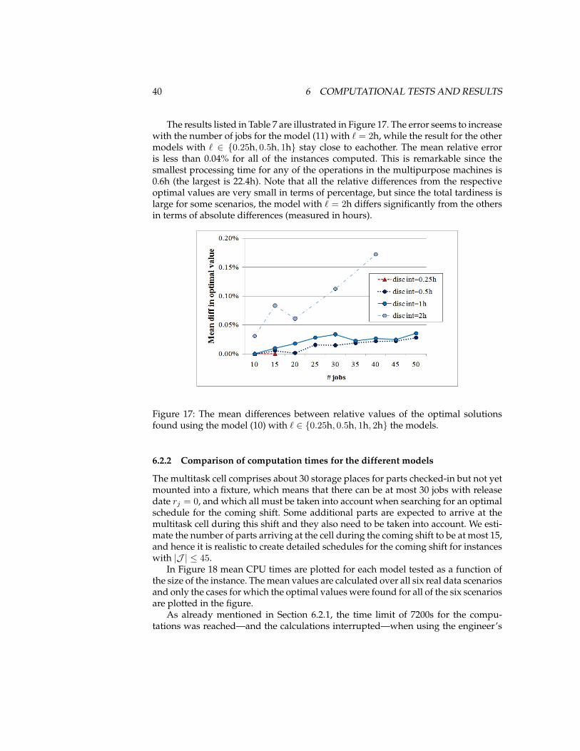
40 6 COMPUTATIONAL TESTS AND RESULTS
The results listed in Table 7 are illustrated in Figure 17. The error seems to increasewith the number of jobs for the model (11) with ` = 2h, while the result for the othermodels with ` ∈ {0.25h, 0.5h, 1h} stay close to eachother. The mean relative erroris less than 0.04% for all of the instances computed. This is remarkable since thesmallest processing time for any of the operations in the multipurpose machines is0.6h (the largest is 22.4h). Note that all the relative differences from the respectiveoptimal values are very small in terms of percentage, but since the total tardiness islarge for some scenarios, the model with ` = 2h differs significantly from the othersin terms of absolute differences (measured in hours).
Figure 17: The mean differences between relative values of the optimal solutionsfound using the model (10) with ` ∈ {0.25h, 0.5h, 1h, 2h} the models.
6.2.2 Comparison of computation times for the different models
The multitask cell comprises about 30 storage places for parts checked-in but not yetmounted into a fixture, which means that there can be at most 30 jobs with releasedate rj = 0, and which all must be taken into account when searching for an optimalschedule for the coming shift. Some additional parts are expected to arrive at themultitask cell during this shift and they also need to be taken into account. We esti-mate the number of parts arriving at the cell during the coming shift to be at most 15,and hence it is realistic to create detailed schedules for the coming shift for instanceswith |J | ≤ 45.
In Figure 18 mean CPU times are plotted for each model tested as a function ofthe size of the instance. The mean values are calculated over all six real data scenariosand only the cases for which the optimal values were found for all of the six scenariosare plotted in the figure.
As already mentioned in Section 6.2.1, the time limit of 7200s for the compu-tations was reached—and the calculations interrupted—when using the engineer’s

6.2 Validation and tests 41
Figure 18: Mean CPU times plotted for the engineer’s model (7) (eng) and the time-indexed model (11) with nail variables for different values ` of the discretizationinterval. The instances computed are represented by the markers in the graph. Themean values are calculated over six real data instances.
model (7) for solving some scenarios with 20 jobs. The time-indexed model (11) withnail variables performed better; see Figure 18. We verify, for all of the instances buttwo, the anticipated relation that the computation times grow with a decreasingvalue of `. The model (11) with ` = 0.5h had trouble finding an optimal solutionfor one scenario with |J | ≥ 45. Hence, one should choose the value of ` as large aspossible in order to possess short computation times, but also as small as possiblein order to get solutions of good quality. From Section 6.2.1 we know that the differ-ences in optimal values between the model (11) with ` = 1h and ` = 0.25h were verysmall for the test set. Hence ` = 1h seems to be a good choice for the value of thisparameter.
The model (11) with ` = 1h required on average 40 CPU-seconds to find an op-timal solution for scenarios with 45 jobs, which we have estimated to be the largestsize of a realistic instance for computing an optimal schedule for the coming shift.This model succeeded in finding an optimal schedule for two out of the six scenar-ios with |J | = 70, one within only 18.5 CPU-seconds, and the other within 16832.3CPU-seconds (20 minutes of clocktime). The other instances were disrupted after7200 seconds (clocktime), where the maximum relative mipgap (the maximum rel-ative difference between the objective function found and the optimal value) was0.055%.
Although the model (11) with ` = 2h was shown to yield a bigger error than did
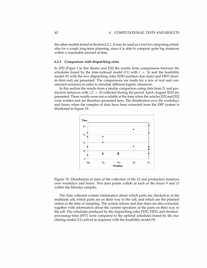
42 6 COMPUTATIONAL TESTS AND RESULTS
the other models tested in Section 6.2.1, it may be used as a tool for computing sched-ules for a rough long-term planning, since it is able to compute quite big instanceswithin a reasonable amount of time.
6.2.3 Comparison with dispatching rules
In [55] (Paper I in this thesis) and [52] the results from comparisons between theschedules found by the time-indexed model (11) with ` = 1h and the feasibilitymodel (9) with the two dispatching rules EDD (earliest–due–date) and FIFO (first–in–first–out) are presented. The comparisons are made for a mix of real and con-structed scenarios in order to simulate different logistic situations.
In this section the results from a similar comparison using data from 21 real pro-duction instances with |J | = 20 collected during the period April–August 2010 arepresented. These results were not available at the time when the articles [55] and [52]were written and are therefore presented here. The distribution over the weekdaysand hours when the samples of data have been extracted from the ERP system isillustrated in Figure 19.
Figure 19: Distribution in time of the collection of the 21 real production instancesover weekdays and hours. Two data points collide at each of the hours 9 and 11within the Monday samples.
The data collected contain information about which parts are checked-in at themultitask cell, which parts are on their way to the cell, and which are the plannedorders at the time of sampling. The system release and due dates are also extracted,together with information about the current operation of the parts on their way tothe cell. The schedules produced by the dispatching rules EDD, FIFO, and shortest–processing–time (SPT) were compared to the optimal schedules found by the ma-chining model (11) solved in sequence with the feasibility model (9).
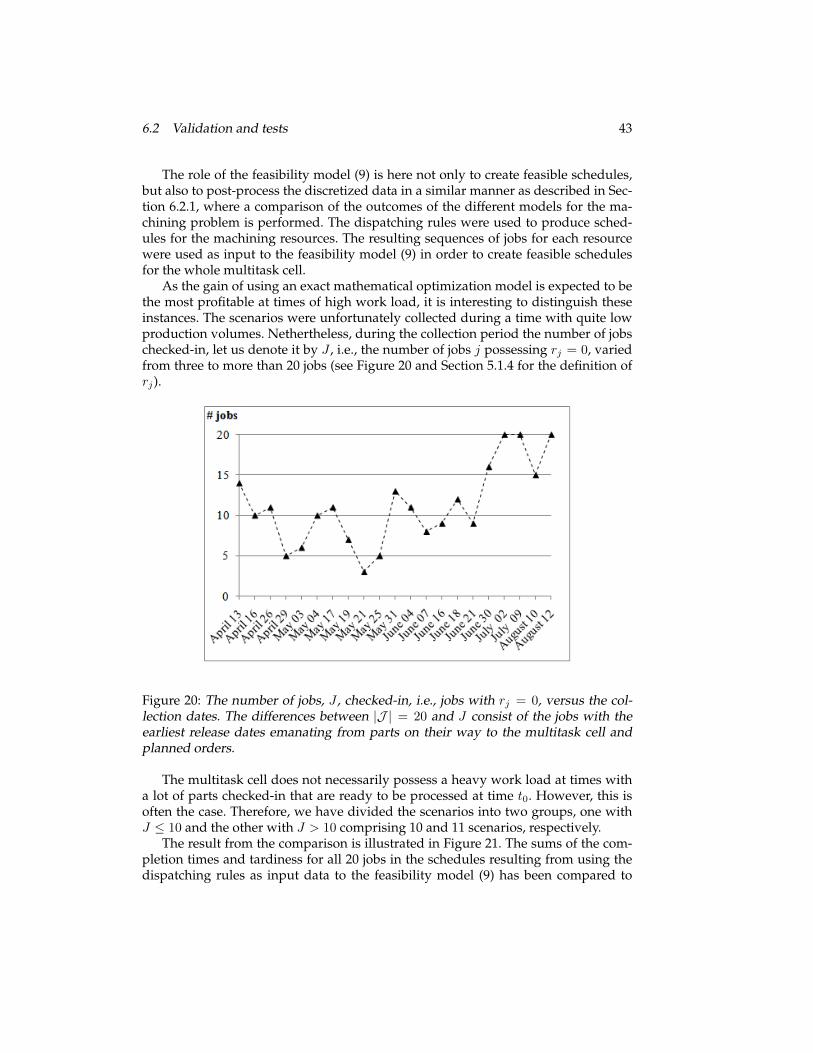
6.2 Validation and tests 43
The role of the feasibility model (9) is here not only to create feasible schedules,but also to post-process the discretized data in a similar manner as described in Sec-tion 6.2.1, where a comparison of the outcomes of the different models for the ma-chining problem is performed. The dispatching rules were used to produce sched-ules for the machining resources. The resulting sequences of jobs for each resourcewere used as input to the feasibility model (9) in order to create feasible schedulesfor the whole multitask cell.
As the gain of using an exact mathematical optimization model is expected to bethe most profitable at times of high work load, it is interesting to distinguish theseinstances. The scenarios were unfortunately collected during a time with quite lowproduction volumes. Nethertheless, during the collection period the number of jobschecked-in, let us denote it by J , i.e., the number of jobs j possessing rj = 0, variedfrom three to more than 20 jobs (see Figure 20 and Section 5.1.4 for the definition ofrj).
Figure 20: The number of jobs, J , checked-in, i.e., jobs with rj = 0, versus the col-lection dates. The differences between |J | = 20 and J consist of the jobs with theearliest release dates emanating from parts on their way to the multitask cell andplanned orders.
The multitask cell does not necessarily possess a heavy work load at times witha lot of parts checked-in that are ready to be processed at time t0. However, this isoften the case. Therefore, we have divided the scenarios into two groups, one withJ ≤ 10 and the other with J > 10 comprising 10 and 11 scenarios, respectively.
The result from the comparison is illustrated in Figure 21. The sums of the com-pletion times and tardiness for all 20 jobs in the schedules resulting from using thedispatching rules as input data to the feasibility model (9) has been compared to

44 6 COMPUTATIONAL TESTS AND RESULTS
those found by the same model (9) using the optimal results from the model (11)with ` = 1h as input data.
Figure 21: The mean differences between the sums of the completion times and tar-diness in schedules constructed by the dispatching rules EDD, FIFO, and SPT, re-spectively, and those found when solving model (11) with ` = 1h to optimality insequence with the feasibility model (9). The mean values are calculated over all 21scenarios, and for the scenarios with J ≤ 10 and J > 10, respectively. The differencesare measured in percentage of the optimal values found by the model (9).
As expected, the gain of using mathematical optimization is greater for the in-stances with J > 10. The use of the FIFO dispatching rule, which is quite common inpractice, results, on average, in at least 22% higher tardiness and completion timescompared to corresponding values for the the optimal schedules found by mathe-matical optimization at times of high work loads. We remark that the SPT rule—which does not take the due dates into account when giving priorities to the jobs—and the EDD rule yield both completion times and tardiness that are on average 6%and 10% higher, respectively, than the corresponding mean values from the optimalschedules.
6.2.4 The value of the parameter M for the engineer’s model
The parameter M defined in Section 5.1.3 has to be assigned a value that is greaterthan the planning horizon, so that the schedule sought is contained within this timeframe. Hence it is a large number, which may cause numerical problems in the so-lution process. Initially, we thought that we would have shorter computation timesif we chose a value of M as small as possible, than if we just picked a very largenumber. Then we came across the article by Stafford et al. [46] which claimed theopposite, which is the reason for the tests described in this section. According to testresults presented in [46] on some models of the Manne family for the permutationflow shop problem, the computation times decrease with an increasing value of M
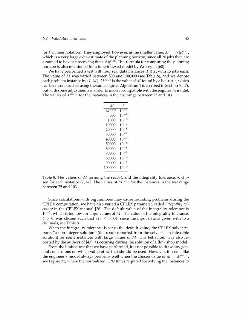
6.2 Validation and tests 45
(or P in their notation). They employed, however, as the smaller value,M = |J |pmaxj ,
which is a very large over-estimate of the planning horizon, since all 20 jobs then areassumed to have a processing time of pmax
j . This formula for computing the planninghorizon is also mentioned for a time-indexed model by Wolsey in [60].
We have performed a test with four real data instances, I ∈ I, with 15 jobs each.The value of M was varied between 500 and 100,000 (see Table 8), and we denoteeach problem instance by (I,M).Mheur is the value ofM found by a heuristic, whichhas been constructed using the same logic as Algorithm 1 (described in Section 5.4.7),but with some adjustments in order to make it compatible with the engineer’s model.The values of Mheur for the instances in the test range between 75 and 103.
M δMheur 10−5
500 10−6
1000 10−6
10000 10−7
20000 10−8
30000 10−8
40000 10−8
50000 10−8
60000 10−8
70000 10−8
80000 10−8
90000 10−8
100000 10−9
Table 8: The values of M forming the set M, and the integrality tolerance, δ, cho-sen for each instance (I,M). The values of Mheur for the instances in the test rangebetween 75 and 103.
Since calculations with big numbers may cause rounding problems during theCPLEX computation, we have also varied a CPLEX parameter, called integrality tol-erance in the CPLEX manual [26]. The default value of the integrality tolerance is10−5, which is too low for large values of M . The value of the integrality tolerance,δ > 0, was chosen such that Mδ ≤ 0.001, since the input data is given with twodecimals; see Table 8.
When the integrality tolerance is set to the default value, the CPLEX solver re-ports ”a non-integer solution” (the result reported from the solver is an infeasiblesolution) for some instances with large values of M . This behaviour was also re-ported by the authors of [43]; as occuring during the solution of a flow shop model.
From the limited test that we have performed, it is not possible to draw any gen-eral conclusions on which value of M that should be used. However, it seems likethe engineer’s model always performs well when the chosen value of M = Mheur;see Figure 22, where the normalized CPU times required for solving the instances to
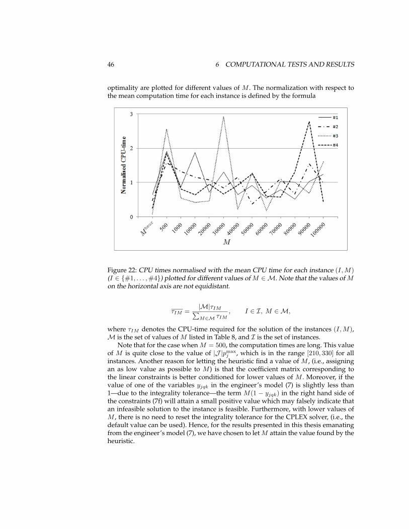
46 6 COMPUTATIONAL TESTS AND RESULTS
optimality are plotted for different values of M . The normalization with respect tothe mean computation time for each instance is defined by the formula
Figure 22: CPU times normalised with the mean CPU time for each instance (I,M)(I ∈ {#1, . . . ,#4}) plotted for different values of M ∈M. Note that the values of Mon the horizontal axis are not equidistant.
τIM =|M|τIM∑M∈M τIM
, I ∈ I, M ∈M,
where τIM denotes the CPU-time required for the solution of the instances (I,M),M is the set of values of M listed in Table 8, and I is the set of instances.
Note that for the case when M = 500, the computation times are long. This valueof M is quite close to the value of |J |pmax
j , which is in the range [210, 330] for allinstances. Another reason for letting the heuristic find a value of M , (i.e., assigningan as low value as possible to M ) is that the coefficient matrix corresponding tothe linear constraints is better conditioned for lower values of M . Moreover, if thevalue of one of the variables yjqk in the engineer’s model (7) is slightly less than1—due to the integrality tolerance—the term M(1 − yjqk) in the right hand side ofthe constraints (7f) will attain a small positive value which may falsely indicate thatan infeasible solution to the instance is feasible. Furthermore, with lower values ofM , there is no need to reset the integrality tolerance for the CPLEX solver, (i.e., thedefault value can be used). Hence, for the results presented in this thesis emanatingfrom the engineer’s model (7), we have chosen to letM attain the value found by theheuristic.
47
7 Conclusions
The problem of scheduling the multitask cell is proven to be NP-hard in Section 4.Therefore, in the search for the most efficient way to solve the problem to optimality,the choices of variable representation and optimization model is of great importance.
In this thesis several mathematical optimization models for solving the problemof scheduling the multitask cell are developed and presented: three models withinthe Manne family (4), (7), and (9), one time-discrete model with so-called nail vari-ables (11), and one time–discrete model with so-called plateau variables [(15)]. Wehave shown that model (11) outperforms the others by far with respect to computa-tion times and the sizes of instances that they are able to solve using standard opti-mization software. To our knowledge, this is the first model presented for the flexiblejob shop problem which employs the type of variables that are here called nail vari-ables. As mentioned in Section 3.1.1, most of the models for the job shop problempresented in scientific literature within operations research are members within theManne family (see [33]), and hence many researchers have developed similar models(see, e.g. [40, 14, 44] and [63]), not being aware of the potential of using nail variables.
A heuristic employed to determine the planning horizon, T , for the time-indexedmodels has been developed and is presented in Section 5.4.7. The use of this heuristicshortens the computation times substantially for all time-indexed models, comparedto the use of larger values of T , which are not specific for each instance.
Another parameter closely related to computation time is the length ` of the dis-cretization interval. We have estimated both the error due to the choice of the valueof ` and the impact of ` on the computation time, using data emanating from realproduction instances. For the current production in the multitask cell, we conclude,in Section 6.2.2, that ` = 1h is a suitable choice. The model (11) with ` = 1h requiredon average 40 CPU-seconds to find an optimal solution for scenarios with 45 jobs,which we estimate to be the largest size of a realistic instance for scheduling a com-ing shift. The relative error of the objective value will then be acceptable, with anaverage below 0.04%.
Another contribution of this thesis is the investigation of the effect on computa-tion time of the choice of the value of the model parameter M (within a model ofthe Manne family), which has to be large enough such that one can fit an optimalschedule within the time interval [0,M ] for a specific instance. Our test results, pre-sented in Section 6.2.4, show that ifM is chosen by a heuristic similar to Algorithm 1,then the computation times will be low in comparison with the use of larger or muchlarger values of M . This is contradictory to the results presented in [46] by Staffordet al. They chose, however, a much larger value than ours as the smallest value intheir test set, and, as it seems, did not consider the integrality tolerance employedby the software solver used. This tolerance needs to be reset for large values of M inorder to guarantee that a feasible solution is obtained.
48 8 FUTURE RESEARCH
8 Future research
Currently, in order to find a feasible schedule for the complete multitask cell—irres-pective of which of the models developed for the machining problem that is used—we need to employ the feasibility model (9). This model, which belongs to the Mannefamily, requires long computation times for instances with many jobs—too long to beacceptable in real applications. Since the time-indexed model (11) with nail variablesperforms very well, a subject for future research is to develop a time-indexed modeleither for the full problem, (that is, the problem of scheduling all resources in themultitask cell) or for the feasibility problem.
Another area for future research is to include the scheduling of fixtures, person-nel, and tools, in a mathematical optimization model for the problem of schedulingthe multitask cell; these resources are currently assumed to be unlimited, which isnot the case in the real application.
When performing all of the computations reported in this thesis, we assume thatthe data are reliable. We calculate, for example, the estimated arrivals of jobs to thecell, and then, sometimes, assign these value to the corresponding release dates. Ofcourse, we can not be certain that a part is going to be available at these releasedates, but fortunately the uncertainty decreases the closer the part is to the multitaskcell at time t0. This is good since we intend to produce a new schedule daily orat the beginning of every shift. An area for future research is to construct a robustoptimization model, which is less sensitive to data uncertainty. Other ideas are tofind ways of measuring the unability to follow a certain schedule caused by datauncertainty, or to produce alternative schedules on short notice for the case of, e.g.,machine break-downs.
As mentioned in Section 6.2, finding appropriate values of the weights of thecomponents of the objective functions used in the computational testing is an area offuture research. Instead of employing weighted objective functions, multiobjectiveoptimization theory can be applied to this problem, which is another area to explorewithin future research.
We have observed during the computational testing that the time-indexed modelwith nail variables (11) yields good lower bounds. The work on finding an evenstronger formulation of the problem of scheduling the multitask cell, and eventuallyso-called facets (the strongest formulation possible), is an ongoing master’s thesiswork at the department of Mathematical Sciences by a student from the Universityof Gothenburg. A study of the differences between the constraints (11e) and the alter-native constraints (14) is an interesting subject for this ongoing work and for futureresearch.
49
9 Summary of appended papers
Below follows a summary of the papers appended to this thesis. In addition to thesetwo papers, I am the main contributor of [52], [54], and [51].
9.1 Paper I — Optimization of schedules for a multitask produc-tion cell
In this paper, we compare production plans resulting from utilizing an earlier ver-sion of the time-indexed model with nail variables with schedules formed by thefirst–in–first–out (FIFO) and earliest–due–date (EDD) priority rules, which are sim-ilar to the methods used in the current manual planning of the multitask cell. Theproblem of scheduling the multitask cell is presented and the engineer’s model (7) ispresented. The current production planning prerequisites have been studied in orderto choose an appropriate objective function.
Six test scenarios have been used for the comparison. Three scenarios were cre-ated based on real production data from one day in March 2010. One scenario wasleft as it was, one was altered from the original scenario to include a larger propor-tion of short jobs, and the third was altered from the original scenario to include alarger proportion of long jobs. In these scenarios, all jobs are delayed at time t0 = 0.Three other scenarios were created analogously, however based on a constructed sce-nario of a high volume case. It is a realistic case of a future product mix, created bythe group planner working at the time in the multitask cell together with the masterplanner responsible for most of the products processed in the cell. In the three latterscenarios, approximately half of the jobs are already delayed at time t0 = 0. Each sce-nario consists of 20 jobs, which all are assumed to be checked-in into the multitaskcell, i.e., ready to be processed, at time t0 = 0.
In a discussion towards the end of the paper, there is a small example compris-ing three jobs showing the complexity of the combinatorial scheduling problem athand. We explain with this example how a priority rule will yield a schedule risk-ing both tardiness for the job with the least priority and lost capacity in one of thetwo machines in the example. The optimization model will, however, yield a betterschedule, which will make the multitask cell better prepared for the jobs yet to ar-rive. This is due to the fact that a priority rule only considers one job at a time, whilethe optimization model takes all jobs into account simultaneously.
Paper I is identical to [55] in the reference list.
9.2 Paper II — A note on the complexity of flow-shop schedulingwith deteriorating jobs
This paper is a note on an article named Complexity analysis of job-shop schedulingwith deteriorating jobs by G. Mosheiov [38], which claims to provide a complete anal-ysis of the complexity of flow-shop, open-shop and job-shop problems. A propor-tional deterioration rate is assumed, that is, the job processing times are increasing
50 9 SUMMARY OF APPENDED PAPERS
linear functions of the jobs’ starting times. The objective is the minimization of themakespan. Mosheiov introduces a polynomial-time algorithm for the two-machineflow-shop and open-shop problems and presents NP-hardness results for flow-shopsand open-shops with three or more machines and for job-shops with two or moremachines. The proof of NP-hardness for the flow-shop case is however not correct.Paper II provides a correct proof.
Paper II is identical to [53] in the reference list.
REFERENCES 51
References[1] J. ADAMS, E. BALAS, AND D. ZAWACK, The shifting bottleneck procedure for job shop schedul-
ing, Management Science, 34 (1988), pp. 391–401.
[2] M. AROSTEGUI, JR., S. KADIPASAOGLU, AND B. KHUMAWALA, An empirical comparisonof tabu search, simulated annealing, and genetic algorithms for facilities location problems, Inter-national Journal of Production Economics, 103 (2006), pp. 742–754.
[3] A. BAYKASOGLU AND L. ÖZBAKIR, Analyzing the effect of dispatching rules in the schedul-ing performance through grammar based flexible scheduling system, International Journal ofProduction Economics, 124 (2010), pp. 269–381.
[4] J. C. BECK, T. K. FENG, AND J.-P. WATSON, Combining constraint programming and localsearch for job-shop scheduling, INFORMS Journal on Computing, 23 (2011), pp. 1–14.
[5] J. H. BLACKSTONE, JR., D. T. PHILLIPS, AND G. L. HOGG, A state-of-the-art survey ofdispatching rules for manufacturing job shop operations, International Journal of ProductionResearch, 20 (1982), pp. 27–45.
[6] J. BŁAZEWICZ, K. H. ECKER, E. PESCH, G. SCHMIDT, AND J. WEGLARZ, Constraint pro-gramming and disjunctive scheduling, in Handbook on Scheduling, Springer Berlin Heidel-berg, 2007, pp. 477–538.
[7] E. H. BOWMAN, The schedule-sequencing problem, Operations Research, 7 (1959), pp. 621–624.
[8] P. BRUCKER, Scheduling Algorithms, Springer-Verlag, Berlin Heidelberg, 5th ed., 2007.
[9] P. BRUCKER, B. JURISCH, AND A. KRÄMER, Complexity of scheduling problems with multi-purpose machines, Annals of Operations Research, 70 (1997), pp. 57–73.
[10] K. BÜLBÜL AND P. KAMINSKY, A linear programming-based method for job shop schedul-ing. Available at http://www.optimization-online.org/DB_HTML/2010/12/2867.html, 2010.
[11] CSCMP SUPPLY CHAIN MANAGEMENT PROFESSIONALS, CSCMP supply chainmanagement definitions. Available at http://http://cscmp.org/aboutcscmp/definitions.asp.
[12] L. DE GIOVANNI AND F. PEZZELLA, An improved genetic algorithm for the distributed andflexible job-shop scheduling problem, European Journal of Operational Research, 200 (2010),pp. 395–408.
[13] K. FANG, N. A. UHAN, F. ZHAO, AND J. W. SUTHERLAND, Flow shop scheduling for sus-tainable manufacturing, in Proceedings of 10th Workshop on Models and Algorithms forPlanning and Scheduling Problems, Nymburk, Czech Republic, 2011.
[14] P. FATTAHI, M. SAIDI MEHRABAD, AND F. JOLAI, Mathematical modeling and heuristicapproaches to flexible job shop scheduling problems, Journal of Intelligent Manufacturing, 18(2007), pp. 331–342.
[15] R. FOURER, D. M. GAY, AND B. W. KERNIGHAN, AMPL: A Modeling Language for Math-ematical Programming, Brooks/Cole Publishing Company/Cengage Learning, 2nd ed.,2002.
[16] J. GAO, L. SUN, AND M. GEN, A hybrid genetic and variable neighborhood descent algo-rithm for flexible job shop scheduling problems, Computers & Operations Research, 35 (2008),pp. 2892–2907.
52 REFERENCES
[17] M. GAREY AND D. JOHNSON, Computers and intractability, W. H. Freeman & Co., NewYork, NY, USA, 1979.
[18] M. R. GAREY, D. S. JOHNSON, AND R. SETHI, The complexity of flowshop and jobshopscheduling, Mathematics of Operations Research, 1 (1976), pp. 117–129.
[19] M. GOMES, A. BARBOSA-PÓVOA, AND A.Q.NOVAIS, Optimal scheduling for flexible jobshop operation, International Journal of Production Research, 43 (2005), pp. 2323–2353.
[20] R. L. GRAHAM, E. L. LAWLER, J. K. LENSTRA, AND A. H. G. RINNOOY KAN, Opti-mization and approximation in deterministic sequencing and scheduling: A survey, Annals ofDiscrete Mathematics, 5 (1979), pp. 287–326.
[21] J. HEINONEN AND F. PETTERSSON, Hybrid ant colony optimization and visibility studies ap-plied to a job-shop scheduling problem, Applied Mathematics and Computation, 187 (2007),pp. 989–998.
[22] J. W. HERRMANN, Improving production scheduling: Integrating organizational, decision-making, and problem-solving perspectives, in Proceedings of the 2006 Industrial EngineeringResearch Conference May 20-24, Orlando, Florida, USA, 2006.
[23] A. B. HMIDA, M. HAOUARI, M.-J. HUGUET, AND P. LOPEZ, Discrepancy search for theflexible job shop scheduling problem, Computers & Operations Research, 37 (2010), pp. 2192–2201.
[24] O. HOLTHAUS AND C. RAJENDRAN, Efficient dispatching rules for scheduling in a job shop,International Journal of Production Economics, 48 (1997), pp. 87–105.
[25] W. J. HOPP AND M. L. SPEARMAN, Factory Physics, McGraw-Hill/Irwin, New York, NY,USA, 3d ed., 2008.
[26] IBM CORP., IBM ILOG CPLEX V12.1 User’s Manual for CPLEX, 2009.
[27] A. JAIN AND S. MEERAN, Deterministic job-shop scheduling: Past, present and future, Euro-pean Journal of Operational Research, 113 (1999), pp. 390–434.
[28] T. JANSSON, Resource utilization in a multitask cell, master’s thesis, Department of Mathe-matical Sciences, Chalmers University of Technology, Göteborg, Sweden, 2006.
[29] S. KEDAD-SIDHOUM, Y. R. SOLIS, AND F. SOURD, Lower bounds for the earliness-tardinessscheduling problem on single and parallel machines, European Journal of Operational Re-search, 189 (2008), pp. 1305–1316.
[30] A. KONONOV, Combinatorial complexity of scheduling jobs with simple linear deterioration,Discrete Analysis and Operations Research, 3 (1996), pp. 15–32.
[31] S. KREIPL AND J. DICKERSBACH, Scheduling coordination problems in supply chain planning,Annals of Operations Research, 161 (2008), pp. 103–122.
[32] L.LIBERTI AND J. OSTROWSKI, On the generation of symmetry breaking constraints for math-ematical programs, tech. report, Argonne National Laboratory, 9700 S. Cass Avenue Ar-gonne, IL 60439, France, July 2011.
[33] A. S. MANNE, On the job-shop scheduling problem, Operations Research, 8 (1960), pp. 219–223.
[34] F. MARGOT, Symmetry in integer linear programming, in 50 Years of Integer Programming1958-2008, M. Jünger, T. M. Liebling, D. Naddef, G. L. Nemhauser, W. R. Pulleyblank,G. Reinelt, G. Rinaldi, and L. A. Wolsey, eds., Springer Berlin, 2010, pp. 647–686.
REFERENCES 53
[35] D. MATTFELD AND C. BIERWIRTH, An efficient genetic algorithm for job shop scheduling withtardiness objectives, European Journal of Operational Research, 155 (2004), pp. 616–630.
[36] S. MEERAN AND M. MORSHED, A hybrid genetic tabu search algorithm for solving job shopscheduling problems: a case study, Journal of Intelligent Manufacturing, (2011). Available athttp://dx.doi.org/10.1007/s10845-011-0520-x.
[37] L. MÖNCH AND R. DRIESSEL, A distributed shifting bottleneck heuristic for complex job shops,Computers & Industrial Engineering, 49 (2005), pp. 363–380.
[38] G. MOSHEIOV, Complexity analysis of job-shop scheduling with deteriorating jobs, DiscreteApplied Mathematics, 117 (2002), pp. 195–209.
[39] G. L. NEMHAUSER AND L. A. WOLSEY, Integer and Combinatorial Optimization, John Wi-ley & Sons, Inc., New York, NY, USA, 1988.
[40] C. ÖZGÜVEN, L. ÖZBAKIR, AND Y. YAVUZ, Mathematical models for job-shop schedulingproblems with routing and process plan flexibility, Applied Mathematical Modelling, 34(2010), pp. 1539–1548.
[41] S. PETTERSSON, The interaction between optimization model and production at Volvo Aero,master’s thesis, Department of Technology Management and Economics, Chalmers Uni-versity of Technology, Göteborg, Sweden, 2010.
[42] M. E. POSNER, Job shop scheduling, in Wiley Encyclopedia of Operations Research andManagement Science, 2011.
[43] D. RONCONI AND E. BIRGIN, Mixed-integer programming models for flowshop schedulingproblems minimizing the total earliness and tardiness, in Just-in-Time Systems, Springer Se-ries on Optimization and Its Applications, vol. 60, 2011. Available at www.ime.usp.br/~egbirgin/publications/rob.pdf.
[44] J. ROSLÖF, I. HARJUNKOSKI, T. WESTERLUND, AND J. ISAKSSON, Solving a large-scale in-dustrial scheduling problem using MILP combined with a heuristic procedure, European Jour-nal of Operational Research, 138 (2002), pp. 29–42.
[45] J. SOUSA AND L. WOLSEY, A time indexed formulation of non-preemptive single machinescheduling problems, Mathematical Programming, 54 (1992), pp. 353–367.
[46] E. STAFFORD, JR., F. T. TSENG, AND J. N. D. GUPTA, Comparative evaluation of MILPflowshop models, The Journal of the Operational Research Society, 56 (2005), pp. 88–101.
[47] P. STOOP AND V. WIERS, The complexity of scheduling in practice, International Journal ofOperations & Production Management, 16 (1996), pp. 37–53.
[48] A. SYBERFELDT, A multi-objective evolutionary approach to simulation-based optimisation ofreal-world problems, PhD thesis, DeMontfort University, Leicester, UK, 2009.
[49] A. SYBERFELDT, A. NG, R. I. JOHN, AND P. MOORE, Multi-objective evolutionarysimulation-optimisation of a real-world manufacturing problem, Robotics and Computer-Integrated Manufacturing, 25 (2009), pp. 926–931.
[50] H. A. TAHA, Operations research: An introduction, Pearson Prentice Hall, Upper SaddleRiver, NJ, USA, 8th ed., 2007.
[51] K. THÖRNBLAD, T. ALMGREN, A.-B. STRÖMBERG, AND M. PATRIKSSON, Optimeringav scheman för en verklig produktionscell: tidsdiskretisering reducerar lösningstiden utan attlösningarnas kvalitet försämras, in PLANs forsknings- och tillämpningskonferens, Norr-köping, Sweden, 2011.

54 REFERENCES
[52] K. THÖRNBLAD AND L. KJELLSDOTTER IVERT, A comparison of schedules resulting frompriority rules and mathematical optimization for a real production cell, in PLANs forsknings-och tillämpningskonferens, Skövde, Sweden, 2010.
[53] K. THÖRNBLAD AND M. PATRIKSSON, A note on the complexity of flow-shop scheduling withdeteriorating jobs, Discrete Applied Mathematics, 159 (2011), pp. 251–253.
[54] K. THÖRNBLAD, M. PATRIKSSON, A.-B. STRÖMBERG, AND T. ALMGREN, Mathematicalmodelling of a real flexible job shop in aero engine component manufacturing, in Proceedingsof 10th Workshop on Models and Algorithms for Planning and Scheduling Problems,Nymburk, Czech Republic, 2011.
[55] K. THÖRNBLAD, A.-B. STRÖMBERG, T. ALMGREN, AND M. PATRIKSSON, Optimization ofschedules for a multitask production cell, in 22nd Nofoma conference proceedings, Kolding,Denmark, 2010.
[56] J. VAN DEN AKKER, C. HURKENS, AND M. SAVELSBERG, Time-indexed formulations for ma-chine scheduling problems: Column generation, INFORMS Journal on Computing, 12 (2000),pp. 111–124.
[57] T. VOLLMANN, W. L. BERRY, AND D. WHYBANK, Manufacturing Planning and ControlSystems, Irwin, Homewood IL, USA, 3d ed.
[58] H. M. WAGNER, An integer linear-programming model for machine scheduling, Naval Re-search Logistics Quarterly, 6 (1959), pp. 131–140.
[59] S. WANG AND J. YU, An effective heuristic for flexible job-shop scheduling problem with main-tenance activities, Computers & Industrial Engineering, 59 (2010), pp. 436–447.
[60] L. A. WOLSEY, MIP modelling of changeovers in production planning and scheduling problems,European Journal of Operational Research, 99 (1997), pp. 154–165.
[61] L. A. WOLSEY, Integer Programming, John Wiley & Sons, Inc., New York, NY, USA, 1998.
[62] R. ZHANG AND W. CHENG, A hybrid approach to large-scale job shop scheduling, AppliedIntelligence, 32 (2010), pp. 47–59.
[63] Z. ZHU AND R. HEADY, Minimizing the sum of earliness/tardiness in multi-machine schedul-ing: a mixed integer programming approach, Computers & Industrial Engineering, 38 (2000),pp. 297–305.