ON THE OPTIMAL REACHABILITY PROBLEM IN … THE OPTIMAL REACHABILITY PROBLEM IN WEIGHTED TIMED AUTOMATA AND GAMES Patricia Bouyer LSV, CNRS & ENS Cachan, France [email protected]

ON THE OPTIMAL REACHABILITYPROBLEM IN WEIGHTED TIMED

AUTOMATA AND GAMES

Patricia Bouyer

LSV, CNRS & ENS Cachan, [email protected]

AbstractIn these notes, we survey works made on the models of weighted timed automata and games,and more specifically on the optimal reachability problem.

1 Introduction

In thirty years computerized systems have widely spread in our society, from ubiquitous elec-tronic appliances (communication devices, automotive equipment, etc), to internet transactions(e-banking, e-business, etc), to new technologies (like wireless communications), and to criticalsystems (medical devices, industrial plants, etc). Due to their rapid development, such systemshave become more and more complex, and unfortunately this development has come with manybugs, from arithmetic overflow (which caused the crash of the Ariane 5 rocket in 1996) to raceconditions (which caused the lethal dysfunction of the Therac-25 radiotherapy machine in thelate 80’s) or infinite loops (for instance the leap-year bug turning all Zune MP3 devices off on31 December 2008). Many of those bugs could have been avoided if implemented softwareshad been formally verified prior to their use. The need for formal methods for verifying andcertifying computer-driven systems is therefore blatant.

Toward the development of more reliable computerized systems, several verification approacheshave been developed, among which the so-called model-checking technique. Model-checkingis a model-based approach to verification, which goes back to the late seventies [45, 31, 46].Given a system S and a property P , the model-checking approach consists in constructing amathematical model MS for the system and a mathematical model ϕP for the property, forwhich we will be able to automatically check that MS satisfies ϕP . If the models MS and ϕPare accurate enough with respect to S and P respectively, we will deduce with confidence thatthe system S satisfies the property P . This approach requires the development of expressivemodelling formalisms (to increase faithfulness of models) and efficient algorithms.

These last twenty years a huge effort has been made to design expressive models for representingcomputerized systems. As part of this effort the model of timed automata has been proposed

2 Patricia Bouyer

in the early nineties [4, 5], as a powerful and suitable model to reason about (the correct-ness of) real-time computerized systems. Timed automata extend finite-state automata withseveral clocks, which can be used to enforce timing constraints between various events in thesystem. They provide a convenient formalism and enjoy reasonably-efficient algorithms (e.g.reachability can be decided using polynomial space), which explains the enormous interest thatthey provoked in the community of formal methods. Timed games [8] extend timed automatawith a way of modelling systems interacting with external, uncontrollable components: sometransitions of the automaton cannot be forced or prevented to happen. The reachability prob-lem then asks whether there is a strategy to reach a given state, whatever the uncontrollablecomponents do. This problem can also be decided, in exponential time.

Timed automata and games are not powerful enough for representing quantities like resources,prices, temperature, etc. The more general model of hybrid automata [3, 2, 37, 38] (see [47] fora survey) allows for accurate modelling of such quantities using hybrid variables. The evolutionof these variables follow differential equations, depending on the state of the system, and thisunfortunately makes the reachability problem undecidable [38], even in the restricted case ofstopwatches, which are clocks that can be stopped and restarted.

Weighted (or priced) timed automata [6, 9] and games [42, 1, 17] have been proposed in the early2000’s as an intermediary model for modelling resource consumption or allocation problemsin real-time systems (eg optimal scheduling [11]). As opposed to (linear) hybrid systems,an execution in a weighted timed model is simply one in the underlying timed model: the extraquantitative information is just an observer of the system, and it does not modify the possiblebehaviours of the system. Figure 4 displays an example of a weighted timed game: each locationcarries an integer, which is the rate by which the weight (we will also call it cost thereafter)increases when time elapses in that location. Some edges also carry a weight, which indicateshow much the cost increases when crossing this edge. The cost of an execution is then theaccumulated sum of the costs of all individual moves along the execution, and this cost valueis a quantitative measure of the quality of the execution. Dashed edges are uncontrollable, andcannot be forced or prevented to occur; they appear in timed games only. Notice that theconstraints on edges never depend on the value of the cost, but only on the values of the clocks.

In these notes, we investigate the optimal reachability problem in weighted timed automataand games: given a target location, we want to know what is the optimal (i.e. smallest) cost forreaching the target location, and what is a corresponding strategy? We will survey the mainresults that have been obtained on that problem. We will start with a motivating example(Section 2). In Section 3, we will focus on the automaton model, state the main decidabilityresult, and give a glimpse of the new abstraction that may be used in this context. In Section 4,we will overview most of the results which have been obtained on this problem; we will alsogive some details on some of the technics that have been used. We will then show how we canuse the models studied in this paper to model the initial motivating example (Section 5).

ON THE OPTIMAL REACHABILITY PROBLEM IN WEIGHTED TIMED AUTOMATA AND GAMES3

2 An example: The task graph scheduling problem

In this section, we give an example of problem, that we will be able to model and solve usingthe developments presented in this paper.

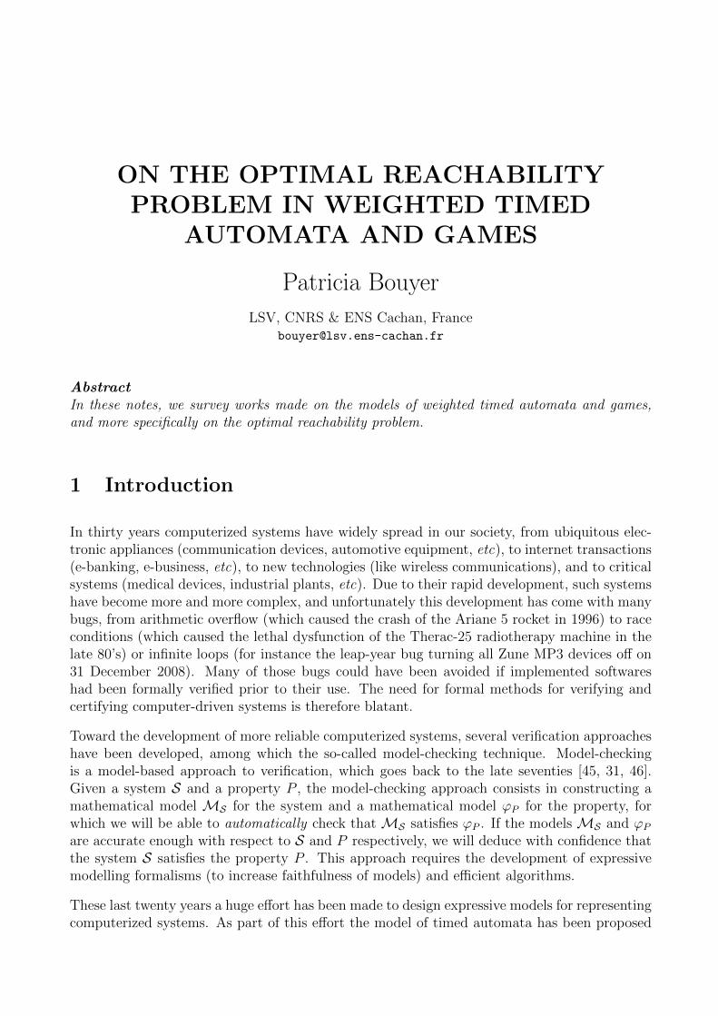
We want to compute the following arithmetical expression:

D×(C×(A+B))+(A+B)+(C×D)

using two processors, whose characteristics are given in Figure 1.

P1 (fast):

time+ 2 picoseconds× 3 picoseconds

energyidle 10 Watt

in use 90 Watts

P2 (slow):

time+ 5 picoseconds× 7 picoseconds

energyidle 20 Watts

in use 30 Watts

Figure 1: Characteristics of the two processors

+T1

×T2

×T3

+T4

×T5

+T6

BA DC

C

D

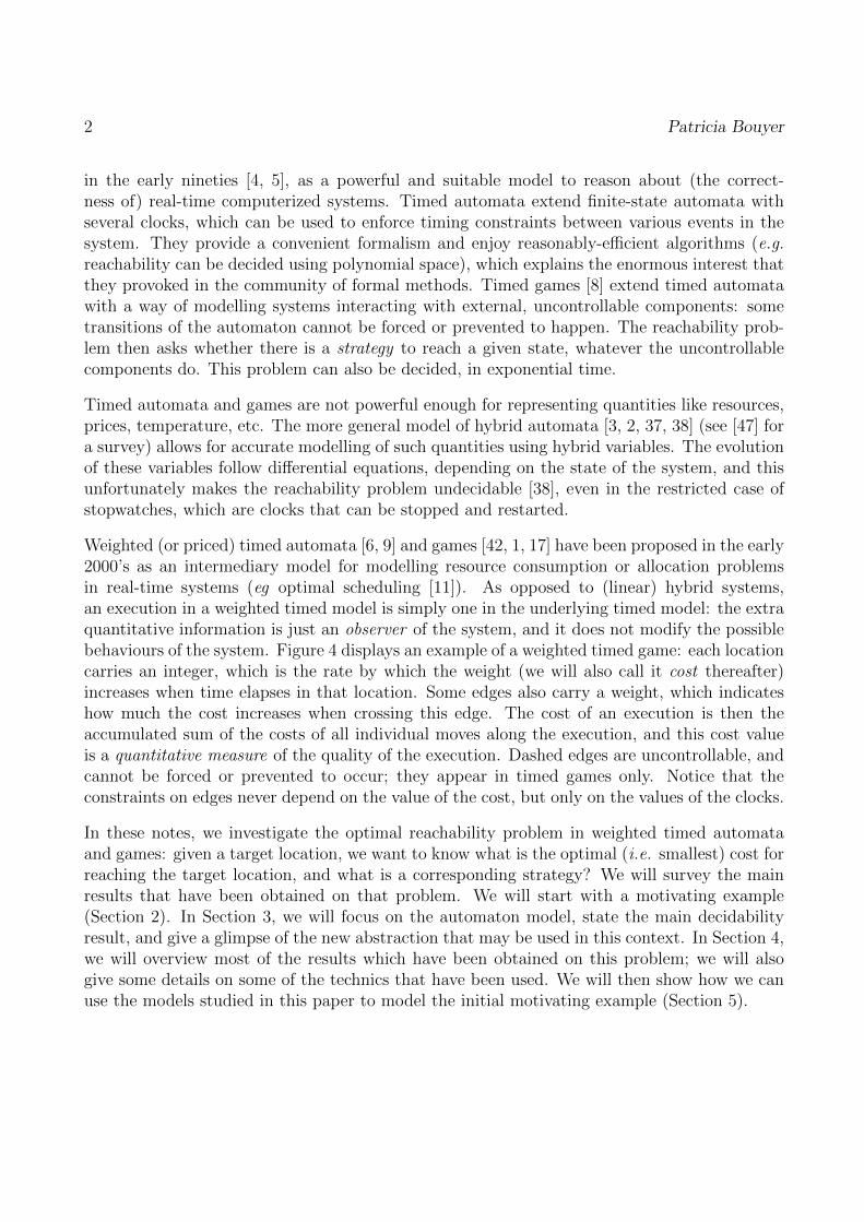
Figure 2: The task graph

The task graph giving the logical dependencies of the various atomic tasks that need to be donefor computing the arithmetical expression is depicted on Figure 2. It reads as follows: Task T3corresponds to the outermost multiplication in sub-expression C×(A+B). It requires first theaddition A+B to be computed, which is why the gate T3 has two inputs: C and the output ofT1 (implying that T1 needs to be computed prior to T3).

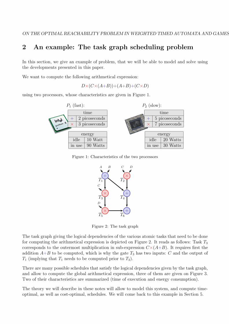
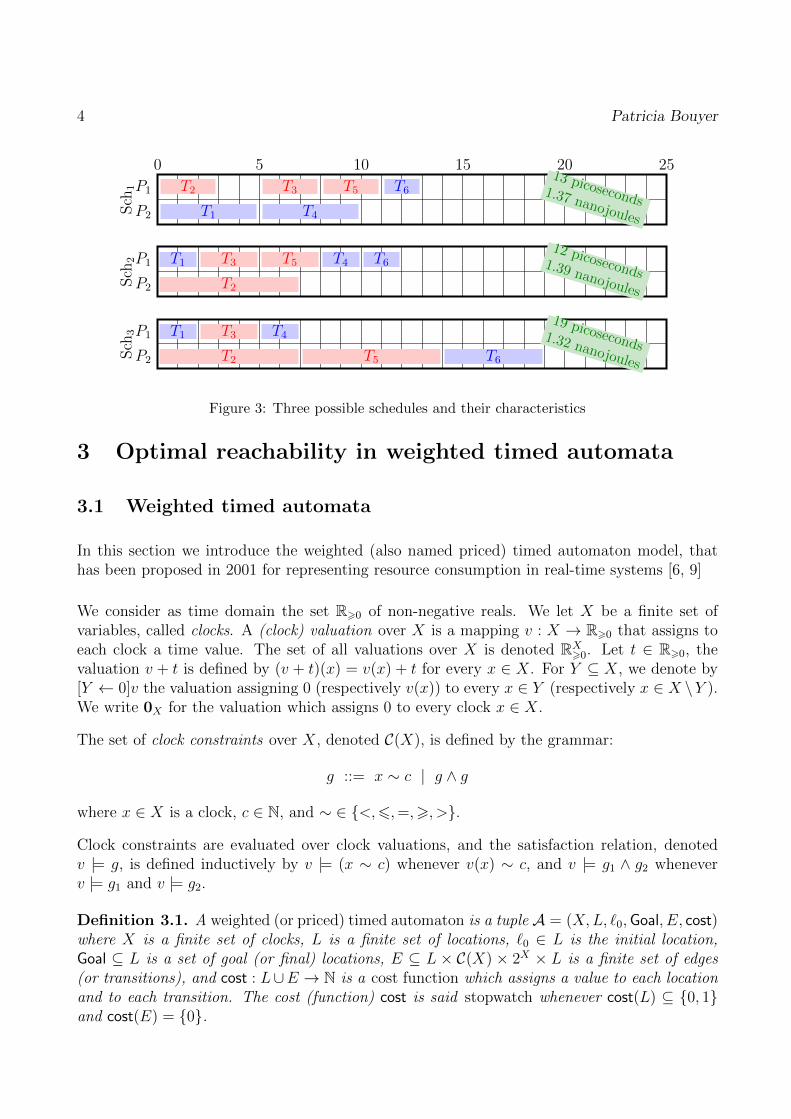
There are many possible schedules that satisfy the logical dependencies given by the task graph,and allow to compute the global arithmetical expression, three of them are given on Figure 3.Two of their characteristics are summarized (time of execution and energy consumption).

The theory we will describe in these notes will allow to model this system, and compute time-optimal, as well as cost-optimal, schedules. We will come back to this example in Section 5.

4 Patricia Bouyer

0 5 10 15 20 25

P2

P1

Sch

1 T2 T3 T5 T6

T1 T4

13 picoseconds1.37 nanojoules

P2

P1

Sch

2 T1

T2

T3 T4T5 T612 picoseconds

1.39 nanojoules

P2

P1

Sch

3 T1

T2

T3 T4

T5 T6

19 picoseconds1.32 nanojoules

Figure 3: Three possible schedules and their characteristics

3 Optimal reachability in weighted timed automata

3.1 Weighted timed automata

In this section we introduce the weighted (also named priced) timed automaton model, thathas been proposed in 2001 for representing resource consumption in real-time systems [6, 9]

We consider as time domain the set R>0 of non-negative reals. We let X be a finite set ofvariables, called clocks. A (clock) valuation over X is a mapping v : X → R>0 that assigns toeach clock a time value. The set of all valuations over X is denoted RX

>0. Let t ∈ R>0, thevaluation v + t is defined by (v + t)(x) = v(x) + t for every x ∈ X. For Y ⊆ X, we denote by[Y ← 0]v the valuation assigning 0 (respectively v(x)) to every x ∈ Y (respectively x ∈ X \Y ).We write 0X for the valuation which assigns 0 to every clock x ∈ X.

The set of clock constraints over X, denoted C(X), is defined by the grammar:

g ::= x ∼ c | g ∧ g

where x ∈ X is a clock, c ∈ N, and ∼ ∈ {<,6,=,>, >}.

Clock constraints are evaluated over clock valuations, and the satisfaction relation, denotedv |= g, is defined inductively by v |= (x ∼ c) whenever v(x) ∼ c, and v |= g1 ∧ g2 wheneverv |= g1 and v |= g2.

Definition 3.1. A weighted (or priced) timed automaton is a tuple A = (X,L, `0,Goal, E, cost)where X is a finite set of clocks, L is a finite set of locations, `0 ∈ L is the initial location,Goal ⊆ L is a set of goal (or final) locations, E ⊆ L × C(X) × 2X × L is a finite set of edges(or transitions), and cost : L∪E → N is a cost function which assigns a value to each locationand to each transition. The cost (function) cost is said stopwatch whenever cost(L) ⊆ {0, 1}and cost(E) = {0}.


In the above definition, if we forget about the cost function, we obtain the well-known model oftimed automata [4, 5]. The semantics of a weighted timed automaton is that of the underlyingtimed automaton, and the role of the cost function will be to give a quantitative informationto the moves and the executions in the system.

We therefore start by recalling the semantics of a timed automaton A = (X,L, `0,Goal, E).It is given as a timed transition system TA = (S, s0,→) where S = L × RX

>0 is the set ofconfigurations (or states) of A, s0 = (`0,0X) is the initial configuration, and → contains twotypes of moves:

• delay moves: (`, v)t−→ (`, v + t) if t ∈ R>0;

• discrete moves: (`, v)e−→ (`′, v′) if there exists an edge e = (`, g, Y, `′) in E such that v |= g,

v′ = [Y ← 0]v.

A run % in A is a finite or infinite sequence of moves in the transition system TA, with astrict alternation of delay moves (though possibly 0-delay moves) and discrete moves. In the

following, we may write a run % = st1−→ s′1

e1−→ s1t2−→ s′2

e2−→ s2 . . . more compactly as % = st1,e1−−→

s1t2,e2−−→ s2 . . .. A transition of the form s

t,e−→ s′ will be called a mixed move. If % is a finiterun which ends in some s = (`, v) with ` ∈ Goal, we say that % is accepting. If s ∈ S is aconfiguration, we write Runs(A, s) (respectively Runsf(A, s), Runsaccf (A, s)) the set of infinite(respectively finite, finite accepting) runs that start in s.

In the following we will assume timed automata are non-blocking, that is, from every reachableconfiguration s, there exists some delay t and some edge e, there exists some configuration s′

such that st,e−→ s′ is a mixed move of A.

We can now give the semantics of a weighted timed automaton A = (X,L, `0,Goal, E, cost).The value cost(`) given to location ` represents a cost rate, and delaying t time units in alocation ` will then cost ‘t ·cost(`)’. The value cost(e) given to edge e represents the cost oftaking that edge. Formally, the cost of the two types of moves in a weighted timed automatonis defined as follows:1 cost

((`, v)

t−→ (`, v + t))

= t · cost(`)

cost(

(`, v)e−→ (`′, v′)

)= cost(e)

A run % of a weighted timed automaton is a run of the underlying timed automaton, i.e., afinite or infinite sequence of moves in the transition system (with a strict alternation of delayand discrete moves). The cost of %, denoted cost(%), is the sum of the costs of all the simplemoves along %.

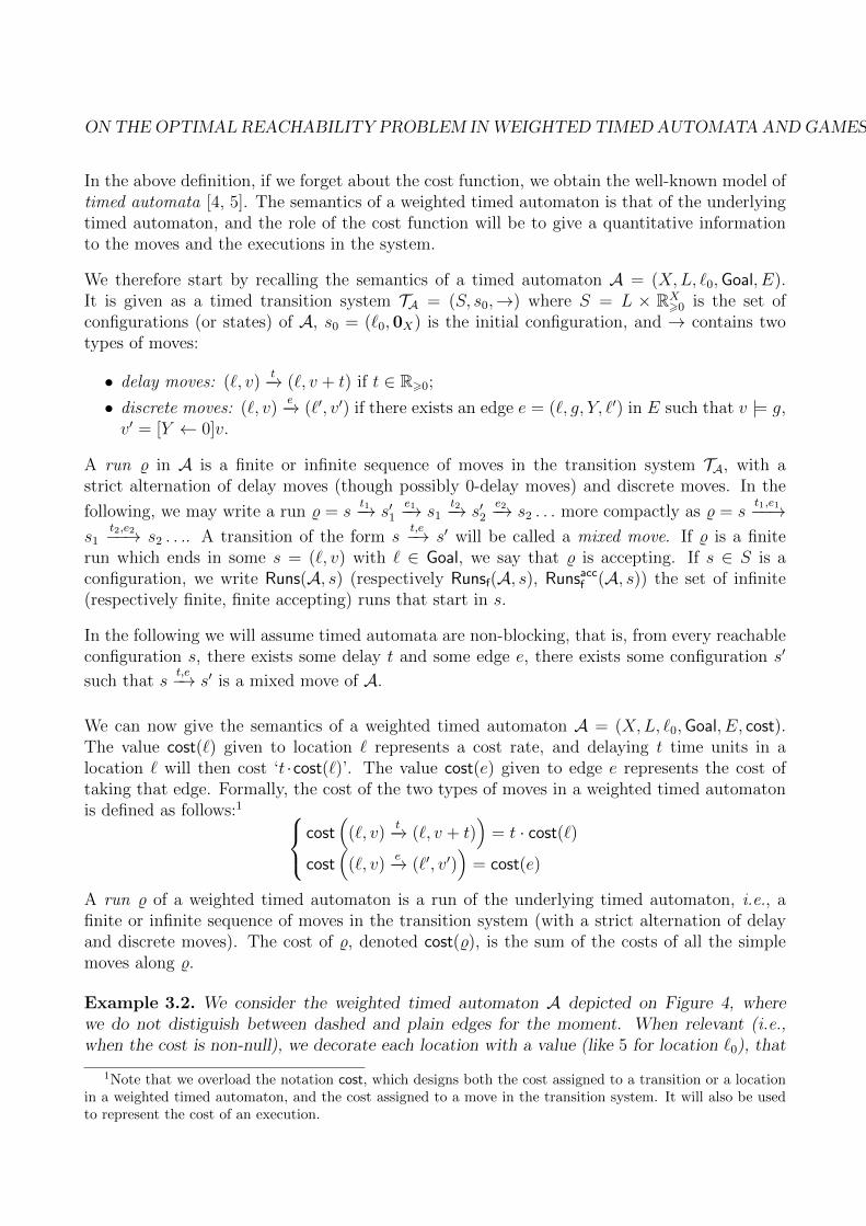
Example 3.2. We consider the weighted timed automaton A depicted on Figure 4, wherewe do not distiguish between dashed and plain edges for the moment. When relevant (i.e.,when the cost is non-null), we decorate each location with a value (like 5 for location `0), that

1Note that we overload the notation cost, which designs both the cost assigned to a transition or a locationin a weighted timed automaton, and the cost assigned to a move in the transition system. It will also be usedto represent the cost of an execution.

6 Patricia Bouyer

`0

5

`1

`2

10

`3

1

-x62, y:=0

e1

e2y=

0

e3y=0

x=2+1w2

x=2+7w3

Figure 4: A first small example

represents the cost rate in that location, and we decorate each edge with a value (like +7 foredge w3), that represents the discrete cost of taking that edge. A possible run in A is:

% = (`0, 0)0.1−→ (`0, 0.1)

e1−→ (`1, 0.1)e3−→ (`3, 0.1)

1.9−→ (`3, 2)w3−→ (,, 2)

The cost of % is cost(%) = 5 · 0.1 + 1 · 1.9 + 7 = 9.4 (the cost per time unit is 5 in `0, 1 in `3,and the cost of transition w3 is 7).

3.2 Optimization problems

Unlike hybrid systems, in weighted timed automata, cost variables do not constrain the be-haviours of the system, but are ‘observer variables’ : they give a quantitative information onthe quality (or performance) of an execution, but cannot impact on the possible executions.Several optimization criteria can then be thought of, like the optimal cost for reaching somegoal in the system, or the optimal mean-cost that can be achieved along infinite executionsof the system. These optimization problems are relevant for instance in scheduling problems,where the cost evolution can be viewed as resource consumption.

In this subsection we give an overview of the decidability and complexity results for the twooptimization problems we have mentioned. In the next subsection we will give a rough ideawhy these results hold.

3.2.1 The optimal cost problem

Intuitively, the optimal cost problem asks what is the optimal cost for reaching the goal locationsin a weighted timed automaton. We assume A = (X,L, `0,Goal, E, cost) is a weighted timedautomaton. The optimal cost for reaching goal locations in A is defined as:

opt costA = inf{cost(%) | % ∈ Runsaccf (A, s0)}

By extension when we will speak of the complexity, we will mean the complexity of the cor-responding decision problem, which asks, given a threshold c ∈ Q>0, whether opt costA 6 c.If ε > 0, a run % ∈ Runsf(A, s0) is an ε-optimal schedule in A if opt costA 6 cost(%) 6opt costA + ε.


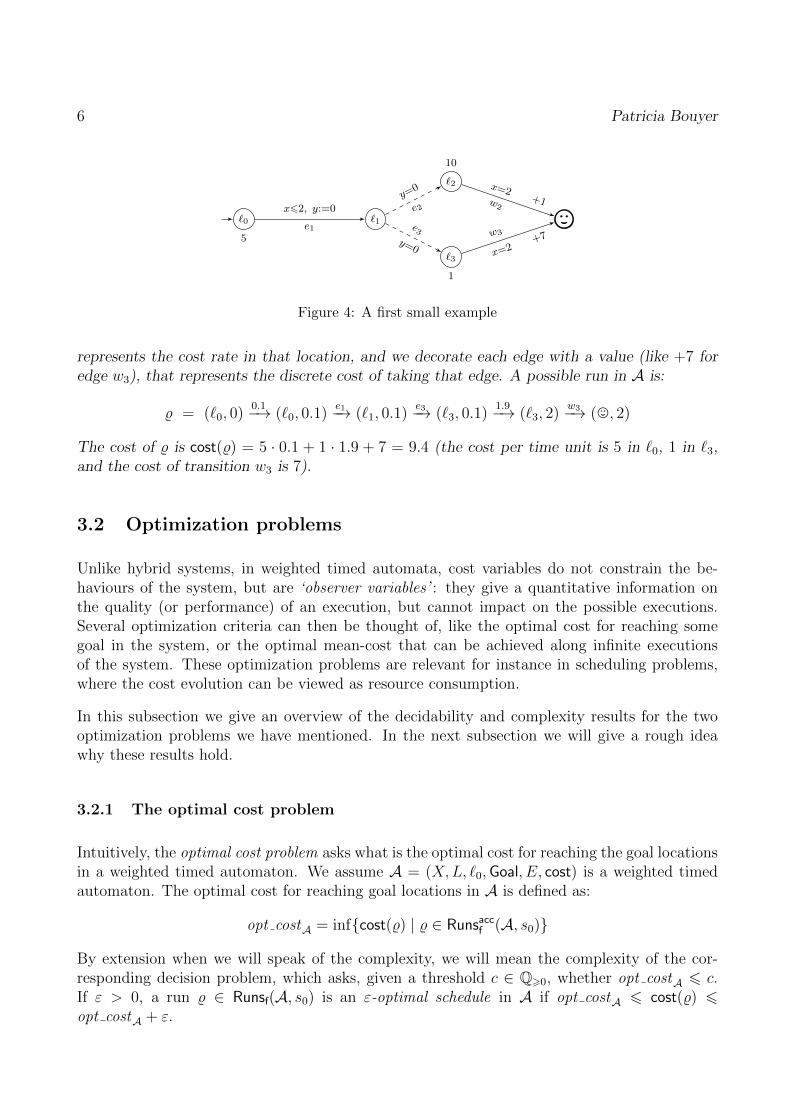
Example 3.3. We consider the weighted timed automaton of Example 3.2 (page 5). Thereare basically two choices that can be made: (i) when edge e1 is fired, and (ii) go through `2or through `3. Writing t for the value of clock x when e1 is fired, the accumulated cost alongplays of the game is either 5t+ 10(2− t) + 1 (through `2) or 5t+ (2− t) + 7 (through `3). Theoptimal cost is thus inft62 min(5t+ 10(2− t) + 1, 5t+ (2− t) + 7) = 9, and the optimal time forfiring transition e1 is when t = 0. Then, the best choice is to go through `3.

In this context, the first problem which has been solved already in the early nineties is theoptimal time problem, where the cost represents the time that has elapsed (the cost rates inlocations are equal to 1 — they increase at the same speed as the time — and discrete costs oftransitions are set to 0): the problem then amounts to computing the optimal time for reachingone of the distinguished goal locations in a timed automaton.

Theorem 3.4 ([33]). The optimal time in timed automata is computable in exponential time.

Applying the further results (theorem 3.6) on weighted timed automata, we can refine thisresult, and computing the optimal time in timed automata can actually be solved in polynomialspace. Moreover, we can prove that the corresponding decision problem is indeed PSPACE-complete (if there is an answer to the reachability problem, we can bound the duration of awitness run by an exponential, and then answering positively to the decision problem for thatupper bound duration is equivalent to answering the reachability question, which is known tobe PSPACE-hard).

Almost ten years after this first result, the general optimal cost optimal problem in weightedtimed automata has been formulated and solved independently in [6] and in [9].

Theorem 3.5 ([6, 9]). The optimal cost in weighted timed automata is computable (in expo-nential time).

The algorithm developed in [6] is based on an extension of the classical region automaton,and yields an EXPTIME upper bound, whereas the algorithm developed in [9] is based onwell-quasi-orders and gives no good information on the complexity of the problem.

Few years later, the precise complexity of that problem has been settled.

Theorem 3.6 ([13]). The optimal cost problem in weighted timed automata is PSPACE-complete.Furthermore, for every ε > 0, ε-optimal schedules can be computed.

Remark 3.7. Note that the above result also holds when the costs of locations on transitionsare taken in Z = N ∪ −N, the set of integers.

y

3.2.2 The optimal mean-cost problem

The optimal mean-cost problem asks what is the optimal cost per time unit (mean-cost) thatcan be achieved (or approximated) in a weighted timed automaton. To define the most general

8 Patricia Bouyer

mean-cost problem, we assume that A is a weighted timed automaton with two cost functions,say cost and reward (A = (X,L, `0,Goal, E, cost, reward). Then, the optimal mean-cost of Awith respect to cost and reward is formally defined as:

opt costωA = inf{mean cost(%) | % ∈ Runs(A, s0)}

where mean cost(%) is defined as lim infn→+∞

cost(%n)

reward(%n)(%n is the prefix of length n of %). We use

the ‘lim inf’ operator because the limit might not be properly defined. A particular case is whenthe reward corresponds to the time elapsed, in which case the value mean cost(%) is the meancost per time unit along run %. If ε > 0, a run % ∈ Runs(A, s0) is an ε-optimal schedule in A ifopt costωA 6 mean cost(%) 6 opt costωA + ε. The following result has been proven:

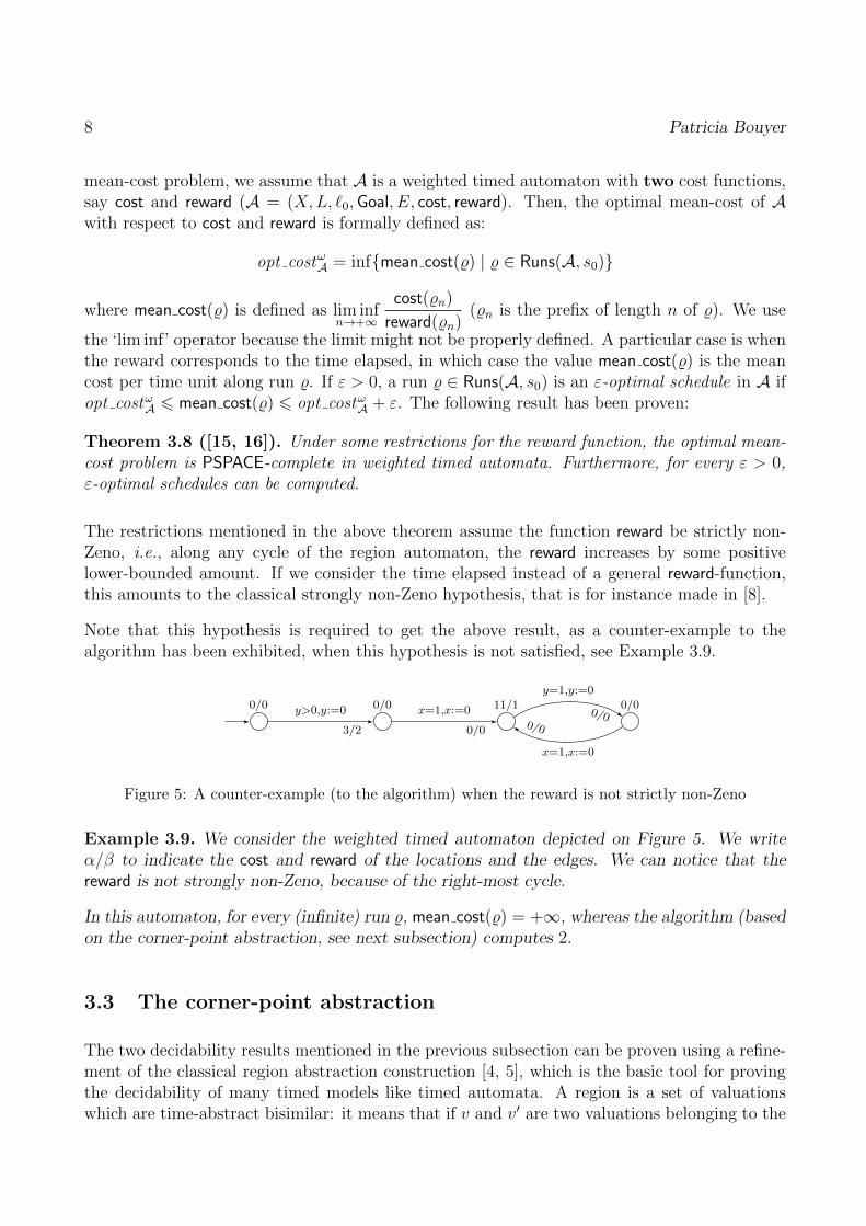
Theorem 3.8 ([15, 16]). Under some restrictions for the reward function, the optimal mean-cost problem is PSPACE-complete in weighted timed automata. Furthermore, for every ε > 0,ε-optimal schedules can be computed.

The restrictions mentioned in the above theorem assume the function reward be strictly non-Zeno, i.e., along any cycle of the region automaton, the reward increases by some positivelower-bounded amount. If we consider the time elapsed instead of a general reward-function,this amounts to the classical strongly non-Zeno hypothesis, that is for instance made in [8].

Note that this hypothesis is required to get the above result, as a counter-example to thealgorithm has been exhibited, when this hypothesis is not satisfied, see Example 3.9.

0/0 0/0 11/1 0/0y>0,y:=0

3/2

x=1,x:=0

0/0

y=1,y:=0

0/0

x=1,x:=0

0/0

Figure 5: A counter-example (to the algorithm) when the reward is not strictly non-Zeno

Example 3.9. We consider the weighted timed automaton depicted on Figure 5. We writeα/β to indicate the cost and reward of the locations and the edges. We can notice that thereward is not strongly non-Zeno, because of the right-most cycle.

In this automaton, for every (infinite) run %, mean cost(%) = +∞, whereas the algorithm (basedon the corner-point abstraction, see next subsection) computes 2.

3.3 The corner-point abstraction

The two decidability results mentioned in the previous subsection can be proven using a refine-ment of the classical region abstraction construction [4, 5], which is the basic tool for provingthe decidability of many timed models like timed automata. A region is a set of valuationswhich are time-abstract bisimilar: it means that if v and v′ are two valuations belonging to the


same region, for every location `, similar behaviours will be possible from (`, v) and (`, v′). Forthe readers not familiar with this construction, we refer to [12, Chap. 2.3] for a presentation ofthis classical construction, which uses notations and drawings similar to the current notes.

We first notice that regions are not suitable for computing optimal (mean-)costs because costsof region-equivalent trajectories may have pretty different costs. For example, the cost of run% given in Example 3.2 is 9.4 whereas the cost of the (region-equivalent) run delaying 0.9 timeunits in `0 and then 2.1 time units in `3 is 13.6. However we are not interested in computingthe costs of all possible runs, but rather to compute extremal (i.e., minimal and/or maximal)cost values. The idea is then to record the cost of moving through extremal points of theregions (those points which have integral coordinates). These points are called corner-points,and will annotate regions. We build a graph, called the corner-point abstraction, which refinesthe classical region automaton, and whose states are tuples (`, R, α) where ` is a location ofthe original automaton, R is a region, and α is a corner-point of R. There will be a (delay)transition between (`, R, α) and (`, R′, α′) either when R = R′ and α′ is a (strict) successor ofα, or when R′ is the next successor of R (in the region graph) and α′ = α is a corner of both Rand R′. There will be a (switch) transition between (`, R, α) and (`′, R′, α′) when (`′, R′) is theregion successor of (`, R) by the reset of the transition, and α′ is the image of α by the samereset. Intuitively, being in state (`, R, α) of this graph will mean that we are in location `, inregion R, close to the extremal point α; And moving from one state to another through a delaytransition means letting time elapse and be close to the designated corners. This constructionis illustrated and explained with some more intuition in Example 3.10.

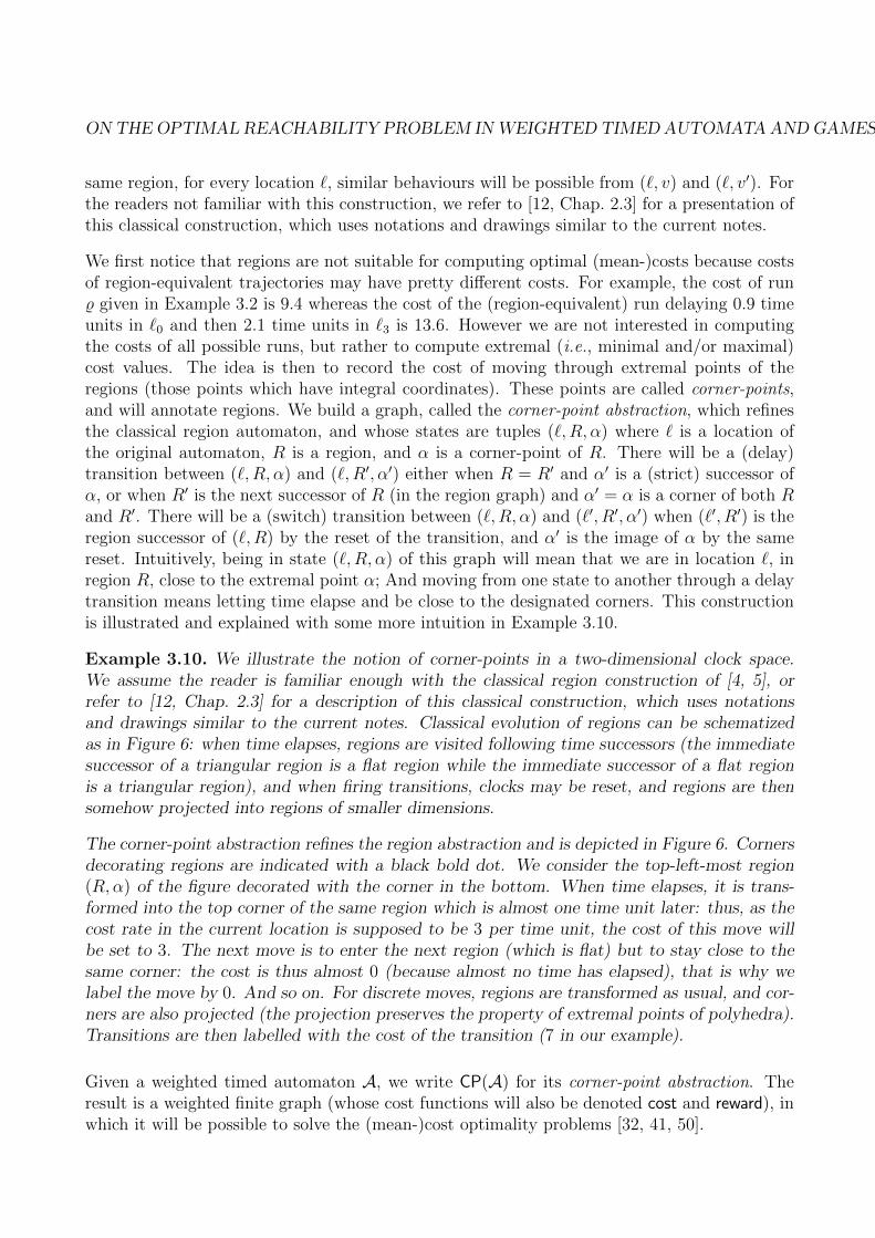
Example 3.10. We illustrate the notion of corner-points in a two-dimensional clock space.We assume the reader is familiar enough with the classical region construction of [4, 5], orrefer to [12, Chap. 2.3] for a description of this classical construction, which uses notationsand drawings similar to the current notes. Classical evolution of regions can be schematizedas in Figure 6: when time elapses, regions are visited following time successors (the immediatesuccessor of a triangular region is a flat region while the immediate successor of a flat regionis a triangular region), and when firing transitions, clocks may be reset, and regions are thensomehow projected into regions of smaller dimensions.

The corner-point abstraction refines the region abstraction and is depicted in Figure 6. Cornersdecorating regions are indicated with a black bold dot. We consider the top-left-most region(R,α) of the figure decorated with the corner in the bottom. When time elapses, it is trans-formed into the top corner of the same region which is almost one time unit later: thus, as thecost rate in the current location is supposed to be 3 per time unit, the cost of this move willbe set to 3. The next move is to enter the next region (which is flat) but to stay close to thesame corner: the cost is thus almost 0 (because almost no time has elapsed), that is why welabel the move by 0. And so on. For discrete moves, regions are transformed as usual, and cor-ners are also projected (the projection preserves the property of extremal points of polyhedra).Transitions are then labelled with the cost of the transition (7 in our example).

Given a weighted timed automaton A, we write CP(A) for its corner-point abstraction. Theresult is a weighted finite graph (whose cost functions will also be denoted cost and reward), inwhich it will be possible to solve the (mean-)cost optimality problems [32, 41, 50].

10 Patricia Bouyer

delay transition

discrete transition which resets yy

x

(a) The region abstraction

(R,α)

30 0

0

0 03

7

7

delay transition(cost rate 3)

discrete transition which resets y

(discrete cost 7)

(b) The corner-point abstraction

Figure 6: Region vs corner-point abstraction

An important property of this graph is that, given a finite run % : (`0, v0) → (`1, v1) → . . . →(`n, vn) in A, there exist two finite paths π : (`0, R0, α0) → (`1, R1, α1) → . . . → (`n, Rn, αn)and π′ : (`0, R0, α

′0)→ (`1, R1, α

′1)→ . . .→ (`n, Rn, α

′n) in CP(A) such that vi ∈ Ri for every i,

αi and α′i are corners of Ri, and cost(π) 6 cost(%) 6 cost(π′). Conversely, for every finite pathπ : (`0, R0, α0)→ (`1, R1, α1)→ . . .→ (`n, Rn, αn) in CP(A), for every ε > 0, we can constructa real run % : (`0, v0)→ (`1, v1)→ . . .→ (`n, vn) in A such that for every index i, vi ∈ Ri, and|cost(%)− cost(π)| < ε.

There is thus a strong relation between finite runs in A and finite paths in CP(A). Computingthe optimal cost for reaching a given goal in A reduces to computing the optimal cost forreaching a distinguished set of states in the discrete weighted graph CP(A).

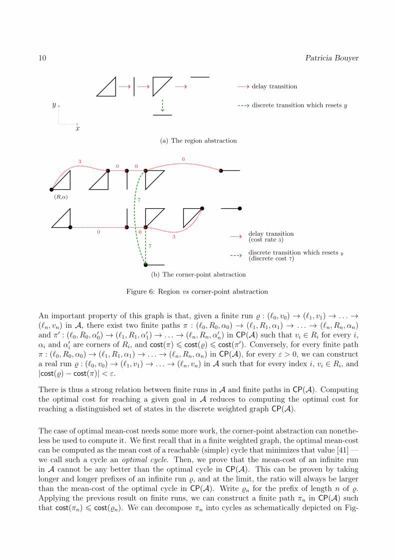
The case of optimal mean-cost needs some more work, the corner-point abstraction can nonethe-less be used to compute it. We first recall that in a finite weighted graph, the optimal mean-costcan be computed as the mean cost of a reachable (simple) cycle that minimizes that value [41] —we call such a cycle an optimal cycle. Then, we prove that the mean-cost of an infinite runin A cannot be any better than the optimal cycle in CP(A). This can be proven by takinglonger and longer prefixes of an infinite run %, and at the limit, the ratio will always be largerthan the mean-cost of the optimal cycle in CP(A). Write %n for the prefix of length n of %.Applying the previous result on finite runs, we can construct a finite path πn in CP(A) suchthat cost(πn) 6 cost(%n). We can decompose πn into cycles as schematically depicted on Fig-


ure 7. The linear part of πn is cycle-free, hence has a bounded length, and its cost will somehow

πn:

cycle-free

cycle appearing in πn

Figure 7: Decomposition of a long path in CP(A)

become negligible when n tends to +∞. The mean-cost of every cycle is no better than theoptimal cycle of CP(A). Hence, at the limit, the mean-cost of % will not be better than themean-cost of the optimal cycle in CP(A). Conversely, paths in the corner-point abstraction canbe approximated by real runs in the original automaton with costs and rewards that are veryclose to the one in the corner-point abstraction. The construction is presented in details in [16].

The size of the corner-point abstraction is exponential in the size of the original automaton (aregion R has at most |X| corner-points, where X is the set of clocks of the automaton), i.e.,as is the size of the region automaton. Using non-determinism, we can guess optimal paths(respectively cycles) in CP(A), without first computing the full graph. This non-deterministicalgorithm uses polynomial space, hence the PSPACE upper bound for the two optimizationproblems. The PSPACE lower bound can be easily obtained by reduction to the reachabilityproblem in timed automata, for appropriate cost functions.

3.4 Partial conclusion and related work

In this section, we have presented the decidability results for two basic optimization problemson weighted timed automata. This is really encouraging because the theoretical complexity ofthese problems is the same as standard reachability in timed automata.

In the context of (non-weighted) timed automata, regions are not used in implementations,but a symbolic approach based on zones is preferred and implemented. Similarly, a symbolicapproach for the optimal reachability problem based on priced zones, an extension of standardzones, has been proposed [43]. The paper [10] reports algorithms and applications of the toolUppaal-Cora,2 which is based on this approach. Also, when several cost variables are defined,it is possible to compute Pareto-optimal points [44]. On the contrary, the optimal mean-costis not implemented yet, since no good data structures have been developed. This is however avery challenging (and non-trivial) line of research.

We should emphasize that the corner-point abstraction is a very interesting abstraction, whichhas further been used for solving other optimization problems, like the time-discounted cost

2http://www.cs.aau.dk/~behrmann/cora/publications.html

http://www.cs.aau.dk/~behrmann/cora/publications.html

12 Patricia Bouyer

optimal problem [34] (this extends the classical discounted payoff that we can find in the gametheory literature [50]).

Finally, let us notice that even though one can compute the optimal (mean-)cost in weightedtimed automata, only almost-optimal schedules can be synthesized. The corner-point abtrac-tions does not allow to compute an optimal schedule, nor to decide that one exists.

4 Optimal reachability in weighted timed games

We have seen the optimal cost and the optimal mean-cost were both computable in weightedtimed automata in polynomial space. This is really encouraging to consider more involvedproblems. In this section, we consider the very similar problems, but no more in the context ofclosed systems, as in the previous section, but in the context of open systems. An open systemsomehow models an interaction between the system itself and the environment it is embeddedin. As often this is modelled as games [49] and we will use some terminology from game theory.

4.1 Weighted timed games

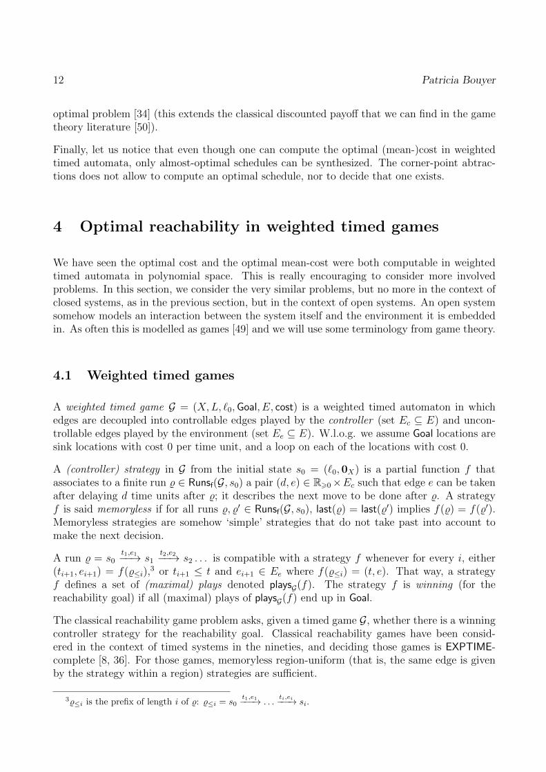
A weighted timed game G = (X,L, `0,Goal, E, cost) is a weighted timed automaton in whichedges are decoupled into controllable edges played by the controller (set Ec ⊆ E) and uncon-trollable edges played by the environment (set Ee ⊆ E). W.l.o.g. we assume Goal locations aresink locations with cost 0 per time unit, and a loop on each of the locations with cost 0.

A (controller) strategy in G from the initial state s0 = (`0,0X) is a partial function f thatassociates to a finite run % ∈ Runsf(G, s0) a pair (d, e) ∈ R>0×Ec such that edge e can be takenafter delaying d time units after %; it describes the next move to be done after %. A strategyf is said memoryless if for all runs %, %′ ∈ Runsf(G, s0), last(%) = last(%′) implies f(%) = f(%′).Memoryless strategies are somehow ‘simple’ strategies that do not take past into account tomake the next decision.

A run % = s0t1,e1−−→ s1

t2,e2−−→ s2 . . . is compatible with a strategy f whenever for every i, either(ti+1, ei+1) = f(%≤i),

3 or ti+1 ≤ t and ei+1 ∈ Ee where f(%≤i) = (t, e). That way, a strategyf defines a set of (maximal) plays denoted playsG(f). The strategy f is winning (for thereachability goal) if all (maximal) plays of playsG(f) end up in Goal.

The classical reachability game problem asks, given a timed game G, whether there is a winningcontroller strategy for the reachability goal. Classical reachability games have been consid-ered in the context of timed systems in the nineties, and deciding those games is EXPTIME-complete [8, 36]. For those games, memoryless region-uniform (that is, the same edge is givenby the strategy within a region) strategies are sufficient.

3%≤i is the prefix of length i of %: %≤i = s0t1,e1−−−→ . . .

ti,ei−−−→ si.


In the context of weighted timed games, an optimality criterion can be expressed. The cost ofa winning strategy f is defined as:

costG(f) = sup{cost(%) | % ∈ playsG(f)}

Note that if f is a winning strategy, then for every % ∈ playsG(f), cost(%) < +∞. However itmight be the case that costG(f) = +∞.

The aim of the controller is to optimize this value and we want to compute the optimal costthe controller can ensure, whatever the environment does, which can be formally written as:

opt costG = inf{costG(f) | f winning strategy}

We will consider the two following decision problems:

• the first, called the bounded cost problem, asks, given a threshold c ∈ Q>0, whether thereis some strategy f such that costG(f) 6 c;

• the second, called the optimal cost problem, asks, given a threshold c ∈ Q>0, whetheropt costG ≤ c.

We will also be interested in synthesizing almost-optimal strategies, that is for every ε > 0,computing a strategy fε which is ε-optimal : opt costG 6 costG(f) 6 opt costG + ε.

Example 4.1. We consider the weighted timed automaton of Example 3.2 (page 5). Dashed(respectively plain) arrows are now for uncontrollable (respectively controllable) transitions.Depending on the choice of the environment (going to location `2 or `3), the accumulated costalong plays of the game is either 5t+ 10(2− t) + 1 (through `2) or 5t+ (2− t) + 7 (through `3)where t is the delay elapsed in location `0. The optimal cost the controller can ensure is thusinft62 max(5t+10(2− t)+1, 5t+(2− t)+7) = 14+ 1

3, and the optimal time for firing transition

e1 is when t = 43. The controller has an optimal strategy, which consists in waiting in location

`0 until x = 43, and in entering location `1. Then, the environment chooses to go either to `2 or

to `3, and finally when the value of x reaches 2, the controller goes to the goal location ,.

Remark 4.2. Let us mention that in the above example, the optimal cost is non-integral,contrary to the case of closed systems. This means in particular that no region-based technology(and even corner-point abstraction) can be used to solve optimal timed games.

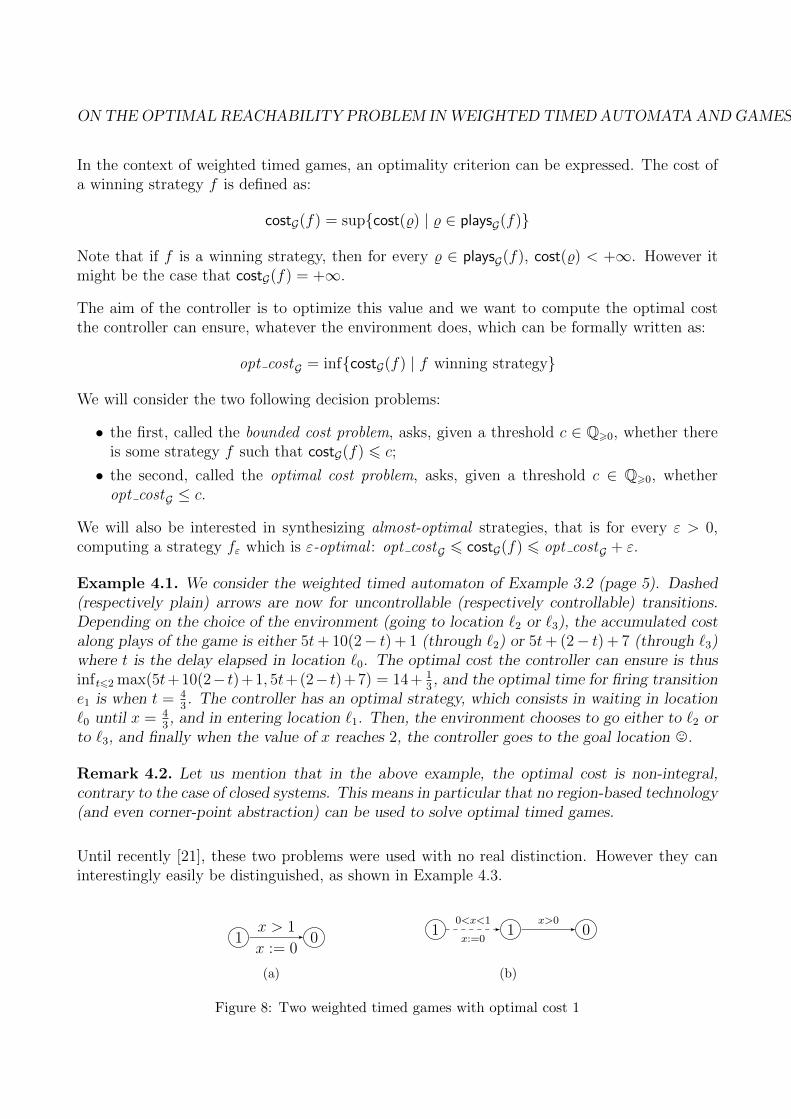
Until recently [21], these two problems were used with no real distinction. However they caninterestingly easily be distinguished, as shown in Example 4.3.

1 0x > 1

x := 0

(a)

1 1 00<x<1

x:=0

x>0

(b)

Figure 8: Two weighted timed games with optimal cost 1

14 Patricia Bouyer

Example 4.3. Consider the two weighted timed games depicted on Figure 8. In the game onthe left, for every ε > 0, the controller has a strategy to get cost 1 + ε. In the game on theright, the controller has a strategy to ensure cost strictly less than 1. Hence, in both cases, theoptimal cost is 1, but they generate quite different ‘behaviours’.

4.2 Decidability or undecidability?

In the late nineties, optimal-time timed games (i.e., weighted timed games where cost representstime elapsing) have been considered [7], and the complexity has been made precise ratherrecently [39] using strategy improvement techniques.

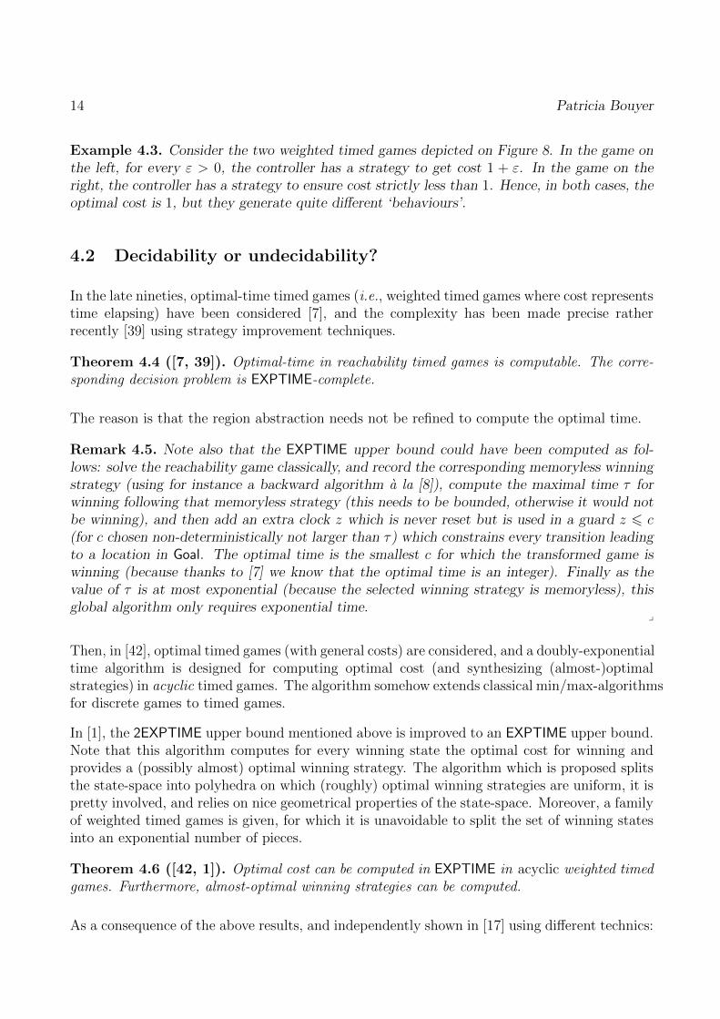
Theorem 4.4 ([7, 39]). Optimal-time in reachability timed games is computable. The corre-sponding decision problem is EXPTIME-complete.

The reason is that the region abstraction needs not be refined to compute the optimal time.

Remark 4.5. Note also that the EXPTIME upper bound could have been computed as fol-lows: solve the reachability game classically, and record the corresponding memoryless winningstrategy (using for instance a backward algorithm a la [8]), compute the maximal time τ forwinning following that memoryless strategy (this needs to be bounded, otherwise it would notbe winning), and then add an extra clock z which is never reset but is used in a guard z 6 c(for c chosen non-deterministically not larger than τ) which constrains every transition leadingto a location in Goal. The optimal time is the smallest c for which the transformed game iswinning (because thanks to [7] we know that the optimal time is an integer). Finally as thevalue of τ is at most exponential (because the selected winning strategy is memoryless), thisglobal algorithm only requires exponential time.

y

Then, in [42], optimal timed games (with general costs) are considered, and a doubly-exponentialtime algorithm is designed for computing optimal cost (and synthesizing (almost-)optimalstrategies) in acyclic timed games. The algorithm somehow extends classical min/max-algorithmsfor discrete games to timed games.

In [1], the 2EXPTIME upper bound mentioned above is improved to an EXPTIME upper bound.Note that this algorithm computes for every winning state the optimal cost for winning andprovides a (possibly almost) optimal winning strategy. The algorithm which is proposed splitsthe state-space into polyhedra on which (roughly) optimal winning strategies are uniform, it ispretty involved, and relies on nice geometrical properties of the state-space. Moreover, a familyof weighted timed games is given, for which it is unavoidable to split the set of winning statesinto an exponential number of pieces.

Theorem 4.6 ([42, 1]). Optimal cost can be computed in EXPTIME in acyclic weighted timedgames. Furthermore, almost-optimal winning strategies can be computed.

As a consequence of the above results, and independently shown in [17] using different technics:


Theorem 4.7 ([1, 17]). Under some restrictions for the cost function, the optimal cost andalmost-optimal winning strategies can be computed in weighted timed automata.

The restriction made in the above result is quite strong. It says that the cost needs to bestrongly non-Zeno: there is a constant κ > 0 such that every run that is read over a cycle ofthe region automaton has cost larger than κ. That means that the longer is a play, the largerwill be its cost; more precisely, if M is a bound on the cost of a given winning strategy (thatwe can choose memoryless and region-uniform), then we can unfold the game up to a depthwhich ensures that all runs will have cost larger than M , and solve this uncomplete unfoldedgame; this will preserve the optimal cost.

The first undecidability result has come as a surprise in [30]! It requires weighted timed gameswith five clocks. This result has been improved a bit later using a new encoding requiring onlythree clocks [14].

Theorem 4.8 ([30, 14]). The bounded cost problem for weighted timed games with three clocksor more is undecidable.

Note that, formally, this result does not speak of the optimal cost, but only of the existence ofa strategy whose cost is bounded by some constant (which is the bounded cost problem). Thisis some intriguing discrepancy with all known decidability results, which speak of the optimalcost problem. It has taken almost ten years for finally transferring this undecidability to theoptimal cost problem.

Theorem 4.9 ([21]). The optimal cost problem for weighted timed games with four clocks ormore is undecidable.

In Subsection 4.3, we will describe the undecidability proof of [14], which will help understandwhy it is so hard to analyze weighted timed games.

Is that the end of the story?

The previous undecidability result has settled the status of the optimal reachability problem inarbitrary weighted timed games, and has launched a quest for decidable subclasses of weightedtimed games. The first result in that direction is the following:

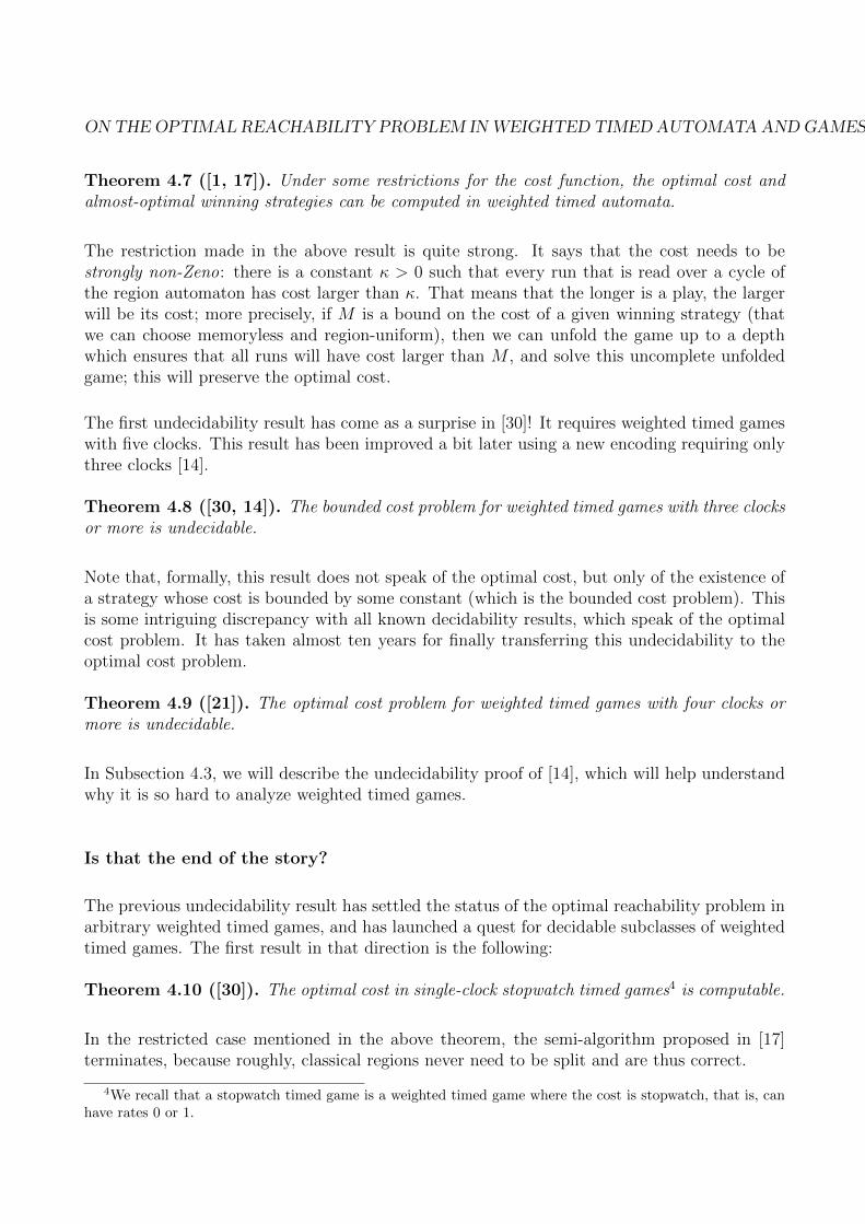
Theorem 4.10 ([30]). The optimal cost in single-clock stopwatch timed games4 is computable.

In the restricted case mentioned in the above theorem, the semi-algorithm proposed in [17]terminates, because roughly, classical regions never need to be split and are thus correct.

4We recall that a stopwatch timed game is a weighted timed game where the cost is stopwatch, that is, canhave rates 0 or 1.

16 Patricia Bouyer

Then, optimal cost in weighted timed games with one clock (but arbitrary cost) has beenproven computable [25] (though in a restricted turn-based framework where locations are eithercontrollable — i.e. all transitions leaving this location are controllable — or uncontrollable).The high complexity of the algorithm of [25] has later been improved in [48, 35], and a specialsubclass has been exhibited, in which optimal cost can be computed in PTIME. Technics usedin these papers make either use of structural properties of the game (like in [25]) or of valueiteration technics (like [35]).

Theorem 4.11 ([25, 48, 35, 28]). The optimal cost in turn-based single-clock weighted timedgames is computable in EXPTIME (PTIME if only two rates among {0,−d, d} for some d). Notethat the corresponding decision problem is PTIME-hard. Furthermore, for every ε > 0, we cancompute ε-optimal and memoryless strategies.

Another way to get around the undecidability results is to relax on the precision of the compu-tation. A recent result [21] builds on that idea, and proposes an approximation algorithm forthe optimal cost and for winning strategies. We believe that this is an interesting research direc-tion: indeed, in all decidability results that have been proven so far, even when the optimal costcan be computed, only almost-optimal strategies (or schedules, in the case of weighted timedautomata) can be synthesized. Hence, it seems that it is sufficient to compute an (arbitrary)approximate value of the optimal cost. More precisely, the result can be stated as follows:

Theorem 4.12 ([21]). Under some restrictions over the cost function, an arbitrary approx-imation of the optimal cost can be computed in weighted timed games. Furthermore, almost-optimal strategies can be computed as well.

We discuss now the restrictions mentioned in the theorem. They assume that the cost functionsatisfies the following condition: there exists some positive κ > 0 such that, if ρ is a run of theunderlying timed automaton which is read over a cycle of the region automaton, then:

(a) either cost(ρ) = 0;(b) or cost(ρ) ≥ κ.5

This restriction relaxes the strictly non-Zeno hypothesis made in Theorem 4.7, where all runsare required to satisfy condition (b). We should then insist on two things:

• First, as stated in Theorem 4.7, if (b) is always satisfied, the optimal cost can be computed;

• Then, the undecidability proofs for Theorems 4.8 and 4.9 (presented in Subsection 4.3)only build games that satisfy the restriction.

The complexity of the approximation is unfortunately not so good (2 exp(|G|) ·(

1/ε)|X|

, where

ε is the required precision). However the scheme might probably be improved to be turned intoa reasonably efficient algorithm. This is left as an open problem.

We will now give more details for the undecidability results, and for the approximation scheme.

5Similarly to the strongly non-Zeno hypothesis, we can take w.l.o.g. κ = 1.


4.3 A glimpse of the undecidability proof

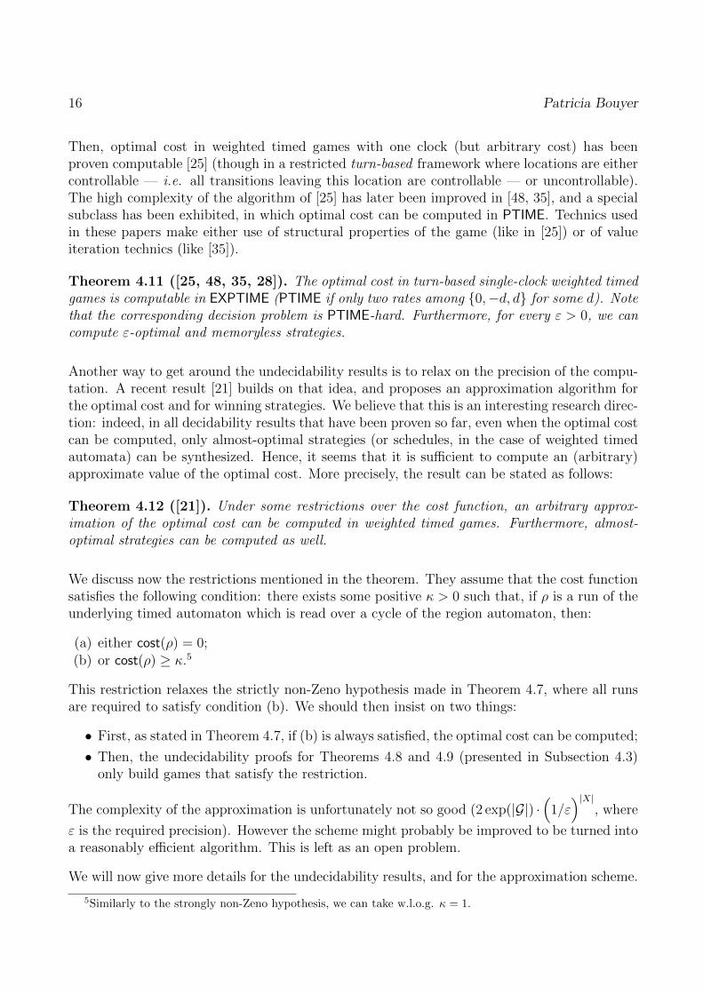
We will present the basic ideas of the undecidability proof proposed in [14] for Theorem 4.8,which we think is quite instructive. First we consider the two small modules that are depictedon Figure 9. The module Add+xz (x, y) (respectively Add+(1−x)

z (x, y)) uses z as an extra clock,lets the values of x and y at the end of the module be the same as at the entry of the module,increases the cost by x0 (respectively 1− x0) if x0 is the value of x when entering the module.

0 1

x=1,x:=0

y=1,y:=0 y=1,y:=0

z=1,z:=0z:=0

(a) Module Add+xz (x, y)

1 0

x=1,x:=0

y=1,y:=0 y=1,y:=0

z=1,z:=0z:=0

(b) Module Add+(1−x)z (x, y)

Figure 9: Two interesting modules

Concatenating these modules, one can implement various cost functions (non-negative linearcombinations of x0, y0, 1 − x0, 1 − y0 and 1). In particular, one can implement the two costfunctions cost1 and cost2 defined as follows:

cost1(x0, y0) = 2x0 + (1− y0) + 2 cost2(x0, y0) = 2(1− x0) + y0 + 1

Now, it is easy to check that 2x0 > y0 implies cost1(x0, y0) > 3, whereas 2x0 < y0 impliescost2(x0, y0) > 3. Moreover, if 2x0 = y0, then cost1(x0, y0) = cost2(x0, y0) = 3. Hence if weare in a state with x = x0 and y = y0, and if the choice of the cost function is given to theenvironment, it can enforce a cost (strictly) larger than 3 if and only if 2x0 6= y0. Otherwise,the cost will be 3, whatever is the choice of the environment. This will later serve as a moduleto check whether twice the value of x is equal to the value of y. We denote this test moduleTestz(2x = y), with the subscript z to indicate that an extra clock z is used in the module.

To simulate a two-counter machine, the idea is to store the value of a counter c into a clock,whose value will be, at distinguished points in time, 1

2c. Hence, to store the values of two

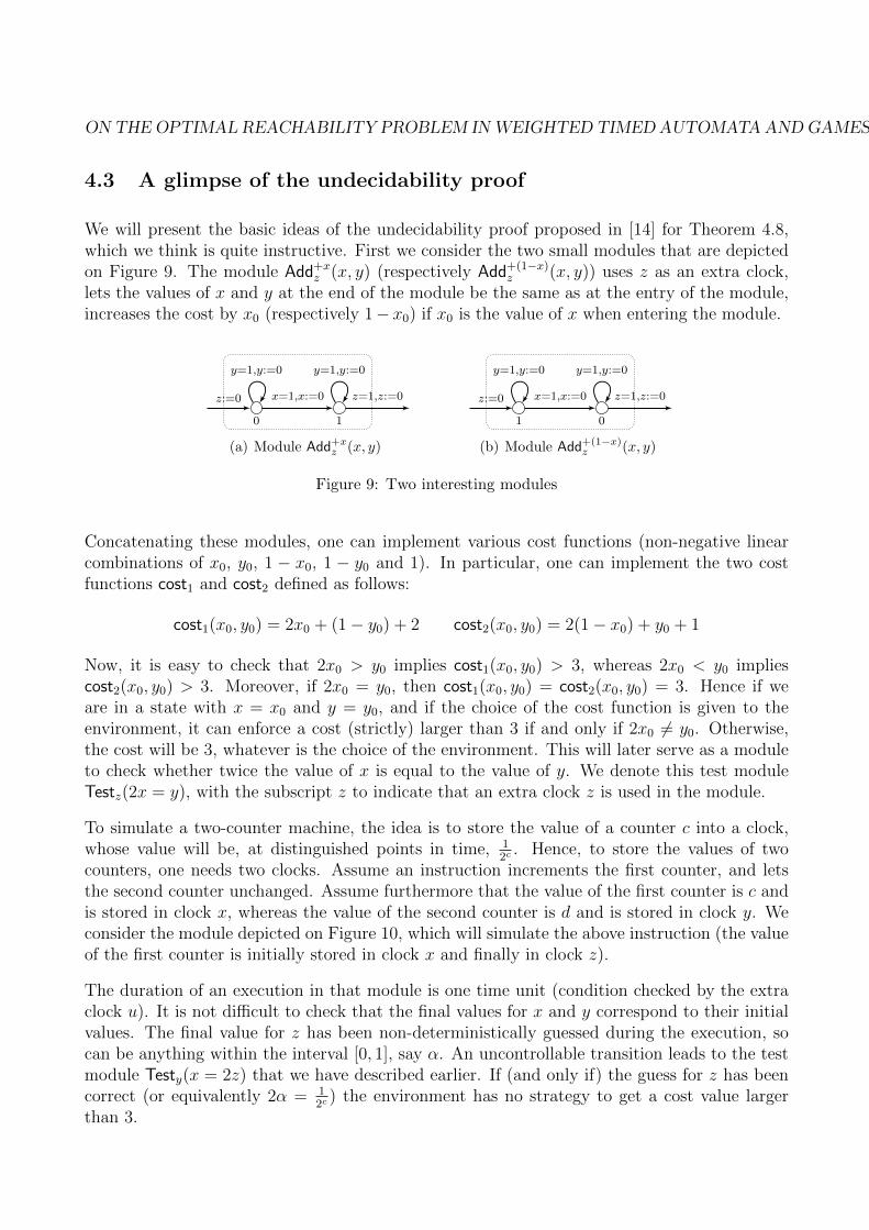
counters, one needs two clocks. Assume an instruction increments the first counter, and letsthe second counter unchanged. Assume furthermore that the value of the first counter is c andis stored in clock x, whereas the value of the second counter is d and is stored in clock y. Weconsider the module depicted on Figure 10, which will simulate the above instruction (the valueof the first counter is initially stored in clock x and finally in clock z).

The duration of an execution in that module is one time unit (condition checked by the extraclock u). It is not difficult to check that the final values for x and y correspond to their initialvalues. The final value for z has been non-deterministically guessed during the execution, socan be anything within the interval [0, 1], say α. An uncontrollable transition leads to the testmodule Testy(x = 2z) that we have described earlier. If (and only if) the guess for z has beencorrect (or equivalently 2α = 1

2c) the environment has no strategy to get a cost value larger

than 3.

18 Patricia Bouyer

x= 1

2c

y= 1

2d

z=?

u:=0 z:=0

x=1,x:=0∨ y=1,y:=0

x=1,x:=0∨ y=1,y:=0

x= 1

2c

y= 1

2d

z=α

u=1,u:=0

Testy(x=2z)

u=0

Figure 10: Simulation of the instruction which increments c and lets d unchanged

There is no cost labelling locations of the main game, we only add a discrete cost of +3 (orthree time units with cost-rate 1) when reaching the halting state. In that reduction:

the two-counter machine halts if, and only if,the controller has a winning strategy with cost no more than 3

in the weighted timed game.

It is worth noticing that the described reduction uses four clocks, and not three, as claimed.However, we can get rid of clock u using the following trick: the value of the second counter dis now stored by the value 1

3d(note that the choice of 1

2cand 1

3dis arbitrary, it could be 1

pcand

1qd

for p and q relatively prime integers). Indeed we can prove that the constraint u = 1 at theend of the module can be replaced by the constraints that the value of x is a negative power of2 and the value of y is a negative power of 3. Testing that the value of x is a negative powerof 2 can be done by iteratively multiplying the value of x by 2 (done using the Testy(z = 2x)module) and eventually reaching 1. Finally the constraint that the last location of the modulebe transient is done by adding a positive cost to that location, and requiring the controller tohave a strategy with cost no more than 3.

We can finally notice that the cost in this constructed game is stopwatch (there is no discretecost, and all cost rates are 0 or 1).

4.4 A glimpse of the approximation scheme

We quickly describe in this subsection the approximation scheme used in Theorem 4.12. Wefix a weighted timed game G = (X,L, `0,Goal, E, cost), and we split it along regions.6 Thekernel K of G is the part in which all runs have cost 0: it is made of locations with cost-rate 0,and edges with cost 0. The idea is that sub-runs in K do not impact on the global cost of theexecution, but it does impact on the clock values; on the other hand, sub-runs outside of thekernel have an important impact on the cost of the execution, hence they cannot be too long.

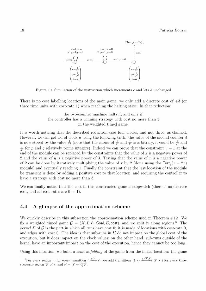
Using this intuition, we build a semi-unfolding of the game from the initial location: the game

6For every region r, for every transition `g,Y−−→ `′, we add transitions (`, r)

g∧−→r ,Y−−−−−→ (`′, r′) for every time-successor region −→r of r, and r′ = [Y ← 0]−→r .


is unfolded, and once the kernel is entered, a (folded) copy of the kernel is plugged; the gameis unfolded again from the output edges of the kernel. We stop unfolding when the depth ofthis semi-unfolding is N = (M + 2) · |R(G)|, where |R(G)| is the size of the region automatonof G and M is an upper bound on opt costG.

7 This enforces that all runs from the root to aleaf has a cost larger than what should be generated by an (almost-)optimal strategy. Hencethe optimal cost in the original game and in the semi-unfolding coincide. The construction isillustrated on Figure 11.

(`,r)

Only cost 0Kernel K

Only cost 0Kernel K

(`,r)

Hypothesis:cost > 0 implies cost ≥ 1

Figure 11: Semi-unfolding of game G

Exact computation

Approximation

Figure 12: Approximation scheme

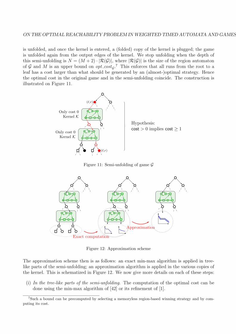
The approximation scheme then is as follows: an exact min-max algorithm is applied in tree-like parts of the semi-unfolding; an approximation algorithm is applied in the various copies ofthe kernel. This is schematized in Figure 12. We now give more details on each of these steps:

(i) In the tree-like parts of the semi-unfolding. The computation of the optimal cost can bedone using the min-max algorithm of [42] or its refinement of [1].

7Such a bound can be precomputed by selecting a memoryless region-based winning strategy and by com-puting its cost.

20 Patricia Bouyer

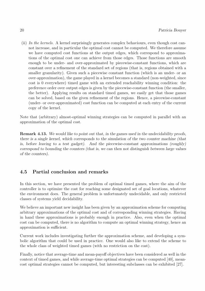
(ii) In the kernels. A kernel surprisingly generates complex behaviours, even though cost can-not increase, and in particular the optimal cost cannot be computed. We therefore assumewe have computed cost functions at the output edges, which correspond to approxima-tions of the optimal cost one can achieve from those edges. Those functions are smoothenough to be under- and over-approximated by piecewise-constant functions, which areconstant over a refinement of the standard set of regions (that is, regions obtained with asmaller granularity). Given such a piecewise constant function (which is an under- or anover-approximation), the game played in a kernel becomes a standard (non-weighted, sincecost is 0 everywhere) timed game with an extended reachability winning condition: thepreference order over output edges is given by the piecewise-constant function (the smaller,the better). Applying results on standard timed games, we easily get that those gamescan be solved, based on the given refinement of the regions. Hence, a piecewise-constant(under- or over-approximated) cost function can be computed at each entry of the currentcopy of the kernel.

Note that (arbitrary) almost-optimal winning strategies can be computed in parallel with anapproximation of the optimal cost.

Remark 4.13. We would like to point out that, in the games used in the undecidability proofs,there is a single kernel, which corresponds to the simulation of the two counter machine (thatis, before leaving to a test gadget). And the piecewise-constant approximations (roughly)correspond to bounding the counters (that is, we can then not distinguish between large valuesof the counters).

4.5 Partial conclusion and remarks

In this section, we have presented the problem of optimal timed games, where the aim of thecontroller is to optimize the cost for reaching some designated set of goal locations, whateverthe environment does. The general problem is unfortunately undecidable, and only restrictedclasses of systems yield decidability.

We believe an important new insight has been given by an approximation scheme for computingarbitrary approximations of the optimal cost and of corresponding winning strategies. Havingin hand these approximations is probably enough in practice. Also, even when the optimalcost can be computed, there is no algorithm to compute an optimal winning strategy, hence anapproximation is sufficient.

Current work includes investigating further the approximation scheme, and developing a sym-bolic algorithm that could be used in practice. One would also like to extend the scheme tothe whole class of weighted timed games (with no restriction on the cost).

Finally, notice that average-time and mean-payoff objectives have been considered as well in thecontext of timed games, and while average-time optimal strategies can be computed [40], mean-cost optimal strategies cannot be computed, but interesting subclasses can be exhibited [27].


5 Back to the task graph scheduling example

We come back to the example we have described in Section 2.

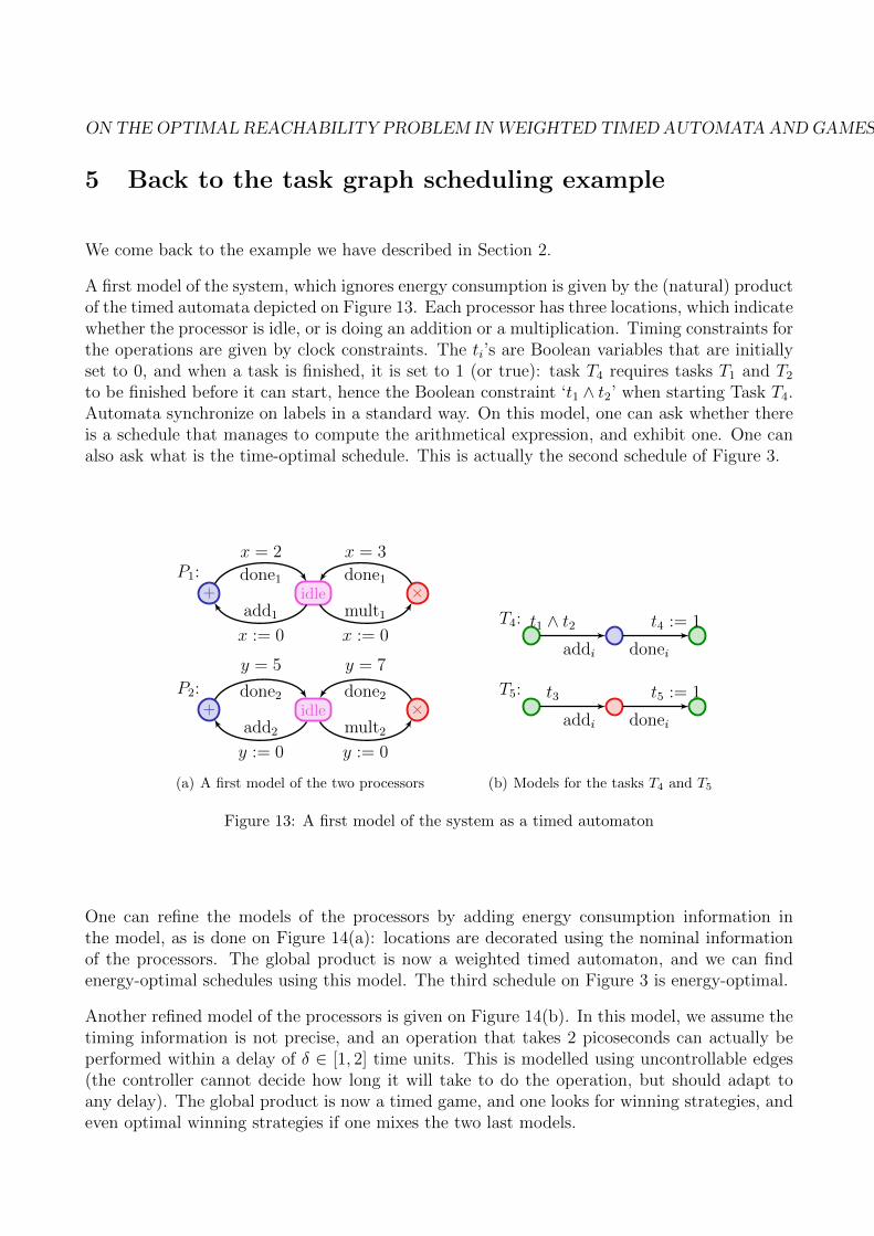
A first model of the system, which ignores energy consumption is given by the (natural) productof the timed automata depicted on Figure 13. Each processor has three locations, which indicatewhether the processor is idle, or is doing an addition or a multiplication. Timing constraints forthe operations are given by clock constraints. The ti’s are Boolean variables that are initiallyset to 0, and when a task is finished, it is set to 1 (or true): task T4 requires tasks T1 and T2to be finished before it can start, hence the Boolean constraint ‘t1 ∧ t2’ when starting Task T4.Automata synchronize on labels in a standard way. On this model, one can ask whether thereis a schedule that manages to compute the arithmetical expression, and exhibit one. One canalso ask what is the time-optimal schedule. This is actually the second schedule of Figure 3.

P1:idle+ ×

x := 0

add1

x := 0

mult1

x = 2

done1

x = 3

done1

P2:idle+ ×

y := 0

add2

y := 0

mult2

y = 5

done2

y = 7

done2

(a) A first model of the two processors

T4: t1 ∧ t2addi

t4 := 1

donei

T5: t3

addi

t5 := 1

donei

(b) Models for the tasks T4 and T5

Figure 13: A first model of the system as a timed automaton

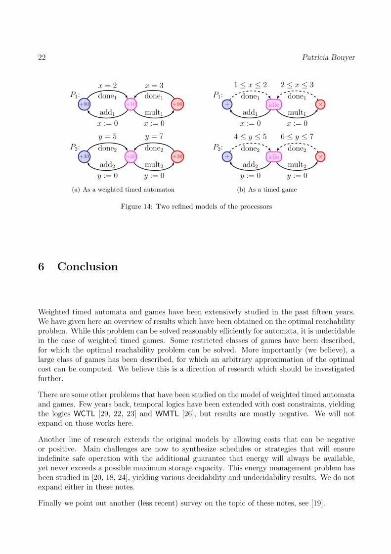
One can refine the models of the processors by adding energy consumption information inthe model, as is done on Figure 14(a): locations are decorated using the nominal informationof the processors. The global product is now a weighted timed automaton, and we can findenergy-optimal schedules using this model. The third schedule on Figure 3 is energy-optimal.

Another refined model of the processors is given on Figure 14(b). In this model, we assume thetiming information is not precise, and an operation that takes 2 picoseconds can actually beperformed within a delay of δ ∈ [1, 2] time units. This is modelled using uncontrollable edges(the controller cannot decide how long it will take to do the operation, but should adapt toany delay). The global product is now a timed game, and one looks for winning strategies, andeven optimal winning strategies if one mixes the two last models.

22 Patricia Bouyer

P1:+10+90 +90

x := 0

add1

x := 0

mult1

x = 2

done1

x = 3

done1

P2:+20+30 +30

y := 0

add2

y := 0

mult2

y = 5

done2

y = 7

done2

(a) As a weighted timed automaton

P1:idle+ ×

x := 0

add1

x := 0

mult1

1 ≤ x ≤ 2

done1

2 ≤ x ≤ 3

done1

P2:idle+ ×

y := 0

add2

y := 0

mult2

4 ≤ y ≤ 5

done2

6 ≤ y ≤ 7

done2

(b) As a timed game

Figure 14: Two refined models of the processors

6 Conclusion

Weighted timed automata and games have been extensively studied in the past fifteen years.We have given here an overview of results which have been obtained on the optimal reachabilityproblem. While this problem can be solved reasonably efficiently for automata, it is undecidablein the case of weighted timed games. Some restricted classes of games have been described,for which the optimal reachability problem can be solved. More importantly (we believe), alarge class of games has been described, for which an arbitrary approximation of the optimalcost can be computed. We believe this is a direction of research which should be investigatedfurther.

There are some other problems that have been studied on the model of weighted timed automataand games. Few years back, temporal logics have been extended with cost constraints, yieldingthe logics WCTL [29, 22, 23] and WMTL [26], but results are mostly negative. We will notexpand on those works here.

Another line of research extends the original models by allowing costs that can be negativeor positive. Main challenges are now to synthesize schedules or strategies that will ensureindefinite safe operation with the additional guarantee that energy will always be available,yet never exceeds a possible maximum storage capacity. This energy management problem hasbeen studied in [20, 18, 24], yielding various decidability and undecidability results. We do notexpand either in these notes.

Finally we point out another (less recent) survey on the topic of these notes, see [19].


Acknowledgements

This work is supported by ERC Project EQualIS (FP7-308087). I would like to thank all myco-authors, who have worked with me on the model of weighted timed automata and games,and especially Nicolas Markey for our longstanding collaboration on that subject.

References

[1] R. ALUR, M. BERNADSKY, P. MADHUSUDAN, Optimal Reachability in Weighted TimedGames. In: Proc. 31st International Colloquium on Automata, Languages and Programming(ICALP’04). Lecture Notes in Computer Science 3142, Springer, 2004, 122–133.

[2] R. ALUR, C. COURCOUBETIS, N. HALBWACHS, TH. A. HENZINGER, P.-H. HO,X. NICOLLIN, A. OLIVERO, J. SIFAKIS, S. YOVINE, The Algorithmic Analysis of Hy-brid Systems. Theoretical Computer Science 138 (1995) 1, 3–34.

[3] R. ALUR, C. COURCOUBETIS, TH. A. HENZINGER, P.-H. HO, Hybrid Automata: anAlgorithmic Approach to Specification and Verification of Hybrid Systems. In: Proc. Workshopon Hybrid Systems (1991 & 1992). Lecture Notes in Computer Science 736, Springer, 1993, 209–229.

[4] R. ALUR, D. L. DILL, Automata for Modeling Real-Time Systems. In: Proc. 17th InternationalColloquium on Automata, Languages and Programming (ICALP’90). Lecture Notes in ComputerScience 443, Springer, 1990, 322–335.

[5] R. ALUR, D. L. DILL, A Theory of Timed Automata. Theoretical Computer Science 126 (1994)2, 183–235.

[6] R. ALUR, S. LA TORRE, G. J. PAPPAS, Optimal Paths in Weighted Timed Automata. In:Proc. 4th International Workshop on Hybrid Systems: Computation and Control (HSCC’01).Lecture Notes in Computer Science 2034, Springer, 2001, 49–62.

[7] E. ASARIN, O. MALER, As Soon as Possible: Time Optimal Control for Timed Automata. In:Proc. 2nd International Workshop on Hybrid Systems: Computation and Control (HSCC’99).Lecture Notes in Computer Science 1569, Springer, 1999, 19–30.

[8] E. ASARIN, O. MALER, A. PNUELI, J. SIFAKIS, Controller Synthesis for Timed Automata.In: Proc. IFAC Symposium on System Structure and Control . Elsevier Science, 1998, 469–474.

[9] G. BEHRMANN, A. FEHNKER, TH. HUNE, K. G. LARSEN, P. PETTERSSON, J. ROMIJN,F. VAANDRAGER, Minimum-Cost Reachability for Priced Timed Automata. In: Proc. 4th In-ternational Workshop on Hybrid Systems: Computation and Control (HSCC’01). Lecture Notesin Computer Science 2034, Springer, 2001, 147–161.

[10] G. BEHRMANN, K. G. LARSEN, J. I. RASMUSSEN, Priced Timed Automata: DecidabilityResults, Algorithms, and Applications. In: Proc. 3rd International Symposium on Formal Methodsfor Components and Objects (FMCO’04). Lecture Notes in Computer Science 3657, Springer,2004, 162–186.

24 Patricia Bouyer

[11] G. BEHRMANN, K. G. LARSEN, J. I. RASMUSSEN, Optimal Scheduling using Priced TimedAutomata. ACM Sigmetrics Performancs Evaluation Review 32 (2005) 4, 34–40.

[12] P. BOUYER, From Qualitative to Quantitative Analysis of Timed Systems. Ph.D. thesis, Univer-site Paris Diderot, France, 2009.

[13] P. BOUYER, TH. BRIHAYE, V. BRUYERE, J.-F. RASKIN, On the Optimal ReachabilityProblem. Formal Methods in System Design 31 (2007) 2, 135–175.

[14] P. BOUYER, TH. BRIHAYE, N. MARKEY, Improved Undecidability Results on WeightedTimed Automata. Information Processing Letters 98 (2006) 5, 188–194.

[15] P. BOUYER, E. BRINKSMA, K. G. LARSEN, Staying Alive as Cheaply as Possible. In: Proc.7th International Workshop on Hybrid Systems: Computation and Control (HSCC’04). LectureNotes in Computer Science 2993, Springer, 2004, 203–218.

[16] P. BOUYER, E. BRINKSMA, K. G. LARSEN, Optimal Infinite Scheduling for Multi-PricedTimed Automata. Formal Methods in System Design 32 (2008) 1, 2–23.

[17] P. BOUYER, F. CASSEZ, E. FLEURY, K. G. LARSEN, Optimal Strategies in Priced TimedGame Automata. In: Proc. 24th Conference on Foundations of Software Technology and Theoret-ical Computer Science (FSTTCS’04). Lecture Notes in Computer Science 3328, Springer, 2004,148–160.

[18] P. BOUYER, U. FAHRENBERG, K. G. LARSEN, N. MARKEY, Timed Automata withObservers under Energy Constraints. In: Proc. 13th International Conference on Hybrid Systems:Computation and Control (HSCC’10). ACM Press, 2010, 61–70.

[19] P. BOUYER, U. FAHRENBERG, K. G. LARSEN, N. MARKEY, Quantitative analysis ofreal-time systems using priced timed automata. Communication of the ACM 54 (2011) 9, 78–87.

[20] P. BOUYER, U. FAHRENBERG, K. G. LARSEN, N. MARKEY, J. SRBA, Infinite Runs inWeighted Timed Automata with Energy Constraints. In: Proc. 6th International Conference onFormal Modeling and Analysis of Timed Systems (FORMATS’08). Lecture Notes in ComputerScience, Springer, 2008, 33–47.

[21] P. BOUYER, S. JAZIRI, N. MARKEY, On the Value Problem in Weighted Timed Games. In:Proc. 26th International Conference on Concurrency Theory (CONCUR’15). LIPIcs, Leibniz-Zentrum fur Informatik, 2015. To appear.

[22] P. BOUYER, K. G. LARSEN, N. MARKEY, Model-Checking One-Clock Priced Timed Au-tomata. In: Proc. 10th International Conference on Foundations of Software Science and Com-putation Structures (FoSSaCS’07). Lecture Notes in Computer Science 4423, Springer, 2007,108–122.

[23] P. BOUYER, K. G. LARSEN, N. MARKEY, Model Checking One-clock Priced Timed Au-tomata. Logical Methods in Computer Science 4 (2008) 2:9.

[24] P. BOUYER, K. G. LARSEN, N. MARKEY, Lower-Bound Constrained Runs in WeightedTimed Automata. In: Proc. 9th International Conference on Quantitative Evaluation of Systems(QEST’12). IEEE Computer Society Press, 2012, 128–137.


[25] P. BOUYER, K. G. LARSEN, N. MARKEY, J. I. RASMUSSEN, Almost Optimal Strategiesin One-Clock Priced Timed Automata. In: Proc. 26th Conference on Foundations of SoftwareTechnology and Theoretical Computer Science (FSTTCS’06). Lecture Notes in Computer Science4337, Springer, 2006, 345–356.

[26] P. BOUYER, N. MARKEY, Costs are Expensive! In: Proc. 5th International Conference onFormal Modeling and Analysis of Timed Systems (FORMATS’07). Lecture Notes in ComputerScience 4763, Springer, 2007, 53–68.

[27] R. BRENGUIER, F. CASSEZ, J.-F. RASKIN, Energy and mean-payoff timed games. In: Proc.17th International Conference on Hybrid Systems: Computation and Control (HSCC’14). ACM,2014, 283–292.

[28] T. BRIHAYE, G. GEERAERTS, S. N. KRISHNA, L. MANASA, B. MONMEGE,A. TRIVEDI, Adding Negative Prices to Priced Timed Games. In: Proc. 25th InternationalConference on Concurrency Theory (CONCUR’14). Lecture Notes in Computer Science 8704,Springer, 2014, 560–575.

[29] TH. BRIHAYE, V. BRUYERE, J.-F. RASKIN, Model-Checking for Weighted Timed Automata.In: Proc. Joint Conference on Formal Modelling and Analysis of Timed Systems and FormalTechniques in Real-Time and Fault Tolerant System (FORMATS+FTRTFT’04). Lecture Notesin Computer Science 3253, Springer, 2004, 277–292.

[30] TH. BRIHAYE, V. BRUYERE, J.-F. RASKIN, On Optimal Timed Strategies. In: Proc. 3rdInternational Conference on Formal Modeling and Analysis of Timed Systems (FORMATS’05).Lecture Notes in Computer Science 3821, Springer, 2005, 49–64.

[31] E. M. CLARKE, E. A. EMERSEN, Using Branching Time Temporal Logic to Synthesize Syn-chronization Skeletons. Science of Computer Programming 2 (1982) 3, 241–266.

[32] TH. H. CORMEN, C. E. LEISERSON, R. L. RIVEST, Introduction to Algorithms. The MITPress, Cambridge, Massachusetts, 1990.

[33] C. COURCOUBETIS, M. YANNAKAKIS, Minimum and Maximum Delay Problems in Real-Time Systems. Formal Methods in System Design 1 (1992) 4, 385–415.

[34] U. FAHRENBERG, K. G. LARSEN, Discounting in Time. In: Proc. 10th International Work-shop on Verification of Infinite-State Systems (INFINITY’08). Electronic Notes in TheoreticalComputer Science 253(3), 2009, 25–31.

[35] T. D. HANSEN, R. IBSEN-JENSEN, P. B. MILTERSEN, A Faster Algorithm for Solving One-Clock Priced Timed Games. In: Proc. 24th International Conference on Concurrency Theory(CONCUR’13). Lecture Notes in Computer Science 8052, Springer, 2013, 531–545.

[36] TH. A. HENZINGER, P. W. KOPKE, Discrete-Time Control for Rectangular Hybrid Automata.Theoretical Computer Science 221 (1999), 369–392.

[37] TH. A. HENZINGER, P. W. KOPKE, A. PURI, P. VARAIYA, What’s Decidable about HybridAutomata? In: Proc. 27th Annual ACM Symposium on the Theory of Computing (STOC’95).ACM, 1995, 373–382.

[38] TH. A. HENZINGER, P. W. KOPKE, A. PURI, P. VARAIYA, What’s Decidable about HybridAutomata? Journal of Computer and System Sciences 57 (1998) 1, 94–124.

26 Patricia Bouyer

[39] M. JURDZINSKI, A. TRIVEDI, Reachability-Time Games on Timed Automata. In: Proc. 34thInternational Colloquium on Automata, Languages and Programming (ICALP’07). Lecture Notesin Computer Science 4596, Springer, 2007, 838–849.

[40] M. JURDZINSKI, A. TRIVEDI, Average-Time Games. In: Proc. 28th Conference on Founda-tions of Software Technology and Theoretical Computer Science (FSTTCS’08). LIPIcs, Leibniz-Zentrum fur Informatik, 2008, 340–351.

[41] R. M. KARP, A Characterization of the Minimum Mean-Cycle in a Digraph. Discrete Mathe-matics 23 (1978) 3, 309–311.

[42] S. LA TORRE, S. MUKHOPADHYAY, A. MURANO, Optimal-Reachability and Control forAcyclic Weighted Timed Automata. In: Proc. 2nd IFIP International Conference on TheoreticalComputer Science (TCS 2002). IFIP Conference Proceedings 223, Kluwer, 2002, 485–497.

[43] K. G. LARSEN, G. BEHRMANN, E. BRINKSMA, A. FEHNKER, TH. HUNE, P. PETTERS-SON, J. ROMIJN, As Cheap as Possible: Efficient Cost-Optimal Reachability for Priced TimedAutomata. In: Proc. 13th International Conference on Computer Aided Verification (CAV’01).Lecture Notes in Computer Science 2102, Springer, 2001, 493–505.

[44] K. G. LARSEN, J. I. RASMUSSEN, Optimal Conditional Scheduling for Multi-Priced TimedAutomata. In: Proc. 8th International Conference on Foundations of Software Science and Com-putation Structures (FoSSaCS’05). Lecture Notes in Computer Science 3441, Springer, 2005,234–249.

[45] A. PNUELI, The Temporal Logic of Programs. In: Proc. 18th Annual Symposium on Foundationsof Computer Science (FOCS’77). IEEE Computer Society Press, 1977, 46–57.

[46] J.-P. QUEILLE, J. SIFAKIS, Specification and Verification of Concurrent Systems in Cesar. In:Proc. 5th International Symposium on Programming . Lecture Notes in Computer Science 137,Springer, 1982, 337–351.

[47] J.-F. RASKIN, An Introduction to Hybrid Automata, chapter Handbook of Networked and Em-bedded Control Systems. Springer, 2005, 491–518.

[48] M. RUTKOWSKI, Two-Player Reachability-Price Games on Single-Clock Timed Automata. In:Proc. 9th Workshop on Quantitative Aspects of Programming Languages (QAPL’11). ElectronicNotes in Theoretical Computer Science 57, 2011, 31–46.

[49] W. THOMAS, Infinite Games and Verification. In: Proc. 14th International Conference on Com-puter Aided Verification (CAV’02). Lecture Notes in Computer Science 2404, Springer, 2002,58–64. Invited Tutorial.

[50] U. ZWICK, M. PATERSON, The Complexity of Mean Payoff Games on Graphs. TheoreticalComputer Science 158 (1996) 1–2, 343–359.

Documents

ON THE OPTIMAL REACHABILITY PROBLEM IN … THE OPTIMAL REACHABILITY PROBLEM IN WEIGHTED TIMED AUTOMATA AND GAMES Patricia Bouyer LSV, CNRS & ENS Cachan, France [email protected]