On the Numerical Construction of Ellipsoidal Wave Functions

MATHEMATICS OF COMPUTATIONVOLUME 40, NUMBER 161JANUARY 1983, PAGES 367-380

On the Numerical Construction of

Ellipsoidal Wave Functions

By F. M. Arscott, P. J. Taylor and R. V. M. Zahar

Abstract. The ellipsoidal wave equation, which is the most general equation derived by

separation of the Helmholtz equation in confocal coordinates, presents unusual computational

difficulties, and its solutions, despite their importance for physical applications, have not

hitherto been effectively computed.

This paper describes a successful technique, which involves the solution of a four-term

recursion and the simultaneous handling of two eigenparameters.

1. Introduction. The ellipsoidal wave equation, or Lamé wave equation, has been

known in mathematical literature for a considerable time, certainly since 1926 when

Ince [12] Usted it among the equations derivable from the general second order linear

differential equation with five regular singularities. More significantly, it is the

equation which emerges when the technique of separation of variables is applied to

the Helmholtz equation in ellipsoidal coordinates [3, 1.6]. Physically, therefore, its

solution is a matter of considerable interest; there are applications, among others, to

problems of scalar and electromagnetic scattering by an ellipsoid, and diffraction by

an elliptic plate or through an elliptic aperture.

The equation has been the subject of some fairly extensive theoretical analysis,

and quite a lot is known about the general properties of its solutions; e.g., [2].

Remarkably, however, computed results are almost wholly lacking, and indeed the

usual computational techniques which serve for most other special functions are

simply not applicable; this is because of mathematical difficulties to be mentioned

shortly. The only numerical results—or formulae which can give such results—

hitherto published are in the form of perturbation series or asymptotic series,

corresponding roughly to low frequency and high frequency approximations, respec-

tively [1], [7], [10]. The purpose of this paper is to report on a general method for

computing the eigenvalues and the solutions.

There is an interesting parallel between this problem and the corresponding

problem posed by Mathieu's equation; the latter was first formulated in 1868 and

used in connection with an astronomical problem [15], [11]. Considerable progress

was made regarding its theoretical solution, but it was not until some 60 years after

Mathieu's original memoir that Ince accomplished the first systematic tabulation

[13], [14]. For ellipsoidal wave functions, the corresponding gap has been similar; the

greater problems of tabulation have been compensated by the availability of modern

computing facilities. In fact, the difficulties are not so much computational as

analytic; the limitation has been imposed not by any lack of speed or storage

Received October 6, 1981; revised March 19, 1982.

1980 Mathematics Subject Classification. Primary 65D20; Secondary 33A60, 65L15, 65Q05.

©1983 American Mathematical Society

0O25-5718/82/00O0-0435/$03.50

367

License or copyright restrictions may apply to redistribution; see https://www.ams.org/journal-terms-of-use

368 F. M. ARSCOTT, P. J. TAYLOR AND R. V. M. ZAHAR

facilities but simply by not knowing where to start. Indeed, for most of the

calculations we shall describe, a relatively small computing aid like a COMMOD-

ORE PET or an HP97 will suffice; full-scale computer facilities are helpful but not

essential.

2. The Ellipsoidal Wave Equation and Its Main Features. The ellipsoidal wave

equation can be put into several forms, of which two are important for our present

purpose and a third will be mentioned later, as it seems to offer an alternative Une of

attack.

(a) The 'Jacobian' form is

(2.1) ËJÏ.- (a + bk2sn2z + qk4sn4z)w = 0,dz2

where the Jacobian elliptic function sn z = sn(z, k) has modulus k.

A transformed version of this is important: we set

(2.2) z = K + iK' - iz',

where K, K' are the usual quarter-periods, and obtain

(2.3) ^ - {a' + b'k'2sn2iz', k') + q'k'4sn4iz', k')}w = 0,dz

where k' = (1 - k2)x/2, a' = -a - b - q,b' = b + 2q, q' = -q.

(b) The 'algebraic' form, which is obtained from (2.1) by setting t = sn2 z is

(2.4) tit - 1)(/ - c)^ + \ {3t2 - 2(1 + c)t + c}^

+ (A + pt + yt2)w = 0.

Here, for convenience, the parameters have been changed by setting

(2.5) k~2 = c, a=-4k2X, b =-4p, q = -4y/k2.

The ' trigonometric' form will be given and discussed in Section 8 below.

Our objective is not the general solution of this equation but the construction of

ellipsoidal wave functions, which are particular solutions characterized by boundary

conditions or finiteness properties. These are given in the next section; now we pause

to explain why this differential equation is both difficult and interesting.

(i) A rough classification of second order ordinary linear equations can be made

on the basis of the number and type of their singularities. The ' hypergeometric type'

comprises those equations which have precisely three regular singularities, or can be

derived from such an equation as a special or confluent case, in which two or more

singularities coalesce. This type includes the equations of Bessel, Legendre, Laguerre,

Jacobi, and many others, whose properties are now quite extensively known.

The next level comprises equations of 'Heun type' which similarly are derivable

from the general equation with four regular singularities. In this category fall the

equations of Mathieu and Lamé, the spheroidal and paraboloidal wave equations,

and others; very much less is known about such equations and their solutions.

The ellipsoidal wave equation, however, belongs to a higher type still, for in its

algebraic form (2.4) it is seen to have three regular singularities (at t — 0,1 and c)


CONSTRUCTION OF ELLIPSOIDAL WAVE FUNCTIONS 369

and an irregular singularity at oo, which can only be obtained by confluence of two

regular singularities. Thus (2.4) is a confluent case of the general equation with five

regular singularities; it appears to be the first equation in this class to receive any

detailed study.

(ii) The classical method of solution in series provides an excellent means of

investigating differential equations of hypergeometric type, for such a formal solu-

tion can always be made to yield (possibly after some preliminary manipulation) a

two-term recursion relation between successive coefficients, which is easily handled.

For equations of Heun type, however, the recursion relation always involves at least

three terms; such relations are far less tractable. It seems impossible to find series

solutions in which the coefficients are given expUcitly, and even their numerical

computation proved—as already mentioned—beyond the power of 19th century

mathematics.

The situation is still worse with regard to the elUpsoidal wave equation, because

series solutions are found always to involve at least a four-term recursion relation

between the coefficients, so that even the rather involved methods which succeed for

Heun type equations cannot be directly used.

Another way of regarding this phenomenon is to say that the method of solution

in series replaces a second order differential equation problem by a difference

equation problem. In the case of hypergeometric type functions, the difference

equation is first order; for Heun type equations it is of second order, but for the

ellipsoidal wave equation it is of third order—thus, in principle, a harder problem

than the original.

(üi) For functions of hypergeometric type, great use is made of expressions for

solutions as definite or contour integrals. For functions of Heun type, no such

solutions have been found; instead, solutions can be shown to satisfy relatively

simple Fredholm integral equations, and these are useful in investigation of proper-

ties of solutions. For the ellipsoidal wave equation, however, there are no corre-

sponding simple integral equations, and we have only certain 'quadratic' integral

equations or two-dimensional Unear equations.

(iv) Finally, the ellipsoidal wave equation is a 'two-parameter' problem. In most

applications of (2.1) or (2.4) the parameters q and k (or y and c) are known or have

to be regarded as known; the former has a physical meaning such as frequency while

the latter is a geometrical parameter. By contrast, the parameters a, b (or A, p.) are

not physically significant, indeed they arise only from the process of separation. Our

problem, generally, is to determine eigenvalues of these parameters, so that nontriv-

ial solutions of the equation exist which satisfy the appropriate side conditions.

Two-parameter problems are not unknown in connection with simpler equations,

but in such problems one can generally dispose of the unknown parameters one at a

time. No such device seems to be possible for the ellipsoidal wave equation; the two

eigenparameters have to be handled as a pair.

3. Ellipsoidal Wave Functions. Ellipsoidal wave functions are, by definition,

solutions of (2.1) which are doubly-periodic (with periods 4K, 4iK') or, equivalently,

solutions of (2.4) which are finite at the three finite singularities / = 0,1 and c.



It is known [2] that these fall into eight types; as solutions of (2.1) they take the

forms

(3.1) (snz)p(cnz)°(dnz)TF(z),

where p, o, r = 0 or 1 and F(z) is even, doubly-periodic with periods 2K, 2iK', and

having singularities only at iK' and congruent points, hence an integral function of

sn2 z. As solutions of (2.4) they take the form

(3.2) to/2it-l)°/2it-cY/2Git),

where Git) is an integral function of t.

However, the computational problems are essentially the same for all the eight

types of functions, so we shall discuss only the simplest type, that for which

p = o — t = 0. The modifications needed to deal with the remaining types will be

given in Section 9, where the standard notation for these functions is also given.

The eigenvalues a, b (or X, p.) and corresponding eigenfunctions are known to

form a 'triangularly infinite' set; for technical reasons they are denoted by

(3.3) a?H,b?H, uel?„(z), (\m2n, etc.)

or, more fully if necessary,

(3.3a) a?n(q,k);b^„(q,k),x^H(z,q,k) (Xm2n(y, c), etc.)

where m = 0,l,...,n; n = 0,1,... to infinity. The indices n, m are related to the

zeros of the eigenfunctions; ixel2n(z) has precisely m zeros on the segment (0, K)

and in — m) zeros on iK, K + iK'); as a function of t, uel™,, has m zeros on

I E (0,1) and in — m) zeros on (1, c); these zeros are all simple.

4. Known Numerical Information, (a) When q = 0 (y = 0), the eigenvalues of b (or

p) are given by

(4.1) b = 2n(2n+\), p=-nin + {),

and, for given n, the eigenvalues of a (or X) are the roots of an algebraic equation of

order n + 1; thus, for q = 0 (y = 0) the eigenvalues of bip) are (« + l)-fold, but the

eigenvalues of a(X) are easily shown to be all simple. Regarded as an eigenvalue-pair,

then, each pair (a, b) (or (X, p)) is simple.

(b) For the lowest eigenvalue-pair, a perturbation solution is known, that is, series

for a$(q), b\](q) and uelo(<7) proceeding in powers of q; reference [1] gives these

series to 0(q2). For the next two eigenvalues of this type, the series have been

computed only to O(q) and higher terms seem impossible to calculate exphcitly; for

higher eigenvalues, perturbation series have not been calculated at all.

(c) However, asymptotic series for large \q\ are given in [7], valid for all

eigenvalues; these provide a useful comparison with the eigenvalues computed by the

method to be described in this paper, and in some cases yield starting-points for the

iterative calculation.

5. The Computational Procedure. Since we are seeking a solution of the form (3.1)

or (3.2) with p = a = t = 0, we may assume F(z) in the form of a series in sn2 z, or

G(t) as a series in t. For definiteness, we shall deal with Eq. (2.4) henceforth, since

the manipulations do not involve the relatively unfamiliar formulae for elliptic

functions.



Assuming the formal solution of (2.4) as

00

(5.1) w = 2<Vr,

0

we obtain by substitution in (2.4) the recurrence system

(5.2a) Xa0 + \cax = 0,

(5.2b) pa0 + {X-(l+c))ax+3ca2 = 0,

(5.3) yar+{M + (r+3/2)(r+l)K+1

+ (a - (1 + c)(r + 2)2}ar+2 + c(r + 5/2)(r + 3)ar+J = 0, r>0.

(If we adopt the convention that ar = 0 for r < 0, then (5.2a, b) agree with (5.3) for

r = -2, — 1.) We also choose to normalize the solution w so that a0 = 1.

By applying the classical theory of linear difference equations to the third order

equation (5.3), it can be shown that it possesses three types of solutions: those with

ar+x/ar asymptotic, as r -» oo, to 1, 1/c and —y/r2, respectively. We recall,

however, that w is to be an integral function of t, so that the series in (5.1) has an

infinite radius of convergence. Hence w must correspond to the solution of (5.3) for

which ar+x/ar-y/r2 as r -> co. This means that in comparison with the other

solutions of (5.3), the sequence for {ar} associated with w is minimal (see Gautschi

[9]) and that its computation by forward recurrence will be numerically unstable.

However, it can be verified that the sufficient conditions stated in [16] for the

convergence and numerical stabihty of backward recurrence are satisfied, so that for

fixed y and p the sequence (ar) can be computed by Miller's algorithm. That is, if

for fixed X and p we define the function of N, y¿N), by

(5.4) xN — 1, xN+x — xN+2 — 0,

xr=-l/y[{p + (r+3/2)(r+l)}xr+x

+ [X - (1 + c)ir + 2)2}xr+2 + cir + 5/2)(r + 3)xr+3],

r = N - 1,7V- 2,...,0,

yr(N) = xr/x0, r = 0,1,2.

then tbeyr(N) are estimates of ar in the sense that

Urn yriN) = ar.AT-»«

Therefore, for any given X and p, one can in principle compute the required solution

(ar) of (5.3) to any desired accuracy by taking N sufficiently large. As a conse-

quence, (5.2a, b) can be regarded as a system of algebraic equations for X and p

alone:

(5.5a) FiX,p,y) = Xa0 + \cax = 0,

(5.5b) G(X, ft, y) = pa0 + {X - (l + c)}ax + 3ca2 = 0,

and an iterative method can be employed to compute its roots. (The dependence of

F, G on y arises, of course, from the dependence of a0, a,, a2 on y.)



Thus, the basic computational procedure can be described as follows:

(i) A trial pair of values X(0), ju(0) is chosen and i is set to 0;

(ii) A moderately large value of ¿V is taken and estimates of a*° are calculated by

scheme (5.4);

(in) Eqs. (5.5) and an iterative rule are then used to obtain improved estimates

a0+I), ii(,+ 1); step (ü) is then repeated with i replaced by /' + 1 until a stage is

reached when X°\ p0) and X('+ X), pii+ X) agree to within the required accuracy.

In addition to (a) the selection of an iterative method for step (ii), two details in

the above programme of operations remain to be settled: (b) the technique for

choosing initial values X(0), ju(0), and (c) the value N to be taken in (5.4). We shall

discuss each of these details in turn.

(a) The simplest iterative method for improving the values of X and p is that of

successive substitution, because once the a(/' are known, system (5.5) can be solved

directly for the new X(,+ l), pii+X). In this problem, however, the method may not

enjoy the property of local convergence, and even if it does converge, it may do so

extremely slowly. Better possibilities are offered by the two-dimensional secant

method or by Newton's method. We choose to employ Newton's method because

local convergence is assured, and because the amount of work per step is less than

that in the secant method if the computations are suitably organized. Thus, we set

A«+ » = \(0 + 8X'\ p(,+X) = pW + SpO,

where 5X(,), ¿V ' are given by

(5.6a) tWFiiW, n(i>, y) + 8p(%(X<'\ p<'\ y) + F(X'\ p", y) = 0,

(5.6b) ÔX('>GX(X<'>, p«\ y) + Sp^G^X^, ju('\ y) + G(X('>, p(i\ y) = 0.

In order to compute the derivatives of F, G with respect to X, p, one needs to

compute the derivatives pr = 8ar/3X and qr = dar/dp. By differentiation of (5.3),

one finds that pr and qr satisfy the inhomogeneous recurrence relations

(5.7a) ypr+{p + (r + 3/2)(r+l))pr+x

+ (X - (1 + c)ir + 2)2}Pr+2 +cir + 5/2)(r + 3)pr+3 = -ar+2,

(5.7b) yqr+{p + (r + 3/2)ir+l)}qr+l

+ {X - (1 + c)(r + 2)2}qr+2 +c(r + 5/2)(r + 3)qr+l = -ar+x.

It can be demonstrated that ihepr and qr associated with w are the minimal solutions

of (5.7a) and (5.7b), respectively. Further, their values />r(,) and qW at any stage of the

iteration can be computed in a numerically stable manner by backward recurrence

using the inhomogeneous form of Miller's algorithm; that is, we solve (5.7a), (5.7b)

for r = N - 1, N - 2,..., 1 starting with the values pr = qr = 0 for r = N, N + 1,

N + 2.

(b) The second computational issue to be resolved is that of finding sufficiently

good starting values X(0> and p(0) for the procedure to work; because of the number

and relative closeness of the eigenvalue-pairs it is necessary to have quite close

estimates. Our procedure has been to compute along a pair of eigenvalue curves,

starting from the values for y = 0. In this case, one sees from (5.3) that when p has

the special value -nin + j), the series can be truncated, so that ar = 0 for



r > n + 1. The condition on X is that the determinant of the first (n + 1) equations

must vanish, i.e., an equation of degree (« + 1). Although it is not apparent from

(5.2) and (5.3), the roots of the equation are all real, distinct and positive. These give

starting points for the computation of the eigenvalue curves X(y), which are

obtained by taking p = -«(« + {), n = 0,1,2,..., and X = Xmn, m = 0,1,... ,n, as

the zeros in increasing order of the determinantal equation. (For the particular

values c"1 = 0.1, 0.3, 0.5, 0.7, 0.9 and for n < 30, these are derived easily from [5],

with X = ^ch in the notation of that reference.)

An alternative starting point for such plotting of pairs of eigenvalue curves is

provided by the asymptotic formulae for X, p, which can be easily obtained from the

results in [7], and which are translated to the notation of this paper in Section 7.

Once the values of X(y), piy) have been computed for a given value of y, a first

order continuity procedure can be employed to estimate the values corresponding to

an augmented y + Ay. That is, we define

X(y + Ay) = X(y) + AX, piy + Ay) = p(y) + AM,

where AX, Aft are given by

(5.8a) AXF,(X(y), p(y), y) + AMFM(X(y), piy), y)

+AyFy(\(y),p(y),y)=0,

(5.8b) AXGx(X(y), p(y), y) + A^(X(y), p(y), y)

+ AyGy(X(y),,x(y),y) = 0.

The derivatives sr = 3ar/3y required in these expressions satisfy the recurrence

relation

(5.9) ysr +{p+(r+ 3/2)(r + l))sr+x + {X - (1 + c)(r + 2)2}sr+2

+cir + 5/2)(r + 3)sr+3 = -a,

and, as before, can be computed by backward recurrence starting with sr = 0 for

r = N,N + l,N + 2.

(c) The final computational detail to be discussed is the choice of N to be taken in

(5.4). By straightforward algebra, it can be shown, as in [16], that the relative error E

in the computation of ar satisfies

XN+l Pr(5.10)

Pn+\

as N -* oo, where ßr is the solution of (5.3) for which ßr+]/ßr ~ l/c when \c\> 1.

Consequently, an estimate for the required N can be obtained by replacing each

expression in (5.10) by its asymptotic form (assuming that both N and r are large

enough). Thus, an approximate value is the smallest N for which

(«o (i^)W-'-<i.o-..where a is the desired number of significant decimal figures.

6. Some Observations on the Computational Procedure. In the course of carrying

out the computations described in Section 5, it proved necessary at certain points to

take a larger value of N than expected, or to make an exceptionally good choice of X



and p. The phenomenon is due, apparently, to instabiüty in the general recursion

formula (5.3) which arises for certain critical values of X, p, y, c in the following

manner:

[A similar difficulty arises in connection with the three-term recursion involved in

the computation of Mathieu functions, and is discussed in [6]: the situation in the

present case is qualitatively similar but quantitatively much harder to analyze.]

Let us write

(6.1) », = ^.

Then, as we remarked in Section 5, the asymptotic behavior of vr, as r -> oo, is

vr~ 1, — or — yr ;

our computational procedure is designed to pick out the minimal solution and follow

it backwards.

The recursion (5.3) may be written

(6.2) Arvrvr_xvr_2 + Brvr_xvr_2 + Crvr_2 + y = 0,

where Ar = cir + {)(r + l),Br = X-(l+ c)r2, Cr = p + ir- ±)(r - 1). If vr were

(locally) approximately constant, say vr = v, then (6.2) would become

(6.3) Arv3 + Brv2 + Crv + y = 0,

which is, of course, the characteristic equation of the difference equation (5.3)

assuming constant coefficients. In general, we can expect the backward recursion

process to be stable so long as the two numerically smaller roots of (6.3) are

significantly different in modulus so that the minimal solution should not be

contaminated by the next solution to it.

For r large, the equation (6.3) becomes

(6.4) cu3 - (1 + c)v2 + v = 0,

with roots 1, c_1, 0. It is easy to see that, as r decreases from oo, the roots of (6.3)

originally at 0 and c~ ' each move to the left and so may eventually become about

equal in magnitude with opposite signs. Clearly one situation in which this may

occur is when Cr = 0, i.e., p — -(/• — \)(r — 1). For the ranges of values of X, p, y

occurring in the graphs shown, it is indeed found that the computational process

becomes unduly sensitive just for such values of p, namely 0, —1.5, —5, —10.5,

— 18, —27.5,_That is not to say, of course, that sensitivity can be expected only

at such points, but experimentally these are the only places where it occurs in the

computations here described.

One method of avoiding this sensitivity is to adapt the simple device of 'centering',

analogous to that described in [6]. That is to say, we choose an integer M < N, take

aN = I, aN+x = aN+2 = 0, and use (5.3) with r = N — 1, N — 2,...,M to compute

the ar back to <xM. We then use (5.2a, b) and (5.3) with r = 0,1,...,M — 3, leaving

a0 temporarily unspecified; this gives the coefficients a0 to aM determined up to a

constant factor; then we choose this factor so that the two values of aM agree. We

are then left with the equations (5.3) for which r = M — 2 and r = M — 1, so far

unused; since we have now computed all the coefficients ar, these two equations can

be solved to give the next values of X and p. This process can be designated as

'centered' on the integer M; the procedure described in Section 5 is, of course,



centered on M = 0. Although only approximate, this method of centering has

proved to be adequate for the eigenvalues discussed in this article.

The necessity of choosing exceptionally good values of X and p become more

marked as n and m increase, and numerical tests indicated that this difficulty is, for

the most part, independent of the choice of N, if N is large enough. Indeed, it

appears that the local regions of convergence of Newton's method simply become

smaller as n and m increase. It seems advisable, therefore, as mentioned in [17], to

modify the recurrences by injecting another parameter into the numerical procedure.

For this purpose, we choose to express the formal solution (5.1) about the generic

point t0 in the complex plane

00

(6.5) «> = 2<*rit-toYo

thus obtaining, in place of (5.2), (5.3), the recurrence system

(6.6) Arar + Brar+X + Crar+2 + Drar+3 + Erar+4 = 0, r>0,

where

Ar = 2y,

Br = 2(2yt0 + p) + (2r+3)ir+l),

(6.7) Cr = 2(yt2 + pt0 + X) + 2(r + 2)2(3r0 - 1 - c),

Dr = (3r2 - 2(1 + c)t0 + c)ir + 3)(2r + 5),

£r = 2r0(í0-l(í0-c)(r+3)(r + 4).

(The first two relations in the recurrence are merely (6.6) with r = -2,-1, taking

a_2 = «_i = 0.)

Upon experimentation, it was found that with t0= I, and the other values of the

parameters quoted here, the Newton method converged without further difficulty.

(This change corresponds, in fact to assuming a solution of (2.1) in the form of a

series containing even powers of en z rather than of sn z.)

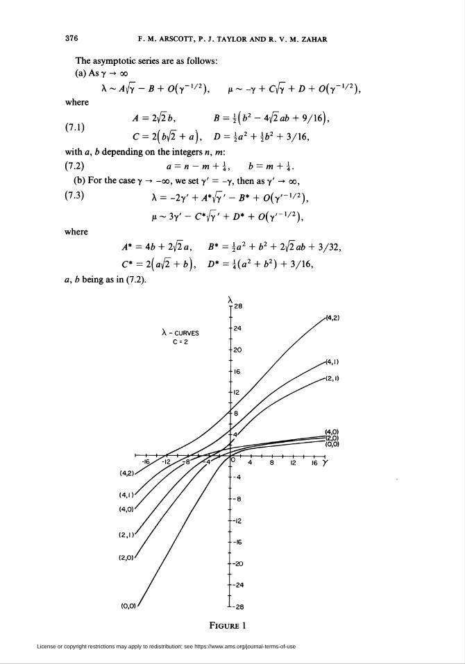
7. Results. As an indication of the results* computed by the method described

in Sections 5 and 6, we attach Figures 1 and 2 showing the first six eigenvalue

curves in the case c = 2, that is to say, for the pairs in, m) = (0,0), (1,0), (1,1),

(2,0), (2,1), (2,2). In the computations, Ay = \ was used throughout.

The corresponding values for y = 0 are

n m X p

0 0 0 0

1 0 i(3 - /3) = 0.6340 -1.5

1 1 £(3 + ]¡3) = 2.3660 -1.5

2 0 (5 - /Í3) = 1.3944 -5

2 1 5 -5

2 2 (5 +/Ï3) = 8.6054 -5

* Note. In private communication with the first author, Professor L. Fox of the Oxford University

Computing Laboratory has indicated that a two-parameter shooting method, using matrix techniques,

yields results which agree with those of the authors. He observed similar difficulties to ours in the

sensitive areas mentioned above.



(7.1)

The asymptotic series are as follows:

(a) As y -» oo

X~Af/ - B + 0(y~1/2), p~ -Y + Cyy + D + 0(y~x/1),

where

A=2]¡2b, B = {-(b2-4^2ab+ 9/16),

C = 2(bJÏ + a), D = \a2 + \b2 + 3/16,

with a, b depending on the integers n, m:

(7.2) a = n-m + \, b = m + \.

(b) For the case y -» -co, we set y' = -y, then as y' -» 00,

(7-3) X = -2y' + A*{y' - B* + 0(y'~x/2),

p ~ 3y' - C*ff' + D* + 0(y'~x/2),

where

A* = 4b + 2/2 a, B* = {a2 + b2 + 2^2 ab + 3/32,

C* = 2(aJÏ+ b), D* = Ha2 + b2) + 3/16,

a, b being as in (7.2).

X - CURVES



(4,0)

(2,0)(4,l)(4,2)|(2,l)(0,0)

p.- CURVESC = 2

(4,I)(4,0K2,I)

Figure 2

[Note. In the diagrams, the eigenvalue curves have been numbered to match the

corresponding ellipsoidal wave functions uelg, uel°, uel'2, uel°, uel'4, uel2,, the lower

index being 2n rather than «.]

8. Other Forms of the Equation; Solution by Trigonometric Series or Neumann

Series. An interesting version of the elhpsoidal wave equation, and one which may

prove computationally useful, is obtained by putting

(8.1) am z = v <=> sn z = sin v <=> t = sin2 v

in (2.1), (2.4), giving the "trigonometric form"

/o „\ /, , t ■ ■> \ d2w ,, . dw(8.2) (I — k snr v)—- - k sin vcos v —V V dv2 dv

— (a + bk2 sin2 v + qk4 sin4 v)w = 0

or, using multiple angles,

2 2(8.3) fl -\k2 + \k2coi1 2 . dw

- —ksm2v—-2 dv

iR + Scos2t) + rcos4u)w = 0,



where

R a + \bk2 + qk4, S = \k\b + qk2), T = —f-

We now seek to solve this by a trigonometric series; the form which corresponds

to a uel-function is a series of even cosines

(8-4)l_

2C°2crcos2ro.

Substitution in (8.3) yields a five-term recursion:

(8.5a)

(8.5b)

(8.5c)

Rc0 + (S- k2)cx + Tc2 = 0,

2Sc° + r+Ä-4i

+

H)S-(r-l)(r-\)k

\s-(r+l)(r + ^k

[^S-3k2 c2+2rC3 = °'

+ R l-\k2

"r+\ ' 2 r + 2 0, r>2.

The fact that we have five terms instead of four in the recursion may be

compensated by the symmetries in (8.5c). These series were first considered by

Campbell [8].

A similar analysis to that of Section 5 shows that, as r -* oo, the ratio cr+x/cr

must have one of the asymptotic forms

(8.6)2k2

-r , —1 + k'

1 -k"

1 - k'

1 + k' 2k1

and clearly the numerical treatment must be such as to pick out the solution which

has the last-mentioned behavior.

Mention should also be made of another possible mode of solution, namely the

use of Neumann series (i.e., series of Bessel functions). Such series again lead to

five-term recursion relations; details are given in [4].

9. The Other Types of Ellipsoidal Wave Function. The exposition in this paper has

concentrated on only one of the eight types of elUpsoidal wave functions, but in fact

the other seven types seem to be amenable to the same treatment.

Referring to (3.1) and (3.2), the eight types are distinguished by the eight

combinations of values 0,1 taken by p, a, t. The standard notation [2], [3] is to use

the general symbol el(z) and prefix the letters s, c, d according to the occurrence of

the extraneous factors sn z, en z, dn z in the representation (3.1) (or u, for unity, if

there are none such). Thus the eight types are written uel, sel, eel, del, seel, sdel, cdel,

scdel, with suitable suffixes.

For the purposes of this paper it is more convenient to take the solutions in the

form (3.1). By tedious working we find that the differential equation to be satisfied

by Git) has the form

(9.1) t(t - l)(t - c)G"(t) + UA2t2 - 2Axt + AQ)G'(t)

{X-X0 + (p + p0)t + yt2)Git)=0,



where the values of A2, Ax, A0, X0, p0 are as follows

Function type par A2

uel

sel

eel

del

seel

sdel

cdel

scdel

0 0 0

1 0 0

0 1 0

0 0 1

1 1 0

1 0 1

0 1 1

1 1 1

Ax A0

1 + c c

2 +2c 3c

1 +2c c

2 + c c

2 +3c 3c

3 +2c 3c

2 + 2c c

3 + 3c 3c

0

1

4C

J_4

~4+C

I +-c4

Jo + ¿)1 +c

Specifically

,42 = 2(p + a + t) + 3,

Ax = (I + p)(l +c) +T + OC,

A0 = i2p+l)c,

4X0 = ip + T)2+ip + o)2c,

4p0 = (p + o + r)(p + a + T

When Eq. (9.1) is solved formally by a series

1).

(9.2) G(t) = 2«rtr,o

then the recursion (corresponding to (5.3)) is

(9.3) yar + p + p0 + (r+ l)(r + ^/i2)

[X-X0-(r + 2)(Ax + (r + l)(l + c))]ar + 2

Mo

0

J_2

I212323

2323

+ (r + 3) ir + 2)c + ^A0 lr+i= 0.

Grateful acknowledgement is made to the Natural Sciences and Engineering

Research Council of Canada for assistance to the authors through research grants.

The authors' thanks are also expressed to the referee for a number of helpful

comments.

Department of Applied Mathematics

University of Manitoba

Winnipeg, Manitoba, Canada R3T 2N2

Department of Mathematics

University of Stirling

Stirling, Scotland

Département d'Informatique et de Recherche Operationelle

Université de Montréal

C. P. 6128, Succersale A

Montréal, P. Q., Canada H3C 3J7



1. F. M. Arscott, "Perturbation solutions of the ellipsoidal wave equation," Quart. J. Math., v. 7,

1956, pp. 161-174.

2. F. M. Arscott, "A new treatment of the ellipsoidal wave equation," Proc. London Math. Soc, v.

33, 1959, pp. 21-50.3. F. M. Arscott, Periodic Differential Equations, Pergamon Press, New York, 1964.

4. F. M. Arscott, "Neumann-series solutions of the ellipsoidal wave equation," Proc. Roy. Soc.

Edinburgh, Sect A, v. 67, 1965, pp. 69-77.5. F. M. Arscott & I. M. Khabaza, Tables of Lamé Polynomials, Pergamon Press, New York, 1962.

6. F. M. Arscott, R. Lacroix & E. T. Shymanski, "A three-term recursion and the computation of

Mathieu functions," Proc. Eighth Manitoba Conf. on Numerical Mathematics, 1978, pp. 107-115.

7. F. M. Arscott & B. D Sleeman "High-frequency approximations to ellipsoidal wave functions,"

Mathematika, v. 17, 1970, pp. 39-46.8. R. Campbell, "Sur la vibration d'un haut-parleur elliptique," C. R. Acad. Sei. Paris, v. 288, 1949,

pp. 970-972.9. W. Gautschi, "Zur Numerik rekurrenter Relationen," Computings. 9, 1972, pp. 107-126.

10. B. A. Hargrave & B. D. Sleeman, "Uniform asymptotic expansions for ellipsoidal wave

functions," J. Inst. Math. Appl., v. 14, 1974, pp. 31-40.11. G. W. Hill, "On the part of the motion of the lunar perigee," Acta. Math., v. 8, 1886, pp. 1-36.

12. E. L. Ince, Ordinary Differential Equations, Dover (Longman's), 1926.

13. E. L. Ince, "Tables of the elliptic-cylinder functions," Proc. Roy. Soc. Edinburgh, v. 52, 1932, pp.

335-423.

14. E. L. Ince, "Zeros and turning-points of the elliptic-cylinder functions," Proc. Roy. Soc. Edinburgh,

v. 52, 1932, pp. 424-433.15. E. Mathieu, "Mémoire sur le mouvement vibratoire d'une membrane de forme elliptique," J\

Math. Pures Appl., v. 13, 1868, pp. 137-203.16. R. V. M. Zahar, "A mathematical analysis of Mller's algorithm," Numer. Math., v. 27, 1977, pp.

427-447.

17. R. V. M. Zahar, "Recurrence techniques for a differential eigenvalue problem," Proc. Eighth

Manitoba Conf. on Numerical Mathematics, 1978, pp. 479-485.


Documents

On the Numerical Construction of Ellipsoidal Wave Functions