Embed Size (px)
Citation preview
On the modeling and the optimal motion planning of manipulators via a modified D* Lite search algorithm
AMIR FEIZOLLAHI and RENE V. MAYORGA
Department of Industrial Systems Engineering University of Regina
3737 Wascana Parkway, Regina, Saskatchewan CANADA
[email protected] and [email protected] Abstract: - The motion planning of the manipulators is a topic in robotics that has been studied extensively and there are many solutions available in the literature. However, the motion planning of manipulators considering the system dynamics with respect to their energy consumption level is still a challenging problem which requires a combination of interdisciplinary studies to yield an optimal solution. In this paper, a framework is developed to model the user-defined manipulator, design a motion planner implementing a proposed search algorithm, and simulate the robot motion in different environments. The superiority of the search algorithm is investigated and the development of the MATLAB framework is discussed thoroughly accompanying the simulation results. Key-Words: - Manipulator dynamics, Motion planning, Trajectory optimization, Graph search 1 Introduction Manipulation is the main or part of many industrial and daily applications that involve picking, moving and placing objects in different workspaces. Saving labor and reducing the cost of operation has been always a big challenge for the designers to minimize the time and effort needed to perform these tasks. In many applications such as working in dangerous environment [1], to dexterous manipulation [2], and inter-zonal placement in industrial workspaces [3], using human operators can be either inefficient or dangerous. Industrial robotic manipulators, as one of the main groups of robots, are designed to manipulate objects and perform tasks with minimum contact with a human.
Motion planning and developing an optimized algorithm for converting a high-level task from human to a low-level description for the robot, has been one of the most challenging problems for the programmers. Motion planning is the process of generating the best motion for the robot based on the defined criteria, restriction on the workspaces, and the robot model. This process usually involves collision-free configuration, coordinating the robot’s motion, dynamic modeling, and object manipulation [4]. Motion planning can be generally classified into two main groups: motion planning in static environment and motion planning in dynamic environment.
In static environment, the obstacles, costs, workspace features, and other required information for obtaining the optimal path are known and can be computed in the pre-processing phase. Hart et al. proposed an algorithm for dealing with this type of motion planning problem which is known as A* [5]. The A* is an heuristic search algorithm and one of the most popular algorithms having an easy implementation procedure.
The D* algorithm is an informed incremental graph search algorithm that has been widely used for the automatic navigation of the mobile robots in unknown environment [6]. The D* Lite [7] which is an incremental heuristic search algorithm, combines A* algorithm and Dynamic SWSF-FP algorithm [8] to determine the best path for the robot while the path costs change due to discovering new obstacles or changes in obstacle features.
In this paper, the development and implementation of a MATLAB framework for modeling the wide range of user-defined (industrial) manipulators and generation of a locally optimal collision free trajectory is presented.
A novel approach is applied to combine the dynamic model of the manipulator and its actuators as a unified on-line equation of motion which yields to calculation of energy consumption of the robot actuators between any two nodes with pre-defined constraints.
WSEAS TRANSACTIONS on SYSTEMS and CONTROL Amir Feizollahi, Rene V. Mayorga
E-ISSN: 2224-2856 148 Volume 12, 2017

Here, also a novel modification is proposed to the D* Lite [7] (one of the most recent search algorithms) to make it considerably faster and more efficient. The comparison between the proposed search algorithm and other widely known, like the A* [5], has been investigated and the results of implementation of the modified search algorithm are also presented correspondingly. 2 Robotic Manipulator Modeling As mentioned in the previous section, there are many research papers covering the manipulators modeling and there also lots of articles for different approaches of motion planning for the manipulators. However, combining the robot model with motion planning and including the output of the dynamic model in the motion planning procedure requires a novel methodology.
Deriving the equation of motion of the robot associated with dynamics of the manipulator and its actuating system (DC motors in this case), results in the calculation of energy consumption between any two nodes in the cost function of the search algorithm. Of course, reaching a locally optimum solution for the robot motion planning cannot be effectively done when the cost function is solely based on the kinematics of the robot.
In order to calculate the energy consumption of manipulator during its motion from the start node to the goal node, the mathematical model of the robot has to be developed. Using Hamilton’s principle [9] for conservative systems between two states, the dynamic model equation of the manipulator can be derived as Eq. (1).
( ) ( ) ( )TD q q q C q q G q τ+ + = (1)
Where D, C, and G are the inertia matrix, Christoffel matrix, and the gravity vector, respectively. The DC motors, are widely used for robot industrial application and are one of the most common actuators for the robotic and control systems. Developing the motion of equation of the motor and its circuit dynamic equation using Kirchhoff’s voltage law and combining the developed equation with Eq. (1), the uniform equation of motion of the robotic manipulator is:
1
0 1 00
( ) B0 0( ) ( )
0
t
L
e
Kd C Vdt J D J D
i iK RL L
θ θθθ θ
θ θ
+ = + + + − −
(2)
In which (Nonlinear Gravitational Terms) can be calculated using Eq. (3).
0
( )( )
0
GNGTJ D
θθ
= − +
(3)
Table 1. List of parameters and variables in the governing equation of the robot-actuator system
Name Explanation
Para
met
ers
J Rotor’s moment of inertia
B Motor viscous friction constant
Ke Electromotive force constant
Kt Motor torque constant
R Electric resistance
L Electric inductance
Var
iabl
es
Joint’s angular velocity
i Armature current
V Armature input voltage
Using the fourth order of Runge-Kutta method for solving the derived differential equation of the system gives a very consistent approximation of its behavior which is the basis of the search algorithm. More details on deriving the governing equation, Eq. (2) can be found in [10].
Dynamic Modelof The Robot
Kinematic Modelof The Robot
Path length
Heuristic Value
Energy Consumption
Cost FunctionCollision Free
AndEnergetically Optimized Path
Dynamic Modelof The Actuators
Figure 1. Cost function and the robot modeling relationship
3 Graph Traversal Search Algorithm Graph traversal algorithms deal with the problems that are expressible in terms of a search over a map of nodes in order to find all the reachable nodes, identify the best reachable nodes, and generate the best path through a network of nodes with defined constraints.
Graph search algorithms are mainly categorized under either an incremental or an heuristic search algorithm. In incremental search algorithms, the
WSEAS TRANSACTIONS on SYSTEMS and CONTROL Amir Feizollahi, Rene V. Mayorga
E-ISSN: 2224-2856 149 Volume 12, 2017
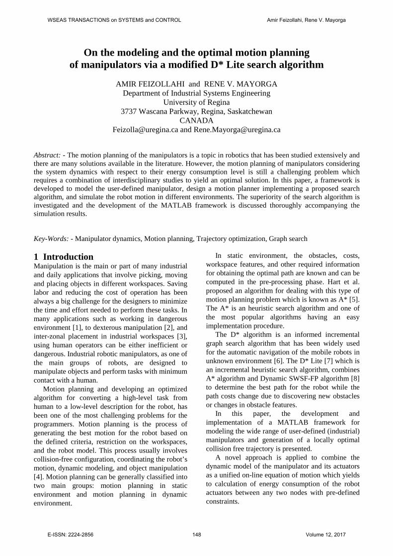
search is based on the information from the previous search information as a feed for the new search while in heuristic search algorithms the heuristic information of each node is considered to focus the search on minimizing the distance to the goal node.
Incremental heuristic search algorithms refer to the algorithms which use both incremental and heuristic search features to speed up the search while focusing on reaching the goal node.
How to use previous search results efficiently
HeuristicSearch
IncrementalSearch
Artificial Intelligence Algorithm Theory
How to search using heuristic info. to guide the search
Figure 2. Incremental heuristic algorithms foundation
As previously mentioned, this article focuses on solving of partially-known environment search problems. In this case some of the reachable nodes are known, and some of them are either unknown or some of their features change during the robot motion over the map. The D* Lite algorithm is one of the most recent and most efficient graph search algorithms for partially known environments [7]. The D* Lite is basically the incremental version of A* algorithm. D* Lite implements same navigation procedure as D* and it is at least as efficient as D*. However, D* lite procedure is much shorter and actually different than the D* algorithm.
In D* Lite two main estimates of cost are assigned to each node, g and rhs:
Table 2. Features of each node in D* Lite algorithm Feature Explanation
g the objective function value
rhs one-step look-forward of the objective function value
consistent Electromotive force constant
inconsistent Motor torque constant
Inconsistent nodes are the nodes on the “open list” with the priority of process. As a matter of fact, the key value of a node defines the priority of that node on the open list which is a combination of the g, rhs and heuristic value of the node.
Table 3. List of functions associated with the priority calculation of each node
Feature Calculation
rhs ( ) ( ) ( )( )( )min cost ,p Succ urhs u u p g p∈= +
key ( ) ( )( ) ( )( ) ( )( )
min , ,( )
min ,
g u rhs u h start ukey u
g u rhs u
+ =
The key value of a node, according to Table 3, is the summation of the heuristic value of the node, h, and the minimum of its g and rhs value. If the key value of two nodes are calculated to be exactly the same, the minimum of g and rhs values are considered to be the tie breaker.
D* Lite algorithm has five main procedures: Initialization, Main Procedure, Key Value Calculation, Node Update, and Best Path Generation [7]. Creating the open list, setting the initial value of nodes (g and rhs), inserting the goal node to the open list and setting its rhs value to zero are the programming methods of Initialization procedure. Unlike A*, the D* Lite algorithm starts the node processing from the goal node and the graph search will be terminated once the algorithm reaches the start node. The Key Value Calculation procedure is simply a function with the nodes as its input and the key value as the output. This output is later returned to the caller procedure (Figure 3).
(a)
(b)
Figure 3. (a) Initialization procedure (b) Key Value Calculation procedure
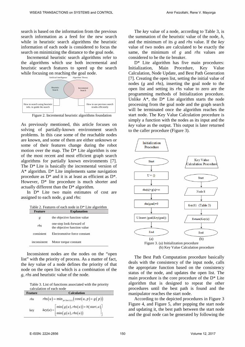
The Best Path Computation procedure basically deals with the consistency of the input node, calls the appropriate function based on the consistency status of the node, and updates the open list. The main procedure is the core procedure of the D* Lite algorithm that is designed to repeat the other procedures until the best path is found and the manipulator reaches the start node.
According to the depicted procedures in Figure 3 Figure 4, and Figure 5, after popping the start node and updating it, the best path between the start node and the goal node can be generated by following the
WSEAS TRANSACTIONS on SYSTEMS and CONTROL Amir Feizollahi, Rene V. Mayorga
E-ISSN: 2224-2856 150 Volume 12, 2017
gradient of g values from the start node. As a result, to obtain the best path, the g values of all the neighboring nodes have to be compared to each other which requires a time-consuming sorting process. A modification in generation of the best path after processing the nodes between the start node and the goal node can significantly increase the efficiency of this algorithm.
Figure 4. D* Lite Best Path Computation procedure
Figure 5. D* Lite Main procedure
By adding a function to Node Update procedure of D* Lite algorithm, the best path can be easily generated by connecting the output nodes of this
function. According to Figure 6, “Store” function saves the best neighbor node for the node that is under process. After calculating the rhs value of the input node, its best neighboring node is saved as a feature of the node. Once the search algorithm reaches the start node and the graph traversal is terminated, the best path between the start node and the goal node can be generated by adding the best neighboring nodes one after each other from the start node. This modifications totally eliminate any extra sorting process after reaching the start node. This process on a sample network of nodes is depicted in Figure 7.
U.Remove(u)
u ≠ goal
rhs(u) [Equation 2-34]
u ϵ U
Start
New Node Update Procedure
g(u)≠rhs(u)
U.Insert(u,key(u))
End
Yes
No
Yes
Yes
No
No
Store the Best Neighbour Node
Figure 6. Modification to D* Lite, Node Update procedure
ID = 3g = 2
rhs = 2
ID = 2g = 1
rhs = 1
ID = 1g = 0
rhs = 0
ID = 6g = 2.4
rhs = 2.4
ID = 5g = 1.4
rhs = 1.4
ID = 4g = ∞
rhs = ∞
ID = 9g = 2.8
rhs = 2.8
ID = 8g = 2.4
rhs = 2.4
ID = 7g = 2.8
rhs = 2.8
ID = 12g = ∞
rhs = 3.8
ID = 11g = 3.4
rhs = 3.4
ID = 10g = ∞
rhs = 3.8GO
AL
STA
RT
Figure 7. The best path between the start and the goal node
using modified D* Lite algorithm
WSEAS TRANSACTIONS on SYSTEMS and CONTROL Amir Feizollahi, Rene V. Mayorga
E-ISSN: 2224-2856 151 Volume 12, 2017
4 MATLAB Framework Development The process of robot modeling and also the theoretical procedures for the proposed search algorithm in partially-known environment were provided in the previous sections. For implementing the search algorithm on a user-defined manipulator, a MATLAB framework is designed to model the robot, implement the modified D* Lite algorithm, and simulate the robot motion in different scenarios.
The designed framework consists of a very large number of lines scripts in MATLAB with several classes, functions, and properties. The overall steps (classes) for obtaining a collision free and optimized motion planning of a user-defined manipulator are included in Table 4.
Table 4. List of MATLAB classes for modeling and implementing the search algorithm*
Class Purpose
Robot Dynamics
a class with several functions and properties for modeling the robot, developing the equations of motion
Motor Dynamics
a class for developing the equation of motion of the user-defined actuator, solving the differential equations and calculating the energy consumption
Occupancy Analysis
group of classes and sub-classes for generating random configuration of the manipulators and identifying the workspace accordingly
MPD* Lite a class that is designed to implement the proposed search algorithm and find the best path with optimized energy consumption
Robot Simulation
a class for simlating the robot miotion and generating the corresponding graphic output
*all the MATLAB scripts can be found in Appendix A of [11].
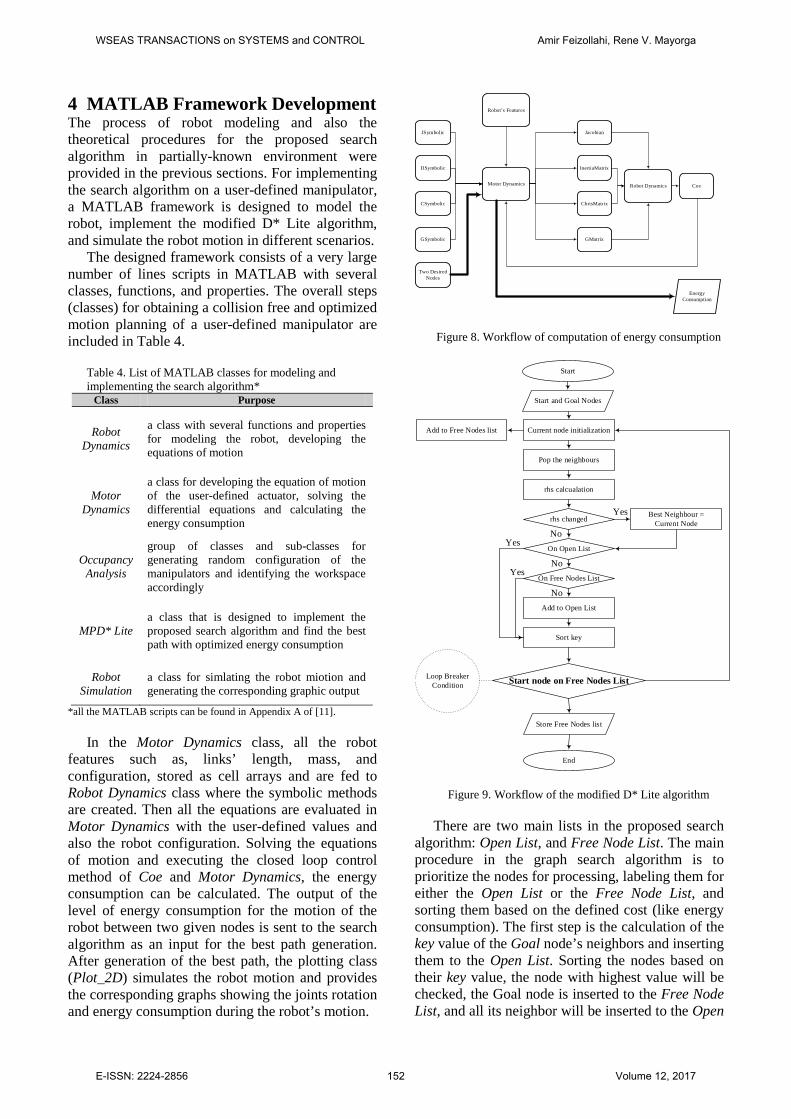
In the Motor Dynamics class, all the robot features such as, links’ length, mass, and configuration, stored as cell arrays and are fed to Robot Dynamics class where the symbolic methods are created. Then all the equations are evaluated in Motor Dynamics with the user-defined values and also the robot configuration. Solving the equations of motion and executing the closed loop control method of Coe and Motor Dynamics, the energy consumption can be calculated. The output of the level of energy consumption for the motion of the robot between two given nodes is sent to the search algorithm as an input for the best path generation. After generation of the best path, the plotting class (Plot_2D) simulates the robot motion and provides the corresponding graphs showing the joints rotation and energy consumption during the robot’s motion.
Robot Dynamics
Robot’s Features
Motor Dynamics
JacobianJSymbolic
InertiaMatrixDSymbolic
ChrisMatrixCSymbolic
GMatrixGSymbolic
Coe
Energy Consumption
Two Desired Nodes
Figure 8. Workflow of computation of energy consumption
Start and Goal Nodes
Current node initialization
Start
Pop the neighbours
rhs calcualation
rhs changed Best Neighbour = Current Node
On Open List
On Free Nodes List
Add to Open List
Sort key
Start node on Free Nodes List
Store Free Nodes list
Add to Free Nodes list
End
Loop BreakerCondition
Yes
NoYes
YesNo
No
Figure 9. Workflow of the modified D* Lite algorithm
There are two main lists in the proposed search algorithm: Open List, and Free Node List. The main procedure in the graph search algorithm is to prioritize the nodes for processing, labeling them for either the Open List or the Free Node List, and sorting them based on the defined cost (like energy consumption). The first step is the calculation of the key value of the Goal node’s neighbors and inserting them to the Open List. Sorting the nodes based on their key value, the node with highest value will be checked, the Goal node is inserted to the Free Node List, and all its neighbor will be inserted to the Open
WSEAS TRANSACTIONS on SYSTEMS and CONTROL Amir Feizollahi, Rene V. Mayorga
E-ISSN: 2224-2856 152 Volume 12, 2017
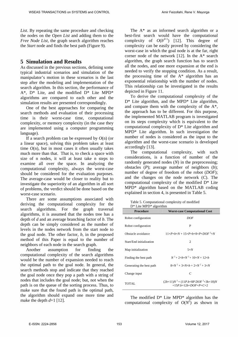
List. By repeating the same procedure and checking the nodes on the Open List and adding them to the Free Node List, the graph search algorithm reaches the Start node and finds the best path (Figure 9). 5 Simulation and Results As discussed in the previous sections, defining some typical industrial scenarios and simulation of the manipulator’s motion in these scenarios is the last step after the modeling and implementation of the search algorithm. In this section, the performance of A*, D* Lite, and the modified D* Lite MPD* algorithms are compared to each other and the simulation results are presented correspondingly.
One of the best approaches for comparing the search methods and evaluation of their processing time is their worst-case time, computational complexity, or memory complexity (in the case they are implemented using a computer programming language).
If a search problem can be expressed by O(n) (or a linear space), solving this problem takes at least time O(n), but in most cases it often usually takes much more than that. That is, to check a space with size of n nodes, it will at least take n steps to examine all over the space. In analyzing the computational complexity, always the worst-case should be considered for the evaluation purposes. The average-case would be closer to reality but to investigate the superiority of an algorithm in all sort of problems, the verdict should be done based on the worst-case scenario.
There are some assumptions associated with deriving the computational complexity for the search algorithms. For the graph traversal algorithms, it is assumed that the nodes tree has a depth of d and an average branching factor of b. The depth can be simply considered as the number of levels in the nodes network from the start node to the goal node. The other factor, b, in the proposed method of this Paper is equal to the number of neighbors of each node in the search graph.
Another assumption for finding the computational complexity of the search algorithms would be the number of expansion needed to reach the optimal path to the goal node. In general, the search methods stop and indicate that they reached the goal node once they pop a path with a string of nodes that includes the goal node; but, not when the path is on the queue of the sorting process. Thus, to make sure that the found path is the optimal path, the algorithm should expand one more time and make the depth d+1 [12].
The A* as an informed search algorithm or a best-first search would have the computational complexity of O(bd+1) [12]. This degree of complexity can be easily proved by considering the worst-case in which the goal node is at the far, right corner node of the network [12]. In the A* search algorithm, the graph search function has to search all the nodes, and one more expansion at the end is needed to verify the stopping condition. As a result, the processing time of the A* algorithm has an exponential relationship with the number of nodes. This relationship can be investigated in the results depicted in Figure 11.
To derive the computational complexity of the D* Lite algorithm, and the MPD* Lite algorithm, and compare them with the complexity of the A*, the approach has to be different. For this purpose, the implemented MATLAB program is investigated on its steps complexity which is equivalent to the computational complexity of D* Lite algorithm and MPD* Lite algorithm. In such investigation the number of nodes is considered as the input to the algorithm and the worst-case scenario is developed accordingly [13].
The computational complexity, with such considerations, is a function of number of the randomly generated nodes (N) in the preprocessing; obstacles (P); average number of neighbors (b); number of degree of freedom of the robot (DOF); and the changes on the node network (C). The computational complexity of the modified D* Lite MPD* algorithm based on the MATLAB coding explained in section 4, is presented in Table 5.
Table 5. Computational complexity of modified D* Lite MPD* algorithm
Procedure Worst-case Computational Cost
Robot configuration DOF
Robot configuration P
Obstacle avoidance 11×P×b×N + 15×P×b+8×P×DOF 2×N
Start/End initialization 2
Map initialization 5×N
Finding the best path N 2 + 2×b×N 2 + 10×N + 12×b
Generating the best path 8×N 2 + 3×N×b + 2×N 2 + 3×N
Change input C
TOTAL (2b+11)N 2 + (11P.b+8P.DOF 2+3b+18)N +15P.b+12b+DOF+P+C+2
The modified D* Lite MPD* algorithm has the
computational complexity of O(N2) as shown in
WSEAS TRANSACTIONS on SYSTEMS and CONTROL Amir Feizollahi, Rene V. Mayorga
E-ISSN: 2224-2856 153 Volume 12, 2017
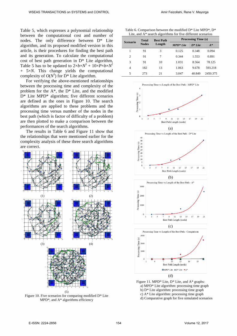
Table 5, which expresses a polynomial relationship between the computational cost and number of nodes. The only difference between D* Lite algorithm, and its proposed modified version in this article, is their procedures for finding the best path and its generation. To calculate the computational cost of best path generation in D* Lite algorithm, Table 5 has to be updated to 2×b×N3 + 10×P×b×N2 + 5×N. This change yields the computational complexity of O(N3) for D* Lite algorithm.
For verifying the above-mentioned relationships between the processing time and complexity of the problem for the A*, the D* Lite, and the modified D* Lite MPD* algorithm; five different scenarios are defined as the ones in Figure 10. The search algorithms are applied to these problems and the processing time versus number of the nodes in the best path (which is factor of difficulty of a problem) are then plotted to make a comparison between the performances of the search algorithms.
The results in Table 6 and Figure 11 show that the relationships that were mentioned earlier for the complexity analysis of these three search algorithms are correct.
0 1 2 3 4 5 6 7 8 9 100
1
2
3
4
5
6
7
8
9
10
12
3
4
5
6
7
8
910
11
12
13
14
15
16
17
18
19
20
21
22
23
24
25
26
27
28
29
30
31
32
33
3435
36
37
38
3940
41
42
43
44
45
46
47
48
49
50
51
52
53
54
55
56
57
58
59
60
61
62
63
64
65
66
67
68
69
70
71
72
73
74
75
76
77
78
79
80
8182
83
8485
86
87
88
89
90
91
x
y
(1)
0 1 2 3 4 5 6 7 8 9 100
1
2
3
4
5
6
7
8
9
10
12
3
4
56
7
8
910
11
12
13
14
15
16
17
18
19
20
21
22
23
24
25
26
27
28
29
30
31
32
33
3435
36
37
38
3940
41
42
43
44
45
46
47
48
49
50
51
52
53
54
55
56
57
58
59
60
61
62
63
64
65
66
67
68
69
70
71
72
73
74
75
76
77
78
79
80
8182
83
8485
86
87
88
89
90
91
x
y
(2)
0 1 2 3 4 5 6 7 8 9 100
1
2
3
4
5
6
7
8
9
10
12
3
4
56
7
8
910
11
12
13
14
15
16
17
18
19
20
21
22
23
24
25
26
27
28
29
30
31
32
33
3435
36
37
38
3940
41
42
43
44
45
46
47
48
49
50
51
52
53
54
55
56
57
58
59
60
61
62
63
64
65
66
67
68
69
70
71
72
73
74
75
76
77
78
79
80
8182
83
8485
86
87
88
89
90
91
x
y
(3)
0 1 2 3 4 5 6 7 8 9 100
1
2
3
4
5
6
7
8
9
10
12
3
4
56
7
8
910
11
12
13
14
15
16
17
18
19
20
21
22
23
24
25
26
27
28
29
30
31
32
33
34
35
3637
38
39
4041
42
43
44
4546
47
48
49
50
51
52
53
54
55
56
57
58
59
60
61
62
63
64
65
66
67
68
69
70
71
72
73
74
75
76
77
78
79
80
8182
83
84
85
86
87
8889
90
91
92
93
94
95
96
9798
99
100
101
102
103
104
105
106
107
108
109
110
111
112
113
114
115 116
117
118
119
120
121
122123
124 125
126
127
128
129
130
131
132
133
134
135
136
137138
139
140
141
142
143
144
145
146
147
148
149
150
151
152
153
154
155156
157
158
159
160
161
162
163
164
165
166
167
168
169
170
171
172
173
174
175
176
177
178
179
180
181
182
x
y
(4)
0 1 2 3 4 5 6 7 8 9 100
1
2
3
4
5
6
7
8
9
10
12
3
4
56
7
8
910
11
12
13
14
15
16
17
18
19
20
21
22
23
24
25
26
27
28
29
30
31
32
33
34
3536
37
38
39
40
41
42
4344
45
46
47
48
49
50
51
52
53
54
55
56
57
58
59
60
61
62
63
64
65
66
67
68
69
70
71
72
73
74
75
76
77
78
79
80
81
82
83
84
8586
87
88
89
90
91
92
93
9495
96
97
98
99100
101
102
103
104
105
106
107
108
109
110
111
112
113
114
115
116 117
118
119
120
121
122123
124
125126
127
128
129
130
131
132
133
134
135
136
137
138
139
140
141
142
143
144
145
146
147
148
149
150
151
152
153
154
155
156
157
158
159
160
161
162
163
164
165
166
167
168
169
170
171
172
173
174
175
176
177178
179
180
181
182
183
184
185
186
187
188
189
190
191
192
193
194
195
196
197
198
199
200
201
202
203
204
205
206
207
208
209
210 211
212
213
214
215
216
217
218
219
220
221
222
223
224
225
226
227
228
229
230
231
232
233
234
235
236
237
238
239
240
241242
243
244
245
246
247
248
249
250
251
252
253
254
255
256
257
258
259
260
261
262
263
264
265
266
267268
269
270
271
272
273
x
y
(5)
Figure 10. Five scenarios for comparing modified D* Lite MPD*, and A* algorithms efficiency
Table 6. Comparison between the modified D* Lite MPD*, D* Lite, and A* search algorithms for five different scenarios
Scenario Total Nodes
Best Path Length
Processing Time (s)
MPD* Lite D* Lite A*
1 91 3 0.125 0.348 0.094
2 91 7 0.344 1.553 0.891
3 91 10 1.031 8.564 78.125
4 182 13 1.063 9.678 593.218
5 273 21 3.047 40.849 2450.375
(a)
(b)
(c)
(d)
Figure 11. MPD* Lite, D* Lite, and A* graphs: a) MPD* Lite algorithm: processing time graph b) D* Lite algorithm: processing time graph c) A* Lite algorithm: processing time graph d) Comparative graph for five simulated scenarios
WSEAS TRANSACTIONS on SYSTEMS and CONTROL Amir Feizollahi, Rene V. Mayorga
E-ISSN: 2224-2856 154 Volume 12, 2017
In the following section, the modeling and motion planning of the manipulators based on the energy consumption in typical industrial problems are discussed. The simulation parameters for modeling the DC motors are presented in Table 7.
Table 7. Simulation parameters of robot’s actuators Parameter Description Value
R Electric resistance 1 Ω
L Electric inductance 0.5 H
tK Motor torque constant 10.01 . .N m Amp−
eK Electromotive force constant 1 10.02 . .V rad s− −
b Motor viscous friction constant 0.1 . .N m s
pK PD-Control gain constant 0.1 . .N m s
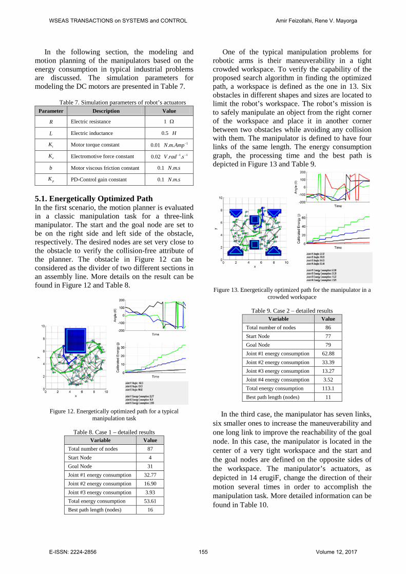
5.1. Energetically Optimized Path In the first scenario, the motion planner is evaluated in a classic manipulation task for a three-link manipulator. The start and the goal node are set to be on the right side and left side of the obstacle, respectively. The desired nodes are set very close to the obstacle to verify the collision-free attribute of the planner. The obstacle in Figure 12 can be considered as the divider of two different sections in an assembly line. More details on the result can be found in Figure 12 and Table 8.
Figure 12. Energetically optimized path for a typical
manipulation task
Table 8. Case 1 – detailed results Variable Value
Total number of nodes 87 Start Node 4 Goal Node 31 Joint #1 energy consumption 32.77 Joint #2 energy consumption 16.90 Joint #3 energy consumption 3.93 Total energy consumption 53.61 Best path length (nodes) 16
One of the typical manipulation problems for robotic arms is their maneuverability in a tight crowded workspace. To verify the capability of the proposed search algorithm in finding the optimized path, a workspace is defined as the one in 13. Six obstacles in different shapes and sizes are located to limit the robot’s workspace. The robot’s mission is to safely manipulate an object from the right corner of the workspace and place it in another corner between two obstacles while avoiding any collision with them. The manipulator is defined to have four links of the same length. The energy consumption graph, the processing time and the best path is depicted in Figure 13 and Table 9.
Figure 13. Energetically optimized path for the manipulator in a
crowded workspace
Table 9. Case 2 – detailed results Variable Value
Total number of nodes 86 Start Node 77 Goal Node 79 Joint #1 energy consumption 62.88 Joint #2 energy consumption 33.39 Joint #3 energy consumption 13.27 Joint #4 energy consumption 3.52 Total energy consumption 113.1 Best path length (nodes) 11
In the third case, the manipulator has seven links, six smaller ones to increase the maneuverability and one long link to improve the reachability of the goal node. In this case, the manipulator is located in the center of a very tight workspace and the start and the goal nodes are defined on the opposite sides of the workspace. The manipulator’s actuators, as depicted in erugiF14 , change the direction of their motion several times in order to accomplish the manipulation task. More detailed information can be found in Table 10.
WSEAS TRANSACTIONS on SYSTEMS and CONTROL Amir Feizollahi, Rene V. Mayorga
E-ISSN: 2224-2856 155 Volume 12, 2017
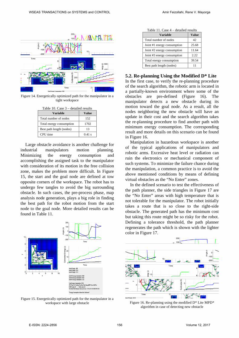
Figure 14. Energetically optimized path for the manipulator in a
tight workspace
Table 10. Case 3 – detailed results Variable Value
Total number of nodes 152
Total energy consumption 1702 Best path length (nodes) 13
CPU time 0.41 s
Large obstacle avoidance is another challenge for industrial manipulators motion planning. Minimizing the energy consumption and accomplishing the assigned task to the manipulator with consideration of its motion in the free collision zone, makes the problem more difficult. In Figure 15, the start and the goal node are defined at tow opposite corners of the workspace. The robot has to undergo few tangles to avoid the big surrounding obstacle. In such cases, the pre-process phase, map analysis node generation, plays a big role in finding the best path for the robot motion from the start node to the goal node. More detailed results can be found in Table 11.
Figure 15. Energetically optimized path for the manipulator in a
workspace with large obstacle
Table 11. Case 4 – detailed results Variable Value
Total number of nodes 42 Joint #1 energy consumption 25.68 Joint #2 energy consumption 11.64 Joint #3 energy consumption 2.22 Total energy consumption 39.54 Best path length (nodes) 11
5.2. Re-planning Using the Modified D* Lite In the first case, to verify the re-planning procedure of the search algorithm, the robotic arm is located in a partially-known environment where some of the obstacles are pre-defined (Figure 16). The manipulator detects a new obstacle during its motion toward the goal node. As a result, all the nodes neighboring the new obstacle will have an update in their cost and the search algorithm takes the re-planning procedure to find another path with minimum energy consumption. The corresponding result and more details on this scenario can be found in Figure 16.
Manipulation in hazardous workspace is another of the typical applications of manipulators and robotic arms. Excessive heat level or radiation can ruin the electronics or mechanical component of such systems. To minimize the failure chance during the manipulation, a common practice is to avoid the above mentioned conditions by means of defining virtual obstacles as the “No Enter” zones.
In the defined scenario to test the effectiveness of the path planner, the side triangles in Figure 17 are the “No Enter” areas with high temperature that is not tolerable for the manipulator. The robot initially takes a route that is so close to the right-side obstacle. The generated path has the minimum cost but taking this route might be so risky for the robot. Defining a tolerance threshold, the path planner regenerates the path which is shown with the lighter color in Figure 17.
Figure 16. Re-planning using the modified D* Lite MPD*
algorithm in case of detecting new obstacle
WSEAS TRANSACTIONS on SYSTEMS and CONTROL Amir Feizollahi, Rene V. Mayorga
E-ISSN: 2224-2856 156 Volume 12, 2017
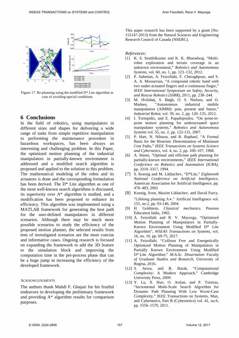
Figure 17. Re-planning using the modified D* Lite algorithm in
case of avoiding special conditions
6 Conclusions In the field of robotics, using manipulators in different sizes and shapes for delivering a wide range of tasks from simple repetitive manipulation to performing the maintenance procedure in hazardous workspaces, has been always an interesting and challenging problem. In this Paper, the optimized motion planning of the industrial manipulators in partially-known environment is addressed and a modified search algorithm is proposed and applied to the solution to this problem. The mathematical modeling of the robot and its actuators is done and the corresponding formulation has been derived. The D* Lite algorithm as one of the most well-known search algorithms is discussed, its superiority over A* algorithm is studied, and a modification has been proposed to enhance its efficiency. This algorithm was implemented using a MATLAB framework for generating the best path for the user-defined manipulators in different scenarios. Although there may be much more possible scenarios to study the efficiency of the proposed motion planner, the selected results from tens of investigated scenarios are the most concise and informative cases. Ongoing research is focused on expanding the framework to add the 3D feature to the simulation block and improving the computation time in the pre-process phase that can be a huge jump in increasing the efficiency of the developed framework. ACKNOWLEDGMENTS The authors thank Mahdi F. Ghajari for his fruitful endeavors in developing the preliminary framework and providing A* algorithm results for comparison purposes.
This paper research has been supported by a grant (No: 155147-2013) from the Natural Sciences and Engineering Research Council of Canada (NSERC).
References: [1] K. S. Senthilkumar and K. K. Bharadwaj, “Multi-
robot exploration and terrain coverage in an unknown environment,” Robotics and Autonomous Systems, vol. 60, no. 1, pp. 123–132, 2012.
[2] P. Sabetian, A. Feizollahi, F. Cheraghpour, and S. A. A. Moosavian, “A compound robotic hand with two under-actuated fingers and a continuous finger,” IEEE International Symposium on Safety, Security, and Rescue Robotics (SSRR), 2011, pp. 238–244.
[3] M. Hvilshøj, S. Bøgh, O. S. Nielsen, and O. Madsen, “Autonomous industrial mobile manipulation (AIMM): past, present and future,” Industrial Robot, vol. 39, no. 2, pp. 120–135, 2012.
[4] I. Tortopidis, and E. Papadopoulos. “On point-to-point motion planning for underactuated space manipulator systems,” Robotics and Autonomous Systems vol. 55, no. 2, pp. 122-131, 2007.
[5] P. Hart, N. Nilsson, and B. Raphael, “A Formal Basis for the Heuristic Determination of Minimum Cost Paths,” IEEE Transactions on Systems Science and Cybernetics, vol. 4, no. 2, pp. 100–107, 1968.
[6] A. Stentz, “Optimal and efficient path planning for partially-known environments,” IEEE International Conference on Robotics and Automation (ICRA), pp. 3310–3317, 1994.
[7] S. Koenig and M. Likhachev, “D*Lite,” Eighteenth National Conference on Artificial Intelligence, American Association for Artificial Intelligence, pp. 476–483, 2002
[8] Koenig, Sven, Maxim Likhachev, and David Furcy. "Lifelong planning A∗." Artificial Intelligence vol. 155, no.2, pp. 93-146, 2004.
[9] H. Goldstein, Classical mechanics. Pearson Education India, 1965.
[10] A. Feizollahi and R. V. Mayorga, “Optimized Motion Planning of Manipulators in Partially-Known Environment Using Modified D* Lite Algorithm”, WSEAS Transactions on Systems, vol. 16, no. 10, pp. 69-75, 2017.
[11] A. Feizollahi. “Collison Free and Energetically Optimized Motion Planning of Manipulators in Partially Known Environment Using Modified D* Lite Algorithm;” M.A.Sc. Dissertation Faculty of Graduate Studies and Research, University of Regina, 2016.
[12] S. Arora, and B. Barak, “Computational Complexity: A Modern Approach,” Cambridge University Press, 2009.
[13] Y. Lu, X. Huo, O. Arslan, and P. Tsiotras, “Incremental Multi-Scale Search Algorithm for Dynamic Path Planning With Low Worst-Case Complexity,” IEEE Transactions on Systems, Man, and Cybernetics, Part B (Cybernetics) vol. 41, no.6, pp. 1556–1570, 2011.
WSEAS TRANSACTIONS on SYSTEMS and CONTROL Amir Feizollahi, Rene V. Mayorga
E-ISSN: 2224-2856 157 Volume 12, 2017