On the Mathematical Foundations of Theoretical Statisticschen418/study_research/Fisher1921-on the... · On the Mathematical Foundations of Theoretical Statistics Author(s): R. A

On the Mathematical Foundations of Theoretical StatisticsAuthor(s): R. A. FisherSource: Philosophical Transactions of the Royal Society of London. Series A, Containing Papersof a Mathematical or Physical Character, Vol. 222 (1922), pp. 309-368Published by: The Royal SocietyStable URL: http://www.jstor.org/stable/91208Accessed: 22/01/2010 20:17

Your use of the JSTOR archive indicates your acceptance of JSTOR's Terms and Conditions of Use, available athttp://www.jstor.org/page/info/about/policies/terms.jsp. JSTOR's Terms and Conditions of Use provides, in part, that unlessyou have obtained prior permission, you may not download an entire issue of a journal or multiple copies of articles, and youmay use content in the JSTOR archive only for your personal, non-commercial use.

Please contact the publisher regarding any further use of this work. Publisher contact information may be obtained athttp://www.jstor.org/action/showPublisher?publisherCode=rsl.

Each copy of any part of a JSTOR transmission must contain the same copyright notice that appears on the screen or printedpage of such transmission.

JSTOR is a not-for-profit service that helps scholars, researchers, and students discover, use, and build upon a wide range ofcontent in a trusted digital archive. We use information technology and tools to increase productivity and facilitate new formsof scholarship. For more information about JSTOR, please contact [email protected].

The Royal Society is collaborating with JSTOR to digitize, preserve and extend access to PhilosophicalTransactions of the Royal Society of London. Series A, Containing Papers of a Mathematical or PhysicalCharacter.

http://www.jstor.org

http://www.jstor.org/stable/91208?origin=JSTOR-pdf

http://www.jstor.org/page/info/about/policies/terms.jsp

http://www.jstor.org/action/showPublisher?publisherCode=rsl

[ 309 ]

IX. On the illathematical Foundations of Theoretical Statistics.

1By R. A. FISHER, M.A., Fellow of Gonville and Caims College, Cambridge, Chief Statistician, Rothamsted Experimental Station, Harpenden.

Communicated by DR. E. J. RUSSELL, F.R.S.

Received June 25,--Read November 17, 1921.

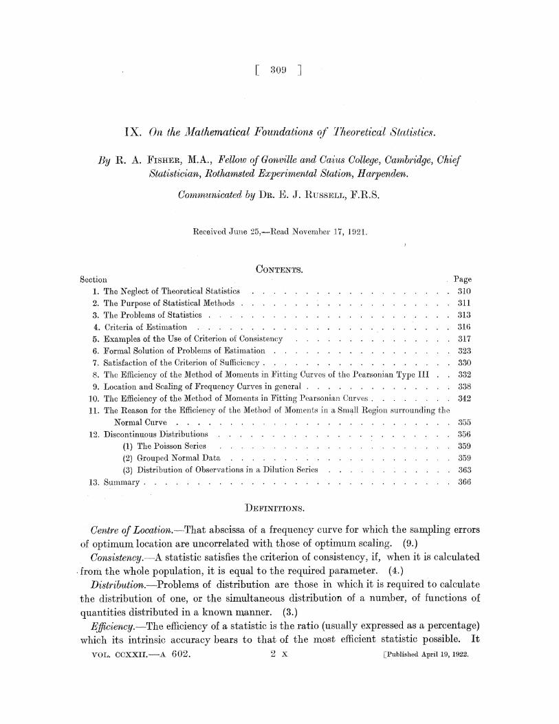
CONTENTS. Section Page

1. The Neglect of Theoretical Statistics . . . . . . . . . . . . . .. . 310

2. The Purpose of Statistical Methods ....... . . ....... 311

3. The Problems of Statistics ..................... . 313

4. Criteria of Estimation .. . . ................ . 316

5. Examples of the Use of Criterion of Consistency ... ........ . 317

6. Formal Solution of Problems of Estimation .. . ......... . 323

7. Satisfaction of the Criterion of Sufficiency ........ . . .... . 330

8. The Efficiency of the Method of Moments in Fitting Curves of the Pearsonian Type I . . 332

9. Location and Scaling of Frequency Curves in general .......... .... 338

10. The Efficiency of the Method of Moments in Fitting Pearsonian Curves . . . . . . . . 342

11. The Reason for the Efficiency of the Method of Mom.ents in a Simall Region surrounding the

Normal Curve .. . .................. 355

12. Discontinuous Distributions . . . . . . . . . . . . . . . . . . . . . 356

(1) The Poisson Series . . .. . . . . . . . . . . . . . .. . 359

(2) Grouped Normal Data . . ............ . . 359

(3) Distribution of Observations in a Dilution Series .. . 363

13. Summary .................. 366

DEFINITIONS.

Centre of Location.--That abscissa of a frequency curve for which the sampling errors of optimum location are uncorrelated with those of optimum scaling. (9.)

Consistency.-A statistic satisfies the criterion of consistency, if, when it is calculated

from the whole population, it is equal to the required parameter. (4.) Distribution.-Problems of distribution are those in which it is required to calculate

the distribution of one, or the sirmultaneous distribution of a number, of functions of

quantities distributed in a known manner. (3.) Eficiency.-The efficiency of a statistic is the ratio (usually expressed as a percentage)

which its intrinsic accuracy bears to that of the most efficient statistic possible. It VOL. CCXXII.--A 602. 2 X [Published April 19, 1922.

IMR. R. A. FISHER ON THE MATHEMATICAL

expresses the proportion of the total available relevant information of which that statistic makes use. (4 and 10.)

Efficiency (Criterion).-The criterion of efficiency is satisfied by those statistics which, when derived from large samples, tend to a normal distribution with the least possible standard deviation. (4.)

Estimation.-Problems of estimation are those in which it is required to estimate the value of one or more of the population parameters from a random sample of the

population. (3.) Intrinsic Accuracy.-The intrinsic accuracy of an error curve is the weight in large

samples, divided by the number in the sample, of that statistic of location which satisfies the criterion of sufficiency. (9.)

Isostatistical Regions.-If each sample be represented in a generalized space of which the observations are the co-ordinates, then any region throughout which any set of statistics have identical values is termed an isostatistical region.

Likelihood.-The likelihood that any parameter (or set of parameters) should have

any assigned value (or set of values) is proportional to the probability that if this were so, the totality of observations should be that observed.

Location.-The location of a frequency distribution of known form and scale is the process of estimation of its position with respect to each of the several variates. (8.)

Optimum.-The optimum value of any parameter (or set of parameters) is that value (or set of values) of which the likelihood is greatest. (6.)

Scaling.-The scaling of a frequency distribution of known form is the process of estimation of the magnitudes of the deviations of each of the several variates. (8.)

Specification.-Problems of specification are those in which it is required to specify the mathematical form of the distribution of the hypothetical population from which a sample is to be regarded as drawn. (3.)

Sufficiency.-A statistic satisfies the criterion.of sufficiency when no other statistic which can be calculated from the same sample provides any additional information as to the value of the parameter to be estimated. (4.)

Validity.-The region of validity of a statistic is the region comprised within its contour of zero efficiency. (10.)

1. THE NEGLECT OF THEORETICAL STATISTICS.

SEVERAL reasons have contributed to the prolonged neglect into which the study of

statistics, in its theoretical aspects, has fallen. In spite of the immense amount of fruitful labour which has been expended in its practical applications, the basic principles of this organ of science are still in a state of obscurity, and it cannot be denied that, during the recent rapid development of practical methods, fundamental problems have been ignored and fundamental paradoxes left unresolved. This anomalous state of statistical science is strikingly exemplified by a recent paper (1) entitled " The Funda-

310

FOUNDATIONS OF THEORETICAL STATISTICS.

mental Problem of Practical Statistics," in which one of the most eminent of modern statisticians presents what purports to be a general proof of BAYES' postulate, a proof which, in the opinion of a second statistician of equal eminence, " seems to rest upon a very peculiar-not to say hardly supposable-relation." (2.)

Leaving aside the specific question here cited, to which we shall recur, the obscurity which envelops the theoretical bases of statistical methods may perhaps be ascribed to two considerations. In the first place, it appears to be widely thought, or rather felt, that in a subject in which all results are liable to greater or smaller errors, precise definition of ideas or concepts is, if not impossible, at least not a practical necessity. In the second place, it has happened that in statistics a purely verbal confusion has hindered the distinct formulation of statistical problems; for it is customary to apply the same name, mean, standard deviation, correlation coefficient, etc., both to the true value which we should like to know,. but can only estimate, and to the particular value at which we happen to arrive by our methods of estimation; so also in applying the term probable error, writers sometimes would appear to suggest that the former quantity, and not merely the latter, is subject to error.

It is this last confusion, in the writer's opinion, more than any other, which has led to the survival to the present day of the fundamental paradox of inverse probability, which like an impenetrable jungle arrests progress towards precision of statistical concepts. The criticisms of BOOLE, VENN, and CHRYSTAL have done something towards

banishing the rnethod, at least from the elementary text-books of Algebra ; but though we may agree wholly with CHRYSTAL that inverse probability is a mistake (perhaps the only mistake to which the mathematical world has so deeply committed itself), there yet remains the feeling that such a mistake would not have captivated the minds of LAPLACE and POISSON if there had been nothing in it but error.

2. THE PURPOSE OF STATISTICAL METHODS.

In order to arrive at a distinct formulation of statistical problems, it is necessary to define the task which the statistician sets himself: briefly, and in its most concrete form, the object of statistical methods is the reduction of data. A quantity of data, which usually by its mere bulk is incapable of entering the mind, is to be replaced by relatively few quantities which shall adequately represent the whole, or which, in other words, shall contain as much as possible, ideally the whole, of the relevant information contained in the original data.

This object is accomplished by constructing a hypothetical infinite population, of which the actual data are regarded as constituting a random sample. The law of distribution of this hypothetical population is specified by relatively few parameters, which are sufficient to describe it exhaustively in respect of all qualities under discussion. Any information given by the sample, wvhich is of use in estimating the values of these parameters, is relevant information. Since the number of independent facts supplied in

2 X 2

311

MRR. . . FISIIER ON THE MATHEMATICAL

the data is usually far greater than the nunmber of facts sought, much of the information

supplied by any actual sample is irrelevant. It is the object of the statistical processes employed in the reduction of data to exclude this irrelevant information, and to isolate the whole of the relevant information contained in the data.

When we speak of the probability of a certain object fulfilling a certain condition, we

imagine all such objects to be divided into two classes, according as they do or do not fulfil the condition. This is the only characteristic in them of which we take cognisance. For this reason probability is the most elementary of statistical concepts. It is a parameter which specifies a simple dichotomy in an infinite hypothetical population, and it

represents neither more nor less than the frequency ratio which we imagine such a

population to exhibit. For example, when we say that the probability of throwing a five with a die is one-sixth, we must not be taken to mean that of any six throws with that die one and one only will necessarily be a five; or that of any six million throws, exactly one million will be fives; but that of a hypothetical population of an infinite number of throws, with the die in its original condition, exactly one-sixth will be fives. Our statement will not then contain any false assumption about the actual die, as that it will not wear out with continued use, or any notion of approximation, as in estimating the probability from a finite sample, although this notion may be logically developed once the meaning of probability is apprehended.

The concept of a discontinuous frequency distribution is merely an extension of that of a simple dichotomy, for though the number of classes into which the population is divided may be infinite, yet the frequency in each class bears a finite ratio to that of the whole population. In frequency curves, however, a second infinity is introduced. No finite sample has a frequency curve : a finite sample may be represented by a histogram, or by a frequency polygon, which to the eye more and more resembles a curve, as the size of the sample is increased. To reach a true curve, not only would an infinite number of individuals have to be placed in each class, but the number of classes (arrays) into which the population is divided must be made infinite. Consequently, it should be clear that the concept of a frequency curve includes that of a hypothetical infinite

population, distributed according to a mathematical law, represented by the curve. This law is specified by assigning to each element of the abscissa the corresponding element of probability. Thus, in the case of the normal distribution, the probability of an observation falling in the range dx, is

1 (r-mw)' __ e 22 d.x,

7V 27r

in which expression x is the value of the variate, while m, the mean, and o, the standard deviation, are the two parameters by which the hypothetical population is specified. If a sample of n be taken from such a population, the data comprise n independent facts. The statistical process of the reduction of these data is designed to extract from them all relevant information respecting the values of m and a, and to reject all other information as irrelevant.

312

FOUNDATIONS OF TtEOTRETICAL STATISTICS.

It should be noted that there is no falsehood in interpreting any set of independent measurements as a random sample from an infinite population; foi any such set of numbers are a random sample from the totality of numbers produced by the same matrix of causal conditions: the hypothetical population which we are studying is an

aspect of the totality of the effects of these conditions, of whlatever nature they may be. The postulate of randomness thus resolves itself into the question, " Of what population is this a random sample ? "which must frequently be asked by every practical statistician.

It will be seen from the above examples that the process of the reduction of data is, even in the simplest cases, performed by interpreting the available observations as a

sample from a hypothetical infinite population; this is a fortiori the case when we have more than one variate, as when we are seeking the values of coefficients of correlation. There is one point, however, which may be briefly mentioned here in advance, as it has been the cause of some confusion. In the example of the frequency curve mentioned above, we took it for granted that the values of both the mean and the standard deviation of the population were relevant to the inquiry. This is often the case, but it sometimes

happens that only one of these quantities, for example the standard deviation, is required for discussion. In the same way an infinite normal population of two correlated variates will usually require five parameters for its specification, the two means, the two standard deviations, and the correlation; of these often only the correlation is required, or if not alone of interest, it is discussed without reference to the other four quantities. In such cases an alteration has been made in what is, and what is not, relevant, and it is not

surprising that certain small corrections should appear, or not, according as the other

parameters of the hypothetical surface are or are not deemed relevant. Even more

clearly is this discrepancy shown when, as in the treatment of such. fourfold tables- as exhibit the recovery from smallpox of vaccinated and unvaccinated patients, the method of one school of statisticians treats the proportion of vaccinated as relevant, while others dismiss it as irrelevant to the inquiry. (3.)

3. THE PROBLEMS OF STATISTICS.

The problems which arise in reduction of data may be conveniently divided into three

types :

(1) Problems of Specification. These arise in the choice of the mathematical form of the population.

(2) Problems of Estimation. These involve the choice of methods of calculating from a sample statistical derivates, or as we shall call them statistics, whicl are designed to estimate the values of the parameters of the hypothetical population.

(3) Problems of Distribution. These include discussions of the distribution of statistics derived from samples, or in general any functions of quantities whose distribution is knowln.

It will be clear that when we know (1) what parameters are required to specify the

313

314 MR. R. A. FISHER ON THE MATHEMATICAL

population from which the sample is drawn, (2) how best to calculate from the sample estimates of these parameters, and (3) the exact form of the distribution, in different samples, of our derived statistics, then the theoretical aspect of the treatment of any particular body of data has been completely elucidated.

As regards problems of specification, these are entirely a matter for the practical statistician, for those cases where the qualitative nature of the hypothetical population is known do not involve any problems of this type. In other cases we may know by experience what forms are likely to be suitable, and the adequacy of our choice may be tested a posteriori. We must confine ourselves to those forms which we know how to handle, or for which any tables which may be necessary have been constructed. More or less elaborate forms will be suitable according to the volume of the data. Evidently these are considerations the nature of which may change greatly during the work of a single generation. We may instance the development by PEARSON of a very extensive system of skew curves, the elaboration of a method of calculating their parameters, and the preparation of the necessary tables, a body of work which has enormously extended the power of modern statistical practice, and which has been, by pertinacity and inspiration alike, practically the work of a single man. Nor is the introduction of the Pearsonian system of frequency curves the only contribution which their author has made to the solution of problems of specification: of even greater importance is the introduction of an objective criterion of goodness of fit. For empirical as the specification of the hypothetical population may be, this empiricism is cleared of its dangers if we can apply a rigorous and objective test of the adequacy with which the proposed population represents the whole of the available facts. Once a statistic, suitable for

applying such a test, has been chosen, the exact form of its distribution in random

samples must be investigated, in order that we may evaluate the probability that a worse fit should be obtained from a random sample of a population of the type considered. The possibility of developing complete and self-contained tests of goodness of fit deserves very careful consideration, since therein lies our justification for the free use which is made of empirical frequency formulae. Problems of distribution of great mathematical difficulty have to be faced in this direction.

Although problems of estimation and of distribution may be studied separately, they are intimately related in the development of statistical methods. Logically problems of distribution should have prior consideration, for the study of the random distribution of different suggested statistics, derived from samples of a given size, must guide us in the choice of which statistic it is most profitable to calculate. The fact is, however, that

very little progress has been made in the study of the distribution of statistics derived from. samples. In 1900 PEARSON (15) gave the exact form of the distribution of x2, the Pearsonian test of goodness of fit, and in 1915 the same author published (18) a similar result of more general scope, valid when the observations are regarded as subject to linear constraints. By an easy adaptation (17) the tables of probability derived from this formula may be made available for the more numerous cases in which linear con-


straiilt-s are imposed upon -tlhe hlypothetical population by the means which we employ in its reconstruction. The distributiori of the mean of samples of n from a normal

population has long been known, but in 1908 "Student :' (4) broke new ground by calculating the distribution of the ratio which the deviation of the mean from its population value bears to the standard deviation calculated from the sample. At the same time he gave the exact form of the distribution in samples of the standard deviation. In 1915 FISHER (5) published the curve of distribution of the correlation coefficient for the standard method of calculation, and in 1921 (6) he published the corresponding series of curves for intraclass correlations. The brevity of this list is emphasised by the absence of investigation of other important statistics, such as the regression coefficients, multiple correlations, and the correlation ratio. A formula for the probable error of any statistic is, of course, a practical necessity, if that statistic is to be of service: and in the majority of cases such formuloe have been found, chiefly by the labours of PEARSON

and his school, by a first approximation, which describes the distribution with sufficient

accuracy if the sample is sufficiently large. Problems of distribution, other than the distribution of statistics, used to be not uncommon as examination problems in probability, and the physical importance of problems of this type may be exemplified by the chemical laws of mass action, by the statistical mechanics of GIBBS, developed by JEANS in its application to the theory of gases, by the electron theory of LORENTZ, and

by PIANCK'S development of the theory of quanta, although in all these applications the methods employed have been, from the statistical point of view, relatively

simple. The discussions of theoretical statistics may be regarded as alternating between

problems of estimation and problems of distribution. In the first place a method of

calculating one of the population parameters is devised from common-sense considerations : we next require to know its probable error, and therefore an approximate solution of the distribution, in samples, of the statistic calculated. It may then become apparent that other statistics may be used as estimates of the same parameter. When the

probable errors of these statistics are compared, it is usually found that, in large samples, one particular method of calculation gives a result less subject to random errors than those given by other methods of calculation. Attacking the problem more thoroughly, and calculating the surface of distribution of any two statistics, we may find that the whole of the relevant information contained in one is contained in the other: or, in other words, that when once we know the other, knowledge of the first gives us no further information as to the value of the parameter. Finally it may be possible to

prove, as in the case of the Mean Square Error, derived from a sample of normal population (7), that a particular statistic summarises the whole of the information relevant to the corresponding parameter, which the sample contains. In such a case the problem of estimation is completely solved.

31 5

AIR. R. A. FISHER ON THE MATHEMATICAL

4. CRITERIA OF ESTIMATION.

The common-sense criterion employed in problems of estimation nlay be stated thus :- That when applied to the whole population the derived statistic should be equal to the parameter. This may be called the Criterion of Consistency. It is often the only test

applied: thus, in estimating the standard deviation of a normally distributed population, from an ungrouped sample, either of the two statistics-

= n A S (Ix- |) (Mean error)

and

,2 = S/ (x-P)2 (Mean square error) n

will lead to the correct value, r , when calculated from the whole population. They both thus satisfy the criterion of consistency, and this has led many computers to use the first formula, although the result of the second has 14 per cent. greater weight (7), and the labour of increasing the number of observations by 14 per cent. can seldom be less than that of applying the more accurate formula.

Consideration of the above example will suggest a second criterion, namely :-That in large samples, when the distributions of the statistics tend to normality, that statistic is to be chosen which has the least probable error.

This may be called the Criterion of Efficiency. It is evident that if for large samples one statistic has a probable error double that of a second, while both are proportional to n-:, then the first method applied to a sample of 4n values will be no more accurate than the second applied to a sample of any n values. If the second method makes use of the whole of the information available, the first makes use of only one-quarter of it, and its efficiency may therefore be said to be 25 per cent. To calculate the efficiency of any given method, we must therefore know the probable error of the statistic calculated by that method, and that of the most efficient statistic which could be used. The square of the ratio of these two quantities then measures the efficiency.

The criterion of efficiency is still to some extent incomplete, for different methods of calculation may tend to agreement for large samples, and yet differ for all finite samples. The complete criterion suggested by our work on the mean square error (7) is:-

That the statistic chosen should summarise the whole of the relevant information supplied by the sample.

This may be called the Criterion of Sufficiency. In mathematical language we may interpret this statement by saying that if 0 be

the parameter to be estimated, 0, a statistic which contains the whole of the information as to the value of 0, which the sample supplies, and 02 any other statistic, then the

31.6


surface of distribution of pairs of values of 01 and 0,, for a given value of 0, is such that for a given value of 0,, the distribution of 02 does not involve 0. In other words, when 0, is known, knowledge of the value of 0, throws no further light upon the value of 0.

It may be shown that a statistic which fulfils the criterion of sufficiency will also fulfil the criterion of efficiency, when the latter is applicable. For, if this be so, the distribution of the statistics will in large samples be normal, the standard deviations

being proportional to n-. Let this distribution be

d I 1

{02 2'01-0--0 + 0-

-2

0

df = ->-e T-7 1 2 -rrz 2-2 d J do0 s,

then the distribution of 0o is 1 82o-

df = --/ e d 21 del,

so that for a given value of 0, the distribution of 02 is

1 ,_ sr,0,-oi 0__ e

^ vT- 21"^r V2 de2; df = - - .2// e 21-2 { d--o' }d2;

Cr2 /27ri

and if this does not involve 0, we must have

r'a2 = O;

showing that a- is necessarily less than o2, and that the efficiency of 02 is measured by r2, when r is its correlation in large samples with 01.

Besides this case we shall see that the criterion of sufficiency is also applicable to finite

samples, and to those cases when the weight of a statistic is not proportional to the number of the sample from which it is calculated.

5. EXAMPLES OF THE USE OF THE CRITERION OF CONSISTENCY.

In certain cases the criterion of consistency is sufficient for the solution of problems of estimation. An example of this occurs when a fourfold table is interpreted as representing the double dichotomy of a normal surface. In this case the dichotomic ratios of the two variates, together with the correlation, completely specify the four fractions into which the population is divided. If these are equated to the four fractions into which the sample is divided, the correlation is determined uniquely.

In other cases where a small correction has to be made, the amount of the correction is not of sufficient importance to justify any great refinement in estimation, and it is sufficient to calculate the discrepancy which appears when the uncorrected method is

applied to the whole population. Of this nature is SHEPPARD'S correction for grouping, VOL. CCXXII.-A. 2 Y

317

MR. R. A. FISHER ON THE MATHEMATICAL

and it will illustrate this use of the criterion of consistency if we derive formulae for this correction without approximation.

Let ~ be the value of the variate at the mid point of any group, a the interval of grouping, and x the true value of the variate at any point, then the kth moment of an infinite grouped sample is

ekf (x) dx, -a

in which of f(x) dx is the frequency, in any element dx, of the ungrouped population, and

p being any integer. Evidently the kth moment is periodic in 0, we will therefore equate it to

Ao + A1 sin 0 + A2 sin 20...

+ Bi cos 0+ B2 cos 20.... Then

:p - X2r I -la

Ao= 2 J d f (x) dx

1 r2i00 o c+ la AS sin sO dO s0 (x) dx,

7r p=_~x 0 u-Ja-

01 P=00 Bs=k J cos sgd0J (x) dx.

But

0 a C-27rp, 0 a

therefore

2w do = e

sin sO = sin -7 s, a

2C cos o = cos - se, a

hence

AO = deF ie f(X)dx = f- X(), dx kC.

318


Inserting the values 1, 2, 3 and 4 for k, we obtain for the aperiodic terms of the four moments of the grouped population

r0 IAo = I xf(x)dx,

2Ao = (+ 12f f(x) dx,

A f (x+ ) f (x) dx,

4Ao = X 4+ X + 80) f (X) dx.

If we ignore the periodic terms, these equations lead to the ordinary SHEPPARD

corrections for the second and fourth moment. The nature of the approximation involved is brought out by the periodic terms. In the absence of high contact at the ends of the curve, the contribution of these will, of course, include the terms given in a recent paper by PEARSON (8); but even with high contact it is of interest to see for what degree of coarseness of grouping the periodic terms become sensible.

Now 1

=< f" a

As=- sin sO dO kf (x)dcx p =o0 r-J

2 r Csin 27 de - :kf(x) dx, -a -oo a 1 e-a f

f (x) dx - sin 2r d. Ca J - x-2a Ca

But 2 +2 2 -s a 27sx

go sin d$ fo-- cos -rs, a Jx-2a a 7rS a

therefore

As = (-)'sa cos2 (x) dx;

similarly the other terms of the different moments may be calculated. For a normal curve referred to the true mean

2 ,As = (-)C+l2ee 2e2

bs = 0, in which

a = 27re.

The error of the mean is therefore / 4o-2 9&02

-2 e-e2 sin o-e-2 2 sin 20 + e 2 sin 30-...).

2 Y 2

319

320 MR A. R.A.FISHER ON THE MATHEMATICAL

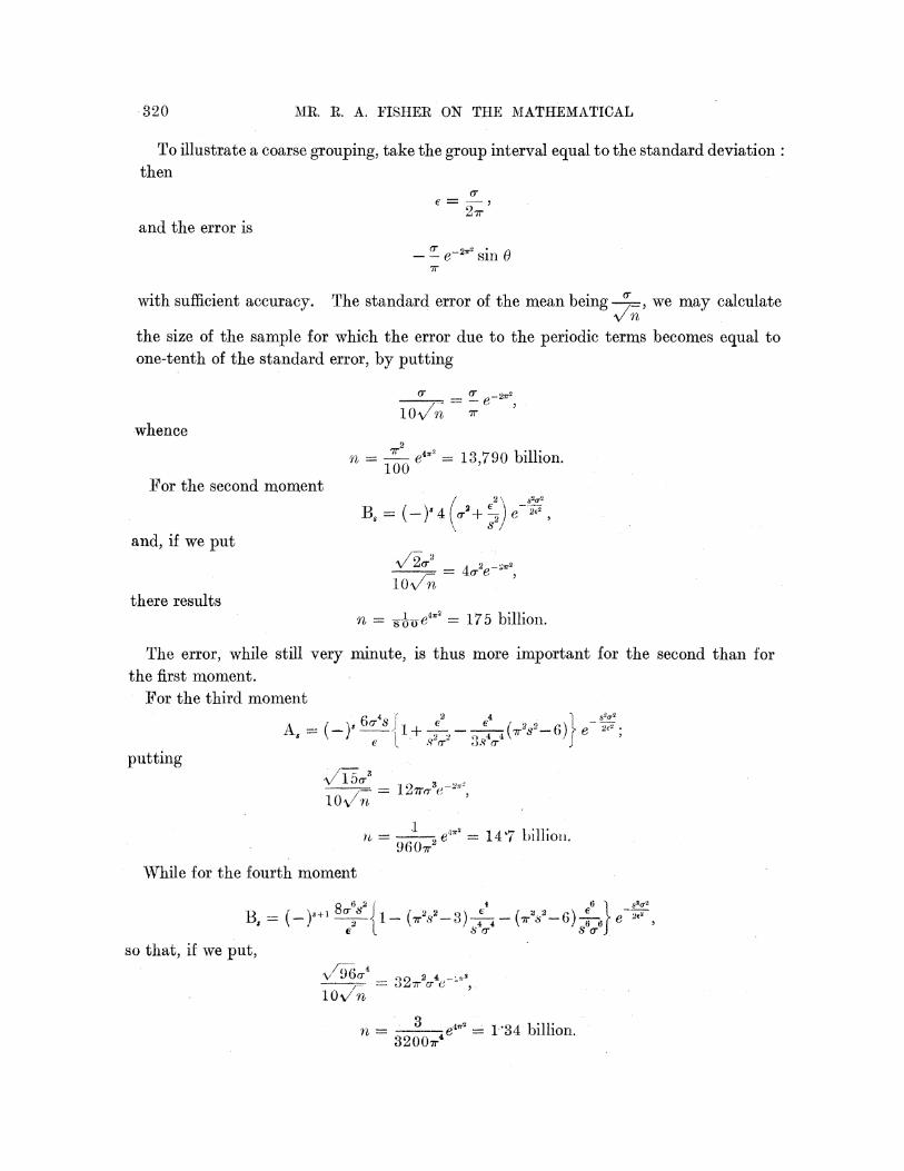
To illustrate a coarse grouping, take the group interval equal to the standard deviation: then

2r e =_

and the error is a' 2,12 - - e- sin 0 7F

with sufficient accuracy. The standard error of the mean being -, we may calculate V/n

the size of the sample for which the error due to the periodic terms becomes equal to one-tenth of the standard error, by putting

C C _ 27r2

10/n n T whence

n = - e42 = 13,790 billion. 100

For the second moment ( s ( / 2 s2V2

B2 = 2

and, if we put v/22 2 _*<M2 - = 4- e ,

o10/n there results

n = -o-e42r = 175 billion.

The error, while still very minute, is thus more important for the second than for the first moment.

For the third moment s 48 2

F4 2 292\ A ~ (Sd e4+

A, = (--)s - I + 6,_ 3 4

S 6s 'e 2

putting

2/10v/n

= 2 e=' = 14 7 billion.

While for the fourth moment

Q 6^ f f 6 1 s30'2

B= (-) -(7r2_3) 4 (7r2-6) e 22

so that, if we put, v/96 . 2- 4.244

n = -- e4 = 1- 34 billion. 32007r4


In a similar manner the exact form of SHEPPARD'S correction may be found for other curves ; for the normal curve we may say that the periodic terms are exceedingly minute so long as a is less than -, though they increase very rapidly if a is increased beyond this point. They are of increasing importance as higher moments are used, not only absolutely, but relatively to the increasing probable errors of the higher moments. The principle upon which the correction is based is merely to find the error when the moments are calculated from an infinite grouped sample; the corrected moment therefore fulfils the criterion of consistency, and so long as the correction is small no greater refinement is required.

Perhaps the most extended use of the criterion of consistency has been developed by PEARSON in the " Method of Moments." In this method, which is without question of

great practical utility, different forms bf frequency curves are fitted by calculating as

many moments of the sample as there are parameters to be evaluated. The parameters chosen are those of an infinite population of the specified type having the same moments as those calculated from the sample.

The system of curves developed by PEARSON has four variable parameters, and may be fitted by means of the first four moments. For this purpose it is necessary to confine attention to curves of which the first four moments are finite; further, if the accuracy of the fourth moment should increase with the size of the sample, that is, if its probable error should not be infinitely great, the first eight moments must be finite. This restriction requires that the class of distribution in which this condition is not fulfilled should be set aside as " leterotypic," and that the fourth moment should become

practically valueless as this class is approached. It should be made clear, however, that there is nothing anomalous about these so-called " heterotypic " distributions

except the fact that the method of moments cannot be applied to them. More- over, for that class of distribution to which the method can be applied, it has not been shown, except in the case of the normal curve, that the best values will be obtained by the method of moments. The method will, in these cases, certainly be serviceable in yielding an approximation, but to discover whether this approximation is a good or a bad one, and to improve it, if necessary, a more adequate criterion is

required. A single example will be sufficient to illustrate the practical difficulty alluded to

above. If a point P lie at known (unit) distance from a straight line AB, and lines be drawn at random through P, then the distribution of the points of intersection with AB will be distributed so that the frequency in any range dx is

= 1 dx df =

7' 1 + (X-m)2

in which x is the distance of the infinitesimal range dx from a fixed point 0 on the line, and m is the distance, from this point, of the foot of the perpendicular PM. The distri-

321

IMR,. R. A. FISHER ON THE MATHEMATICAL

bution will be a svyumetrical one (Type VII.) having its centre at x =-m v (fig. 1). It is therefore a perfectly definite problem to estimate the value of m (to find the best value of m) from a random sample of values of x. We have stated the problem in its simplest possible form: only one parameter is required, the middle point of the distribution.

-6 -5 -4 -3 -2 -10 1 2 3 4 5 6

Fig. 1. Symmetrical error curves of equal intrinsic accuracy.

A . .f . . . . . +

rr l+x2.

B . . . . . . . e 4

By the method of moments, this should be given by the first moment, that is by the mean of the observations: such would seem to be at least a good estimate. It is, however, entirely valueless. The distribution of the mean of such samples is in fact the same, identically, as that of a single observation. In taking the mean of 100 values of x, we are no nearer obtaining the value of m than if we had chosen any value of x out of the 100. The problem, however, is not in the least an impracticable one: clearly from a large sample we ought to be able to estimate the centre of the distribution with some precision; the mean, however, is an entirely useless statistic for the purpose. By taking the median of a large sample, a fair approximation is obtained, for the standard

error of the median of a large sample of n is 2- which, alone, is enough to show that

by adopting adequate statistical methods it must be possible to estimate the value for m, with increasing accuracy, as the size of the sample is increased.

This example serves also to illustrate the practical difficulty which observers often find, that a few extreme observations appear to dominate the value of the mean. In these cases the rejection of extreme values is often advocated, and it may often happen that gross errors are thus rejected. As a statistical measure, however, the rejection of observations is too crude to be defended: and unless there are other reasons for rejection than mere divergence from the majority, it would be more philosophical to accept these extreme values, not as gross errors, but as indications that the distribution of errors is not normal. As we shall show, the only Pearsonian curve for which the mean

322


is the best statistic for locating the curve, is the normal or gaussian curve of errors. If the curve is not of this form the mean is not necessarily, as we have seen, of any value whatever. The determination of the true curves of variation for different types of work is therefore of great practical importance, and this can only be done by different workers recording their data in full without rejections, however they may please to treat the data so recorded. Assuredly an observer need be exposed to no criticism, if after

recording data which are not probably normal in distribution, he prefers to adopt some value other than the arithmetic mean.

6. FORMAL SOLUTION OF PROBLEMS OF ESTIMATION.

The form in which the criterion of sufficiency has been presented is not of direct assistance in the solution of problems of estimation. For it is necessary first to know the statistic concerned and its surface of distribution, with an infinite number of other statistics, before its sufficiency can be tested. For the solution of problems of estimation we require a method which for each particular problem will lead us

automatically to the statistic by which the criterion of sufficiency is satisfied. Such a method is, I believe, provided by the Method of Maximum Likelihood, although I am not satisfied as to the mathematical rigour of any proof which I can put forward to that effect. Readers of the ensuing pages are invited to form their own opinion as to the possibility of the method of the maximum likelihood leading in any case to an insufficient statistic. For my own part I should gladly have withheld publication until a rigorously complete proof could have been formulated; but the number and variety of the new results which the method discloses press for publication, and at the same time I am not insensible of the advantage which accrues to Applied Mathematics from the co-operation of the Pure Mathematician, and this co-operation is not infrequently called forth by the very imperfections of writers on Applied Mathematics.

If in any distribution involving unknown parameters 0,, 02, 0,..., the chance of an observation falling in the range dx be represented by

f(x, 0, 02, ... ) dx,

then the chance that in a sample of n, n, fall in the range dx,, n2 in the range dx2, and so on, vwill be

( (!) f ( v, 01, 02, ... ) dx)'n

The method of maximum likelihood consists simply in choosing that set of values for the parameters which makes this quantity a maximum, and since in this expression the parameters are only involved in the functionf, we have to make

S (logf)

323


a maximum for variations of 01, 02, 0, &c. In this form the method is applicable to the fitting of populations involving any number of variates, and equally to discontinuous as to continuous distributions.

In order to make clear the (listinction between this Imethod and that of BAYES, we

will apply it to the same type of probleim as that wvhich BAYES discussed, in the hope of making clear exactly of wThat kind is the information which a sample is capable of

supplying. This question naturally first arose, not with respect to populations distributed in frequency curves and surfaces, but with respect to a population regarded as divided into two classes only, in fact in problems of probability. A certain proportion, p, of an infinite population is supposed to be of a certain kind, e.g., " successes," the remainder are then " failures." A sample of n is taken and found to contain x successes and y failures. The chance of obtaining such a sample is evidently

! P'(1-P)Y

Applying the method of maximum likelihood, we have

S (logf) = x log p+y log (I -)

whence, differentiating with respect to p, in order to make this quantity a maximum,

y A x --= _ , or - -. p 1p n

The question then arises as to the accuracy of this determination. This question was first discussed by BAYES (10), in a form which we may state thus. After observing this sample, when we know p, what is the probability that p lies in any range dp ? In other words, what is the frequency distribution of the values of p in populations which are selected by the restriction that a sample of n taken from each of them yields x successes. Without further data, as BAYES perceived, this problem is insoluble. To render it capable of mathematical treatment, BAYES introduced the datum, that among the populations upon which the experiment was tried, those in which p lay in the range dp were equally frequent for all equal ranges dp. The probability that the value of p lay in any range dp was therefore assumed to be simply dp, before the sample was taken. After the selection effected by observing the sample, the probability is clearly proportional to

px ( l-p)Ydp.

After giving this solution, based upon the particular datum stated, BAYES adds a scholium the purport of which would seem to be that in the absence of all knowledge save that supplied by the sample, it is reasonable to assume this particular a priori distribution of p. The result, the datum, and the postulate implied by the scholium, have all been somewhat loosely spoken of as BAYES' Theorem.

324


The postulate would, if true, be of great importance in bringing an immense variety of questions within the domain of probability. It is, however, evidently extremely arbitrary. Apart from evolving a vitally important piece of knowledge, that of the exact form of the distribution of values of p, out of an assumption of complete ignorance, it is not even a unique solution. For we might never have happened to direct our attention to the particular quantity p: we might equally have measured probability upon an

entirely different scale. If, for instance,

sin 0 = 2p -1,

the quantity, 0, measures the degree of probability, just as well as p, and is even, for some purposes, the more suitable variable. The chance of obtaining a sample of x successes and y failures is now

! (1 +sin 0) ( 1-sin 0)Y; 2 x y!

applying the method of maximum likelihood,

S (logf) = x log (1 +siin 0) +y log ( -sin 0) -n log 2,

and differentiating with respect to 0,

x cos 0 y cos 0 . y xcos0 _ ycos0 whence sin 0 - l.+sn 0 1-sinO' 2n

an exactly equivalent solution to that obtained using the variable p. But what a priori assumption are we to make as to the distribution of 0 ? Are we to assume that 0 is

equally likely to lie in all equal ranges do ? In this case the a priori probability will be d0/7r, and that after making the observations will be proportional to

(1 + sin 0)x ( -sin o0) d0.

But if we interpret this in terms of p, we obtain

px (1-P)y dp p- (1 -p)Y dp, vp (1-p)"

a result inconsistent with that obtained previously. In fact, the distribution previously assumed for p was equivalent to assuming the special distribution for 0,

cos 0 df= de,

the arbitrariness of which is fully apparent when we use any variable other than p. In a less obtrusive form the same species of arbitrary assumption underlies the method VOL. CCXXII.-A, 2 4

325


known as that of inverse probability. Thus, if the same observed result A might be the consequence of one or other of two hypothetical conditions X and Y, it is assumed that the probabilities of X and Y are in the same ratio as the probabilities of A occurring on the two assumptions, X is true, Y is true. This amounts to assuming that before A was observed, it was known that our universe had been selected at random for an infinite population in which X was true in one half, and Y true in the other half. Clearly such an assumption is entirely arbitrary, nor has any method been put forward by which such assumptions can be made even with consistent uniqueness. There is nothing to prevent an irrelevant distinction being drawn among the hypothetical conditions represented by X, so that we have to consider two hypothetical possibilities X, and X2, on both of which A will occur with equal frequency. Such a distinction should make no difference whatever to our conclusions; but on the principle of inverse probability it does so, for if previously the relative probabilities were reckoned to be in the ratio x to y, they must now be reckoned 2x to y. Nor has any criterion been suggested by which it is possible to separate such irrelevant distinctions from those which are relevant.

There would be no need to emphasise the baseless character of the assumptions made under the titles of inverse probability and BAYES' Theorem in view of the decisive criticism to which they have been exposed at the hands of BOOLE, VENN, and CHRYSTAL, were it not for the fact that the older writers, such as LAPLACE and POISSON, who accepted these assumptions, also laid the foundations of the modern theory of statistics, and have introduced into their discussions of this subject ideas of a similar character. I must indeed plead guilty in my original statement of the Method of the Maximum Likeli- ]lood (9) to having based my argument upon the principle of inverse probability; in the same paper, it is true, I emphasised the fact that such inverse probabilities were relative only. That is to say, that while we might speak of one value of p as having an inverse probability three times that of another value of p, we might on no account introduce the differential element dp, so as to be able to say that it was three times as probable that p should lie in one rather than the other of two equal elements. Upon consideration, therefore, I perceive that the word probability is wrongly used in such a connection: probability is a ratio of frequencies, and about the frequencies of such values we can know nothing whatever. We must return to the actual fact that one value of p, of the frequency of which we know nothing, would yield the observed result three times as frequently as would another value of p. If we need a word to characterise this relative property of different values of p, I suggest that we may speak without confusion of the likelihood of one value of p being thrice the likelihood of another, bearing always in mind that likelihood is not here used loosely as a synonym of probability, but simply to express the relative frequencies with which such values of the hypothetical quantity p would in fact yield the observed sample.

The solution of the problems of calculating from a sample the parameters of the hypothetical population, which we have put forward in the method of maximum likeli-

326


hood, consists, then, simply of choosing such values of these parameters as have the maximum likelihood. Formally, therefore, it resembles the calculation of the mode of an inverse frequency distribution. This resemblance is quite superficial: if the scale of measurement of the hypothetical quantity be altered, the mode must change its position, and can be brought to have any value, by an appropriate change of scale; but the optimum, as the position of maximum likelihood may be called, is entirely unchanged by any such transformation. Likelihood also differs from probability* in that it is not a differential element, and is incapable of being integrated : it is assigned to a particular point of the range of variation, not to a particular element of it. There is therefore an absolute measure of probability in that the unit is chosen so as to make all the elementary probabilities add up to unity. There is no such absolute measure of likelihood. It may be convenient to assign the value unity to the maximum value, and to neasure other likelihoods by comparison, but there will then be an infinite number of values whose likelihood is greater than one-half. The sum of the likelihoods of admissible values will always be infinite.

Our interpretation of BAYES' problem, then, is that the likelihood of any value of p is proportional to

pX (1p)Y,

and is therefore a maximum when x . . . . p --- _,-7 n

which is the best value obtainable from the sample; we shall term this the optimum value of p. Other values of p for which the likelihood is not much less cannot, however, be deemed unlikely values for the true value of p. We do not, and cannot, know, from the information supplied by a sample, anything about the probability that p should lie between any named values.

The reliance to be placed on such a result must depend upon the frequency distribution of x, in different samples from the same population. This is a perfectly objective statistical problem, of the kind we have called problems of distribution ; it is, however, capable of an approximate solution, directly from the mathematical form of the likelihood.

When for large samples the distribution of any statistic, 01, tends to normality, we

* It should be remarked that likelihood, as above defined, is not only fundamentally distinct from mathematical probability, but also from the logical " probability " by which Mr. KEYNES (21) has recently attempted to develop a method of treatment of uncertain inference, applicable to those cases where we lack the statistical information necessary for the application of mathematical probability. Although, in an important class of cases, the likelihood may be held to measure the degree of our rational belief in a conclusion, in the same sense as Mr. KEYNES' " probability," yet since the latter quantity is constrained, somewhat arbitrarily, to obey the addition theorem of mathematical probability, the likelihood is a

quantity which falls definitely outside its scope. 2 z 2

327

MR . A. A FISHER ON THE MATHEMATICAL

may write down the chance for a given value of the parameter 0, that 0, should lie in the range do, in the form

( 01 (-0)

$ ==-=:e d6,.

The mean value of 0, will be the true value 0, and the standard deviation is a-, the

sample being assumed sufficiently large for us to disregard the dependence of aC upon O. The likelihood of any value, 0, is proportional to

(e, -ey2

this quantity having its maximum value, unity, when

log 0;

Differentiating now a second time

2" 1 a02 log : 2= 2

Now 4) stands for the total frequency of all samples for which the chosen statistic has the value 01, consequently =- S' (0), the summation being taken over all such examples, where /s stands for the probability of occurrence of a certain specified sample. For which we know that

iog p = CJ+S (logf), the summation being taken over the individual members of the sample.

If now we expand logf in the form

--2

log f (0) logf (0) ?-, log (0) + log f(o,) f ...,)

or

log f = log i + 0-01+ 2 0-0 +..., we have

log = c+0-0os(a)+0-01e, (b)+...; now for optimum statistics

S (a) 0,

and for sufficiently large samples S (b) differs from nb only by a quantity of order v/nab ; moreover, 0-01 being of order n-~, the only terms in log p which are not reduced without limit, as n is increased, are

log C + nT_0 ;

328


hence

^oc e~ ?----.

Now this factor is constant for all samples which have the same value of 0,, hence the variation of 4) with respect to 0 is represented by the same factor, and conse-

quently log q = C'+nn b 0-01;

whence 1 a2

2--; = ~-flog I = n6,

where

b -= logf(01), p32

01 being the optimum value of 0. The formula

- = ax log

supplies the most direct way known to me of finding the probable errors of statistics. It may be seen that the above proof applies only to statistics obtained by the method of maximum likelihood.*

For example, to find the standard deviation of

A X

n

* A similar method of obtaining the standard deviations and correlations of statistics derived from

large samples was developed by PEARSON and FILON in 1898 (16). It is unfortunate that in this memoir no sufficient distinction is drawn between the population and the sample, in consequence of which the formulae obtained indicate that the likelihood is always a maximum (for continuous distributions) when the mean of each variate in the sample is equated to the corresponding mean in the population (16, p. 232,

A, = 0 "). If this were so the mean would always be a sufficient statistic for location; but as we have already seen, and will see later in more detail, this is far from being the case. The same argument, indeed, is applied to all statistics, as to which nothing but their consistency can be truly affirmed.

The probable errors obtained in this way are those appropriate to the method of maximum likelihood, but not in other cases to statistics obtained by the method of moments, by which method the examples given were fitted. In the ' Tables for Statisticians and Biometricians ' (1914), the probable errors of the constants of the Pearsonian curves are those proper to the method of moments; no mention is there made of this change of practice, nor is the publication of 1898 referred to.

It would appear that shortly before 1898 the process which leads to the correct value, of the probable errors of optimnum statistics, was hit upon and found to agree with the probable errors of statistics found

by the method of moments for normal curves and surfaces; without further enquiry it would appear to have been assumed that this process was valid in all cases, its directness and simplicity being peculiarly attractive. The mistake was at that time, perhaps, a natural one; but that it should have been discovered and corrected without revealing the inefficiency of the method of moments is a very remarkable circumstance.

In 1903 the correct formulhe for the probable errors of statistics found by the method of moments are

given in ' Biometrika ' (19); references are there given to SHEPPARD (20), whose method is employed, as well as to PEARSON and FILON (16), although both the method and the results differ from those of the latter.

329


in samples from an infinite population of which the true value is p,

logf = log p+ y log ( -p),

l * .' x y

_x y -log f = --- ap2 p lI-p

Now the mean value of x in pn, and of y is (l--p) n, hence the mean value of

-logfi 1 is-

therefore 2_p(L-p)

2'~ - --

n

the well-known formula for the standard error of p.

7. SATISFACTION OF THE CRITERION OF SUFFICIENCY.

That the criterion of sufficiency is generally satisfied by the solution obtained by the method of maximum likelihood appears from the following considerations.

If the individual values of any sample of data are regarded as co-ordinates in

hyperspace, then any sample may be represented by a single point, and the frequency distribution of an infinite number of random samples is represented by a density distribution in hyperspace. If any set of statistics be chosen to be calculated from the samples, certain regions will provide identical sets of statistics; these may be called isostatistical regions. For any particular space element, corresponding to an actual

sample, there will be a particular set of parameters for which the frequency in that element is a maximum; this will be the optimum set of parameters for that element. If now the set of statistics chosen are those which give the optimum values of the

parameters, then all the elements of any part of the same isostatistical region will contain the greatest possible frequency for the same set of values of the parameters, and therefore any region which lies wholly within an isostatistical region will contain its maximum frequency for that set of values.

Now let 0 be the value of any parameter, 0 the statistic calculated by the method of maximum. likelihood, and 01 any other statistic designed to estimate the value of 0, then for a sample of given size, we may take

f (, 0, e1)d do1d

to represent the frequency with which 0 and 0, lie in the assigned ranges do and dol.

330


The region dOdol evidently lies wholly in the isostatistical region d4. Hence the equation

a log/f(, 4, 1) = o

is satisfied, irrespective of 01, by the value 0 = . This condition is satisfied if

y(0, 0, o ,)= ) (o, 4) 0'.0 (, 0); for then

alog =a log ,

and the equation for the optimum degenerates into

i log q (, 4) 0,

which does not involve 01. But the factorisation of f into factors involving (0, 6) and (4, 01) respectively is merely

a -mathematical expression of the condition of sufficiency; and it appears that any statistic which fulfils the condition of sufficiency must be a solution obtained by the method of the optimum.

It may be expected, therefore, that we shall be led to a sufficient solution of problems of estimation in general by the following procedure. Write down the formula for the probability of an observation falling in the range dx in the form

f(0, x) dx,

where 0 is an unknown parameter. Then if

L= S(logf)

the summation being extended over the observed sample, L differs by a constant only from the logarithm of the likelihood of any value of 0. The most likely value, 0, is found by the equation

aL -= O, 80

and the standard deviation of 4, by a second differentiation, from the formula

2_L 1,

802 ~ 2

this latter formula being applicable only where 6 is normally distributed, as is often the case with considerable accuracy in large samples. The value 0- so found is in these cases the least possible value for the standard deviation of a statistic designed to

331

MR. R. A. FISHER: ON THE MATHEMATICAL

estimate the same parameter; it may therefore be applied to calcullate the efficiency of

any other such statistic. When several parameters are determnined simultaneously, we nmust equate the second

differentials of L, with respect to the parameters, to the coefficients of the quadratic terms in the index of the normal expression which represents the distribution of the

corresponding statistics. Thus with two parameters,

a2L 1 1 a1 L I1

a2L 1 r

-2 - - 2.-r 2. a - 2. 4'

2J __ 1 r a01 ae3 1O _ r -r2* a2 a

or, in effect, a(r is found by dividing the Hessian determinant of L, with respect to the

parameters, into the corresponding minor. The application of these methods to such a series of parameters as occur in the speci-

fication of frequency curves may best be made clear by an example.

8. THE EFFICIENCY OF THE METHOD OF MOMENTS IN FITTING CURVES OF THE

PEARSONIAN TYPE III.

Curves of PEARSON's Type III. offer a good example for the calculation of the efficiency of the Method of Moments. The chance of an observation falling in the range dx is

drV= -. -6 e a dx.*

By the method of moments the curve is located by means of the statistic u, its dimen- sions are ascertained from the second moment ,2, and the remaining parameter p is determined from ,3. Considering first the problem of location, if a and p were known and we had only to determine m, we should take, according to the method of moments,

- A= m,+ (p+ 1),

where m~ represents the estimate of the parameter m, obtained by using the method of moments. The variance of m, is, therefore,

2 2 = , 2a +1)

If, on the other hand, we aim at greater accuracy, and make the likelihood of the sample a maximum for variations of In, we have

L =-n log a-n log (p !) +pS ( log xm ) -S(),

* The expression, x !, is used here and throughout as equivalent to the Gaussian II (x), or to r (+l 1), whether x is an integer or not.

332

FOUNDATIONS O THE' REE()'TICAr- SrTATrISTICS,. 833

and the equation to determine m is

L., -p 1S ('A = -PS - +- . ; . . .

(1) Cm \x-m/ a *

the accuracy of the value so obtained is found fromr the second differential,

,m2 ':\'-p/ of which the mean value is

whence

( - - n

We now see that the efficiency of location by the method of lmomlents is

2p-) I- 1. P +1 p + 1

Efficiencies of over 80 per cent. for location are therefore obtained if p exceeds 9; for

p = 1 the efficiency of location vanishes, as in other cases where the curve makes an

angle with the axis at the end of its range. Turning now to the problem of scaling, we have, by the method of moments,

.2 =, (2 + l ),

whence, knowing p, a is obtained. Since

2 2 [-1 2

we must have 2 p321 2 4 + 3

, 2 ___ 2 2

c-r 4n 8n 2 (p+t) ,

on the other hand, from the value of L, we find the equation

|L^ k n(p+ l)+iS(^-) , (2)

to be solved for m and a as a simultaneous equation with (1) ; whence

Ia_, am a a- t

and a2L (p.) s(-.) ;' Ca a5

3 -\ VOL(. CoXXInl. -- A.

334 MAf. RA.A, FISHER ON THIE MATHEMATICAIL

of which !thie jmean vaflue is n(p 1.)

a2

dividing

cr c (p-1) by the dete rminant

~" (){p .) , 9t,a

__ n_ a _ (p + ) (2

which reduces to 2 ^

whence a .....

2/,

and the efficiency of sca,lng )by the method of moments is

p?l 3

p+ 4 p+ 4

Efficiency of over 80 per cent. for scaling are, therefore, obtained when p exceeds 11.

The efficiency of scaling does not, however, vanish for any possible value of p, though it tends to zero, as p approaches its limiting value, -1.

Lastly, p is found by the method of m:oments by putting

4

p + 1 Now

- _ /2 ('434-242 + 36 + 90/3-12'33 51),

and for c:rves of r'ypel 11II,

/,2 3 + V

/ - (s + 23, 3) = -a/ (3A+.:S + 6), hence

2 = ...t.(5Afi + 4) (/, + 4),

_ 63 ((p+ 2) (p, +6) 1 , ' p+

FOUNDATIONS OF THEORETICAL STATISTICS, 335

whence it follows, since n is large, that

2 = 6(+. L | + ( 1)(p+)2) (p +6). * = " .. np+ -

From the value of L,

L d '-. = --n - log (p!) + S log --- ,

which equation solved for m, a and p as a simultaneous equation with (1) and (2), w-il yield the set of values for the parameters which has the maximum likelihood. To find the variance of the value of p, so obtained, observe that

c?m p \xI /I

of which the mean value is . - ,~~~~~~a

BaL p - _ aa ap - 2'

a2L = 3

f (I , p

- 2 ,log !).

and

The variance of p, derived from this set of simultaneous equations, is tlherefore found

by dividing the minor of a L namely *

3p -

2 n2

P- ]e adt by the determinant

(t4 p-1

1

1

P .

hence

When p is large,

. 1 P

p+1 1 d2 -- log

-(1p 12

~~(p}v~!)l (

ct p - dp^ tp-(p

(?')~~~~~

I 2

d' r2d 's2 (+~= .2- log (p!) 2+

(-I 2

in p p 2'

)

2

2. p, 3 2+1},

I"j - .5 ' 7p7 '"'

3 A 2

MR. R. A. FISHEIER ON THE MATHEMATICAL

so that, approximately, 2= 6(p3+'p);

for large values of p, the efficiency of the method of moments is, therefore, approximately

p+ p + 2 p + 6

Efficiencies of over 80 per cent. occur whein p exceeds 381 (,fi -- 0 102); evidently the method of moments is effective for determining the form of the curve only when it is relatively close to the normal form. For small values of p, the above approximation for the efficiency is not adequate. The true values can easily be obtained from the recently published tables of the Trigarima* function (ll). The following values are obtained for the integral values of p from 0 to 5.

p 0 1 2 3 4 5

Efficiency . . . 0 0-0274 0-0871 0-1532 0-2159 0-2727

An interesting point which may be resolved at this stage of the enqulir is to find the variance of m, when a and p are not known, derived from the above set of simultaneous equations; that is to say, to calculate the accuracy with which the limiting point of the curve is determined; such determinations are often stated as the result of fitting curves of limited range, but their probable errors are seldonl, if ever, evaluated. To obtain the greatest possible accuracy with which such a point can be determined

we must divide the minor of ,, namely,

{p+1- log(p!)d2 i by

n3 _L_ __ 1 - * \2 log (p !) + , (t4 p-g (dp2 lVP'I /

p2p" whence

2 (tp 1 p + dpS log (!)- 1 d 2d" 2 1 2 log (p!)- + 2

dp2 p p

The position of the limiting point will, when p is at all large, evidently be determined with mtuch less accuracy than is the position, as a whole, of a curve of known form and size. Let n' be a multiplier such that the position of the extremity of a curve calculated

d2 * It is sometimes convenient to write (x) for - log (x). fo vlo (!)

3 %f6

FiOUNI )AIONS OF THrEOlRETICATL STAT.ISTICS.

from nn' observations will be determined with the same accuracy as the position, as a

whole, of a curve of known form and size, can be determined from a sample of n observations when n is large. Then

P 4 2 log (p!) -1.

2--- log (p!)-- ? ..- Up22 + P' but, when p is large,

d2 2 p?1 log (p!) -t . .....-.l-() .P + log (P - - + 2 ... ;p ~ ~ '\3p 3p/

and d2 2 22 log (p i) + = 3 );

therefore

el/ 2

p3(_2 p 8 ) 3 3 p + -

"

- = 3Jp-p+2

For large values of p the probable error of the determiination of the end-point may be found approximately by multiplying the probable error of location by

(p-?) -3/-.

As p grows smaller, n' diminishes until it reaches unity, when p-- 1. For values of

p less than 1 it would appear that the end-point had a smaller probable error than tle probable error of location, but, as a matter of fact, for these values location is determined

by the end-point, and as we see from the vanishing of o^, whether or not p and a are known, when p - 1, the weight of the determination from this point onwards increases more rapidly than n, as the sample increases. (See Section 10.)

The above method illustrates how it is possible to calculate the variance of any function of the population. pa rameters as estimated from large samples by comparirng this variance with th that of the sae function estimated by the methiod of mloments, we

may find the efficiency of that method for any proposed function. Thle above examnina-

tion, in which the determinations of the locus, the scale, and the forim of the curve are

treated separately, will serve as a general criterion of the application of the method of moments to curves of Type III. Special combinations of the parameters will, however, be of interest in special cases. It may be noted here that by virtue of equation (2) the function of rm -1-- a (p - I) is the same, whether determined by moments or by the method of the optimum :

, + Ca (p-L+ 1) = n + ? ( + 1).

The efficiency of the method of moments in deter this function is therefore 100

per cent. 'rhat this function is the abscissa of the mean does not imply 100 per cent.

efficiency of location, for the centre of location of these curves is not the mean (see p. 340).

337

1MR. R. A. FISHER ON THE MATHEM[ATICALT

9. LOCATION AND SCALING OF FREQUENCY CURVES IN GENERAL.

The general problem of the location and scaling of curves may now be treated more generally. This is the problem which presents itself with respect to error curves of assumed form, when to find the best value of the quantity mleasured we must locate the curve as accurately as possible, and to find the probable error of the result of this process we must, as accurately as possible, estimate its scale.

The form of the curve may be specified by a fun ction (,, s-uch that

3;, --'D 1 d j' c c~ ) de, when e = -.

In this expression < specifies the form of the curve, which is unaltered by variations of a an(I m.

When a sample of n observations has been taken, the likelihood of any combination of values of a and m is

L -( C- lfog aC+S (I), whence

aL = am (dl dAm a

since

a8 a also

?L 1: Q /- ,, 8a t (at

since at _ t. aa a

Differentiating a second time, a2L 1 , -- -- -b _(p ) ,

therefore

(rhi -e 't,a

This expression enables us to compare the accuracy of error curves of different form, when the location is performed in each case by the method which yields the minimum error.

Example -The curve d

d(/' - 7r 1 +- ?

referred to in Section 5 has an infinite standard deviation, but it is not on that accolunt an error curve of zero accuracy, for

,-log ( +)," = _ +2 )2 I~~/ - (1? ii$ ')2

338

FOUNI)ATIONS OFt' THEO)RETICAI, STATISTlICS 339

Now

hence --i. ct < CT; (f" = -} and c-~ = ?

The quantity, X 81 a2 2a2t

which is the factor by which n is multiplied in calculatiing the weight of the estimate made from rn mleasurements, may be called the intrinsic accuracy of an error curve. In the above example we see that errors distributed so that

d a d ,2 X2

have the samle intrinsic accuracy as errors distributed according to the normal curve

df -- 2-e2x (Ix

provided 2 ) 2

Fig. 1 illustrates two such curves of equal intrinsic accuracy. Returning now to the general problem. in which

L J= C- log +S (), we have

c L s (+ ) s (fF) C(:1 a ct a 0,

and

a:L = 8 (2 '+r ?" ) '

C =1 S (+"- ).

The latter expression will. directly give the accuracy witi which a is determined only if

m c -c-0 Qm da

and we can always arrange thiat this shall be so by subtracting from E the quantity

")!

Thus in a Type III. curve where, referred to the end of the range,

9-1 1, b,v =--1, (/)" = - 1

340 MIR. . A. FISITER ON THIlE MATHEMATICAL

instead of ,p = p log c-$

we must write

j = log t+P- - +~ - 1; then

_,+ p-/l '

?f+p_ hence

_2L = (120_1

'' ( ' $+P-1 +p-1_

of which the mean value is

(- +2p- -p-: --) = -

,

hence 22

2n

2n

For one particular point of origin, therefore, the variations of the abscissa are uincorrelated with those of a; this point may be termed the centre of location.

Example :--To determine the centre of location of the curve of Type IV.,

df e-v tall- (L + :- r + ?2

Here

=-v tan-l r + 2

log T g,

-2 9' = - (v+,+ 2 ) I +t~ ,

g" = r+ + 2 2 +2 (v--r +2) 1 + 2;

from these we find

i'+4 +?r2 r++ 1 ,r+2 r+ (f

=- -2 2

qr+4 +ir

r}+ 4 +IJ

so that

e4 ?

The centre of location, therefore, at the distance fro+ the mode,

rvt- ) "~+4'

FOUNDATIONS OF THEORETICAL STATISTICS. 341

:Exmnple :-Determine the intrinsic acculracy of an error curve of Type IV. and tle

efficiency of the method of moments in location and scaling.- Since

777 _ 1 r r+2r +4 r-+4 +v2

2 ~2 v2 2 a r+4 +v

8rh + l r +- 2 r -- 4 n ,-+lr+2r+4

and the intrinsic accuracy of the curve is

1 r+1r+2 i2r+4 a ----_- 2

a r+4 +v2 but

2 -a(2 .a2+ v2 ~ n --r2

therefore the efficiency of tte method of moments in location is

- 1 (r+ 2 +2) ^r27^ 24-^ V(3)

r-+l ,+2r+4(r24-2) a( /

When v= 0, we have for curves of Type VII. an efficiency of location

6 ,1 + 1 r +2

The efficiency of location of these curves vanishes at r = 1, at which value the standard deviation becomes infinite. Although values down to --1 give admissible frequency curves, the conventional limit at which curves are reckoned as heterotypic is at r = 7. For this value the efficiency is

49 121+ v 132 49+v2 '

which varies from 91*'67 per cent. for the symmetrical Type VII. curve, to 37*12 per cent. when v ->- o and the curve to Type V.

Turning to the question of scaling, we find

~f~"- 1 = ?( r-+2r +4+v) 2 2

r+4 +v2 whence

(- = r+4 anld

2 a2 a r+4 ct - -- : 2

'

n 2r+l 3 B VOL. CCXXII.-A.


the intrinsic accuracy of scaling is therefore independent of i,. Now for thlese curves

3r--1 8'? 2

2 = 2 ' 3 - +6 - 2 4'1 r-2r-3\ r+v/2

so that /32-1 _r3 r-2 + 2 (r2+ 10r-12)

4 r-2 r-3 (r2+2) and

2 a2 r3 -2 + 2 lv(r2+10r-12) a, n'- 2 r- 3 (r2 + 2)

The efficiency of the method of moments for scaling is thus

r-2 r-3 r+4 (+ v2 ) (4 r+1 {ri3r--+2 v2(.2+l Or-12)}'

when v- =O, we have for curves of Type VII. an efficiency of scaling

L2

1r +1

The efficiency of the miethod of mnomlents iii scaling these curves vanishes at r - 3, where ,2 becomes infinite; for r - 7, the efficiency of scaling is

55 49+v 2 ' 1715+107v:'

varying in value from 78-57 per cent. for the symmetrical Type VII. curve, to 25*70

per cent. when v -> oo and the curve to Type V.

10. THE EFFICIENCY OF THE METHOD OF MOMENTS IN FITTING THE PEARSONIAN

CURVES.

The Pearsonian group of skew curves are obtained as solutions of the equation

1 dy _ -(x-r) .

y dx a + bx + cx2 '

algebraically these fall into two main classes,

df (i+2 ( li-) dx

and

( -" X) 2e -vtanlr df 2: e a dx,

a/

according as the roots of the quadratic expression in (5) are real or imaginary.


The first of these forms may be rewritten

?i(i a2 r+2

dfj 1-2 ) a dx,

r being negative, showing its affinity with the second class. In order that thlese expressions may represent frequency curves, it is necessary that

the integral over the whole range of the curve should be finite; this restriction acts in two ways:-

(1) When the curve terminates at a finite value of x, say x = a., the power to which

a2--x is raised must be greater than - 1.

(2) When the curve extends to infinity, the ordinate, when x is large, must diminish

more rapidly than -; x

Tn Fig. 2 is shown a conspectus of all possible frequency curves of the Pearsonian type; A

A.

_.. Y= O0

. . . .... HeHerotypic Limit r 7

. ..- .- .--. LimitoF( diagram r3

C

B. Showing region of validity of second moment.

Fig. 2. Conspectus of Pearsonian system of frequency curves. 3 :B 2

343


the lines AC and AC' represent the limits along which the area between the curve and a vertical ordinate tends to infinity, and on which il,, or mn,, takes the value -- 1 ; the line CC' represents bhe limit at which unbounded curves enclose an i:nfinite area with the horizontal axis; at this limit r - -1.

The symmetrical curves of Type II.

2' \ r4~-2 d I z (~t -)

?

extend from the point N, representing the normal curve, at which r is infinite, through the point P at which r --4, and the curve is a parabola, to the point B (r - -2), where the curve takes the form of a rectangle ; from this point the curves are U-shaped, and at A, when the arms of U are hyperbolic, we have the limiting curve of this type, which is the discontinuous distribution of equal or unequal dichotomy ('r - 0).

Tr-le unsymmetrical curves of Type I. are divided by PEARSON into three classes

according as the terminal ordinate is infinite at neither end, at one end (J curves)j or at both ends (U curves); the dividing lines are C'BD and CBD', along which one of the terminal ordinates are finite (mn,, or , -- 0) ; at the point B, as we have seen, both terminal ordinates are finite.

The same line of division divides the curves of Type III.,

dcf oc xPe- dx,

at the point E (p = 0), representing a simple exponential curve ; the J curves of Type II I. extend to F (p -1), at which point the integral ceases to converge. In curves of

Type III., r is infinite ; v is also infinite, but one of the quantities mi, and mn2 is finite, or zero (= p); as p tends to infinity we approach the normal curve

df c e-"2 dx.

Type VI., like Type III., consists of curves bounded only at one end; here r is

positive, and both mn and in, are finite or zero. For the J curves of Type VI. both in, and mn, are negative, but for the remainder of these curves they are of opposite sign, the negative index being the greater by at least unity in order that the representative point may fall above CC' (r -1).

Type V. is here represented by a parabola separating the regions of Types IV. and VI.; the typical equation of this type of curve is

- , t .3 1

dYf oc x2 e d x.

As r tends to infinity the curve tends to the normal form; the integral does not

become divergent until ~rk 1, or r -1. On curves of Type V., then, r is finite

or zero, but , is infinite.

344


In Type IV.

-7 f c1 + a^Y1'?" vxtan-1T

cr-l1^2 eI a;

we have written v, not as previously for the difference between ml and m, for these quantities are now complex, and their difference is a pure imaginary, but for the difference divided by /--1; , is then real and finite throughout Type IV., and it vanishes

along the line NS, representing the symmetrical curves of Type VII.

2 9\+2

dfo1+( 2) 2

from r = to or = -1.. The Pearsonian system of frequency curves has hitherto been represented by the

diagram (13, p. 66), in which the co-ordinates are /3 and 2,. This is an unsymmetrical diagram which, since /3l is necessarily positive, places the symmetrical curves on a

boundary, whereas they are the central types from which the unsymmetrical curves diverge on either hand; further, neither of the limiting conditions of these curves can be shown on the /3 diagram; the limit of the U curves is left obscure,* and the other limits are either projected to infinity, or, what is still more troublesome, the line at

infinity cuts across the diagram, as occurs along the line r 3, for there /, becomes infinite. This diagram thus excludes all curves of Types VII., IV., V., and VI., for which

< 3. In the a3 diagram the condition r = constant yields a system of concurrent straight

lines. The basis of the representation in fig. 2 lies in making these lines parallel and

horizontal, so that the ordinate is a function of r only. We have chosen r == y-- -, y

and have represented the limiting types by the simplest geometrical forms, straight lines and parabolas, by taking

4 e 9 92^ +

v2 (

+ _x +-2 2). y (Xz2_y)

It might have been thought that use could have been made of the criterion,

Ai (02+3)2 I-- 4 (482-3/31)(2/2-3A,-6) ( 4?

by which PEARSON distinguishes these curves; but this criterion is only valid in the

region treated by PEARSON. For when r = 0, K2 = 1, and we should have to place a variety of curves of Types VII., TV., V., and VI., all in Type V. in order to adhere to the criterion.

This diagram gives, I believe, the simplest possible conspectus of the whole of the Pearsonian system of curves; the inclusion of the curves beyond r = 3 becomes neces-

* The true limit is the line 2 = PI + 1, along which the curves degenerate into simiple dichotomies.

345.

MR. ER. A. FISHER ON THE MATHEMATICAL

sary as soon as we take a view unrestricted by the method of moments ; of the so-called

heterotypic curves between r = 3 and r = 7 it should be noticed that they not

only fall into the ordinary Pearsonian types, but have finite values for the nmoment coefficients /3, and 32; they differ from those in which r exceeds 7, merely in the fact

that the value of f32, calculated from the fotrth moment of a sample, has an infinite probable error. It is therefore evident that this is not the right method to treat the sample, but this does not constitute, as it has been called, " the failure of Type IV.," b-ut merely the failure of the method of moments to make a valid estimate of the form of these

curves. As we shall see in more detail, the method of moments, when its efficiency is tested, fails equally in other parts of the (diaoram.

In expression (3) we have found that the efficiency of the method of nmoments for location of a curve of Type IV. is

_--2 E=

2 r-"--L (r?+4 v2)

_1 r2t2r+4 (r_ 2)

whence if we substitute for r and , in terms of the co-ordinates of our diagram, we obtain a general formula for the efficiency of t:he method of moments in locating Pearsonian

curves, which is applicable within the boundary of the zero contour (fig. 3). lThis may

0 D

Fig. 3. Region of validity of the first moment (the mean) applied in the location of

Pearsonian curves showing contours of efficiency.

be called the region of validity of the first moiment; it is bounded at the base by the

line r - 1, so that the first monient is valid far beyond the heterotvpic limit ; its other

boundary, however, represents those curves which make a finite angle with the axis at the end of their range (m1, or n, -- 1); all J curves (m,, or n2, < 0) are thus excluded.

This boundaryhas a double point at P, which thus forms the apex of the region of validity.

346

FOUNIATIONS OF THEORETICAL STATISTICS.

I:n fig. 3 are shllown the contours along which thle efficiency is 20, 40, 60, and 80 per cent. For high efficiencies these contours tend to the system of ellipses,

8x2+6y2 = 1-E.

In a similar manner, we have obtained in expression (4) the efficiency of the second moment in fitting Pearsonian curves. The region of validity in this case is shown in fig. 4; this region is bounded by the lines r = 3, r = --4, and by the limits

_ .. A_ '

o_ . -- - I

Fig. 4. Region of validity of the second nmoment (standard deviation) applied in scaling of Pearsonian curves, showing contours of efficiency.

(mI, or n2, = -1) on which r2 +-v2 vanishes. This statistic is therefore valid for certain J curves, though the maximum efficiency amnong the J curves is about 30 per cent. As before, the contours are centred about the normal curve (N) and for high efficiencies tend to the system of concentric circles,

12x+ 12y2 = I-E,

showing that the region of high efficiency is somewhat more restricted for the second moment, as compared to the first.

The lower boundary to the efficiencies of these statistics is due merely to their probable errors becoming infinite, a weakness of the method of moments wlich has been partially recognised by the exclusion of the so-called heterotypic curves (r < 7). The stringency of the upper boundary is much more unexpected; the probable errors of the moments do not here become infinite; only the ratio of the probable errors of the moments to the

probable error of the corresponding optimum statistics is great and tends to infinity as the size of the sample is increased.

That this failure as regards location occurs when the curve makes a finite angle with the axis may be seen by considering the occurrence of observations near the terminus of the curve.

Let idf = k.x dx

347

348 MR. R. A. FISHER ON THE MATHEMIATICAL

in the neighbourhlood of the terminus, then the chance of ani observation falling within a distance x of the terminus is

./ = ]ic-- _ t_ rLd S l

a+ 1

and the chalce of n observations all failing to fall in this region is

(1 -f)n

or, when m is great, aiddf correspondingly small,

Equating this to any finite probability, eC', we have

k'xa+l a n

o:r, in other words, if we use the extremle observation as a mleans of locatinlg the terminns, the error, x, is proportional to

1, a

when oa < 1, this quantity diminishes more rapidly tLhan ,-- and coiisequently for large samples it is much mrore accurate to locate the curve by the extremle observation than

by the mean. Since it might be doubted whlether such a sim.ple method could really be more accurate

than the process of finding the actual mean, we will take as example the location of the curve (B) in the form of a rectangle,

7 dx a 0a alf =-, m - - < x < m- '+* a 2 2

and clf= 0,

outside these limits. This is one of the simplest types of distribution, and we may readily obtain examples

of it from matheml atical tables. The mean of the distribution is ,m, and the standard

deviation C, the error m,--m, of the mean obtained from n observations, when n is V 12

reasonably large, is therefore distributed according to the formula

-/ (7mar2 1 . 6n , dx. -e a dx.

a C 7r

The difference of the extreme observation fro;mt the end of the range is distributed

according to the formula y6 -E


if - is the difference at one end of the range and 7 the difference at the other end, the

joint distribution (since, when n is considerable, these two quantities may be regarded as independent) is

2 2 en a de d,

Now if we take the mean of the extreme observations of the sample, our error is

for which we write x; writing aso y for + we have the oint distribution of x ad y for which we write x ; writing also y for S + ^, we have the joint distribution of z and y,

n2 n, ^ -2 e ad dx y.

For a given value of x the values of y range from 2 x to oo, whence, integrating with

respect to y, we find the distribution of x to be

df =- e a dx,

the double exponential curve shown in fig. 5.

12-

4

3 -

-25 -20 -15 -10 -5 5 10 15 20 25

Fig.A. Double exponential frequency curve, showing distribution of 25 deviations.

The two error curves are thus of a radically different form, and strictly no value for the efficiency can be calculated; if, however, we consider the ratio of the two standard deviations, then

. _ .a2 6 2

T " 2 ' ,12n 2

when nt is large, a quantity which diminishes indefinitely as the sample is increased. VOL. CcXX::.---A.

349


.For example, we h.ave taken from VEGA (14) sets of digits from the table of Natural

Logarithms to 48 places of decimals. The last block of four digits was taken from the logarithms of 100 consecutive numbers from 101 to 200, giving a sample of 100 numbers distributed evenly over a limited range. It is sufficient to take the three first digits to the nearest integer; then each number has an equal chance of all values between 0 and 1000. The true mean of the population is 500, and the standard deviation 289. The standard error of the mean of a sample of 100 is therefore 28*9.

Twenty-five such samples were taken, using the last five blocks of digits, for the

logarithms of numbers from 101 to 600, and the mean determined merined ely from the highest and lowest number occurring, the following values were obtained:-

1st hundred. 2nd hundred. 3rd hundred. 4th hundred. 5th hundred.

Digits. .i

45-48 24 978 + 1-0 39 980 + 9.5 1 999 0 16 983 - 05 18 994 -I-6-0

41-44 35-5 993 --14-0 3 960 -18 5 6 997 +1-5 1 978 -10-5 4 979 -.-8-5

37-40 9 988 -1-5 11 999 + 5-0 31 984 +7-5 4 978- 90 2 986 -6.0

33-36 7 995 ,- 1-0 13 997 + 5 0 4 998 +10- 0 994 - 30 3 981 --8-0

29-32 1 988 - 55 3 988 - 4-5 4 992 --2 0 1 996 - 1'5 21 977 --10

It will be seen that these errors rarely exceed one-half of the standard error of the mean of the sample. The actual mean square error of these 25 values is 6 86, while the

calculated value, v/50, is 7 . 07. It will therefore be seen that, with samples of only 100, there is no exaggeration in placing the efficiency of the method of moments as low as 6 per cent. in comparison with the more accurate method, which in this case happens to be far less laborious.

Such a value for the efficiency of the mean in this case is, however, purely conven-

tional, since the curve of distribution is outside the region of its valid application, and the two curves of sampling do not tend to assume the same form. It is, however, convenient to have an estimate of the effectiveness of statistics for small samples, and in such cases we should prefer to treat the curve of distribttion of the statistic as an error curve, and to judge the effectiveness of the statistic by the intrinsic accuracy of the curve as defined in Section 9. Thus the intrinsic accuracy of the curve of distribution of the mean of all the observations is

1 2n? a2

350


while that of the mean of the extreme values is

4n2 2 ?

so yielding a ratio 3/n. It is probable that this quantity may prove a suitable substitute for the efficiency of a statistic for curves beyond its region of validity.

To determine the efficiency of the moment coefficients /i and 32 in determining the form of a Pearsonian curve, we must in general apply the method of Section 8 to the calculation of the simultaneous distribution of the four parameters of those curves when estimated by the method of maximum likelihood. Expressing the curve by the formula

appropriate to Type IV., we are led to the determinant

r -1lr+2r+4 r+lr+2v r 1 r+2 r+l1 a2 (+2+v2) a2(r+42+v2) a (r22 2) a (2 2) a2 (rS44Jy a (r-2 2~+. )

r+1 r+2v r+l (2r+4+v2) r+1 v r+2+v2 2 2 C - 2 7 I 1-_ 11 I

-a2(r4 +4v2) a2(r+4 2) a(+2 v2) a (r+ 22 + v2)

r+lr+2 r+l v + o a2 a2 -

(r2 a - 22 v2) log F ar log

r+l v r+2+v2 32 o a 32 -' 2 a) afr2+

a log F log F a(rt2 +Y 2) a (r+ 2' v2) av r

as the Hessian of -L, when

Io F =e-2 eVO sinr 0 d0.

The ratios of the minors of this determinant to the value of the determinant give the standard deviations and correlations of the optimum values of the four parameters obtained from a number of large samples.

In discussing the efficiency of the method of moments in respect of the form of the curve, it is doubtful if it be possible to isolate in a unique and natural manner, as we have done in respect of location and scaling, a series of parameters which shall successively represent different aspects of the process of curve fitting. Thus we might find the efficiencies with which r and v are determined by the method of moments, or those of the parametric functions corresponding to 31 and 32, or we might use- m and ma as independent parameters of form; but in all these cases we should be employing an arbitrary pair of measures to indicate the relative magnitude of corresponding contour ellipses of the two frequency surfaces.

For the symmetrical series of curves, the Types II. and VII., the two systems of 3 c 2

352 MR . . . FISHER ON THE MATHEMATICAL

ellipses are coaxial, the deviations of r and v being uncorrelated ; in the case of Type VII. we put v 0, in the determinant given above, which then becomes

r +r- r+ 2 1 2 r+4 r--t 2

2r+ 1

0 0 2 2

r ?4 ? 2

and falls in the two factors

r[ I =+1 r rf (t \ r+lr+2 F ( \ + T _' 2F L2r+4 l 22 / \2/J -22 2r+4 2/ ::-22

so that 2- 2r 23+ 2

r?+2 F (- 2r1-2 T+ r+4

and 2 4 r + l+22

.

-+. ( 2 -7 -2 I-4 4

The corresponding expressions for the method of moments are

_3 __2-_22(2r+ ?10) 2 _- (Xr'+ Jo) % - 8' --rI -3r9--5

and

2 2 r 12 - 3 (r- r+18) y^ 3 q-5 -7

Since for moderately large values of r, we have, approximately,

r+2 F (2 -2 r+ J r+4 2 -3 (L- 5 =-l-

and

r+1 r+2 2 ---2 r+l 1+4 6--.2;

POUNDATIONS OF THI-EORETICAL STATISTICS.

we have, approximately, for the efficiency of v,

(r+2+,('r + 2 + ... ) r-rl-3 r-5

(r12++ 10) r2 r-22 or, when r is great,

and for the efficiency of r,,

28'8 -I

_ ,

(r+22 +1...) rTi2 r- (r2_r+18)rr - lor-3

or, when r is great, 53'3

The following table gives the values of the transcendental quantities required, and the efficiency of the method of moments in estimating the value of v and r from samples drawn from Type VII. distribution.

--..32 --2

r. r ( v 2 Efficiency 1 r +2 Efficiency 2-21 .of x - 1 of r,.

-2r+1 r+ 4.

5 5 31271 0 6 5-31736 0-2572 7 5-32060 0-4338 5-9473 0 8 5-32296 0-5569 5-9574 0-1687 9 5-32472 0-6449 5-9649 0-3130

10 5-32607 0-7097 5-9706 0-4403 11 5-32713 0-7586 5-9750 0-5207 12 5-32797 0*7963 5-9787 0-5935 13 5-32866 0-8259 5*9810 0-6519 14 5-32919 0-8497 5-9839 0-6990 15 5-9853 0-7376 16 5-9870 0-7694 17 5-9883 0-7959 18 5-9895 0-8182

It will be seen that we do not attain to 80 per cent. efficiency in estimating the form of the curve until r is about 17-2, which corresponds to /32- 342. Even for symmetrical curves higher values of /2 imply that the method of moments makes use of less than four-fifths of the information supplied by the sample.

353


On the other side of the normal point, among the Type II. curves, very similar formulae

apply. The fundamental Hessian is

-1 r--2 r-1 -

ro,4 r 2-2

0 -

9 - 2 2

I r-2(I--22Ir - r'- ? -- 2 2

where r is written for the positive quantity, - r, whence

2 ~ 2 2--23

r-2 ( ) -2 r---1 r--4 and

- -2

?2 ___i_a 4 --i-2

-- r-'2 2 ( 2 )}-2--4

Now since r-2 = -4 4

( 2 2 ) 2 it follows that

r-23 F 2 -2rIr-4 = F (r-4)-2r r3,

which is the same function of r-4 as

ri+2 F ()-2r+ r+4

is of r. In a similar manner

2 - 22{ (f -2 --1-4 - F ii 2 2 --

-- - -h-4 m- 232}---2r-1 =, ~l__ r- T ... . ?Q --

2 r2r+l ,

1-2 1-2 r- I

which is +he same function of r-3 as

r+l r+2 1 -F - -2r+lr+4 CI ( 2 / \J is of r.


In all these functions and those of the following table, r must be substituted as a

positive quantity, although it must not be forgotten that r changes sign as we pass from

Type VII. to Type II., and we have hitherto adhered to the convention that r is to be taken positive for Type VII. and negative for Type II.

2.E.e .3,......... ..---2 --,

_

/2

.

r.' -~ 2i 1--

1 k ) Efficiency r 4.( - Efficiency of v, . 2/ of r,.

2-2r - r - 4. - 2r - r - 4.

2 4 0 4 0 3 4'93480 0. 0576 5'1595 0.0431 4 5'15947 0*2056 5.5648 0.1445 5 5523966 0-3590 5.7410 0*2613 6 5.27578 0-4865 5.8305 0.3708 7 5.29472 0.5857 5.8813 0.4653 8 5.30576 0.6615 5.9126 0.5441 9 5.31271 0.7198 5.9331 0-6090

10 5.31736 0.7650 5.9473 0.6624 11 5.32060 0.8005 5.9574 0.7063 12 5.32296 0 8287 5.9649 0.7427 13 5.32472 0-8516 5.9706 0.7731 14 5.32607 0.8702 5.9750 07986 15 5.9787 0.8202

In both cases the region of validity is bounded by the rectangle, at the point B

(fig. 2, p. 343). Efficiency of 80 per cent. is reached when r is about 14-1 (/32 2 65). Thus for symmetrical curves of the Pearsonian type we may say that the method of moments has an efficiency of 80 per cent. or more, when /, lies between 2 65 and 3 42. The limits within which the values of the parameters obtained by moments cannot be

greatly improved are thus much narrower than has been imagined.

11. THE REASON FOR THE EFFICIENCY OF THE METHOD OF MOMENTS IN A SMALL REGION SURROUNDING THE NORMAL CURVE.

We have seen that the method of moments applied in fitting Pearsonian curves has an efficiency exceeding 80 per cent. only in the restricted region for which 32 lies between the limits 2 65 and 3-42, and as we have seen in Section 8, for which /3, does not exceed

0.1. The contours of equal efficiency are nearly circular or elliptical within these limits, if the curves are represented as in fig. 2, p. 343, and are ultimately centred round the normal point, at which point the efficiencies of all parameters tend to 100 per cent. It was, of course, to be expected that the first two moments would have 100 per cent. efficiencies at this point, for they happen to be the optimum statistics for fitting the normal curve. That the moment coefficients /3 and /2 also tend to 100 per cent.

efficiency in this region suggests that in the immediate neighbourhood of the normal

355


curve the departures from normality specified by the Pearsonian formula agree with those of that system of curves for which the method of moments gives the solution of maximum likelihood.

The system of curves for which the method of moments is the best method of fitting may easily be deduced, for if the frequency in the range dx be

y (x, 01, 02, 03, 04) dx, then

log y

must involve x only as polynomials up to the fourth degree; consequently

y -- a (x 4+pI-z3+PaX2+p3X + P)

the convergence of the probability integral requiring that the coefficient of xl should be

negative, and the five quantities a, p,, p2, P3, P.4 being connected by a single relation, representing the fact that the total probability is unity.

Typically these curves are bimodal, and except in the neighbourhood of the normal

point are of a very different character from the Pearsonian curves. Near this point, however, they may be shown to agree with the Pearsonian type; for let

;2 I3 2 4

W ae-I 2a2+1 +0i4

represent a curve of the quartic exponent, sufficiently near to the normal curve for the

squares of k, and k, to be neglected, then

d X / x27 X 7 *^\ log y

=

- 3k/ --4k,)

x

- (I - + ' 4ta2 2

neglecting powers of kc and kJ. Since the only terms in the denominator constitute a

quadratic in x, the curve satisfies the fundamental equation of the Pearsonian type of curves. In the neighbourhood of the normal point, therefore, the Pearsonian curves are equivalent to curves of the quartic exponent; it is to this that the efficiency of ^ and 4,, in the neighbourhood of the normal curve, is to be ascribed.

12. DISCONTINUOUS DISTRIBUTIONS.

The applications hitherto made of the optimum statistics have been problems in which the data are ungrouped, or at least in which the grouping intervals are so small as not to distulrb the values of the derived statistics. By grouping, these continutous

356


distributions are reduced to discontinuous distributions, and in an exact discussion must be treated as such.

If p, be the probability of an observation falling in the cell (s), ps being a function of thle required para'rmeters 0,, 0 ... ; and in a samnple of:l N, if 'n, are foundl to fall. into that cell, then

S (logf) = S (n, log p).

If now we write n, p=,N, we may conveniently put

L S (n, log ,,

where L differs by a constant only from the logarithm of the likelihood, with sign reversed, and therefore the method of the optimum will consist in finding the minimum value of L. The equations so found are of the form

aL snI /. a_L = _s ( ). . (6)

It is of interest to compare these formulae withl those obtained by making the Pearsonian x2 a minimum.

For

fls

and therefore -1,2 Q 2\

=+x S ,

so that on differentiating by do, the condition that x2 should be a minimum for variations of 0 is

- $2 a : 0 . . . . . . . . . .

Equation (7) has actually been used (12) to "improve" the values obtained by the method of moments, even in cases of normal distribution, and the POISSON series, where the method of moments gives a strictly sufficient solution. The discrepancy between these two methods arises from the fact that x2 is itself an approximation, applicable only when ., and ns are large, and the difference between them. of a lower order of magnitude. In such cases

L = S(nslog) == S( x+log m, + = 8m f 2 -X-.. J \ m 12m 6M2

.

and since S (x) 0,

(VOL. CCXXTI-X---A. 3 D

't`l 7

I MR. R. A. FISHER ON THE MTHEMIATICAL

we have, when x is in all cases small compared to m,

L = iS ( )

as a first approximation. In those cases, therefore, when x2 is a valid measure of the

departure of the sample from expectation, it is equal to 2L; in other cases the approximation fails and L itself must be used.

The failure of equation (7) in the general problem of finding the best values for the

parameters may also be seen by considering cases of fine grouping, in which the majority of observations are separated into units. For the formula in equation (6) is equivalent to

/sl a

where the summation is taken over all the observations, while the formula of

equation (7), since it involves n,", changes its value discontinuously, when one observation is gradually increased, at the point where it happens to coincide with a second observation.

Logically it would seem to be a necessity that that population which is chosen in

fitting a hypothetical population to data should also appear the best when tested for its goodness of fit. The method of the optimum secures this agreement, and at the same time provides an extension of the process of testing goodness of fit, to those cases for which the x2 test is invalid.

The practical value of x2 lies in the fact that when the conditions are satisfied in order that it shall closely approximate to 2L, it is possible to give a general formula for its distribution, so that it is possible to calculate the probability, P, that in a random

sample from the population considered, a worse fit should be obtained; in such cases

x2 is distributed in a curve of the Pearsonian Type III.,

df c x2 X)

or n'- -3

dfocL e-LdL,

where n' is one more than the number of degrees of freedom in which the sample may differ from expectation (17).

In other cases we are at present faced with the difficulty that the distribution L

requires a special investigation. This distribution will in general be discontinuous (as is that of x2), but it is not impossible that mathematical research will reveal the existence of effective graduations for the most important groups of cases to which x2 cannot be applied.

358

FOUNDATIONS OF THEORETICAL SlTATrISTICS.

We shall conclude with a few illustrations of important types of discontinuous distribution.

1. The Poisson Series.

--)lt' | Art/I _______ . | e :! , 2 !',... x'

involves only the single paramteter, and is of great importance in modern statistics. For the optimum value of nm,

S a { (-im+x log ml = 0,

whence

or A -

The most likely value of m is therefore found by taking the first moment of the series. Differentiating a second time,

-1 n C a2 \ m2 m'

so that

0F= -- ? n

as is well known.

2. Grouped Normal Data.

In the case of the normal curve of distribution it is evident that the second moment is a sufficient statistic for estimating the standard deviation ; in investigating a sufficient solution for grouped normal data, we are therefore in reality finding the optimum correction for grouping; the SHEPPARD correction having been proved only to satisfy the criterion of consistency.

For grouped normal data we have _2

Ps.= --- o e 212 dx,

and the optimum values of m and. a are obtained from the equations,

aL= f-s, 8 ,

m \-s am/ CL n= n,

\ =

3 D 2

359

IMR. R. A. FISHER ON THE MATHEMATICAIL

or, if we write, 1_ - .

C >2w

we have the two conditions, "(~--?/ 1- 0

and S { x, =0.

As a simple examnple we shall take the case chosen by K. SMITH in her investigation of the variation of x2 in the neighbourhood of the moment solution (12).

Three hundred errors in right ascension are grouped in nine classes, positive and

negative errors being thrown together as shown in the following table:--

0" 1 arc 0-1 1-2 2-3 3-4 4-5 5-6 6-7 7-8 8-9

Frequency . . 114 84 53 24 14 6 3 1 1

The second moment, without correction, yields the value

-- 2 2282542.

Using SHEPPARD'S correction, we have

,-2 264214,

while the value obtained by making x2 a minimum is

c,, - 2 355860.

If the latter value were accepted we should have to conclude that SHEPPARD'S correction, even when it is small, and applied to normal data, might be altogether of the

wrong magnitude, and even in the wrong direction. In order to obtain the optimum

value of r, we tabulate the values of - in the region under consideration; this miay

be done without great labour if values of or be chosen suitable for the direct application of th.e table of the probability integral (13, Table II.). Wae thein have thle follow\ing

values:-

4()3 04 4 ( 16

IA2L -0 261! I - 0 '260 ( I a" I 0 0'200- 6

360


By interpolation, - 0'441624

= 2'26437.

We may therefore summarise these results as follows:

Uncorrected estimate of C ..... 2 28254 SHEPPARD'S correction 0 . - 01833 Correction for maximum likelihood . . .. . -001817 " Correction " for minimum x2 . . . .. +007332

Far from shaking our faith, therefore, in the adequacy of SHEPIPARD'S correction, when small, for normal data, this example provides a striking instance of its effectiveness, while the approximate nature of the x2 test renders it unsuitable for inproving a method which is already very accurate.

It will be useful before leaving the subject of grouped normal data to calculate the actual loss of efficiency caused by grouping, and the additional loss due to the small

discrepancy between moments with SHEPPARD'S correction and the optimum solution. To calculate the loss of efficiency involved in the process of grouping normal data, let

', - - f(e) e, a

when ar is the group interval, then

? =f(eZ) f,'(f)+ " ; f/" (e) + V/(() + 7(4 (- + Ji9- 0 (f) + 3,6-- 24 1 920 322,560

=f( 1' 1)+ -6-) - (34--6 ) + 322,5 ($6-l5e4+45"-215)+... , (-) 24 1-920 322,560

whence

log v = log f+ j- 1) '- C ( 4" - 2) -+ 4 . +6g i+ 0 6:1) .. lgV24 -28W 181-,440.

and

2 2 a. a 4 e 2____ - log ' = - -- (3+2) + - (5+12+) - * * ,2~ < ((2 70 +( 30,240 j


-- I. _ a2 a 4

6

-r -1. 2 + 144 4320

361


neglecting the periodic terms; and consequently

2 . C. b a 2(1 n 12 2880)

Now for the mtean of uingrouped data t - )

2

2

so that the loss of efficiency due to grouping is nearly 12

The further loss caused by using the mean of the groutped data is very small, for

2 _ ^ t(2 5-i a 2) , = . 12/

neglecting the periodic terms; the loss of efficiency by using V, therefore is only

2880

Similarly for the efficiency for scaling, 2 4

ylog ':- 3, (10o-3) -- (94+21-5) a, "12 360

30,-24( - (26 "116 04+36-7)- i;i (5 ,8+31516+351-i

55 9) ...


2f ......2 83 c2 6 40 270 129,600

neglecting the periodic terms; and consequently

2 as a _ . '' ' .=

'

f .

0~2 a4

a 21 6 360 10,800 J For ungrouped data

2

-- -2 (r2

so that the loss of efficiency in scaling due to grouping is nearly -. 'ihis may be made

as low as 1 per cent. by keeping a less than . The further loss of efficieney produced by using the groupe( second moment with

SHEPPARD's correction is again very small, for

2 4 v- 2r 4 / + egleting the peric

neglecting the periodic terms,

FOUNDATIONS OF THEORETICAL. STArTIST.I CS.

Whence it appears that the further loss of efficiency is only

-a8 10,800

We may conclude, therefore, that the high agreement between the optimumtn value of and that obtained by SHEPPARD'S correction in the above example is characteristic

of grouped normal data. The method of moments with SHEPPARD'S correction is highly efficient in treating such material, the gain in efficiency obtainable by increasing the likelihood to its maximum value is trifling, and far less than can usually be gained by using finer groups. The loss of efficiency involved in grouping may be kept below 1 per cent. by making the group interval less than one-quarter of the standard deviation.

Although for the normal curve the loss of efficiency due to moderate grouping is very small, such is not the case with curves making a finite angle with the axis, or having at an extreme a finite or infinitely great ordinate. In such cases even moderate grouping may result in throwing away the greater part of the information which the sample provides.

3. Distribution of Observations in a Dilution Series.

An important type of discontinuous distribution occurs in the application of the dilution. method to the estimation of the number of micro-organisms in a sample of water or of soil. The method here presented was originally developed in connection with Mr. CUTLER'S extensive counts of soil protozoa carried out in the protozoological laboratory at Rothamsted, and altllough the method is of very wide application, this

particular investigation affords an admirable example of the statistical principles involved,

In principle the method consists in making a series of dilutions of the soil sample, and determining the presence or absence of each type of protozoa in a cubic centimetre of the dilution, after incubation in a nutrient medium.

The series in use proceeds by powers of 2, so that the frequency of protozoa in each dilution is one-half that in the last.

The frequency at any stage of the process may then. be represented by

n 2X,

when x indicates the number of dilutions. Under conditions of random sampling, the chance of any plate receiving 0, , 2, 3

protozoa of a given species is given by the Poisson series

2. 3.!5 "

3-63

AMR. R. A. FISH FR ON THE MATHEMATIACAL

and in consequence the proportion of sterile plates is

p ' 5-\ and of fertile plates

In general we may consider a dilution series with dilution factor a so that

1 ^n log p -

and assume that s plates are poured from each dilution. The object of the method being to estimrate the number n from a record of the sterile

and fertile plates, we have

L ,1 (log p) +S, (log )

when 8S stands for suimmation over t'he sterile plates, and 82 for summation over those which are fertile.

Now ap S aq

;n- == - = aq_ -=p log p, a log n a log n

so that the optimum value of n is obtained froni the equation,

S= sig ( ) -s 2 log )) = 0.) alog /n ,

Differentiating a second time,

a2L ( 2i (lolog pi? logP a (lg' = (log p) -S2 'log p++ p log+ q }

32L now the mean number of sterile plates is ps, and of fertile plates qs, so that the in ean

value of -ig a (log n)

- --- = S {p log p- log plog plog p)} -8S {'(log p)2 , < loogni j1

the summation, 8, being extended over all the dilutions. It thus appears that each plate observed adds to the weight of the determination

of log n a quantity

w = P(log p).. q

364


We give below a table of the values of p, and of w, for the dilution series log p - 2-x from x =- -4 to x = 11.

x. p. w. S (w) (per cent.).

--4 0.00000014167 0-000036 0-002 -3 0-0003354626 0-021477 0-906 -2 0-01831564 0-298518 13-485 --1 0-1353353 0-626071 39-865

0 0-3678794 0-581977 64-388 1 0-6065306 0-385355 80-625 2 0-7788009 0-220051 89-897 3 0-8824969 0-117350 94-842 4 0-9394110 0-060565 97-394 5 0-9692333 0-030764 98-690 6 0-9844965 0-015503 99-343 7 0-9922179 0-007782 99-671 8 0-9961014 0-003899 99-836 9 0-9980488 0-001951 99-918

10 0-9990239 0-000976 99-959 11

' 09995119 0-000488 99-979

Remainder ........ 0-000488

Total. . ..... . .. 2-373251

For the same dilution constant the total S (w) is nearly independent of the particular 2

series chosen. Its average value being , or in this case 2 373138. The fourth 6 log a' column shows the total weight attained at any stage, expressed as a percentage of that obtained from an infinite series of dilutions. It will be seen that a set of eight dilutions comprise all but about 2 per cent. of the weight. With a loss of efficiency of only 2 to 2, per cent., therefore, the number of dilutions which give information as to a particular species may be confined to eight. To this number must be added a number depending on the range which it is desired to explore. Thus to explore a range from 100 to 100,000 per gramme (about 10 octaves) we should require 10 more dilutions, making 18 in all, while to explore a range of a millionfold, or about 20 octaves, 28 dilutions would be needed.

In practice it would be exceedingly laborious to calculate the optimum value of n for each series observed (of which 38 are made daily). On the advice of the statistical department, therefore, Mr. CUTLER adopted the plan of counting the total number oJ sterile plates, and taking the value of n which on the average would give that number,

When a sufficient number of dilutions are made, log n is diminished by - log a for each

additional sterile plate, and even near the ends of the series the appropriate values ol n may easily be tabulated. Since this method of estimation is of wide application and appears at first sight to be a very rough one, it is important to calculate its efficiency

VOL. CCXXII.-A. 3 E

365


For any dilution the variance in the number of sterile plates is

spq,

and as the several dilutions represent independent samples, the total variance is

sS (pq), hence

2 = log a)2S (pq)

Now S (pq) has an average value log 2 therefore taking a = 2,

(log a) = '480453, and.

S (pq)= 1

being very nearly constant and within a small fraction of unity; whence the efficiency of the method of counting the sterile plates is

6 l2 = 87'71 per cent., 7r log 2

a remarkably high efficiency, considering the simplicity of the method, the efficiency being independent of the dilution ratio.

13. SUMMARY.

During the rapid development of practical statistics in the past few decades, the theoretical foundations of the subject have been involved in great obscurity. Adequate distinction has seldom been drawn between the sample recorded and the hypothetical population from which it is regarded as drawn. This obscurity is centred in the so-called "6 inverse " methods.

On the bases that the purpose of the statistical reduction of data is to obtain statistics which shall contain as much as possible, ideally the whole, of the relevant information contained in the sample, and that the function of Theoretical Statistics is to show how such adequate statistics may be calculated, and how much and of what kind is the information contained in them, an attempt is made to formulate distinctly the types of problems which arise in statistical practice.

Of these, problems of Specification are found to be dominated by considerations which

may change rapidly during the progress of Statistical Science. In problems of Distri- bution relatively little progress has hitherto been made, these problems still affording a field for valuable enquiry by highly trained mathematicians. The principal purpose of this paper is to put forward a general solution of problems of Estimation.

366


Of the criteria used in problems of Estimation only the criterion of Consistency has hitherto been widely applied; in Section 5 are given examples of the adequate and

inadequate application of this criterion. The criterion of Efficiency is shown to be a

special but important case of the criterion of Sufficiency, which latter requires that the whole of the relevant information supplied by a sample shall be contained in the statistics calculated.

In order to make clear the nature of the general method of satisfying the criterion of Sufficiency, which is here put forward, it has been thought necessary to reconsider BAYES' problem in the light of the more recent criticisms to which the idea of " inverse

probability" has been exposed. The conclusion is drawn that two radically distinct

concepts, both of importance in influencing our judgment, have been confused under the single name of probability. It is proposed to use the term likelihood to designate the state of our information with respect to the parameters of hypothetical populations, and it is shown that the quantitative measure of likelihood does not obey the mathematical laws of probability.

A proof is given in Section 7 that the criterion of Sufficiency is satisfied by that set of values for the parameters of which the likelihood is a maximum, and that the same function may be used to calculate the efficiency of any other statistics, or, in other words, the percentage of the total available information which is made use of by such statistics.

This quantitative treatment of the information supplied by a sample is illustrated by an investigation of the efficiency of the method of moments in fitting the Pearsonian curves of Type III.

Section 9 treats of the location and scaling of Error Curves in general, and contains definitions and illustrations of the intrinsic accuracy, and of the centre of location of such curves.

In Section 10 the efficiency of the method of moments in fitting the general Pearsonian curves is tested and discussed. High efficiency is only found in the neighbourhood of the normal point. The two causes of failure of the method of moments in locating these curves are discussed and illustrated. The special cause is discovered for the high efficiency of the third and fourth moments in the neighbourhood of the normal point.

It is to be understood that the low efficiency of the moments of a sample in estimating the form of these curves does not at all diminish the value of the notation of moments as a means of the comparative specification of the form of such curves as have finite moment coefficients.

Section 12 illustrates the application of the method of maximum likelihood to discontinuous distributions. The POIssoN series is shown to be sufficiently fitted by the mean. In the case of grouped normal data, the SHEPPARD correction of the crude moments is shown to have a very high efficiency, as compared to recent attempts to

improve such fits by making x2 a minimum; the reason being that x2 is an expression only approximate to a true value derivable from likelihood. As a final illustration of

367

MR. R. A. FISHER ON THE MAMAHEATICAL FOUNDATIONS, ETC.

the scope of the new process, the theory of the estimation of micro-organisms by the dilution method is investigated.

Finally it is a pleasure to thank Miss W. A. MACKENZIE, for her valuable assistance in the preparation of the diagrams.

REFEREN-CES.

(1) K. PEARSON (1920). " The Fundamental Problemi of Practical Statistics," ' Biom.,' xiii., pp. 1-16.

(2) F. Y. EDGEWORTH (1921). "Molecular Statistics," 'J.R.S.S.," lxxxiv., p. 83.

(3) G. U. YULE (1912). " On the Methods of Measuring Association between two Attributes." ' J.R.S.S.,' lxxv., p. 587.

(4) STUDENT (1908). The Probable Error of a Mean,"' Biotm.," vi., p. 1.

(5) R. A. FISHER (1915). Frequency Distribution of the Values of the Correlation Coefficient in

Samples from an Indefinitely Large Population," '

Biom.," x., 507.

(6) R. A. FISHER (1921). "On the 'Probable Error' of a Coefficient of Correlation deduced from a

Small Sample," ' Metron.," i., pt. iv., p. 82.

(7) R. A. FISHER (1920). " A Mathematical Examination of the Methods of Determining the Accuracy of an Observation by the Mean Error and by the Mean Square Error," ' Monthly Notices of R.A.S., lxxx., 758.

(8) E. PAIRMAN and K. PEARSON (1919). "On Corrections for the Moment Coefficients of Limited

Range Frequency Distributions when there are finite or infinite Ordinates and any Slopes at the

Terminals of the Range," ' Biom.,' xii., p. 231.

(9) R. A. FISHER (1912). " On an Absolute Criterion for Fitting Frequency Curves," ' Messenger of

Mathematics,' xli., p. 155.

(10) BAYES (1763). " An Essay towards Solving a Problem in the Doctrine of Chances," ' Phil. Trans.,' liii., p. 370.

(11) K. PEARSON (1919). "Tracts for Computers. No. 1: Tables of the Digamma and Trigamma Functions," By E. PAIRMAN, Camb. Univ. Press.

(12) K. SMITH (1916). " On the ' best' Values of the Constants in Frequency Distributions," ' Biom., xi., p. 262.

(13) K. PEARSON (1914). "Tables for Statisticians and Biometricians," Camb. Univ. Press. (14) G. VEGA (1764). "Thesaurus Logarithmorum Coinpletus," p. 643.

(15) K. PEARSON (1900). On the Criterion that a given System of Deviations from the Probable in the case of a Correlated System of Variables is such that it can be reasonably supposed to have

arisen from Random Sampling," 'Phil. Mag.,' 1., p. 157.

(16) K. PEARSON and L. N. G. FILON (1898). " Mathematical Contributions to the Theory of Evolution. IV.-On the Probable Errors of Frequency Constants, and on the influence of Random Selection on

Variation and Correlation," ' Phil. Trans.," cxci., p. 229.

(17) R. A. FISHER (1922). " The Interpretation of X2 from Contingency Tables, and the Calculation

of P," 'J.R.S.S.,' lxxxv., pp. 87-94.

(18) K. PEARSON (1915). "On the General Theory of Multiple Contingency, with special reference to Partial Contingency," 'Biom.," xi., p. 145.

(19) K. PEARSON (1903). "On the Probable Errors of Frequency Constants," ' Biom.,' ii., p. 273, Editorial.

(20) W. F. SHEPPARD (1898). "On the Application of the Theory of Error to Cases of Normal Distribu- tion and Correlations," ' Phil. Trans.,' A., cxcii., p. 101.

(21) J. M. KEYNES (1921). "A Treatise on Probability," Macmillan & Co., London.

368

Documents

On the Mathematical Foundations of Theoretical Statisticschen418/study_research/Fisher1921-on the... · On the Mathematical Foundations of Theoretical Statistics Author(s): R. A