Embed Size (px)
Citation preview

On the long-term trends in noctilucent clouds as observed from the ground (Moscow and Lithuania)
and on the trends in the OH summer temperature as
measured in Moscow
P. Dalin1, S. Kirkwood1, N. Pertsev2, V. Perminov2, A. Dubietis3, R. Balčiunas4, K. Černis5, V. Romejko6
1. Swedish Institute of Space Physics, Kiruna, Sweden2. A.M. Obukhov
Institute of Atmospheric Physics, RAS, Moscow, Russia
3. Department of Quantum Electronics, Vilnius University, Vilnius, Lithuania4. Melioratoriu
6-34, LT-30235 Vidiskes, Lithuania
5.
Institute of Theoretical Physics and Astronomy, Vilnius University, Vilnius,Lithuania
6. The Moscow Association for NLC research, Moscow, Russia
The PMC Trends workshop, LASP -
University of Colorado, Boulder, May 3-4, 2012
1

1. Temperature trends in the atmosphere at midlatitudes2. Measurements of the OH temperature in Moscow3. OH temperature trend in the summer mesopause at ~57°N4. Moscow NLC trend analysis for 1962-20115. Lithuanian NLC trend analysis for 1991-2011 and 1973-2011 6. How our data is relevant for long-term PMC modeling7. Conclusions on long-term trend analysis around the
summer mesopause
OUTLINE2

Fig. 1. The long-term variations in the mean monthly temperatures for winter (December) and summer (June) at different heights according to rocket measurements in Volgograd at 48.7°N (30-80 km), airglow (87 km OH-layer, 92 km Sodium layer, 97 km O557.7
layer) and radiophysical measurements (105-110 km).
The hydroxyl temperatures at around 87 km were measured in Zvenigorod, Wuppertal, Yakutsk, Maynooth, Quebec and Delaware.
There is a general decrease in winter temperature between 30 and 92 km, but the winter temperature increases in the upper atmosphere at 97 and 108 km.
For the summer temperature the situation is different, and it is
of importance for us. The trend in summer temperature equals to zero at 30, 40, 50 and 60 km, but it is negative at 70 and 80 km, but it is zero again around the mesopause at 87 and 92 km, and the summer temperature increases in the upper atmosphere at 108 km.
It is evident that there is ZERO SUMMER temperature trend at midlatitudes at ~87 km from 1960 to 1996, and NEGATIVE SUMMER trend at ~80 km from 1969 to 1996!
Temperature trends in the atmosphere at midlatitudes3
(Fig. 1 from Semenov et al., 2002)
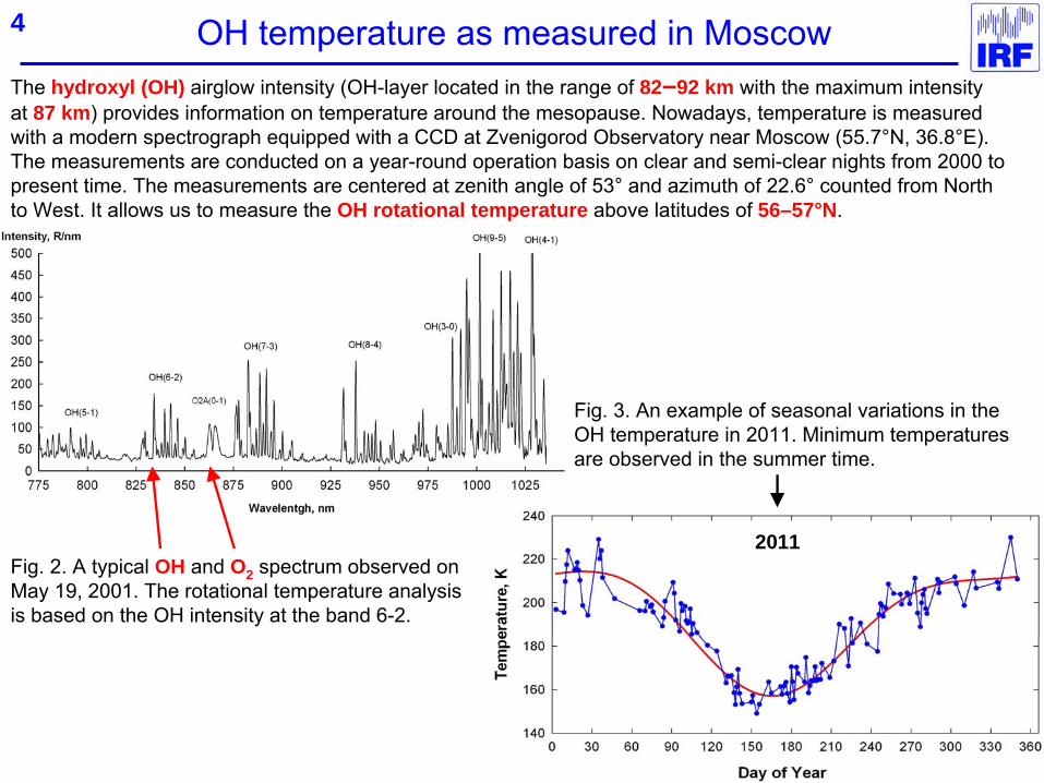
The hydroxyl (OH) airglow intensity (OH-layer located in the range of 82–92 km with the maximum intensity at 87 km) provides information on temperature around the mesopause. Nowadays, temperature is measured with a modern spectrograph equipped with a CCD at Zvenigorod
Observatory near Moscow (55.7°N, 36.8°E). The measurements are conducted on a year-round operation basis on clear and semi-clear nights from 2000 to present time. The measurements are centered at zenith angle of 53°
and azimuth of 22.6°
counted from North to West. It allows us to measure the OH rotational temperature above latitudes of 56–57°N.
OH temperature as measured in Moscow
Fig. 2. A typical OH and O2 spectrum observed on May 19, 2001. The rotational temperature analysis is based on the OH intensity at the band 6-2.
Fig. 3. An example of seasonal variations in the OH temperature in 2011. Minimum temperatures are observed in the summer time.
2011
4

2000 2001 2002 2003 2004 2005 2006 2007 2008 2009 2010 2011 2012158
159
160
161
162
163
164
165
166
Years
Tem
pera
ture
[ K
]
Model:Y= − 0.351±0.760⋅ t − 0.541±4.186 ⋅ Lyα + 165.5
OH Temperature data
All the analyzed parameters (temperature or NLC quantities) are fitted with a two-dimensional regression model which includes dependence on time and solar cycle, which is represented by the Lyman-alpha flux (Lyα
):
Y= b1
·(t–t0
) + b2
·Lyα
(t–lag) + b3
where are b1, b2 are fit parameters for the time trend and for the Lyα
flux, respectively, b3 is the fit constant, t0 is the start year of the time series, lag is the phase lag between the solar cycle and NLC or T data sets.
OH temperature trend in the summer mesopause at 56-57°N
Fig. 4. The OH minimum temperatures for summer seasons from 2000 to 2011 (blue curve) and its two-dimensional regression model (red curve). Lag=0 year.
5

3.4 3.6 3.8 4 4.2 4.4 4.6 4.8 5 5.2 5.4160
161
162
163
164
165
166
167
Tem
pera
ture
[ K
]
Moscow OH temperature vs. solar cycle. Time dependece has been removed
Lyα flux [1011 ph /cm2 /s]
2000 2001 2002 2003 2004 2005 2006 2007 2008 2009 2010 2011 2012158
160
162
164
166
168
170
Years
Tem
pera
ture
[ K
]
Moscow OH temperature vs. time. Solar cycle has been removed
Y= −0.351 ± 0.381⋅ t
Y= −0.541 ± 2.095 ⋅Lyα
OH temperature trend in the summer mesopause at 56-57°N
Fig. 5. The upper panel: OH temperature vs. the Lyα
flux, with the time dependence being subtracted. The lower panel: OH temperature vs. time, with the solar cycle being subtracted.
It is seen that the summer temperature dependence on solar flux is close to zero, and the linear dependence on time is slightly negative (–0.35 K/yr) and it lacks statistical significance.
6

1960 1965 1970 1975 1980 1985 1990 1995 2000 2005 20100
5
10
15
20
25
30
NLC
cas
es
Years
Moscow NLC observations
Model: Y= 0.227 ± 0.110⋅ t −3.706 ± 2.152⋅ Lyα + 23.5
Moscow NLC trend analysis for 1962-2011
Fig. 7 shows
the Moscow NLC observations, starting from 1962 (black curve), and its regression model (blue curve). The found regression coefficients are highly significant. However, it is evident there are two different statistics: before and after 2005. The 2005 year is the start of the digital epoch
in NLC observations in Moscow. After establishing automated digital cameras we are able to monitor the twilight sky longer period, from the end of May to the middle of August, compared to the period of visual observations conducted from the end of May to the middle of July. Also, digital images allow us to better identify NLC under complex weather conditions. That is why the number of NLC events starting from 2005 is greater than those before the digital epoch. To take into
account these different statistics, we apply a procedure of normalization by the number of clear and semi-clear weather nights
during an NLC season.
7
1. Port Glasgow (Scotland). 2. Athabasca (Canada)3. Kamchatka (Russia). 4. Novosibirsk (Russia). 5. Moscow (Russia). 6. Vilnius (Lithuania). 7. Århus
(Denmark).
Fig. 6.

1960 1965 1970 1975 1980 1985 1990 1995 2000 2005 2010−0.4
−0.3
−0.2
−0.1
0
0.1
0.2
0.3
0.4
rela
tive
NLC
num
ber
Years
Moscow NLC relative number, normalized by the number of clear nights. Solar cycle has been removed
Y= 0.0002 ± 0.0031⋅ t
Moscow NLC trend analysis for 1962-2011
Fig. 8 shows the Moscow NLC relative number, normalized by the number of clear and semi-clear weather nights. The solar cycle has been subtracted with correlation lag equal to 1 year. The long-term trend in relative NLC occurrence frequency equals to
zero.
8

1960 1965 1970 1975 1980 1985 1990 1995 2000 2005 2010
0
100
200
300
400
500
600
700
Inte
gral
NLC
brig
htne
ss [m
arks
]
Moscow NLC brightness observations
1960 1965 1970 1975 1980 1985 1990 1995 2000 2005 2010−6
−4
−2
0
2
4
6
8
10
Years
Rel
ativ
e br
ight
ness
of N
LC [r
el. m
arks
] Relative NLC brightness, normalized by the number of clear nights. Solar cycle has been removed
Model: Y= 4.813±2.096⋅ t −76.101±41.000⋅ Lα + 415.3
Y= 0.057 ± 0.072 ⋅ t
Moscow NLC trend analysis for 1962-2011
Fig. 9 shows the Moscow NLC brightness which is traditionally visually estimated on a 5-point scale. This is so called the integral NLC brightness that is
a total brightness for a whole NLC season. There is a significant positive trend as seen in the upper panel. Again, there are two different
statistics before and after 2005. However, after normalizing by the number of clear and semi-clear weather nights we arrive at a slight positive trend (0.057 Mark/yr) which lacks statistical significance (lower panel).
9

1990 1992 1994 1996 1998 2000 2002 2004 2006 2008 2010 201212
16
20
24
28
32
36
40
NLC
cas
es
Years
Lithuanian NLC observations, all brightness
Model: Y= 0.109 ± 0.345 ⋅t −0.762 ± 2.953 ⋅Lyα +57.5
Lithuanian NLC trend analysis
Fig. 10 illustrates the number of all NLC displays for 20 years from 1991 to 2011
(black curve), NLC data include a weather corrected factor. The blue line is its regression model which includes dependence on time and solar cycle. The black line is a linear dependence on time, which shows a rather strong positive trend.
The Lithuanian data base consists of two data sets:1. Observations of NLCs of all brightnesses, i.e. all observed NLCs from 1991 to 2011.2. Observations of VERY BRIGHT NLCs from
1973 to 2011.
10

1990 1992 1994 1996 1998 2000 2002 2004 2006 2008 2010 2012−6
−4
−2
0
2
4
6
8
10
12
NLC
cas
es
Years
Lithuanian NLC observations of all brightness. Solar cycle has been removed.
Y= 0.109 ± 0.291⋅ t
Lithuanian NLC trend analysis
Fig. 11 illustrates the long-term trend in the Lithuanian observations of NLCs of all brightnessesfrom 1991 to 2011. The black line is the regression model after subtracting the solar cycle.
One can see that there is a small positive trend (0.11 N/yr) which lacks statistical significance.
11

1970 1975 1980 1985 1990 1995 2000 2005 2010−2
0
2
4
6
8
10
NLC
cas
es
very bright Lithuanian NLC
Year
Model: Y= 0.039 ± 0.058⋅t −2.143 ± 0.902 ⋅Lyα + 11.3
Lithuanian NLC trend analysis
Fig. 12 illustrates time series of the Lithuanian observations of VERY BRIGHT NLCs from 1973 to 2011 (black curve). The blue line is the 2D regression model which includes the dependence on time and solar cycle. The black line is a linear dependence on time, which shows a rather strong positive trend.
12

1970 1975 1980 1985 1990 1995 2000 2005 2010−4
−3
−2
−1
0
1
2
3
4
5
6
NLC
cas
es
Years
Very bright Lithuanian NLC. Solar cycle has been removed.
Y= 0.039 ± 0.056 ⋅t
Lithuanian NLC trend analysis
Fig. 13 shows the long-term trend in the Lithuanian observations of VERY BRIGHT NLCs. The black line is the regression model after subtracting the solar component.
It is evident that
there is a slight positive trend (0.04 N/yr), however, it has no statistical significance.
13

How our data is relevant for long-term PMC modeling
Modeling of PMC trends is a function of the temperature trend and water vapor trend around the summer mesopause, that is:
PMCtrend
= f (Ttrend
, H2Otrend
)
If a PMC model is flexible to atmospheric conditions at different latitudes then:
► with OH summer temperature measurements
we can contribute to the PMC/NLC modeling at midlatitudes
of 56-57°N
during several decades;
► it would be worth running such a PMC model for latitudes of 57-60°N
(where NLCs are commonly observed) for which we have reliable long-term NLC data. Our NLC data sets could be used as a reference base
for comparison with the output of a PMC model.
14

Conclusions on long-term trend analysis around the summer mesopause
1. There exists a slight negative trend (-0.35 K/yr) in minimum temperatures in the summer time at ~87 km
as measured by the OH spectrometer in Moscow from 2000 to 2011. However, the trend lacks statistical significance. The long-term trend
in the summer mesopause temperature is about zero
at around 87 km from 1960 to 1996
, and the T-trend is slightly negative at around 80 km from 1969 to 1996. The last one has been derived from rocket measurements in Volgograd (Russia) by Golitsyn et al. (1996), Semenov et al. (2002). All these trends are valid for midlatitudes
only.
2. There is no statistically significant long-term trend in the Moscow NLC observations from 1962 to 2011. This is valid both for time series of the NLC number and NLC brightness estimations. Please note that the Moscow ground-based NLC observations are longer than any satellite time series
of PMCs. It is possible to combine time series of NLC observed visually (the old epoch) and NLC registered with digital cameras (the digital epoch). The correct procedure is to normalize NLC quantities by the number of clear and semi-clear weather nights, which does not provide more scattering of the data points.
3. The statistical analysis of the Lithuanian data sets demonstrates that there is a slight long-term positive trend (0.11 N/yr) in NLC observations of all brightnesses
from 1991 to 2011
as well as in very bright NLCs (0.04 N/yr) from 1973 to 2011. However, both trends lack statistical significance.
4. Zero OH temperature trend in the summer mesopause at ~87 km
probably explains zero trends in the NLC occurrence frequency. At the same time, a slight negative temperature trend at 80 km
might explain positive trends (0.04 N/yr) in very bright NLCs, by the Lithuanian data,
and in the NLC brightness (0.057 Mark/yr), by the Moscow data. The reason is that the brightest NLCs are composed of largest particles, which build at the lowermost level (at 80-81 km). The positive long-term trend in water vapor around the summer mesopause (if exists) does not provide a plausible explanation on it. In case of existence of long-term trend in water vapor we should see the increase both in the NLC occurrence frequency and
in the NLC brightness.
5. Our OH summer temperature measurements
can be used as the input for PMC/NLC modeling at midlatitudes
of 56-57°N. It would be worth running such a PMC model for latitudes of 57-60°N
for which we have reliable long-
term NLC data. Our NLC data could be used as a reference base for comparison with the output of a PMC model.
15

THANKS!
The PMC/NLC and T-trend analysis …
to be continued
16

−10 −8 −6 −4 −2 0 2 4 6 8 10−0.6
−0.5
−0.4
−0.3
−0.2
−0.1
0
0.1
0.2
0.3
0.4
Lag [ years ]
Cor
r. c
oeff.
Cross−correlation between the NLC number and solar cycle
NLC numberrelative NLC number
Additional slides in case of available time or for questions
Cross-correlation dependence between the Moscow NLC number and solar cycle (solid line), and between the relative NLC number and solar cycle (dashed line).
17
Additional slides in case of available time or for questions
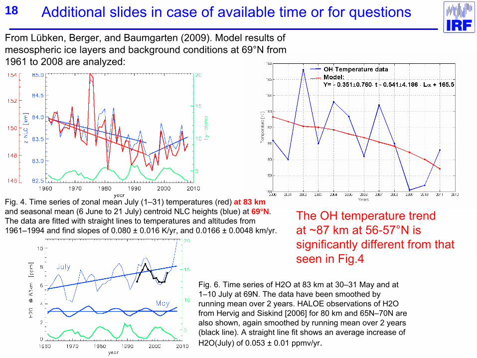
Fig. 4. Time series of zonal mean July (1–31) temperatures (red) at 83 km and seasonal mean (6 June to 21 July) centroid
NLC heights (blue) at 69°N. The data are fitted with straight lines to temperatures and altitudes from 1961–1994 and find slopes of 0.080 ±
0.016 K/yr, and 0.0166 ±
0.0048 km/yr.
Fig. 6. Time series of H2O at 83 km at 30–31 May and at 1–10 July at 69N. The data have been smoothed by running mean over 2 years. HALOE observations of H2O from Hervig
and Siskind
[2006] for 80 km and 65N–70N are also shown, again smoothed by running mean over 2 years (black line). A straight line fit shows an average increase of H2O(July) of 0.053 ±
0.01 ppmv/yr.
From Lübken, Berger, and Baumgarten
(2009). Model results of mesospheric ice layers and background conditions at 69°N from 1961 to 2008 are analyzed:
The OH temperature trend at ~87 km at 56-57°N is significantly different from that seen in Fig.4
18

Additional slides in case of available time or for questions
Dalin, P., Kirkwood, S., Andersen, H., Hansen, O., Pertsev, N., Romejko, V.: Comparison of long-term Moscow and Danish NLC observations: statistical results, Annales Geophysicae, 24, 2841-2849, 2006.
Dubietis, A., Dalin, P., Balciunas, R., Cernis, K.: Observations of noctilucent clouds from Lithuania, J. Atmos. Sol-Terr. Phys., 72, 14-15, 1090-1099, doi:10.1016/j.jastp.2010.07.004, 2010.
Golitsyn, G.S., Semenov, A.I. ,Shefov, N.N., Fishkova, L.M., Lysenko, E.V., and Perov, S.P.: Long-term temperature trends in the middle and upper atmosphere. Geophys. Res. Lett., 23, 14, 1741-1744, 1996.
Kirkwood, S., Dalin, P., Réchou, A.: Noctilucent clouds observed from the UK and Denmark –
trends and variations over 43 years, Annales Geophysicae, 26, 1243-1254, 2008.
Lübken, F.-J., Berger, U., and Baumgarten, G.:
Stratospheric and solar cycle effects on long-term variability ofmesospheric ice clouds, J. Geophys. Res., 114, D00I06, doi:10.1029/2009JD012377, 2009.
Perminov, V. and Pertsev, N.: Seasonal features of the response of temperature and emission intensities in the mesopause on solar activity variations. Geomagnetism and Aeronomy, 49, 1, 91-99, 2009.
Pertsev, N. and Perminov, V.: Response of the mesopause airglow to solar activity inferred from measurements at Zvenigorod, Russia. Annales Geophysicae, 26, 1049–1056, 2008.
Romejko, V.A., Dalin, P.A., Pertsev, N.N.: Forty years of noctilucent cloud observations near Moscow: database and simple statistics, J. Geophys. Res., 108, D8, 8443, 2003.
Semenov, A.I.: Long-term temperature trends for different seasons by hydroxyl emission. Physics and Chemistry of the Earth (B), 25, 5-6, 525-529, 2000.
Semenov, A.I., Shefov, N.N., Lysenko, E.V., Givishvili, G.V., Tikhonov, A.V.: The season peculiarities of behaviour
of the long-term temperature trends in the middle atmosphere on the mid-latitudes. Physics and Chemistry of the Earth, 27, 529–534, 2002.
Shettle, E.P., DeLand, M.T., Thomas, G.E., and Olivero, J.J.: Long term variations in the frequency of polar mesospheric clouds in the Northern Hemisphere from SBUV, Geophys. Res. Lett., 36, 2803–2806, doi:10.1029/2008GL036048, 2009.
Relevant publications:
19