HAL Id: hal-00819094https://hal.archives-ouvertes.fr/hal-00819094

Submitted on 3 May 2013

HAL is a multi-disciplinary open accessarchive for the deposit and dissemination of sci-entific research documents, whether they are pub-lished or not. The documents may come fromteaching and research institutions in France orabroad, or from public or private research centers.

L’archive ouverte pluridisciplinaire HAL, estdestinée au dépôt et à la diffusion de documentsscientifiques de niveau recherche, publiés ou non,émanant des établissements d’enseignement et derecherche français ou étrangers, des laboratoirespublics ou privés.

On the linear combination of the Gaussian and student’st random field and the integral geometry of its excursion

setsOla Ahmad, Jean-Charles Pinoli

To cite this version:Ola Ahmad, Jean-Charles Pinoli. On the linear combination of the Gaussian and student’s t randomfield and the integral geometry of its excursion sets. Statistics and Probability Letters, Elsevier, 2013,83, pp.559-567. <10.1016/j.spl.2012.10.022>. <hal-00819094>

On the linear combination of the Gaussian and student’s t

random field and the integral geometry of its excursion sets

Ola Ahmad∗, Jean-Charles Pinoli∗

LGF, UMR CNRS 5146

Ecole Nationale Superieure des Mines de Saint-Etienne

158 cours Fauriel, F-42023 Saint-Etienne cedex 2, France

Abstract

In this paper, a random field, denoted by GT νβ , is defined from the linear combination

of two independent random fields, one is a Gaussian random field and the second is

a student’s t random field with ν degrees of freedom scaled by β. The goal is to give

the analytical expressions of the expected Euler-Poincare characteristic of the GT νβ

excursion sets on a compact subset S of R2. The motivation comes from the need to

model the topography of 3D rough surfaces represented by a 3D map of correlated

and randomly distributed heights with respect to a GT νβ random field. The analytical

and empirical Euler-Poincare characteristic are compared in order to test the GT νβ

model on the real surface.

Keywords: Gaussian random field, Student’s t random field, Excursion sets,

Minkowski functionals, Euler-Poincare characteristic

∗Corresponding author.Email address: ahmad@emse.fr (Ola Ahmad)

Preprint submitted to Statistics & Probability Letters October 25, 2012

1. Introduction

The motivation of studying the linear combination between the Gaussian and the

student’s t random fields, GT νβ , comes from the need to model some examples of 3D

rough engineering surfaces used in biomedical and material science applications.

Studying the spatial evolution of a surface or the deformation of its peaks requires

combination between different types of random fields. This combination might in-

crease the flexibility of the model, since it defines further statistical parameters that

enable describing the shape of the height’s distribution, (i.e. the skewness, the kur-

tosis,...etc.), which could interpret the functionality of such surfaces during certain

phenomenons, when they cannot be involved by only the Gaussian random fields.

Gaussian and several non-Gaussian random fields, including, without limitation,

χ2, F , student’s t and Hotelling’s t2 random fields, have been studied by (Adler, 1981;

Adler and Taylor, 2007; Alder and Taylor, 2003; Cao and Worsley, 2001; Worsley,

1995) in order to detect the p-value of the local maxima of a random field inside a

searching region that correspond to a certain activation in the brain or for searching

certain anomalies in medical imaging applications. For this aim, the integral geomet-

ric characteristics of the excursion sets of such random fields have been investigated

in (Adler and Taylor, 2011; Adler, 1981; Cao, 1997; Worsley, 1995). The excursion

sets are defined as the upper sets that result from thresholding the random field at

a given level h. For example, the excursion set at a height level h of a 3D surface

defined on a two-dimensional space will result from hitting the surface heights with

a plane at the level h. Thus, all the heights that exceed the threshold h will belong

to this excursion set. The integral geometry of the excursion sets is of great interest,

since it defines their Euler, or Euler-Poincare characteristic, which counts, on a com-

2

pact subset of two dimensions, the number of connected components of the excursion

set, minus the number of holes. This characteristic function enables detecting the

peaks and the valleys elevations on 3D rough surfaces, and so, it describes the surface

roughness.

In this paper, we are interested in studying the linear combination of a station-

ary Gaussian random field, denoted by G, and a non-Gaussian random field, namely

student’s t random field with ν degrees of freedom, denoted by T ν , i.e., the sum

G(x) + βT ν(x), where x stands for the spatial location that belongs to a subset S

of R2. This random field will be denoted by GT νβ . The goal is to introduce the sta-

tionary GT νβ random field, and to calculate analytically the expected Euler-Poincare

characteristic of its excursion set on a rectangle of R2.

The paper is organized as follows. Firstly, the GT νβ random field is defined, (sec-

tion 2), with its distribution function. Secondly, the expected Euler-Poincare char-

acteristic of the GT νβ excursion sets is expressed analytically on R

2 (section 3) . An

application is reported on a 3D rough surface, (section 4), in order to test the GT νβ

random field on the height’s map, and to describe the surface roughness.

2. GTνβ

random fields

2.1. Notation

Let Y (x) be a real-valued random field, {Y = Y (x), x ∈ S}, represented at a point

x in a compact subset S of the Euclidean space Rd, with mean µY and variance σ2

Y .

The N ×N covariance matrix of any arbitrary finite collection

{Yi = Y (xi), i ≤ 1 ≤ N, xi ∈ S}, will be denoted by CY , where CY (i, j) = E[(Yi −µYi

)(Yj−µYj)], (i, j = 1, ..., N). The probability density function of Y , at any point x,

3

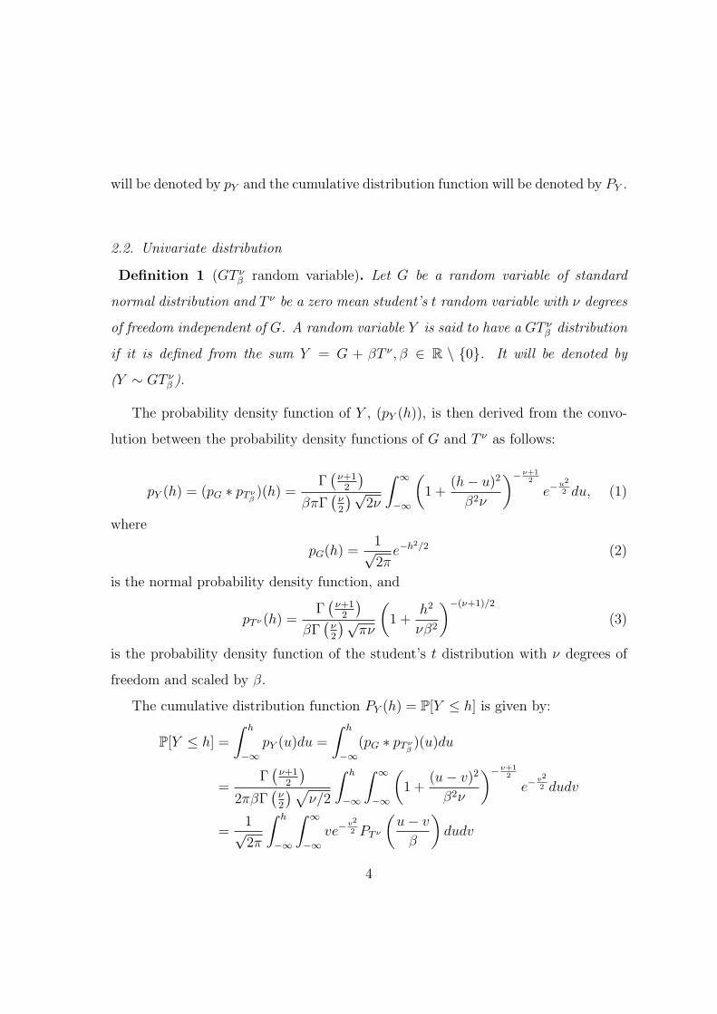
will be denoted by pY and the cumulative distribution function will be denoted by PY .

2.2. Univariate distribution

Definition 1 (GT νβ random variable). Let G be a random variable of standard

normal distribution and T ν be a zero mean student’s t random variable with ν degrees

of freedom independent of G. A random variable Y is said to have a GT νβ distribution

if it is defined from the sum Y = G + βT ν , β ∈ R \ {0}. It will be denoted by

(Y ∼ GT νβ ).

The probability density function of Y , (pY (h)), is then derived from the convo-

lution between the probability density functions of G and T ν as follows:

pY (h) = (pG ∗ pT νβ)(h) =

Γ(

ν+12

)

βπΓ(

ν2

)√2ν

∫ ∞

−∞

(

1 +(h− u)2

β2ν

)− ν+12

e−u2

2 du, (1)

where

pG(h) =1√2π

e−h2/2 (2)

is the normal probability density function, and

pT ν (h) =Γ(

ν+12

)

βΓ(

ν2

)√πν

(

1 +h2

νβ2

)−(ν+1)/2

(3)

is the probability density function of the student’s t distribution with ν degrees of

freedom and scaled by β.

The cumulative distribution function PY (h) = P[Y ≤ h] is given by:

P[Y ≤ h] =

∫ h

−∞

pY (u)du =

∫ h

−∞

(pG ∗ pT νβ)(u)du

=Γ(

ν+12

)

2πβΓ(

ν2

)√

ν/2

∫ h

−∞

∫ ∞

−∞

(

1 +(u− v)2

β2ν

)− ν+12

e−v2

2 dudv

=1√2π

∫ h

−∞

∫ ∞

−∞

ve−v2

2 PT ν

(

u− v

β

)

dudv

4

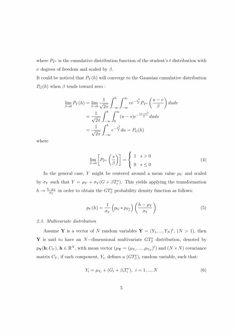
where PT ν is the cumulative distribution function of the student’s t distribution with

ν degrees of freedom and scaled by β.

It could be noticed that PY (h) will converge to the Gaussian cumulative distribution

PG(h) when β tends toward zero :

limβ→0

PY (h) = limβ→0

1√2π

∫ h

−∞

∫ ∞

−∞

ve−v2

2 PT ν

(

u− v

β

)

dudv

=1√2π

∫ h

−∞

∫ ∞

0

(u− s)e−(u−s)2

2 duds

=1√2π

∫ h

−∞

e−u2

2 du = PG(h)

where

limβ→0

[

PT ν

(

s

β

)]

=

1 s > 0

0 s ≤ 0(4)

In the general case, Y might be centered around a mean value µY and scaled

by σY such that Y = µY + σY (G + βT νs ). This yields applying the transformation

h → h−µY

σYin order to obtain the GT ν

β probability density function as follows:

pY (h) =1

σY

(

pG ∗ pT νβ

)

(

h− µY

σY

)

(5)

2.3. Multivariate distribution

Assume Y is a vector of N random variables Y = (Y1, ..., YN )t, (N > 1), then

Y is said to have an N−dimensional multivariate GT νβ distribution, denoted by

pY(h;CY ), h ∈ RN , with mean vector (µY = (µY1 , ..., µYN

)t) and (N ×N) covariance

matrix CY , if each component, Yi, defines a (GT νβ )i random variable, such that:

Yi = µYi+ (Gi + βiT

νi ), i = 1, ..., N (6)

5

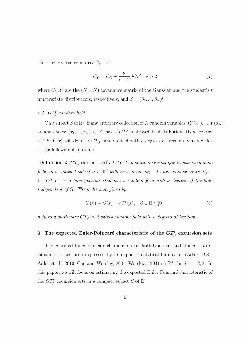
then the covariance matrix CY is:

CY = CG +ν

ν − 2βCβt, ν > 2 (7)

where CG, C are the (N ×N) covariance matrix of the Gaussian and the student’s t

multivariate distributions, respectively, and β = (β1, ..., βN )t.

2.4. GT νβ random field

On a subset S of Rd, if any arbitrary collection ofN random variables, (Y (x1), ..., Y (xN))

at any choice (x1, ..., xN ) ∈ S, has a GT νβ multivariate distribution, then for any

x ∈ S, Y (x) will define a GT νβ random field with ν degrees of freedom, which yields

to the following definition :

Definition 2 (GT νβ random field). Let G be a stationary isotropic Gaussian random

field on a compact subset S ⊂ Rd with zero mean, µG = 0, and unit variance σ2

G =

1. Let T ν be a homogeneous student’s t random field with ν degrees of freedom,

independent of G. Then, the sum given by:

Y (x) = G(x) + βT ν(x), β ∈ R \ {0} (8)

defines a stationary GT νβ real-valued random field with ν degrees of freedom.

3. The expected Euler-Poincare characteristic of the GTνβ

excursion sets

The expected Euler-Poincare characteristic of both Gaussian and student’s t ex-

cursion sets has been expressed by its explicit analytical formula in (Adler, 1981;

Adler et al., 2010; Cao and Worsley, 2001; Worsley, 1994) on Rd, for d = 1, 2, 3. In

this paper, we will focus on estimating the expected Euler-Poincare characteristic of

the GT νβ excursion sets in a compact subset S of R2.

6

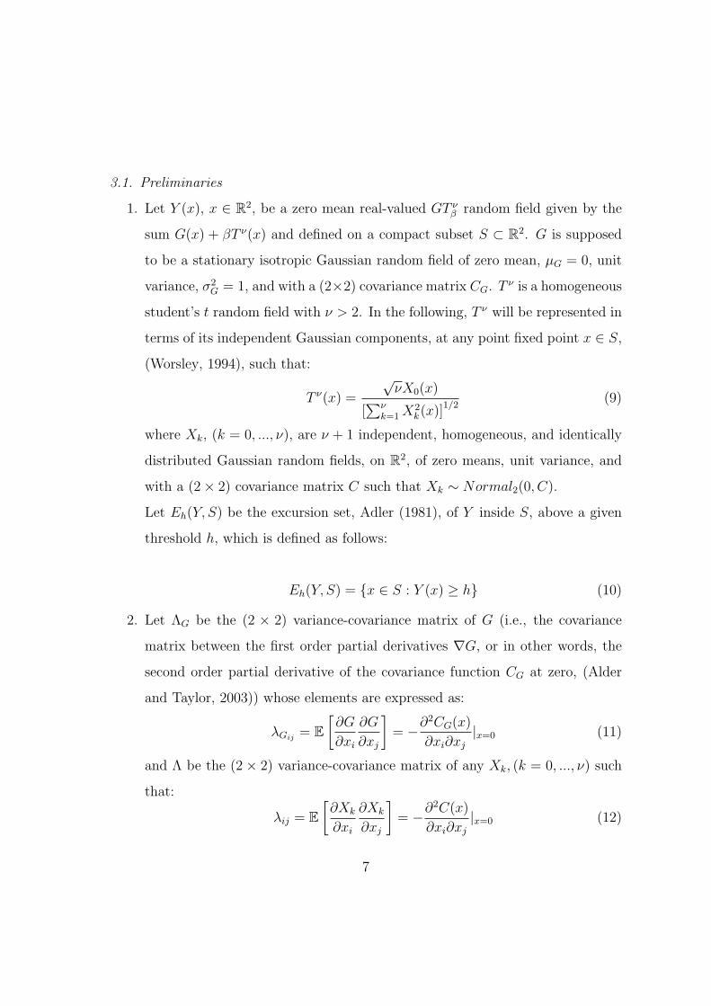
3.1. Preliminaries

1. Let Y (x), x ∈ R2, be a zero mean real-valued GT ν

β random field given by the

sum G(x) + βT ν(x) and defined on a compact subset S ⊂ R2. G is supposed

to be a stationary isotropic Gaussian random field of zero mean, µG = 0, unit

variance, σ2G = 1, and with a (2×2) covariance matrix CG. T

ν is a homogeneous

student’s t random field with ν > 2. In the following, T ν will be represented in

terms of its independent Gaussian components, at any point fixed point x ∈ S,

(Worsley, 1994), such that:

T ν(x) =

√νX0(x)

[∑ν

k=1X2k(x)]

1/2(9)

where Xk, (k = 0, ..., ν), are ν + 1 independent, homogeneous, and identically

distributed Gaussian random fields, on R2, of zero means, unit variance, and

with a (2× 2) covariance matrix C such that Xk ∼ Normal2(0, C).

Let Eh(Y, S) be the excursion set, Adler (1981), of Y inside S, above a given

threshold h, which is defined as follows:

Eh(Y, S) = {x ∈ S : Y (x) ≥ h} (10)

2. Let ΛG be the (2 × 2) variance-covariance matrix of G (i.e., the covariance

matrix between the first order partial derivatives ∇G, or in other words, the

second order partial derivative of the covariance function CG at zero, (Alder

and Taylor, 2003)) whose elements are expressed as:

λGij= E

[

∂G

∂xi

∂G

∂xj

]

= −∂2CG(x)

∂xi∂xj

|x=0 (11)

and Λ be the (2× 2) variance-covariance matrix of any Xk, (k = 0, ..., ν) such

that:

λij = E

[

∂Xk

∂xi

∂Xk

∂xj

]

= −∂2C(x)

∂xi∂xj

|x=0 (12)

7

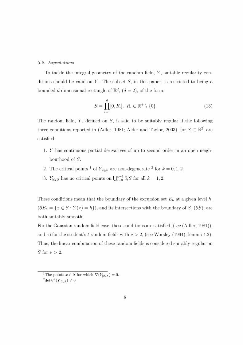
3.2. Expectations

To tackle the integral geometry of the random field, Y , suitable regularity con-

ditions should be valid on Y . The subset S, in this paper, is restricted to being a

bounded d-dimensional rectangle of Rd, (d = 2), of the form:

S =d∏

i=1

[0, Ri], Ri ∈ R+ \ {0} (13)

The random field, Y , defined on S, is said to be suitably regular if the following

three conditions reported in (Adler, 1981; Alder and Taylor, 2003), for S ⊂ R2, are

satisfied:

1. Y has continuous partial derivatives of up to second order in an open neigh-

bourhood of S.

2. The critical points 1 of Y|∂kS are non-degenerate 2 for k = 0, 1, 2.

3. Y|∂kS has no critical points on⋃k−1

i=0 ∂iS for all k = 1, 2.

These conditions mean that the boundary of the excursion set Eh at a given level h,

(∂Eh = {x ∈ S : Y (x) = h}), and its intersections with the boundary of S, (∂S), are

both suitably smooth.

For the Gaussian random field case, these conditions are satisfied, (see (Adler, 1981)),

and so for the student’s t random fields with ν > 2, (see Worsley (1994), lemma 4.2).

Thus, the linear combination of these random fields is considered suitably regular on

S for ν > 2.

1The points x ∈ S for which ∇(Y|∂kS) = 0.

2det∇2(Y|∂kS) 6= 0

8

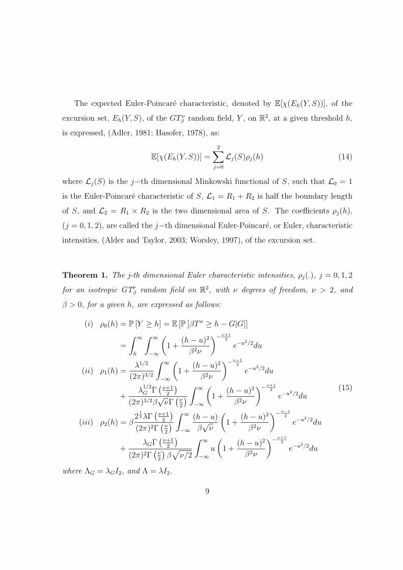
The expected Euler-Poincare characteristic, denoted by E[χ(Eh(Y, S))], of the

excursion set, Eh(Y, S), of the GT νβ random field, Y , on R

2, at a given threshold h,

is expressed, (Adler, 1981; Hasofer, 1978), as:

E[χ(Eh(Y, S))] =2

∑

j=0

Lj(S)ρj(h) (14)

where Lj(S) is the j−th dimensional Minkowski functional of S, such that L0 = 1

is the Euler-Poincare characteristic of S, L1 = R1 + R2 is half the boundary length

of S, and L2 = R1 × R2 is the two dimensional area of S. The coefficients ρj(h),

(j = 0, 1, 2), are called the j−th dimensional Euler-Poincare, or Euler, characteristic

intensities, (Alder and Taylor, 2003; Worsley, 1997), of the excursion set.

Theorem 1. The j-th dimensional Euler characteristic intensities, ρj(.), j = 0, 1, 2

for an isotropic GTνβ random field on R

2, with ν degrees of freedom, ν > 2, and

β > 0, for a given h, are expressed as follows:

(i) ρ0(h) = P [Y ≥ h] = E [P [βT ν ≥ h−G|G]]

=

∫ ∞

h

∫ ∞

−∞

(

1 +(h− u)2

β2ν

)− ν+12

e−u2/2du

(ii) ρ1(h) =λ1/2

(2π)3/2

∫ ∞

−∞

(

1 +(h− u)2

β2ν

)− ν−12

e−u2/2du

+λ1/2G Γ

(

ν+12

)

(2π)3/2β√νΓ

(

ν2

)

∫ ∞

−∞

(

1 +(h− u)2

β2ν

)− ν+12

e−u2/2du

(iii) ρ2(h) = β2

12λΓ

(

ν+12

)

(2π)2Γ(

ν2

)

∫ ∞

−∞

(h− u)

β√ν

(

1 +(h− u)2

β2ν

)− ν−12

e−u2/2du

+λGΓ

(

ν+12

)

(2π)2Γ(

ν2

)

β√

ν/2

∫ ∞

−∞

u

(

1 +(h− u)2

β2ν

)− ν+12

e−u2/2du

(15)

where ΛG = λGI2, and Λ = λI2.

9

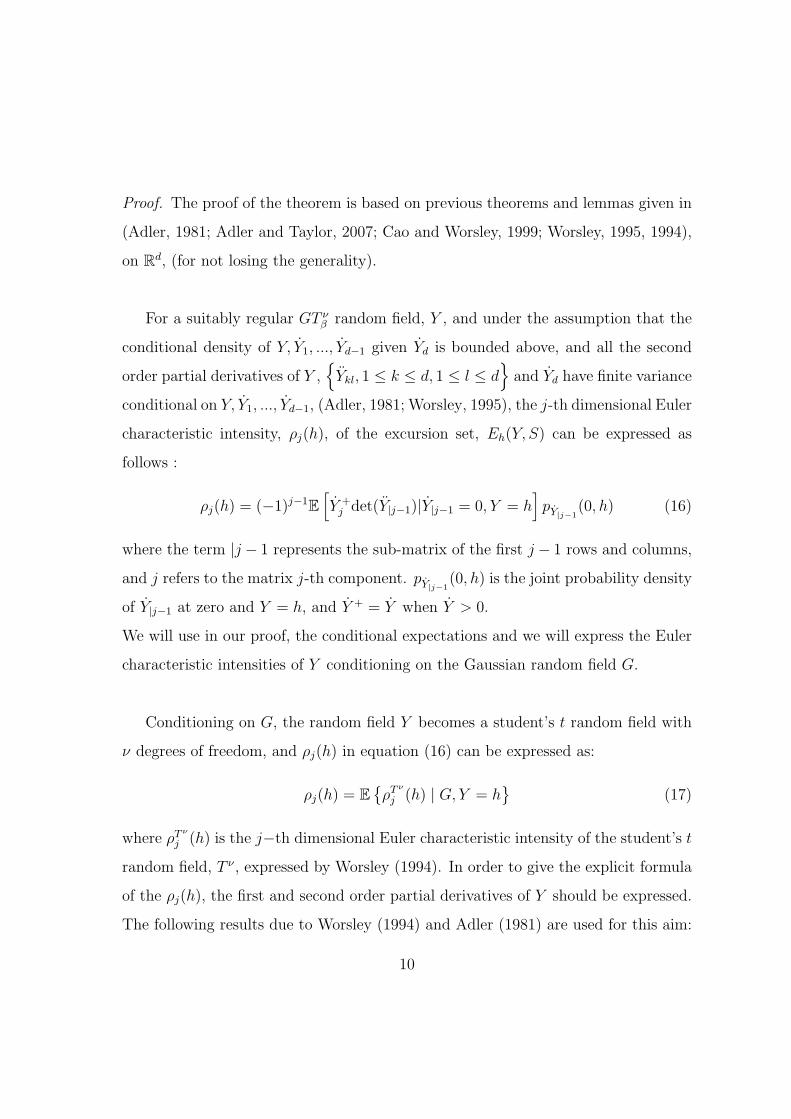
Proof. The proof of the theorem is based on previous theorems and lemmas given in

(Adler, 1981; Adler and Taylor, 2007; Cao and Worsley, 1999; Worsley, 1995, 1994),

on Rd, (for not losing the generality).

For a suitably regular GT νβ random field, Y , and under the assumption that the

conditional density of Y, Y1, ..., Yd−1 given Yd is bounded above, and all the second

order partial derivatives of Y ,{

Ykl, 1 ≤ k ≤ d, 1 ≤ l ≤ d}

and Yd have finite variance

conditional on Y, Y1, ..., Yd−1, (Adler, 1981; Worsley, 1995), the j-th dimensional Euler

characteristic intensity, ρj(h), of the excursion set, Eh(Y, S) can be expressed as

follows :

ρj(h) = (−1)j−1E

[

Y +j det(Y|j−1)|Y|j−1 = 0, Y = h

]

pY|j−1(0, h) (16)

where the term |j − 1 represents the sub-matrix of the first j − 1 rows and columns,

and j refers to the matrix j-th component. pY|j−1(0, h) is the joint probability density

of Y|j−1 at zero and Y = h, and Y + = Y when Y > 0.

We will use in our proof, the conditional expectations and we will express the Euler

characteristic intensities of Y conditioning on the Gaussian random field G.

Conditioning on G, the random field Y becomes a student’s t random field with

ν degrees of freedom, and ρj(h) in equation (16) can be expressed as:

ρj(h) = E{

ρTν

j (h) | G, Y = h}

(17)

where ρTν

j (h) is the j−th dimensional Euler characteristic intensity of the student’s t

random field, T ν , expressed by Worsley (1994). In order to give the explicit formula

of the ρj(h), the first and second order partial derivatives of Y should be expressed.

The following results due to Worsley (1994) and Adler (1981) are used for this aim:

10

Lemma 1 (Adler (1981)). Let G be a Gaussian random field, (at any fixed point

x ∈ S), then,

G ∼ Normald(0,ΛG) independent of G and G

Conditioning on G,

G | G ∼ Normald×d(−GΛG,M(ΛG))

where M(ΛG) = Cov(∇2G | G) is (d× d) symmetric.

Lemma 2 (Worsley (1994)). The first and second order partial derivatives of the

student’s t random field with ν degrees of freedom, T ν, (at any fixed point x), can be

expressed in term of independent random random variables as follows:

T ν = ν1/2(1 + (T ν)2/ν)W−1/2z1

T ν = ν1/2(1 + (T ν)2/ν)W−1{−ν−1/2T ν(Q− 2z1zt1)− z1z

t2 − z2z

t1 +W 1/2H}

where W ∼ χ2ν+1, z1, z2 ∼ Normald(0,Λ), Q ∼ Wishartd(Λ, ν − 1) and H ∼

Normald×d(0,M(Λ)), all are independent.

Consequently, the first and second order partial derivatives of Y can be also

expressed in term of independent random variables, at any fixed point x ∈ S, as

follows:

Y = G+ βν1/2

(

1 +(Y −G)2

β2ν

)

W−1/2z1

Y = −GΛG + V

+ βν1/2(1 + (Y −G)2/ν)W−1{−β−1ν−1/2(Y −G)(Q− 2z1zt1)− z1z

t2 − z2z

t1 +W 1/2H}

where V ∼ Normald×d(0,M(ΛG)), and z1, z2,W,Q,H,G are all independent.

Conditioning on G, Y and W , the j−th dimensional Euler characteristic density

11

ρTν

j (h), in our case, becomes:

ρTν

j (h) = EW

{

E

[

(Y +j )det(−Y |j−1)|Y|j−1 = 0, G,W, Y = h

]

pY|j−1(0,W,G, h)

}

(18)

where pY|j−1(0,W,G, h) is the joint probability density of Y|j−1 at zero conditional on

Y = h, W and G.

The matrix Y|j−1 is the (j − 1) × (j − 1) of the Hessian matrix ∇2Y with re-

spect to x1, ..., xj−1. Considering the conditioning on Y1 = 0, ..., Yj−1 = 0, then,

the (j − 1) first order partial derivative components of both G and z1 are zeros, i.e.,

(G1 = 0, ...., Gj−1 = 0) and (z1(1) = 0, ..., z1(j−1)= 0), since G and z1 are independent.

Hence, Y|j−1 can be written as:

Y|j−1 = −GΛG+V +βν1/2(1+(Y −G)2/ν)W−1{−β−1ν−1/2(Y −G)Q+W 1/2H} (19)

Furthermore, Y|j−1 and Yj are also independent conditioning on G, Y , W and Y1 =

0, ..., Yj−1 = 0, so:

E

[

(Y +j )det(−Y |j−1)|Y|j−1 = 0, Y = h

]

= (−1)j−1×

E

[

(Y +j )|Y|j−1 = 0, G,W, Y = h

]

× E

[

det(Y|j−1)|Y|j−1 = 0, G,W, Y = h]

(20)

Since Y , conditioning on G, Y and W , is a linear mixture of two independent Gaus-

sian random fields, G and z1, with covariance matrix (ΛG+β2ν(

1 + (h−G)2

β2ν

)2

W−1Λ),

then:

E

[

(Y +j )|Y|j−1 = 0, G,W, Y = h

]

= (2π)−1/2

{

λG(j)+ β2ν

(

1 +(h−G)2

β2ν

)2

W−1λj

}1/2

(21)

where λG(j), λj are the j−th elements of the diagonal matrix ΛG,Λ, respectively, and

due to isotropy they become λG(j)= λG and λ = λj.

12

In order to calculate the determinant det(Y|j−1) conditional on Y = h, G, W and

Y|j−1 = 0, the matrix Y|j−1 is expressed as:

Y|j−1 = B + aQ+ bH (22)

where a = βν1/2(1 + (Y − G)2/ν)W−1{−β−1ν−1/2(Y − G), b = W 1/2 are con-

stants, B ∼ Normal(j−1)×(j−1)(−GΛG,M(ΛG)), Q ∼ Wishart(Λ, ν − 1), and H ∼Normal(j−1)×(j−1)(0,M(Λ)).

Firstly, let consider the orthogonal (j−1)× (j−1) matrix, U , such that U tΛ|j−1U =

Ij−1, then:

E

[

det(Y|j−1)|Yj−1 = 0, Y = h,G,W]

= E[det(B + aQ+ bH)] (23)

where B = U tBU , and B ∼ Normal(j−1)×(j−1)(−U tGΛGΛ−1U t,M(U tΛGΛ

−1U t)),

Q ∼ Wishart(I|j−1, ν − 1), and H ∼ Normal(j−1)×(j−1)(0,M(I)).

Using the lemmas in the appendix, (Appendix A), we obtain:

E

[

det(Y|j−1)|Yj−1 = 0, Y = h,G,W]

= detj−1(Λ)

⌊(j−1)/2⌋∑

i=0

(−1)i

2ii!b2i

j−1−2i∑

k=0

ak(

ν − 1

k

)

× [(2i+ k)!] detrj−1−2i−k(B)

(24)

where detk(.) stands for the matrix determinant of the first (k × k) elements, detrk

is the sum of the determinants of all k × k principal minors, and

detrm(B) = detm(ΛG)detm(Λ−1)

⌊(m)/2⌋∑

i=0

(−1)m−i(2i!)

2ii!Gm−2i (25)

13

Putting equations (25) and (24) together yields:

E

[

det(Y|j−1)|Yj−1 = 0, Y = h,G,W]

= detj−1(Λ)

⌊(j−1)/2⌋∑

i=0

(−1)i

2ii!b2i

j−1−2i∑

k=0

ak(

ν − 1

k

)

× detj−1−2i−k(ΛGΛ−1)

⌊(j−1−2i−k)/2⌋∑

l=0

(−1)j−1−2i−k−l

2ll!(2i+ 2l + k)!Gj−2i−k−2l−1

(26)

The joint probability density function of the (j−1) first derivatives of Y , pY|j−1(Y , G,W, h),

in equation (18), conditioning on G,W, Y = h, is a Gaussian joint probability den-

sity, (Y|j−1 ∼ Normalj−1(0,ΛG+β2ν(1+(h−G)2/β2ν)2W−1Λ)). Hence, the density

of Y|j−1 at zero becomes:

pY|j−1(0, G,W, h) = (2π)−

j−12

{

detj−1(ΛG + β2ν(1 + (h−G)2/β2ν)2W−1Λ)}− 1

2

(27)

Recall that W ∼ χ2ν+1 is a Chi-squared random field with ν + 1 degrees of freedom,

So, its moments are given such that:

E[W j] = 2jΓ((ν + 1)/2 + j)

Γ((ν + 1)/2)(28)

Since the j−th dimensional Euler characteristic intensity of the student’s t excursion

set conditioning on the Gaussian random field, ρTν

j (h), is known now, the j−th

dimensional Euler characteristic intensity of the GT νβ excursions set, ρj(h), can then

be expressed using equations (17) and (18), such that:

ρj(h) = (−1)j∫ ∞

−∞

pG(u)du×

EW

{

E

[

(Y +j )det(Y|j−1)|Y|j−1 = 0, G,W, Y = h

]

pY|j−1(0,W,G, h)

}

pY (h;G)

(29)

where pG(u) is the Gaussian probability density function, and PY (h;G) is the prob-

ability density function of Y at h conditional on G, which becomes a student’s t

14

density with ν degrees of freedom:

pY (h;G) =Γ(

ν+12

)

β√νΓ

(

ν2

)

(

1 +(h−G)2

β2ν

)− ν+12

(30)

For j = 2,

ρ2(h) = β2

12λXΓ

(

ν+12

)

(2π)2Γ(

ν2

)

∫ ∞

−∞

(h− u)

β√ν

(

1 +(h− u)2

β2ν

)− ν−12

e−u2/2du

+λGΓ

(

ν+12

)

(2π)2Γ(

ν2

)

β√

ν/2

∫ ∞

−∞

u

(

1 +(h− u)2

β2ν

)− ν+12

e−u2/2du

(31)

For j = 1, The expectation E[Y +j |Y|j−1 = 0, Y = h,G,W ] is expressed by using the

condition that stats Y > 0 when G > 0 and z1 > 0, such that:

E[Y +j |Y|j−1 = 0, Y = h,G,W ] = E[G+

j |Y|j−1 = 0, Y = h,G,W ]+

βν1/2

(

1 +(h−G)2

β2ν

)

W−1/2E[z+1j |Y|j−1 = 0, Y = h,G,W ]

= (2π)−1/2[λ1/2G + βν1/2

(

1 +(h−G)2

β2ν

)

W−1/2λ1/2]

(32)

Then

ρ1(h) = (2π)−1/2

∫ ∞

−∞

EW

[

λ1/2G + βν1/2

(

1 +(h−G)2

β2ν

)

W−1λ1/2

]

pY (h;G)pG(u)du

=λ1/2

(2π)3/2

∫ ∞

−∞

(

1 +(h− u)2

β2ν

)− ν−12

e−u2/2du

+λ1/2G Γ

(

ν+12

)

(2π)3/2βν1/2Γ(

ν2

)

∫ ∞

−∞

(

1 +(h− u)2

β2ν

)− ν+12

e−u2/2du

(33)

Finally, for j = 0, ρ0(h) = P[Y > h].

15

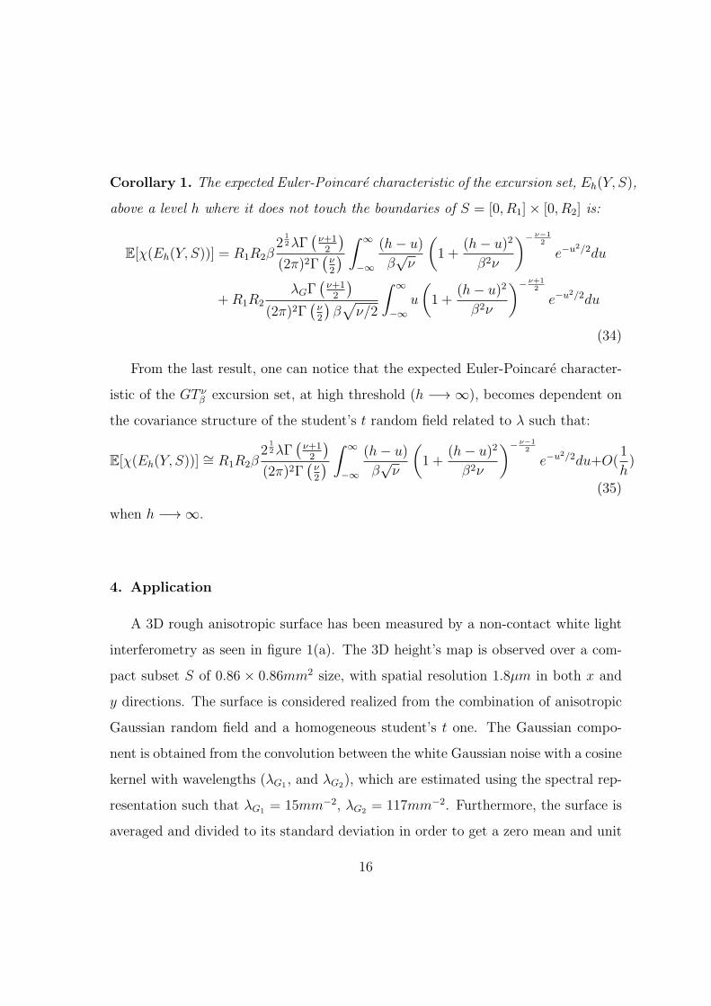
Corollary 1. The expected Euler-Poincare characteristic of the excursion set, Eh(Y, S),

above a level h where it does not touch the boundaries of S = [0, R1]× [0, R2] is:

E[χ(Eh(Y, S))] = R1R2β2

12λΓ

(

ν+12

)

(2π)2Γ(

ν2

)

∫ ∞

−∞

(h− u)

β√ν

(

1 +(h− u)2

β2ν

)− ν−12

e−u2/2du

+R1R2

λGΓ(

ν+12

)

(2π)2Γ(

ν2

)

β√

ν/2

∫ ∞

−∞

u

(

1 +(h− u)2

β2ν

)− ν+12

e−u2/2du

(34)

From the last result, one can notice that the expected Euler-Poincare character-

istic of the GT νβ excursion set, at high threshold (h −→ ∞), becomes dependent on

the covariance structure of the student’s t random field related to λ such that:

E[χ(Eh(Y, S))] ∼= R1R2β2

12λΓ

(

ν+12

)

(2π)2Γ(

ν2

)

∫ ∞

−∞

(h− u)

β√ν

(

1 +(h− u)2

β2ν

)− ν−12

e−u2/2du+O(1

h)

(35)

when h −→ ∞.

4. Application

A 3D rough anisotropic surface has been measured by a non-contact white light

interferometry as seen in figure 1(a). The 3D height’s map is observed over a com-

pact subset S of 0.86 × 0.86mm2 size, with spatial resolution 1.8µm in both x and

y directions. The surface is considered realized from the combination of anisotropic

Gaussian random field and a homogeneous student’s t one. The Gaussian compo-

nent is obtained from the convolution between the white Gaussian noise with a cosine

kernel with wavelengths (λG1 , and λG2), which are estimated using the spectral rep-

resentation such that λG1 = 15mm−2, λG2 = 117mm−2. Furthermore, the surface is

averaged and divided to its standard deviation in order to get a zero mean and unit

16

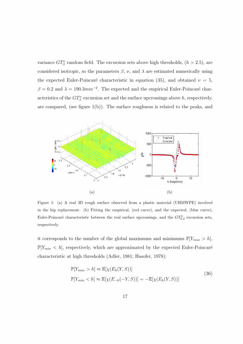
variance GT νβ random field. The excursion sets above high thresholds, (h > 2.5), are

considered isotropic, so the parameters β, ν, and λ are estimated numerically using

the expected Euler-Poincare characteristic in equation (35), and obtained ν = 5,

β = 0.2 and λ = 190.3mm−2. The expected and the empirical Euler-Poincare char-

acteristics of the GT νβ excursion set and the surface upcrossings above h, respectively,

are compared, (see figure 1(b)). The surface roughness is related to the peaks, and

(a) (b)

Figure 1: (a) A real 3D rough surface observed from a plastic material (UHMWPE) involved

in the hip replacement. (b) Fitting the empirical, (red curve), and the expected, (blue curve),

Euler-Poincare characteristic between the real surface upcrossings, and the GT 5

0.2 excursion sets,

respectively.

it corresponds to the number of the global maximums and minimums P[Ymax > h],

P[Ymin < h], respectively, which are approximated by the expected Euler-Poincare

characteristic at high thresholds (Adler, 1981; Hasofer, 1978):

P[Ymax > h] ≈ E[χ(Eh(Y, S))]

P[Ymin < h] ≈ E[χ(E−h(−Y, S))] = −E[χ(Eh(Y, S))](36)

17

Since the expected Euler characteristic above high thresholds, or below low thresh-

olds, counts the number of connected components (isolated peaks or valleys). The

comparison in this example shows that the expected number of the peaks and val-

leys can be estimated accurately from the expected Euler characteristic of the GT νβ

random field which becomes close to the expected Euler-Poincare characteristic of

the student’s t random field at the high thresholds.

5. Conclusion

A random field, denoted by GT νβ , and defined from the linear combination of the

Gaussian random field and student’s t one with ν degrees of freedom scaled by β is

introduced in this paper. The expected Euler-Poincare characteristic and Minkowski

functionals of the GT νβ excursion sets are expressed analytically on a rectangle S of

R2.

An application is reported on a 3D rough surface of a finished UHMWPE plastic

material observed by a non-contact interferometry. Fitting the empirical and the

expected Euler-Poincare charcaterisitc enabled describing the surface roughness. The

future work will focus on studying more flexible random fields including further

significant parameters for modeling the rough surfaces such as the family of the

skewed random fields.

Appendix A. Lemmas for the proof of the Theorem 1

Lemma 3 (Worsley (1994)). Let H ∼ Normald×d(0,M) and let B be a fixed sym-

metric d× d matrix. Then

E[det(B +H)] =

⌊d/2⌋∑

j=0

(−1)j(2j)!

2jdetrd−2j(B) (A.1)

18

Lemma 4 (Cao andWorsley (1999)). Let Q ∼ Wishart(Id, ν), H ∼ Normald×d(0,M)

are independent, and B be a fixed symmetric d× d matrix. Let a, b be fixed scalars.

Then

E[det(B + aQ+ bH)] =

⌊d/2⌋∑

j=0

(−1)j

2jj!b2j

d−2j∑

k=0

ak(

ν

k

)

(2j + k)!detrd−2j−k(B) (A.2)

Adler, R., Taylor, J., july 2011. Topological complexity of smooth random func-

tions: Ecole d’Ete de Probabilites de Saint-Flour XXXIX-2009. Springer Berlin

Heidelberg.

Adler, R. J., June 1981. The Geometry of Random Fields. John Wiley & Sons Inc.

Adler, R. J., Taylor, J., Jun. 2007. Random Fields and Geometry, 1st Edition.

Springer.

Adler, R. J., Taylor, J. E., Worsley, K. J., 2010. Applications of random fields and

geometry: Foundations and case studies.

Alder, R. J., Taylor, J. E., 2003. Random fields and their geometry. Birkhauser,

Boston.

Cao, J., 1997. Excursion sets of random fields with applications to human brain map-

ping. Ph.D. thesis, Departement of Mathematics and Statistics, McGill University,

Quebec, Canada.

Cao, J., Worsley, K., 2001. Applications of random fields in human brain mapping.

Springer lecture notes in statistics 159, 169–182.

Cao, J., Worsley, K. J., 1999. The detection of local shape changes via the geometry

of Hotelling’s t2 fields. The Annals of Statistics 27 (3), 925–942.

19

Hasofer, A. M., Mar. 1978. Upcrossings of random fields. Advances in Applied Prob-

ability 10, 14.

Worsley, K., 1995. Boundary corrections for the expected euler characteristic of ex-

cursion sets of random fields, with an application to astrophysics. Advances in

Applied Probability 27, 943–959.

Worsley, K., 1997. The geometry of random fields. Chance 9 (1), 27–40.

Worsley, K. J., 1994. Local maxima and the expected euler characteristic of excursion

sets of χ2, F and t fields. Advances in Applied Probability 26 (1), 13–42.

20