ON THE ISOPERIMETRIC PROBLEM

FOR RADIAL LOG-CONVEX DENSITIES

A. FIGALLI AND F. MAGGI

Abstract. Given a smooth, radial, uniformly log-convex density eV on Rn, n ≥ 2, we

characterize isoperimetric sets E with respect to weighted perimeterR

∂EeV dHn−1 and

weighted volume m =R

EeV as balls centered at the origin, provided m ∈ [0, m0) for

some (potentially computable) m0 > 0; this affirmatively answers conjecture [RCBM,Conjecture 3.12] for such values of the weighted volume parameter. We also prove thatthe set of weighted volumes such that this characterization holds true is open, thusreducing the proof of the full conjecture to excluding the possibility of bifurcation valuesof the weighted volume parameter. Finally, we show the validity of the conjecture whenV belongs to a C2-neighborhood of c|x|2 (c > 0).

1. Introduction

1.1. Background. Isoperimetric problems in a space with density, a natural generaliza-tion of the classical Gaussian isoperimetric problem [Bo1, SC, Eh, CK, CFMP], havereceived an increasing attention in recent years; see [BBMP, Bo2, CJQW, CMV, DDNT,DHHT, FuMP2, KZ, RCBM, MS, MM, MP]. We refer the reader to [Mo1] for a quickexcursion into the theory of manifolds with density.

As to now, very little is known about the isoperimetric problem with general densities.We consider here a quite basic open question, which can been introduced through anelementary analysis of first and second variation formulae. Precisely, denoting by E anopen set with smooth boundary in R

n, let us consider the isoperimetric-type problem

φV (m) = inf

∫

∂EeV dHn−1 :

∫

EeV = m, E ⊂ R

n

, m > 0 , n ≥ 2 , (1.1)

associated to a positive density eV on Rn, with V : R

n → R radially increasing, that is

V (x) = v(|x|) , for v : (0,∞) → R increasing . (1.2)

The naive intuition that balls centered at the origin should be the only isoperimetric sets(minimizers) in (1.1) is not correct. Indeed, as shown in [DDNT], if n = 2 and eV = |x|p(i.e. v(r) = p log(r), p > 0), then isoperimetric sets are Euclidean disks whose boundariespass through the origin. By computing first and second variations in (1.1), one sees thatevery isoperimetric set E with boundary of class C2 satisfies the stationarity condition

HVE = HE + ∇V · νE = constant on ∂E , (1.3)

and, for every u ∈ C∞c (Rn) with

∫

∂E u eV dHn−1 = 0, the stability inequality

∫

∂E

(

|∇E u|2 − |IIE|2 u2)

eV dHn−1 +

∫

∂E∇2V (νE , νE)u2 eV dHn−1 ≥ 0 (1.4)

holds. (Here, HE denotes the mean curvature of ∂E computed with respect to the outerunit normal νE to E, ∇Eu = ∇u− (∇u ·νE)νE is the tangential gradient of u with respectto ∂E, and IIE is the second fundamental form of ∂E. Our convention is that HE is thetrace of IIE , so that HB = n− 1 if B is the Euclidean unit ball of R

n.)

In particular, balls Br = x ∈ Rn : |x| < r centered at the origin always satisfy the

stationarity condition (1.3), with

HVBr

=n− 1

r+ v′(r) on ∂Br . (1.5)

On the other hand, Br satisfies the stability inequality (1.4) if and only if v′′(r) ≥ 0.Indeed, Br satisfies (1.4) if and only if

ev(r)∫

∂Br

(

|∇Br u|2 −n− 1

r2u2

)

dHn−1 + v′′(r)ev(r)∫

∂Br

u2 dHn−1 ≥ 0 , (1.6)

for every u ∈ C∞c (Rn) such that 0 = ev(r)

∫

∂Bru dHn−1, i.e., with

∫

∂Bru dHn−1 = 0. Then

the stability of balls in the Euclidean isoperimetric problem implies of course that∫

∂Br

(

|∇Br u|2 −n− 1

r2u2

)

dHn−1 ≥ 0 , (1.7)

whenever u ∈ C∞c (Br) and

∫

∂Bru dHn−1 = 0, with equality if and only if u = x · e for

some e ∈ Rn (this corresponds to an infinitesimal translation in the direction e). Taking

this into account, one easily sees that (1.6) holds true on Br if and only if v′′(r) ≥ 0.Hence, in the spirit of [RCBM, Conjecture 3.12], we are naturally led to formulate the

following isoperimetric log-convex density conjecture: for radially increasing log-convexdensities eV on R

n, balls centered at the origin are isoperimetric sets. We shall refer tothe strong form of the conjecture as to the claim that balls centered at the origin arethe unique isoperimetric sets. Note that the assumption of v being increasing is somehownecessary for the validity of this conjecture; for example, as noticed by Morgan [Mo2], ifv(r) = (r− 1)2, then isoperimetric sets with sufficiently small weighted volume have to beuniformly close to a point on S

n−1 (a rigorous justification of this assertion can be derived,for example, using the arguments from sections 5 and 6 below). For the sake of clarity,let us also recall that the existence of isoperimetric sets was proved under the assumptionof the conjecture in [RCBM, Theorem 2.1], and, more generally, whenever v is increasingwith v(r) → +∞ as r → ∞ in [MP, Theorem 3.3].

The validity of the isoperimetric log-convex density conjecture has been supported, upto date, by the following results. For v(r) = c r2, c > 0, the conjecture was proved (beforeits formulation) by Borell [Bo2, Theorem 4.12] through a symmetrization argument. Inthis case, balls centered at the origin are actually the only isoperimetric sets [RCBM,

Theorem 5.2]. This case is somehow special because the densities a ec |x|2, a, c > 0, can

be characterized by the property that the natural notion of Schwartz symmetrizationpreserving the weighted volume Vol(E) decreases the weighted perimeter Per(E), where

Vol(E) =

∫

EeV , Per(E) =

∫

∂EeV dHn−1 ;

see [BBMP, Theorem 3.8]. In [MM], the conjecture has been proved for n = 2 andv(r) = c rp, p ≥ 2, c > 0. A stronger evidence in favor of the conjecture has beenprovided by Kolesnikov and Zhdanov [KZ] through an enlightening argument based onthe divergence theorem. They show that if v is increasing with v′′ ≥ α > 0 on (0,∞), thenthere exists m > 0 such that, for any m > m, balls centered at the origin are the onlyisoperimetric sets with weighted volume m.

1.2. Main results. Before stating our main results, we introduce some useful notation:given m > 0, we denote by r(m) > 0 the radius such that the ball B(m) = Br(m) satisfies

Vol(B(m)) = m ; (1.8)

clearly r(m) is uniquely determined as soon as, for example, v is bounded from below on[0,∞). Moreover, we denote by M(v) the set of those m > 0 such that B(m) is the uniqueisoperimetric set with weighted volume m.

Theorem 1.1. If v ∈ C 2([0,∞); [0,∞)) is an increasing convex function with

inf[0,r]

v′′ > 0 ∀ r > 0 , (1.9)

then the following two assertions hold true:

(i) M(v) is open;(ii) there exists m0 > 0, depending on n and v only, such that (0,m0) ⊂ M(v) (the

value of m0 is potentially computable; see Remark 1.6).

Remark 1.1 (Bifurcation and proof of the complete conjecture). By Theorem 1.1 (resp.by the above mentioned result of Kolesnikov and Zhdanov, if inf(0,∞) v

′′ > 0) we mayreduce the proof of the conjecture to showing that no bifurcation phenomena can occur.More precisely, to prove the conjecture one should show the validity of the followingstatement:

If m > 0 and (0, m) ⊂M(v) (resp. (m,∞) ⊂M(v)), then m ∈M(v).

In other words, we would need to exclude the existence of m > 0 such that both B(m)and E 6= B(m) are isoperimetric sets with weighted volume m, but B(m) is the onlyisoperimetric set with weighted volume m for every m < m (resp. m > m).

Combining Theorem 1.1-(ii), the validity of the conjecture for ec |x|2

(c > 0) [Bo2,RCBM], Kolesnikov-Zhdanov’s Theorem [KZ, Proposition 6.7], and a variant of the ar-gument used in the proof of Theorem 1.1-(i), we shall prove our second main result,namely, the validity of the conjecture on every density eV lying in a sufficiently small

C2-neighborhood of ec |x|2

(see Theorem 1.2 below). An interesting consequence of thisresult is that it shows that the validity of the conjecture for all the weighted volumes is

not a completely exceptional feature related to the special tensorial structure of ec |x|2.

We now state our theorem, introducing the following notation: given w ∈ C0([0,∞))and R > 0, we shall denote by Ω[w](R, ·) the modulus of continuity of w over [0, R], definedas

Ω[w](R,σ) = sup

|w(r) −w(s)| : r, s ∈ [0, R] , |r − s| < σ

, σ > 0 . (1.10)

Observe that, by the local uniform continuity of w, Ω[w](R,σ) → 0 as σ → 0+.

Theorem 1.2. Given n ≥ 2, c > 0, and a function Ω0 : [0,∞) × [0,∞) → [0,∞) withΩ0(R, 0

+) = 0 for every R > 0, there exists a positive constant δ, depending on n, c,and Ω0 only, with the following property: if v ∈ C2([0,∞); [0,∞)) is an increasing convexfunction with

‖v − c r2‖C2([0,∞)) < δ , Ω[v′′](R,σ) ≤ Ω0(R,σ) , ∀R ,σ > 0 , (1.11)

then for every m > 0 the ball B(m) is the unique isoperimetric set in (1.1), that is,M(v) = (0,∞).

Before entering into a closer description of the strategy of proof of Theorem 1.1 we makethe following three remarks.

Remark 1.2 (Densities and Euclidean geometry). Theorem 1.1-(ii) may resemble for cer-tain aspects the main results appearing in our previous paper [FM]. Indeed, in both cases,the starting point of our arguments is exploiting the smallness of the “mass parameter” incombination with the quantitative isoperimetric inequality [FuMP, FiMP, CL] to deducethe L1-proximity of minimizers to balls. However, apart from this similarity, the two prob-lems (and, consequently, the remaining parts of the proofs of our theorems) are completely

different. In particular, what makes the study of this problem extremely delicate is theelusive interaction between geometric quantities such as the mean curvature of E, or theintegrand |∇Eu|2 − |IIE|2u2 in the second variation of the Euclidean perimeter of E (see(1.6) and (1.7)), with the density eV . This point is understood, for example, by noticingthat the stationarity condition (1.3) does not possess any scaling property; or realizingthat the natural notion of Schwarz symmetrization which preserves weighted volume doesnot decrease weighted perimeter, unless v(r) = c r2, c > 0. If these features of the problemmake unlikely its solution by symmetrization techniques, it should also be noted that, atpresent, no characterization results for isoperimetric sets in problems with density havebeen obtained via mass transportation techniques; and this is true even in the case ofthe well-studied Gaussian isoperimetric problem, corresponding to v(r) = −c r2, c > 0.The proof of the characterization result of isoperimetric sets stated in Theorem 1.1-(ii)and Theorem 1.2 is thus quite atypical in its genre: indeed, we will manage to prove aglobal minimality property by combining tools such as the (global) quantitative Euclideanisoperimetric inequality, strict stability properties of candidate minimizers in the problemwith density (obtained in section 2), and improved convergence theorems for sequencesof almost-minimizers of Euclidean perimeter (almost-minimizers are defined in (3.6), andrelated results are discussed in section 3).

Remark 1.3 (Global stability inequalities). As mentioned above, in proving Theorems 1.1and 1.2 we shall establish several local stability results, including in particular a stabilityresult for the ball B(m) with respect to its small C1-perturbations; see Theorem 2.3.Therefore, by using a selection principle in the spirit of [CL, AFM, DM], it may be possibleto deduce from our results global stability inequalities for radial uniformly log-convexdensities eV . We will not investigate further this direction since it does not seem to castfurther light on the isoperimetric log-convex density conjecture, whose understanding isour primary interest here.

Remark 1.4 (Perturbation principle). The perturbation argument behind Theorem 1.2can be suitably adapted to show that, loosely speaking, if v is an increasing, uniformlyconvex function for which the strong conjecture holds at weighted volume m (i.e., m ∈M(v)), then the validity of the conjecture “propagates” to any w close in C2 to v (againwith a uniform bound of the modulus of continuity of w′′), for any value m sufficientlyclose to m. However, since the main explicit example of the validity of the conjecture isobtained by setting v(r) = c r2, we have decided to focus on Theorem 1.2 rather thanstating a more abstract result.

Notation 1. Although the isoperimetric problem (1.1) can be directly formulated onopen sets with smooth boundary, the discussion of the existence and regularity propertiesof isoperimetric sets requires passing through a generalized formulation of the problem.Referring readers to [AFP, Ma] for the technical details (which will play a very marginalrole in our arguments), we shall work here in the framework of the theory of sets offinite perimeter. In particular, given a set of locally finite perimeter E ⊂ R

n, we shalldenote by |E| its Lebesgue measure, by ∂∗E its reduced boundary, by ∂1/2E the set of

points of density one-half of E (recall that ∂∗E ⊂ ∂1/2E and Hn−1(∂1/2E \ ∂∗E) = 0,so one can interchangeably use the two sets when integrating with respect to dHn−1),by P (E;F ) = Hn−1(F ∩ ∂∗E) the distributional perimeter of E relative to the Borel setF ⊂ R

n, and we shall set for brevity

Per(E;F ) =

∫

F∩∂∗EeV dHn−1 ,

for the weighted perimeter of E relative to F as well. By standard approximation theo-rems, the value of φV (m) in (1.1) is unaffected if we minimize among sets of locally finiteperimeter, or among open sets with smooth or Lipschitz or polyhedral boundary.

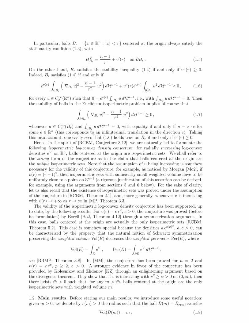
E

r(m)

r(m)(1 + u(ω))ω

Figure 1. A set E defined by u ∈ C1(Sn−1; [−1,∞)) as in (1.14).

1.3. Strategy of proof, Theorem 1.1-(i). We now pass to describe the strategy of proofof Theorem 1.1, starting from statement (i), and introducing the family of isoperimetricsets of weighted volume m, defined as

MV (m) =

E ⊂ Rn : Per(E) = φV (m)

. (1.12)

To prove Theorem 1.1-(i), we first show that for every m2 > m1 > 0 there exists a positiveconstant ε (depending on n, m1, m2, and v only) such that, if γ = inf [0,r(m2)] v

′′ > 0, then

Per(E) ≥ Per(B(m))

1 +γ r(m1)

2

4

∫

−Sn−1

u2

, (1.13)

whenever

E =

t(

1 + u(ω))

ω : ω ∈ Sn−1 , 0 ≤ t < r(m)

, m = Vol(E) ∈ (m1,m2) , (1.14)

for some

u ∈ C1(Sn−1; [−1,∞)) , ‖u‖C1(Sn−1) < ε ;

see Theorem 2.3 in section 2, and Figure 1. This implies in particular that balls centeredat the origin are the unique isoperimetric sets in the restricted competition class of theirsmall C1-perturbations (a result which seems to be new in itself).

We next argue by contradiction; that is, we assume the existence of m > 0 such thatMV (m) = B(m), and of sequences mhh∈N and Ehh∈N with mh → m as h → ∞,Eh ∈ MV (mh), and |Eh∆B(mh)| > 0 for every h ∈ N. Exploiting the minimality of Eh weshow that, up to extracting a subsequence, |Eh∆B(m)| → 0 as h→ ∞. At the same time,the minimality of the Eh in the global isoperimetric problem with density (1.1) impliesin turn their (uniform) local almost-minimality with respect to the Euclidean perimeter:precisely, there exist positive constants C and r0 such that

P (Eh;B(x, r)) ≤ P (F ;B(x, r)) + C rn ,

whenever h ∈ N and Eh∆F ⊂⊂ B(x, r) for some x ∈ Rn and r ≤ r0. In particular,

Ehh∈N is a sequence of uniform almost-minimizers of the perimeter in Rn which converges

in L1 to a smooth limit set, namely, B(m). Then, the regularity theory for almost-minimizers of the perimeter (see section 3) implies the existence of a sequence uhh∈N ⊂C1(Sn−1; [−1,∞)) such that

Eh =

t(

1 + uh(ω))

ω : ω ∈ Sn−1 , 0 ≤ t < r(m)

, limh→∞

‖uh‖C1 = 0 .

(Here, ‖ · ‖C1 = ‖ · ‖C1(Sn−1).) Equivalently, since mh → m there exists uhh∈N ⊂C1(Sn−1; [−1,∞)) such that

Eh =

t(

1 + uh(ω))

ω : ω ∈ Sn−1 , 0 ≤ t < r(mh)

, limh→∞

‖uh‖C1 = 0 .

Hence, for h sufficiently large we can apply (1.13) to conclude

Per(Eh) ≥ Per(B(mh))

1 +γ r(m1)

2

4

∫

−Sn−1

u2h

.

Since none of the Eh’s is a ball, we have uh 6≡ 0 for every h ∈ N; hence Per(Eh) >Per(B(mh)), against Eh ∈ MV (mh).

Remark 1.5. Notice that, having used a compactness argument (together with the as-sumption m ∈M(v)) to deduce that |Eh∆B(m)| → 0 as h→ ∞, we have no informationon the size of the neighborhood of m contained in M(v).

1.4. Strategy of proof, Theorem 1.1-(ii). The strategy of proof is somehow similarto that of statement (i), although quite subtler in several aspects. Consider E ∈ MV (m)for m small. By the quantitative isoperimetric inequality [FiMP], by the above mentionedregularity theory for almost-minimizers of the perimeter, and thanks to some uniformdecay estimates for the diameter of E that we shall prove in section 5, we deduce that, ifm is small enough, then there exist u ∈ C1(Sn−1; [−1,∞)) and a ball B(x0, r) such that

E = x0 +

t(

1 + u(ω))

ω : ω ∈ Sn−1 , 0 ≤ t < r

, limm→0

|x0| + ‖u‖C1 + r = 0 .

Two major difficulties arise at this point. First, even in the case that x0 = 0, we cannotderive a contradiction directly from (1.13), as the constant ε defining the range of appli-cability of (1.13) depends on m, and may be smaller than ‖u‖C1 . Second, it may actuallybe that x0 6= 0, and having no information on the relative sizes of |x0| and r, we do notknow if it is possible to parameterize E over B(m) through C1-small functions (actually,it may even be possible that E does not contain the origin).

The key idea here is that of parameterizing the sets E with respect to the ball B(x0, r)having the same weighted volume and “weighted barycenter”; precisely, we prove theexistence of x0 ∈ R

n, r > 0, and u ∈ C1(Sn−1; [−1,∞)), with

Vol(B(x0, r)) = m,

∫

B(x0,r)x eV (x) dx =

∫

Ex eV (x) dx , (1.15)

and

E = x0 +

t(

1 + u(ω))

ω : ω ∈ Sn−1 , 0 ≤ t < r

, limm→0

|x0| + ‖u‖C1 + r = 0 .

Exploiting the matching of weighted barycenters in (1.15), we are able to take advantageof the Euclidean stability of B(x0, r) to show that if ‖u‖C1 + |x0| < ε0, then

Per(E) ≥ Per(B(x0, r))

1 − C r |x0|∫

−Sn−1

|u| + 1

C

∫

−Sn−1

u2

, (1.16)

where C and ε0 are independent of m; see Theorem 2.1, inequality (2.6), and the proofof Theorem 2.5; notice also the presence of a negative term of order one in (1.16), whichreflects the non-stationarity of balls not centered at the origin in (1.1) in the isoperimetricproblem with radially symmetric density. By a further analysis of the behavior of weightedperimeter on balls, we see that if |x0| ≤ ε1, then

Per(B(x0, r)) ≥ Per(B(m))

1 +|x0|2C

, (1.17)

where ε1 and C are, once again, independent of m; see Theorem 2.4. In conclusion, for msmall enough, combining (1.16) and (1.17) with the elementary inequality

r |x0|∫

−Sn−1

|u| ≤ r

2|x0|2 +

r

2

∫

−Sn−1

|u|2 , (1.18)

we deduce that

Per(E) ≥ Per(B(m))

1 +1

2C

(

|x0|2 +

∫

−Sn−1

u2

)

.

Since E ∈ MV (m), this implies x0 = 0 and u = 0, thus E = B(m), as desired.

Remark 1.6. The value m0 appearing in Theorem 1.1-(ii) is explicitly computable. In-deed, no compactness argument is ever used in the proof, the constant from the quan-titative isoperimetric inequality in [FiMP] is explicit, and all constants appearing in thetheory of almost-minimizers of perimeter from [T2, T1], as well as those appearing in thevarious other steps of the proof outlined above, are (in principle) computable.

1.5. Organization of the paper. In section 2 we gather the various stability estimatesneeded in the proof of Theorem 1.1 and Theorem 1.2, and show in particular that forevery m > 0, B(m) is the unique isoperimetric set among its small C1-perturbations.In section 3 we prove several regularity, symmetry, boundedness, and almost-minimalityproperties of isoperimetric sets which are needed to apply the results proved in section 2to our problem; this is done without needing the convexity of v. In section 4 we proveTheorem 1.1-(i). Then, after showing a quantitative decay estimate on the diameters ofisoperimetric sets in the small weighted volume regime (see section 5), in section 6 wecomplete the proof of Theorem 1.1-(ii). Finally, in section 7, we prove Theorem 1.2.

Acknowledgement. We thank Guido De Philippis for suggesting the inclusion of Theo-rem 1.2, and the anonimous referee for a careful reading and useful comments. The workof AF is supported by NSF Grant DMS-0969962. The work of FM is supported by ERCunder FP7, Starting Grant n. 258685 and Advanced Grant n. 226234. This work wascompleted while FM was visiting the University of Texas at Austin.

2. Some quantitative stability properties of balls centered at the origin

This section is devoted to the proof of various inequalities expressing in a quantitativeway the stability of balls centered at the origin among special families of comparison sets;these inequalities are obtained, of course, under suitable uniform convexity assumptionson v. The key results are: Theorem 2.3, showing in particular that balls centered atthe origin are isoperimetric sets among their C1-small radial perturbations; Theorem 2.4,where we prove a stability (uniform with respect to the weighted volume parameter) ofballs centered at the origin among balls whose centers are sufficiently close to the origin;and Theorem 2.5, where the stability of balls centered at the origin among C1-small radialperturbations of balls whose weighted barycenters are sufficiently close to the origin, isagain proved to be uniform in the small weighted volume parameter.

2.1. Two basic lower-bounds. We start our analysis of local stability properties byproving the two basic lower bounds on the weighted perimeter of a C1-small perturbationof a ball. The first result, Theorem 2.1, is concerned with C1-small perturbations of ballscentered at the origin; the second result, Theorem 2.2, deals with balls not centered at theorigin. Note that, in Theorem 2.1, v is not required to be increasing.

Theorem 2.1. Given n ≥ 2, non-negative constants α, β, and γ, and r2 ≥ r1 > 0, thereexist

ε0 = ε0(n, α, β, γ) ∈(

0,1

2

)

, C0 = C0(n, α, β, γ, r1, r2) <∞ ,

with the following property: If v : (0,∞) → (0,∞) is twice differentiable with

α ≥ |v′| , β ≥ v′′ ≥ γ , on[

(1 − ε0) r1, (1 + ε0) r2]

, (2.1)

and if r > 0, u ∈ C1(Sn−1; [−1,∞)), and

E =

t(

1 + u(ω))

ω : ω ∈ Sn−1 , 0 ≤ t < r

,

are such that

r ∈ [r1, r2] , ‖u‖C1(Sn−1) ≤ ε0 , Vol(E) = Vol(Br) , (2.2)

then

Per(E) ≥ Per(Br)

1 +(

1 − C0‖u‖C1

)γ r2

2

∫

−Sn−1

u2 (2.3)

+

∫

−Sn−1

(

1 − C0‖u‖C1

) |∇u|22

−(

n− 1 + C0‖u‖C1

)u2

2

.

Here ‖u‖C1 = ‖u‖C1(Sn−1), ∇u is the tangential gradient of u on Sn−1, and integration

over Sn−1 is with respect to Hn−1.

Theorem 2.2. Given n ≥ 2, non-negative constants α, β, and γ, and r0 > 0, there exist

ε0 = ε0(n, α, β, γ) ∈(

0,1

2

)

, C0 = C0(n, α, β, γ, r0) <∞ ,

with the following property: If v : (0,∞) → (0,∞) is twice differentiable with

α ≥ v′ ≥ 0 , β ≥ v′′ ≥ γ , on [0, 2 r0] , (2.4)

and if x0 ∈ Rn, r > 0, u ∈ C1(Sn−1; [−1,∞)), and

E = x0 +

t(

1 + u(ω))

ω : ω ∈ Sn−1 , 0 ≤ t < r

,

are such that

|x0| ≤r02, r ≤ r0 , ‖u‖C1(Sn−1) ≤ ε0 , Vol(E) = Vol(B(x0, r)) , (2.5)

then

Per(E) ≥ Per(B(x0, r))

1 − C0 r |x0|∫

−Sn−1

|u| (2.6)

+

∫

−Sn−1

(

1 −C0

(

‖u‖C1 + r0

)) |∇u|22

−(

n− 1 +C0

(

‖u‖C1 + r0

))u2

2

.

Beginning of proof of Theorems 2.1 and 2.2. The first part of the proof of the two theo-rems is common. In the following, we shall denote by C a positive constant dependingon n, α, β, γ, and either r1, r2 or r0 depending on which of the two statements we areconsidering; the value of C may change at each appearance of the constant.

Given x0 ∈ Rn and ω ∈ S

n−1 we introduce the function φω : (0,∞) → (0,∞) defined as

φω(r) =

∫ r

0eV (x0+sω)sn−1 ds , r > 0 . (2.7)

We notice that, for every r > 0,

φ′ω(r) = eV (x0+rω)rn−1 ,

φ′′ω(r) = eV (x0+rω)rn−1(n− 1

r+ ∇V (x0 + rω) · ω

)

,

φ′′′ω (r) = eV (x0+rω)rn−1

(

(n− 1

r+ ∇V (x0 + rω) · ω

)2− n− 1

r2+ ∇2V (x0 + rω)[ω, ω]

)

.

• Step one: We show that, under the assumption of both theorems (and with x0 = 0 inthe case of Theorem 2.1), we have

Per(E) − Per(B(x0, r)) ≥∫

Sn−1

(

rφ′′ω(r)u+r2φ′′ω(r)2

φ′ω(r)

u2

2

)

(2.8)

+(

1 − C ‖u‖C0

) γ r2

2

∫

Sn−1

φ′ω(r)u2

+(

1 − C ‖u‖C1

)

∫

Sn−1

φ′ω(r)|∇u|2

2

−(

n− 1 + C ‖u‖C0

)

∫

Sn−1

φ′ω(r)u2

2.

We start by observing that

∂E = x0 +

r(

1 + u(ω))

ω : ω ∈ Sn−1

.

By applying the area formula on Sn−1 to the Lipschitz function f : S

n−1 → ∂E defined asf(ω) = x0 + r(1 + u(ω))ω, ω ∈ S

n−1, we easily find that

Per(E) =

∫

Sn−1

(

r(1 + u))n−1

eV (x0+r(1+u)ω)

√

1 +|∇u|2

(1 + u)2

=

∫

Sn−1

φ′ω(r(1 + u))

√

1 +|∇u|2

(1 + u)2. (2.9)

By the elementary inequalities

1

(1 + t)2≥ 1 − 2 t , t > −1 ,

√1 + s ≥ 1 +

s

2− s2

8, s ≥ 0 ,

we get√

1 +|∇u|2

(1 + u)2≥ 1 +

(

1 − C ‖u‖C1

) |∇u|22

on Sn−1 . (2.10)

Then, noticing that

∂E ∪ ∂Br ⊂ B(1+ε0) r2 \B(1−ε0) r1 , in the case of Theorem 2.1 , (2.11)

E ∪B(x0, r) ⊂ B2 r0 , in the case of Theorem 2.2 , (2.12)

in both cases we find∣

∣

∣V (x0 + r(1 + u)ω) − V (x0 + rω)

∣

∣

∣≤ αr ‖u‖C0 , ∀ω ∈ S

n−1 ,

and since (1 + t)n−1 ≥ 1 + (n− 1)t > 0 for |t| < 1/(n − 1), we obtain(

r(1 + u))n−1

eV (x0+r(1+u)ω) ≥ rn−1eV (x0+rω)(

1 − C ‖u‖C0

)

on Sn−1 . (2.13)

Thus, combining (2.10) and (2.13) with (2.9) we get

Per(E) ≥∫

Sn−1

φ′ω(r(1 + u)) +(

1 − C ‖u‖C1

)

∫

Sn−1

φ′ω(r)|∇u|2

2. (2.14)

We now notice that, by Taylor’s formula, we can find a function θ : Sn−1 → [0, 1] such

that, if we set u = θ u, then

φ′ω(r(1 + u)) = φ′ω(r) + r φ′′ω(r)u+ r2 φ′′′ω (r(1 + u))u2

2on S

n−1 . (2.15)

Moreover, since

∇2V (x) = v′′(|x|) x

|x| ⊗x

|x| +v′(|x|)|x|

(

Id − x

|x| ⊗x

|x|

)

, ∀x ∈ Rn , (2.16)

we get

∇2V (x0 + r(1 + u)ω)[ω, ω] ≥ γ ,

where in the case of Theorem 2.1 we used that ω is parallel to x0+r(1+ u)ω (since x0 = 0),while in the case of Theorem 2.2 we used that v′(r) ≥ γr (since v′(0) ≥ 0 and v′′ ≥ γ on[0, 2r0]). Thus, by the formula for φ′′′ω and by (2.13) we obtain

r2(1 + u)2 φ′′′ω (r(1 + u)) (2.17)

≥(

1 ± C ‖u‖C0

)

φ′ω(r)

(

n− 1 + ∇V(

x0 + r(1 + u)ω)

· (r(1 + u)ω))2

−(n− 1) + γ r2(1 + u)2

,

where ± is equal to + if the expression inside curly brackets is negative, while ± = − if itis positive. Moreover, in both cases we have

∣

∣

∣∇V

(

x0 + r(1 + u)ω)

· (r(1 + u)ω) −∇V (x0 + rω) · rω∣

∣

∣≤ C ‖u‖C0 ,

which combined with (2.17) gives (with the same convention for ± as before)

r2(1 + u)2 φ′′′ω (r(1 + u))

≥(

1 ± C ‖u‖C0

)

φ′ω(r)

γ r2(1 + u)2 − (n− 1) +

(

n− 1 + ∇V (x0 + rω) · rω)2

− C‖u‖C0

=(

1 ± C ‖u‖C0

)

φ′ω(r)

γ r2(1 + u)2 − (n− 1) + r2φ′′ω(r)2

φ′ω(r)2− C‖u‖C0

.

Multiplying by (1 + u)−2 ≥ (1 − 2 ‖u‖C0) we find

r2 φ′′′ω (r(1 + u)) ≥(

1 ± C ‖u‖C0

)

φ′ω(r)

r2φ′′ω(r)2

φ′ω(r)2+ γ r2 − (n− 1) − C‖u‖C0

≥ r2φ′′ω(r)2

φ′ω(r)+

(

1 ± C ‖u‖C0

)

φ′ω(r)

γ r2 − (n− 1) − C‖u‖C0

,(2.18)

where in the last inequality we used that r2φ′′ω(r)2 ≤ C φ′ω(r)2. We finally combine (2.14),(2.15), and (2.18), to obtain (2.8).

• Step two: We notice that the weighted volume constraint Vol(B(x0, r)) = Vol(E) implies

∫

Sn−1

∫ r

0eV (x0+sω)sn−1 ds =

∫

Sn−1

∫ r(1+u)

0eV (x0+sω)sn−1 ds ,

that is,∫

Sn−1

(

φω(r(1 + u)) − φω(r))

= 0 . (2.19)

By Taylor’s formula, we may define θ : Sn−1 → [0, 1] so that, if u = θu, then

φω(r(1 + u)) = φω(r) + r φ′ω(r)u+ r2 φ′′ω(r)u2

2+ r3 φ′′ω(r(1 + u))

u3

6on S

n−1 .

Inserting this expansion in (2.19) and noticing that, by (2.11) and (2.12), r2|φ′′′ω (r(1+u))| ≤C φ′ω(r), we get the useful estimate

∣

∣

∣

∣

∫

Sn−1

(

rφ′ω(r)u+ r2φ′′ω(r)u2

2

)∣

∣

∣

∣

≤∫

Sn−1

|φ′′′ω (r(1 + u))| (ru)3

6

≤ C ‖u‖C0

∫

Sn−1

rφ′ω(r)u2 , (2.20)

which, combined with r |φ′′ω(r)| ≤ C φ′ω(r), gives in particular∣

∣

∣

∣

∫

Sn−1

φ′ω(r)u

∣

∣

∣

∣

≤ C

∫

Sn−1

φ′ω(r)u2 . (2.21)

We now conclude the proof of Theorem 2.1 and Theorem 2.2 by two separate arguments.

Conclusion of proof of Theorem 2.1. We want to estimate the integral on the first line of(2.8). Since we are assuming that x0 = 0, φ′ω(r) = rn−1ev(r) is constant with respect toω ∈ S

n−1, so (2.20) gives∣

∣

∣

∣

∫

Sn−1

(

rφ′′ω(r)u+r2φ′′ω(r)2

φ′ω(r)

u2

2

)∣

∣

∣

∣

=

∣

∣

∣

∣

φ′′ω(r)

φ′ω(r)

∫

Sn−1

(

rφ′ω(r)u+ r2φ′′ω(r)u2

2

)∣

∣

∣

∣

=

∣

∣

∣

∣

(

n− 1

r+ v′(r)

)∫

Sn−1

(

rφ′ω(r)u+ r2φ′′ω(r)u2

2

)∣

∣

∣

∣

≤ n− 1 + α

rC ‖u‖C0

∫

Sn−1

rφ′ω(r)u2

= C‖u‖C0φ′ω(r)

∫

−Sn−1

u2 .

As φ′ω(r) = Per(Br)/nωn, inserting the above estimate in (2.8) and recalling that γ ≥ 0,we easily get (2.3).

Conclusion of proof of Theorem 2.2. We have to prove (2.6). Let us first show that

Per(E) − Per(B(x0, r)) ≥ −Cr|x0|∫

Sn−1

φ′ω(r)|u| (2.22)

+(

1 − C ‖u‖C1

)

∫

Sn−1

φ′ω(r)|∇u|2

2

−(

n− 1 + C(

‖u‖C0 + r))

∫

Sn−1

φ′ω(r)u2

2.

To this end, we notice that by the formulas for φ′ω and φ′′ω, and by (2.20),∫

Sn−1

(

rφ′′ω(r)u+r2φ′′ω(r)2

φ′ω(r)

u2

2

)

=

∫

Sn−1

φ′′ω(r)

φ′ω(r)

(

rφ′ω(r)u+ r2φ′′ω(r)u2

2

)

=

∫

Sn−1

n− 1

r

(

rφ′ω(r)u+ r2φ′′ω(r)u2

2

)

+

∫

Sn−1

∇V (x0 + rω) · ω(

rφ′ω(r)u+ r2φ′′ω(r)u2

2

)

≥ −C ‖u‖C0

∫

Sn−1

φ′ω(r)u2 + r

∫

Sn−1

∇V (x0 + rω) · ω(

φ′ω(r)u+ rφ′′ω(r)u2

2

)

≥ −C(

‖u‖C0 + r)

∫

Sn−1

φ′ω(r)u2 + r

∫

Sn−1

(

∇V (x0 + rω) · ω)

φ′ω(r)u ,

where in the last step we have used again that r |φ′′ω(r)| ≤ C φ′ω(r) for every r ≤ r0. Wenow notice that, since |∇V (x0 + rω) −∇V (rω)| ≤ β|x0| for every r ≤ r0 and ω ∈ S

n−1,

r

∫

Sn−1

∇V (x0 + rω) · ω φ′ω(r)u (2.23)

= r

∫

Sn−1

∇V (rω) · ω φ′ω(r)u+ r

∫

Sn−1

(

∇V (x0 + rω) −∇V (rω))

· ω φ′ω(r)u

= r v′(r)

∫

Sn−1

φ′ω(r)u+ r

∫

Sn−1

(

∇V (x0 + rω) −∇V (rω))

· ω φ′ω(r)u

≥ −C

r

∫

Sn−1

φ′ω(r)u2 + r|x0|∫

Sn−1

φ′ω(r) |u|

,

where in the last inequality (2.21) was also taken into account. Recalling (2.8) and ne-glecting the term with γ r2, we obtain (2.22). Finally, to conclude the proof of (2.6) itsuffices to observe that

∣

∣

∣φ′ω(r) − rn−1ev(r)

∣

∣

∣≤ α |x0| rn−1 ev(r) ≤ α r0 r

n−1 ev(r) , (2.24)

and∣

∣

∣Per(B(x0, r)) − nωn r

n−1eV (x0)∣

∣

∣≤ α |x0|Per(B(x0, r)) ≤ α r0 Per(B(x0, r)) . (2.25)

In particular∫

Sn−1

φ′ω(r)|u| ≤ nωnrn−1ev(r)(1 + C r0)

∫

−Sn−1

|u| ≤ C Per(B(x0, r))

∫

−Sn−1

|u| ,

as well as,∫

Sn−1

φ′ω(r)|∇u|2

2≥ Per(B(x0, r))(1 − α r0)

2

∫

−Sn−1

|∇u|22

,

∫

Sn−1

φ′ω(r)u2

2≤ Per(B(x0, r))(1 + αr0)

2

∫

−Sn−1

u2

2.

By plugging these last three inequalities into (2.22), we obtain (2.6).

2.2. Stability of balls centered at the origin. Following a technique developed byFuglede to study the stability of the Euclidean isoperimetric inequality on nearly sphericaldomains, see [Fu1, Fu2], we now combine the lower bound (2.3) in Theorem 2.1 withan expansion in spherical harmonics to prove the minimality of balls centered at theorigin with respect to C1-small radial perturbations. Let us recall that, given m > 0,we denote by B(m) = Br(m) the ball of radius r(m) > 0 centered at the origin suchthat Vol(B(m)) = Vol(Br(m)) = m. Notice that in this theorem v is not required to beincreasing, but just locally uniformly convex.

Theorem 2.3. Given n ≥ 2, positive constants α, β, and γ, and m2 ≥ m1 > 0, thereexists

ε1 = ε1(n, α, β, γ,m1,m2) ∈(

0,1

2

)

,

with the following property: If v : [0,∞) → [0,∞) is twice differentiable with

α ≥ |v′| , β ≥ v′′ ≥ γ , on[

(1 − ε1) r(m1), (1 + ε1) r(m2)]

,

and if u ∈ C1(Sn−1), m ∈ [m1,m2], and

E =

t(

1 + u(ω))

ω : ω ∈ Sn−1 , 0 ≤ t < r(m)

are such that

‖u‖C1 ≤ ε1 min

r(m1)2, 1

, Vol(E) = m,

then

Per(E) ≥ Per(B(m))

1 +γ r(m1)

2

4

∫

−Sn−1

u2

. (2.26)

In particular, if E is an isoperimetric set then E = B(m).

Remark 2.1. As a consequence of Theorem 2.3, B(m) is the unique isoperimetric setamong its C1-small perturbations. In fact, it is a strictly stable isoperimetric set in thisrestricted competition class, and (2.26) quantitatively shows that, due to the uniformconvexity of v, this minimality property becomes increasingly stronger as we increase theweighted volume parameter. At the same time we should notice that this theorem is notparticularly useful in the small weighted volume regime: indeed, both the lower bound onPer(E) − Per(B(m)) in (2.26) and the range of applicability of (2.26) in terms of the sizeof ‖u‖C1(Sn−1) degenerate as m1 → 0+.

Proof of Theorem 2.3. Let ε0 be the constant determined by Theorem 2.1 in correspon-dence with n, α, β, γ, r1 = r(m1), and r2 = r(m2), and let C denote a generic constantdepending on n, α, β, γ, r1, and r2 only. Applying (2.3) with r = r(m) (note thatr ∈ (r1, r2) since v ≥ 0 and thus Vol(Br) is strictly increasing as a function of r), we have

Per(E) ≥ Per(Br)

1 +(

1 − C ‖u‖C1

)γ r2

2

∫

−Sn−1

u2

(2.27)

+Per(Br)

∫

−Sn−1

(

1 − C ‖u‖C1

) |∇u|22

−(

n− 1 + C ‖u‖C1

)u2

2,

provided ‖u‖C1 ≤ ε0. Our goal is now to estimate from below that term in the secondline. To this end, let us consider the orthonormal basis of L2(Sn−1) given by the sphericalharmonics Yj,k : 1 ≤ k ≤ nj∞j=0, that is

∫

−Sn−1

Yj,kYℓ,q = δj,ℓδk,q,

∫

−Sn−1

|∇Yj,k|2 = λj = j(n − 2 + j) ,

and denote the coefficients of u with respect to this basis as

cj,k =

∫

−Sn−1

Yj,k u .

Since λ1 = n− 1 and λj ≥ 2n for every j ≥ 2, we find(

1 − C‖u‖C1

)

∫

−Sn−1

|∇u|2 −(

n− 1 + C‖u‖C1

)

∫

−Sn−1

u2

=(

1 − C‖u‖C1

)

∑

j,k

λjc2j,k −

(

n− 1 + C‖u‖C1

)

∑

j,k

c2j,k

≥(

n+ 1 − C ‖u‖C1

)

∑

j≥2

∑

k

c2j,k − C ‖u‖C1

n1∑

k=1

c21,k − n c20

≥ −C ‖u‖C1

n1∑

k=1

c21,k − n c20 . (2.28)

As x0 = 0, φ′ω(r) = rn−1ev(r) is constant on Sn−1; hence, by (2.21) we find that

∣

∣

∣

∣

∫

Sn−1

u

∣

∣

∣

∣

≤ C

∫

Sn−1

u2 ≤ C ‖u‖C0

∫

Sn−1

|u| ,

so that, by Holder inequality and recalling that Y0 = 1,

c20 =

∣

∣

∣

∣

∫

−Sn−1

u

∣

∣

∣

∣

2

≤ C ‖u‖2C0

∫

−Sn−1

u2 . (2.29)

Since∫

−Sn−1

u2 =∑

j≥0

∑

k

c2j,k ≥n1∑

k=1

c21,k , (2.30)

combining (2.27), (2.28), (2.29), and (2.30) we conclude

Per(E) ≥ Per(Br)

1 +

(

(

1 − C ‖u‖C1

)γ r2

2− C ‖u‖C1

)∫

−Sn−1

u2

≥ Per(Br)

1 +

(

(

1 − C ‖u‖C1

)γ r(m1)2

2− C ‖u‖C1

)∫

−Sn−1

u2

,

where in the last inequality we have use the fact that r = r(m) ≥ r(m1). Then (2.26)follows immediately provided ‖u‖C1 ≤ ε1 minr(m1)

2, 1 for a suitable ε1 ≤ ε0.

2.3. Perturbation of balls not centered at the origin. We shall now explain how toexploit (2.6) under the assumption that B(x0, r) and E not only have the same weightedvolume, but also share the same weighted barycenter; as noticed in the introduction, thisanalysis will be needed to tackle the conjecture in the small weighted volume regime,although we shall not use a small weighted volume assumption in the following discussion.

We start by showing that balls centered at the origin are the unique isoperimetric setsamong balls centered sufficiently close to the origin, uniformly with respect to the weightedvolume parameter; see Theorem 2.4. In Theorem 2.5, starting from (2.6) in Theorem2.1, we extend this uniform stability property among all C1-small radial perturbations ofballs having weighted barycenter sufficiently close to the origin. We recall the notationΩ[w](R, ·) for the modulus of continuity of a continuous function w over the interval [0, R];see (1.10).

Theorem 2.4. Given n ≥ 2, positive constants α, β, γ, and m0, and v ∈ C2([0,∞); [0,∞))a convex increasing function with

α ≥ v′ ≥ 0 , β ≥ v′′ ≥ γ , on [0, 2 r(m0)] ,

there exists

t0 = t0

(

n, α, β,Ω[v′′](2 r(m0), ·))

> 0 ,

with the following property: if |x0| ≤ t0 and r > 0 is such that Vol(B(x0, r)) = m ≤ m0,then

Per(B(x0, r)) ≥ Per(B(m))

1 +γ

8n|x0|2

. (2.31)

Proof. Fix m < m0, and denote by s(t) the radius of the ball centered at te1 satisfying

m = Vol(B(t e1, s(t))) =

∫

Bs(t)

eV (x+te1) dx , t > 0 ;

notice that s ∈ C2([0,∞); [0, r(m0)]) and s(0) = r(m). Correspondingly, let us considerthe function f ∈ C2([0,∞); (0,∞)) defined as

f(t) = Per(B(te1, s(t))) =

∫

Sn−1

s(t)n−1 eV (s(t)ω+t e1) dHn−1(ω) , t > 0 .

We claim that

f ′′(0) ≥ γ

nf(0) , (2.32)

|f ′| ≤ C f , on [0, r(m0)] , (2.33)

f ′′

f∈ C0([0, r(m0)]) , (2.34)

where C depends only on n, α, and β, and where the modulus of continuity of f ′′/f over[0, r(m0)] depends only on the moduli of continuity of v, v′, and v′′ over [0, 2r(m0)]. Beforeproving these claims, let us explain how they lead to conclude the proof of the theorem.

By (2.33) the function t 7→ f(t) eC t is increasing over [0, r(m0)], hence there existst0 < r(m0) such that

f(t) ≥ f(0)

2, ∀ t ∈ [0, t0] ; (2.35)

moreover, by (2.34) and by (2.32), up to decrease the value of t0,

f ′′(t)

f(t)≥ γ

2n∀ t ∈ [0, t0] . (2.36)

We may thus combine (2.35) and (2.36) to find that

f ′′(t) ≥ γ

4nf(0) , ∀ t ∈ [0, t0] ,

which by Taylor’s formula gives

f(t) ≥ f(0)(

1 +γ

8nt2

)

, ∀ t ∈ [0, t0] . (2.37)

If now x0 ∈ Rn with |x0| < t0, and r > 0 is such that Vol(B(x0, r)) = m, then r = s(t)

and Per(B(x0, r)) = Per(B(t e1, s(t))) for t = |x0| so that (2.37) gives exactly (2.31). Weare thus left to prove the validity of (2.32), (2.33), and (2.34).

To this end, we start differentiating the identity defining s(t) to find that

s′(t) = − 1

f(t)

∫

Bs(t)

eV (x+te1)∂1V (x+ te1) dx , (2.38)

s′′(t) = − 1

f(t)

∫

Bs(t)

eV (x+te1)(

∂1V (x+ te1)2 + ∂11V (x+ te1)

)

dx

−s′(t)

f(t)

∫

∂Bs(t)

eV (ω+te1)∂1V (ω + te1) dHn−1(ω)

+f ′(t)

f(t)2

∫

Bs(t)

eV (x+te1)∂1V (x+ te1) dx.

Observing that

eV (x+te1)∂1V (x+ te1) = ∂1

(

eV (x+te1))

,

eV (x+te1)(

∂1V (x+ te1)2 + ∂11V (x+ te1)

)

= ∂1

(

eV (x+te1)∂1V (x+ te1))

,

and setting ν1 = νBs(t)· e1, we can rewrite s′′(t) as

s′′(t) = − 1

f(t)

∫

∂Bs(t)

eV (ω+te1)∂1V (ω + te1)ν1(x) dHn−1(ω) (2.39)

−s′(t)

f(t)

∫

∂Bs(t)

eV (ω+te1)∂1V (ω + te1) dHn−1(ω)

+f ′(t)

f(t)2

∫

∂Bs(t)

eV (ω+te1)ν1(ω) dHn−1(ω) .

We finally compute

f ′(t) = (n− 1)s′(t)

s(t)f(t) +

∫

Sn−1

s(t)n−1eV (s(t)ω+te1)(

s′(t)ω · ∇V + ∂1V)

dHn−1(ω) ,

(2.40)

f ′′(t) = (n− 1)

(

s′′(t)

s(t)− s′(t)2

s(t)2

)

f(t) + (n− 1)s′(t)

s(t)f ′(t)

+(n− 1)s′(t)

s(t)

∫

Sn−1

s(t)n−1eV (s(t)ω+te1)(

s′(t)ω · ∇V + ∂1V)

dHn−1(ω)

+

∫

Sn−1

s(t)n−1eV (s(t)ω+te1)(

s′(t)ω · ∇V + ∂1V)2dHn−1(ω)

+s′′(t)

∫

Sn−1

s(t)n−1eV (s(t)ω+te1)(

ω · ∇V)

dHn−1(ω)

+

∫

Sn−1

s(t)n−1eV (s(t)ω+te1)∇2V(

s′(t)ω + e1, s′(t)x+ e1

)

dHn−1(ω) ,

where ∂1V , ∇V , and ∇2V are all evaluated at te1 + s(t)x. We now notice that, by (2.38),(2.40), and by symmetry,

s′(0) =1

f(0)

∫

Bs(0)

ev(|x|)v′(|x|)|x| (x · e1) dx = 0 ,

f ′(0) = s(0)n−1ev(s(0))v′(s(0))

s(0)

∫

Sn−1

(ω · e1) dHn−1(ω) = 0 .

In particular, since

1 =

∫

−Sn−1

|ω|2dHn−1(ω) = n

∫

−Sn−1

(ω · e1)2 dHn−1(ω) (2.41)

using (2.39) we may compute s′′(0) as

s′′(0) = −v′(s(0))∫

−Sn−1

(e1 · ω)2 dHn−1(ω) = −v′(s(0))

n.

Finally, taking into account that f(0) = nωns(0)n−1ev(s(0)), we find

f ′′(0)

f(0)= (n− 1)

s′′(0)

s(0)+ v′(s(0))2

∫

−Sn−1

(ω · e1)2 dHn−1(ω)

+s′′(0) v′(s(0)) +

∫

−Sn−1

∂211V (s(0)ω) dHn−1(ω)

= −(n− 1)

n

v′(s(0))

s(0)+

∫

−Sn−1

∂211V (s(0)ω) dHn−1(ω) .

Recalling (2.16), we find that

∂11V (r ω) = v′′(r) (ω · e1)2 +v′(r)

r

(

1 − (ω · e1)2)

, ∀ r > 0 , ω ∈ Sn−1 ,

and thus, again by (2.41) and recalling that v is uniformly convex on [0, r(m0)],

f ′′(0)

f(0)= −(n− 1)

n

v′(s(0))

s(0)+v′′(s(0))

n+v′(s(0))

s(0)

(

1 − 1

n

)

=v′′(s(0))

n. (2.42)

This proves the validity of (2.32), while (2.33) and (2.34) follow easily by examining theformulas for f , f ′, f ′′, s′, and s′′ derived above.

We now extend the uniform stability property of Theorem 2.4 to C1-small radial per-turbations of balls with small weighted barycenter.

Theorem 2.5. Given n ≥ 2, positive constants α, β, γ, and m0, v ∈ C2([0,∞); [0,∞)) aconvex increasing function with

α ≥ v′ ≥ 0 , β ≥ v′′ ≥ γ , on [0, 2 r(m0)] ,

there exist

ε2 = ε2(n, α, β, γ,m0) > 0 , C1 = C1(n, α, β, γ,m0) <∞ ,

r1 = r1

(

n, α, β, γ,m0,Ω[v′′](2 r(m0), ·))

> 0 ,

with the following property: if x0 ∈ Rn, r > 0, u ∈ C1(Sn−1; [−1,∞)) and

E = x0 +

t (1 + u(ω))ω : ω ∈ Sn−1 , 0 ≤ t < r

,

are such that|x0| ≤ r1 , r ≤ r1 , ‖u‖C1(Sn−1) ≤ ε2 ,

and satisfy the weighted volume and weighted barycenter constraints

Vol(E) = Vol(B(x0, r)) = m ≤ m0 ,

∫

B(x0,r)x eV (x) dx =

∫

Ex eV (x)dx , (2.43)

then

Per(E) ≥ Per(B(m))

1 +1

C1

(

|x0|2 +

∫

−Sn−1

u2

)

. (2.44)

In particular, if E is an isoperimetric set, then E = B(m).

Proof. Let ε0 be the positive constant defined by Theorem 2.1 in correspondence withn, α, β, γ, and r0 = r(m0), and let t0 be the positive constant defined by Theorem 2.4starting from n, α, β, and the moduli of continuity of v′′ on [0, 2 r(m0)]. We denote by Ca generic constant depending on n, α, β, γ, and m0 only. Provided

|x0| ≤r02, r ≤ minr0, t0 , ‖u‖C1 ≤ ε0 ,

as we can certainly assume by requiring r1 ≤ mint0, r0/2 and ε2 ≤ ε0, by (2.6) inTheorem 2.1 we have that

Per(E) ≥ Per(B(x0, r))

1 − C r |x0|∫

−Sn−1

|u| (2.45)

+

∫

−Sn−1

(

1 − C(

‖u‖C1 + r1

)) |∇u|22

−(

n− 1 + C(

‖u‖C1 + r1

))u2

2

,

while (2.31) in Theorem 2.4 gives

Per(B(x0, r)) ≥ Per(B(m))

1 +γ

8n|x0|2

. (2.46)

Expanding u in spherical harmonics as in the proof of Theorem 2.3, we see that∫

−Sn−1

(

1 − C(

‖u‖C1 + r1

)) |∇u|22

−(

n− 1 + C(

‖u‖C1 + r1

))u2

2(2.47)

≥(

n+ 1 − C(

‖u‖C1 + r1

))

∑

j≥2

∑

k

c2j,k − C(

‖u‖C1 + r1

)

n1∑

k=1

c21,k − n c20 ,

where

c0 =

∫

−Sn−1

u , c1,k =

∫

−Sn−1

(ω · ek)u , k = 1, . . . , n , (n1 = n) .

By (2.21), (2.24), and (2.25), we find∣

∣

∣

∣

∫

−Sn−1

u

∣

∣

∣

∣

≤ C

(

|x0|∫

−Sn−1

|u| +∫

−Sn−1

u2

)

, (2.48)

therefore

c20 =

(∫

−Sn−1

u

)2

≤ C(

|x0|2 + ‖u‖2C0

)

∫

−Sn−1

u2 . (2.49)

By the barycenter constraint (2.43) we now see that, if we define

ψω(t) =

∫ t

0sn eV (x0+sω) ds , t > 0 ,

then

0 =

∫

Ex eV (x)dx−

∫

B(x0,r)x eV (x) dx =

∫

Sn−1

ω(

ψω(r(1 + u)) − ψω(r))

. (2.50)

Thus, recalling the definition (2.24) of φω, we have

ψ′ω(t) = tn eV (x0+t ω) = t φ′ω(t) ,

ψ′′ω(t) = tn eV (x0+t ω)

(n

t+ ∇V (x0 + t ω) · ω

)

.

By Taylor’s formula, this implies that

ψω(r(1 + u)) − ψω(r) = rφ′ω(r) ru+ ψ′′ω

(

r(1 + θu))(ru)2

2

for a suitable function θ : Sn−1 → [0, 1], and since |ψ′′

ω(r(1 + θu))| ≤ C φ′ω(r), (2.50) gives

r2∣

∣

∣

∣

∫

Sn−1

ω uφ′ω(r)

∣

∣

∣

∣

=

∣

∣

∣

∣

∫

Sn−1

ω ψ′′ω

(

r(1 + θu))(ru)2

2

∣

∣

∣

∣

≤ C r2∫

Sn−1

φ′ω(r)u2 .(2.51)

Again by (2.24), and since φ′ω(r) ≤ C rn−1 ev(r), we deduce from (2.51) that

∣

∣

∣

∣

∫

−Sn−1

ω u

∣

∣

∣

∣

≤ C(

|x0|∫

−Sn−1

|u| +∫

−Sn−1

u2)

≤ C(

‖u‖C0 + r1)

(∫

−Sn−1

u2

)1/2

,

Therefore,n

∑

k=1

c21,k =

∣

∣

∣

∣

∫

−Sn−1

ω u

∣

∣

∣

∣

2

≤ C(

‖u‖C0 + r1)2

∫

−Sn−1

u2 . (2.52)

By (2.49) and (2.52), since∫

−Sn−1

u2 =∑

j≥0

∑

k

c2j,k ,

we see that∑

j≥2

∑

k

c2j,k >1

2

∫

−Sn−1

u2 ,

so that (2.45) and (2.47) give

Per(E) ≥ Per(B(x0, r))

1 +n

2

∫

−Sn−1

u2 − C r |x0|∫

−Sn−1

|u|

. (2.53)

Finally, using (2.46) we conclude that

Per(E) ≥ Per(B(m))

1 +1

C

(

|x0|2 +

∫

−Sn−1

u2

)

− C r|x0|∫

−Sn−1

|u|

,

and (2.44) follows by Young’s inequality (see (1.18)) provided r1 is small enough.

3. Some properties of isoperimetric sets

In this section we gather several properties of isoperimetric sets which shall be used inproving Theorems 1.1 and 1.2. We begin with a lemma which was first obtained by Morganand Pratelli in [MP, Proof of Theorem 3.3] while proving the existence of isoperimetricsets when v is increasing and diverges as r → ∞. As we shall use their argument to provevarious uniform estimates, we include it in the following lemma for the sake of clarity.Given n ≥ 2, let κ(n) denote the isoperimetric constant on the sphere S

n−1, that is,

κ(n) = inf

Hn−2(∂G)

Hn−1(G)(n−2)/(n−1): G ⊂ S

n−1 , ∂G smooth ,Hn−1(G) ≤ Hn−1(Sn−1)

2

.

(3.1)We also recall that P (E) denotes the Euclidean distributional perimeter of a Borel set E.

Lemma 3.1. Given n ≥ 2 and M > 0 set

R0(n,M) :=

(

2M

nωn

)1/(n−1)

. (3.2)

If v : (0,∞) → (0,∞) is increasing and P (E) ≤M , then

Per(E;Bcr) ≥ κ(n)(n−1)/n ev(r)/n Vol(E \Br)(n−1)/n , ∀ r ≥ R0 . (3.3)

Remark 3.1. If v is convex, then the following “Euclidean” lower bound was proved byKolesnikov and Zhdanov [KZ, Proposition 6.5]:

Per(E) ≥ nω1/nn ev(0)/nVol(E)(n−1)/n , ∀E ⊂ R

n .

Proof of Lemma 3.1. Since perimeter is decreased by taking intersections with convex sets[Ma, Exercise 15.14], we have P (E) ≥ P (E ∩ Bs), where, for a.e. s > 0, P (E ∩ Bs) =P (E;Bs) + Hn−1(E ∩ ∂Bs), see [Ma, Lemma 15.1]; hence,

P (E;Bcs) ≥ Hn−1(E ∩ ∂Bs) , for a.e. s > 0 .

Since v is increasing and P (E;Bcs) is decreasing in s, this implies

Per(E;Bcr) ≥ ev(r) ess sup

s>rP (E;Bc

s) ≥ ev(r) ess sups>r

Hn−1(E ∩ ∂Bs) (3.4)

for every r > 0. Moreover, we also get

Hn−1(E ∩ ∂Bs)sn−1

≤ P (E;Bcs)

sn−1≤ M

sn−1for a.e. s > 0 .

SinceM

sn−1≤ nωn

2, ∀ s ≥ R0 ,

by a scaling and approximation argument and by definition of κ(n), we get

Hn−2(∂∗E ∩ ∂Bs) ≥ κ(n)Hn−1(E ∩ ∂Bs)(n−2)/(n−1) , ∀ s ≥ R0 .

Let us now recall that, being ∂∗E a locally Hn−1-rectifiable set in Rn, then the coarea

formula [Ma, Theorem 18.8]∫

∂∗Eg

√

|∇u|2 − (νE · ∇u)2 dHn−1 =

∫

R

dt

∫

∂∗E∩u=tg dHn−2

holds for every Lipschitz function u : Rn → R and Borel function g : R

n → [0,∞]. Inparticular, if we set

u(x) = |x| , g(x) = 1∂∗E\Br(x) eV (x) ,

then the coarea formula gives

Per(E;Bcr) ≥

∫

∂∗E\Br

eV (x)√

1 − (νE(x) · x/|x|)2 dHn−1

=

∫ ∞

rev(s)Hn−2(∂∗E ∩ ∂Bs) ds

≥ κ(n)

∫ ∞

rev(s)Hn−1(E ∩ ∂Bs)(n−2)/(n−1) ds

≥ κ(n)∫ ∞r ev(s)Hn−1(E ∩ ∂Bs) dr

esssups>rHn−1(E ∩ ∂Bs)1/(n−1)

=κ(n)Vol(E \Br)

esssups>rHn−1(E ∩ ∂Bs)1/(n−1),

which combined with (3.4) immediately gives (3.3).

An immediate corollary is the following theorem, see [MP, Theorem 3.3].

Theorem 3.1 (Existence theorem). If v : [0,∞) → R is increasing, with

limr→∞

v(r) = +∞ , (3.5)

and Ehh∈N is a sequence of sets with uniformly bounded weighted perimeters and vol-umes, then there exists E ⊂ R

n such that, up to extracting a subsequence, Vol(Eh∆E) → 0as h → ∞. In particular MV (m) (the family of isoperimetric sets with weighted volumem, see (1.12)) is non-empty for every m > 0.

Proof. This follows easily from standard lower semicontinuity and compactness theoremsfor sets of finite perimeter [Ma, Chapter 12] thanks to condition (3.3), which preventsminimizing sequences to concentrate mass at infinity; see [MP, Section 3] for more details.

We now gather the basic symmetry and regularity properties of isoperimetric sets.Concerning regularity properties, the key notion here is that of almost-minimality forthe perimeter, introduced by Almgren in [Al] in a much more general context, and laterrephrased and developed by Bombieri [B] and Tamanini [T1, T2] on integer rectifiable cur-rents and sets of finite perimeter respectively. For the purposes of this paper, it suffices tosay that a set of locally finite perimeter E in R

n is an almost-minimizer for the perimeterif there exist positive constants C and r0 such that

P (E;B(x, r)) ≤ P (F ;B(x, r)) + C rn , (3.6)

whenever E∆F ⊂⊂ B(x, r) and r < r0. Referring to [T1, Chapter 1] or to [Ma, Chapter21] for some heuristics, motivations, variants, and generalizations of this definition, we

limit ourselves here to recall that if E satisfies (3.6), then ∂∗E is a C1,1/2-hypersurface,and that, after modifying E on a set of Lebesgue measure zero, the singular set ∂E \ ∂∗Ehas Hausdorff dimension at most n − 8; see [T1, 1.9] or [T2, Theorem 1]. Moreover, ifEhh∈N is a sequence of almost-minimizers with uniform constants C and r0, and Ehlocally converges to E in L1, then E is an almost-minimizer. In addition, given x ∈ ∂∗Ethere exists rx > 0 and hx ∈ N such that B(x, rx) ∩ ∂E and B(x, rx) ∩ ∂Eh (h ≥ hx) aregraphs (over a same (n− 1)-dimensional disk) of functions u and uh (h ≥ hx) respectively,with uh → u in C1,1/2.

Theorem 3.2 (Qualitative properties of isoperimetric sets). If v : [0,∞) → [0,∞) issmooth (resp. analytic) and E ∈ MV (m), m > 0, then (up to a modification of E on a

set of measure zero) E is a bounded set and ∂E is a C1,1/2 hypersurface on Rn. Moreover

∂E \ 0 is smooth (resp. analytic), and there exists a line ℓ passing through the originsuch that E is symmetric by rotation with respect to ℓ, with

HVE = HE + ∇V · νE = constant , on ∂E \ 0. (3.7)

Moreover, if v is increasing, then the isoperimetric function φV defined in (1.1) is strictlyincreasing and continuous on (0,∞), and

φ′V (m+) ≤ HVE ≤ φ′V (m−) , ∀E ∈ MV (m) .

Remark 3.2. Notice that in the above result eV does not need to be smooth at 0 (for

instance, if v(r) = r then eV = e|x|). However, if eV is smooth also at the origin, then theproof below actually shows that ∂E is globally smooth (analytic).

Proof of Theorem 3.2. Some of the arguments in this proof are well known to specialists,but we include some details and references for convenience of the reader.

• Step one: First of all we observe that, up to change E ∈ MV (m) on a set of Lebesguemeasure zero, we can ensure that the reduced boundary ∂∗E is dense in the topologicalboundary ∂E of E, with the characterization

∂E =

x ∈ Rn : 0 < |E ∩B(x, r)| < ωn r

n , ∀ r > 0

;

see for instance [Ma, Proposition 12.19]. The boundedness of E follows by a rather stan-dard argument based on the isoperimetric inequality, that in the present context is detailedin [RCBM, Theorem 2.1]. As explained above, to show that ∂∗E is a C1,1/2-hypersurfacewhich is relatively open (and dense) inside ∂E, and that the singular set Σ(E) = ∂E \∂∗Ehas Hausdorff dimension at most n − 8, it suffices to show that E is an almost-perimeterminimizer in R

n; notice that, once C1,1/2-regularity is proved, and since V is smooth out-side the origin, then the (distributional form of the) Euler-Lagrange equation (3.7) consid-ered in local coordinates will imply by standard elliptic regularity theory that ∂∗E \0 isa smooth hypersurface in R

n - in fact, analytic, if v is so - see [Ma, Chapter 27] for moredetails. Since E ⊂ BR−1 for some large radius R > 0, it suffices to prove that there existpositive constants C and s0 ∈ (0, 1) (possibly depending on E, R, and v) such that

P (E;B(x, s)) ≤ P (F ;B(x, s)) + C sn (3.8)

whenever E∆F ⊂⊂ B(x, s) ⊂ BR and s < s0 (indeed, if B(x, s) 6⊂ BR then E ∩B(x, s) ⊂BR−1 ∩B(x, s) = ∅, so (3.8) is trivially satisfied).

Since eV is uniformly positive and locally Lipschitz on Rn, by a minor modification

of [Ma, Lemma 17.21] we find two balls B(x1, r) and B(x2, r) lying at mutually positivedistance, and two positive constants C0 and σ0 (depending on E, R, and v only), suchthat for every σ ∈ (−σ0, σ0) there exist two sets of finite perimeter F1 and F2, with

E∆Fk ⊂⊂ B(xk, r) , Vol(Fk) = Vol(E) + σ ,∣

∣

∣Per(E;B(x, r)) − Per(Fk;B(x, r))

∣

∣

∣≤ C0 |σ| , k = 1, 2 .

(These sets are constructed using the flow of two smooth vector fields, respectively sup-ported inside B(x1, r) and B(x2, r), which are almost pointing in the direction of thenormal, see the proof of [Ma, Lemma 17.21] for more details.)

Let us now fix any ball B(x, s) ⊂ BR with s < s0, where s0 is chosen sufficiently smallso that ωn s

n0 < σ0 and

either |x− x1| > s0 + r or |x− x2| > s0 + r .

If F is any set of finite perimeter with E∆F ⊂⊂ B(x, s), and assuming without loss ofgenerality that B(x, s) ∩ B(x1, r) = ∅, we define σ := Vol(E) − Vol(F ) and consider the

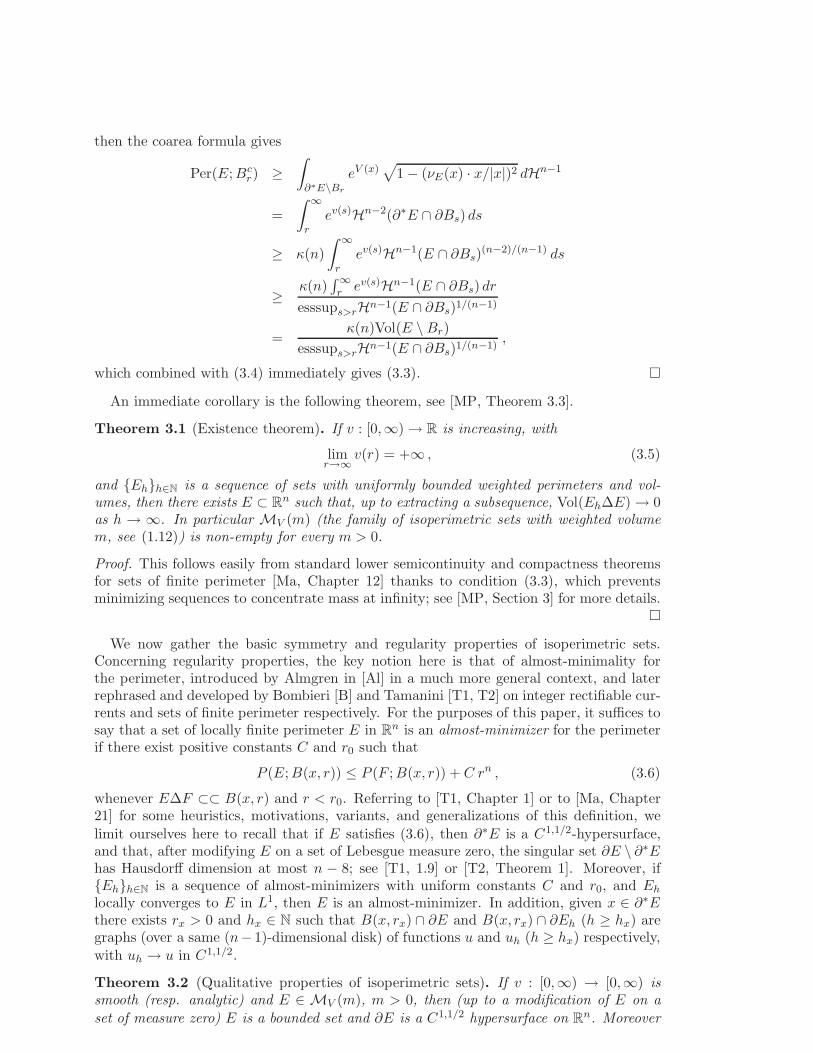
E

0

ℓ0

Figure 2. Symmetrization by spherical caps with respect to an half-line ℓ0 pre-

serves weighted volume and decreases weighted perimeter. In the picture, a set

which is left invariant by spherical symmetrization (note that the orthogonal sec-

tions of E with respect to ℓ0 need not to be (n− 1)-dimensional balls).

set F1 given by the construction described above. Then it is immediate to check that theset

G =(

F ∩B(x, s))

∪(

F1 ∩B(x1, r))

∪(

E ∩(

B(x, s) ∪B(x1, r))c)

satisfies Vol(G) = Vol(E), so by minimality Per(E) ≤ Per(G). We thus find

Per(E;B(x, s) ∪B(x1, r)) ≤ Per(F ;B(x, s)) + Per(F1;B(x1, r)) ,

which in turn implies

Per(E;B(x, s)) ≤ Per(F ;B(x, s)) + C0 |Vol(E) − Vol(F )|≤ Per(F ;B(x, s)) + C0 e

v(R) ωn sn .

Since eV is a locally Lipschitz function on Rn, there exists a constant C1, depending only

on R and v, such that

Per(E;B(x, s)) ≥ eV (x)(1 − C1 s)P (E;B(x, s)) ,

Per(F ;B(x, s)) ≤ eV (x) (1 + C1 s)P (F ;B(x, s)) .

In conclusion, for a constant C2 depending on E, v, and R only, we conclude that

P (E;B(x, s)) ≤ (1 + C2 s)P (F ;B(x, s)) + C2 sn , (3.9)

whenever E∆F ⊂⊂ B(x, s) ⊂ BR and s < s0. Using (3.9) on F = E \ B(x, s′) fors′ < s < s0 such that Hn−1(∂∗E ∩ ∂B(x, s′)) = 0, and noticing that a.e. s′ < s0 satisfiesthis last property, we conclude that

P (E;B(x, s)) ≤ C3 sn−1 , ∀ s < s0 , (3.10)

where C3 depends on E, R, and v only. We are thus in the position of proving (3.8): ifE∆F ⊂⊂ B(x, s) ⊂ BR with s < s0, and if P (F ;B(x, s)) ≥ C3 s

n−1, then P (E;B(x, s)) ≤P (F ;B(x, s)) by (3.10); if, instead, P (F ;B(x, s)) ≤ C3 s

n−1, then by (3.9) we find

P (E;B(x, s)) ≤ P (F ;B(x, s)) +C2(1 + C3) sn ;

in both cases (3.8) follows, as required.

• Step two: Given a half-line ℓ0 through the origin and E ⊂ Rn, we define the sym-

metrization by spherical caps E∗ of E with respect to ℓ0 by replacing the spherical slicesE ∩ ∂Brr>0 of E with spherical caps K(E, r)r>0 such that K(E, r) is centered onℓ0 ∩ ∂Br and Hn−1(K(E, r)) = Hn−1(E ∩ ∂Br); see Figure 2. Using polar coordinates, itis immediate to check that Vol(E) = Vol(E∗). Moreover, by the spherical isoperimetricinequality, the coarea formula∫

∂∗Eg dHn−1 =

∫

x∈∂∗E:νE(x)=±x/|x|g dHn−1 +

∫ ∞

0ds

∫

∂∗E∩∂Bs

g(x) dHn−2(x)√

1 − (νE(x) · x/|x|)2,

and Jensen’s inequality, we see that Per(E) ≥ Per(E∗) for every E ⊂ Rn, and that

Per(E) = Per(E∗) implies that almost every spherical slice of E is Hn−1-equivalent toa spherical cap; see for example [CFMP, Section 4] for a detailed exposition of such astandard symmetrization argument in the case of the Gaussian (Ehrhard) symmetrization.This does not suffice yet to infer rotational symmetry with respect to ℓ0, since the sphericalcaps defining the spherical slices of E may fail to be concentric.

• Step three: Let E ∈ MV (m). By a continuity argument we can iteratively find n − 1mutually orthogonal hyperplanes Hi passing through the origin that define complementary

half-spaces H+i and H−

i such that Vol(E∩H+i ) = Vol(E∩H−

i ) = Vol(E)/2. If Fh2n−1

h=1 is

the family of sets obtained by first intersecting E with⋂n−1i=1 H

σ(i)i for a fixed σ(i)n−1

i=1 ⊂+,−, and then by iteratively reflecting the resulting set with respect to the Hi, then

Vol(Fh) = m,

2n−1∑

h=1

Per(Fh) = 2n−1Per(E).

Combining this with the inequality Per(Fh) ≥ Per(E) for all h = 1, . . . , 2n−1 (which follows

by the minimility of E) we deduce that Per(Fh) = Per(E), hence Fh2n−1

h=1 ⊂ MV (m).By step two, the spherical slices of each Fh are spherical caps which, by the reflectionsymmetries of Fh, are centered on the line ℓ =

⋂n−1i=1 Hi. Since each Fh coincides with

E on the region⋂n−1i=1 H

σ(i)i , we conclude that the spherical slices of E are spherical caps

centered on ℓ. Exploiting the corresponding rotational symmetry we see that if the singularset Σ(E) is not contained inside ℓ, i.e. Σ(E) \ ℓ 6= ∅, then Hn−2(Σ(E)) > 0, contrary toHs(Σ(E)) = 0 for every s > n− 8. We thus conclude that Σ(E) ⊂ ℓ.

• Step four: We now show that Σ(E) is empty. Indeed, since E is symmetric by rotationwith respect to ℓ, if x ∈ Σ(E) ⊂ ℓ, then every tangent cone K to E at x is going to besymmetric by rotation with respect to ℓ, with ∂K \ 0 analytic. Moreover, the fact thatE is an almost minimizer for the perimeter implies that K is a global minimizer for theperimeter in R

n. Since K is not an half-plane (otherwise x would belong to ∂∗E), we seethat ∂K ∩S

n−1 contains at least a non-equatorial (n−2)-dimensional sphere (without lossof generality we can assume that n ≥ 8, otherwise Σ(E) we already know to be empty):hence |HK | ≥ c > 0 on that non-equatorial sphere, so K cannot be stationary for theperimeter, a contradiction.

• Step five: We prove that φV is strictly increasing and continuous on (0,∞). Althoughthis may be deduced from more general results on isoperimetric problems, in our situationthe following elementary proof is possible. Fix m > 0 and E ∈ MV (m). For every λ > 0,

set m(λ) = Vol(λE). Since m(λ) = λn∫

E eV (λx) dx with v increasing, by differentiation

we see that m(λ) is of class C1 and strictly increasing on λ ∈ (0,∞); similarly, Per(λE) =

λn−1∫

∂E eV (λ x) dHn−1(x) is of class C1 and strictly increasing on λ ∈ (0,∞); we thusfind that, if λ ∈ (0, 1), then

φV (m) = Per(E) > Per(λE) ≥ φV (m(λ)) ,

and by the arbitrariness of m and λ this proves that φV is strictly increasing on (0,∞).In addition, if λ > 1, then by dominated convergence (recall that E is bounded)

Per(E) = limλ→1+

Per(λE) ≥ lim supλ→1+

φV (m(λ)) ≥ φV (m) = Per(E) ,

so φV is continuous from the right on (0,∞). Finally, we fix a sequence mh → m− ash→ ∞, and prove that

φV (m) ≤ lim infh→∞

φV (mh) ; (3.11)

since φV is increasing, this will imply that φV is continuous from the left on (0,∞). Toprove (3.11), without loss of generality and up to extracting a subsequence we may directlyassume that

lim infh→∞

φV (mh) = limh→∞

φV (mh) . (3.12)

If we now consider Eh ∈ MV (mh), then Per(Eh) = φV (mh) ≤ φV (m) for every h ∈ N,and by Theorem 3.1 we deduce that, for some subsequence h(k) → ∞, Eh(k) converges toa set of finite perimeter E∗, with Vol(E∗) = m; by lower-semicontinuity of perimeter,

φV (m) ≤ Per(E∗) ≤ lim infk→∞

Per(Eh(k)) = limk→∞

φV (mh(k)) = limh→∞

φV (mh) ,

where we have used (3.12); this proves (3.11), thus the continuity of φV on (0,∞).

• Step six: Since ∂E is smooth, we can find ε > 0 and a one-parameter family of diffeo-morphisms ft|t|<ε, ft : R

n → Rn, satisfying

ft(x) = x+ t νE(x) , ∀x ∈ ∂E .

By the area formula and a Taylor’s expansion (recall that by stationarity HVE is constant

on ∂E, see (1.3)),

Vol(ft(E)) = Vol(E) + t

∫

∂EeV dHn−1 +O(t2) ,

Per(ft(E)) = Per(E) + tHVE

∫

∂EeV dHn−1 +O(t2) .

If we set m(t) = Vol(ft(E)), then

m′(0) =

∫

∂EeV dHn−1 > 0 ,

so that, up to decrease the value of ε, we may safely assume that m(t) is increasing on(t− ε, t+ ε). In particular, if t ∈ (0, ε), then

φ′V (m+) = limt→0+

φV (m(t)) − φV (m)

m(t) −m≤ lim

t→0+

Per(ft(E)) − Per(E)

Vol(ft(E)) − Vol(E)= HV

E ,

and analogously, if t ∈ (−ε, 0),

φ′V (m−) = limt→0−

φV (m(t)) − φV (m)

m(t) −m≥ lim

t→0−

Per(ft(E)) − Per(E)

Vol(ft(E)) − Vol(E)= HV

E .

This concludes the proof.

As seen in the proof above, upper density estimates (see (3.10)) and almost minimalityproperties (see (3.6)) for isoperimetric sets follow by rather standard arguments; and thesame is true for boundedness estimates, as the one proved in [RCBM, Theorem 2.1].However, to prove Theorems 1.1 and 1.2, we shall need these estimates to hold uniformlyon isoperimetric sets in terms of their weighted volume, and of the growth at infinity andthe local Lipschitz constants of v. Obtaining such uniform estimates requires a little extracare, as we detail in the next result.

Theorem 3.3 (Uniform estimates for isoperimetric sets). If n ≥ 2, α : (0,∞) → (0,∞)and ψ : [0,∞) → [0,∞) are strictly increasing functions with

limr→∞

ψ(r) = +∞ ,

then for every m > 0 there exist positive constants R1 (depending on n, α, ψ, and m only),and C1, C2, and C3 (depending on n, α, R1, and m only) with the following property: ifv : [0,∞) → [0,∞) is locally Lipschitz, increasing, with v(0) = 0, and such that

ess sup[0,r]

|v′| ≤ α(r) , v(r) ≥ ψ(r) , ∀ r > 0 ,

and if E ∈ MV (m), m < m, and x ∈ Rn, then

E ⊂ BR1 , (3.13)

P (E;B(x, r)) ≤ C1 rn−1 , ∀ r < 1 , (3.14)

P (E;B(x, s)) ≤ P (F ;B(x, s)) +C3

m1/nsn , ∀ s < r1 , (3.15)

whenever E∆F ⊂⊂ B(x, s), with r1 = min1,m1/n/C2.Proof. Recalling (1.8) and since v ≥ 0, we see that m = Vol(B(m)) ≥ ωn r(m)n, that is

r(m) ≤ (m/ωn)1/n for every m > 0. Since v(r) ≤ α(r) r for every r > 0, we deduce that

Per(B(m)) = nωnr(m)n−1 ev(r(m)) ≤ Km(n−1)/n , ∀m ≤ m ,

where K = K(n, α, m) is defined as

K(n, α, m) = nω1/nn e(m/ωn)1/n α((m/ωn)1/n) . (3.16)

Since φV (m) ≤ Per(B(m)), we thus conclude that, for every v as in the statement,

φV (m) ≤ Km(n−1)/n , ∀m ≤ m . (3.17)

We now divide the argument into various steps.

• Step one: Let ε ∈ (0, 1). We show that, if E ∈ MV (m) with m ≤ m, then

Vol(E \Br) ≤ εm , ∀ r ≥ r0(ε) , (3.18)

provided r0(ε) = r0(n, α, ψ, m, ε) is defined as

r0(n, α, ψ, m, ε) = max

R0

(

n,Km(n−1)/n)

, ψ−1

(

log( Kn

(κ(n)ε)n−1

)

)

, (3.19)

with R0, K, and κ(n) as in (3.2), (3.16), and (3.1). Indeed, given E ∈ MV (m), set

rE = inf

s > 0 : Vol(E \Br) ≤ εm ∀ r ≥ s

.

Since P (E) ≤ Per(E), by (3.3) in Lemma 3.1 we have that

either rE ≤ R0(n, φV (m)) , or ev(rE) ≤ φV (m)n

(κ(n)εm)n−1.

In the latter case we have

ψ(rE) ≤ v(rE) ≤ log( φV (m)n

(κ(n)εm)n−1

)

,

which implies (recall that ψ is strictly increasing, thus invertible)

rE ≤ ψ−1

(

log( φV (m)n

(κ(n)εm)n−1

)

)

.

Hence (3.19) follows immediately from (3.17).

• Step two: Given E ∈ MV (m) with m < m, we define mE(r) = Vol(E \Br), r > 0. ThenmE is a decreasing function with

m′E(r) = −ev(r) Hn−1(E ∩ ∂Br) , for a.e. r > 0 , (3.20)

Per(E ∩Br) = Per(E;Br) + |m′E(r)| , for a.e. r > 0 , (3.21)

Per(E \Br) = Per(E;Bcr) + |m′

E(r)| , for a.e. r > 0 , (3.22)

mE(r) ≤ m

4, for every r > s0 , (3.23)

provided s0 = s0(n, α, ψ, m) is defined by

s0(n, α, ψ, m) = r0

(

n, α, ψ, m,1

4

)

. (3.24)

Let now ϕ : [0,∞) → [0, 1] be such that

ϕ = 1 on [0, s0] , ϕ = 0 on [2s0,∞) , ϕ′ = − 1

s0on [s0, 2s0] ,

and define a one parameter family of Lipschitz maps ft : Rn → R

n by setting

ft(x) =(

1 + t ϕ(|x|))

x , x ∈ Rn .

We easily compute that

Jft(x) = (1 + t ϕ(|x|))n−1(

1 + t(

ϕ(|x|) + ϕ′(|x|)|x|))

, ∀x ∈ Rn .

In particular, since ϕ(r) + r ϕ′(r) ≥ −2 on (s0, 2s0) we have

Jft = (1 + t)n ≥ 1 + n t on Bs0;Jft ≥ 1 − 2t on B2s0 \Bs0 ;Jft = 1 on Bc

2s0.

Combining this estimate with the fact that eV (ft) ≥ eV (since v is increasing), and takingalso (3.23) into account, we get

Vol(ft(E)) − Vol(E) =

∫

E

(

Jft eV (ft) − eV

)

≥∫

E∩B2s0

(Jft − 1) eV

≥ nVol(E ∩Bs0)t− 2Vol(E ∩ (B2s0 \Bs0)) t

≥(3n

4− 1

2

)

mt ≥ mt . (3.25)

By (3.23) and (3.25), for every r > s0 there exists t(r) ∈ (0, 1) such that

mE(r) = Vol(ft(r)(E)) − Vol(E) .

Let us define

Fr = ft(r)(E ∩Br) .Since ft(E) \B2 s0 = E \B2 s0 for every t < 1, we see that

Vol(Fr) = Vol(ft(r)(E)) − Vol(ft(r)(E \Br))= Vol(E) +mE(r) − Vol(E \Br) = Vol(E) .

Hence Per(E) ≤ Per(Fr), which in turn gives, for every r > 2 s0 such that Hn−1(∂∗E ∩∂Br) = 0 (that is, for a.e. r > 2 s0),

Per(E;Bcr) ≤ Per(Fr;Br) − Per(E;Br) + Per(Fr; ∂Br) .

Since Per(Fr;Br)−Per(E;Br) = Per(Fr;B2 s0)−Per(E;B2 s0) for r > 2 s0, and Per(Fr; ∂Br) =

ev(r) Hn−1(E ∩ ∂Br) for a.e. r > 2 s0, by (3.21) we deduce that the right hand side in theabove formula is equal to

Per(Fr;B2 s0) − Per(E;B2 s0) + |m′E(r)| ,

and the latter is bounded by∫

B2 s0∩∂E

[

(

1 + t(r))n−1

eV (x+t(r)x) − eV (x)

]

dHn−1 + |m′E(r)| ,

where we used that V is radially increasing, 0 ≤ ϕ ≤ 1, and ϕ′ ≤ 0 to infer that, for anyM is locally Hn−1-rectifiable in R

n,

JMft(x) eV (ft(x)) ≤ (1 + t(r))n−1 eV (x+t(r)x) , for Hn−1-a.e. x ∈M ,

where JMft denotes the tangential Jacobian of ft.

We now observe that, since est − 1 ≤ est for all s ≥ 0 and t ∈ [0, 1], for every x ∈ B2 s0

we have

eV (x+t(r)x) − eV (x) ≤ eV (x)(

e2 s0 (sup[0,4 s0] |v′|) t(r) − 1

)

≤ eV (x) e2 s0 α(4 s0) t(r) .

Using that (1 + t)n−1 ≤ 1 + 2n−1t for t ∈ (0, 1), and that t(r) ≤ mE(r)/m (see (3.25)),combining the estimates above we find

Per(E;Bcr) ≤

(

(

1 + 2n−1 t(r))(

1 + e2 s0 α(4 s0) t(r))

− 1

)

Per(E;B2 s0) + |m′E(r)|

≤(

2n−1 + e2 s0 α(4 s0) + 2n−1e2 s0 α(4 s0))

t(r)φV (m) + |m′E(r)|

≤ C0

m1/nmE(r) + |m′

E(r)| ,

where in the last inequality we have used (3.17), and where C0 = C0(n, α, m) is defined as

C0(n, α, m) =(

2n−1 + e2 s0 α(4 s0) + 2n−1e2 s0 α(4 s0))

K . (3.26)

Adding |m′E(r)| to both sides of the above inequality and using (3.22), we get

Per(E \Br) ≤C0

m1/nmE(r) + 2 |m′

E(r)| , for a.e. r ∈ (2 s0, RE) .

Setting RE = supr > 0 : mE(r) > 0, since by (3.3) we have

Per(E \Br) ≥(

κ(n)mE(r))(n−1)/n

,

(recall that s0 ≥ R0

(

n,Km(n−1)/n)

by step one, and that v ≥ 0), we conclude that(

κ(n)mE(r))(n−1)/n

≤ C0

m1/nmE(r) + 2 |m′

E(r)| , for a.e. r ∈ (2 s0, RE) . (3.27)

We now notice that

C0

m1/nmE(r) ≤ 1

2

(

κ(n)mE(r))(n−1)/n

, provided mE(r) ≤ κ(n)n−1

(2C0)nm.

Thus, if we set ε0 = ε0(n, α, m) and s1 = s1(n, α, ψ, m) as

ε0(n, α, m) = min

κ(n)n−1

(2C0)n,1

4

, s1(n, α, ψ, m) = max

2 s0 , r0(ε0)

, (3.28)

then by step one

1

2

(

κ(n)mE(r))(n−1)/n

≤ 2 |m′E(r)| , for a.e. r ∈ (s1, RE) .

Since mE(r) > 0 if r < RE , we may divide both sides by mE(r)(n−1)/n and integrate theresulting inequality over (s1, RE) to conclude that

κ(n)(n−1)/n

4n(RE − s1) ≤ mE(s1)

1/n ≤ (ε0m)1/n .

By definition of RE we finally deduce that, up to modification of E on a set of Lebesguemeasure zero, we have E ⊂ BR1 for R1 = R1(n, α, ψ, m) defined as

R1(n, α, ψ, m) = s1 +4nε

1/n0

κ(n)(n−1)/nm1/n. (3.29)

• Step three: We prove (3.14). If B(x, r) ∩ BR1 = ∅ then P (E;B(x, r)) = 0 by (3.13),and (3.14) follows trivially; if on the contrary B(x, r) ∩ BR1 6= ∅, then by r < 1 we have|x| ≤ R1 + 1 and thus

Per(B(x, r)) ≤ nωn rn−1 ev(R1+1) ≤ nωn r

n−1 e(R1+1)α(R1+1) .

At the same time, since φV is increasing and Vol(E ∪ B(x, r)) ≥ Vol(E), it must bePer(E) ≤ Per(E ∪B(x, r)) for every E ∈ MV (m), hence

Per(E;B(x, r)) ≤ Per(B(x, r)) ≤ C1 rn−1 for a.e. r ∈ (0, 1),

where C1 = C1(n, α,R1, m) = nωn e(R1+1)α(R1+1). This inequality trivially extends to

every r ∈ (0, 1), and (3.14) follows immediately from the fact that P (E;B(x, r)) ≤Per(E;B(x, r)) (recall that v ≥ 0).

• Step four: We show the existence of C2 = C2(n, α,R1, m) <∞ such that

Per(E) ≤(

1 + C2

(

1 − Vol(F )

Vol(E)

)+)

Per(F ) , (3.30)

whenever E ∈ MV (m), m < m, E∆F ⊂⊂ B(x, s), x ∈ Rn, and s < r1 for

r1 = min

1,m1/n

C2

. (3.31)

Since φV is increasing, we can directly assume that Vol(F ) < Vol(E); moreover, sincer1 ≤ 1 and E ⊂ BR1 we can also assume that |x| ≤ R1 + 1 (otherwise, we have necessarilyE = F ). Thus, F ⊂ BR1+2, and

0 ≤ Vol(E) − Vol(F ) ≤ ev(R1+2)ωn sn , (3.32)

so that

r1 < min

1,( m

2ωn e(R1+2)α(R1+2)

)1/n

implies Vol(F ) ≥ m

2. (3.33)

Let us now consider the function f(t) = Vol((1 + t)F ), t > 0; since f(0) = Vol(F ) < mand f(t) → ∞ as t→ ∞, there exists tF > 0 such that f(tF ) = m, and thus

Per(E) ≤ Per((1 + tF )F ) ≤ (1 + tF )n−1

∫

∂∗FeV (y+tF y) dHn−1(y) . (3.34)

In fact, since V is radially increasing,

Vol(E) − Vol(F ) = Vol((1 + tF )F ) − Vol(F ) (3.35)

= (1 + tF )n∫

FeV (x+tF x) −

∫

FeV (x)

≥ [(1 + tF )n − 1] Vol(F ) ≥ nm

2tF ,

which gives

0 < tF ≤ 2

n

Vol(E) − Vol(F )

Vol(E). (3.36)

In particular tF ≤ 2/n, and since F ⊂ BR1+2 we find that, for every y ∈ ∂∗F ,

eV (y+tF y) ≤ etF (R1+3)α(R1+3) eV (y) ,

so that, by (3.34),

Per(E) ≤ (1 + C tF ) Per(F ) , (3.37)

for some constant C depending on n, α, R1, and m only. Plugging (3.36) into this lastinequality we find a value of C2 such that (3.30) for every s < r1, with r1 defined as in(3.31).

• Step five: We finally prove (3.15). If E ∈ MV (m) with m ≤ m, then by (3.37), (3.36),and (3.32), we have

Per(E) ≤(

1 +C2

mωn s

n

)

Per(F ) ,

whenever E∆F ⊂⊂ B(x, s), x ∈ Rn, and s < r1, with r1 as in (3.31). Then, for a.e. s < r1

(precisely, for those s such that Hn−1(∂∗E ∩ ∂B(x, s)) = 0) this gives

Per(E;B(x, s)) ≤(

1 +C2

mωn s

n

)

Per(F ;B(x, s)) +C2

mωn s

n Per(E;B(x, s)c)

≤(

1 +C2

mωn s

n

)

Per(F ;B(x, s)) +C2

mφV (m)ωn s

n .

On the one hand,

Per(E;B(x, s)) ≥ eV (x)e−α(R2) sP (E;B(x, s)) ≥ eV (x)(1 − α(R1) s)P (E;B(x, s)) ;

on the other hand,

Per(F ;B(x, s)) ≤ eV (x)eα(R1+1)sP (F ;B(x, s)) ;

summarizing,

P (E;B(x, s)) ≤(

1 +C2

mωn s

n

)

(1 +C s)P (F ;B(x, s)) + C2φV (m)

mωn s

n ,

where C denotes a generic constant depending on n, α, R1, and m only. Since by theupper density estimate P (E;B(x, s)) ≤ C1 s

n−1, if P (F ;B(x, s)) ≥ C1 sn−1 then (3.15)

immediately follows. Otherwise we have

P (E;B(x, s)) ≤ P (F ;B(x, s)) +

(

C2

mωn s

n(1 +C s) + C s

)

C1sn−1 + C1

φV (m)

mωn s

n

≤ P (F ;B(x, s)) + C

(

1 +φV (m)

m+sn−1

m

)

sn ,

and using that sn−1 ≤ rn−11 ≤ m(n−1)/n/Cn−1

2 (by (3.31)) and φV (m) ≤ Km(n−1)/n (by(3.17)), we finally obtain (3.15).

4. Proof of Theorem 1.1-(i)

We are now in the position to combine Theorem 2.3 with the results of the previoussections to prove Theorem 1.1-(i).

Proof of Theorem 1.1-(i). Let M(v) denote the sets of those m > 0 such that MV (m) =B(m), where B(m) = Br(m) is such that Vol(B(m)) = m. Arguing by contradiction,let us consider m ∈ M(v) and a sequence mhh∈N with mh → m such that for everyh ∈ N there exists Eh ∈ MV (mh) with |Eh∆B(mh)| > 0. By Theorem 3.1 and thecontinuity of φV (see Theorem 3.2), up to a subsequence there exists E ∈ MV (m) such thatVol(Eh∆E) → 0 as h → ∞. But since MV (m) = B(m), this implies |Eh∆B(m)| → 0as h → ∞. Since mh is bounded away from zero (as it converges to m > 0), by Theorem3.3 there exist positive constants C and r, independent of h, such that

P (Eh;B(x, s)) ≤ P (F ;B(x, s)) + C sn ,

whenever Eh∆F ⊂⊂ B(x, s), s < r; combining these two facts with [T1, Theorem 1.9],we find that Eh → B(m) = Br(m) in C1, meaning that for every h ∈ N large enough there

exists uh ∈ C1(Sn−1; [−1,∞)) such that

Eh =

t (1 + uh(x))x : x ∈ Sn−1 , 0 ≤ t < r(m)

, limh→∞

‖uh‖C1 = 0 .

In turn, since r(mh) → r(m), we find uh ∈ C1(Sn−1; [−1,∞)) such that

Eh =

t (1 + uh(x))x : x ∈ Sn−1 , 0 ≤ t < r(mh)

, limh→∞

‖uh‖C1 = 0 ,

where, being |Eh∆B(mh)| > 0, it must be uh 6≡ 0 on Sn−1. Let us now consider an open

interval (m1,m2) such that m ∈ (m1,m2), and denote by ε1 = ε1(n, α, β, γ,m1,m2) theconstant appearing in Theorem 2.3, with

α = sup[r(m1)/2,2 r(m2)]

|v′| , β = sup[r(m1)/2,2 r(m2)]

v′′ , γ = inf[r(m1)/2,2 r(m2)]

v′′ .

Hence, provided h is large enough we have

‖uh‖C1 ≤ ε1 min

1, r(m1)2

,

so that by (2.26)

Per(Eh) ≥ Per(B(mh))

1 +γ r(m1)

2

4

∫

−Sn−1

u2

> Per(B(mh)) .

Since uh is not identically 0 on Sn−1, this contradicts Eh ∈ M(mh) concluding the proof.

5. Diameter of isoperimetric sets in the small weighted volume regime

In this section we prove that, when m is sufficiently small, the diameter of minimizersto (1.1) goes to zero in a quantitative way with respect to m. More precisely, we aim toshow the following result:

Theorem 5.1 (Uniform diameter decay). Given n ≥ 2 and positive constants α and R,there exist positive constants m0 and C0, depending on n, α, and R only with the followingproperty: If v : [0,∞) → [0,∞) is locally Lipschitz and increasing, with v(0) = 0 and

ess sup[0,2R]

v′ ≤ α ,

then for every E ∈ MV (m) with E ⊂ BR and m ≤ m0 we have

diamE ≤ C0m1/2n . (5.1)

Before discussing the proof of Theorem 5.1, we prove the following lemma. Let us recallthat Hn−1

V (F ) =∫

F eV dHn−1 for every F ⊂ R

n.

Lemma 5.1. If r > 0 and F ⊂ Rn is a Borel set with |F | < ∞, then there exists a

partition Q of Rn into parallel cubes of side length r such that

Vol(F ) ≥ r

2n

∑

Q∈Q

Hn−1V (F ∩ ∂Q) . (5.2)

Proof. By Fubini’s theorem, for every r > 0 and 1 ≤ h ≤ n we have

Vol(F ) =∑

k∈Z

∫ (k+1) r

k rHn−1V

(

F ∩ xh = t)

dt

= r

∫ 1

0

∑

k∈Z

Hn−1V

(

F ∩

xh = r(k + s))

ds .

Thus, there exists a vector z = (z1, . . . , zn) ∈ (0, 1)n such that

Vol(F ) ≥ r∑

k∈Z

Hn−1V

(

F ∩

xh = r(k + zh))

, 1 ≤ h ≤ n .

So, if we define Q to be the partition of Rn into cubes of side length r such that

⋃

Q∈Q

∂Q =n⋃

h=1

⋃

k∈Z

xh = r(k + zh)

,

we find

r∑

Q∈Q

Hn−1V (F ∩ ∂Q) = 2 r

n∑

h=1

∑

k∈Z

Hn−1V

(

F ∩

xh = r(k + zh))

≤ 2nVol(F ) ,

where the factor 2 in the first equality comes from the fact each facet of the cubes iscounted twice.

Proof of Theorem 5.1. In the following proof, C denotes a positive constant dependingonly on n, α, and R.

• Step one: We show that if m0 is small enough and E ∈ MV (m) with m ≤ m0 and

E ⊂ BR, then there exists a cube Q of side-length m1/2n such that

Vol(E \Q) ≤ Cm1+1/2n . (5.3)

Indeed, let Q be a partition of Rn by cubes of side-length r (r to be chosen) such that

(5.2) holds true. Then by the classical isoperimetric inequality applied to E ∩Q we find

P (E ∩Q) ≥ nω1/nn |E ∩Q|(n−1)/n.

Since E ⊂ BR and |v′| ≤ α on [0, R], there exists C0 such that oscQ∩EV ≤ C0r; hence

nω1/nn Vol(E ∩Q)(n−1)/n ≤ e2C0rPer(E ∩Q) = e2C0r

(

Per(E;Q) + Hn−1V (E ∩ ∂Q)

)

.

Adding up over Q ∈ Q and using Lemma 5.1, we infer

nω1/nn

∑

Q∈Q

Vol(E ∩Q)(n−1)/n ≤ e2C0rPer(E) + e2C0r 2nm

r. (5.4)

Since v ≥ 0 we have |Br(m)| ≤ Vol(Br(m)) = m, that is r(m) ≤ (m/ωn)1/n. Hence, if m0

is such that r(m0) ≤ R we find

Per(E) ≤ Per(Br(m)) ≤ nωnr(m)(n−1)/nev(r(m)) ≤ nω1/nn m(n−1)/ne(m/ωn)1/nα

≤ nω1/nn m(n−1)/n(1 + Cm1/n) . (5.5)

Combining this estimate with (5.4), for r sufficiently small we get

nω1/nn

∑

Q∈Q

Vol(E ∩Q)(n−1)/n ≤ nω1/nn m(n−1)/n + C

(

rm(n−1)/n +m

r

)

,

or equivalently

∑

Q∈Q

(

Vol(E ∩Q)

m

)(n−1)/n

− 1 ≤ C

(

r +m1/n

r

)

.

Hence, if we set r = m1/2n we obtain

∑

Q∈Q

(

Vol(E ∩Q)

m

)(n−1)/n

− 1 ≤ Cm1/2n. (5.6)

To conclude the proof, it suffices now to exploit the uniform concavity of the functiont 7→ Ψ(t) = t(n−1)/n + (1 − t)(n−1)/n − 1: first of all, since

∑

Q∈Q

Vol(E ∩Q)

m= 1 ,

by (5.6) and the concavity of t 7→ t(n−1)/n we get that, for any subfamily Q′ ⊂ Q,

Ψ

(

∑

Q∈Q′

Vol(E ∩Q)

m

)

=

(

∑

Q∈Q′

Vol(E ∩Q)

m

)(n−1)/n

+

(

∑

Q∈Q\Q′

Vol(E ∩Q)

m

)(n−1)/n

− 1 (5.7)

=∑

Q∈Q

(

Vol(E ∩Q)

m

)(n−1)/n

− 1 ≤ Cm1/2n.

Moreover, as noticed for instance in [FiMP, Equation (3.13)], there exists a constantc(n) > 0 such that

Ψ(t) ≥ c(n) t(n−1)/n ∀ t ∈ [0, 1/2].

This estimate combined with (5.7) implies the validity of the following implication:

∑

Q∈Q′

Vol(E ∩Q)

m≤ 1

2⇒

∑

Q∈Q′

Vol(E ∩Q)

m≤

(

C

c(n)m1/2n

)1+1/n

≤ Cm1/2n .

By the arbitrariness of the subfamily Q′ is is easy to deduce that the existence of a cubeQ such that Vol(E \Q) ≤ C m1+1/2n, concluding the proof of the first step.

• Step two: The argument here is very similar to the one in step two of the proof ofTheorem 3.3. However, since some estimates are different and the proof is not too long,for completeness we provide all the details.

Let Q be given depending on E as in step one, set Q(t) = (1 + t)Q, and w(t) =Vol(E \Q(t)). Notice that w′(t) = −Hn−1

V (E ∩ ∂Q(t)) for a.e. t ∈ (0, 1). By the classical

isoperimetric inequality and using that the oscillation of v over Q(t) is bounded by C m1/2n

for t ∈ (0, 1), for m sufficiently small we get

nω1/nn w(t)(n−1)/n

2≤ e−Cm

1/2nnω1/n

n w(t)(n−1)/n

≤ Per(E \Q(t)) = Per(E; Rn \Q(t)) + |w′(t)| .

Consider now the set Eλ(t) = (1 + λ) (E ∩Q(t)), λ ≥ 0. Since Vol(E0(t)) = m−w(t) andV is radially increasing, arguing as in (3.36) we get

Vol(Eλ(t)) ≥ (1 + λ)n[

m− w(t)]

,

which implies by continuity the existence of some value λ(t), with

0 < λ(t) ≤ Cw(t)

m,

such that Vol(Eλ(t)(t)) = m. So, by minimality of E and by the local Lipschitz continuityof v, we easily obtain

Per(E;Q(t)) + Per(E; Rn \Q(t)) = Per(E) ≤ Per(Eλ(t)(t))

≤ eCλ(t)(1 + λ(t))n−1Per(E ∩Q(t))

≤(

1 + Cw(t)

m

)(

Per(E;Q(t)) + |w′(t)|)

≤ Per(E;Q(t)) + Cw(t)

mPer(E) + 2|w′(t)| .

We now observe that (5.5) implies the bound Per(E) ≤ Cm(n−1)/n, which combined withthe above estimates gives

Per(E; Rn \Q(t)) ≤ Cw(t)

m1/n+ 2|w′(t)| , for a.e. t ∈ (0, 1).

Adding up |w′(t)| to both sides, and noticing that for a.e. t > 0

Per(E; Rn \Q(t)) + |w′(t)| = Per(E \Q(t)) ≥ P (E \Q(t))

≥ nω1/nn |E \Q(t)|(n−1)/n

≥ nω1/nn e−(n−1)v(R)/nw(t)(n−1)/n ,

(here we used that v ≥ 0, the Euclidean isoperimetric inequality, and the inclusion E ⊂BR), we deduce that

nω1/nn e−(n−1)v(R)/n w(t)(n−1)/n − C

w(t)

m1/n≤ 3|w′(t)| , for a.e. t ∈ (0, 1).

Since w(t) ≤ C m1+1/2n, for m small enough we get

nω1/nn e−(n−1)v(R)/nw(t)(n−1)/n ≤ 6|w′(t)| ,

or equivalently, since t 7→ w(t) is decreasing,

w′(t) ≤ −6 e(n−1)v(R)/n

ω1/nn

.

Since w(0) ≤ C m1+1/2n this implies that w(t) = 0 for every t ≥ C m1+1/2n, that is

E ⊂(

1 + Cm1+1/2n)

Q ,

where the diameter of Q is equal to√nm1/2n (recall that in step one we chose the side of

Q to be m1/2n). This concludes the proof.

6. Proof of Theorem 1.1-(ii)

We now combine the results of sections 2, 3, and 5 to prove Theorem 1.1-(ii). We firstshow that isoperimetric sets with sufficiently small weighted volume are necessarily C1-small radial perturbations of balls with centers converging to the origin. We introduce thenotation

bar(E) =1

Vol(E)

∫

Ex eV (x) dx ,

for the weighted barycenter of a set E ⊂ Rn satisfying Vol(E) > 0 and

∫

E |x| eV (x) dx <∞.

Theorem 6.1. If n ≥ 2, and α : [0,∞) → [0,∞) and ψ : [0,∞) → [0,∞) are strictlyincreasing functions with

ψ(0) = 0 , limr→∞

ψ(r) = +∞ ,

then for every ρ > 0 there exist a positive constant m depending on n, α, ψ, and ρ only,with the following property: if v : [0,∞) → [0,∞) is locally Lipschitz, increasing, withv(0) = 0, and such that

ess sup[0,r]

|v′| ≤ α(r) , v(r) ≥ ψ(r) , ∀ r > 0 , (6.1)

and if E ∈ MV (m) with m ≤ m, then there exist u ∈ C1(Sn−1; [−1,∞)), x0 ∈ Rn, and

r > 0, with

E = x0 +

t (1 + u(ω))ω : ω ∈ Sn−1 , 0 ≤ t < r

, r + |x0| + ‖u‖C1 ≤ ρ , (6.2)

Vol(B(x0, r)) = Vol(E), and bar(B(x0, r)) = bar(E).

Proof. To prove the result it suffices to show that, if vhh∈N is a sequence of locallyLipschitz and increasing functions satisfying vh(0) = 0 and (6.1), and Eh ∈ MVh

(mh) isa sequence of sets with Vh(x) = vh(|x|) and mh → 0 as h → ∞, then for mh sufficientlysmall (where the smallness has to depend on n, α, ψ, and ρ only) there exist uhh∈N ⊂C1(Sn−1; [−1,∞)), xhh∈N ⊂ R

n, and rhh∈N ⊂ (0,∞), such that

Volh(B(xh, rh)) = Volh(Eh) , barh(B(xh, rh)) = barh(Eh) ,

and

Eh = xh+

t (1+uh(ω))ω : ω ∈ Sn−1 , 0 ≤ t < rh

, limh→∞

rh+ |xh|+ ‖uh‖C1 = 0 . (6.3)

(Here and in the following, we shall denote by Perh, Volh, and barh, the weighted perimeter,volume, and barycenter of a set with respect to the density eVh .)

In order to prove (6.3) we first need some preliminary estimates on the sets Eh.

• Step one: Let us fix m > 0 and apply Theorem 3.3 to find R1 = R1(n, α, ψ, m) such thatE ⊂ BR1 for every E ∈ MV (m), m ≤ m. Again by Theorem 3.3, there exists a positiveconstant C depending on n, α, R1, and m only, such that

P (E;B(y, s)) ≤ P (G;B(y, s)) +C

m1/nsn , (6.4)

whenever E ∈ MV (m), m ≤ m, s ≤ r = min1,m1/n/C, and E∆G ⊂⊂ B(y, s). ByTheorem 5.1, there exist positive constants m0 ≤ m and C0, depending on n, α, and R1

only, such that, if E ∈ MV (m) and m ≤ m0, then

diam E ≤ C0m1/2n .

• Step two: Given E ⊂ Rn with 0 < |E| <∞, let us set

λE =1

|E|1/n , E∗ = λE E ,

so that |E∗| = 1. We claim that, if E ∈ MV (m) and m ≤ minm, 1/C, then

P (E∗;B(x, r)) ≤ P (F ;B(x, r)) + C rn , (6.5)

whenever E∗∆F ⊂⊂ B(x, r) and r ≤ 1/C. Indeed, since v ≥ 0 we have m1/n ≥ |E|1/n;thus, if we set y = x/λE , G = F/λE , and s = r/λE , then E∆G ⊂⊂ B(y, s) with

s ≤ rm1/n ≤ m1/n/C = min1,m1/n/C = r, so that, by (6.4),

P (E;B(x/λE , s)) ≤ P (G;B(x/λE , s)) +C

m1/nsn

= P (G;B(x/λE , s)) + C λE sn ;

scaling back to E∗, we find (6.5).

• Step three: We now prove that, for h sufficiently large, (6.3) holds but with a ball whicha priori may not have the same weighted barycenter as Eh. Up to discarding finitely manyterms we can assume mh ≤ m0, so that by step one there exists yhh∈N ⊂ BR1 such that

Eh ⊂ B(yh, C0m1/2nh ). Hence, up to extracting a subsequence, we have

yh → y0 , |y0| ≤ R1 , Eh ⊂ B(y0, C m1/2nh ) ,

where C denotes a positive constant depending on n, α, ψ, and m. Defining sh and th byVolh(B(y0, sh)) = Volh(Eh) and ωn t

nh = |Eh|, we see that

ωnsnh e

Vh(y0)−Cm1/2nh ≤ Volh(B(y0, sh)) ≤ ωn s

nh e

Vh(y0)+Cm1/2nh ,

ωntnh e

Vh(y0)−Cm1/2nh ≤ Volh(Eh) ≤ ωn t

nh e

Vh(y0)+Cm1/2nh ;

which gives |(sh/th)n − 1| ≤ C m1/2nh ; at the same time, by minimality of Eh,

eVh(y0)−Cm1/2nh P (Eh) ≤ Perh(Eh) ≤ Perh(B(y0, sh)) ≤ eVh(y0)+Cm

1/2nh nωn s

n−1h ;

we thus find

P (Eh) ≤ (1 + Cm1/2nh )nωns

n−1h ≤ (1 +C m

1/2nh )nω1/n

n |Eh|(n−1)/n .

Hence, by the quantitative isoperimetric inequality [FiMP] there exists whh∈N ⊂ Rn

such that, if th is defined as above, then

Cm1/2nh ≥ P (Eh)

nω1/nn |Eh|(n−1)/n

− 1 ≥( |Eh∆B(wh, th)|

C |Eh|

)2

. (6.6)

(Note that clearly wh → y0.) Setting λh = 1/|Eh|1/n = 1/(ω1/nn th), E

∗h = λhEh, and

zh = λhwh, by scaling and translation invariance we find

C m1/4nh ≥

∣

∣

∣

(

E∗h − zh

)

∆Bω−1/nn

∣

∣

∣. (6.7)

By step two, E∗h − zhh∈N is a sequence of uniform almost-minimizers of the perimeter

which (by (6.7)) is converging in L1 to a ball. Thus by [T1, Theorem 1.9] there existsuhh∈N ⊂ C1(Sn−1; [−1,∞)) such that

E∗h = zh +

t (1 + uh(ω))ω : ω ∈ Sn−1 , 0 ≤ t < ω−1/n

n

, limh→∞

‖uh‖C1 = 0 .

Scaling back to the sets Eh we find

Eh = wh +

t (1 + uh(ω))ω : ω ∈ Sn−1 , 0 ≤ t < th

, limh→∞

‖uh‖C1 = 0 . (6.8)

• Step four: Let us now show that wh → 0, that is, let us prove that y0 = 0. To thisend, let us notice that, by vh(0) = 0 and since vhh∈N are locally uniformly Lipschitz,there exists a locally Lipschitz, increasing function v : [0,∞) → [0,∞) such that vh → vuniformly on compact subsets of [0,∞); in particular, v(0) = 0 and v satisfies (6.1). Now,by (6.8), using that sh/th → 1 and wh → y0 we get

limh→∞

φVh(mh)

m(n−1)/nh

= limh→∞

Perh(Eh)

Volh(B(y0, sh))(n−1)/n

= limh→∞

∫

Sn−1(th(1 + uh))n−1eVh(wh+th(1+uh))

√

1 + |∇uh|2

(1+uh)2

(

∫

Sn−1

∫ sh

0 rn−1eVh(y0+r ω) dr)(n−1)/n

= limh→∞

nωntn−1h eVh(wh)

(

∫

Sn−1

∫ sh

0 rn−1eVh(y0)(1 +O(r)) dr)(n−1)/n

= nω1/nn eV (y0)/n ; (6.9)

at the same time, by comparing Eh with B(mh) we see

limh→∞

φVh(mh)

m(n−1)/nh

≤ limh→∞

Perh(B(mh))

Volh(B(mh))(n−1)/n= nω1/n

n ev(0)/n = nω1/nn . (6.10)

Combining (6.9) and (6.10) we thus find eψ(|y0|)/n ≤ 1; however, being ψ strictly increasingand since ψ(0) = 0, we find y0 = 0 (and, in particular, sh = r(mh)).

• Step five: We finally prove (6.3), that is, we want to show that Eh is a C1-small radialperturbation of a ball B(xh, rh) having its same weighted volume and weighted barycenter.To this aim we observe that (6.8) implies

|wh − bar(Eh)|th

≤ C ‖uh‖C0 .

Hence, by a simple continuity argument within the family of balls with weighted volumemh, it is not difficult to see that there exists xh ∈ R

n and rh > 0 such that B(xh, rh) hasthe same weighted volume and weighted barycenter as Eh, and moreover

|wh − xh|rh

≤ C ‖uh‖C0 ,

∣

∣

∣

∣

thrh

− 1

∣

∣

∣

∣

≤ C ‖uh‖C0 .

Thanks to this last estimate, the fact that Eh is still a C1-small perturbation of B(xh, rh)follows easily from (6.8).

Proof of Theorem 1.1-(ii). Without loss of generality, up to adding a constant to v (whichdoes not change the variational problem, since this amounts to multiply eV by a positiveconstant) we may assume that v(0) = 0. Since v is strictly convex and increasing, it isstrictly increasing and satisfies v(r) → ∞ as r → ∞. By Theorem 6.1, every isoperimetricset for eV with sufficiently small weighted volume is an arbitrarily C1-small perturbationof a ball having its same weighted volume and barycenter, and with center arbitrarily closeto the origin; hence, by Theorem 2.5, every isoperimetric set for eV with sufficiently smallweighted volume is a ball centered at the origin.

7. Proof of Theorem 1.2

We now show how to combine the validity of the isoperimetric log-convex density con-jecture both for small and large volumes, Theorem 2.3, and the fact that the strong formof the conjecture holds for all masses when v(r) = c r2 (c > 0), to prove Theorem 1.2.

Proof of Theorem 1.2. Let n ≥ 2, c > 0, and let v ∈ C 2([0,∞), [0,∞)) be an increasingconvex function with

‖v − c r2‖C2([0,∞)) < δ , Ω[v′′](R,σ) ≤ Ω0(R,σ) , ∀R ,σ > 0 ,

where Ω0 is as in the statement of the theorem. Up to replacing v with v − v(0) and δwith 2δ, we may directly assume that v(0) = 0 (as already observed before this does notchange the variational problem, since adding a constant to v amounts to multiply eV bya positive constant). Moreover, since v is increasing, provided δ is small enough we mayensure that

v′′(r) ≥ c

2, ∀ r > 0 , (7.1)

ess sup[0,r]

|v′| ≤ (c+ 1)maxr, δ , v(r) ≥ cr2

4, ∀ r > 0 . (7.2)

By (7.1) and Kolesnikov-Zhdanov theorem [KZ, Proposition 6.7], there exists m > 0,depending on n and c only, such that if E ∈ MV (m) and m > m then E = B(m).Moreover, by Theorem 6.1 there exists m ≤ m (depending on n and c only) such that,if E ∈ MV (m) with m ≤ m, then E is a C1-small perturbation of a ball with its sameweighted volume and barycenter. Furthermore, since the modulus of continuity of v′′ iscontrolled in terms of Ω0, up to further decrease the value of m in terms of n, c, andΩ0 only, we may ensure by Theorem 2.5 that every isoperimetric set E ∈ MV (m) withm ≤ m is in fact a ball centered at the origin. Setting m1 = m/2 > 0 and m2 = 2 m > m1,we are thus left to prove that, provided δ is small enough depending on m1 and m2 (thus,depending on n, c, and Ω0), then every E ∈ MV (m) with m ∈ [m1,m2] is a ball centeredat the origin.

Assume on the contrary the existence of sequences vhh∈N ⊂ C2([0,∞), [0,∞)) ofincreasing convex functions with vh(0) = 0 and ‖vh − c r2‖C2([0,∞)) → 0 as h → ∞, andof sets Ehh∈N with Eh ∈ MVh

(mh), mh → m ∈ [m1,m2] and |Eh∆B(rh(mh))| > 0 forevery h ∈ N (here, rh(mh) is the radius of the ball centered at the origin with weightedvolume mh with respect to eVh). Exploiting that for v = cr2 balls centered at the originat the unique isoperimetric sets [RCBM, Theorem 5.2], Theorem 3.3, and [T1, Theorem1.9], we easily see that, up to extracting subsequences, each Eh is an (arbitrarily) C1-smallperturbation of the ball Br(m), where r(m) > 0 is such that

∫

Br(m)

ec |x|2dx = m.

Hence, as in the proof of Theorem 1.1-(i) we obtain that Eh is an (arbitrarily) C1-smallperturbation of the ball Brh(mh). Exploiting again Theorem 2.3, from |Eh∆B(rh(mh))| > 0we obtain

∫

∂Eh

eVh >

∫

∂Brh(mh)

eVh ,

provided h is large enough, thus contradicting the minimality of Eh.

References

[AFM] E. Acerbi, N. Fusco & M. Morini, Minimality via second variation for a nonlocal isoperimetricproblem, preprint cvgmt.sns.it, 2011.

[Al] F. J. Almgren, Jr., Existence and regularity almost everywhere of solutions to elliptic variationalproblems with constraints, Memoirs AMS volume 4, no. 165, 1976.

[AFP] L. Ambrosio, N. Fusco & D. Pallara, Functions of bounded variation and free discontinuity problems.Oxford Mathematical Monographs. The Clarendon Press, Oxford University Press, New York, 2000.

[BBMP] M. F. Betta, F. Brock, A. Mercaldo & M. R. Posteraro, Weighted isoperimetric inequalities onRn and applications to rearrangements, Math. Nachr. 281, No. 4, 466-498 (2008).

[B] E. Bombieri, Regularity theory for almost minimal currents. Arch. Rational Mech. Anal. 78 (1982),no. 2, 99130.

[Bo1] C. Borell, The Brunn-Minkowski inequality in Gauss space. Invent. Math. 30 (1975), no. 2, 207–216.[Bo2] C. Borell, The Ornstein-Uhlenbeck velocity process in backward time and isoperimetry. Chalmers

University of Technology 1986-03/ISSN 0347-2809.[CMV] A. Canete, M. Miranda Jr. & D. Vittone, Some isoperimetric problems in planes with density. J.

Geom. Anal. 20 (2010), no. 2, 243–290.[CK] E. A. Carlen & C. Kerce, On the cases of equality in Bobkov’s inequality and Gaussian rearrangement.

Calc. Var. Partial Differential Equations 13 (2001), no. 1, 1–18.[CJQW] C. Carroll, A. Jacob, C. Quinn, & R. Walters, The isoperimetric problem on planes with density,

Bull. Austral. Math. Soc. 78 (2008), 177-197[CL] M. Cicalese & G. P. Leonardi, A selection principle for the sharp quantitative isoperimetric inequality,

to appear on Arch. Ration. Mech. Anal.[CFMP] A. Cianchi, N. Fusco, F. Maggi, & A. Pratelli, A. On the isoperimetric deficit in Gauss space.

Amer. J. Math. 133 (2011), no. 1, 131-186.[DDNT] J. Dahlberg, A. Dubbs, E. Newkirk, & H. Tran, Isoperimetric regions in the plane with density

rp. New York J. Math. 16 (2010), 31-51.[DM] G. De Philippis & F. Maggi, Sharp stability inequalities for the Plateau problem, preprint

cvgmt.sns.it, 2012.[DHHT] A. Diaz, N. Harman, S. Howe & D. Thompson, Isoperimetric problems in sectors with density,

Advances in Geometry, to appear. arXiv:1012.0450[Eh] A. Ehrhard, Symetrisation dans l’espace de Gauss. (French) Math. Scand. 53 (1983), no. 2, 281–301.[FM] A. Figalli & F. Maggi, On the shape of liquid drops and crystals in the small mass regime, Arch.

Ration. Mech. Anal., 201 (2011), no. 1, 143-207.[FiMP] A. Figalli, F. Maggi, & A. Pratelli, A mass transportation approach to quantitative isoperimetric

inequalities, Invent. Math., 182 (2010), no. 1, 167-211.[Fu1] B. Fuglede, Lower estimate of the isoperimetric deficit of convex domains in Rn in terms of asym-

metry. Geom. Dedicata 47 (1993), no. 1, 41-48.[Fu2] B. Fuglede, Stability in the isoperimetric problem for convex or nearly spherical domains in R

n,Trans. Amer. Math. Soc., 314 (1989), 619-638.

[FuMP] N. Fusco, F. Maggi, & A. Pratelli, The sharp quantitative isoperimetric inequality, Ann. of Math.168 (2008), 941-980.

[FuMP2] N. Fusco, F. Maggi, & A. Pratelli, On the isoperimetric problem with respect to a mixedEuclidean–Gaussian density, J. Funct. Anal, 260 (2011), 3678-3717.

[G] E. Giusti, Minimal surfaces and functions of bounded variation. Monographs in Mathematics, 80.Birkhuser Verlag, Basel, 1984. xii+240 pp.

[KZ] A. V. Kolesnikov & R. I. Zhdanov, On isoperimetric sets of radially symmetric measures, Concen-tration, functional inequalities and isoperimetry, 123154, Contemp. Math., 545, Amer. Math. Soc.,Providence, RI, 2011.

[MS] C. Maderna, S. Salsa, Sharp estimates of solutions to a certain type of singular elliptic boundaryvalue problems in two dimensions. Applicable Anal. 12 (1981), no. 4, 307-321.

[Ma] F. Maggi, Sets of finite perimeter and geometric variational problems: an introduction to GeometricMeasure Theory, Cambridge Studies in Advanced Mathematics no. 135, Cambridge University Press,2012.

[MM] Q. Maurmann, & F. Morgan, Isoperimetric comparison theorems for manifolds with density. Calc.Var. Partial Differential Equations 36 (2009), no. 1, 1-5.

[Mo1] F. Morgan, Manifolds with density and Perelman’s proof of the Poincare conjecture. Amer. Math.Monthly, 116 (2009), no. 2, 134-142.

[Mo2] F. Morgan, The log-convex density conjecture, http://sites.williams.edu/Morgan/2010/04/03/the-log-convex-density-conjecture

[MP] F. Morgan & A. Pratelli, Existence of isoperimetric regions in Rn with density, preprint

arXiv:1111.5160v1[RCBM] C. Rosales, A. Canete, V. Bayle, & F. Morgan, On the isoperimetric problem in Euclidean space

with density. Calc. Var. Partial Differential Equations 31 (2008), no. 1, 27-46.[SC] V. N. Sudakov, & B. S. Cirel’son, Extremal properties of half-spaces for spherically invariant measures.

(Russian) Problems in the theory of probability distributions, II. Zap. Naucn. Sem. Leningrad. Otdel.Mat. Inst. Steklov. (LOMI) 41 (1974), 14–24, 165.

[T1] I. Tamanini, Regularity results for almost minimal oriented hypersurfaces in RN , Quaderni del Di-

partimento di Matematica dell’ Universita del Salento, 1, 1984; available for download at http://siba-ese.unile.it/index.php/quadmat

[T2] I. Tamanini, Boundaries of Caccioppoli sets with Holder-continuous normal vector. J. Reine Angew.Math. 334 (1982), 27-39.

Department of Mathematics, The Universtity of Texas at Austin, 1 University StationC1200, Austin TX 78712 USA

E-mail address: figalli@math.utexas.edu

Dipartimento di Matematica “U. Dini”, Universita di Firenze, Viale Morgagni 67/A, 50134Firenze, Italy

E-mail address: maggi@math.unifi.it