On the Instability of Banking

and Other Financial Intermediation∗

Chao Gu

University of Missouri

Cyril Monnet

University of Berne

Ed Nosal

FRB Atlanta

Randall Wright

University of Wisconsin, Zhejiang University, FRB Atlanta & FRB Minneapolis

May 30, 2019

Abstract

Are financial intermediaries inherently unstable? If so, why? What does this

suggest about government intervention? To address these issues we analyze

whether model economies with financial intermediation are particularly prone

to multiple, cyclic, or stochastic equilibria. Four formalizations are considered:

a dynamic version of Diamond-Dybvig banking incorporating reputational

considerations; a model with delegated investment as in Diamond; one with

bank liabilities serving as payment instruments similar to currency in Lagos-

Wright; and one with Rubinstein-Wolinsky intermediaries in a decentralized

asset market as in Duffie et al. In each case we find, for different reasons,

financial intermediation engenders instability in a precise sense.

JEL Classification Numbers: D02, E02, E44, G21

Keywords: Banking, Financial Intermediation, Instability, Volatility

∗For input we thank George Selgin, Steve Williamson, David Andolfatto, Allen Head, AlbertoTeguia, Yu Zhu and William Diamond. Wright acknowledges support from the Ray Zemon Chair

in Liquid Assets at the Wisconsin School of Business. The usual disclaimers apply.

Banks, as several banking crisis throughout history have demonstrated,

are fragile institutions. This is to a large extent unavoidable and is the

direct result of the core functions they perform in the economy. Finance

Market Watch Program @ Re-Define, Banks: How they Work and Why

they are Fragile.

Introduction

It is often said that banks, or more generally financial intermediaries, are in-

herently unstable and prone to volatility. This seems to be based on the notion

that financial institutions are special compared to, say, producers or middlemen in

retail. Keynes (1936), Kindleberger (1978) and Minsky (1992) are names associated

with such a position, with Williams (2015) providing a recent perspective (see also

Akerlof and Shiller 2009 or Reinhart and Rogoff 2009). Rolnick and Weber (1986)

provide evidence of the widespread acceptance of this view when they say: “Histori-

cally, even some of the staunchest proponents of laissez-faire have viewed banking as

inherently unstable and so requiring government intervention.” As a leading case,

Friedman (1960) defended unfettered markets in virtually all contexts, but advo-

cated bank regulation in his program for monetary stability. As additional evidence,

consider the voluminous literature dedicated to the study of bank runs.1

We share an interest in the questions with which Gorton and Whinton (2002)

start their survey: “Why do financial intermediaries exist? What are their roles? Are

they inherently unstable? Must the government regulate them?” While there are

different ways to proceed, our approach is to build formal models of the institutions

and see if they are particularly prone to multiple equilibria or volatile dynamics,

including cyclic, chaotic or stochastic outcomes that entail fluctuations even if fun-

damentals are constant. Central to this approach, by models of intermediation we

1For now we discuss bank runs, panics, financial crises, etc. without defining these formally.

As Rolnick and Weber (1986) put it, “There is no agreement on a precise definition of inherent

instability in banking. However, the conventional view is that it means that general bank panics

can occur without economy-wide real shocks.” They add “The usual explanation... involves a local

real economic shock that becomes exaggerated by the actions of incompletely informed depositors,”

and suggest this is consistent with Friedman and Schwartz’s (1963) view. In terms of models, Chari

and Jagannathan (1988) have withdrawals by informed depositors lead to withdrawals by others,

while Gu (2011) formalizes this as rational herding. Our approach is different, and avoids fixating

only on runs, but does focus squarely on volatility “without economy-wide real shocks.”

2

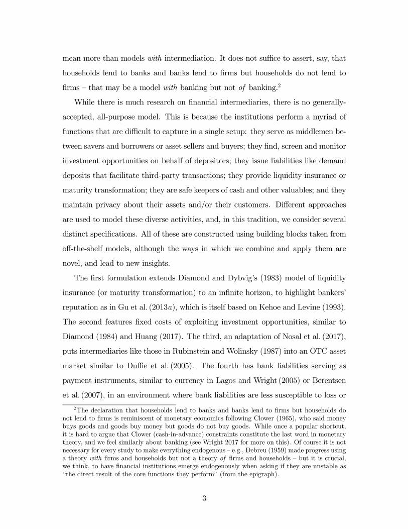
mean more than models with intermediation. It does not suffice to assert, say, that

households lend to banks and banks lend to firms but households do not lend to

firms — that may be a model with banking but not of banking.2

While there is much research on financial intermediaries, there is no generally-

accepted, all-purpose model. This is because the institutions perform a myriad of

functions that are difficult to capture in a single setup: they serve as middlemen be-

tween savers and borrowers or asset sellers and buyers; they find, screen and monitor

investment opportunities on behalf of depositors; they issue liabilities like demand

deposits that facilitate third-party transactions; they provide liquidity insurance or

maturity transformation; they are safe keepers of cash and other valuables; and they

maintain privacy about their assets and/or their customers. Different approaches

are used to model these diverse activities, and, in this tradition, we consider several

distinct specifications. All of these are constructed using building blocks taken from

off-the-shelf models, although the ways in which we combine and apply them are

novel, and lead to new insights.

The first formulation extends Diamond and Dybvig’s (1983) model of liquidity

insurance (or maturity transformation) to an infinite horizon, to highlight bankers’

reputation as in Gu et al. (2013a), which is itself based on Kehoe and Levine (1993).

The second features fixed costs of exploiting investment opportunities, similar to

Diamond (1984) and Huang (2017). The third, an adaptation of Nosal et al. (2017),

puts intermediaries like those in Rubinstein and Wolinsky (1987) into an OTC asset

market similar to Duffie et al. (2005). The fourth has bank liabilities serving as

payment instruments, similar to currency in Lagos and Wright (2005) or Berentsen

et al. (2007), in an environment where bank liabilities are less susceptible to loss or

2The declaration that households lend to banks and banks lend to firms but households do

not lend to firms is reminiscent of monetary economics following Clower (1965), who said money

buys goods and goods buy money but goods do not buy goods. While once a popular shortcut,

it is hard to argue that Clower (cash-in-advance) constraints constitute the last word in monetary

theory, and we feel similarly about banking (see Wright 2017 for more on this). Of course it is not

necessary for every study to make everything endogenous — e.g., Debreu (1959) made progress using

a theory with firms and households but not a theory of firms and households — but it is crucial,

we think, to have financial institutions emerge endogenously when asking if they are unstable as

“the direct result of the core functions they perform” (from the epigraph).

3

theft, as in He et al. (2007) and Sanches and Williamson (2010), or less sensitive

to information, as in Andolfatto and Martin (2013), Dang et al. (2017) and others

mentioned below.

We find in each case that financial intermediation can indeed engender instability:

an economy with these institutions is more likely to have multiple equilibria or

volatile dynamics than the same economy without them. In some cases there is a

unique equilibrium, and it is stable, without intermediation, but multiple or volatile

equilibria with it; in other cases both can have multiple or volatile equilibria, but

intermediation expands the set of parameters for which this is the case. Further,

while the economic logic differs across models, in each case the results are directly

related to the raison d’etre for intermediation.

As the literature on intermediation is vast, we refer to standard sources (e.g.,

Freixas and Rochet 2008; Calomiris and Haber 2014; Vives 2016). We do mention

Shleifer and Vishny (2010), which has a similar motivation, even if our methods are

different, coming mainly from monetary theory (e.g., Lagos et al. 2017; Rocheteau

and Nosal 2017). Thus, we use infinite-horizon models, since we are interested in

economic dynamics, and, moreover, finite-horizon models are ill suited for capturing

salient features of financial activity, including unsecured credit, reputational con-

siderations and the use of money. We also use general equilibrium, in the sense of

logically closed systems, making as few as possible exogenous restrictions on prices,

contracts or behavior. This is to see if instability arises from intermediation per se

and not extraneous features like noise traders, sticky prices, irrational expectations

etc. To be clear, we have frictions like limited commitment, imperfect informa-

tion/communication, and spatial/temporal separation, but those are imposed on

the environment, not on prices, contracts or behavior. Thus, we think, what follows

are models of financial intermediation, not just with financial intermediation.3

3Anticipating some readers might find four models more than they want to see in one paper,

to rationalize this, the point is that the results are robust to different ways of formalizing the roles

of financial intermediaries. We revisit that point in the Conclusion, where we also discuss the

common thread across the different environments. Moreover, as the presentation of each model is

self contained, readers could pick and choose without loss of continuity.

4

Model 1: Insurance

Our various specifications are novel, but all make use of standard building blocks

from the literature that have been deemed relevant for banking. The first one

extends Diamond and Dybvig’s (1983) popular model to an infinite horizon. As in

Gu et al. (2013a), this lets us incorporate reputational considerations à la Kehoe

and Levine (1993).

Time is discrete and infinite. Some agents live forever, while at each date a [0 1]

continuum of other agents are around only for that period — a simple way to make

them care less about reputation (in principle, they can be around for any ∞periods, but = 1 is obviously easiest). Each period has two subperiods. The

short-lived agents are homogeneous ex ante but face idiosyncratic shocks: they are

impatient with probability and patient with probability 1 − , where impatient

(patient) agents derive utility only from consumption in the first (second) subperiod.

Given the shock, which is private information, they have utility (), = 1 2,

where is consumption in subperiod , with 0 0 and 00 0.4 Infinite-lived

agents have period utility () for in either subperiod, with 0 0, 00 ≤ 0 = (0).

Short-lived agents have an endowment of 1; infinitely-lived agents have 0. The

standard technology is this: a unit of the good invested at the start of the first

subperiod yields 1 units in the second subperiod; or, the investment can be

terminated at the end of the first subperiod to get back the input.5 The good can

also be stored one-for-one across subperiods. As in any Diamond-Dybvig model, to

insure against the shocks, the short-lived agents can form a coalition that resembles

a banking arrangement. Thus, they design a contract (1 2) to solve

max12

{1 (1) + (1− )2 (2)} (1)

st (1− ) 2 = (1− 1) (2)

2 ≥ 1 (3)

4Many applications of Diamond-Dybvig assume 1 (·) = 2 (·), but not all (e.g., Peck and Shell2003). The flexibility of the general version is useful for constructing examples.

5See Andolfato et al. (2019) for a version of Diamond-Dybvig with a security market, where

early termination entails a cost, which similarly implies it reduces the return on investment.

5

where (2) is feasibility and (3) is a truth-telling constraint (if 2 1 patient agents

would claim to be impatient, get 1 and store it to the next subperiod). There are

also nonnegativity constraints omitted to save space.

This problem is well understood. One result is: assuming 01 (1) 02 () and

01 () ≤ 02 () at = (1− + ), we get 1 ∗1 ∗2 , so (3) is not

binding, and full insurance/efficiency obtains. However, this requires commitment;

otherwise, when they learn they are patient and are supposed to make transfers

to the impatient, agents will renege. Given our short-lived agents cannot commit,

naturally, there emerges a role for long-lived agents as bankers who accept deposits,

invest them, and pay off depositors on demand at terms to be determined. Impor-

tantly, bankers do not have exogenous commitment ability — it is endogenous and

based on reputation. Thus, bankers honor obligations lest they get identified as

renegers, whence they are punished to autarky, which is a credible threat because

there are many perfect substitutes for any given banker.

However, a banker may be tempted to misbehave as in the “cash diversion”

models in Biais et al. (2007) or DeMarzo and Fishman (2007): if he misappropriates

deposits, he gets payoff , where is not too big, so this is socially inefficient, but

he might do it opportunistically. As in Gu et al. (2013a,b), the risk is that he gets

caught, and punished, with probability ≤ 1, where one interpretation is that isthe probability one generation of depositors can communicate his misbehavior to the

next generation.6 Now depositors may set 1, and invest 1− on their own, to

reduce bank incentives to misbehave, different from most papers that simply assume

= 1, but similar to Peck and Setayesh (2019). In addition to , the contract now

specifies payouts per deposit contingent on withdrawal time , = 1 2, and the

banker’s income ∈ [0 ], which he invests for utility ().Since there is more than one long-lived agent, the short-lived agents can choose

any of them to act as banker, and in the spirit of Diamond-Dybvig they make

this choice as a coalition. However, we assume they can choose only one, to avoid

6While = 1 is fine, it does not simplify things much, and it is known from other applications

that 1 can be interesting (e.g., the extension of Kocherlakota 1998 in Gu et al. 2016).

6

determining the optimal number of bankers, something we do in Model 2, but would

be a distraction here; it can be rationalized by assuming that it is too costly to

monitor more than one banker. Still, since they can choose any one, for reasons

often summarized as Bertrand competition the contract maximizes the expected

utility of the depositors. Yet a banker may get a positive surplus — a rent on his

option to act opportunistically — because the contract must give him incentives to

not misuse deposits for his own gain.

The banker’s incentive constraint is

() + +1 ≥ + (1− )+1 (4)

where is his discount factor, is his equilibrium payoff, and the RHS is the

deviation payoff, including for sure and +1 iff he is not caught. Note that +1

is his valuation next period, facing a new generation of depositors, and hence is taken

as given when designing a contract at . Also note that bankers do not misuse on

the equilibrium path, but if one were to, he would get but not ()+ (− ).

This leads to the contracting problem

max12

{1 (1 + 1− ) + (1− )2 [2 + (1− )]} (5)

st (1− ) 2 = ( − − 1) (6)

2 ≥ 1 (7)

− () ≤ (8)

where (8) rewrites (4) using ≡ +1. Note that is a bank’s franchise value,

capturing the banker’s reputation for trustworthiness. Substituting (6) into (5) to

eliminate 2, ignoring subscripts for now, and taking FOC’s wrt (1 ) we get

1 : { [01 (1)−02 (2)]− 1 (1− +)} 1 = 0 : {(1 − 1) [01 (1)−02 (2)] + 1 [− (1− +) 1]− 2} = 0 : [−02 (2)− 1 + 2

0 ()] = 0

where 1 = 1 + 1− and 2 = 2 + (1− ), while 1 and 2 are multipliers for

constraints (7) and (8).

7

These FOC’s yield two critical values, ∗ 0 and ∗, delineating three

regimes: (i) If ≥ ∗ then (8) is slack, and = 0, since the franchise value keeps

the banker honest without 0. In this case there is a continuum of contracts

achieving the full-insurance outcome, because depositors can have the bank invest a

lot or a little, and in the latter case invest the rest on their own (exactly as in Peck

and Setayesh 2019). (ii) If ∈ [ ∗) we must either lower ∗ or raise 0

to satisfy (8). While lowering from ∗ means less-than-full insurance, this is a

second-order cost by the envelope theorem, so the contract sets = and keeps

= 0. (iii) If , lowering further entails too much risk, so it sets 0. In

case (i), one of the payoff-equivalent contracts has 1 = 2, and (ii)-(iii) the unique

contract has 1 = 2; hence wlog we set 1 = 2 = from now on.

In regime (iii), ( ) satisfies

= [− (1− +) ] (9)

= − () (10)

02 (2)01 (1)−02 (2)

=

1− +

∙(− 1) (1− )

0 ()− 1

¸(11)

with 1 = 1−+(− ) (1− +), 2 = (1− )+(− ) (1− +).

These and the analogs from regimes (i)-(ii) characterize the contract given , and in

particular, one can easily check 0 () 0 ∀ , which is important below. This

is shown in Fig. 1 for the following parameterization:7

Example 1: Let () = ,

1 (1) = 1(1 + )

1−1 − 1−1

1− 1and 2 (2) = 2

(2 + )1−2 − 1−2

1− 2

where = 095, 1 = 2 = 2, = 001, 1 = 1, 2 = 01, = 21, = 07,

= 025, = 06 and = 099.

As mentioned, the contract takes as given. To embed this in general equilib-

rium, use ≡ +1 to write = () + +1 as a dynamical system,

−1 = () ≡ [ ()] + (12)

7Notice 0 here (in fact, for the example = 03257 and ∗ = 0600); the case 0 is less

interesting because it never has banking in steady state. In terms of primitives, one can show that

0 iff [01 (1)−02 ()] [(− 1) (1− ) 0 (0)− ] 02 () (1− +)

8

Figure 1: Model 1, bank contract vs

where () comes from the contracting problem. Equilibrium is defined as a nonneg-

ative, bounded path for solving (12), from which the other endogenous variables

follow using the FOC’s. A stationary equilibrium, which is the same as a steady

state here, solves = ¡¢. The nature of steady state depends on whether ≤ 0

or 0 (conditions for which are given in fn. 7). Appendix A proves:

Proposition 1 If ≤ 0 the unique steady state has no banking, = 0. If 0

the unique steady state has ∈ (0 ) and banking, 0.

For dynamic equilibria, first note from (12) that () has a linear term that

is increasing and a nonlinear term that is decreasing because 0 () 0. If the

net effect implies 0 () 0 over some range the system can exhibit nonmonotone

dynamics. For Example 1, Fig. 2a shows and −1, which cross on the 45 line at

= 03215. In this case the system is monotone and there is a unique equilibrium,

which is the steady state, because that is the only bounded path solving (12). To

see this is not true in general consider:

Example 2: Same as above except 1 = 10 and = 1

As Fig. 2b shows, now 0() −1, and so and −1 intersect not only on the

45, but also off it, at ( ) and ( ) with = 00696 and = 00689. As

is standard (see Azariadis 1993), this means there is a two-cycle equilibrium where

oscillates deterministically between and . It also means there are sunspot

9

equilibria where fluctuates randomly between values close to and (see

Appendix B). Thus we can get deterministic or stochastic volatility with banking

and not without it. That does not mean banking is a bad idea, as it provides

insurance to agents who cannot insure each other, due to commitment issues. It

does mean banking can engender instability.

Figure 2a: Model 1, monotone Figure 2b: Model 1, nonmonotone

Figure 3: Model 1, time series for a two-cycle

The intuition is straightforward: if next period +1 is high then this period

is high and we can discipline bankers with low ; but that makes the current and

hence −1 low. This induces a tendency towards oscillations, but for a cycle the

effect has to dominate the linear term in (), which is why parameters matter.

Fig. 3 plots time series of ( ) over the cycle in Example 2. Notice moves

with and against . Whether moves with or against depends on parameters,

10

but here it is the latter. While the point is not to take this example seriously

in a quantitative sense, it is worth noting that the theory does make qualitative

predictions, and does not say “anything goes.”

Figure 4: Model 1, two- and three-cycles

Fig. 4 displays the existence of two-cycles in a different way, as fixed points of

the second iterate 2 = ◦ , for another parameterization:Example 3: = 1, 1 = 14, 2 = 15, = 001, 1 = 1, 2 = 0075, = 22,

= 1, = 028, = 075 and = 076.

Notice 2 has three fixed points, , plus and from the two-cycle. Also shown

is 3, which has seven fixed points, plus a pair of three-cycles. Standard results

(again see Azariadis 1993) say the existence of three-cycles implies the existence of

−cycles for any integer , plus chaos, which is basically a cycle with =∞.To summarize, banking can introduce many equilibria, including deterministic,

stochastic and chaotic dynamics, directly attributable to the idea that banks depend

on trust, and at least to some extent that is a self-fulfilling prophecy.

Model 2: Delegated Investment with Fixed Costs

The next formulation has intermediation originating from economies of scale,

based on Diamond (1984) and Huang (2017) (see also Leland and Pyle 1976 or

Boyd and Prescott 1986 on the bigger picture). Time is discrete and continues

forever as in Model 1, but here all agents are infinitely lived. Also, they are now

11

spatially separated — say, across a large number of islands — and randomly relocated

at the end of each period, following a literature on banking including Champ et

al. (1996), Bencivenga and Smith (1991), Smith (2002) and Bhattacharya et al.

(2005).8 Economies of scale are captured as follows: agents must pay a fixed cost ,

in terms of goods, to locate/evaluate/monitor investment projects, after which any

project returns per unit invested.

Period utility is () − (), where is consumption and investment (say,

output produced one-for-one with labor) where 0 0 0 and 00 ≥ 0 00. Also,

0 (0) 0 (0), so that agents invest if = 0. Normalize (0) = (0) = 0. If 0

the payoff is

1 = max

{ ()− ()} st = − (13)

from investing on one’s own (omitting nonnegativity constraints as above). Suppose

is too high to support this, so 1 0, while the autarky payoff is 0 = 0. Now

consider agents forming a coalition where some, that we call depositors, delegate

their investment to others, that we call bankers, to share the fixed cost.

As is standard in models with nonconvexities, the coalition uses a lottery to

chose a subset of members to act as bankers.9 Thus, is the probability of being a

banker, equal to the measure of bankers if the island population is normalized to 1.

As in Model 1, bankers have the option to misbehave, with and playing similar

roles. The relevant incentive condition is therefore

+1 ≥ (1− )

+ (1− )+1 (14)

where the RHS is the deviation payoff, given each depositor is promised and

8The main function of random relocation here is to let us avoid long-term contracting con-

siderations, which are interesting but complicated (e.g., in Gu et al. 2013a, bankers’ rewards can

be backloaded over multi-period contracts). Elsewhere in the paper we avoid those issues using

short-lived agents, but here we want all agents to be long-lived, so that ex ante anyone can po-

tentially be a banker. In any case, it is important to emphasize that these are not restrictions

on contracting per se, but assumptions on the environment that impinge on the contract. Does

it matter? Yes, because without making them explicit one cannot know, in general, how these

assumptions impinge on all endogenous variables.9This is similar to, e.g., Rogerson’s (1988) indivisible-labor model, except unlike his, our agents

cannot commit, so our contracts must be incentive compatible before and after the lottery.

12

each banker controls (1− ) of the resources.10 The trade-off, as emphasized

in Huang (2017), is that having fewer banks saves on fixed costs but raises their

temptation to misbehave, because they must be larger, given total deposits.

The contract maximizes the payoff to the representative agent on an island

() = max

{ [ ()− ()] + (1− ) [ ()− ()]} (15)

st + (1− ) = [ + (1− ) ]− (16)

()− () ≥ 0 (17)

1−

≤ (18)

where ≡ +1, while () and ( ) are the consumption/investment

allocations of bankers and depositors. Here (16) is the resource constraint, (17) is

the incentive constraint for depositors, and (18), which rewrites (14), is the incentive

constraint for bankers.

Substituting (16) into (15) to eliminate , and letting and be multipliers,

we get the FOC’s:

: 0 ()− 0 () = 0

: (1− ) [0 ()− 0 ()]− 0 () = 0

: (1− ) [0 ()− 0()] + 0 ()− 1−

= 0

:

½ ()− ()− [ ()− ()] + 0 ()

−

+

2

¾= 0

One can check 0 () ≥ 0. Moreover, (0) = 0, so we get no banking at = 0.

In the limit as → ∞ we get → 0, which means very few banks but they are

huge. Also as →∞ we get ()→ ∗ ≡ max [ ()− ()] st = , which

totally dissipates the fixed cost (i.e., delivers the same payoff as = 0).

Fig. 5 shows the contract given for the following parameterization:

Example 4: Let

() = (+ )

1− − 1−

1− and () =

10Here we assume that a deviating banker receives ()− () in addition to [(1−)],

slightly different from Model 1. In both cases, these assumptions are made mainly for convenience,

and neither one is unambiguously better.

13

with = = 0001, = 2, = 01, = 230, = 12, = 076, = 095 and

= 9.

Notice that there is a cutoff , which is = 00182 in this example, and banking is

viable iff ≥ .

Figure 5: Model 2, bank contract vs

To embed this in equilibrium use = () + +1 and emulate the methods

from Model 1 to get

= ¡+1

¢ ≡

¡+1

¢+ +1 (19)

Equilibrium is a bounded, nonnegative solution to (19). Notice () = for

≤ , and () for big due to the fact that ≤ ∗. Then we have:

Proposition 2 There is a steady state at = 0, without banking. There can be

steady states with banking, generically an even number that alternate between stable

and unstable.

Fig. 6 shows Example 4 has three steady states, = 0, plus two with banking,

2 1 0. This is different from Model 1, which has a unique steady state , and

has nonstationary equilibria iff 0¡¢ −1. Now 0 () 0, so deterministic cycles

are impossible, but if there are multiple steady states we can use a different approach

to construct sunspot equilibria around the stable ones.11 Appendix B shows there

11To give credit where credit is due, in Model 2 we use the method in Azariadis (1981), while

in Model 1 we use the method in Azariadis and Guesnerie (1986).

14

are equilibria where fluctuates between and for any ∈ (0 1) and ∈ (1 2). In particular, means we switch stochastically between 0

and = 0 — i.e., random episodes of crises, where deposits dry up and banking

shuts down, due to sunspots, which are fundamentally irrelevant events. This is

again different from Model 1, where can fluctuate, but only with 0 ∀.

Figure 6: Model 2, monotone with multiple steady states

While Models 1 and 2 are different, in terms of economics and mathematics,

Appendix C presents an environment that integrates elements of both. It has two

agents on each island, one that is infinitely lived and one that is only around for

one period, who negotiate the contract using generalized Nash bargaining (having

just two is simpler, but we also considered many depositors and one banker, with

multilateral bargaining, and got similar results). There are gains to delegating

investment due to 0, as in Model 2, but only long-lived agents can act as

bankers, as in Model 1. Letting denote bankers’ bargaining power, we get a

dynamical system = ¡+1

¢that can be nonmonotone for 1. Appendix C

shows we can have multiple steady states, with 0 () 0 around the stable ones

and hence sunspot equilibria as in the benchmark Model 2, as well as 0 () −1around the unstable steady states and hence cycles and sunspots as in Model 1.

The reason () is decreasing in Appendix C is the following well-known (see

Kalai 1977) feature of Nash bargaining: agents with bargaining power 1 can

15

get a smaller surplus when the bargaining set expands. Here this is manifest in

bankers’ surplus falling with , similar to 0 () 0 in Model 1. That does not

happen in the baseline Model 2, where agents in the coalition are ex ante identical

and hence treated symmetrically, so they all get a bigger surplus when increases.

Details aside, the point is that there are distinct ways to formalize how banking

might engender instability in models based on reputation/trust.12

Model 3: Asset Market Intermediation

Banks are not the only interesting financial intermediaries. Work following Duffie

et al. (2005) studies asset markets using search theory, where agents may trade with

each other, or with middlemen/dealers that buy from those with low asset valu-

ation and sell to those with high valuation. We pursue this with a few changes

in their environment. In particular, most papers following Duffie et al. (2005) give

middlemen continuous access to a frictionless interdealer market (with some excep-

tions, e.g., Weill 2007, but they do not study the issues analyzed here). Hence,

their intermediaries do not hold assets in inventory. Our middlemen are more like

those in Rubinstein and Wolinsky (1987), who buy goods from producers and hold

inventories until they randomly sell to consumers. However, here they trade as-

sets and not goods, which matters. The following presentation builds on Nosal et

al. (2017), although we amend their setup in many ways, including: adding het-

erogenous projects; modifying the market composition conditions (see fn. 13); and

switching from continuous to discrete time. All of these affect the results.

There are large numbers of three risk-neutral types, , and , for asset

buyers, sellers and middlemen. Type agents stay in the market forever, while

type and stay for one period (we also studied alternatives, like letting everyone

stay forever, with similar results). Upon exit and are replaced by “clones” to

maintain stationarity (a device borrowed from Burdett and Coles 1997). Type

agents, sometimes called end users, want to acquire an asset — let’s call it capital —

12Model 1 can be interpreted as bargaining where banks have = 0. Hence, one may conjecture

that dynamics like those in Appendix C emerge in Model 1 if we allow ∈ (0 1), but then Model1 becomes intractable; the setup in Appendix C is relatively quite tractable.

16

to implement a project for profit 0, where is observable when agents meet,

but random across end users with CDF given by (). The originators of capital,

type , if they enter the market each bring 1 indivisible unit; those that stay out

put their capital to alternative uses, defining their opportunity cost of participation,

denoted 0, which for simplicity is the same for all .

Type agents, who are always in the market, can acquire capital from , but as

usual in these models their inventories are restricted to ∈ {0 1} (with exceptions,e.g., Lagos and Rocheteau 2009, but they do not study the issues analyzed here).

Let be the measure of type at with = 1. Capital held by depreciates

by disappearing each period with probability ≥ 0, but while he holds it gets

a return 0. His crucial choice is then, if he has = 1 and meets , should he

trade or keep for himself? This depends on fundamentals, of course, including the

end user’s , but as we show below, it can also depend on beliefs.

Market composition is determined as follows: the measures and of types

and are fixed, but entry by makes endogenous.13 Given this, the meeting

technology is standard: each period everyone in the market contacts someone with

probability , and each contact is a random draw from the participants. In partic-

ular, if is the total measure of participants then types and both meet type

with probability , so has no advantage over in that regard.14 When

and meet they trade for sure since this is ’s only chance and cost is sunk.

Similarly, when meets with = 0 they trade for sure. When with = 1

meets , however, they may or may not trade.

As regards prices, if type gives capital the latter pays (in terms of trans-

ferable utility) determined by bargaining. Thus, if Σ is the total surplus available

13Entry by is nice because it lets us compare economies with the same entry conditions with

and without middlemen. Still, results for entry by are given in Appendix D; entry by is less

interesting and hence omitted. These alternatives are all better than Nosal et al. (2017), where

agents choose to be either type or . That is awkward because in cyclic equilibria they switch

back and forth over time between being and . Here no one switches, but participation by a

type can vary, as in conventional search theory (e.g., Pissarides 2000).14This is different from the original Rubinstein-Wolinsky setup, which is based entirely on

being better than at search; we could allow that, too, but do not need it.

17

when and meet, as long as Σ 0 they trade, and type ’s surplus is Σ,

where ∈ [0 1] is his bargaining power. To flesh this out, let and be

value functions for types and ; let be the value function for when he has

∈ {0 1}; and let ∆ = 1 − 0 be ’s gain from having inventory. Then

Σ = , Σ = (1− )∆+1, Σ = − (1− )∆+1

where ∈ (0 1) is ’s discount factor.15 Bargaining then yields

= , = (1− )∆+1, = + (1− )∆+1 (20)

When with = 1 and with project meet, they trade with probability

= (), where

() =

⎧⎨⎩ 0 if

[0 1] if =

1 if

(21)

and ≡ (1− ) ∆+1 is the reservation value of a project making Σ = 0. Hence,

the market payoff for with project is

() =

+

() [ − (1− )∆+1] (22)

The first term on the RHS is the probability meets , times his share of the

surplus; the second is the probability he meets with = 1, times the probability

they trade, times his share of the surplus; and note prices do not appear since they

were eliminated using (20). Similarly, the market payoff for is

=

Z ∞

0

() +( − )

(1− )∆+1 (23)

The payoff for depends on inventory. Using = (1− )∆+1, we have

0 =

+ 0+1 (24)

1 = +

Z ∞

( −) () + (1− )1+1 + 0+1 (25)

15Note there are no continuation values or threat points for and , as they are in the market

for just one period, but while that simplifies some algebra it is not otherwise important.

18

Subtracting and simplifying with integration by parts, we get

−1 = (1− )

½+ +

Z ∞

[1− ()] −

¾ (26)

giving the evolution of over time. The evolution of inventories held by is

+1 = (1− )

∙1−

E ()¸+( − ) (1− )

(27)

where E () = ( ) is the unconditional probability that and

trade. The first term on the RHS is current times the probably a unit of does

not depreciate or get traded; the second is current − times the probability

acquires and it does not depreciate.

We can eliminate in (26)-(27) using ’s entry condition, = , which

reduces to

=E + ( − )

− − (28)

What’s left is a two-dimensional dynamical system that is compactly written as∙+1−1

¸=

∙( )

( )

¸ (29)

Given an initial 0, equilibrium is a nonnegative, bounded path for ( ) solving

(29).16

With no intermediaries, = 0, the equilibrium is basically static and it is easy

to check that it is unique. With 0, first note that the locus of points satisfying

= (), called the -curve, and the locus satisfying = (), called the

-curve, both slope up in () space. Then, to develop some intuition, consider

the special case where = is constant. As shown in Fig. 7, for this case there are

three possible regimes: (i) , so with = 1 and trade with probability

= 1; (ii) , so they trade with probability = 0; and (iii) = , so they

trade with probability ∈ (0 1). Appendix A proves:16A distinction between this model and others in the paper is that this system is two dimensional:

is a jump variable, like in the previous sections, while is a (predetermined) state variable,

so transitions are nontrivial. The version of Model 3 in Appendix D, with entry by instead

of , is different: there one can solve a univariate system −1 = () to get the path for ,

after which , etc. follow from simple conditions. Intuitively, with entry by (entry by )

the model is (is not) block recursive, as discussed in Shi (2009). Hence, Appendix D delivers more

results, including chaotic dynamics, but we still prefer entry by as a benchmark model.

19

Proposition 3 With = there exist 0 and such that: (i) if ∈ [0 )there is a unique steady state and it has ; (ii) if ∈ (∞) there is a uniquesteady state and it has ; (iii) if ∈ ( ) there are three steady states, ,

, and = .

Figure 7: Model 3, phase plane

For several reasons we prefer a nondegenerate ().17 So, consider a smooth

mean-preserving spread of the degenerate case, leading to the shown in phase plane

Fig. 8.

Example 6: Let

() =

⎧⎨⎩ 10 if 0 ≤ ≤ 01 + (3 − 1) ( − 0) (2 − 0) if 0 ≤ 22 + (1− 3) ( − 2) (4 − 2) if 2 ≤ 4

(30)

with 0 = 099, 1 = 005, 2 = 101, 3 = 095 and 4 = 2. Also, let = 1,

= 01, = 005, = 05, = 05, = 1, = 07, = 1104, = 0008

and = 02.

17For the nondegenerate () studied below, the flat portion of the -curve in Fig. 7 is elimi-

nated. Then in any steady state and are indifferent to trade only in the rare event = , in

contrast to the mixed-strategy equilibrium in the degenerate case, where they are always indifferent.

Moreover, with nondegenerate (), if varies across pure-strategy steady states intermediation

activity does too, but not necessarily to the extreme extent of the degenerate case, where it is

either = 1 or = 0. Similarly, for real-time dynamics, cycles with nondegenerate () have

fluctuations in intermediation activity but not necessarily between = 0 and = 1.

20

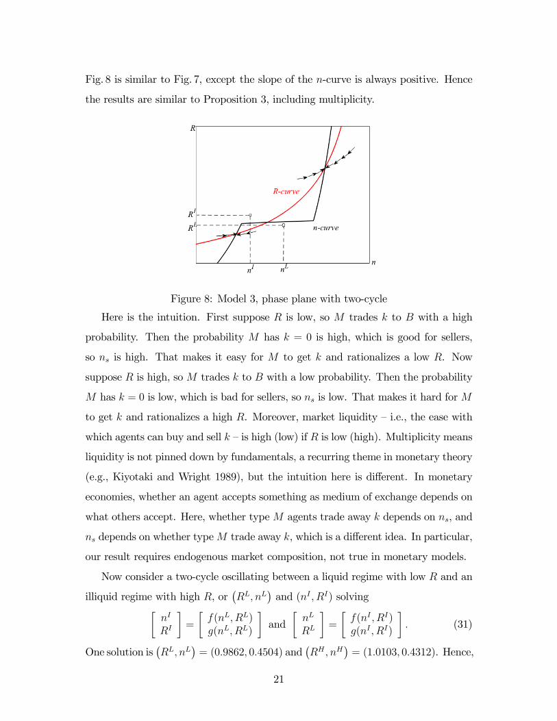
Fig. 8 is similar to Fig. 7, except the slope of the -curve is always positive. Hence

the results are similar to Proposition 3, including multiplicity.

Figure 8: Model 3, phase plane with two-cycle

Here is the intuition. First suppose is low, so trades to with a high

probability. Then the probability has = 0 is high, which is good for sellers,

so is high. That makes it easy for to get and rationalizes a low . Now

suppose is high, so trades to with a low probability. Then the probability

has = 0 is low, which is bad for sellers, so is low. That makes it hard for

to get and rationalizes a high . Moreover, market liquidity — i.e., the ease with

which agents can buy and sell — is high (low) if is low (high). Multiplicity means

liquidity is not pinned down by fundamentals, a recurring theme in monetary theory

(e.g., Kiyotaki and Wright 1989), but the intuition here is different. In monetary

economies, whether an agent accepts something as medium of exchange depends on

what others accept. Here, whether type agents trade away depends on , and

depends on whether type trade away , which is a different idea. In particular,

our result requires endogenous market composition, not true in monetary models.

Now consider a two-cycle oscillating between a liquid regime with low and an

illiquid regime with high , or¡

¢and ( ) solving∙

¸=

∙( )

( )

¸and

∙

¸=

∙( )

( )

¸ (31)

One solution is¡

¢= (09862 04504) and

¡

¢= (10103 04312). Hence,

21

we have real-time dynamics (not just multiple steady states) with excess volatility

in liquidity, trade volume, prices and quantities. Fig. 9 shows the times series. In

the liquid regime: is low, making more inclined to trade with ; is high,

because and traded less last period; and is low, because low and high

discourage entry by . The illiquid regime has the opposite properties.

Figure 9: Model 3, time series for a two-cycle

We do not claim that actual data are best explained by a two-cycle, but suggest

if such a simple model can deliver equilibria where endogenous variables vary over

time, as self-fulfilling prophecies, it lends credence to the notion that intermediated

asset markets in the real world might be prone to similar instability.18

Model 4: Safety and Secrecy

An important role of banks is the issuance of liabilities that facilitate third-

party transactions. Indeed, for the general public, that is virtually their defining

characteristic: “banks are distinguished from other kinds of financial intermediaries

18Prices are also shown in Fig. 9 (averaged over when trades). The price pays is

constant over time, as it depends only on fundamentals, but the price pays or pays

moves with . The spread can go either way, but here it moves against . This is all broadly

consistent with the data discussed in Comerton-Forde et al. (2010), and other stylized facts (e.g.,

inventories are volatile than output). While this is obviously not a calibration, the finding that it

is qualitatively more consistent with observations may lend further credence to the story.

22

by the readily transferable or ‘spendable’ nature of their IOUs, which allows those

IOUs to serve as a means of exchange, that is, money... Commercial bank money

today consists mainly of deposit balances that can be transferred either by means

of paper orders known as checks or electronically using plastic ‘debit’ cards” (Selgin

2018). We pursue this idea in a model with an explicit need for payment instruments,

building on the New Monetarist framework surveyed by Lagos et al. (2017) and

Rocheteau and Nosal (2017), where we introduce banks in two related ways.

In Model 4a, bank liabilities are safe relative to other assets in the sense that

they are less susceptible to theft or loss (similar to He et al. 2007; see also Sanches

and Williamson 2010). Traveler’s checks are a case in point but not the only one —

in general, it is obviously worse to have your cash lost or stolen than your checkbook

or debit card. Also, if merchandise turns out to be fraudulent or defective, which is

similar to theft, it is typically easier to stop payment if you use a check or credit card

than if you use cash.19 Model 4b builds on the idea that payment instruments orig-

inating with banks can be, as Dang et al. (2017) put it, informationally insensitive

when these institutions act as secret keepers; an earlier exposition of this is Gorton

and Pennachi (1990) while Andolfatto and Martin (2013), Andolfatto et al. (2014),

Loberto (2017), and Monnet and Quintin (2017) are versions that go deeper into

the microfoundations.20

While there are different approaches to modeling media of exchange, one based

on Lagos and Wright (2005) is convenient for both Models 4a and 4b. In that setup,

in each period of discrete time two markets convene sequentially: a decentralized

market, or DM, with frictions detailed below; and a frictionless centralized market,

or CM. There are two types of infinitely-lived agents, a measure 1 of buyers and

19Safety was a critical feature of banks historically. Consider the British goldsmiths: “At first

[they] accepted deposits merely for safe keeping ; but early in the 17th century their deposit receipts

were circulating in place of money” (Encyclopedia Britannica, quoted in He et al. 2005; emphasis

added). Also, “In the 17th century, notes, orders, and bills (collectively called demandable debt)

acted as media of exchange that spared the costs ofmoving, protecting and assaying specie” (Quinn

1997; emphasis added). Safety was also crucial for earlier bankers, including the Templars (Sanello

2003), who specialized in moving purchasing power over dangerous territory.20Other models of bank liabilities circulating as media of exchange that are similar in spirit but

very different in detail include Cavalcanti and Wallace (1999a,b) and Cavalcanti et al. (1999).

23

a measure of sellers. Their roles differ in the DM, but they are similar in the

CM, where they all trade a numeraire consumption good and labor for utility

()− , with 0 0 00. They also trade assets in the CM, like the trees in the

standard Lucas (1978) model, giving off a dividend 0 in the CM in numeraire.

All agents discount by ∈ (0 1) between one CM and the next DM, but wlog they

do not discount between the DM and CM.

In the DM agents meet bilaterally, where sellers can provide a good (different

from ) that buyers want. Let be the probability a buyer meets a seller, so that

is the probability a seller meets a buyer. In any meeting, if a seller produces for

a buyer the former incurs cost () and the latter gets utility (), where (0) =

(0) = 0, 0 0 0 and 00 ≥ 0 00. Also, let ∗ satisfy 0 (∗) = 0 (∗). Goods

and are nonstorable, so they cannot serve as commodity money. Credit is not

viable because there is limited commitment and DM trading is anonymous. Hence,

as is standard in these models, sellers only produce if they get assets in exchange.

Let the terms of trade be given by a generic mechanism, as in Gu and Wright

(2016), meaning this: for a buyer to get , he must give the seller assets worth () in

CM numeraire, for some function with (0) = 0 and 0 () 0. A simple example

is Kalai’s (1977) proportional bargaining solution, () = () + (1− ) ().

Generalized Nash is similar but the formula for () is more complicated when

liquidity constraints are operative. For a fairly general class of mechanisms, Gu

and Wright (2016) show this: if a buyer has enough assets to make his liquidity

constraint slack, he gets the efficient = ∗ and pays ∗ = (∗); but if he has assets

worth ∗, he gives them all to the seller and gets = −1 () ∗.

In Model 4a, assets can be held in forms that differ in safety and liquidity,

where safety is captured by the probability of being stolen (or lost), and liquidity is

captured by whether it can be used as means of payment in the DM. To maintain

stationarity, any assets that are stolen (or lost) return to the system next period,

say because thieves (or finders) bring them to the CM. Let a =(1 2) be a buyer’s

portfolio: 1 denotes assets held in a safe but illiquid form, say hidden in one’s

24

basement, meaning that it cannot be stolen (or lost) but also cannot be used in the

DM; and 2 denotes assets held in a liquid form, which means they are brought to

the DM, where can be used as payment instruments, but there is a probability 0

of being stolen (or lost).

The ex dividend price of the asset in terms of numeraire is independent of

whether it is held as 1 or 2. A buyer’s CM value function is () where =

(+)Σ is wealth. His DM value function is (a), which depends on his portfolio

and not just its value. A buyer’s CM problem is then

() = maxa

{()− + (a)} st = + − Σ

where a = (1 2) is his updated portfolio, and the CM real wage is 1 assuming

that is produced one-for-one with . Given an interior solution, several standard

results are immediate: (i) = ∗ solves the FOC 0(∗) = 1; (ii) a solves the

FOC’s +1 ≤ , = 0 if 0, which is independent of a, so all buyers

exit the CM with the same portfolio; and (iii) 0() = 1, so () is linear in

wealth. A seller’s CM problem (not shown) is similar, with a CM payoff again linear

in wealth.

A buyer’s value function is

+1(a) = (1− )n [ (+1)− (+1)] ++1(+1)

o+ +1[

¡+1 +

¢1]

where +1 is the wealth implied by a, with +1 solving (+1) =¡+1 +

¢2 if¡

+1 + ¢2 (∗), and (+1) = (∗) otherwise. The buyer’s surplus in a DM

transaction is () − (), because of the result that (·) is linear. Equilibriumis described by the Euler equations, which come from inserting the derivatives of

into the FOC’s from the CM:

0 = 1£¡+1 +

¢−

¤(32)

0 = 2©¡+1 +

¢(1− ) [1 + (+1)]−

ª (33)

where () = 0 () 0 ()− 1 0 is the liquidity premium on assets in the DM.

25

If we normalize the aggregate asset supply to 1, the dynamical system implied

by the model is described as follows. At any , there are three possible regimes: (i)

2 = 0; (ii) 0 2 1; and (iii) 2 = 1. In regime (i), inserting 1 = 1 and

2 = 0 into (32) and (33), we get = (+1 + ) and (1− ) [1 + (0)] ≤ 1,with the latter equivalent to

≥ ≡ (0)

1 + (0) (34)

Thus, agents bring no assets to the DM if the probability of theft is high.21 If (34)

holds, the DM shuts down, in which case the only possible equilibrium outcome has

= ∀, where ≡ (1− ) may be called the fundamental price of the

asset.22

Now assume , and consider regime (ii), where agents hold some but not

all their assets in liquid form. Inserting 1,2 0 into (32) and (33), we get

= ¡+1 +

¢and (1− ) [1 + (+1)] = 1, which means +1 = where

() =

1− (35)

One can show regime (ii) obtains iff +1 + 2¡+1 +

¢= () and .

Finally, consider regime (iii). Inserting 1 = 0 and 2 = 1 into (32) and (33),

we get ≥ ¡+1 +

¢and

= ¡+1 +

¢(1− ) [1 + (+1)] (36)

where +1 = −1(+1 + ) . This last condition is equivalent to +1 ≤ ≡ ()− . Hence if the dynamic system is =

¡+1

¢where:

() ≡½

( + ) (1− ) [1 + ◦ −1 ( + )] if

( + ) if ≥ (37)

Equilibrium is a nonnegative and bounded path for = ¡+1

¢.

21With Kalai bargaining and the Inada condition 0 (0) 0 (0) =∞, this reduces to = (1− + ), so = 1 if = 1 and 1 otherwise

22One might argue that (1− ) ( + ), and not ( + ), is the fundamental price, since an

asset holder only gets the return when it is not stolen. A rebutal is that someone always gets the

payoff, even if it is the thief. To avoid this semantic issue one can simply interpret as notation

for (1− ).

26

Proposition 4 Steady state exists, is unique, and is described as follows. Define

∈ [0 ) by =

◦ −1( + )

1 + ◦ −1( + ) (38)

Then (i) ≥ implies 1 = 1, 2 = 0 and = ; (ii) ∈ ( ) implies 1 0,

2 0 and = ; and (iii) ≤ implies 1 = 0, 2 = 1 and .

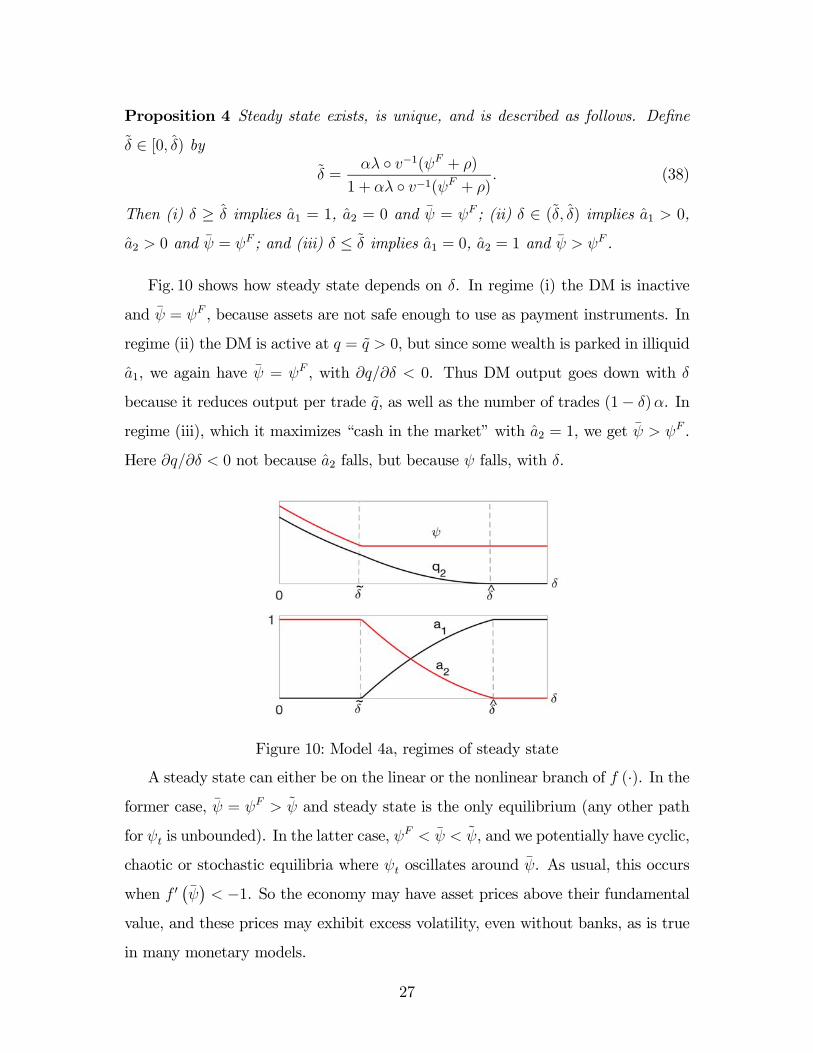
Fig. 10 shows how steady state depends on . In regime (i) the DM is inactive

and = , because assets are not safe enough to use as payment instruments. In

regime (ii) the DM is active at = 0, but since some wealth is parked in illiquid

1, we again have = , with 0. Thus DM output goes down with

because it reduces output per trade , as well as the number of trades (1− ). In

regime (iii), which it maximizes “cash in the market” with 2 = 1, we get .

Here 0 not because 2 falls, but because falls, with .

Figure 10: Model 4a, regimes of steady state

A steady state can either be on the linear or the nonlinear branch of (·). In theformer case, = and steady state is the only equilibrium (any other path

for is unbounded). In the latter case, , and we potentially have cyclic,

chaotic or stochastic equilibria where oscillates around . As usual, this occurs

when 0¡¢ −1. So the economy may have asset prices above their fundamental

value, and these prices may exhibit excess volatility, even without banks, as is true

in many monetary models.

27

Figure 11: Model 4a, dynamic equilibrium

Now introduce banks that take assets as deposits and issue receipts, claims on

these deposits. Let 3 denote assets on deposit, and assume they are safer than 2

but still liquid — i.e., as described in the above quotation from Selgin (2018), bank

liabilities (the receipts) are spendable.23 However, deposits may entail a lower yield

than the original assets, since banks may have operating costs and depositors may

be willing to sacrifice return for safety. If is the interest rate on deposits then bank

profit is

Π (3) = 3 (− )− (3) (39)

where (3) is the cost of managing deposits, with 0 00 ≥ 0 = (0). Maximization

of Π equates the spread − to marginal cost 0 (3).

Now 0 ∀ is possible because there are three asset characteristics — namely,liquidity, safety and rate of return. However, to begin, suppose deposits are perfectly

liquid and safe, and set (3) = 0 so that = (we return to the general case

below). Then 3 strictly dominates 2, and the economy looks like one without

banking where = 0. This is shown in Fig. 11, where 1 and 0 are the dynamical

systems with and without banking. Adding banks shifts up in the nonlinear branch

23We can make deposits less than perfectly liquid — i.e., some sellers do not accept receipts

or accept them only up to a limit — using private information as in Lester et al. (2012) or Li et

al. (2012). We can also make deposits less than perfectly safe if bankers might abscond with them,

get robbed or otherwise fail, but it is reasonable to say they are relatively safe.

28

of (·), which increases and , since agents can now keep assets in a safe place

and still use them for DM transactions.

Banking increases DM output because it increases the size and number of trades.

What does it do for volatility? Starting without banks, suppose steady state is on

the linear branch of (·), so there is a unique equilibrium = ∀. Then

introducing banks can shift (·) up by enough that the new steady state is on thenonlinear branch. Thus, banking can make possible cyclic, chaotic and stochastic

equilibria that were impossible without it. For some parameters such outcomes are

also possible without banking, but if the economy has a unique equilibrium with

banking the same is true without banking.

Fig. 11 is drawn for the following specification:

Example 7: Let (3) = 0, () = ,

() =

1−

£( + )

1− − 1−¤

and use bargaining with = 1. Also set = 015, = 31, = 016, = 0033,

= 08333, = 085 and = 1.

Without banks there is a unique equilibrium, the steady state = = 01650.

With banks there is a steady state = 03183 plus a two-cycle where =

03193 and = 03502.

While this example makes our main point, it is worth asking what else the

model can do. We now show it generates something realistic but uncommon in

economic theory: the concurrent circulation of assets and bank liabilities as payment

instruments. So that 3 does not strictly dominate 2, consider a more general cost

function (3). Then bank’s FOC defines a supply curve that is increasing in ,

which is endogenous in equilibrium but taken as given by individuals. Equilibrium

is characterized by (32)-(33) with

(+1) =¡+1 +

¢2 +

£+1 + (3)

¤3

since DM purchases now use 2 and 3. The demand for 3 satisfies

0 = 3©¡+1 +

¢ £1 +

¡0+1

¢+ (1− ) (+1)

¤−

ª(40)

29

where ¡0+1

¢=£+1 + (3)

¤3 and 0+1 is the DM purchase when 2 is stolen.

Consider the following example:

Example 8: Let = 25, = 25, = 0001 = 004 = 08, = 001, = 1,

and (3) = 0033.

There is a unique steady state in which = 13125, a = (0 0 1) and = 001.

There is also a two-cycle with = 12128, a = (0 0 1), = 14760 and a =

(00384 02293 07323). In the state, is low, all assets are deposited, and only

bank liabilities are used in the DM; in the state, is high, assets are held in all

three forms, with both 2 and 3 used in the DM. Fig. 12 shows the price , deposits

3, their value ( + ) 3, and the surplus ()− () over the cycle.

Figure 12: Model 4a, time series for a two-cycle

Now consider Model 4b, based on secrecy rather than safety. First, following in

Hu and Rocheteau (2015) or Lagos and Zhang (2019), assume Lucas trees die (dis-

appear) with probability at the beginning of each CM.24 To maintain stationarity,

dead trees are replaced by new ones, distributed across agents as lump sum transfers

from nature. Also, this is an aggregate shock (all or no assets survive each period).

Moreover, information about the shock in the next CM is revealed in the current

DM, before agents trade, which is a hindrance to having assets serve as media of

24For an individual, having one’s asset disappear is similar to having it stolen, so Models 4a and

4b are similar, although the details differ. Moreover, they share the alternating CM-DM structure,

the use of a generic trading mechanism (), and other components, which is why we treat Models

4a and 4b as special cases of the same general environment.

30

exchange. This specification is extreme, in that the asset value drops to 0 after a

shock; all we really need, however, is that it goes down.

The CM problem is

() = max

{()− + +1()} st = ( + ) + − +

where denotes transfers. Here the asset is the only DM means of payment, and

it is only usable when it is revealed that it will survive to the next CM. Hence,

+1() = (1− ) { [ (+1)− (+1)] ++1 ()}+ +1 (0)

where, as inModel 4a, (+1) =¡+1 +

¢ if

¡+1 +

¢ (∗) and (+1) =

(∗) otherwise. Again, we get = 0¡+1

¢, where the subscript 0 indicates there

are no banks for now, and

0 () = (1− ) ( + )£1 + ◦ −1 ( + )

¤ (41)

Now introduce banks that take assets on deposit and issue receipts. These de-

posits are not insured — they are claims to the asset, and if the asset dies the claim

is worthless. By design, the role of banks in this formulation is not to provide insur-

ance, but to capture secrecy as follows: while an agent holding an asset can see if it

will die in the next CM, once he deposits it in a bank he cannot, and although the

banker holding the asset can see it, he may or may not inform people. This is the

idea in the literature, discussed above, where some assets are more informationally

insensitive than others and banks’ role as secret keepers. Agents like to use bank

liabilities as DM payment instruments, rather than the original assets, since the

former trade at their expected value rather than their realized value. This bank

money provides a steadier stream of liquidity.

With banks, the DM value function is

+1() = [ (+1)− (+1)] + (1− )+1 () + +1 (0)

This leads to = 1¡+1

¢, where

1 () = (1− ) ( + )©1 + ◦ −1 [(1− ) ( + )]

ª (42)

31

As (·) is decreasing, 1 lies above 0 on the nonlinear branch, and hence 1 reachesa higher steady state. It can be shown that the liquidity provided by deposits in

steady state is lower than that provided by the asset when the asset does not die,

but of course is higher when it dies. On net, banking can improve welfare, but it

can also engender instability.

This is shown in Fig.13 for the following parameterization:

Example 9 Same as Example 7 except = 05, = 35, = 015, = 05,

= 09 and = 05.

Without banking, the unique equilibrium is a steady state where = 04091, and

= ∗ = 06703 if the asset survives while = 0 otherwise. With banking, there

is a steady state where = 07187 and = 06093, and welfare is higher, but

there is also a two-cycle where = 06081 and = 08514. The time series

(not shown) in this case is simple since all variables move with . Thus, banking

eliminates fundamental cycles induced by information about realized asset values,

but introduces volatility as a self-fulfilling prophecy.

Figure 13: Model 4b, dynamic equilibrium

The first part of Proposition 5 below says banks may engender volatility. The

second part says they cannot eliminate volatility due to self-fulfilling prophecies,

since if there is a unique equilibrium = ∀ with banking, there is also aunique equilibrium with = ∀ without it.

32

Proposition 5 When the steady state = is the unique equilibrium without

banking, introducing banks can introduce nonstationary equilibria. When the steady

state = is the unique equilibrium with banking, steady state is the unique

equilibrium without banking.

Models 4a and 4b, based on safety and secrecy, respectively, deliver similar re-

sults and can be understood by similar intuition. First, in the presence of liquidity

considerations, the system = ¡+1

¢has two terms: one reflects a store-of-value

component making price today monotone increasing in the price tomorrow; the

other reflects a medium-of-exchange component making price today generally non-

monotone in the price tomorrow. If the second term is decreasing and dominates the

first, 0¡¢ −1 is possible, and hence endogenous dynamics can occur. In Model

4a, without banks we have 0 (), and with banks we have 1 () = 0 ()/(1− )

on the nonlinear branch. This explains how we can get 00 () −1 without banksand 01 () −1 with banks at any given . In addition, steady state moves from

0 without banking to 1 with banking, which can also make 01

¡¢ −1 more

likely.

In Model 4a banks make the asset better as a store of value and as a medium

of exchange by protecting from theft. In Model 4b banks do not make the asset

better as a store of value, because there is no way to avoid the loss if the tree dies,

but they make it a better medium of exchange if the bank keeps information secret.

Hence, in Model 4b agents unambiguously put more weight on the nonmonotone

medium-of-exchange component, so it is more likely that 01 () −1. In general,although the details are different in the two versions, in both banking can engender

volatility.

Conclusion

This paper explored the idea that financial intermediaries are inherently unsta-

ble. The approach involved building formal models of these institutions, and then

asking if they make it more likely that there will be multiple equilibria and/or excess

volatility. We showed that they do, in several theoretical environments designed to

33

capture various facets of intermediation. Models 1 and 2 involved trust, as seems

natural in a theory of banking, but they differed in the basic reason for its emer-

gence: one concerned insurance; the other featured fixed costs of investing. Model

3 was built to capture not banks but middlemen in OTC markets. Models 4a and

4b concerned the use of bank liabilities as payment instruments. The analysis used

tools from mechanism design, search, bargaining, contract and monetary theory.

While many of the ingredients appear in previous studies, the ways in which we

combine and apply them are novel and generate new insights.

Although the specification differ economically and mathematically they have

similar implications for multiplicity and volatility. This lends support to the notion

that financial intermediation engenders instability, because it appears to transcend

technical modeling details. However, we again emphasize this does not make it a

bad idea, since intermediation may well improve welfare.25 We used examples a

lot because the claim is only that financial intermediation may lead to instability,

not that it must ; future work may ask what happens at realistically calibrated

parameters. To reiterate our other claim, it is not that we think actual data are best

explained by cycles or sunspots, but that when rudimentary models have equilibria

where liquidity, prices, quantities and welfare vary as self-fulfilling prophecies, it

seems more likely that this can happen in the real world.

One can naturally ask what the four types of models presented above have in

common and why they are all in one paper. What they have in common is this:

Building models of financial intermediation requires environments with explicit fric-

tions, including limited commitment, spatial or temporal separation, and imperfect

information or communication. This can give rise to an endogenous role for in-

termediation, like it can give rise a role for money and other institutions whose

25Rajan (2005) argues that volatility, which he takes to be self-evidently bad, has emerged

from recent financial innovation. This is consistent with our theoretical findings, but we tend

to agree with Summers’ comment: Financial innovations are like improvements in transportation

technology, which have an overwhelmingly positive impact on welfare even if they increase the

possibility of, say, plane crashes. Clearly, financial markets, like the airline industry, may need

some regulation, but too much can be counterproductive (e.g., see Lacker 2015). In future work

we plan to explore optimal policy intervention.

34

purpose is ameliorating said frictions. At the same time, frictions mean that there

can be multiple Pareto-ranked equilibria and belief-based dynamics. This is related

to what Shell (1992) calls the Philadelphia Pholk Theorem: in all models where

equilibria are not efficient one can find multiple equilibria or excess volatility, where

he was thinking of sunspots, but the reasoning also applies to cycles. It is hard to

prove this, in general, because it concerns all models, so corroboration consists of

showing it works in a series of environments. Our conclusion is that the frictions

actuating endogenous intermediation also lead to multiplicity and volatility. The

reason to have four models is to show the idea is robust — it applies in various en-

vironments, with different frictions, meant to capture different features of financial

intermediation in the real world.

35

Appendix A: Proofs of Nonobvious Results

Proposition 1: If ≤ 0 then (12) reduces to −1 = and the only equilibrium

is the steady state with = 0. If 0 then (0) 0 and () = implies

∈ (0 ) exists. To see it is unique, first solve (12) for = () (1− ) and

substitute it into (10) to get = (1− + ) () (1− ). This implies is

increasing in . But (11) implies is decreasing in , so if they have a solution ( )

it is unique. ¥Proposition 3: First, for uniqueness, note that when = the equations for the

-curve and -curve are defined byµ +

1− +

¶− − ( −) + ( + )

= 0 (43)

+ (1− )

− ( − ) (1− )

µ1− +

¶= 0 (44)

where

= + ( − )

In the region where , where = 0 combine (43) and (44) to eliminate ,µ + +

−

¶ = (1− ) (45)

This implies

= −

( − )2( + ) + ( − )

0

Thus we transform the system (43)-(44) to (45)-(44). As (45) is downward sloping

and (44) is upward sloping, there exists at most one steady state with .

In the region where , where = 1, combine (43) and (44) to getµ +

1− +

¶ = +

( −) + ( + )

(1− ) ( + − )[( − ) (1− )− ]

This implies

= − ( −) + ( + )

+ + ( + ) (1− )

( + ) + (1− )

( + − )2

0 (46)

Again, since (46) is downward and (44) upward sloping, there is at most one steady

state with . Similarly, when = and ∈ (0 1), the -curve is flat and-curve is upward sloping. Hence, there again is at most one steady state.

36

For existence, first, it is easily verified that the - and -curve are upward

sloping. At = 0 the -curve implies 0 and the -curve implies

0. At = ∞ the -curve implies = and the -curve implies = ≡ (1− ) [ + (1− )] . Hence the curves cross at least once, and gener-

ically an odd number of times. Since we already established that there cannot be

multiple steady states in the same regime , if there is a steady state at = , there

must exist two other steady states, one with and one with . Rou-

tine calculation implies 0, and so there exist ≥ 0 with the propertiesspecified in Proposition 3. ¥Appendix B: Sunspot Equilibria

A dynamical system allows for a two-state sunspot equilibrium solves

−1 = ¡¢+ (1− )

¡−

¢(47)

where = denotes two states in the sunspot equilibrium, ∈ (0 1) is theprobability of staying in the same state, and is the dynamical system in the

deterministic case. We seek a pair of probabilities ( ) ∈ (0 1)2 satisfying (47)in stationary equilibrium.

To proceed, rewrite (47) as

= ()−

()− ()and =

− ()

()− ()

Consider wlog . If is decreasing on ( ), the denominator is negative.

Then ∈ (0 1) iff () (), which implies that crosses

the 45 degree line from above and [ ()− ()] ( − ) −1. Therefore, inModel 1 where is decreasing around the steady state, there exist sunspot equilibria

if ¡¢ −1.

Similarly, if is increasing on ( ), the denominator is positive. Then

∈ (0 1) iff () (), which implies crosses the 45

line from below on [ ]. Therefore, in Model 2 where is increasing, there

exist sunspot equilibria around a stable steady state 1 for any ∈ (0 1) and ∈ (1 2).Appendix C: Bargaining in Model 2

There are two agents on each island, one who lives for one period and one who lives

forever, so the former should be the depositor and the latter the banker. Assume

37

the cost is too high for them to invest individually. If the banker’s bargaining

power is , the generalized Nash problem is

() = max

[ ()− ()][ ()− ()]1− (48)

st + = ( + )− (49)

()− () ≥ 0 (50)

≤ (51)

The last constraint is from the banker’s incentive condition +1 ≥ + (1 −)+1 rewritten using ≡ +1. Notice

0 () 0 if (51) binds, and there

is a cutoff above which banking is viable and below which it is not.

Denote the solution ignoring (50) and (51) by (∗ ∗∗ ∗). Further, consider

the case (∗) (∗) and let ∗ = ∗. Substituting (49) into the objective function

and taking FOC’s, we get

: 0 ()− 0 () = 0

: 0 ()[ ()− ()]− (1− ) 0 () [ ()− ()]− 10 () = 0

: − 0 () [ ()− ()] + (1− )0 () [ ()− ()] + 10 ()− 2 = 0

where 1 and 2 are multipliers. From this one can see the banker’s surplus may

decrease with at least close to ∗:

[()−()]

¯→∗

=(1−) 000(−)(2 00−00)

(00−2 00)[00+(1−)00(−)]−2 0000(−) 0

The banker’s value function is = () − () + +1, and using =

+1 we have

−1 =

[ ()− ()] + (52)

Now (52) can be written as

−1 =

⎧⎪⎪⎪⎨⎪⎪⎪⎩ if

[ ◦ ()− ◦ ()] + if ≤ ∗

[ (∗)− (∗)] + if ≥ ∗

Fig.AC shows the dynamical system for the following parameterization:

Example AC: Let () = () = and () = () = , where = 1

= 05, = 5 = 2, = 15, = 001, = 001, = 1 and = 035.

38

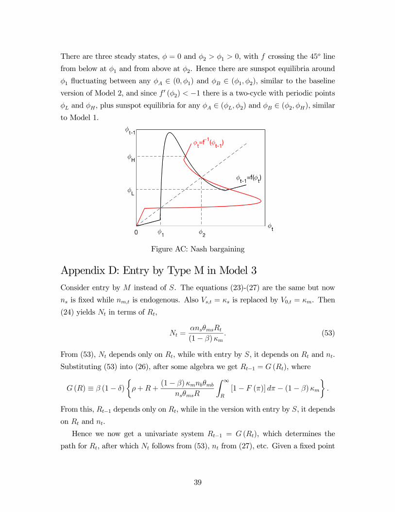
There are three steady states, = 0 and 2 1 0, with crossing the 45 line

from below at 1 and from above at 2. Hence there are sunspot equilibria around

1 fluctuating between any ∈ (0 1) and ∈ (1 2), similar to the baselineversion of Model 2, and since 0 (2) −1 there is a two-cycle with periodic points and , plus sunspot equilibria for any ∈ ( 2) and ∈ (2 ), similarto Model 1.

Figure AC: Nash bargaining

Appendix D: Entry by Type M in Model 3

Consider entry by instead of . The equations (23)-(27) are the same but now

is fixed while is endogenous. Also = is replaced by 0 = . Then

(24) yields in terms of ,

=

(1− ) (53)

From (53), depends only on , while with entry by , it depends on and .

Substituting (53) into (26), after some algebra we get −1 = (), where

() ≡ (1− )

½++

(1− )

Z ∞

[1− ()] − (1− )

¾

From this, −1 depends only on , while in the version with entry by , it depends

on and .

Hence we now get a univariate system −1 = (), which determines the

path for , after which follows from (53), from (27), etc. Given a fixed point

39

= (),

= (1− )

=

(1− )− −

= (1− ) [− ( + ) (1− )]

+ (1− ) [ () + ] (1− )

To guarantee the fixed point is a steady state we must check ≥ 0, both ofwhich hold iff ≥ ≡ ( + ) (1− ) (we also need ≤ but that

never binds). Hence, a solution to = () ≥ is a steady state with type

active; otherwise, there is no intermediation.

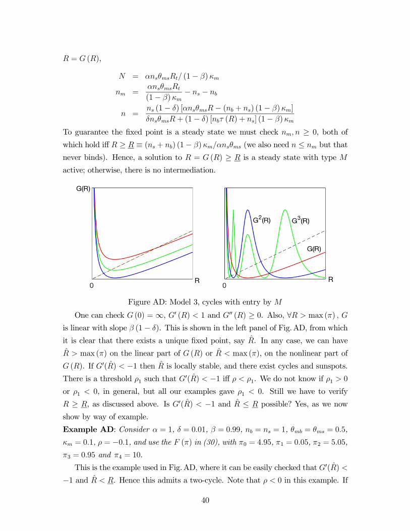
Figure AD: Model 3, cycles with entry by

One can check (0) =∞, 0 () 1 and 00 () ≥ 0. Also, ∀ max ()

is linear with slope (1− ). This is shown in the left panel of Fig.AD, from which

it is clear that there exists a unique fixed point, say . In any case, we can have

max () on the linear part of () or max (), on the nonlinear part of

(). If 0() −1 then is locally stable, and there exist cycles and sunspots.

There is a threshold 1 such that 0() −1 iff 1. We do not know if 1 0

or 1 0, in general, but all our examples gave 1 0. Still we have to verify

≥ , as discussed above. Is 0() −1 and ≤ possible? Yes, as we now

show by way of example.

Example AD: Consider = 1, = 001, = 099, = = 1, = = 05,

= 01, = −01, and use the () in (30), with 0 = 495, 1 = 005, 2 = 505,3 = 095 and 4 = 10.

This is the example used in Fig.AD, where it can be easily checked that 0()

−1 and . Hence this admits a two-cycle. Note that 0 in this example. If

40

we lower a little more, we can get higher-order cycles and chaotic dynamics. This

is shown in the right panel of Fig.AD, where we plot 3 () and see that there exist

fixed points other than , namely a pair of three cycles. Hence, we can explicitly

construct higher order cycles. Finally, one more result is that 0 implies and

must trade for some , Pr ( ) 0, if is in the market — just like in the

other version, a buy-and-hold-forever strategy is never a good idea at 0.

41

References

[1] G. Akerlof and R. Shiller (2009) Animal Spirits: How Human Psychology Drives

the Economy, and Why It Matters for Global Capitalism.

[2] D. Andolfatto and F. Martin (2013) “Information Disclosure and Exchange

Media,” RED 16, 527-539.

[3] D. Andolfatto, A. Berentsen and F. Martin (2019) “Money, Banking and Fi-

nancial Markets,” mimeo.

[4] D. Andolfatto, A. Berentsen and C. Waller (2014) “Optimal Disclosure Policy

and Undue Diligence,” JET 149, 128-152.

[5] C. Azariadis (1981) “Self-Fulfilling Prophecies,” JET 25, 380-396.

[6] C. Azariadis (1993) Intertemporal Macroeconomics.

[7] C. Azariadis and R. Guesnerie (1986) “Sunspots and Cycles,” RES 53, 725-737.

[8] J. Bhattacharya, J. Haslag and A. Martin (2005) “Heterogeneity, Redistribution

and the Friedman Rule,” IER 46, 437-454.

[9] B. Biais, T. Mariotti, G. Plantin and J. Rochet (2007) “Dynamic Security

Design: Convergence to Continuous Time and Asset Pricing Implications,”

RES 74, 345-90.

[10] V. Bencivenga and B. Smith (1991) “Financial Intermediation and Endogenous

Growth,” RES 58, 195-209.

[11] A. Berentsen, G. Camera and C. Waller (2007) “Money, Credit, and Banking,”

JET 135, 171-195.

[12] J. Boyd and E. Prescott (1986) “Financial Intermediary-Coalitions,” JET 38,

211-232.

[13] K. Burdett and M. Coles (1997) “Marriage and Class,” QJE 112, 141-168.

[14] C. Calomiris and S. Haber (2014) Fragile by Design: The Political Origins of

Banking Crises and Scarce Credit.

[15] R. Cavalcanti, A. Erosa and T. Temzilides (1999) “Private Money and Reserve

Management in a Random-Matching Model,” JPE 107, 929-945.

[16] R. Cavalcanti and N. Wallace (1999) “A Model of Private Banknote Issue,”

RED 2, 104-136.

[17] R. Cavalcanti and N.Wallace (1999) “Inside and Outside Money as Alternative

Media of Exchange,” JMCB 31, 443-457.

42

[18] B. Champ, B. Smith and S. Williamson (1996) “Currency Elasticity and Bank-

ing Panics: Theory and Evidence,” CJE 29, 828-864.

[19] V. Chari and R. Jagannathan (1988) “ Banking Panics, Information, and Ra-

tional Expectations Equilibrium,” JF 43, 749-761.

[20] R. Clower (1965) “A Reconsideration of the Microfoundations of Monetary

Economics,” Western Econ Journal 6, 1-8.

[21] C. Comerton-Forde, T. Hendershott, C. Jones, P. Moulton and M. Seasholes

(2010) “Time Variation in Liquidity: The Role of Market-Maker Inventories

and Revenues,” JF 65, 295-331.

[22] T. Dang, G. Gorton, B. Holmström and G. Ordonez (2017) “Banks as Secret

Keepers,” AER 107, 1005-1029.

[23] G. Debreu (1959) Theory of Value.

[24] D. Diamond (1984) “Financial Intermediation and Delegated Monitoring,”RES

51, 393-414.

[25] D. Duffie, N. Gârleanu and L. Pederson (2005) “Over-the-Counter Markets,”

Econometrica 73, 1815-1847.

[26] P. DeMarzo and M. Fishman (2007) “Agency and Optimal Investment Dynam-

ics,” RFS 20, 151-188.

[27] X. Freixas and J. Rochet (2008) Microeconomics of Banking.

[28] M. Friedman (1960) A Program for Monetary Stability.

[29] M. Friedman and A. Schwartz (1963) A Monetary History of the United States,

1867-1960.

[30] G. Gorton and G. Pennacchi (1990) “Financial Intermediaries and Liquidity

Creation,” JF 45, 49-71.

[31] G. Gorton and A. Winton (2003) “Financial Intermediation,” in G. Constanti-

nides, M. Harris, R. Stulz, eds. Handbook of the Economics of Finance.

[32] C. Gu (2011) “Herding and Bank Runs,” JET 146, 163-188.

[33] C. Gu, F. Mattesini, C. Monnet and R. Wright (2013) “Banking: A New

Monetarist Approach,” RES 80, 636-662.

[34] C. Gu, F. Mattesini, C. Monnet and R. Wright (2013) “Endogenous Credit

Cycles,” JPE 121, 940-965.

43

[35] C. Gu, F. Mattesini and R. Wright (2016) “Money and Credit Redux,” Econo-

metrica 84, 1-32.

[36] C. Gu and R. Wright (2016) “Monetary Mechanisms,” JET 163, 644-657.

[37] T. Hu and G. Rocheteau (2015) “Monetary Policy and Asset Prices: A Mech-

anism Design Approach,” JMCB 47, 39-76.

[38] A. Huang (2017) “On the Number and Size of Banks,” mimeo.

[39] E. Kalai (1977) “Proportional Solutions to Bargaining Situations: Interpersonal

Utility Comparisons,” Econometrica 45, 1623-1630.

[40] T. Kehoe and D. Levine (1993) “Debt-Constrained Asset Markets,” RES 60,

865-888.

[41] J. Keynes (1936) The General Theory of Employment, Interest and Money.

[42] C. Kindleberger (1978) Manias, Panics and Crashes.

[43] N. Kiyotaki and R. Wright (1989) “On Money as a Medium of Exchange,” JPE

97, 927-954.

[44] N. Kocherlakota (1998) “Money is Memory,” JET 81, 232-251.

[45] J. Lacker (2015) “From Country Banks to SIFIs: The 100-year Quest for Fi-

nancial Stability,” speech at Louisiana State University.

[46] R. Lagos and G. Rocheteau (2009) “Liquidity in Asset Markets with Search

Frictions,” Econometrica 77, 403-426.

[47] R. Lagos, G. Rocheteau and R. Wright (2017) “Liquidity: A New Monetarist

Perspective,” JEL 55, 371-440.

[48] R. Lagos and R. Wright (2005) “A Unified Framework for Monetary Theory

and Policy Analysis,” JPE 113, 463-484.

[49] R. Lagos and S. Zhang (2019) “Turnover Liquidity and the Transmission of

Monetary Policy,” AER, forthcoming.

[50] H. Leland and D. Pyle (1977) “Informational Asymmetries, Financial Structure,

and Financial Intermediation,” JF 32, 371-387.

[51] B. Lester, A. Postlewaite and R. Wright (2012) “Liquidity, Information, Asset

Prices and Monetary Policy,” RES 79, 1209-38.

[52] Y. Li, G. Rocheteau and P. Weill (2012) “Liquidity and the Threat of Fraudu-

lent Assets,” JPE 120, 815-46.

44

[53] M. Loberto (2017) “Safety Traps, Liquidity and Information-Sensitive Assets,”

mimeo.

[54] H. Minsky (1992) “The Financial Instability Hypothesis,” Levy Economics In-

stitute WP 74.

[55] C. Monnet and E. Quintin (2017) “Rational Opacity,” RFS 30, 4317-4348.

[56] E. Nosal, Y. Wong and R. Wright (2019) “Intermediation in Markets for Goods

and Markets for Assets,” mimeo.

[57] J. Peck and K. Shell (2004) “Equilibrium Bank Runs,” JPE 111, 103-123.

[58] J. Peck and A. Setayesh (2019) “A Diamond-Dybvig Model in which the Level

of Deposits is Endogenous,” mimeo.

[59] C. Pissarides (2000) Equilibrium Unemployment Theory.

[60] S. Quinn (1997) “Goldsmith-Banking: Mutual Acceptance and Interbanker

Clearing in Restoration London,” Explorations Econ History 34, 411-442.

[61] R. Rajan (2005) “Has Financial Development Made the World Riskier?” Pro-

ceedings of the Jackson Hole Conference, 313-369.

[62] G. Rocheteau and E. Nosal (2017) Money, Payments and Liquidity, 2nd ed.

[63] G. Rocheteau and A. Rodriguez-Lopez (2014) “Liquidity provision, interest

rates, and unemployment,” JME 65, 80-101.

[64] R. Rogerson (1988) “Indivisible Labor, Lotteries and Equilibrium,” JME 21,

3-16

[65] A. Rolnick and W. Weber (1986) “Inherent Instability in Banking: The Free

Banking Experience,” Cato Journal 5, 877-890.

[66] A. Rubinstein and A. Wolinsky (1987) “Middlemen,” QJE 102, 581-94.

[67] D. Sanches and S. Williamson (2010) “Money and Credit with Limited Com-

mitment and Theft,” JET 145, 1525-49.

[68] F. Sanello (2003) The Knights Templars: God’s Warriors, the Devil’s Bankers.

[69] G. Selgin (2018) “Banks,” Encyclopedia Britannica, https://www.britannica.

com/topic/bank.

[70] K. Shell (1992) “Sunspot Equilibria,” New Palgrave Dictionary of Money and

Finance.

45

[71] S. Shi (2009) “Directed Search for Equilibrium Wage-Tenure Contracts,”

Econometrica 77, 561-584.

[72] A. Shleifer and R. Vishny (2010) “Unstable Banking,” JFE 97, 306-318.

[73] B. Smith (2002) “Monetary Policy, Banking Crises, and the Friedman Rule,”

AER 92, 128-134.

[74] X. Vives (2016) Competition and Stability in Banking: The Role of Regulation

and Competition Policy.

[75] P. Weill (2007) “Leaning against the Wind,” RES 74, 1329-1314.

[76] N. Williams (2015) “Financial Instability via Adaptive Learning,” mimeo.

[77] R. Wright (2017)“On the Future of Macro: A New Monetarist Perspective,”

Oxford Rev Econ Policy 34 (2018), 107-131.

46