Embed Size (px)
Citation preview

810
On the initialization of Tropical Cyclones
M. Bonavita, M. Dahoui, P. Lopez, F. Prates, E. Hólm, G. De Chiara,
A. Geer, L. Isaksen, B. Ingleby
Research Department
September 2017

Series: ECMWF Technical Memoranda A full list of ECMWF Publications can be found on our web site under: http://www.ecmwf.int/publications/ Contact: [email protected] © Copyright 2017 European Centre for Medium Range Weather Forecasts Shinfield Park, Reading, Berkshire RG2 9AX, England Literary and scientific copyrights belong to ECMWF and are reserved in all countries. This publication is not to be reprinted or translated in whole or in part without the written permission of the Director General. Appropriate non-commercial use will normally be granted under the condition that reference is made to ECMWF. The information within this publication is given in good faith and considered to be true, but ECMWF accepts no liability for error, omission and for loss or damage arising from its use.

On the initialization of Tropical Cyclones
Technical Memorandum No.810 1
Table of Contents
1 Introduction ..................................................................................................................................... 1
2 Algorithmic Aspects ........................................................................................................................ 5
3 The role of dropsondes in TC analysis ............................................................................................ 7
4 Robust Quality Control of Dropsonde Observations ..................................................................... 12
4.1 An adaptive First Guess Quality Control algorithm .............................................................. 14
4.2 Experimental results .............................................................................................................. 19
5 Multi-eyed cyclones and non-Gaussian priors .............................................................................. 23
5.1 Symptoms .............................................................................................................................. 23
5.2 Therapies ............................................................................................................................... 27
6 Verification of Tropical Cyclones analyses and forecasts............................................................. 30
7 Discussion and research perspectives ............................................................................................ 32
8 Conclusions ................................................................................................................................... 35
Abstract
Recent increases in the IFS model resolution have improved its ability to produce realistic forecasts
of tropical cyclones but they also present new challenges to the data assimilation system. This is
because standard assumptions made in 4D-Var are called into question when the data assimilation
system has to deal with observations sampling the extreme conditions, both actual and forecasted,
around a tropical cyclone centre. We present here examples of these problems as encountered in the
operational ECMWF analysis and the solutions adopted to correct them. These include introducing an
adaptive quality control algorithm for dropsonde observations, the reduction of the resolution of the
EDA-derived background errors used in 4D-Var together with a non-homogeneous noise filtering
technique. These investigations have also highlighted a number of promising avenues of further
research, which have the potential to improve both the initialisation of tropical cyclones and the global
accuracy of the ECMWF analyses and forecasts.
1 Introduction
Tropical cyclones (TC) are some of the most damaging weather events, even today causing significant
number of casualties and widespread damage to property (Doocy et al., 2013) through a combination of
destructive winds, torrential rains, flooding and storm surges. The ability to provide detailed, timely and
accurate numerical weather prediction (NWP) guidance to the operational forecasting centres tasked
with issuing the relevant alerts and warnings is thus a fundamental aspect of the mitigation effort.

On the initialization of Tropical Cyclones
2 Technical Memorandum No.810
During the past 25 years, the skill of tropical cyclone forecasts has steadily increased at ECMWF and
in all other global NWP centres, more markedly for cyclone tracks (Yamaguchi et al., 2017). These
advances have been the combined result of developments in the prognostic model, increased resolution,
better observational coverage and advances in data assimilation methods. This combination of factors
has led to a general improvement of all aspects of the forecast, and the improvements seen in TC
forecasts can be seen as a consequence of this wider trend. It is important to note in this context that,
differently from other global NWP Centres (Kleist, 2011; Heming, 2016), ECMWF does not use pseudo-
observations of the TC central pressure or the TC position (sometimes known as TC Vitals: Trahan and
Sparling, 2012) either directly or through a dynamical relocation of the vortex.
The recent upgrades in horizontal resolution of the ECMWF atmospheric model (currently approx. 9
km grid-spacing for the deterministic high resolution atmospheric model (HRES); 18 km for the
Ensemble of Data Assimilation, EDA, and the ensemble forecasts, ENS) have resulted in an increased
realism of the simulated structure and intensity of tropical cyclones (Holm et al, 2015; Mogensen et al.,
2017). While this implies that background forecasts of tropical cyclones tend to show more realistic
structures and depth, relatively small discrepancies between the background and actual TC location can
produce very large observation-background departures (O-B). These large departures, in turn, present
the analysis algorithm with difficult choices in terms of observation quality control and, as discussed in
the following, they test the limits of applicability of incremental 4D-Var. We note that analogous
problems have been encountered and discussed in the EnKF framework (Chen and Snyder, 2007; Torn
and Hakim, 2009; Torn, 2010), where it has been shown, for example, that assimilating vortex position
information in cases where expected vs actual positions differed more than the vortex size can lead to
negative effects on the analysis quality.
An example of these problems is shown in Fig. 1. In the left panel the temporal evolution of the analysed
minimum mean sea level pressure (min MSLP) of the operational EDA control (unperturbed) member
of the ECMWF Integrated Forecasting System (IFS) Cycle 41r2 is shown (continuous line), while the
estimated min MSLP from the official advisories is shown as red dots. The right panel shows the
temperature analysis increments of EDA member 14 valid on 2015-10-02 at 09 UTC, at the end of the
first outer loop iteration (unsurprisingly, the minimization failed to converge due to numerical
instabilities in the second outer loop iteration).
Figure 1. Left panel: time evolution of the analysed minimum mean sea level pressure for the EDA
control member (continuous line) and of the estimated minimum sea level pressure of Hurricane Joaquin

On the initialization of Tropical Cyclones
Technical Memorandum No.810 3
according to official advisories (units: hPa). Right panel: temperature analysis increments at model
level 120 (approx. 900 hPa) for EDA member 14, valid on 2015-10-02 at 09 UTC (red positive, green-
blue negative; units: Kelvin).
The difficulties encountered by the analysis algorithm were found to be connected to the very large O-
B departures of the dropsonde winds entering the assimilation cycle (Fig. 2, left panel: wind vector
observation departures with respect to the background forecast for the 2015-10-02 00UTC analysis;
right panel: wind vector observation departures with respect to the analysed wind field). It is apparent
that dropsonde wind observations in the vicinity of the centre of the tropical cyclone can present
departures well in excess of 50 m/s with respect to the background forecast (In this specific case
observation-background departures of up to 70 m/s were registered). A sensitivity experiment
blacklisting dropsonde wind observations prevented the numerical failures in the variational analysis
that occurred for some of the EDA members and provided a more regular time evolution of the analysed
cyclone. However, the depth and strength of the cyclone were then consistently under-estimated (Fig.
3).
Figure 2. Left panel: Observation-background departures from the background forecast of dropsonde
wind vectors active in the 2015-10-02 00UTC analysis in the 600-1013 hPa atmospheric layer (coloured
dots, see legend; units: m/s); black triangle denote estimated position of tropical cyclone Joaquin at
nominal analysis time); MSLP background forecast valid at nominal analysis time (black isolines, 5hPa
intervals). Right panel: As left panel but for the corresponding analysed fields.

On the initialization of Tropical Cyclones
4 Technical Memorandum No.810
Figure 3. Time evolution of the analysed minimum mean sea level pressure for the EDA control member
(red continuous line); EDA control member with blacklisted dropsonde wind observations (green
continuous line); and of the estimated minimum sea level pressure of Hurricane Joaquin according to
official advisories (units: hPa).
A distinct problem in the initialization of tropical cyclones was also highlighted in conjunction with the
pre-operational tests leading to the horizontal resolution upgrade of the IFS in 2016 (from approx. 18
km grid spacing to approx. 9 km). A typical example is shown in Figure 4 where the mean sea level
pressure field from the pre-operational analysis valid on 2015-10-23, 12UTC (Cycle 41r1; TL1279
resolution) is presented in the left panel and the corresponding analysis for the higher resolution
experimental cycle 41r2 (TCo1279 resolution) is presented in the right panel. The red triangle in the
plots denotes the estimated position of Hurricane Patricia, whose minimum mean sea level (MSL)
pressure was also estimated by the official advisories to have reached 880 hPa at the time of the analysis.
It is evident that both analyses are very far from producing a realistic description of the intensity of this
tropical cyclone. In addition, the higher resolution analysis produces a “double-eyed” configuration of
the cyclone, with two separate MSL minima around the reported position. This “multi-eyed” type of
behaviour more often occurred for tropical cyclones that were poorly constrained by observations, either
conventional observations (SHIPS, BUOYS, Dropsondes) and/or scatterometer observations.

On the initialization of Tropical Cyclones
Technical Memorandum No.810 5
Figure 4. Left panel: Analysed mean sea level pressure for the operational IFS cycle (41r1) valid on
2015-10-23, 12 UTC. Right panel: As left panel, for IFS cycle 41r2. The red triangle denotes the
estimated position of Hurricane Patricia at the analysis time.
In this paper, we discuss in more detail the behaviour of the ECMWF assimilation system with respect
to tropical cyclone initialization in light of the issues described above and the solutions adopted to
improve the accuracy and robustness of the operational analysis. In Sect. 2 we examine some of the
algorithmic constraints which can affect the behaviour of the ECMWF data assimilation system in the
presence of large discrepancies between observations and model background forecast. In Sect. 3 some
aspects of the current use and deployment practices of dropsondes launched in the vicinity of tropical
cyclones are reviewed and a representative example is analysed in detail. In Sect. 4 we discuss the
changes introduced in a recent IFS cycle (Cycle 43r3, operational from July 2017) to deal with some of
the problems highlighted in connection with the use of dropsonde observations. The impact of these
changes on analysis performance is illustrated in terms of representative test cases and more
comprehensive performance statistics. In Sect. 5 we proceed to discuss the issues connected with the
appearance of “multi-eyed” tropical cyclones in the ECMWF analyses and what has been done to tackle
this problem in recent IFS cycles. Measuring progress in tropical cyclone initialisation and prediction
requires accurate verification data, which is still difficult to obtain, as direct observations of the relevant
TC quantities are infrequent. In Sect. 6 we discuss some of the issues connected with TC verification
and some new recent diagnostic tools introduced at ECMWF. Producing more accurate and reliable
analyses and forecasts of Tropical Cyclones will still require efforts in terms of data assimilation
methodology, improved observation usage and model development: the more interesting lines of current
and near future research, from the ECMWF perspective, are discussed in Sect. 7. Conclusions are drawn
in Sect. 8.
2 Algorithmic Aspects
To understand the issues facing the 4D-Var analysis in the presence of large O-B departures let us
consider the standard strong constraint 4D-Var cost function:
𝐽(𝐱0) =1
2(𝐱0 − 𝐱𝑏)T𝐏𝑏
−1(𝐱0 − 𝐱𝑏) +1
2∑(𝐲𝑘 − 𝐺𝑘(𝐱0))
T𝐑𝑘
−1(𝐲𝑘 − 𝐺𝑘(𝐱0))
𝐾
𝑘=0
(1)
Where 𝐱0 is the control vector at the start of the assimilation window; 𝐱𝑏and 𝐏𝑏 are the background and
its expected error covariance matrix; 𝐲𝑘 and 𝐑𝑘 are the set of observations presented to the analysis in
the k sub-window and their expected error covariances; and 𝐺𝑘 is a generalised observation operator that
produces the model equivalents of 𝐲𝑘 by integrating the model from t0 to tk and then applying the
standard observation operator 𝐻𝑘 to the propagated fields, i.e.:
𝐺𝑘 = 𝐻𝑘°𝑀𝑡0→𝑡𝑘 (2)
Incremental 4D-Var (Courtier et al., 1994) approximates the minimization of the non-linear cost
function (1) as a sequence of minimizations of linear, quadratic cost functions defined in terms of
perturbations around a sequence of progressively more accurate trajectories (i.e., non-linear model
integrations). The cost function linearised around a trajectory 𝐱𝑡 can be expressed as an exact quadratic
problem in terms of the initial time increment δ𝐱0:

On the initialization of Tropical Cyclones
6 Technical Memorandum No.810
𝐽(δ𝐱0) =1
2(𝛿𝐱0 + 𝐱0
𝑡 − 𝐱𝑏)T𝐏𝑏−1(𝛿𝐱0 + 𝐱0
𝑡 − 𝐱𝑏)
+1
2∑(𝐝𝑘 − 𝐆𝑘(δ𝐱0))
T𝐑𝑘
−1(𝐝𝑘 − 𝐆𝑘(δ𝐱0))
𝐾
𝑘=0
(3)
Where 𝐝𝑘 = 𝐲𝑘 − 𝐺𝑘(𝐱0𝑡 ) are the observation departures around the latest model trajectory and 𝐆𝑘 =
𝐇𝑘𝐌𝑡0→𝑡𝑘 is the linearisation of the generalised observation operator.
In the observation part of the cost function, the so-called “tangent linear approximation” has been made
in going from (1) to (3):
𝐲𝑘 − 𝐺𝑘(𝐱0) = 𝐲𝑘 − 𝐺𝑘(𝐱0𝑡 + δ𝐱0)
= 𝐲𝑘 − 𝐺𝑘(𝐱0𝑡 ) − 𝐆𝑘(δ𝐱0) −
1
2 (δ𝐱0)T (
∂𝐆𝑘
∂𝐱)
𝐱𝑡(δ𝐱0) − 𝑂(‖δ𝐱0‖3)
≈ 𝐲𝑘 − 𝐺𝑘(𝐱0𝑡 ) − 𝐆𝑘(δ𝐱0) (4)
In the Taylor expansion in Eq. (4), terms of O(‖δ𝐱0‖2) and higher are neglected. This is justified if
either the dependence of the linearization of 𝐺𝑘 (i.e., 𝐆𝑘 = 𝐇𝑘𝐌𝑡0→𝑡𝑘) to the reference trajectory is
negligible or the increments δ𝐱0 are in some sense small. Concerning the first aspect, experience has
shown that there is a clear sensitivity of both the linearised observation operator and the linearised model
to the linearisation state (e.g., Bauer et al., 2010; Janisková, M., and P. Lopez, 2013).
The size of the increments δ𝐱0 can be estimated from linear Kalman Filter theory as:
δ𝐱0 ≈ 𝐏𝑏𝐇𝑇(𝐇𝐏𝑏𝐇𝑇 + 𝐑)−1𝐝𝑘 (5)
The size of the increments is thus, to a first approximation, a linear function of the observation
departures. Larger observation departures will thus make the tangent linear hypothesis progressively
less valid. Note how larger assumed background errors will also produce bigger increments, especially
when they are of comparable magnitude to assumed observation errors. In this regard, the introduction
of the Ensemble of Data Assimilations (EDA, Isaksen et al., 2010) in the ECMWF analysis algorithm
to estimate flow-dependent background errors, has led to a sizable increase in the magnitude of estimated
background errors in the vicinity of active weather systems in general and tropical cyclones in particular
(e.g., Bonavita et al., 2012; Holm et al., 2015). On the other hand, we see from Eq. (5) that bigger
expected observation errors tend to reduce the size of the increments during the variational minimization
process and thus keep the system within the bounds of validity of the tangent linear assumption.
Large O-B departures can also can also test the resilience of the algorithms used in the Quality Control
(QC) of the observations. The observation QC algorithms used in the ECMWF data assimilation cycle
are of two types.
First, a background QC check is applied to the magnitude of the O-B departures:
(y𝑘 − 𝐺𝑘(𝐱0𝑏))
2< 𝑍𝑅𝐸𝐽 ∗ (𝜎𝑜
2 + 𝜎𝑏2)
2 (6)
where 𝜎𝑜2 is assumed observation error variance and 𝜎𝑏
2 is the background error variance interpolated to
the observation location. ZREJ is a pre-specified rejection limit that is typically in the 9-25 range. This
means that observations are completely rejected and play no further role in the assimilation if the
magnitude of their departures are between 3 to 5 times the magnitude of their expected total errors,
assuming uncorrelated observation and background errors. In the case of dropsonde observations the

On the initialization of Tropical Cyclones
Technical Memorandum No.810 7
rejection limit is further relaxed to 100, so that departures need to exceed 10 times their expected values
to be rejected. Taking into account that background errors estimated from the EDA background standard
deviation can easily exceed 6-7 m/s for each wind component in the vicinity of tropical cyclones, it is
clear that this quality control step will allow most of the dropsonde observations into the analysis. It is
interesting to note that the use of more realistic values of background errors near tropical cyclones affects
the analysis in two ways: a) it increases the magnitude of the 4D-Var increments and b) it allows
observation with larger O-B departures into the analysis. These effects together tend to produce even
larger increments in the analysis.
An additional QC step is performed inside the 4D-Var analysis, and it is thus commonly referred to as
variational QC (VarQC). In the ECMWF implementation (Tavolato and Isaksen, 2015), the standard
Gaussian assumption for the statistical distribution of the observation errors is changed to a Huber norm
distribution (Huber, 1964), which is Gaussian in the centre but has exponential tails beyond some
predefined transition points. The use of the Huber norm allows 4D-Var to perform a “soft” QC on
observations with large departures, by effectively reducing their impact on the final analysis, but not
discarding them completely. We note however that in its current ECMWF implementation the Huber
norm VarQC is not active during the first outer loop minimization. As the first minimization is the one
that produces the biggest increments in the analysis, marginal observations with large O-B departures
can still have a large effect on the final analysis even when the VarQC has effectively rejected them in
successive outer loops. It is also interesting to note that the implementation of the Huber norm requires
the identification of the transition points (left and right) where the distribution transforms from Gaussian
to exponential. As shown in Tavolato and Isaksen, 2015, this requires a careful statistical analysis of
large samples of O-B departures for the specified observation type. It is clearly difficult to construct
representative samples for infrequent observations such as dropsondes and comparison with radiosonde
O-B statistics is complicated by the sampling of dropsondes (usually near TCs).
3 The role of dropsondes in TC analysis
Most TC dropsondes are provided by the USA for storms approaching North America or Hawaii.
Several different types of aircraft are used to launch the dropsondes. The US Air Force uses WC-130
Hercules aircraft at low or medium altitudes up to 3 km (10000 feet, see
http://www.hurricanehunters.com/plane.html), NOAA uses Gulfstream-IV (high altitude), and P-3 (low
or medium altitude) aircraft (Aberson et al, 2010; these aircraft carry various additional instruments but
the data are not currently available over the GTS7). In recent years, NOAA and NASA have also used
the autonomous Global Hawk aircraft (at altitudes up to 22 km,
https://www.esrl.noaa.gov/psd/psd2/coastal/satres/ghawk_dropsonde.html). Several different
flight/release patterns are possible, but from an assimilation point of view, the main distinction is
between eyewall/eye sampling (which is mainly from the aircraft flying at about 700 hPa) and more
general sampling of the storm environment. Even with relatively high resolution global NWP systems
eyewall observations pose severe problems of representativeness errors - discussed further below. In
the Asia-Pacific region, there was a 2008 field experiment (Weissmann et al, 2011). Taiwan operates
the ongoing DOTSTAR program (http://typhoon.as.ntu.edu.tw/DOTSTAR/en/), and apparently, Hong
Kong has TC dropsonde capability, but there are relatively few reports from this region.
In the current ECMWF IFS dropsonde observations are treated similarly to radiosonde observations,
with the same default expected observation error standard deviations (based on Ingleby, 2017, there has

On the initialization of Tropical Cyclones
8 Technical Memorandum No.810
been a change to reduce the specified temperature and humidity errors for certain radiosonde types, this
does not affect the values specified for dropsondes). In recent years, a growing number of radiosonde
reports are becoming available in binary BUFR format (Ingleby et al., 2016), which allows the
transmission of the exact position of the sonde during the ascent. Being able to account for radiosonde
drift in the horizontal has been shown to be beneficial to the O-B statistics (Ingleby and Edwards, 2015).
This is still not possible for dropsonde observations, although it is hoped that high-resolution reports
with positions at each level will become available over the Global Telecommunication System (GTS)
in 2018.
The current practice of treating dropsonde profiles as vertical and instantaneous is particularly
problematic for eyewall reports. Different drop patterns are illustrated in Fig. 5, where the O-B
departures of dropsonde wind vectors are shown for a 12-hour assimilation window during the lifetime
of hurricane Sandy (left panel) and of hurricane Matthew (right panel). While both hurricanes’
environment is sampled by a long-range, approx. circular deployment of dropsondes, the hurricane
structure itself is sampled very differently. In Sandy’s case, a distribution of dropsondes on an irregular
grid around the hurricane core is visible; in the more recent Matthew case the dropsondes are clustered
together near the hurricane’s core. The differences are partly because Sandy had a less well-defined
eyewall and partly because of the altitude of the reconnaissance flights (Aberson, pers. comm., 2017).
Figure 5. Left panel: O-B departures of dropsonde wind vector observations active in the 2012-10-26
00UTC analysis in the 600-1013 hPa atmospheric layer (coloured dots, see legend; units: m/s; black
triangle denote estimated position of hurricane Sandy at nominal analysis time); MSLP background
forecast valid at nominal analysis time (black isolines, 5hPa intervals). Right panel: As left panel for
the 2016-10-04 00UTC analysis of hurricane Matthew.
To see in more detail the possible consequences of eyewall reports on the TC initialization, let us
consider the case of hurricane Matthew in more detail. Hurricane Matthew (Fig. 6, left panel) was a
major category 5 tropical cyclone in the 2016 Atlantic hurricane season, which brought devastation to
large swaths of the Caribbean islands and the south eastern USA (Stewart, 2017). The ECMWF
operational analysis valid at 12 UTC on 2016-10-01 assimilated observations from five dropsondes
deployed in a 1-hour period around the nominal analysis time near the TC core (Fig. 6, right panel).
Looking at the observed wind components during the dropsonde descent (Fig. 7), it is apparent that some
of the dropsondes were caught in the strong axisymmetric flow around the TC core. This effect is evident
for dropsonde 3 whose observed wind observations are shown in the left panel of Figure 8: during its

On the initialization of Tropical Cyclones
Technical Memorandum No.810 9
descent from approx. 700 hPa down to the surface, the sonde is swept around the TC core for about a
quarter of its angular circumference. This is consistent with the initial distance of the dropsonde to the
reported TC position (approx. 12 km), typical fall speeds of 12-15 m/s and reported horizontal wind
speeds in the 50 to 67 m/s range.
Figure 6. Left panel: Image of Hurricane Matthew derived from the MODIS sensor L1B radiances on
board the NASA Terra sun-synchronous satellite on 2016-10-01, 15 UTC (credits: https://modis-
atmos.gsfc.nasa.gov/index.html). Right panel: Estimated position of Hurricane Matthew on 2016-10-
01, 12 UTC (black triangle) and launch position of dropsondes near Hurricane Matthew core from
11.53 UTC to 12.49 UTC on 2016-10-01 (coloured circles).The estimated position of Hurricane
Matthew and the launch position of dropsonde 1 (blue circle) overlap.
Figure 7. Left panel: observed zonal wind components for dropsonde observations near the core of
hurricane Matthew from 11.53 UTC to 12.49 UTC on 2016-10-01 (colour code as in Fig. 6, right panel;
units: m/s), as a function of reported pressure (units: hPa). Right panel: as left panel for the meridional
wind components.
An immediate effect of not being able to take the horizontal drift of the dropsonde into account is shown
in the right panel of Figure 8, where the vertical profile of the root mean squared observation departures
of the wind vector for dropsonde 3 is shown. These departures are seen to increase during the sonde

On the initialization of Tropical Cyclones
10 Technical Memorandum No.810
descent as the wind observations are compared to background fields that are less and less representative
of the local flow. This inconsistency appears to have a significant effect on the resulting analysed TC
structure. In Figure 9, top row, we show the background forecast (left panel) and the corresponding
analysis (right panel) of the ECMWF operational cycle for the equivalent potential temperature field at
850 hPa, together with the wind vector observation departures produced by dropsonde 3 (black arrows;
magnitude of wind vector departures ranges from 60 to 95 m/s). These large wind departures across a
temperature field with sharp spatial gradients tend to disrupt the TC axisymmetric thermal structure
towards a frontal-type configuration. However, the ensuing forecast of the TC tends to return rapidly (in
about 3-6 hours) to a more axisymmetric structure (Fig. 9, bottom row), suggesting that the solution
produced by the analysis was not dynamically consistent.
Figure 8. Left panel: observed wind vectors for dropsonde 3 launched at 12.45 UTC on 2016-10-01
(numbers in the legend indicate reported height of wind measurement in hPa; length of wind arrows in
the legend is 20 m/s); Right panel: profile of RMS wind vector observation departures for dropsonde 3
as a function of reported pressure (units: hPa, m/s).

On the initialization of Tropical Cyclones
Technical Memorandum No.810 11
Figure 9. Left panel, top: Observation departures (O-B) for dropsonde 3 winds (black arrows) and
operational background forecast of equivalent potential temperature at 850 hPa valid on 2016-10-01
at 12UTC. Right panel, top: as left panel, for the operational analysis valid on 2016-10-01 at 12UTC.
Left panel, bottom: t+3h forecast of equivalent potential temperature at 850 hPa started from
operational analysis valid on 2016-10-01 at 12UTC. Right panel, bottom: as left panel, for t+6h forecast
(units: Kelvin).
Another significant side effect of the presence of the very large O-B departures caused by eyewall
dropsondes is visible in the EDA-estimated background errors. As shown in Fig 10, these errors tend to
show complex, multi-modal structures as a result of both EDA members location becoming more
spatially scattered around the TC core and also because some of the members develop multi-core
structures in their analyses and short-range forecasts. As these error estimates are then used in the
successive analysis update, the potential for negatively affecting the accuracy of TC estimation in the
data assimilation cycle is apparent.

On the initialization of Tropical Cyclones
12 Technical Memorandum No.810
Figure 10. Left panel: EDA-derived standard deviation of vorticity background errors for the
operational IFS valid on 2016-10-01 at 21 UTC (black triangle shows estimated position of TC Matthew
on 2016-10-21 at 18UTC). Right panel: Vorticity background forecast of member 4 of the operational
EDA valid on 2016-10-21 at 21 UTC. Units 10-5s-1.
4 Robust Quality Control of Dropsonde Observations
The examples discussed in Sections 1 and 3 have highlighted problems connected with the use of
dropsondes deployed close to the centre of a tropical cyclone in a high resolution, variational data
assimilation system. A straightforward solution would be to simply exclude dropsonde observations in
the vicinity of the TC centre. This solution was adopted in the operational IFS configuration from 7
October 2016, in order to respond to repeated failures in the convergence of the 4D-Var algorithm in
multiple members of the EDA system. These failures were tracked to the assimilation of dropsonde
measurements in the vicinity of TC Matthew. However, as already shown in the case of hurricane
Joaquin during the 2015 Atlantic hurricane season (Fig. 3), blacklisting dropsonde observations
generally solves the numerical failures in the minimization, but it also tends to reduce the depth of the
analysed TCs. This was also found to be the case for hurricane Matthew (Fig. 11).

On the initialization of Tropical Cyclones
Technical Memorandum No.810 13
Figure 11. Time evolution of the analysed minimum mean sea level pressure for the High Resolution
analysis of the 43r1 IFS cycle (green continuous line); High Resolution analysis with blacklisted
dropsonde observations near hurricane Matthew core (blue dashed line); estimated minimum sea level
pressure of Hurricane Matthew according to official advisories (red dots, units: hPa).
Another potential problem is the fact that the analysis system is not robust with respect to the presence
of dropsonde observations that might have eluded the observation screening. Figure 12 shows how a
single near core dropsonde that escaped blacklisting by the screening degraded the analysis of hurricane
Matthew (valid on 2016-10-01 12UTC).
Figure 12. Left panel: Observation-analysis departures of dropsonde wind vectors active in the 2016-
10-01 12UTC analysis update in the 600-1013 hPa atmospheric layer (coloured dots, see legend; units:
m/s) for the experiment with correct blacklisting of “eyewall” dropsondes; black triangle denote
estimated position of hurricane Matthew at nominal analysis time; MSLP analysis valid at nominal
analysis time (black isolines, 5hPa intervals). Right panel: As left panel for experiment in which one
“eyewall” dropsonde (purple dot) was accidentally allowed to enter the assimilation cycle.

On the initialization of Tropical Cyclones
14 Technical Memorandum No.810
Numerous other trials were also performed changing the rejection limits for the background QC check
on dropsonde observations as described in Sect. 2. Results (not shown) were generally unsatisfactory,
as it proved impossible to find rejection limits that gave consistently good performance.
4.1 An adaptive First Guess Quality Control algorithm
The examples discussed in the previous sections confirm that dropsonde wind observations are
important for producing analyses with realistic estimates of the depth and location of tropical cyclones.
However, the current quality control procedures based on selective blacklisting and first guess rejections
are possibly too blunt an instrument to deal with the complex task of deciding whether to retain an
observation with a large initial departure from the model background and how much weight it should
be given in the analysis update. An adaptive QC procedure should be able to take these decisions based
on information about the local flow and the a-priori estimates of the relevant error sources.
A common way to characterize the errors present in an observation y is through the decomposition
(Lorenc, 1986):
𝑦 = ℎ(𝒙) + 휀𝐼 + 휀𝑅 + 휀𝐻 (7)
where h is the observation (or forward model) operator linking the true model state x to the observation;
휀𝐼is the error due to the accuracy and precision of the instrument (Instrument error); 휀𝑅 is the
representativity error, which accounts for the variability of the observed quantities on scales not resolved
by the model sate; 휀𝐻 is the forward model error, i.e. the error associated with mapping the model state
to the observation. In current operational practice at ECMWF, observation errors assigned to dropsonde
wind observations are predefined and vary with height from 1.6 to 2.3 m/s (Fig. 13). They are derived
from global, long term statistics of observation-background and observation-analysis departures
covering the whole set of radiosonde measurements. Thus, they can be considered to be mainly
representative of instrument errors encountered during a radiosonde ascent under “average” weather
conditions. On the other hand, weather conditions during a dropsonde launch in the vicinity of a tropical
cyclone are far from “average” and the assumed observation errors are likely to be considerably
underestimated. Representativity errors (Daley, 1993; Liu and Rabier, 2002) are known to be state
dependent and correlated in time (Janjic and Cohn, 2006; Waller et al., 2014) and are likely to be
significant in the meteorological environment of tropical cyclones even for the model resolutions
currently used in the IFS (approx. 9 km).

On the initialization of Tropical Cyclones
Technical Memorandum No.810 15
Figure 13. Assumed observation errors for dropsonde wind component observations as a function of
height (units: m/s, hPa).
More importantly, Figs. 7, 8 show that errors in the forward model can be the dominant source of errors
for dropsondes deployed near the core of a tropical cyclone, mainly due to the lack of representation of
the dropsonde horizontal drift during its descent. This effect is sensitive to the position of the dropsonde
relative to the tropical cyclone and an example of this state dependency is shown in Figure 5. Both
sources of error (representativity and forward model error) thus appear to be missing or significantly
underestimated in the static observation error values used in operations. One possible way of tackling
the problem is to consider the standard reliability condition of the O-B departures statistics:
⟨(𝒚 − 𝐺(𝐱0𝑏))
T(𝒚 − 𝐺(𝐱0
𝑏))⟩ = 𝑑𝑖𝑎𝑔(𝐆𝐏𝐛𝐆𝐓) + 𝑑𝑖𝑎𝑔(𝐑) (8)
and the result (Isaksen et al., 2010) that for a statistically consistent EDA the variance of the background
forecasts is a reliable, flow dependent estimator of the background error variance:
𝑑𝑖𝑎𝑔(𝐆𝐏𝐛𝐆𝐓) =1
𝑁𝑒𝑛𝑠∑ (𝐺(𝐱0,𝑖
𝑏 ) − 𝐺(𝐱0,𝑖𝑏 )̅̅ ̅̅ ̅̅ ̅̅ ̅)
2 (9)
𝑁𝑒𝑛𝑠
𝑖=1
The reliability condition (8) is only true in a statistical sense, i.e. when averaged over a large number of
realizations of the observation, or, in practice, over a large number of observations under appropriate
ergodicity assumptions. Thus, even for a perfectly reliable EDA the correlation between the magnitude
of O-B departures and the EDA variance plus observation error variance cannot be one. However,
theoretical and experimental results (e.g., Houtekamer, 1993; Whitaker and Loughe, 1998; Hopson,
2012) show that the correlation between skill and spread depends on how much the forecast error
distributions differs from its climatological distribution: the larger this difference is, the more skilful the
ensemble variance is as a predictor of errors. Near tropical cyclones, the EDA background variances are
typically more than 10 times larger than the local climatology (e.g., Fig. 14). For dropsondes in the
vicinity of tropical cyclones with departures larger than the sum of EDA background variances and
assumed observation errors, we assume the missing variance is due to the unaccounted representativity
and forward model errors, i.e.:

On the initialization of Tropical Cyclones
16 Technical Memorandum No.810
(𝑦 − 𝐺(𝐱0𝑏))
2= 𝜎𝑏
2 + 𝜎𝑜2 = 𝜎𝑏
2 + 𝜎𝑜,𝐼2 + 𝜎𝑜,𝑅
2 +𝜎𝑜,𝐻2 (10)
where 𝜎𝑏2 is the (EDA derived) background error variance interpolated at the observation location; and
𝜎𝑜2 the total observation error variance, which has been further decomposed into its instrument,
representativity and forward model components (assumed mutually uncorrelated and uncorrelated with
the background errors).
Figure 15. EDA-derived background error estimates for vorticity at model level 122 (approx. 925 hPa)
for the operational IFS valid on 2017-09-05 21UTC (shaded; units 10-5 s-1) and operational mean sea
level pressure background forecast valid at the same time (black isolines, 4 hPa interval). The local
maximum of vorticity errors near (60W, 18N) corresponds to the location of hurricane Irma.
We have then the following adaptive model for the representativity and forward model error
components:
𝜎𝑜,𝑅2 +𝜎𝑜,𝐻
2 = 0, 𝑓𝑜𝑟 (𝑦 − 𝐺(𝒙0𝑏))
2≤ 𝜎𝑏
2 + 𝜎𝑜,𝐼2
𝜎𝑜,𝑅2 +𝜎𝑜,𝐻
2 = (𝑦 − 𝐺(𝐱0𝑏))
2− (𝜎𝑏
2 + 𝜎𝑜,𝐼2 ), 𝑓𝑜𝑟 (𝑦 − 𝐺(𝒙0
𝑏))2
> 𝜎𝑏2 + 𝜎𝑜,𝐼
2 (11)
The effect of this observation error model is that, for a linear analysis update, the Kalman gain for the
observation in question is no longer independent of the observation departure when the observation
departure is larger than its expected value, i.e.:
𝐾𝐺 = 𝜎𝑏2 (𝜎𝑜,𝑅
2 + 𝜎𝑜,𝐻2 )
−1, 𝑓𝑜𝑟 (𝑦 − 𝐺(𝒙0
𝑏))2
≤ 𝜎𝑏2 + 𝜎𝑜,𝐼
2
𝐾𝐺 = 𝜎𝑏2 (𝑦 − 𝐺(𝐱0
𝑏))−2
, 𝑓𝑜𝑟 (𝑦 − 𝐺(𝒙0𝑏))
2> 𝜎𝑏
2 + 𝜎𝑜,𝐼2 (12)
This implies that analysis increments will also start decreasing with an inverse proportionality law to
the magnitude of the observation departures if the observation departure is larger than its expected value

On the initialization of Tropical Cyclones
Technical Memorandum No.810 17
(Fig. 15). This makes intuitive sense, as these are the situations when the magnitude of the
representativity and forward model errors imply that the observation in question should have a limited
influence on the resulting analysis. We note also that this adaptive observation error model will reduce
the size of the increments in the variational update (Eq. 5), thus improving the convergence of the
minimization and helping to keep incremental 4D-Var within the bounds of validity of the tangent linear
hypothesis (Eq. 4).
The background error 𝜎𝑏2 in Eq. (11) is only available at the start of the assimilation window in the
operational ECMWF analysis. Although it could, in principle, be calculated from the short range EDA
forecasts for every time step during the assimilation window, that is not yet part of the operational
schedule. This can lead to aliasing of the background error into the observation error for observations
later in the assimilation window. For the large dropsonde departures around TC’s of several tens m/s
this effect is negligible because the maximum EDA-estimated wind errors are less than 10 m/s. For
small departures the adjustment is not used, so it is mostly for intermediate observation departures (say
7-15 m/s) that the background errors could be aliased. This only happens if the background errors at a
given location change significantly over the 12h assimilation window used in the current ECMWF
analysis. This could be the case for a dropsonde in the latter half of the assimilation window close to the
centre of a fast moving, small scale tropical cyclone. Depending on the location of the EDA error
maximum at the start of the window, the background error at the observation location could be either
overestimated (say 6 m/s instead of 2 m/s) or underestimated (say 2 m/s instead of 6 m/s). If the
background errors are overestimated, it might cause the adaptation in Eq. (11) not to be applied, but
because the departure itself has a manageable amplitude, this should not affect the quality of the analysis.
If the background errors are underestimated, that might cause the adaptation in Eq. (11) to increase the
observation errors more, but again since the departures are intermediate, this will reduce the weight of
the observation and act to make the analysis more robust.
Figure 15. Analysis increments as a function of observation departures for a linear analysis update
using the standard observation error model (dash lines) and the adaptive observation error model

On the initialization of Tropical Cyclones
18 Technical Memorandum No.810
(continuous lines). Blue lines refer to a case where the assigned background error standard deviation
is 5 m/s; red lines when the assigned background error standard deviation is 10 m/s.
The dependence of observation errors on observation departures is also a characteristic of the variational
QC based on the Huber norm that is currently applied in the operational 4D-Var minimization. It is thus
interesting to compare the two algorithms, albeit in a simplified configuration. The Huber norm
(Tavolato and Isaksen, 2015) defines a distribution of observation departure errors which is Gaussian
inside a pre-defined interval [-c, c] and exponential outside. The transition point c (which can be
different for the left and right tail of the distribution) is determined by collecting statistics of the relevant
observation departures over a long enough period of time (Tavolato and Isaksen, 2015). For observations
whose departures fall into the exponential part of the error distribution, the gradient of the Jo part of the
4D-Var cost function is modified as follows:
𝑊𝑄𝐶 = 1 − 𝑃 =𝛻ℎ(𝑥)𝐽𝑜
𝐻𝑢𝑏𝑒𝑟
𝛻ℎ(𝑥)𝐽𝑜𝐺𝑎𝑢𝑠𝑠 =
𝑐
|𝑦 − 𝐺(𝒙)| (13)
Where 𝑊𝑄𝐶 is the “weight” given to the observation by the quality control algorithm, which is simply
related to the expected probability of gross error P. Applying the 𝑊𝑄𝐶 weight to the gradient of the Jo
cost function is equivalent to modifying the applied observation error as follows:
𝜎𝑂 → 𝜎𝑂 (|𝑦 − 𝐺(𝒙)|
𝑐)
1/2
(14)
which, in case of observations with uncorrelated errors, provides a simple mechanism to apply the Huber
norm in the first outer loop of incremental 4D-Var. The above derivation suggests that in the exponential
part of the Huber norm the Kalman gain acquires the form:
𝐾𝐺𝐻 =
𝜎𝑏2
𝜎𝑏2+𝜎𝑜
2(|𝑦−ℎ(𝑥)|
𝑐) , 𝑓𝑜𝑟 |𝑦 − ℎ(𝒙)| > 𝑐 (15)
This implies that the analysis increment will asymptote to values proportional to the square root of the
magnitude of the observation departure. For the sake of comparison, if we assume the same transition
point for the Huber norm as the one applied for the adaptive observation error algorithm, i.e., 𝑐 =
(𝜎𝑏2 + 𝜎𝑜
2)1/2
, then the application of the Huber norm QC in the first outer loop of 4D-Var would imply
a considerably weaker constraint on the large analysis increments than the one enforced by the adaptive
observation errors (Fig. 16).

On the initialization of Tropical Cyclones
Technical Memorandum No.810 19
Figure 16. Analysis increments as a function of observation departures for a linear analysis update
using the standard observation error model (dash line); the adaptive observation error model
(continuous line); and observation errors as implied by the application of the Huber norm (dash dot
line). The assigned background error standard deviation is 5 m/s.
4.2 Experimental results
The adaptive error model for dropsonde wind observations described above has been evaluated in
experiments run at the current operational resolution of the IFS (TCo1279, approx. 9 km grid spacing)
in order to assess both its effectiveness and its robustness.
To start with, dropsonde observation errors have been collected for all dropsondes deployed inside a 3-
degree box centred on all named tropical cyclones over a period of 10 months during the parallel pre-
operational tests of IFS cycle 43r3 (Fig. 17). The average values of dropsonde wind errors diagnosed by
the adaptive error model are two to three times larger than the prescribed, static errors used in operations
at the time (Fig. 17, right panel). The increase in the diagnosed errors in the lower troposphere reflects
the increase in representativity and forward model errors discussed in Sec. 3. The prescribed errors have
obviously very little variability (red curve in the left panel of Fig. 17; the small deviations from zero are
due to the changes induced by the Huber norm in the second and third outer loops of the 4D-Var update).
The adaptive error model, on the other hand, introduces considerable variability in the diagnosed errors,
more prominently in the lower troposphere where the errors are also larger.

On the initialization of Tropical Cyclones
20 Technical Memorandum No.810
Figure 17. Vertical profiles of the standard deviation (left panel) and average values (right panel) of
the dropsonde wind errors for the static errors used in operations (red curves) and the adaptive errors
used starting with IFS cycle 43r3 (black curves). Units: m/s.
Unsurprisingly, this drastic change in observation errors results in significant changes in analysis (O-A)
and background (O-B) departures (Fig. 18). This is very apparent in the middle and lower troposphere,
where the standard deviation of the analysis fit (O-A) to dropsonde winds is increased by 30-40%. On
the other hand, the standard deviation of background departures (O-B) is reduced for wind speed and
the u wind component by 5-10%, suggesting that the adaptive observation error model is effective in
representing some of the missing observation error sources.

On the initialization of Tropical Cyclones
Technical Memorandum No.810 21
Figure 18. Vertical profiles of the normalized standard deviation (left) and average values (right) of the
analysis and background departures for dropsonde wind speed (top panel), dropsonde u wind
component (middle panel) and dropsonde v wind component (bottom panel). Black curves refer to the
experiment using the adaptive error model, red curves to the operational cycle using static errors.
Negative (positive) values in the normalized St. Dev. plots indicate smaller (larger) background/analysis
departures for the experiment using adaptive errors. Verification period: 2016-06-02 to 2017-03-28.
Horizontal error bars indicate 95% confidence levels.

On the initialization of Tropical Cyclones
22 Technical Memorandum No.810
The use of the adaptive observation error scheme generally reduces the occurrence of unrealistic features
in the analysis of tropical cyclones when dropsondes have been deployed. An example of this is given
in Figure 19, where the analysis of TC Joaquin for an experiment using the adaptive observation error
model is shown in the right panel. This can be compared with the results already shown in Fig. 2, and
reproduced for convenience in Fig. 19, left panel, where the use of standard observation errors for
dropsonde winds led to the filling of the analysed cyclone.
Figure 19. Left panel: MSLP analysist valid at nominal analysis time for an experiment reproducing the
EDA control member of the IFS cycle 41r2 esuite (black isolines, 5hPa intervals) and observation-
analysis departures of dropsonde wind vectors active in the 2015-10-02 00UTC analysis in the 600-
1013 hPa atmospheric layer (coloured dots, see legend, units: m/s; black triangle denotes estimated
position of tropical cyclone Joaquin at nominal analysis time). Right panel: As left panel but for
experiment using adaptive error model.
Another example is presented in Fig. 20 where the operational analysis (left panel) and the analysis from
a cycled experiment using the adaptive observation error model (right panel) is shown for the case
tropical cyclone Matthew. The use of adaptive observation errors leads to a better analysis of the position
of the cyclone and to a more axisymmetric structure, though some asymmetries are still visible.
Another important consideration for a scheme to be used in operational NWP is its robustness and its
capacity to avoid the numerical failures occurring with the previous scheme. It has indeed been found
that no failures in either the EDA or the HRES 4D-Var assimilation cycles occurred in experiments
conducted to test the scheme over the 2015 and 2016 Atlantic hurricane seasons. This was in a sense to
be expected as the dynamic increase of observation errors as a function of the magnitude of observation
departures helps to keep incremental 4D-Var within the limits of validity of the tangent linear hypothesis
and thus facilitates the convergence of the scheme (Sec. 2).
Even in cases when the standard error scheme does not lead to the occurrence of numerical busts, the
new scheme tends to produce a smoother and more realistic evolution of the analysed cyclone depth.
Two further examples of this behaviour are shown in Fig. 21 for tropical cyclone Joaquin (left panel)
and tropical cyclone Matthew (right panel).
On the initialization of Tropical Cyclones
Technical Memorandum No.810 23
Figure 20. Left panel: Operational analysis of equivalent potential temperature at 850 hPa valid on
2016-10-01 at 12UTC. Right panel: as left, for an assimilation experiment using the adaptive
observation error model (units: Kelvin). Black triangle indicate estimated position of tropical cyclone
Matthew.
Figure 21. Left panel: Time evolution of the analysed minimum mean sea level pressure for tropical
cyclone Joaquin from the HRES 4D-Var analysis of the standard 43r1 IFS cycle (green dash line) and
of the 43r1 IFS cycle with adaptive observation errors for dropsondes (green continuous line); red dots
indicate estimated minimum sea level pressure of the cyclone according to official advisories (units:
hPa; timeline from 30/09/2015 00 UTC to 4/10/2015 18 UTC). Right panel: as left panel for tropical
cyclone Matthew (timeline from 29/09/2016 12UTC to 5/10/2016 12UTC).
5 Multi-eyed cyclones and non-Gaussian priors
5.1 Symptoms
Starting with the introduction of IFS cycle 41r2 (March 2016), and, more noticeably, with IFS cycle
43r1 (November 2016) a tendency for the analysis of tropical cyclones to occasionally show unrealistic
features had been noted. These features included the presence of asymmetries in the structure of the
analysed cyclone, and even the presence of multiple mean sea level pressure minima and vorticity
maxima in the analysed tropical cyclone (e.g., Fig. 4). A small, but statistically significant, degradation
to the 24-hour forecast of tropical cyclone position in IFS cycle 43r1 was also observed.

On the initialization of Tropical Cyclones
24 Technical Memorandum No.810
It is worth noting that in both cycles where these initialisation issues were reported, an increase in
horizontal resolution had been implemented. In cycle 41r2 the IFS changed from a linear to an octahedral
reduced Gaussian grid, with an effective doubling of its grid-point resolution. In cycle 43r1 the
resolution of the EDA estimated background errors used in the 4D-Var analysis was further increased
from spectral truncation T159 to T399. Both these changes had the effects of considerably increasing
the magnitude of the analysis increments in the lower troposphere for total wave numbers higher than
50-60 (Resolutions smaller than approx. 300 km), as shown in Fig. 22.
Figure 22. Left Panel: Spectral decomposition of initial analysis increments for vorticity at model level
122 (approx. 925 hPa) in IFS cycle 41r1 (black curve) and in IFS cycle 41r2 (red curve). Right panel:
as left, for IFS cycle 41r2 (black curve) and IFS cycle 43r1 (red curve). Units: s-1.
With the increase in the high resolution components of the analysis increments, an increase in spurious
high frequency oscillations during the first hours of the background forecast is visible (Fig. 23). The
diagnostic presented in Fig. 23 (evolution of the globally averaged absolute surface pressure tendency)
suggests that the background forecast is still undergoing an adjustment process three hours into the
forecast range, when the assimilation window of the next analysis update starts, and that this process
has become more noticeable with the increase in resolution.
The adjustment processes taking place in the first few hours of the forecast can lead to unrealistic
features in the background fields from which the following analysis update start. An example in given
in Fig. 24, where the operational background forecast for mean sea level pressure during the initial
evolution of tropical cyclone Eugene is shown. The initial elongated representation of the cyclone
evolves into a double core structure which is then seen to produce a double core cyclone structure in the
successive operational analysis, even though observations clearly point to a well-defined single core
cyclone (Fig. 25).
Together with the issues connected to the initial imbalances in the analysis, a tendency has also been
noted for the background error estimates derived from the EDA to show more asymmetric structures
and, in some cases, multiple maxima. An example of this behaviour is given in Fig. 26 for the case of
tropical cyclone Patricia. It is important to note, however, that in this and similar cases the multipole
structure of the EDA errors does not typically originate from the presence of multiple minima in the
individual EDA member forecasts, as was the case for the poor convergence of the analyses of individual
EDA members when large observation departures are present close to the TC, but from the more
scattered distribution of cyclonic centres in the short range EDA forecasts. Thus, multiple minima do at
On the initialization of Tropical Cyclones
Technical Memorandum No.810 25
least partly reflect real uncertainty in the exact position of the cyclone in the short range background
forecast rather than being an artefact of the initial imbalances of the EDA analyses, which are run at
lower outer and inner loop resolutions than the HRES 4D-Var.
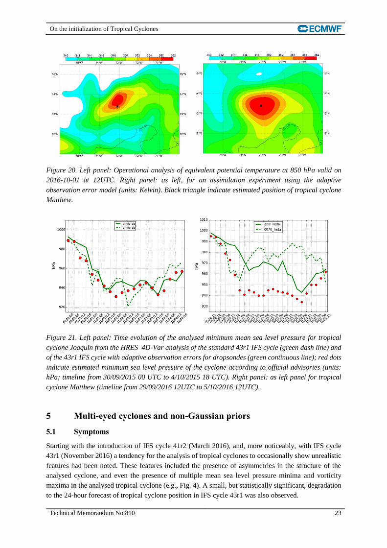
Figure 23. Evolution of the forecast globally averaged absolute pressure tendency for experiments from
IFS cycle 43r1 (black curve), IFS cycle 41r2 (red curve) and IFS cycle 41r1 (blue curve) during the first
12 hour of the forecast (unit: Pa/3hour).Curves are computed as average values over six assimilation
updates.

On the initialization of Tropical Cyclones
26 Technical Memorandum No.810
Figure 24. Evolution of the mean sea level pressure background forecast for the operational 43r1 IFS
cycle started on 2017-07-07 at 18UTC at t=0h (top left panel); t=3h (top right panel); t=6h (bottom left
panel); t=9h (bottom right panel). (Isolines increment: 1hPa).
Figure 25. Background forecast (right panel) and analysis of the mean sea level pressure field for the
operational 43r1 IFS cycle valid on 2017-07-08 at 00UTC in the vicinity of tropical cycle Eugene (black
diamond indicate estimated position of the cyclone at the analysis time). Wind arrows show observed
winds from ASCAT instrument valid on 2017-07-08 at 04.35UTC.
Figure 26. Background forecast (left panel) and EDA-estimated background errors (right panel) for the
mean sea level pressure field for the operational 41r2 IFS cycle valid on 2015-10-23 at 09UTC in the
vicinity of tropical cycle Patricia (black/red diamond indicate estimated position of the cyclone at the
nominal time); Units: hPa.

On the initialization of Tropical Cyclones
Technical Memorandum No.810 27
The appearance of multimodal error distributions in the tropical cyclone forecast position can be viewed
as a symptom of the increasing deviations from Gaussianity of the EDA forecast ensemble with
increasing resolution. This is apparent in Fig. 27 where the K2 D’Agostino diagnostic test of deviation
from normality (D’Agostino et al., 1990; Legrand et al., 2016) is presented for different resolutions of
the short range EDA background vorticity forecasts. The D’Agostino test highlights deviations from
normality due to how much the skewness and kurtosis of the sample distribution differ from those of a
Gaussian distribution: For normal distributions, the K2 diagnostic approximately follows a chi-squared
law with two degrees of freedom. The plots in Fig. 27 clearly show the increase in this measure of non-
Gaussianity as a function of the increase of the grid and, more sensitively, spectral resolution at which
the EDA ensemble forecast is sampled.
Figure 27. K2 D’Agostino test statistics of deviation from normality for EDA background forecasts of
vorticity at different resolutions: triangular spectral truncation 159 on linear reduced Gaussian grid
(TL159), triangular spectral truncation 159 on cubic octahedral reduced Gaussian grid (TCo159);
triangular spectral truncation 399 on linear reduced Gaussian grid (TL399).
5.2 Therapies
The diagnostics presented above indicate that increasing the small-scale contributions to the EDA-
derived background errors over recent IFS cycles has affected the analysis of tropical cyclones in two
ways: a) contributing to the increase in small-scale analysis increments and the noisiness of the ensuing
analyses and forecasts, and b) introducing non-Gaussian features in the diagnosed error distribution. As
a first step towards controlling these effects, it has been decided in IFS cycle 43r3 to reduce the
resolution of the EDA-derived background errors used in the 4D-Var analysis to spectral truncation
T159 on a linear reduced Gaussian grid. In combination with this change, the algorithm used to filter
small scale sampling noise from the EDA-derived errors has been changed from a spectral to a wavelet-
based approach (Bonavita et al., 2012). The wavelet approach has the advantage of allowing for spatial
variations in the filter, which can be useful if sampling errors show appreciable heterogeneity. This
appears to be case for the EDA-estimated errors, as confirmed in Figure 28. There we present the

On the initialization of Tropical Cyclones
28 Technical Memorandum No.810
diagnosed longitudinally averaged profile of the signal-to-noise ratio for the EDA-derived vorticity
background errors in the spectral range T127-159. It is apparent that the wavelet filter based on this
signal-to-noise diagnostic will be more active in suppressing small scale features in the tropical belt than
in the extra-tropics.
Figure 28. Longitudinal average of the signal-to-noise ratio for the EDA-derived vorticity background
errors in the spectral range T127-159. Model levels on y-axis.
The combination of reduced resolution of the background errors used in the analysis and the more
selective noise filter leads to a noticeable reduction of the magnitude of small scale increments above
spectral number 80 (Fig. 29, left panel); and to a small but consistent reduction of globally averaged
absolute pressure tendencies during the background forecast (Note however, how it still take approx. 9
hours for the adjustment process from the initial conditions to complete). As a result, initial conditions
and short range forecasts of tropical cyclones appear more axis-symmetric and less prone to develop
multiple centres (e.g., Fig. 30, to be compared with Fig. 24 for the case of tropical cyclone Eugene; and
Fig. 31, left panel, to be compared with Fig. 26, left panel, for the case of tropical cyclone Patricia). The
estimates of background errors also show less asymmetries and/or multi-modal features apparent in
previous IFS cycles (e.g., Fig. 31, right panel, to be compared with Fig. 26, right panel). More regular
background fields and unimodal background error structures finally result in more physically consistent
analyses of tropical cyclones (e.g., Fig. 32).

On the initialization of Tropical Cyclones
Technical Memorandum No.810 29
Figure 29. Left panel: Spectral decomposition of initial analysis increments for vorticity at model level
122 (approx. 925 hPa) in IFS cycle 43r1 (black curve) and in IFS cycle 43r3 (red curve). Units: s-1.
Right panel: Evolution of the forecast globally averaged absolute pressure tendency for experiments
from IFS cycle 43r1 (black curve), and IFS cycle 43r3 (red curve) during the first 12 hour of the forecast
(unit: Pa/3hour).Curves are computed as average values over six assimilation updates.
Figure 30. Evolution of the mean sea level pressure background forecast for the pre-operational 43r3
IFS cycle started on 2017-07-07 at 18UTC at t=0h (top left panel); t=3h (top right panel); t=6h (bottom
left panel); t=9h (bottom right panel). (Isolines increment: 1hPa).

On the initialization of Tropical Cyclones
30 Technical Memorandum No.810
Figure 31. Background forecast (left panel) and EDA-estimated background errors (right panel) for the
mean sea level pressure field for a 43r3 IFS cycle experiment valid on 2015-10-23 at 09UTC in the
vicinity of tropical cycle Patricia (black/red diamond indicate estimated position of the cyclone at the
nominal time); Units: hPa.
Figure 32. Cross section of tropical cyclone Patricia analysed relative vorticity field valid on 2015-10-
23 at 12UTC from reference 41r2 experiment (left) and a cycle 43r3 experiment with the changes
introduced to improve the initialization of tropical cyclones as described in the main text. Units: s-1.
6 Verification of Tropical Cyclones analyses and forecasts
The verification of tropical cyclones analyses and forecasts is mainly performed against official
estimates of the position and intensity as reported by one of the six tropical cyclone Regional Specialized
Meteorological Centres (RSMC) responsible for the basin in question. These estimates are in many cases
the only source of information available for verification. They are associated with position and intensity
uncertainties that are dependent on basin, cyclones intensity and to some extent the availability of other
in-situ observations. Position uncertainties are expected to be smaller for deep tropical cyclones (thanks
to their well-defined cloud patterns) but, in contrast, the intensity errors are believed to be significantly
larger. Occasionally the estimated minimum sea level pressure is kept at unrealistically constant levels

On the initialization of Tropical Cyclones
Technical Memorandum No.810 31
for many hours due the way detection techniques (e.g. Advanced Dvorak Technique, ADT: Olander and
Velden, 2007) work and the availability of microwave satellite observations (able to penetrate through
clouds). An example of this behaviour is given in Fig. 33 for TC Malakas. Best track data are a refined
estimates of the position and intensity but usually they are provided in a delayed mode (up to few months
later for some RSMCs). The other measurements of tropical cyclones intensity are also prone to errors
that are situation dependent. The main factors influencing observation errors are:
• Size and intensity of tropical cyclones
• Basin: different practices for each RSMC and typical environmental conditions (e.g. SST)
• Sampling issues (e.g. dropsondes)
• Limitations of TC tracking technics (e.g. ADT)
• Instrumentation errors
Figure 33. Verification of ECMWF HRES and ENS forecasts initialised on 2016-09-15 00UTC, for
tropical cyclone Malakas. Red circles represent the estimated minimum MSLP from the RSMC reports.
The verification of tropical cyclones analyses and forecasts is therefore complicated due to the varying
nature and magnitude of the errors in the RSMC advisories. In some situations, the magnitude of these
errors might even mask improvements made by the data assimilation. It is thus useful to be able to
verify the TC analyses and forecasts against a range of other available observations, e.g.: surface
pressure, 10m wind from scatterometer and wind/temperature from dropsondes. Differences between
the analysis and observations are routinely computed by the data assimilation system. Such comparison
can now be extended to medium range forecasts thanks to the computation of forecast departures
(Dahoui et al. 2016). The verification statistics can be computed for individual tropical cyclones or for
all tropical cyclones during a defined period. Statistics are generated using observations located within
a small moving area around tropical cyclones. Depending on the position of the tropical cyclone relative
to the progressing orbit of satellites, only part of the feature may be sampled by the scatterometer data,
both spatially and temporally. This type of verification is not meant to replace the standard verification
based on the official reports of track position and minimum pressure as provided by RSMCs, but to
complement it and extend to times when the standard verification is not available or it turns out to be
inaccurate (e.g., Fig. 34).
On the initialization of Tropical Cyclones
32 Technical Memorandum No.810
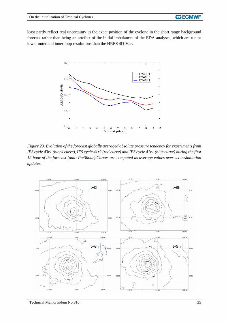
Figure 34. 10m wind from the ASCAT scatterometer on board METOP-A at 12.06 UTC on 2017-02-22
(green arrows) and their counterpart from the background forecast of the operational IFS near tropical
cyclone Alfred on 2017-02-22 at 12 UTC. Red triangle represents reported tropical cyclone location.
7 Discussion and research perspectives
The results and examples discussed in this paper show that providing an accurate and realistic
representation of the initial conditions of a tropical cyclone for NWP purposes can sometimes be
challenging. Sometimes the standard assumptions about the validity of the tangent linear hypothesis in
incremental 4D-Var fail. In addition, assumptions about normality and accuracy of the error models
used in the analysis update become increasingly less valid when using observations sampling the
atmosphere near the TC centre.
The problems seen in determining appropriate initial conditions for tropical cyclones have become more
frequent in the past few years, as the spatial resolution has increased in the IFS model, the analysis
system and the EDA-derived background errors. This is understandable because at the current resolution
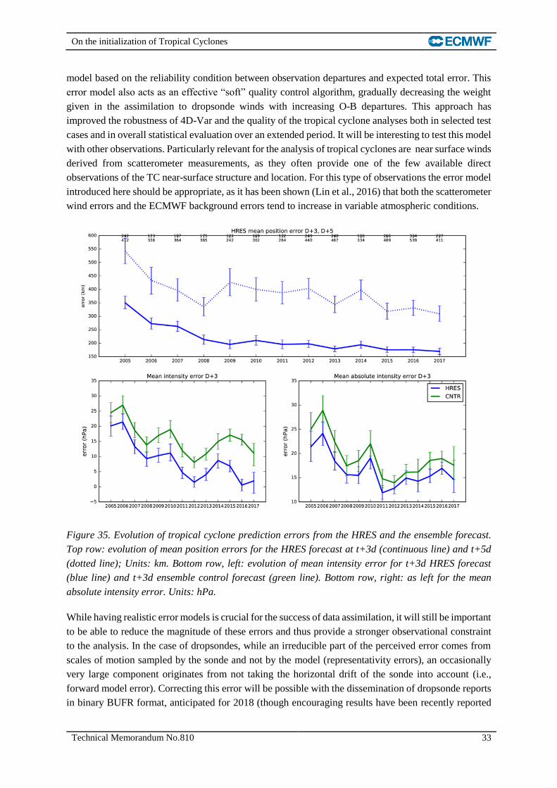
(TCo1279, approx. 9 km grid spacing) the IFS model is capable of forecasting tropical cyclones of
realistic intensity and structure (Fig. 35. Note how the mean intensity error of the t+3d forecast has
reduced close to zero in recent years). As the case of the dropsonde winds has highlighted, the
combination of realistic TC background forecasts with observations sampling the inner structure of a
tropical cyclone can produce observation departures an order of magnitude larger than the total
(background plus observation) expected error, or more. These conditions lead to the breakdown of the
tangent linear hypothesis in incremental 4D-Var and occasional numerical failures. Even when the
assimilation does not fail, results can be significantly degraded, as also reported in previous studies
(Harnisch and Weissman, 2010; Aberson, 2008). The solution proposed here is to account explicitly for
representativity and forward model errors of these observations through an adaptive observation error
On the initialization of Tropical Cyclones
Technical Memorandum No.810 33
model based on the reliability condition between observation departures and expected total error. This
error model also acts as an effective “soft” quality control algorithm, gradually decreasing the weight
given in the assimilation to dropsonde winds with increasing O-B departures. This approach has
improved the robustness of 4D-Var and the quality of the tropical cyclone analyses both in selected test
cases and in overall statistical evaluation over an extended period. It will be interesting to test this model
with other observations. Particularly relevant for the analysis of tropical cyclones are near surface winds
derived from scatterometer measurements, as they often provide one of the few available direct
observations of the TC near-surface structure and location. For this type of observations the error model
introduced here should be appropriate, as it has been shown (Lin et al., 2016) that both the scatterometer
wind errors and the ECMWF background errors tend to increase in variable atmospheric conditions.
Figure 35. Evolution of tropical cyclone prediction errors from the HRES and the ensemble forecast.
Top row: evolution of mean position errors for the HRES forecast at t+3d (continuous line) and t+5d
(dotted line); Units: km. Bottom row, left: evolution of mean intensity error for t+3d HRES forecast
(blue line) and t+3d ensemble control forecast (green line). Bottom row, right: as left for the mean
absolute intensity error. Units: hPa.
While having realistic error models is crucial for the success of data assimilation, it will still be important
to be able to reduce the magnitude of these errors and thus provide a stronger observational constraint
to the analysis. In the case of dropsondes, while an irreducible part of the perceived error comes from
scales of motion sampled by the sonde and not by the model (representativity errors), an occasionally
very large component originates from not taking the horizontal drift of the sonde into account (i.e.,
forward model error). Correcting this error will be possible with the dissemination of dropsonde reports
in binary BUFR format, anticipated for 2018 (though encouraging results have been recently reported

On the initialization of Tropical Cyclones
34 Technical Memorandum No.810
by reconstructing the position of the dropsonde from ancillary information present in current
alphanumerical reports, Aberson et al., 2017).
Another aspect studied in this report is the tendency of the IFS to occasionally produce analyses with
multiple TC cores in situations when imagery and/or other observational evidence points to the existence
of a single cyclone core. These effects have also become noticeable in conjunction with the increases in
recent IFS cycles of the horizontal resolution of the model, the data assimilation system and the
background errors used in 4D-Var. These resolution increases have in turn produced significant
increases in small-scale analysis increments in the lower model levels and a connected increase in the
level of gravity wave noise in the initial hours of the forecast. As a consequence of the adjustment
processes taking place in the first few hours of the forecast, the background can develop multiple TC
cores (visible as multiple MSLP minima and/or vorticity maxima) and this negatively affects the
following analysis. This behaviour is more apparent in cyclones in the early stage of their development
and/or poorly constrained by observations. Reducing the resolution of the background errors together
with the application of a heterogeneous noise filter (both implemented in IFS cycle 43r3, July 2017) has
proved effective in controlling the issues of multiple core TCs and, at the same time, improving the
convergence properties of the 4D-Var minimization. On the other hand, the short range background
forecasts still show evidence of initial imbalances and subsequent adjustment processes taking place in
the first 6-9 hours. It may thus be appropriate to look again at the current configuration of the variational
digital filter implemented in the IFS (Jc-DFI, Gauthier and Thépaut, 2001) and its effectiveness in
damping spurious oscillations in the model.
A more worrying pattern is the occasional occurrence of multiple error maxima in the EDA-derived
background errors near tropical cyclones. Due to the lower outer and inner resolutions employed in the
EDA 4D-Var, these multipole error structures do not usually originate from single EDA members
developing multiple minima but from increasing small scale variability in their predicted positions and
occasionally bad convergence of the analysis in individual members. This pattern can be seen as
symptomatic of a more general tendency of the EDA short range forecast ensemble to deviate from a
Gaussian distribution. Standard diagnostic tests of deviation from normality confirm that while this
effect is relatively small at spectral resolution T159, it is significant at spectral resolution T399. The
reduction in the resolution of the background errors used in 4D-Var thus appears to be not only a
practical step to control initial imbalances but also to be required to reduce non-Gaussian effects in the
EDA background forecast ensemble. Of course, if the accuracy of the short range forecast improves
enough as the resolution increases, that would also reduce the occurrence of multiple minima.
A more fundamental approach to reduce non-Gaussian effects in the EDA forecast ensemble and thus
improve the TC analyses entails an increased use of satellite observations to constrain the TC
environment and structure. Scatterometer wind observations provide near “all-weather” surface winds
with valuable information on the TC location and strength. Initial tests on increasing the density and
weight of scatterometer derived wind vectors in the IFS showed benefits in the resulting analyses of
selected tropical cyclones (De Chiara et al., 2017). Another potentially important source of observations
for the initialisation of tropical cyclones are satellite radiances in the “all-sky” framework (Bauer et al.,
2010; Geer et al., 2017). The ability to use satellite observations in cloudy and precipitating conditions
will be important in order to have an effective observational constrain on the TC vortex and its associated
rainbands. Further improvements are expected from developments towards extending the “all-sky”
approach to temperature-sounding microwave radiances and infrared radiances and from the use of
observations from future satellite-based cloud and precipitation radars (ECMWF/SAC/46(17)12). One

On the initialization of Tropical Cyclones
Technical Memorandum No.810 35
current limitation in the use of scatterometer winds and “all-sky” radiances is the need to use
considerably thinned datasets together with inflated error variances to deal with representativity errors
and significant spatial error correlations in the horizontal (De Chiara et al., 2017; Geer and Bauer, 2011).
It has however been shown (e.g., Rainwater et al., 2015) that correctly accounting for correlated errors
is important in recovering small-scale spatial information from observations. We thus expect that the
development of this capability in the IFS will prove beneficial to TC initialisation and to the analysis
accuracy in general.
Verification of the accuracy of tropical cyclone analyses and forecasts is typically done using best track
position and minimum pressure from RSMC advisories. This can be problematic for analyses and short-
range forecasts, when uncertainties in the reported position and the even larger uncertainties in the
estimated intensity of the TC are comparable to those of the NWP products. In these cases, we have
found useful to complement the standard verification with an observation-based approach, realised by
computing O-B and O-A statistics targeted to a moving area around the tropical cyclone.
8 Conclusions
Accurate forecasts of the trajectory and intensity of tropical cyclones are ever more important in order
to reduce their destructive impact on life and property. Increases in the resolution of atmospheric NWP
models and progress in the representation of physical processes have certainly helped improve the
ECMWF prognosis of TC evolution (e.g., Bechtold et al., 2012; Haiden et al., 2016), while promising
results have been obtained from a coupled Atmosphere-Ocean forecast configuration able to represent
aspects of the complex atmospheric and oceanographic interactions during tropical cyclone conditions
(Mogensen et al., 2017).
While improvements in the IFS model resolution and accuracy have been shown to be able to produce
increasingly realistic forecasts of tropical cyclones, they also present a more difficult problem to the
data assimilation system. This is because standard assumptions about representativity and forward
model errors, normality of background errors, validity of the tangent linear hypothesis and dynamical
balances in the analysis are called into question when the DA system has to deal with observations
sampling the tropical cyclone centre. In this sense, the initialisation of tropical cyclones can be seen as
a testbed for the performance of the DA system and its robustness in situations that can be very far from
climatological averages. From this perspective, the enhanced use of EDA information to characterise
observations errors in addition to background errors can be seen as a practical way to sample error
distributions under these conditions. More generally, increasing and improving the use of available
observations will be fundamental to our ability to provide accurate analyses and prognoses of tropical
cyclones and also to provide additional verification tools. Research activities in this direction are
ongoing and their results will be the subject of a future paper.
ACKNOWLEDGEMENTS
We gratefully acknowledge the contribution of Martin Janousek in providing the verification of
ECMWF tropical cyclones forecast skill shown in Fig. 35. We would also like to thank Sim Aberson
(Hurricane Research Division, NOAA) and Andrew Burton (Bureau of Meteorology, Australia) for their
helpful comments on earlier versions of this manuscript.

On the initialization of Tropical Cyclones
36 Technical Memorandum No.810
References
Aberson, S. D., 2008: Large forecast degradations due to synoptic surveillance during the 2004 and
2005 hurricane seasons. Mon. Wea. Rev., 136, 3138–3150, doi:10.1175/2007MWR2192.1.
Aberson, S.D., J. Cione, C.-C. Wu, M.M. Bell, J. Halverson, C. Fogarty, and M. Weissmann, 2010:
Aircraft observations of tropical cyclones. In Global Perspectives on Tropical Cyclones: From Science
to Mitigation, J.C.L. Chan and J.D. Kepert (Eds.). World Scientific Publishing Company, 2nd edition,
pp 227-240
Aberson, S.D., K.J. Sellwood, and P.A. Leighton, 2017: Calculating Dropwindsonde Location and Time
from TEMP-DROP Messages for Accurate Assimilation and Analysis. J. Atmos. Oceanic Technol., 34,
1673–1678, https://doi.org/10.1175/JTECH-D-17-0023.1
Bauer, P., Geer, A. J., Lopez, P. and D. Salmond, 2010: Direct 4D-Var assimilation of all-sky radiances.
Part I: Implementation. Q.J.R. Meteorol. Soc., 136: 1868–1885. doi:10.1002/qj.659
Bechtold, P., P. Bauer, P. Berrisford, J.R. Bidlot, C. Cardinali, T. Haiden, M. Janousek, D. Klocke, L.
Magnusson, A. McNally, F. Prates, M. Rodwell, N. Semane and F. Vitart, 2012: Progress in predicting
tropical systems: The role of convection. Technical Memorandum 686, ECMWF. Available at
https://www.ecmwf.int/en/elibrary/technical-memoranda
Bonavita M, Isaksen L, Hólm E.V., 2012: On the use of EDA background-error variances in the
ECMWF 4D-Var. Q. J. R. Meteorol. Soc. 138: 1540–1559, doi:10.1002/qj.1899.
Chen, Y., and C. Snyder, 2007: Assimilating vortex position with an ensemble Kalman Filter. Monthly
Weather Review, 135, 1828-1845.
Courtier, P., Thepaut, J.-N. and A. Hollingsworth, 1994: A strategy for operational implementation of
4D-Var, using an incremental approach. Q. J. R. Meteorol. Soc., 120, 1367-1387.
D’Agostino, R.B., A. Belanger and D’Agostino, R.B.Jr, 1990: A suggestion for using powerful and
informative tests of normality, The American Statistician, 44(4): 316-321.
Dahoui, M., G. Radnoti, S. Healy, L. Isaksen, and T. Haiden, 2016: Use of forecast departures in
verification against observations. ECMWF Newsletter No. 149, 30-33. Available at
https://www.ecmwf.int/sites/default/files/elibrary/2016/16759-newsletter-no149-autumn-2016.pdf
Daley, R., 1993: Estimating observation error statistics for atmospheric data assimilation. Ann.
Geophysicae, 11, 634-647.
De Chiara, G., M. Bonavita and S. J. English, 2017: Improving the assimilation of scatterometer wind
observations in global NWP, IEEE J. Sel. Topics Appl. Earth Obs. Remote Sens.,
doi:10.1109/JSTARS.2017.2691011
Doocy S., A. Dick, A. Daniels and T.D. Kirsch, 2013: The Human Impact of Tropical Cyclones: a
Historical Review of Events 1980-2009 and Systematic Literature Review. PLOS Currents Disasters.
2013 Apr 16. Edition 1. doi: 10.1371/currents.dis.2664354a5571512063ed29d25ffbce74.

On the initialization of Tropical Cyclones
Technical Memorandum No.810 37
ECMWF SAC Paper: ECMWF/SAC/46(17)12: Assimilating observations sensitive to cloud and
precipitation, 2017. Available at https://www.ecmwf.int/en/about/who-we-are/governance/sac/46-0.
Gauthier, P. and J. Thépaut, 2001: Impact of the Digital Filter as a Weak Constraint in the Preoperational
4DVAR Assimilation System of Météo-France. Mon. Wea. Rev., 129, 2089–2102,
https://doi.org/10.1175/1520-0493(2001)129<2089:IOTDFA>2.0.CO;2
Geer, A. J. and P. Bauer, 2011: Observation errors in all-sky data assimilation. Q.J.R. Meteorol. Soc.,
137: 2024–2037. doi:10.1002/qj.830
Geer, A. J., F. Baordo, N. Bormann, S. English, M. Kazumori, H. Lawrence, P. Lean, K. Lonitz, and C.
Lupu, 2017: The growing impact of satellite observations sensitive to humidity, cloud and precipitation.
Quart. J. Roy.Meteorol. Soc., in review.
Haiden, T., Janousek, M., Bidlot, J., Ferranti, L., Prates, F., Vitart, F., Bauer, P., Richardson, D.S., 2016:
Evaluation of ECMWF forecasts, including the 2016 resolution upgrade. Technical Memorandum 792,
ECMWF. Available at https://www.ecmwf.int/en/elibrary/technical-memoranda.
Harnisch, F. and M. Weissmann, 2010: Sensitivity of Typhoon Forecasts to Different Subsets of
Targeted Dropsonde Observations. Mon. Wea. Rev., 138, 2664–2680,
https://doi.org/10.1175/2010MWR3309.1
Heming, J. T. 2016: Met Office Unified Model Tropical Cyclone Performance Following Major
Changes to the Initialization Scheme and a Model Upgrade. Wea. Forecasting, 31, 1433–1449,
https://doi.org/10.1175/WAF-D-16-0040.1
Holm, E. V., M. Bonavita and L. Magnusson, 2015: Improved spread and accuracy in higher-resolution
ensemble of Data Assimilations. ECMWF Newsletter No. 145. Available at
https://www.ecmwf.int/sites/default/files/elibrary/2015/14589-newsletter-no145-autumn-2015.pdf
Hopson, T.M., 2012: Assessing the Ensemble Spread-Error Relationship. Monthly Weather Review,
142, 1125-1142.
Houtekamer, P.L. 1993: Global and Local Skill Forecasts. Monthly Weather Review, 121, 1834-1846.
Huber, P.J., 1964: Robust estimates of a location parameter. Ann. Math. Stat. 35: 73–101.
Ingleby, 2017: An assessment of different radiosonde types 2015/2016. ECMWF Technical
Memorandum 807, ECMWF. Available at https://www.ecmwf.int/en/elibrary/technical-memoranda.
Ingleby, B. and D. Edwards, 2015: Changes to radiosonde reports and their processing for numerical
weather prediction, Atmosph. Sci. Lett., 16: 4449. doi:10.1002/asl2.518.
Ingleby B., P. Pauley, A. Kats, J. Ator, D. Keyser, A. Doerenbecher, E. Fucile, J. Hasegawa, E. Toyoda,
T. Kleinert, W. Qu, J. St James, W. Tennant, R. Weedon, 2016: Progress towards high-resolution, real-
time radiosonde reports. Bull. Amer. Meteor. Soc., 97, 2149–2161, doi: 10.1175/BAMS-D-15-
00169.1.

On the initialization of Tropical Cyclones
38 Technical Memorandum No.810
Isaksen, L., M. Bonavita, R. Buizza, M. Fisher, J. Haseler, M. Leutbecher and L. Raynaud, 2010:
Ensemble of data assimilations at ECMWF. Technical Memorandum 636, ECMWF. Available at
https://www.ecmwf.int/en/elibrary/technical-memoranda.
Janisková, M., and P. Lopez, 2013: Linearized physics for data assimilation at ECMWF. In: S.K. Park
and L. Xu (eds.), Data assimilation for Atmospheric, Oceanic and Hydrological Applications(Vol. II),
doi: 10.1007/978-3-642-35088-7, ©Springer-Verlag Berlin Heidelberg, 251-286.
Janjic, T. and S.E. Cohn, 2006: Treatment of observation errors due to unresolved scales in atmospheric
data assimilation. Monthly Weather Review, 134, 2900-2915.
Kleist, D. T., 2011: Assimilation of tropical cyclone advisory minimum sea level pressure in the NCEP
Global Data Assimilation System. Wea. Forecasting, 26, 1085–1091, doi:10.1175/WAF-D-11-00045.1.
Legrand, R., Y. Michel and T. Montmerle 2016: Diagnosing non-Gaussianity of forecast and analysis
errors in a convective-scale model. Nonlin. Processes Geophys., 23, 1-12, https://doi.org/10.5194/npg-
23-1-2016.
Lin, W., Portabella, M., Stoffelen, A., Vogelzang, J. and A. Verhoef, A., 2016: On mesoscale analysis
and ASCAT ambiguity removal. Q.J.R. Meteorol. Soc., 142: 1745–1756. doi:10.1002/qj.2770
Liu, Z.-Q., and F. Rabier, 2002: The interaction between model resolution, observation resolution and
observation density in data assimilation: A one dimensional study. Q. J. R. Meteorol. Soc., 128, 1367-
1386.
Lorenc, A.C., 1986: Analysis methods for numerical weather prediction. Q. J. R. Meteorol. Soc., 112,
1177-1194.
Mogensen, K.S., L. Magnusson, J.R. Bidlot, 2017: Tropical Cyclone Sensitivity to Ocean Coupling.
Technical Memorandum 794, ECMWF. Available at https://www.ecmwf.int/en/elibrary/technical-
memoranda.
Olander, T.L. and C.S. Velden, 2007: The Advanced Dvorak Technique: Continued Development of an
Objective Scheme to Estimate Tropical Cyclone Intensity Using Geostationary Infrared Satellite
Imagery. Wea. Forecasting, 22, 287–298, https://doi.org/10.1175/WAF975.1
Rainwater, S., Bishop, C. H. and W. F. Campbell, 2015: The benefits of correlated observation errors
for small scales. Q.J.R. Meteorol. Soc., 141: 3439–3445. doi:10.1002/qj.2582
Stewart, S.R., 2017: Hurricane Matthew Tropical Cyclone Report (AL142016). National Hurricane
Center, NOAA. Available at http://www.nhc.noaa.gov/data/tcr/AL142016_Matthew.pdf
Tavolato, C. and Isaksen, L., 2015: On the use of a Huber norm for observation quality control in the
ECMWF 4D-Var. Q.J.R. Meteorol. Soc., 141: 1514–1527. doi:10.1002/qj.2440
Torn, R. D., and G. J. Hakim, 2009: Ensemble data assimilation applied to RAINEX: Observations of
Hurricane Katrina, 2005: Monthly Weather Review, 137, 2817-2829.

On the initialization of Tropical Cyclones
Technical Memorandum No.810 39
Torn, R. D., 2010: Performance of a mesoscale ensemble Kalman Filter (EnKF) during the NOAA
high-resolution hurricane test. Monthly Weather Review, 138, 4375{4392.
Trahan, S., and L. Sparling, 2012: An analysis of NCEP tropical cyclone vitals and potential effects on
forecasting models. Wea. Forecasting, 27, 744-756. Doi:10.1175/WAF-D-11-00063.1
Waller, J. A., Dance, S. L., Lawless, A. S., Nichols, N. K. and Eyre, J. R., 2014: Representativity error
for temperature and humidity using the Met Office high-resolution model. Q.J.R. Meteorol. Soc., 140:
1189–1197. doi:10.1002/qj.2207
Weissmann, M., F. Harnisch, C. Wu, P. Lin, Y. Ohta, K. Yamashita, Y. Kim, E. Jeon, T. Nakazawa,
and S. Aberson, 2011: The Influence of Assimilating Dropsonde Data on Typhoon Track and
Midlatitude Forecasts. Mon. Wea. Rev., 139, 908-920, https://doi.org/10.1175/2010MWR3377.1
Whitaker, J.S. and A.F. Loughe, 1998: The Relationship between Ensemble Spread and Ensemble Mean
Skill. Monthly Weather Review, 126, 3292-3302.
Yamaguchi, M., M. Nakagawa, J. Ishida and H. Sato, 2017: WGNE Intercomparison of
Tropical Cyclone Forecasts by Operational NWP Models: A Quarter-Century and Beyond. Bull. Amer.
Meteor. Soc. doi:10.1175/BAMS-D-16-0133.1, in press.