NUHEP-TH/19-012, FERMILAB-PUB-19-508-T

On the Impact of Neutrino Decays on the Supernova Neutronization-Burst Flux

Andre de Gouvea,1, ∗ Ivan Martinez-Soler,1, 2, 3, † and Manibrata Sen1, 4, ‡

1Northwestern University, Department of Physics & Astronomy, 2145 Sheridan Road, Evanston, IL 60208, USA2Theory Department, Fermi National Accelerator Laboratory, P.O. Box 500, Batavia, IL 60510, USA

3Colegio de Fısica Fundamental e Interdisciplinaria de las Americas (COFI),254 Norzagaray street, San Juan, Puerto Rico 00901.

4Department of Physics, University of California Berkeley, Berkeley, California 94720, USA

The discovery of non-zero neutrino masses invites one to consider decays of heavier neutrinos intolighter ones. We investigate the impact of two-body decays of neutrinos on the neutronization burstof a core-collapse supernova – the large burst of νe during the first 25 ms post core bounce. In themodels we consider, the νe, produced mainly as a ν3 (ν2) in the normal (inverted) mass ordering,are allowed to decay to ν1 (ν3) or ν1 (ν3) , and an almost massless scalar. These decays can leadto the appearance of a neutronization peak for a normal mass ordering or the disappearance of thesame peak for the inverted one, thereby allowing one mass ordering to mimic the other. Simulatingsupernova-neutrino data at the Deep Underground Neutrino Experiment (DUNE) and the Hyper-Kamiokande (HK) experiment, we compute their sensitivity to the neutrino lifetime. We find that, ifthe mass ordering is known, and depending on the nature of the Physics responsible for the neutrinodecay, DUNE is sensitive to lifetimes τ/m . 106 s/eV for a galactic SN sufficiently close-by (around10 kpc), while HK is sensitive to lifetimes τ/m . 107 s/eV. These sensitivities are far superior toexisting limits from solar-system-bound oscillation experiments. Finally, we demonstrate that usinga combination of data from DUNE and HK, one can, in general, distinguish between decaying Diracneutrinos and decaying Majorana neutrinos.

I. INTRODUCTION

The fact that neutrinos have nonzero masses [1] invites several questions related to other unknown neutrino proper-ties, among those the values of the neutrino lifetimes. Given everything currently known about the neutrinos, one canaffirm that the two heavier neutrinos – ν3 , ν2 in the case of the so-called normal mass ordering (NMO), ν2 , ν1 in thecase of the so-called inverted mass ordering (IMO) – have nonzero mass and finite lifetime [2–8]. Assuming no newinteractions or degrees of freedom, the heavier neutrinos decay, at the one-loop level, to either another neutrino anda photon, νh → νlγ, or to three lighter neutrinos, νh → νlνlνl, where h refers to a heavier neutrino mass-eigenstate,l to a lighter one. Under the same assumptions, because neutrino masses are tiny, the expected lifetimes are manyorders of magnitude longer than the age of the universe.

New interactions and degrees of freedom will, of course, lead to potentially much shorter lifetimes. One possibility,which we consider in this paper, is the introduction of a new (almost) massless scalar, which can couple to theneutrinos [3, 9–13]. This allows for the decay of the heavy neutrino into a lighter neutrino and the scalar. In thesescenarios, the daughter neutrinos can play a significant role, as we describe in Section II. The nature of the neutrinos– Dirac versus Majorana – and the helicity-structure of the interaction [7, 14–17] also play an important role sincethey render the daughter visible or invisible, or render the (effective) lepton-number the same as or different fromthat of the parent.

Different experimental constraints have been placed on the lifetime of the neutrinos, ranging from bounds fromterrestrial neutrinos to the study of neutrinos produced in astrophysical sources [14, 15, 17–40]. Roughly speaking,the idea is simple: if neutrinos are produced in a relatively well-characterized source and measured a certain knowndistance away from the source, the fact that they make it to the detector implies, in a very model-independent way,that the neutrinos are not disappearing along the way. All bounds are much smaller than the expectations of thestandard-three-neutrinos-paradigm and the age of the universe.

The best, mostly model-independent bounds on the decays of ν2 and ν1 come from the analysis of solar neutrinos

∗Electronic address: degouvea@northwestern.edu†Electronic address: ivan.martinezsoler@northwestern.edu‡Electronic address: manibrata@berkeley.edu

arX

iv:1

910.

0112

7v2

[he

p-ph

] 2

4 Ja

n 20

20

2

[22, 27]. Using mostly the 8B solar neutrino data, one is sensitive to τ2/m2 < 10−3 s/eV∗ [27], while, using mostly the7Be and low energy pp neutrino data [41], one is sensitive to τ1/m1 < 10−4 s/eV [27]. Considering invisible decays,the current bounds imposed from the analysis of the SNO data, combined with other solar neutrino experiments,results in the lifetime of τ2/m2 > 1.92 × 10−3 s/eV at 90% confidence [42]. Since |Ue3|2 is very small, solar data arevery inefficient when it comes to constraining the lifetime of ν3. Constraints on the ν3 lifetime can be obtained fromatmospheric and beam neutrino experiments. Recent bounds on the ν3 lifetime were estimated using atmosphericdata: τ3/m3 > 10−10 s/eV [31, 36]. Clearly, these bounds are much weaker than the ones on the ν1 and ν2 lifetimes.Slightly more stringent bounds [15, 37] are expected from next-generation neutrino oscillation experiments includingthe JUNO [43] and DUNE [44] experiments, while stronger but model-dependent bounds – τ3/m3 > 2.2× 10−5 s/eV– from solar neutrinos have been recently proposed [17].

These rather loose bounds lead one to explore baselines which are much longer than one Astronomical Unit. Twocandidates immediately qualify for the search: (i) neutrinos from supernova SN1987A [45–50], and (ii) ultra-high-energy neutrinos from astrophysical sources, detected at IceCube [51, 52]. Constraints from SN1987A were pursuedin the literature [29, 53], while constraints from IceCube – current and future – are plagued by uncertainties on theneutrino flavor composition [54, 55]. Here we concentrate on the next galactic supernova as a probe of long lifetimesfor the neutrinos.

A core-collapse supernova (SN) emits almost 99% of its binding energy in the form of neutrinos (see [56] for a detailedreview). During, roughly, the first 25 ms post core-bounce, a large burst of electron neutrinos is emitted due to thedeleptonization of the core. This phase, known as the “neutronization burst”, is a robust prediction of all core-collapseSN simulations. During the neutronization burst, negligible amounts – relative to that of νe – of νe and νµ, τ , νµ, τare released. This implies that the neutronization-burst flux does not undergo significant collective oscillations but ismostly processed by the well-understood Mikheyev-Smirnov-Wolfenstein (MSW) resonant flavor conversion [57, 58]associated to the ordinary matter density the neutrinos encounter on their way our of the supernova. This implies thatthe flavor-evolution of these neutrinos is not impacted by large uncertainties associated with collective oscillations[59–71]. This renders the neutronization-burst neutrinos well suited for performing robust tests of neutrino properties.We provide a detailed description of these neutrinos in Section III.

A detailed analysis allowing for the decay of the heavier neutrinos during the neutronization burst was first per-formed in [25]. It was argued that the νe, propagating as a heavy mass-eigenstate νh, could decay into a lighterνl during its flight. Considering a simple Majoron-like model, with scalar as well as pseudo-scalar couplings, theauthor studied the presence of a sharp neutronization peak due to νe in water-Cherenkov detectors. Here, we exploredifferent scenarios that lead to neutrinos decaying into a scalar and a lighter neutrino, and concentrate on severalphysics questions. First, we discuss whether the hypothesis that neutrinos have a finite lifetime can hinder the abilityof measurements of the next galactic supernova neutrinos to determine the neutrino mass-ordering. Second, assum-ing the mass ordering is known, we characterize how well measurements of the neutrinos from a galactic supernovaexplosion can be used to measure or place bounds on the neutrino lifetimes. Finally, we discuss how different measure-ments of the neutronization-burst neutrinos can be used to distinguish different neutrino-decay scenarios and provideinformation on the nature of the neutrino.

Our strategy is as follows. Using the results of the hydrodynamical simulations of the Garching group for a 25M�progenitor model [72], we study the neutronization-burst flux in the presence of a neutrino two-body decay, νi →

(−)

νj ϕ,where ϕ is a massless scalar; the details are spelled out in Section IV. We analyze the signatures of this decay inthe upcoming DUNE experiment [44], and the Hyper-Kamiokande (HK) experiment [73]. We find that for a typicalsupernova located at a distance of 10 kpc, these experiments are sensitive to lifetimes τ/m . 105−107 s/eV, which aremuch longer than what is currently constrained by solar and long-baseline neutrino data. Furthermore, since DUNEis mainly sensitive to the νe spectrum, while HK is mostly sensitive to the νe spectrum, a combination of these twoexperiments may be able to inform the Majorana versus Dirac question. Details of our simulation are described inSection V while our results are discussed in Section VI. We offer some concluding remarks in Section VII.

∗ All neutrinos ever observed are ultra-relativistic in the lab frame and hence one is only sensitive to the ratio τ/m. The fact that theneutrino masses are not known with any precision leads one to always quote the constraints on the neutrino lifetime as constraints inτ/m. Historically, the literature prefers to quote bounds on τ/m in units of second per electronVolt. In “oscillation-equivalent units,”[27] 1 eV/s = 6.58× 10−16 eV2.

3

II. NEUTRINO DECAY INTO A SCALAR AND A LIGHTER NEUTRINO

In this section, we discuss different scenarios that allow for the two-body decay of the neutrino mass-eigenstates,where the heaviest neutrino (νh) decays to a lighter neutrino (νl), and a scalar field with negligible mass. We considerthe possibility that the neutrinos are massive Majorana or Dirac fermions. For concreteness, we will concentrateon the NMO and the scenario where the heaviest neutrino (h = 3) decays to the lightest neutrino (l = 1), unlessotherwise noted. We will also ignore the mass of the scalars and the lighter neutrino. It should be clear that all theresults to be derived here apply to, for example, the IMO and the scenario where the heaviest neutrino (h = 2) decaysto the lightest neutrino (l = 3). In the next sections, we will also make reference to this decay.

A. Dirac neutrinos

We augment the standard model Lagrangian by postulating the existence of new scalar fields. For simplicity andin order to avoid further problems, we assume the new scalar fields are singlets of the standard model gauge groupand only concentrate on the lowest-dimensional couplings of these to the standard model neutrinos. If the neutrinosare Dirac fermions, lepton number is a conserved global symmetry and we can classify the new scalars according tohow they transform under U(1)L – lepton-number symmetry. We will consider two simple cases: lepton-number zeroscalars and lepton-number two scalars.

A scalar field ϕ0 with zero lepton number can couple to neutrinos only at the dimension-five level:

LDir ⊃gijΛ

(LiH)νcjϕo + h.c. ⊃ gijνiνcjϕ0 + h.c. , (II.1)

where gij = gijv/Λ, Λ is the effective scale of the operator and v is the vacuum expectation value of the neutralcomponent of the Higgs field. Here and throughout we express all fermions as left-handed Weyl fields; νci are theleft-handed antineutrino fields while Li are the standard model lepton doublets. The indices i, j = 1, 2, 3 run over thedifferent neutrino mass eigenstates.

In the laboratory frame, the decay width of such a process is

Γ =g2m2

3

64πE3, (II.2)

where g2 = |g13|2 + |g31|2, m3 is the mass of ν3, and E3 its energy. This decay-width is related to the lifetime, τ3 inthe ν3 rest-frame: τ3 = m3/(E3 Γ).

We will be interested in ν3’s produced via the weak interactions under conditions where, in the laboratory frame,E3 � m3 so the ν3 beam will be, effectively, left-handed. After the ν3 decay, the daughter ν1 may be either left-handedor right-handed. The energy distributions of the daughter neutrinos in the laboratory frame are

ψh.c.(E3, E1) ≡ 1

Γ

dΓ

dE1∝ 2E1

E23

for ν3L → ν1L + ϕ0 ,

ψh.f.(E3, E1) ≡ 1

Γ

dΓ

dE1∝ 2

E3

(1− E1

E3

)for ν3L → ν1R + ϕ0 , (II.3)

for the helicity-conserving (h.c.) and helicity-flipping (h.f.) cases respectively. Here ‘L’ and ‘R’ stand for left andright helicity of the neutrinos. In the helicity-conserving case, the ν1 spectrum is harder. This is easy to understandfrom simple angular momentum conservation considerations. In the ν3 rest frame, the daughter neutrinos that sharethe same polarization as the parent are emitted preferentially in the direction of the polarization of the parent, whilethose with the opposite polarization are preferentially emitted in the opposite direction. In the reference frame wherethe parent is boosted, the daughters with the same helicity as the parent are emitted predominantly in the forwarddirection (higher energy), while the opposite-helicity daughters are emitted preferentially backwards (lower energy).

Ignoring effects proportional to the mass of the daughter neutrino (m1), the helicity-flipping channel producesneutrinos of the “wrong” helicity, i.e, right-handed neutrinos, which are effectively (and very safely) invisible toany detector. The relative weights of the helicity-flipping and helicity-conserving channels depend on the relativemagnitudes of g13 and g31, related to how much the new interactions violate parity. In maximally parity violatingscenarios, the ν3 decay may be completely invisible or completely visible. For concreteness, when we discuss thisϕ0-model quantitatively, we will always impose the constraint gij = gji, in such a way that the physics that describesneutrino decay is parity conserving. In this case, half of the neutrino daughters from the decay of a heavier neutrino

4

will be of the “correct” helicity while the other half will be of the “wrong” helicity.A scalar field ϕ2 with lepton-number two can couple to neutrinos only at dimension-four and dimension-six [74]:

LDir ⊃yij2νci ν

cjϕ2 +

hij2Λ2

(LiH)(LjH)ϕ∗2 + h.c , (II.4)

where, after spontaneous symmetry breaking, the second term includes hijνiνjϕ, hij = hijv2/Λ2. Here, Λ is the

effective scale of the dimension-six operator and yij = yij and hij = hji.Since ϕ2 carries lepton-number, Eq. (II.4) mediates the following decay: ν3 → ν1ϕ2; the neutrino lepton-number

changes by two units. Assuming yij � hij , (or vice-versa), the interactions in Eq. (II.4) are strongly parity violatingand the decays yield strongly polarized daughters. If yij � hij , all daughters will be of the “wrong-helicity” typeand hence invisible assuming an ultra-relativistic parent beam produced via the weak interactions (i.e., in the decayν3L → ν1ϕ2 all ν1 will be left-handed and hence invisible in the limit m1/E1 → 0). Instead, If hij � yij , all thedaughters will be of the “correct-helicity” and hence expected to interact in a neutrino detector (i.e., in the decayν3L → ν1ϕ2 all ν1 will be right-handed and hence visible in the limit m1 → 0). In both cases, the energy distributionsare as prescribed in Eqs. (II.3), where the invisible decays (yij � hij) follow the helicity-conserving equation, whilethe visible decays hij � yij follow the helicity-flipping one.

B. Majorana neutrinos

If the neutrinos are Majorana fermions, lepton number is explicitly broken and there is no need for light right-handed-neutrino degrees of freedom. If a new gauge-singlet scalar ϕ is added to the standard model particle content,the most minimal interaction that leads to the neutrino decays of interest is dimension-six:

LMaj ⊃fij2Λ2

(LiH)(LjH)ϕ+ h.c. ⊃ fij2

(νL)i(νL)jϕ+ h.c. , (II.5)

where fij = fji, fij = fijv2/Λ2 and Λ is the effective scale of the dimension-six operator. Here it is not meaningful

to assign lepton-number to ϕ.Here, in the laboratory frame, the decay width for ν3 → ν1 + ϕ is

Γ = 2× f2m23

64πE3, (II.6)

where f ≡ f13, m3 is the mass of ν3, and E3 its energy. This decay-width is related to the lifetime τ3 in the ν3

rest-frame: τ3 = m3/(E3 Γ). For Majorana neutrinos, the decay rates are twice as large as that of Dirac neutrinos(Eq. (II.2)) since one is compelled to include both the “neutrino” and “antineutrino” final states.

In the limit m1/E1 → 0, it is convenient to identify the two different helicity states of ν1 as the “neutrino”(ν1L) and the “antineutrino” (ν1R) where the charged-current scattering of the ν1 state leads to the production ofnegatively charged leptons while that of ν1 leads to positively charged leptons. In this case, Eq. (II.5) mediates bothν3L → ν1L + ϕ, and ν3L → ν1R + ϕ, both of which are visible modes. Furthermore, as long as the ν1 mass is smallenough, the energy distributions are also given by Eq. (II.3) [7, 14]; the “neutrino” final state is helicity-conserving,while the “antineutrino” final state is helicity-flipping. The relative-branching ratios, on the other hand, are the same.

C. Majorana versus Dirac

In general, Majorana and Dirac neutrino decays are distinguishable as long as one can measure the daughterneutrinos. In the ϕ0-model (Eq. (II.1)), heavier neutrinos decay to lighter visible neutrinos (or invisible neutrinos)while in the ϕ2-model (Eq. (II.4)), heavier neutrinos decay exclusively into visible antineutrinos (hij � yij) or invisibleantineutrinos yij � hij). The two models are distinguishable, in principle, if a nonzero fraction of the decays is visible.

Instead, in the Majorana case, heavier neutrinos decay into both visible lighter “neutrinos” and “antineutrinos”,and the branching ratios are the same. This means that if heavy neutrinos are produced in some far away sourcevia weak-interaction processes involving, say, negatively charged leptons (for example the deleptonization process ofinterest here, e− + p → n + ν) and only one new light scalar exists, Dirac neutrinos will decay into either neutrinosor antineutrinos. Majorana neutrinos, on the other hand, will decay into both “neutrinos” and “antineutrinos.”

5

The result above can be clouded by postulating more light degrees of freedom. If, for example, one combines theϕ0-model with the ϕ2-model, it is possible to choose couplings in such a way that a Dirac ν3 decays both into ν1 +ϕ0

and ν1 + ϕ2 with the same branching ratio. If this were the case, the Dirac neutrino case would perfectly mimic theMajorana one. On the other hand, if a new light fermionic degree of freedom exists, it is possible to write down aninteraction like Eq. (II.1) for Majorana neutrinos, where the left-handed antineutrino field is replaced by the new,sterile fermion. In this case, it is possible to have the Majorana neutrino case perfectly mimic the Dirac one. Weconsider both of these scenarios rather finely tuned and will ignore them henceforth.

Note that Eqs. (II.3) are, strictly speaking, only true if there exists a large hierarchy between the masses of theneutrinos, i.e., m3 � m1 [14]. If the neutrino masses are quasi-degenerate such that m3 ∼ m1 (keeping ∆m2

31 withinobservational bounds), then the helicity-flipping channel is suppressed. However, this does not impact our results forthe ϕ0-model, as the helicity-flipping channel is not detected. On the other hand, the helicity-flipping channel playsan important role for the ϕ2 model, or if the neutrinos are Majorana. As a result, the conclusions inferred in thesecases will have to be revised for the quasi-degenerate scenario. We will consider the neutrino masses to be hierarchical,and not focus on the quasi-degenerate limit in the rest of the paper.

D. Order of Magnitude Considerations

Before discussing the supernova explosion as a source of neutrinos and how the propagation of supernova neutrinosis impacted by – and informs – the neutrino lifetime, it is useful to estimate the naive sensitivity of supernova neutrinosto the neutrino lifetime. Lifetime effects are visible when Γ × L & 1, where L is the neutrino propagation distance.In the case of the ϕ0-model with Dirac neutrinos, this translates into

|g| & 2.3× 10−9

(E3

10 MeV

)1/2(10 kpc

L

)1/2 (0.5 eV

m3

). (II.7)

Similar values for the relevant couplings are obtained for the other models discussed in this section. This implies thesystems under investigation here are sensitive to very weakly-coupled new degrees of freedom. This, in turn, impliesthat virtually all laboratory probes – and many early universe probes – will not be as sensitive to this type of newphysics as the observables we are discussing here. There are a few exceptions; we comment on these in the concludingsection.

The constraint Γ× L & 1 can be re-expressed as τ/m . L/E† or

τ

m. 105 s/eV

(L

10 kpc

)(10 MeV

E

). (II.8)

This implies that supernova neutrinos produced 10 kpc away are sensitive to neutrino lifetimes that approach a fewdays for neutrino masses of order 1 eV.

III. FLAVOR EVOLUTION DURING THE NEUTRONIZATION BURST

Modern day simulations of core-collapse supernovae including a detailed treatment of the neutrino transport problemagree on the presence of the neutronization-burst phase that occurs typically for around 25 ms, immediately aftercore-bounce [75]. The core-collapse shock, launched as a result of the stiffening of the core, results in the dissociation ofthe surrounding nuclei into individual neutrons and protons. The newly formed protons capture electrons, producinga large burst of νe, thereby leading to the prompt deleptonization of the core. As the shock reaches relatively lowerdensities, these νe can stream out, leading to the neutronization burst. During this period, the other types of neutrinos– νe, as well as the other flavors (νµ, νµ, ντ , ντ ) – are also emitted, but the associated fluxes are very small whencompared to that of the νe.

A SN acts like an approximate blackbody, and cools by the emission of neutrinos. Keeping this in mind, SN

† L(m/E) is the baseline in the neutrino rest-frame.

6

νe

νe

νx

0 20 40 60 80 100

0

100

200

300

t (ms)

Lν(⨯

10

51

erg

s-

1)

νe

νe

νx

0 20 40 60 80 100

0

5

10

15

t (ms)

⟨Eν⟩

νe

νe

νx

0 20 40 60 80 1000

5

10

15

t (ms)

α

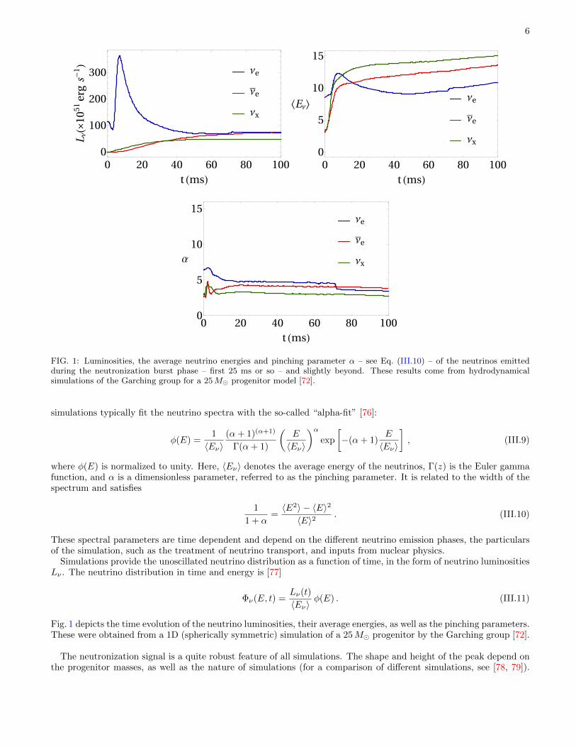
FIG. 1: Luminosities, the average neutrino energies and pinching parameter α – see Eq. (III.10) – of the neutrinos emittedduring the neutronization burst phase – first 25 ms or so – and slightly beyond. These results come from hydrodynamicalsimulations of the Garching group for a 25M� progenitor model [72].

simulations typically fit the neutrino spectra with the so-called “alpha-fit” [76]:

φ(E) =1

〈Eν〉(α+ 1)(α+1)

Γ(α+ 1)

(E

〈Eν〉

)αexp

[−(α+ 1)

E

〈Eν〉

], (III.9)

where φ(E) is normalized to unity. Here, 〈Eν〉 denotes the average energy of the neutrinos, Γ(z) is the Euler gammafunction, and α is a dimensionless parameter, referred to as the pinching parameter. It is related to the width of thespectrum and satisfies

1

1 + α=〈E2〉 − 〈E〉2

〈E〉2. (III.10)

These spectral parameters are time dependent and depend on the different neutrino emission phases, the particularsof the simulation, such as the treatment of neutrino transport, and inputs from nuclear physics.

Simulations provide the unoscillated neutrino distribution as a function of time, in the form of neutrino luminositiesLν . The neutrino distribution in time and energy is [77]

Φν(E, t) =Lν(t)

〈Eν〉φ(E) . (III.11)

Fig. 1 depicts the time evolution of the neutrino luminosities, their average energies, as well as the pinching parameters.These were obtained from a 1D (spherically symmetric) simulation of a 25M� progenitor by the Garching group [72].

The neutronization signal is a quite robust feature of all simulations. The shape and height of the peak depend onthe progenitor masses, as well as the nature of simulations (for a comparison of different simulations, see [78, 79]).

7

NMO

IMO

10 20 30 40 50

0

10

20

30

40

t(ms)

f νe(⨯

10

9c

m-

2s-

1sr-

1M

eV-

1)

NMO

IMO

0 10 20 30 40 500

5

10

15

20

25

30

t(ms)

f ν_e(⨯

10

9c

m-

2s-

1sr-

1M

eV-

1)

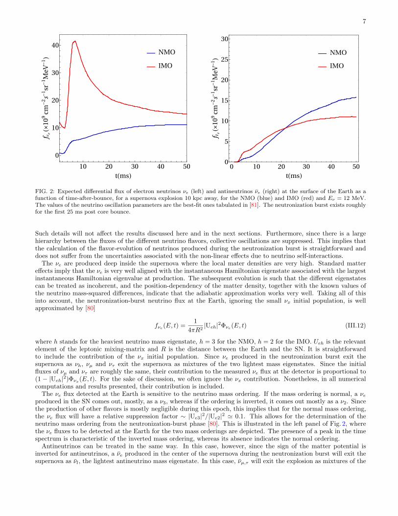
FIG. 2: Expected differential flux of electron neutrinos νe (left) and antineutrinos νe (right) at the surface of the Earth as afunction of time-after-bounce, for a supernova explosion 10 kpc away, for the NMO (blue) and IMO (red) and Eν = 12 MeV.The values of the neutrino oscillation parameters are the best-fit ones tabulated in [81]. The neutronization burst exists roughlyfor the first 25 ms post core bounce.

Such details will not affect the results discussed here and in the next sections. Furthermore, since there is a largehierarchy between the fluxes of the different neutrino flavors, collective oscillations are suppressed. This implies thatthe calculation of the flavor-evolution of neutrinos produced during the neutronization burst is straightforward anddoes not suffer from the uncertainties associated with the non-linear effects due to neutrino self-interactions.

The νe are produced deep inside the supernova where the local mater densities are very high. Standard mattereffects imply that the νe is very well aligned with the instantaneous Hamiltonian eigenstate associated with the largestinstantaneous Hamiltonian eigenvalue at production. The subsequent evolution is such that the different eigenstatescan be treated as incoherent, and the position-dependency of the matter density, together with the known values ofthe neutrino mass-squared differences, indicate that the adiabatic approximation works very well. Taking all of thisinto account, the neutronization-burst neutrino flux at the Earth, ignoring the small νx initial population, is wellapproximated by [80]

fνe(E, t) =1

4πR2|Ueh|2Φνe(E, t) (III.12)

where h stands for the heaviest neutrino mass eigenstate, h = 3 for the NMO, h = 2 for the IMO. Ueh is the relevantelement of the leptonic mixing-matrix and R is the distance between the Earth and the SN. It is straightforwardto include the contribution of the νx initial population. Since νe produced in the neutronization burst exit thesupernova as νh, νµ and ντ exit the supernova as mixtures of the two lightest mass eigenstates. Since the initialfluxes of νµ and ντ are roughly the same, their contribution to the measured νe flux at the detector is proportional to(1 − |Ueh|2)Φνx(E, t). For the sake of discussion, we often ignore the νx contribution. Nonetheless, in all numericalcomputations and results presented, their contribution is included.

The νe flux detected at the Earth is sensitive to the neutrino mass ordering. If the mass ordering is normal, a νeproduced in the SN comes out, mostly, as a ν3, whereas if the ordering is inverted, it comes out mostly as a ν2. Sincethe production of other flavors is mostly negligible during this epoch, this implies that for the normal mass ordering,the νe flux will have a relative suppression factor ∼ |Ue3|2/|Ue2|2 ' 0.1. This allows for the determination of theneutrino mass ordering from the neutronization-burst phase [80]. This is illustrated in the left panel of Fig. 2, wherethe νe fluxes to be detected at the Earth for the two mass orderings are depicted. The presence of a peak in the timespectrum is characteristic of the inverted mass ordering, whereas its absence indicates the normal ordering.

Antineutrinos can be treated in the same way. In this case, however, since the sign of the matter potential isinverted for antineutrinos, a νe produced in the center of the supernova during the neutronization burst will exit thesupernova as νl, the lightest antineutrino mass eigenstate. In this case, νµ,τ will exit the explosion as mixtures of the

8

two heaviest mass-eingenstates. The νe flux on Earth is depicted in the right panel of Fig. 2. Here, the distinctionbetween the two mass-orderings is a lot less pronounced. Nonetheless, it has been argued in the literature that therise time of the νe-flux can be exploited in very high statistics experiments, like IceCube [77, 82].

IV. IMPACT OF NEUTRINO DECAY ON THE NEUTRONIZATION-BURST FLUX

In this section, we outline the formalism for simulating the νe and the νe flux during the neutronization-burstepoch, incorporating both neutrino propagation and decay. The impact of neutrino decay on its propagation is givenby solving a transfer equation, which takes into account the decay of the heaviest-state population, as well as therepopulation of the lighter states [25]. The problem is simplified if we assume that the neutrinos do not decay withinthe SN envelope. Therefore, the neutronization-burst flux arrives unchanged at the surface of the SN, and decay ontheir way to the Earth. This is a good approximation as long as τ/m� 10−7s/eV.

The flux of a Dirac neutrino mass eigenstate i arriving at the Earth satisfies, for the ϕ0-model (Eq. (II.1)),

d

drfνi(E, r) = −Γνi→νj (E)fνi(E, r) +

∫ ∞E

dE′[ψh.c(E′, E)Γνj→νi(E

′)fνj (E′, r)

], (IV.13)

where ψh.c, ψh.f are defined in Eq. (II.3) and discussed in Section II. We have considered the fact that the daughter-neutrinos produced with the “wrong” helicity are effectively invisible. The first term accounts for the disappearanceof the parent-neutrinos while the second one accounts for the appearance of the daughters. The same equation, withν ↔ ν, holds for antineutrinos.

On the other hand, for the ϕ2-model (Eq. (II.4)),

d

drfνi(E, r) = −Γνi→νj (E)fνi(E, r) +

∫ ∞E

dE′[ψh.f(E

′, E)Γνj→νi(E′)fνj (E

′, r)].

d

drfνi(E, r) = −Γνi→νj (E)fνi(E, r) +

∫ ∞E

dE′[ψh.f(E

′, E)Γνj→νi(E′)fνj (E

′, r)]. (IV.14)

We have considered the fact that the daughter-(anti)neutrinos produced with the “same” helicity are effectivelyinvisible. Here, all neutrino decays lead to antineutrino daughters, hence all daughters are “lost.” On the other hand,the neutrino flux is replenished with daughters from parent-antineutrinos. For the neutronization burst, this is mostlyirrelevant for the νe detection on Earth but is very important for the νe signal.

In the case of Majorana neutrinos, taking advantage of the fact that the neutrino masses are much smaller than theneutrino energies in the lab frame, we can also define a “neutrino” and “antineutrino” flux. In this case, assumingthe decay scenario associated to Eq. (II.5),

d

drfνi(E, r) = −

(Γνi→νj (E) + Γνi→νj (E)

)fνi(E, r)

+

∫ ∞E

dE′[ψh.c(E′, E)Γνj→νi(E

′)fνj (E′, r) + ψh.f(E

′, E)Γνj→νi(E′)fνj (E

′, r)]

(IV.15)

The same equation holds also for antineutrinos with ν ↔ ν.Here, we focus on the situation where the heaviest mass eigenstate decays to the lightest one: in the NMO (IMO),

the ν3 (ν2) decays to a ν1 (ν3), leaving the intermediate mass-eigenstate – ν2 (ν1)– unchanged. There is no strongphysics argument in favor of this assumption, except that the effects are largest for these decay channels. Ourconclusions are mostly the same if one were to pursue the scenario where all allowed two-body decay modes of theheavier neutrinos are present.

Qualitatively, ignoring the relatively much smaller initial flux of νx and νe,x, this is what one expects of theneutronization-burst neutrino-flux if the neutrino lifetime is finite:

(a) For the NMO, Dirac neutrinos, and the ϕ0-model, the neutronization-burst neutrinos exit the supernova as ν3’s.The ν3 decays into visible and invisible ν1. While the daughter ν1 spectrum is softer than the one of the parent,the expected number of events may, in fact, be higher if the ν3 lifetime is short enough since |Ue3|2 � |Ue1|2. Itis possible to confuse this scenario with the IMO-case if the neutrino lifetime is chosen judiciously.

(b) For the IMO, Dirac neutrinos, and the ϕ0-model, the neutronization-burst neutrinos exit the supernova as ν2’s.The ν2 decays into visible and invisible ν3. The daughter ν3 spectrum is softer and |Ue3|2 � |Ue2|2 so one

9

expects a significant suppression of the neutronization-burst neutrino-flux. It is possible to confuse this scenariowith the NMO-case if the neutrino lifetime is chosen judiciously.

(c) For the NMO, Dirac neutrinos, and the ϕ2-model, the neutronization-burst neutrinos exit the supernova as ν3’s.The ν3 decays into visible and invisible ν1. The νe signal on the Earth is very small, but one anticipates ahealthy, softer νe signal.

(d) For the IMO, Dirac neutrinos, and the ϕ2-model, the neutronization-burst neutrinos exit the supernova as ν2’s.The ν2 decays into visible and invisible ν3. The νe signal on the Earth is suppressed due to the decay, and oneanticipates a small – |Ue3|2 � 1 – softer νe signal.

(e) For the NMO, Majorana neutrinos, and the model of interest here (Eq. (II.5)), the neutronization-burst neutrinosexit the supernova as ν3’s. The ν3 decays into visible ν1 and ν1 with different, softer spectra. Since |Ue3|2 �|Ue1|2, one may run into an excess of both νe and νe at Earth-bound detectors.

(f) For the IMO, Majorana neutrinos, and the model of interest here (Eq. (II.5)), the neutronization-burst neutrinosexit the supernova as ν2’s. The ν2 decays into visible ν3 and ν3 with different, softer spectra. Since |Ue3|2 �|Ue1|2, one expected a reduced number of νe and νe at Earth-bound detectors.

Note that, in general, we expect qualitatively different behaviors for the Dirac and Majorana decaying-neutrinoscenarios.

For the original νx spectrum, the impact of neutrino decay is absent for any mass-ordering since, in the regime ofinterest here, these always exit the supernova as a mixture of the lighter – assumed to be stable – mass eigenstates.For anti-neutrinos, the situation is reversed. An antineutrino born as a νe during the neutronization burst will exitthe supernova as the lightest antineutrino while half of the νx-born population will exit the supernova as the heaviestantineutrino and can hence subsequentially decay into ν1 (ν3) for the NMO (IMO).

We proceed to discuss more quantitatively the impact of neutrino decay in the measurement of neutrinos fromthe neutronization burst of the next galactic supernova assuming both the Deep Underground Neutrino Experiment(DUNE) and Hyper-KamiokaNDE (HK) are operational at the time of the momentous event. We first provide therelevant assumptions regarding our detection simulations.

V. SIMULATION DETAILS

We are interested in the future, very large neutrino detectors DUNE and HK, expected to come online in the middleof the next decade. The expected number of supernova neutrino events per unit time t and unit reconstructed energyEr at any detector is

d2N(Er, t)

dt dEr=

Ntg4πR2

∫dEtfνα(Et, t)σα(Et)ε(Et, Er), (V.16)

where fνα is the neutrino flux at the Earth, σα(E) is the relevant detection cross-section, and ε(Et, Er) is an energymigration matrix that relates the true neutrino energy Et to the reconstructed one. Ntg is the number of targets forthe experiment. We have assumed 40 ktons of liquid argon for DUNE and two water tanks of 187 ktons each for HK.R is the distance to the supernova. Unless otherwise noted, we have organized all simulated data into a 2-dimensionalarray of bins in energy and time. For the energy, we have considered a bin width of at least two times the detectorenergy resolution. For the time evolution are used 5 bins that account for the first 25 ms of the neutronization burst.

We have focused only on the dominant processes associated to the detection of supernova neutrinos at the twonext-generation experiments, described in more detail in what follows. DUNE is a liquid argon-based experiment[44], and we only consider the DUNE far detector given it will to be much larger than the near detector. For theenergies relevant to supernova neutrinos, DUNE is most sensitive to the νe component of the flux [83], measured viathe charged-current process

νe +40Ar→40K∗ + e−. (V.17)

The neutrino absorption by 40Ar creates an electron and an excited nucleus of potassium (40K∗) that will de-excite,producing a cascade of photons. The overall signal is characterized by a final state with several low-energy electro-magnetic tracks. In order to properly account for all of these, we make use of MARLEY [84], a Montecarlo eventgenerator that simulates νe interactions in Argon for energies less than 50 MeV. We use the simulated events toconstruct the energy migration matrix ε(Et, Er).

10

Liquid Argon experiments have proven the capability to observe electrons and photons in the MeV scale [85]. ForDUNE, we have assumed a minimum distance of 1.5 cm traveled by the electron in order to be detected; such distancetranslates into an energy threshold for the electron of 2 MeV. For photons, the dominant interaction at those energiesis Compton scattering and photons are observed as isolated blips near the electron track. We impose the same energycut in energy as the one for electrons. The reconstructed neutrino energy is the sum of the reconstructed energies for allthe final state particles, in our case electron and photons since the remaining recoiling nucleus cannot be observed. Theinteraction process proceed with an energy threshold of 4 MeV, which we consider as threshold for the reconstructedneutrino energy. The finite energy resolution of the detector introduces an error in the reconstruction of the neutrinoenergy. Assuming the same precision as shown in previous Liquid Argon experiments [86], we have included the energy

resolution via Montecarlo integration. The energy resolution increases as σE = 0.11√E/MeV + 0.2(E/MeV), and

corresponds to 5% for E ∼ 10 MeV. The time resolution for DUNE is expected to be of the order of ∼ 10 nsec [83].Since our simulated events are organized into time-bins of 5 ms, timing-resolution effects are irrelevant.

HK is a water Cherenkov detector. At the MeV scale, the main detection channel is inverse beta decay (IBD)(Eq. (V.18)), so HK is mainly sensitive to the electron-antineutrino component of the supernova neutrino flux:

νe + p→ e+ + n (V.18)

For the cross-section of IBD, we have used the results of the analytical calculation reported in Ref. [87], expected tobe valid for neutrino energies in the MeV to GeV range. Finally, we have assumed the energy resolution of HK to bethe same as that of Super-Kamiokande [73].‡ Considering σE = 0.6

√E/MeV, for an energy of 10 MeV, the energy

resolution is of the order of 20%. Note that for HK we are assuming a larger energy resolution which is translated intoa larger size of the energy bins. We have considered a threshold of 3 MeV in the energy measured, which is imposedby the detector capabilities to observe neutrinos [73]. To correlate the neutrino energy with the energy reconstructedby the detector, we made a Montecarlo integration assuming a Gaussian distribution of the energies measured by thedetector, where every event is weighted by the differential cross-section [87]. The time resolution for HK is of order5 nsec [73], negligible compared to our 5 ms time-bins.

In addition to IBD, the neutrino–electron scattering channel also contributes to the detection of SN neutrinos inHK. Given the large size of the detector, one can expect ∼ 23 (55) events for NMO (IMO) in one tank, for a SNoccuring at 10 kpc. This channel can, in principle, make it possible to observe the neutronization peak, if properbackground subtraction can be made. However, the neutrino–electron scattering channel is sensitive to neutrinos ofall flavors. Due to the difficulties in disentangling the νee scattering from the other neutrino flavors as well as theIBD events, we consider only the IBD channel for HK. The identification of the background via the neutron taggingby adding Gadolinium requires a more dedicated analysis, something that we will consider in future extensions of thiswork.

We make use of a χ2 analysis in order to compare different hypotheses and address different physics questions.We assume a Gaussian distribution for the χ2. For concreteness, the ∆χ2 for a set of values of the parameters givesus the significance over the test hypothesis. We bin our simulated events in energy and time, as discussed above,and marginalized over the different nuisance parameters in order to account for different systematic and statisticaleffects. For the remainder of this manuscript, unless otherwise noted, we assume that the overall normalization ofthe supernova neutrino flux is known at the 40% level (one sigma). For the neutrino mixing parameters, we use theresults of the global fit reported by the NuFit collaboration [81], and marginalize over the reported uncertainties forthe relevant mixing parameters – θ12 and θ13.

VI. IMPACT OF NEUTRINO DECAY AT DUNE AND HYPER-KAMIOKANDE

In this section, we explore some of the consequences of the neutrino decay hypothesis to future data from DUNE andHK. For concreteness, we concentrate on the hypothesis that the neutrinos are Dirac fermions and only the heaviestneutrino decays to the lightest neutrino. Therefore, in the NMO (IMO), the ν3 (ν2) decays to ν1 (ν3), similarly forantineutrinos. We will also concentrate on the ϕ0-model with gij = gji. Since we are assuming that DUNE is onlysensitive to the νe-component of the neutronization-burst neutrinos on Earth and HK is only sensitive to the νe-component, DUNE is expected to play a more significant role. It is clear from earlier discussions that the roles of thetwo detectors would be reversed in the ϕ2-model. Certain aspects of the hypothesis where the neutrinos are Majorana

‡ All of the results associated to HK also apply to Super-Kamiokande, currently taking data, once one takes into account the fact thatHK is expected to be an order of magnitude larger than Super-Kamiokande.

11

No Decay

τ/m=106 s/eV

τ/m=105 s/eV

τ/m=104 s/eV

0 5 10 15 20 250

20

40

60

80

100

120

t (ms)

Ev

en

tsDUNE

NMO No Decay

τ/m=106 s/eV

τ/m=105 s/eV

τ/m=104 s/eV

0 5 10 15 20 250

10

20

30

40

50

t (ms)

Ev

en

ts

DUNE

IMO

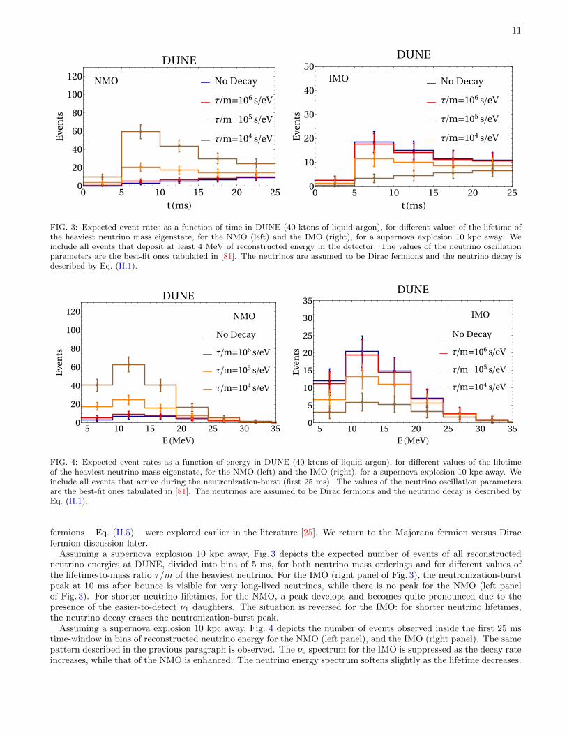
FIG. 3: Expected event rates as a function of time in DUNE (40 ktons of liquid argon), for different values of the lifetime ofthe heaviest neutrino mass eigenstate, for the NMO (left) and the IMO (right), for a supernova explosion 10 kpc away. Weinclude all events that deposit at least 4 MeV of reconstructed energy in the detector. The values of the neutrino oscillationparameters are the best-fit ones tabulated in [81]. The neutrinos are assumed to be Dirac fermions and the neutrino decay isdescribed by Eq. (II.1).

No Decay

τ/m=106 s/eV

τ/m=105 s/eV

τ/m=104 s/eV

5 10 15 20 25 30 350

20

40

60

80

100

120

E (MeV)

Ev

en

ts

DUNE

NMO

No Decay

τ/m=106 s/eV

τ/m=105 s/eV

τ/m=104 s/eV

5 10 15 20 25 30 350

5

10

15

20

25

30

35

E (MeV)

Ev

en

tsDUNE

IMO

FIG. 4: Expected event rates as a function of energy in DUNE (40 ktons of liquid argon), for different values of the lifetimeof the heaviest neutrino mass eigenstate, for the NMO (left) and the IMO (right), for a supernova explosion 10 kpc away. Weinclude all events that arrive during the neutronization-burst (first 25 ms). The values of the neutrino oscillation parametersare the best-fit ones tabulated in [81]. The neutrinos are assumed to be Dirac fermions and the neutrino decay is described byEq. (II.1).

fermions – Eq. (II.5) – were explored earlier in the literature [25]. We return to the Majorana fermion versus Diracfermion discussion later.

Assuming a supernova explosion 10 kpc away, Fig. 3 depicts the expected number of events of all reconstructedneutrino energies at DUNE, divided into bins of 5 ms, for both neutrino mass orderings and for different values ofthe lifetime-to-mass ratio τ/m of the heaviest neutrino. For the IMO (right panel of Fig. 3), the neutronization-burstpeak at 10 ms after bounce is visible for very long-lived neutrinos, while there is no peak for the NMO (left panelof Fig. 3). For shorter neutrino lifetimes, for the NMO, a peak develops and becomes quite pronounced due to thepresence of the easier-to-detect ν1 daughters. The situation is reversed for the IMO: for shorter neutrino lifetimes,the neutrino decay erases the neutronization-burst peak.

Assuming a supernova explosion 10 kpc away, Fig. 4 depicts the number of events observed inside the first 25 mstime-window in bins of reconstructed neutrino energy for the NMO (left panel), and the IMO (right panel). The samepattern described in the previous paragraph is observed. The νe spectrum for the IMO is suppressed as the decay rateincreases, while that of the NMO is enhanced. The neutrino energy spectrum softens slightly as the lifetime decreases.

12

3σ

3 4 5 6 7 8

50

10

5

1

log10τ/1 s

m/1 eV

Δχ

2

IMO vs NMO+Decay

1kpc

10kpc

50kpc

100kpc

FIG. 5:√

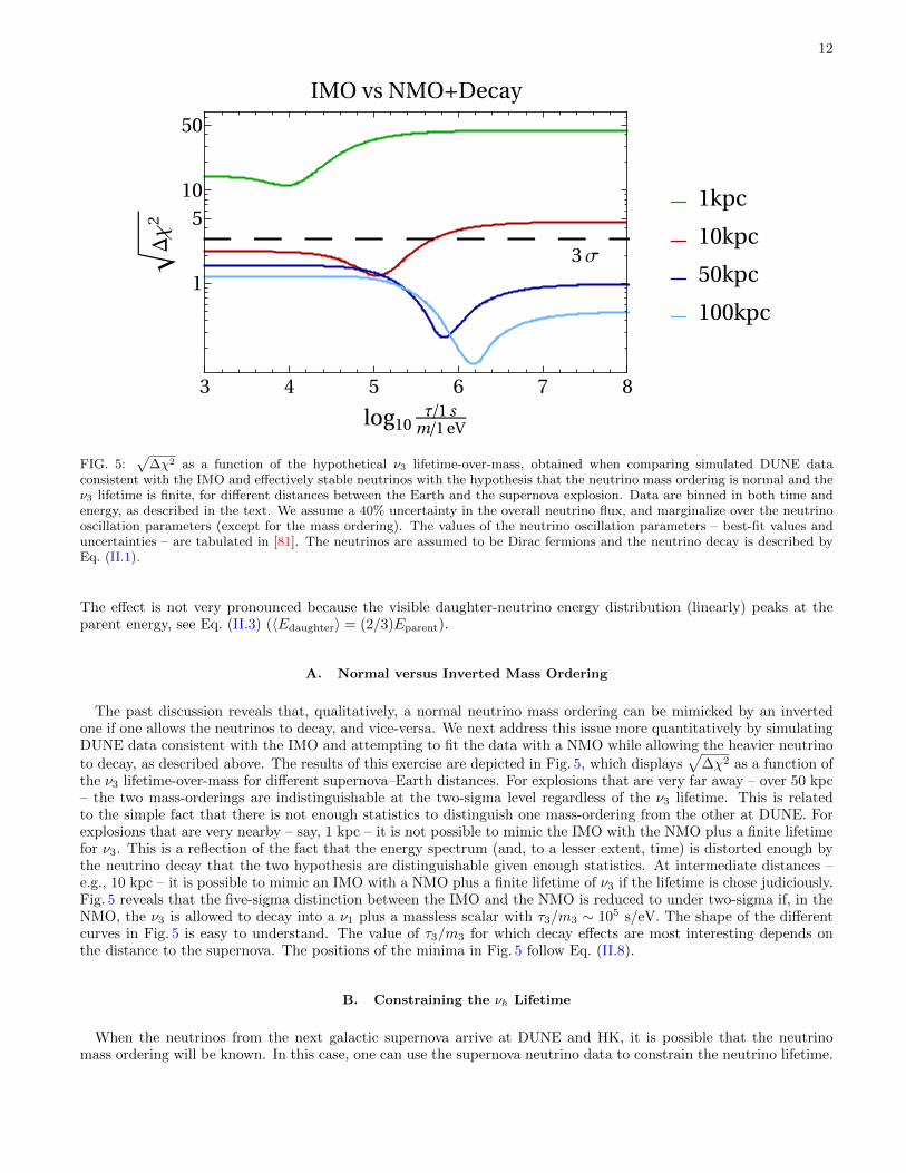
∆χ2 as a function of the hypothetical ν3 lifetime-over-mass, obtained when comparing simulated DUNE dataconsistent with the IMO and effectively stable neutrinos with the hypothesis that the neutrino mass ordering is normal and theν3 lifetime is finite, for different distances between the Earth and the supernova explosion. Data are binned in both time andenergy, as described in the text. We assume a 40% uncertainty in the overall neutrino flux, and marginalize over the neutrinooscillation parameters (except for the mass ordering). The values of the neutrino oscillation parameters – best-fit values anduncertainties – are tabulated in [81]. The neutrinos are assumed to be Dirac fermions and the neutrino decay is described byEq. (II.1).

The effect is not very pronounced because the visible daughter-neutrino energy distribution (linearly) peaks at theparent energy, see Eq. (II.3) (〈Edaughter〉 = (2/3)Eparent).

A. Normal versus Inverted Mass Ordering

The past discussion reveals that, qualitatively, a normal neutrino mass ordering can be mimicked by an invertedone if one allows the neutrinos to decay, and vice-versa. We next address this issue more quantitatively by simulatingDUNE data consistent with the IMO and attempting to fit the data with a NMO while allowing the heavier neutrino

to decay, as described above. The results of this exercise are depicted in Fig. 5, which displays√

∆χ2 as a function ofthe ν3 lifetime-over-mass for different supernova–Earth distances. For explosions that are very far away – over 50 kpc– the two mass-orderings are indistinguishable at the two-sigma level regardless of the ν3 lifetime. This is relatedto the simple fact that there is not enough statistics to distinguish one mass-ordering from the other at DUNE. Forexplosions that are very nearby – say, 1 kpc – it is not possible to mimic the IMO with the NMO plus a finite lifetimefor ν3. This is a reflection of the fact that the energy spectrum (and, to a lesser extent, time) is distorted enough bythe neutrino decay that the two hypothesis are distinguishable given enough statistics. At intermediate distances –e.g., 10 kpc – it is possible to mimic an IMO with a NMO plus a finite lifetime of ν3 if the lifetime is chose judiciously.Fig. 5 reveals that the five-sigma distinction between the IMO and the NMO is reduced to under two-sigma if, in theNMO, the ν3 is allowed to decay into a ν1 plus a massless scalar with τ3/m3 ∼ 105 s/eV. The shape of the differentcurves in Fig. 5 is easy to understand. The value of τ3/m3 for which decay effects are most interesting depends onthe distance to the supernova. The positions of the minima in Fig. 5 follow Eq. (II.8).

B. Constraining the νh Lifetime

When the neutrinos from the next galactic supernova arrive at DUNE and HK, it is possible that the neutrinomass ordering will be known. In this case, one can use the supernova neutrino data to constrain the neutrino lifetime.

13

SN

19

87

A

3σ

0 2 4 6 8

1

5

10

50

log10τ/1 s

m/1 eV

Δχ

2

Decay vs No Decay

NMO

1kpc

10kpc

50kpc

100kpc

FIG. 6:√

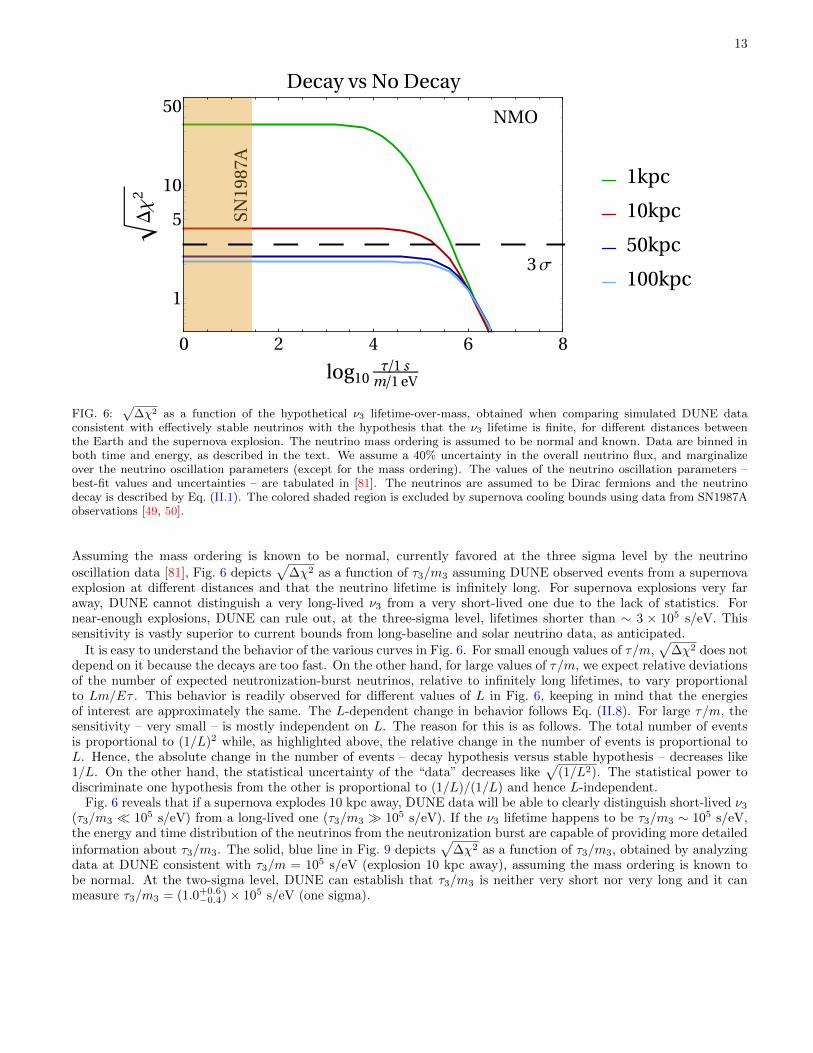
∆χ2 as a function of the hypothetical ν3 lifetime-over-mass, obtained when comparing simulated DUNE dataconsistent with effectively stable neutrinos with the hypothesis that the ν3 lifetime is finite, for different distances betweenthe Earth and the supernova explosion. The neutrino mass ordering is assumed to be normal and known. Data are binned inboth time and energy, as described in the text. We assume a 40% uncertainty in the overall neutrino flux, and marginalizeover the neutrino oscillation parameters (except for the mass ordering). The values of the neutrino oscillation parameters –best-fit values and uncertainties – are tabulated in [81]. The neutrinos are assumed to be Dirac fermions and the neutrinodecay is described by Eq. (II.1). The colored shaded region is excluded by supernova cooling bounds using data from SN1987Aobservations [49, 50].

Assuming the mass ordering is known to be normal, currently favored at the three sigma level by the neutrino

oscillation data [81], Fig. 6 depicts√

∆χ2 as a function of τ3/m3 assuming DUNE observed events from a supernovaexplosion at different distances and that the neutrino lifetime is infinitely long. For supernova explosions very faraway, DUNE cannot distinguish a very long-lived ν3 from a very short-lived one due to the lack of statistics. Fornear-enough explosions, DUNE can rule out, at the three-sigma level, lifetimes shorter than ∼ 3 × 105 s/eV. Thissensitivity is vastly superior to current bounds from long-baseline and solar neutrino data, as anticipated.

It is easy to understand the behavior of the various curves in Fig. 6. For small enough values of τ/m,√

∆χ2 does notdepend on it because the decays are too fast. On the other hand, for large values of τ/m, we expect relative deviationsof the number of expected neutronization-burst neutrinos, relative to infinitely long lifetimes, to vary proportionalto Lm/Eτ . This behavior is readily observed for different values of L in Fig. 6, keeping in mind that the energiesof interest are approximately the same. The L-dependent change in behavior follows Eq. (II.8). For large τ/m, thesensitivity – very small – is mostly independent on L. The reason for this is as follows. The total number of eventsis proportional to (1/L)2 while, as highlighted above, the relative change in the number of events is proportional toL. Hence, the absolute change in the number of events – decay hypothesis versus stable hypothesis – decreases like1/L. On the other hand, the statistical uncertainty of the “data” decreases like

√(1/L2). The statistical power to

discriminate one hypothesis from the other is proportional to (1/L)/(1/L) and hence L-independent.Fig. 6 reveals that if a supernova explodes 10 kpc away, DUNE data will be able to clearly distinguish short-lived ν3

(τ3/m3 � 105 s/eV) from a long-lived one (τ3/m3 � 105 s/eV). If the ν3 lifetime happens to be τ3/m3 ∼ 105 s/eV,the energy and time distribution of the neutrinos from the neutronization burst are capable of providing more detailed

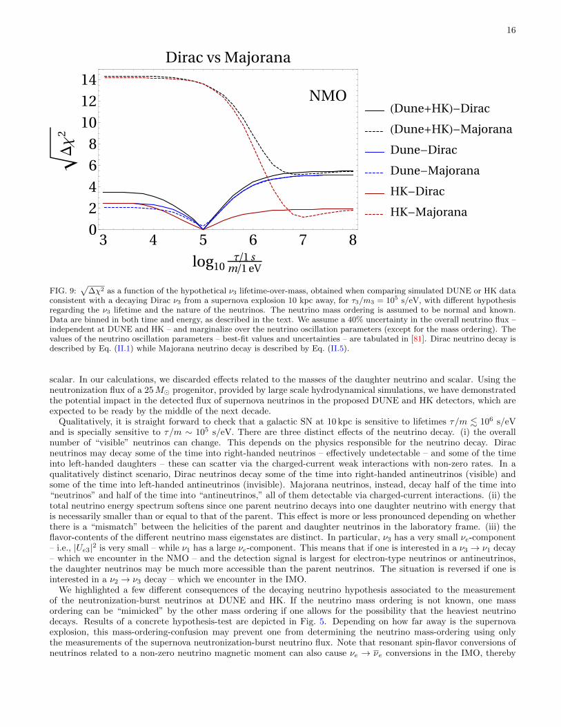
information about τ3/m3. The solid, blue line in Fig. 9 depicts√

∆χ2 as a function of τ3/m3, obtained by analyzingdata at DUNE consistent with τ3/m = 105 s/eV (explosion 10 kpc away), assuming the mass ordering is known tobe normal. At the two-sigma level, DUNE can establish that τ3/m3 is neither very short nor very long and it canmeasure τ3/m3 = (1.0+0.6

−0.4)× 105 s/eV (one sigma).

14

Dirac

Majorana

0 5 10 15 20 250

10

20

30

40

t (ms)

Ev

en

tsDUNE

NMO

τ/m=105 s/eV

Dirac

Majorana

0 5 10 15 20 250

100

200

300

400

500

t (ms)

Ev

en

ts

Hyper-K

NMO

τ/m=105 s/eV

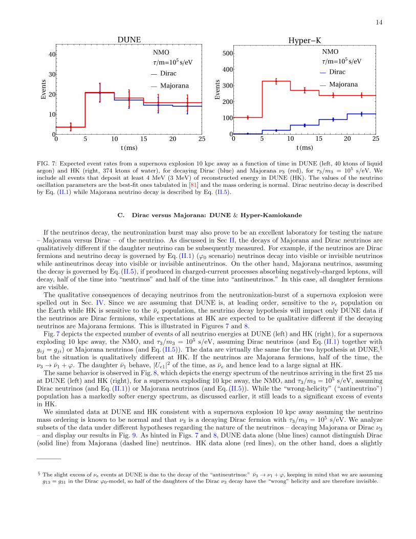
FIG. 7: Expected event rates from a supernova explosion 10 kpc away as a function of time in DUNE (left, 40 ktons of liquidargon) and HK (right, 374 ktons of water), for decaying Dirac (blue) and Majorana ν3 (red), for τ3/m3 = 105 s/eV. Weinclude all events that deposit at least 4 MeV (3 MeV) of reconstructed energy in DUNE (HK). The values of the neutrinooscillation parameters are the best-fit ones tabulated in [81] and the mass ordering is normal. Dirac neutrino decay is describedby Eq. (II.1) while Majorana neutrino decay is described by Eq. (II.5).

C. Dirac versus Majorana: DUNE & Hyper-Kamiokande

If the neutrinos decay, the neutronization burst may also prove to be an excellent laboratory for testing the nature– Majorana versus Dirac – of the neutrino. As discussed in Sec II, the decays of Majorana and Dirac neutrinos arequalitatively different if the daughter neutrino can be subsequently measured. For example, if the neutrinos are Diracfermions and neutrino decay is governed by Eq. (II.1) (ϕ0 scenario) neutrinos decay into visible or invisible neutrinoswhile antineutrinos decay into visible or invisible antineutrinos. On the other hand, Majorana neutrinos, assumingthe decay is governed by Eq. (II.5), if produced in charged-current processes absorbing negatively-charged leptons, willdecay, half of the time into “neutrinos” and half of the time into “antineutrinos.” In this case, all daughter fermionsare visible.

The qualitative consequences of decaying neutrinos from the neutronization-burst of a supernova explosion werespelled out in Sec. IV. Since we are assuming that DUNE is, at leading order, sensitive to the νe population onthe Earth while HK is sensitive to the νe population, the neutrino decay hypothesis will impact only DUNE data ifthe neutrinos are Dirac fermions, while expectations at HK are expected to be qualitative different if the decayingneutrinos are Majorana fermions. This is illustrated in Figures 7 and 8.

Fig. 7 depicts the expected number of events of all neutrino energies at DUNE (left) and HK (right), for a supernovaexploding 10 kpc away, the NMO, and τ3/m3 = 105 s/eV, assuming Dirac neutrinos (and Eq. (II.1) together withgij = gji) or Majorana neutrinos (and Eq. (II.5)). The data are virtually the same for the two hypothesis at DUNE,§

but the situation is qualitatively different at HK. If the neutrinos are Majorana fermions, half of the time, theν3 → ν1 + ϕ. The daughter ν1 behave, |Ue1|2 of the time, as νe and hence lead to a large signal at HK.

The same behavior is observed in Fig. 8, which depicts the energy spectrum of the neutrinos arriving in the first 25 msat DUNE (left) and HK (right), for a supernova exploding 10 kpc away, the NMO, and τ3/m3 = 105 s/eV, assumingDirac neutrinos (and Eq. (II.1)) or Majorana neutrinos (and Eq. (II.5)). While the “wrong-helicity” (“antineutrino”)population has a markedly softer energy spectrum, as discussed earlier, it still leads to a significant excess of eventsin HK.

We simulated data at DUNE and HK consistent with a supernova explosion 10 kpc away assuming the neutrinomass ordering is known to be normal and that ν3 is a decaying Dirac fermion with τ3/m3 = 105 s/eV. We analyzesubsets of the data under different hypotheses regarding the nature of the neutrinos – decaying Majorana or Dirac ν3

– and display our results in Fig. 9. As hinted in Figs. 7 and 8, DUNE data alone (blue lines) cannot distinguish Dirac(solid line) from Majorana (dashed line) neutrinos. HK data alone (red lines), on the other hand, does a slightly

§ The slight excess of νe events at DUNE is due to the decay of the “antineutrinos:” ν3 → ν1 + ϕ, keeping in mind that we are assumingg13 = g31 in the Dirac ϕ0-model, so half of the daughters of the Dirac ν3 decay have the “wrong” helicity and are therefore invisible.

15

Dirac

Majorana

10 20 30 40 500

10

20

30

40

E (MeV)

Ev

en

tsDUNE

NMO

τ/m=105 s/eV

Dirac

Majorana

10 20 30 40 500

100

200

300

400

500

600

E (MeV)

Ev

en

ts

Hyper-K

NMO

τ/m=105 s/eV

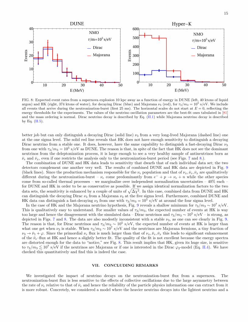
FIG. 8: Expected event rates from a supernova explosion 10 kpc away as a function of energy in DUNE (left, 40 ktons of liquidargon) and HK (right, 374 ktons of water), for decaying Dirac (blue) and Majorana ν3 (red), for τ3/m3 = 105 s/eV. We includeall events that arrive during the neutronization-burst (first 25 ms). The horizontal scales do not start at E = 0, reflecting theenergy thresholds for the experiments. The values of the neutrino oscillation parameters are the best-fit ones tabulated in [81]and the mass ordering is normal. Dirac neutrino decay is described by Eq. (II.1) while Majorana neutrino decay is describedby Eq. (II.5).

better job but can only distinguish a decaying Dirac (solid line) ν3 from a very long-lived Majorana (dashed line) oneat the one sigma level. The solid red line reveals that HK does not have enough sensitivity to distinguish a decayingDirac neutrino from a stable one. It does, however, have the same capability to distinguish a fast-decaying Dirac ν3

from one with τ3/m3 = 105 s/eV as DUNE. The reason is that, in spite of the fact that HK does not see the dominantneutrinos from the deleptonization process, it is large enough to see a very healthy sample of antineutrinos born asνe and νx, even if one restricts the analysis only to the neutronization-burst period (see Figs. 7 and 8.).

The combination of DUNE and HK data leads to sensitivity that dwarfs that of each individual data set; the twodetectors complement one another very well. The results of combined DUNE and HK data are depicted in Fig. 9(black lines). Since the production mechanism responsible for the νe population and that of νx, νe, νx are qualitativelydifferent during the neutronization-burst – νe come predominantly from e− + p → νe + n while the other speciescome from so-called thermal processes – we marginalize over independent normalization uncertainties – 40% each –for DUNE and HK in order to be as conservative as possible. If we assign identical normalization factors to the two

data sets, the sensitivity is enhanced by a couple of units of√

∆χ2. In this case, combined data from DUNE and HKcan distinguish the decaying Dirac ν3 from a Majorana ν3 at the five sigma level. Furthermore, combined DUNE andHK data can distinguish a fast-decaying ν3 from one with τ3/m3 = 105 s/eV at around the four sigma level.

In the case of HK and the Majorana neutrino hypothesis, Fig. 9 reveals a shallow minimum for τ3/m3 ∼ 107 s/eV.This is qualitatively easy to understand. For smaller values of τ3/m3, the expected number of events at HK is waytoo large and hence the disagreement with the simulated data – Dirac neutrinos and τ3/m3 ∼ 105 s/eV – is strong, asdepicted in Figs. 7 and 8. The data are also modestly inconsistent with a stable ν3, as one can see clearly in Fig. 9.The reason is that, for Dirac neutrinos and τ3/m3 ∼ 105 s/eV, the expected number of events at HK is larger thanwhat one get when ν3 is stable. When τ3/m3 ∼ 107 s/eV and the neutrinos are Majorana fermions, a tiny fraction ofν3 → ν1 + ϕ. Since the primordial νe flux is much larger than that of νx, νe, νx this leads to significant enhancementof the νe–flux at HK and hence a slightly better fit. The quality of the fit is not excellent because the energy spectraare distorted enough for the data to “notice,” see Fig. 8. This result implies that HK, given its huge size, is sensitiveto τ3/m3 . 107 s/eV if the neutrinos are Majorana or if one is interested in the Dirac ϕ2-model (Eq. II.4). We havechecked this quantitatively and find this is indeed the case.

VII. CONCLUDING REMARKS

We investigated the impact of neutrino decays on the neutronization-burst flux from a supernova. Theneutronization-burst flux is less sensitive to the effects of collective oscillations due to the large asymmetry betweenthe rate of νe relative to that of νe and hence the reliability of the particle physics information one can extract from itis more robust. Concretely, we considered a model where the heavier neutrino decays into the lightest neutrino and a

16

3 4 5 6 7 80

2

4

6

8

10

12

14

log10τ/1 s

m/1 eV

Δχ

2Dirac vs Majorana

NMO(Dune+HK)-Dirac

(Dune+HK)-Majorana

Dune-Dirac

Dune-Majorana

HK-Dirac

HK-Majorana

FIG. 9:√

∆χ2 as a function of the hypothetical ν3 lifetime-over-mass, obtained when comparing simulated DUNE or HK dataconsistent with a decaying Dirac ν3 from a supernova explosion 10 kpc away, for τ3/m3 = 105 s/eV, with different hypothesisregarding the ν3 lifetime and the nature of the neutrinos. The neutrino mass ordering is assumed to be normal and known.Data are binned in both time and energy, as described in the text. We assume a 40% uncertainty in the overall neutrino flux –independent at DUNE and HK – and marginalize over the neutrino oscillation parameters (except for the mass ordering). Thevalues of the neutrino oscillation parameters – best-fit values and uncertainties – are tabulated in [81]. Dirac neutrino decay isdescribed by Eq. (II.1) while Majorana neutrino decay is described by Eq. (II.5).

scalar. In our calculations, we discarded effects related to the masses of the daughter neutrino and scalar. Using theneutronization flux of a 25M� progenitor, provided by large scale hydrodynamical simulations, we have demonstratedthe potential impact in the detected flux of supernova neutrinos in the proposed DUNE and HK detectors, which areexpected to be ready by the middle of the next decade.

Qualitatively, it is straight forward to check that a galactic SN at 10 kpc is sensitive to lifetimes τ/m . 106 s/eVand is specially sensitive to τ/m ∼ 105 s/eV. There are three distinct effects of the neutrino decay. (i) the overallnumber of “visible” neutrinos can change. This depends on the physics responsible for the neutrino decay. Diracneutrinos may decay some of the time into right-handed neutrinos – effectively undetectable – and some of the timeinto left-handed daughters – these can scatter via the charged-current weak interactions with non-zero rates. In aqualitatively distinct scenario, Dirac neutrinos decay some of the time into right-handed antineutrinos (visible) andsome of the time into left-handed antineutrinos (invisible). Majorana neutrinos, instead, decay half of the time into“neutrinos” and half of the time into “antineutrinos,” all of them detectable via charged-current interactions. (ii) thetotal neutrino energy spectrum softens since one parent neutrino decays into one daughter neutrino with energy thatis necessarily smaller than or equal to that of the parent. This effect is more or less pronounced depending on whetherthere is a “mismatch” between the helicities of the parent and daughter neutrinos in the laboratory frame. (iii) theflavor-contents of the different neutrino mass eigenstates are distinct. In particular, ν3 has a very small νe-component– i.e., |Ue3|2 is very small – while ν1 has a large νe-component. This means that if one is interested in a ν3 → ν1 decay– which we encounter in the NMO – and the detection signal is largest for electron-type neutrinos or antineutrinos,the daughter neutrinos may be much more accessible than the parent neutrinos. The situation is reversed if one isinterested in a ν2 → ν3 decay – which we encounter in the IMO.

We highlighted a few different consequences of the decaying neutrino hypothesis associated to the measurementof the neutronization-burst neutrinos at DUNE and HK. If the neutrino mass ordering is not known, one massordering can be “mimicked” by the other mass ordering if one allows for the possibility that the heaviest neutrinodecays. Results of a concrete hypothesis-test are depicted in Fig. 5. Depending on how far away is the supernovaexplosion, this mass-ordering-confusion may prevent one from determining the neutrino mass-ordering using onlythe measurements of the supernova neutronization-burst neutrino flux. Note that resonant spin-flavor conversions ofneutrinos related to a non-zero neutrino magnetic moment can also cause νe → νe conversions in the IMO, thereby

17

resulting in a vanishing neutronization peak. This scenario, however, requires very strong magnetic fields inside theSN ∼ O(1010) G or larger [88, 89].

On the other hand, if the neutrino mass-ordering is known, measurements of the supernova neutronization-burstneutrino flux allow one to constrain the neutrino lifetime. If data at DUNE are consistent with stable neutrinos, Fig. 6reveals that, for a specific model (Dirac neutrinos, ϕ0-scenario), τ/m values less than 105 s/eV can be safely ruled outif the supernova explosion is not too far away. This sensitivity is far superior to that of solar-system-bound oscillationexperiments, by many orders of magnitude (10−3 s/eV versus 105 s/eV). In other scenarios (e.g., Dirac neutrinos andthe ϕ2-scenario or Majorana neutrinos), introduced here but not explored in great detail in the preceding sections,HK is expected to provide most of the sensitivity. Improvements in the background identification in HK by neutrontagging, which will make it sensitive to the Dirac ϕ0-scenario, will be considered in future extensions of the work.We have computed the equivalent of Fig. 6 assuming the neutrinos are Majorana fermions and concentrating on HKdata. We find that, for a SN 10 kpc away, HK can rule out τ/m values less than 107 s/eV, which corresponds to acoupling |g| & 2.3× 10−10.

Stronger bounds than the sensitivities discussed here can be extracted from the properties of the cosmic neutrinobackground, indirectly constrained by cosmic surveys of different types. Precise measurements of the cosmic microwavebackground from Planck 2015 constrain the neutrino free-streaming length and hence limit the strength of neutrino–neutrino interactions, including those mediated by the light scalars ϕ introduced here. These constraints can betranslated into very strong constraints on the neutrino lifetime τν > 4×108 s (mν/0.05 eV)3 for SM neutrinos decayinginto lighter neutrinos and dark radiation [90] . These and other cosmological bounds, however, are indirect probes ofneutrino decay. We advocate that such bounds are qualitatively distinct and that more direct bounds from “terrestrial”experiments complement the more indirect results from cosmic surveys.

We emphasized the fact that decaying Majorana and Dirac neutrinos are qualitatively different and potentiallyeasy to distinguish. Qualitatively, the most relevant feature is that, in general, Dirac neutrinos decay either intoneutrinos or antineutrinos while Majorana neutrinos decay into both neutrinos and antineutrinos. We showed that,by combining data from DUNE (sensitive to νe) and HK (sensitive to νe) one should be able to distinguish a decayingDirac neutrino from a Majorana one. The results of a concrete exercise are depicted in Fig. 9. The complementarityof the two next-generation experiment is quite apparent. We re-emphasize, however, that it is always possible toconcoct different models where one cannot distinguish Majorana from Dirac decaying neutrinos, as we discuss in somedetail in Sec. IIC.

We restricted most of our discussion to one of the models introduced in Sec. II, the ϕ0-model, with gij = gji,described in Eq. (II.1). Many of the results discussed here would also apply in the ϕ2-model and in the case whereneutrinos are Majorana fermions. In these other scenarios, however, the relative role of DUNE and HK data maybe quite distinct. While we concentrated on the decay of neutrinos into other neutrinos and a new scalar particle,there are many other possibilities. In the absence of no new light degrees of freedom the neutrino three-body decays(νh → νlν

′lν′′l ) could lead to some of the same effects discussed here. We plan to return to these decay modes in

future work. More very large neutrino experiments, other than DUNE and HK, are expected to be on-line in thelatter half of the next decade, including IceCube (ice), KM3Net (salt water), JUNO (liquid scintillator), etc. We didnot consider the impact of their data in our many analyses. For example, the large volume and the time resolutionof IceCube [91] have been already exploited in determining the rise time of the νe flux during the neutronizationburst. The helicity-flipping decays of heavier neutrinos during this epoch could lead to the identification of a peak atIceCube. However, the uncertainties in the background and the determination of the onset of the signal, as well asthe difficulties in the reconstruction of the neutrino energy, will negatively impact the IceCube sensitivity. We planto return to these and related issues in the future.

Acknowledgements

We would like to thank Edoardo Vitagliano for useful discussions. The work of AdG was supported in part by DOEgrant #DE-SC0010143. IMS acknowledges travel support from the Colegio de Fısica Fundamental e Interdisciplinariade las Americas (COFI). MS acknowledges support from the National Science Foundation, Grant PHY-1630782, andto the Heising-Simons Foundation, Grant 2017-228. Fermilab is operated by the Fermi Research Alliance, LLC undercontract No. DE-AC02-07CH11359 with the United States Department of Energy.

[1] Particle Data Group Collaboration, M. Tanabashi et al., “Review of Particle Physics”, Phys. Rev. D98 (2018), no. 3,030001.

18

[2] J. N. Bahcall, N. Cabibbo, and A. Yahil, “Are neutrinos stable particles?”, Phys. Rev. Lett. 28 (1972) 316–318,[,285(1972)].

[3] J. Schechter and J. W. F. Valle, “Neutrino Decay and Spontaneous Violation of Lepton Number”, Phys. Rev. D25(1982) 774.

[4] J. N. Bahcall, S. T. Petcov, S. Toshev, and J. W. F. Valle, “Tests of Neutrino Stability”, Phys. Lett. B181 (1986)369–374.

[5] S. Nussinov, “Some Comments on Decaying Neutrinos and the Triplet Majoron Model”, Phys. Lett. B185 (1987)171–176.

[6] J. A. Frieman, H. E. Haber, and K. Freese, “Neutrino Mixing, Decays and Supernova Sn1987a”, Phys. Lett. B200 (1988)115–121.

[7] C. W. Kim and W. P. Lam, “Some remarks on neutrino decay via a Nambu-Goldstone boson”, Mod. Phys. Lett. A5(1990) 297–299.

[8] S. D. Biller et al., “New limits to the IR background: Bounds on radiative neutrino decay and on VMO contributions tothe dark matter problem”, Phys. Rev. Lett. 80 (1998) 2992–2995, arXiv:astro-ph/9802234.

[9] Y. Chikashige, R. N. Mohapatra, and R. D. Peccei, “Spontaneously broken lepton number and cosmological constraintson the neutrino mass spectrum”, Phys. Rev. Lett. 45 Dec (1980) 1926–1929.

[10] G. Gelmini and M. Roncadelli, “Left-handed neutrino mass scale and spontaneously broken lepton number”, PhysicsLetters B 99 (1981), no. 5, 411 – 415.

[11] G. B. Gelmini and J. W. F. Valle, “Fast Invisible Neutrino Decays”, Phys. Lett. 142B (1984) 181–187.[12] S. Bertolini and A. Santamaria, “The doublet majoron model and solar neutrino oscillations”, Nuclear Physics B 310

(1988), no. 3, 714 – 742.[13] A. Santamaria and J. Valle, “Spontaneous r parity violation in supersymmetry: A model for solar neutrino oscillations”,

Physics Letters B 195 (1987), no. 3, 423 – 428.[14] J. F. Beacom and N. F. Bell, “Do solar neutrinos decay?”, Phys. Rev. D65 (2002) 113009, arXiv:hep-ph/0204111.[15] P. Coloma and O. L. G. Peres, “Visible neutrino decay at DUNE”, arXiv:1705.03599.[16] A. B. Balantekin, A. de Gouvea, and B. Kayser, “Addressing the Majorana vs. Dirac Question with Neutrino Decays”,

Phys. Lett. B789 (2019) 488–495, arXiv:1808.10518.[17] L. Funcke, G. Raffelt, and E. Vitagliano, “Distinguishing Dirac and Majorana neutrinos by their gravi-majoron decays”,

arXiv:1905.01264.[18] Z. G. Berezhiani, G. Fiorentini, M. Moretti, and A. Rossi, “Fast neutrino decay and solar neutrino detectors”, Zeitschrift

fur Physik C Particles and Fields 54 Dec (1992) 581–586.[19] G. L. Fogli, E. Lisi, A. Marrone, and G. Scioscia, “Super-Kamiokande data and atmospheric neutrino decay”, Phys. Rev.

D59 (1999) 117303, arXiv:hep-ph/9902267.[20] S. Choubey, S. Goswami, and D. Majumdar, “Status of the neutrino decay solution to the solar neutrino problem”, Phys.

Lett. B484 (2000) 73–78, arXiv:hep-ph/0004193.[21] M. Lindner, T. Ohlsson, and W. Winter, “A Combined treatment of neutrino decay and neutrino oscillations”, Nucl.

Phys. B607 (2001) 326–354, arXiv:hep-ph/0103170.[22] A. S. Joshipura, E. Masso, and S. Mohanty, “Constraints on decay plus oscillation solutions of the solar neutrino

problem”, Phys. Rev. D66 (2002) 113008, arXiv:hep-ph/0203181.[23] A. Bandyopadhyay, S. Choubey, and S. Goswami, “Neutrino decay confronts the SNO data”, Phys. Lett. B555 (2003)

33–42, arXiv:hep-ph/0204173.[24] S. Ando, “Decaying neutrinos and implications from the supernova relic neutrino observation”, Phys. Lett. B570 (2003)

11, arXiv:hep-ph/0307169.[25] S. Ando, “Appearance of neutronization peak and decaying supernova neutrinos”, Phys. Rev. D70 (2004) 033004,

arXiv:hep-ph/0405200.[26] J. F. Beacom, N. F. Bell, and S. Dodelson, “Neutrinoless universe”, Phys. Rev. Lett. 93 (2004) 121302,

arXiv:astro-ph/0404585.[27] J. M. Berryman, A. de Gouvea, and D. Hernandez, “Solar Neutrinos and the Decaying Neutrino Hypothesis”, Phys. Rev.

D92 (2015), no. 7, 073003, arXiv:1411.0308.[28] R. Picoreti, M. M. Guzzo, P. C. de Holanda, and O. L. G. Peres, “Neutrino Decay and Solar Neutrino Seasonal Effect”,

Phys. Lett. B761 (2016) 70–73, arXiv:1506.08158.[29] J. A. Frieman, H. E. Haber, and K. Freese, “Neutrino mixing, decays and supernova 1987a”, Physics Letters B 200

(1988), no. 1, 115 – 121.[30] A. Mirizzi, D. Montanino, and P. D. Serpico, “Revisiting cosmological bounds on radiative neutrino lifetime”, Phys. Rev.

D76 (2007) 053007, arXiv:0705.4667.[31] M. C. Gonzalez-Garcia and M. Maltoni, “Status of Oscillation plus Decay of Atmospheric and Long-Baseline Neutrinos”,

Phys. Lett. B663 (2008) 405–409, arXiv:0802.3699.[32] M. Maltoni and W. Winter, “Testing neutrino oscillations plus decay with neutrino telescopes”, JHEP 07 (2008) 064,

arXiv:0803.2050.[33] P. Baerwald, M. Bustamante, and W. Winter, “Neutrino Decays over Cosmological Distances and the Implications for

Neutrino Telescopes”, JCAP 1210 (2012) 020, arXiv:1208.4600.[34] C. Broggini, C. Giunti, and A. Studenikin, “Electromagnetic Properties of Neutrinos”, Adv. High Energy Phys. 2012

(2012) 459526, arXiv:1207.3980.[35] L. Dorame, O. G. Miranda, and J. W. F. Valle, “Invisible decays of ultra-high energy neutrinos”, Front.in Phys. 1 (2013)

19

25, arXiv:1303.4891.[36] R. A. Gomes, A. L. G. Gomes, and O. L. G. Peres, “Constraints on neutrino decay lifetime using long-baseline charged

and neutral current data”, Phys. Lett. B740 (2015) 345–352, arXiv:1407.5640.[37] T. Abrahao, H. Minakata, H. Nunokawa, and A. A. Quiroga, “Constraint on Neutrino Decay with Medium-Baseline

Reactor Neutrino Oscillation Experiments”, JHEP 11 (2015) 001, arXiv:1506.02314.[38] A. M. Gago, R. A. Gomes, A. L. G. Gomes, J. Jones-Perez, and O. L. G. Peres, “Visible neutrino decay in the light of

appearance and disappearance long baseline experiments”, JHEP 11 (2017) 022, arXiv:1705.03074.[39] S. Choubey, D. Dutta, and D. Pramanik, “Invisible neutrino decay in the light of NOvA and T2K data”, JHEP 08

(2018) 141, arXiv:1805.01848.[40] P. F. de Salas, S. Pastor, C. A. Ternes, T. Thakore, and M. Tortola, “Constraining the invisible neutrino decay with

KM3NeT-ORCA”, Phys. Lett. B789 (2019) 472–479, arXiv:1810.10916.[41] BOREXINO Collaboration, G. Bellini et al., “Neutrinos from the primary proton–proton fusion process in the Sun”,

Nature 512 (2014), no. 7515, 383–386.[42] SNO Collaboration, B. Aharmim et al., “Constraints on Neutrino Lifetime from the Sudbury Neutrino Observatory”,

Phys. Rev. D99 (2019), no. 3, 032013, arXiv:1812.01088.[43] JUNO Collaboration, F. An et al., “Neutrino Physics with JUNO”, J. Phys. G43 (2016), no. 3, 030401,

arXiv:1507.05613.[44] DUNE Collaboration, R. Acciarri et al., “Long-Baseline Neutrino Facility (LBNF) and Deep Underground Neutrino

Experiment (DUNE)”, arXiv:1601.05471.[45] K. Hirata, T. Kajita, M. Koshiba, M. Nakahata, Y. Oyama, N. Sato, A. Suzuki, M. Takita, Y. Totsuka, T. Kifune,

T. Suda, K. Takahashi, T. Tanimori, K. Miyano, M. Yamada, E. W. Beier, L. R. Feldscher, S. B. Kim, A. K. Mann,F. M. Newcomer, R. Van, W. Zhang, and B. G. Cortez, “Observation of a neutrino burst from the supernova sn1987a”,Phys. Rev. Lett. 58 Apr (1987) 1490–1493.

[46] R. M. Bionta, G. Blewitt, C. B. Bratton, D. Casper, A. Ciocio, R. Claus, B. Cortez, M. Crouch, S. T. Dye, S. Errede,G. W. Foster, W. Gajewski, K. S. Ganezer, M. Goldhaber, T. J. Haines, T. W. Jones, D. Kielczewska, W. R. Kropp,J. G. Learned, J. M. LoSecco, J. Matthews, R. Miller, M. S. Mudan, H. S. Park, L. R. Price, F. Reines, J. Schultz,S. Seidel, E. Shumard, D. Sinclair, H. W. Sobel, J. L. Stone, L. R. Sulak, R. Svoboda, G. Thornton, J. C. van der Velde,and C. Wuest, “Observation of a neutrino burst in coincidence with supernova 1987a in the large magellanic cloud”,Phys. Rev. Lett. 58 Apr (1987) 1494–1496.

[47] G. M. Fuller, R. Mayle, and J. R. Wilson, “The Majoron Model and Stellar Collapse”, Astrophys. J. 332 Sep (1988) 826.[48] Z. G. Berezhiani and A. Yu. Smirnov, “Matter Induced Neutrino Decay and Supernova SN1987A”, Phys. Lett. B220

(1989) 279–284.[49] M. Kachelriess, R. Tomas, and J. W. F. Valle, “Supernova bounds on Majoron emitting decays of light neutrinos”, Phys.

Rev. D62 (2000) 023004, arXiv:hep-ph/0001039.[50] Y. Farzan, “Bounds on the coupling of the Majoron to light neutrinos from supernova cooling”, Phys. Rev. D67 (2003)

073015, arXiv:hep-ph/0211375.[51] IceCube Collaboration, M. G. Aartsen et al., “Observation of High-Energy Astrophysical Neutrinos in Three Years of

IceCube Data”, Phys. Rev. Lett. 113 (2014) 101101, arXiv:1405.5303.[52] P. B. Denton and I. Tamborra, “Invisible Neutrino Decay Could Resolve IceCube’s Track and Cascade Tension”, Phys.

Rev. Lett. 121 (2018), no. 12, 121802, arXiv:1805.05950.[53] L. Oberauer, C. Hagner, G. Raffelt, and E. Rieger, “Supernova bounds on neutrino radiative decays”, Astroparticle

Physics 1 (1993) 377–386.[54] J. F. Beacom, N. F. Bell, D. Hooper, S. Pakvasa, and T. J. Weiler, “Decay of High-Energy Astrophysical Neutrinos”,

Phys. Rev. Lett. 90 (2003) 181301, arXiv:hep-ph/0211305.[55] M. Bustamante, J. F. Beacom, and K. Murase, “Testing decay of astrophysical neutrinos with incomplete information”,

Phys. Rev. D95 (2017), no. 6, 063013, arXiv:1610.02096.[56] A. Mirizzi, I. Tamborra, H.-T. Janka, N. Saviano, K. Scholberg, R. Bollig, L. Hudepohl, and S. Chakraborty, “Supernova

Neutrinos: Production, Oscillations and Detection”, Riv. Nuovo Cim. 39 (2016), no. 1-2, 1–112, arXiv:1508.00785.[57] L. Wolfenstein, “Neutrino oscillations in matter”, Phys. Rev. D 17 May (1978) 2369–2374.[58] S. P. Mikheev and A. Yu. Smirnov, “Resonance Amplification of Oscillations in Matter and Spectroscopy of Solar

Neutrinos”, Sov. J. Nucl. Phys. 42 (1985) 913–917, [Yad. Fiz.42,1441(1985)].[59] H. Duan, G. M. Fuller, J. Carlson, and Y.-Z. Qian, “Simulation of Coherent Non-Linear Neutrino Flavor Transformation

in the Supernova Environment. 1. Correlated Neutrino Trajectories”, Phys. Rev. D74 (2006) 105014,arXiv:astro-ph/0606616.

[60] S. Hannestad, G. G. Raffelt, G. Sigl, and Y. Y. Y. Wong, “Self-induced conversion in dense neutrino gases: Pendulum inflavour space”, Phys. Rev. D74 (2006) 105010, arXiv:astro-ph/0608695, [Erratum: Phys. Rev.D76,029901(2007)].

[61] G. L. Fogli, E. Lisi, A. Marrone, and A. Mirizzi, “Collective neutrino flavor transitions in supernovae and the role oftrajectory averaging”, JCAP 0712 (2007) 010, arXiv:0707.1998.

[62] B. Dasgupta, A. Dighe, G. G. Raffelt, and A. Yu. Smirnov, “Multiple Spectral Splits of Supernova Neutrinos”, Phys.Rev. Lett. 103 (2009) 051105, arXiv:0904.3542.

[63] A. Esteban-Pretel, S. Pastor, R. Tomas, G. G. Raffelt, and G. Sigl, “Decoherence in supernova neutrino transformationssuppressed by deleptonization”, Phys. Rev. D76 (2007) 125018, arXiv:0706.2498.

[64] B. Dasgupta, A. Dighe, and A. Mirizzi, “Identifying neutrino mass hierarchy at extremely small theta(13) through Earthmatter effects in a supernova signal”, Phys. Rev. Lett. 101 (2008) 171801, arXiv:0802.1481.

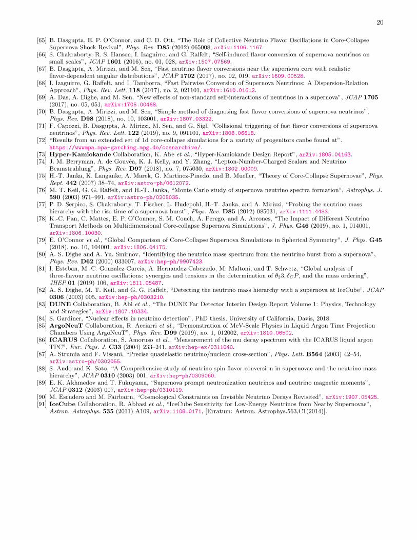
20

[65] B. Dasgupta, E. P. O’Connor, and C. D. Ott, “The Role of Collective Neutrino Flavor Oscillations in Core-CollapseSupernova Shock Revival”, Phys. Rev. D85 (2012) 065008, arXiv:1106.1167.

[66] S. Chakraborty, R. S. Hansen, I. Izaguirre, and G. Raffelt, “Self-induced flavor conversion of supernova neutrinos onsmall scales”, JCAP 1601 (2016), no. 01, 028, arXiv:1507.07569.

[67] B. Dasgupta, A. Mirizzi, and M. Sen, “Fast neutrino flavor conversions near the supernova core with realisticflavor-dependent angular distributions”, JCAP 1702 (2017), no. 02, 019, arXiv:1609.00528.

[68] I. Izaguirre, G. Raffelt, and I. Tamborra, “Fast Pairwise Conversion of Supernova Neutrinos: A Dispersion-RelationApproach”, Phys. Rev. Lett. 118 (2017), no. 2, 021101, arXiv:1610.01612.

[69] A. Das, A. Dighe, and M. Sen, “New effects of non-standard self-interactions of neutrinos in a supernova”, JCAP 1705(2017), no. 05, 051, arXiv:1705.00468.

[70] B. Dasgupta, A. Mirizzi, and M. Sen, “Simple method of diagnosing fast flavor conversions of supernova neutrinos”,Phys. Rev. D98 (2018), no. 10, 103001, arXiv:1807.03322.

[71] F. Capozzi, B. Dasgupta, A. Mirizzi, M. Sen, and G. Sigl, “Collisional triggering of fast flavor conversions of supernovaneutrinos”, Phys. Rev. Lett. 122 (2019), no. 9, 091101, arXiv:1808.06618.

[72] “Results from an extended set of 1d core-collapse simulations for a variety of progenitors canbe found at”.https://wwwmpa.mpa-garching.mpg.de/ccsnarchive/.

[73] Hyper-Kamiokande Collaboration, K. Abe et al., “Hyper-Kamiokande Design Report”, arXiv:1805.04163.[74] J. M. Berryman, A. de Gouvea, K. J. Kelly, and Y. Zhang, “Lepton-Number-Charged Scalars and Neutrino

Beamstrahlung”, Phys. Rev. D97 (2018), no. 7, 075030, arXiv:1802.00009.[75] H.-T. Janka, K. Langanke, A. Marek, G. Martinez-Pinedo, and B. Mueller, “Theory of Core-Collapse Supernovae”, Phys.

Rept. 442 (2007) 38–74, arXiv:astro-ph/0612072.[76] M. T. Keil, G. G. Raffelt, and H.-T. Janka, “Monte Carlo study of supernova neutrino spectra formation”, Astrophys. J.

590 (2003) 971–991, arXiv:astro-ph/0208035.[77] P. D. Serpico, S. Chakraborty, T. Fischer, L. Hudepohl, H.-T. Janka, and A. Mirizzi, “Probing the neutrino mass

hierarchy with the rise time of a supernova burst”, Phys. Rev. D85 (2012) 085031, arXiv:1111.4483.[78] K.-C. Pan, C. Mattes, E. P. O’Connor, S. M. Couch, A. Perego, and A. Arcones, “The Impact of Different Neutrino

Transport Methods on Multidimensional Core-collapse Supernova Simulations”, J. Phys. G46 (2019), no. 1, 014001,arXiv:1806.10030.

[79] E. O’Connor et al., “Global Comparison of Core-Collapse Supernova Simulations in Spherical Symmetry”, J. Phys. G45(2018), no. 10, 104001, arXiv:1806.04175.

[80] A. S. Dighe and A. Yu. Smirnov, “Identifying the neutrino mass spectrum from the neutrino burst from a supernova”,Phys. Rev. D62 (2000) 033007, arXiv:hep-ph/9907423.

[81] I. Esteban, M. C. Gonzalez-Garcia, A. Hernandez-Cabezudo, M. Maltoni, and T. Schwetz, “Global analysis ofthree-flavour neutrino oscillations: synergies and tensions in the determination of θ23, δCP , and the mass ordering”,JHEP 01 (2019) 106, arXiv:1811.05487.

[82] A. S. Dighe, M. T. Keil, and G. G. Raffelt, “Detecting the neutrino mass hierarchy with a supernova at IceCube”, JCAP0306 (2003) 005, arXiv:hep-ph/0303210.

[83] DUNE Collaboration, B. Abi et al., “The DUNE Far Detector Interim Design Report Volume 1: Physics, Technologyand Strategies”, arXiv:1807.10334.

[84] S. Gardiner, “Nuclear effects in neutrino detection”, PhD thesis, University of California, Davis, 2018.[85] ArgoNeuT Collaboration, R. Acciarri et al., “Demonstration of MeV-Scale Physics in Liquid Argon Time Projection

Chambers Using ArgoNeuT”, Phys. Rev. D99 (2019), no. 1, 012002, arXiv:1810.06502.[86] ICARUS Collaboration, S. Amoruso et al., “Measurement of the mu decay spectrum with the ICARUS liquid argon

TPC”, Eur. Phys. J. C33 (2004) 233–241, arXiv:hep-ex/0311040.[87] A. Strumia and F. Vissani, “Precise quasielastic neutrino/nucleon cross-section”, Phys. Lett. B564 (2003) 42–54,

arXiv:astro-ph/0302055.[88] S. Ando and K. Sato, “A Comprehensive study of neutrino spin flavor conversion in supernovae and the neutrino mass

hierarchy”, JCAP 0310 (2003) 001, arXiv:hep-ph/0309060.[89] E. K. Akhmedov and T. Fukuyama, “Supernova prompt neutronization neutrinos and neutrino magnetic moments”,

JCAP 0312 (2003) 007, arXiv:hep-ph/0310119.[90] M. Escudero and M. Fairbairn, “Cosmological Constraints on Invisible Neutrino Decays Revisited”, arXiv:1907.05425.[91] IceCube Collaboration, R. Abbasi et al., “IceCube Sensitivity for Low-Energy Neutrinos from Nearby Supernovae”,

Astron. Astrophys. 535 (2011) A109, arXiv:1108.0171, [Erratum: Astron. Astrophys.563,C1(2014)].