Embed Size (px)
Citation preview

On the Hierarchical Community Structure ofPractical SAT Formulas
Chunxiao Li1∗, Jonathan Chung1
∗, Soham Mukherjee1,2, Marc Vinyals3,
Noah Fleming4, Antonina Kolokolova5, Alice Mu1, and Vijay Ganesh1
1 University of Waterloo, Waterloo, Canada2 Perimeter Institute, Waterloo, Canada
3 Technion, Haifa, Israel4 University of Toronto, Toronto, Canada
5 Memorial University of Newfoundland, St. John’s, Canada
Abstract. Modern CDCL SAT solvers easily solve industrial instancescontaining tens of millions of variables and clauses, despite the theoret-ical intractability of the SAT problem. This gap between practice andtheory is a central problem in solver research. It is believed that SATsolvers exploit structure inherent in industrial instances, and hence therehave been numerous attempts over the last 25 years at characterizing thisstructure via parameters. These can be classified as rigorous, i.e., theyserve as a basis for complexity-theoretic upper bounds (e.g., backdoors),or correlative, i.e., they correlate well with solver run time and are ob-served in industrial instances (e.g., community structure). Unfortunately,no parameter proposed to date has been shown to be both strongly cor-relative and rigorous over a large fraction of industrial instances.Given the sheer difficulty of the problem, we aim for an intermediategoal of proposing a set of parameters that is strongly correlative and hasgood theoretical properties. Specifically, we propose parameters basedon a graph partitioning called Hierarchical Community Structure (HCS),which captures the recursive community structure of a graph of a Booleanformula. We show that HCS parameters are strongly correlative withsolver run time using an Empirical Hardness Model, and further build aclassifier based on HCS parameters that distinguishes between easy in-dustrial and hard random/crafted instances with very high accuracy. Wefurther strengthen our hypotheses via scaling studies. On the theoreticalside, we show that counterexamples which plagued community structuredo not apply to HCS, and that there is a subset of HCS parameters suchthat restricting them limits the size of embeddable expanders.
1 Introduction
Over the last two decades, Conflict-Driven Clause-Learning (CDCL) SAT solvershave had a dramatic impact on many sub-fields of software engineering [11], for-mal methods [14], security [18,47], and AI [9], thanks to their ability to solvelarge real-world instances with tens of millions of variables and clauses [40],
∗Joint first author

2 Li, Chung et al.
notwithstanding the fact that the Boolean satisfiability (SAT) problem is knownto be NP-complete and is believed to be intractable [17]. This apparent con-tradiction can be explained away by observing that the NP-completeness of theSAT problem is established in a worst-case setting, while the dramatic efficiencyof modern SAT solvers is witnessed over “practical” instances. However, despiteover two decades of effort, we still do not have an appropriate mathematicalcharacterization of practical instances (or a suitable subset thereof) and atten-dant complexity-theoretic upper and lower bounds. Hence, this gap betweentheory and practice is rightly considered as one of the central problems in solverresearch by theorists and practitioners alike.
The fundamental premise in this line of work is that SAT solvers are efficientbecause they somehow exploit the underlying structure in industrial Booleanformulas1, and further, that hard randomly-generated or crafted instances aredifficult because they do not possess such structure. Consequently, considerablework has been done in characterizing the structure of industrial instances viaparameters. The parameters discussed in literature so far can be broadly classi-fied into two categories, namely, correlative and rigorous2. The term correlativerefers to parameters that take a specific range of values in industrial instances (asopposed to random/crafted) and further have been shown to correlate well withsolver run time. This suggests that the structure captured by such parametersmight explain why solvers are efficient over industrial instances. An example ofsuch a parameter (resp. structure) is modularity (resp. community structure [4]).By contrast, the term rigorous refers to parameters that characterize classes offormulas that are fixed-parameter tractable (FPT), such as: backdoors [46,50],backbones [30], treewidth, and branchwidth [1,39], among many others [39]; orhave been used to prove complexity-theoretic bounds over randomly-generatedclasses of Boolean formulas such as clause-variable ratio (a.k.a., density) [16,41].
The eventual goal in this context is to discover a parameter or set of pa-rameters that is both strongly correlative and rigorous, such that it can thenbe used to establish parameterized complexity theoretic bounds on an appro-priate mathematical abstraction of CDCL SAT solvers, thus finally settling thisdecades-long open question. Unfortunately, the problem with all the previouslyproposed rigorous parameters is that either “good” ranges of values for theseparameters are not witnessed in industrial instances (e.g., such instances canhave both large and small backdoors) or they do not correlate well with solverrun time (e.g., many industrial instances have large treewidth and yet are easyto solve, and treewidth alone does not correlate well with solving time [29]).
Consequently, many attempts have been made at discovering correlative pa-rameters that could form the basis of rigorous analysis [4,23]. Unfortunately, allsuch correlative parameters either seem to be difficult to work with theoretically(e.g., fractal dimension [2]) or have obvious counterexamples, i.e., it is easy toshow the existence of formulas that simultaneously have “good” parameter val-
1The term industrial is loosely defined to encompass instances obtained from hard-ware and software testing, analysis, and verification applications.
2Using terminology by Stefan Szeider [44].

On the HCS of Practical SAT Formulas 3
ues and are provably hard-to-solve. For example, it was shown that industrialinstances have good community structure, i.e., high modularity [4], and thatthere is good-to-strong correlation between community structure and solver runtime [34]. However, Mull et al. [31] later exhibited a dense family of formulasthat have high modularity and require exponential-sized proofs to refute. Fi-nally, this line of research suffers from important methodological issues, that is,experimental methods and evidence provided for correlative parameters tend notto be consistent across different papers in the literature.
Hierarchical Community Structure of Boolean Formulas: Given thesheer difficulty of the problem, we aim for an intermediate goal of proposing aset of parameters that is strongly correlative and has good theoretical properties.Specifically, we propose a set of parameters based on a graph-theoretic struc-ture called Hierarchical Community Structure (HCS), inspired by a commonly-studied concept in the context of hierarchical networks [15,37], which satisfiesall the empirical tests hinted above and has better theoretical properties thanpreviously proposed correlative parameters. The intuition behind HCS is that itneatly captures the structure present in human-developed systems which tendto be modular and hierarchical [43], and we expect this structure to be inheritedby Boolean formulas modelling these systems.
Brief Overview of Results: Using a machine-learning (ML) classifier, we em-pirically demonstrate that the range of HCS-based parameter values taken byindustrial instances is distinct from the range of values taken by randomly-generated or crafted instances. The accuracy of our classifier is very high, andwe perform a variety of tests to ensure there is no over-fitting. We also showa good correlation between HCS-based parameter values and solver run time.From these two experiments, and in conjunction with theoretical analysis, wezero-in on three parameters as the most predictive, namely, leaf-community size,community degree, and the fraction of inter-community edges. To further under-stand their impact on solver run time, we perform several scaling studies whichfurther strengthen our case that HCS parameters hold promise in explaining thepower of CDCL SAT solvers over industrial instances.
Finally, we prove that HCS parameters have good theoretical properties.Specifically, we prove that linear expanders cannot be embedded in formulaswith “good” HCS parameters (i.e., small community leaf size, small communitydegree, and small number of inter-community edges). Further, we show that asthe range of parameter values improve, stronger varieties of expander graphs canbe ruled out. Strong expansion properties of the underlying graph of a formulaare one of the main tools used in proving proof complexity lower bounds.
Having said that, we also show that restricting certain subsets of these pa-rameters, while avoiding previously known counterexamples, can be shown toallow for formulas that require large resolution refutations. However, the con-struction of these counterexamples is non-trivial, and indeed significantly morecomplicated than the counterexamples which suffice for community structure[31].Nonetheless, we believe that hierarchy will eventually play an important role,

4 Li, Chung et al.
alongside other parameters, in settling the long-standing and difficult questionregarding the unreasonable performance of solvers over industrial instances.Research Methodology: We also codify into a research methodology a set ofempirical tests which we believe parameters must pass in order to be consideredfor further theoretical analysis. While other researchers have considered one ormore of these tests, we bring them together into a coherent and sound researchmethodology that can be used for future research in formula parameterization.These empirical tests include the following: first, there must exist strong sta-tistical evidence (in the form of well-understood correlation measures and MLpredictors) that witnesses the presence of the proposed structure (in terms ofa range of proposed parameter values) in industrial instances and its absencefrom random or crafted ones; second, strong statistical evidence for correlationbetween sharply-defined good (resp. bad) values of parameters and low (resp.high) solver running time; third, independent parameter scaling that enablesthe isolation of the effects of each parameter. We believe that the combinationof these requirements provides a strong basis for a correlative parameter to beconsidered worthy of further analysis.
Detailed List of Contributions3:
1. Empirical Result 1 (HCS and Industrial Instances): As stated above,we propose a set of parameters based on HCS of the variable-incidence graph(VIG) of Boolean formulas, and show that they are very effective in distin-guishing industrial instances from random/crafted ones. In particular, webuild a classifier that classifies SAT instances into the problem categoriesthey belong to (e.g., industrial and randomly-generated). We show that ourHCS parameters are robust in classifying SAT formulas into problem cate-gories. The classification accuracy is approximately 99% and we perform avariety of tests to ensure there is no overfitting (See Section 5.2).
2. Empirical Result 2 (Correlation between HCS and Solver RunTime): We build an empirical hardness model based on our HCS parametersto predict the solver run time for a given problem instance. Our model, basedon regression, performs well, achieving an adjusted R2 score of 0.85, muchstronger than previous such results (see Section 5.3).
3. Empirical Result 3 (Scaling Experiments of HCS Instances): Weempirically show, via scaling experiments, that HCS parameters such asdepth and leaf-community size positively correlate with solving time. Finally,we empirically show that formulas whose HCS decompositions fall in a goodrange of parameter values are easier to solve than instances with a bad rangeof HCS parameter values (See Section 5.5).
4. Theoretical Results: We theoretically justify our choice of HCS by show-ing that it behaves better than other parameters. More concretely, we showthe advantages of hierarchical over flat community structure by identifyingHCS parameters which let us avoid hard formulas that can be used as coun-terexamples to community structure [31], and by showing graphs where HCS
3Instance generator, data, and full paper can be found here: https://
satcomplexity.github.io/hcs/

On the HCS of Practical SAT Formulas 5
can find the proper communities where flat modularity cannot. We also showthat there is a subset of HCS parameters (leaf-community size, communitydegree, and inter-community edges) such that restricting them limits the sizeof embeddable expanders.
5. Instance Generator: Finally, we provide an HCS-based instance gener-ator which takes input values of our proposed parameters and outputs arecursively generated formula that satisfies those values. This generator canbe used to generate “easy” and “hard” formulas with different hierarchicalstructures.
2 Preliminaries
Variable Incidence Graph (VIG): Researchers have proposed a variety ofgraphs to study graph-theoretic properties of Boolean formulas. In this work,we focus on the Variable Incidence Graph (VIG) model of Boolean formulas,primarily due to the relative ease of computing community structure over VIGscompared to other graph representations. The VIG for a formula F over variablesx1, . . . , xn has n vertices, one for each variable. There is an edge between verticesxi and xj if both xi and xj occur in some clause Ck in F . One drawback of VIGsis that a clause of width w corresponds to a clique of size w in the VIG. Therefore,large width clauses (of size nε) can significantly distort the structure of a VIG,and formulas with such large width clauses should have their width reduced (viastandard techniques) before using a VIG.Community Structure and Modularity: Intuitively, a set of variables (ver-tices in the VIG) of a formula forms a community if these variables are moredensely connected to each other than to variables outside of the set. An (optimal)community structure of a graph is a partition P = V1, . . . , Vk of its verticesinto communities that optimizes some measure capturing this intuition, for in-stance modularity [32], which is the one we use in this paper. Let G = (V,E)be a graph with adjacency matrix A and for each vertex v ∈ V denote by d(v)its degree. Let δP : V × V → 0, 1 be the community indicator function of apartition, i.e. δP (u, v) = 1 iff vertices u and v belong to the same community inP . The modularity of the partition P is
Q(P ) :=1
2|E|∑u,v∈V
[Au,v −
d(u)d(v)
2|E|
]δP (u, v) (1)
Note that Q(P ) ranges from −0.5 to 1, with values close to 1 indicating goodcommunity structure. We define the modularity Q(G) of a graph G as the maxi-mum modularity over all possible partitions, with corresponding partition P(G).Other measures may produce radically different partitions.Expansion of a Graph: Expansion is a measure of graph connectivity [25].Out of several equivalent such measures, the most convenient for HCS is theedge expansion: given a subset of vertices S ⊆ V , its edge expansion is h(S) =|E(S, V \S)|/|S|, and the edge expansion of a graph is h(G) = min1≤|S|≤n/2 h(S).

6 Li, Chung et al.
A graph family Gn is an expander if h(Gn) is bounded away from zero. Reso-lution lower bounds (of both random and crafted formulas) often rely on strongexpansion properties of the graph [6].
3 Research Methodology
As stated above, the eventual goal of the research presented here is to discovera structure and an associated parameterization that is highly correlative withsolver run time, is witnessed in industrial instances, and is rigorous, i.e., formsthe basis for an upper bound on the parameterized complexity [39] of the CDCLalgorithm. Considerable work has already been done in attempting to identifyexactly such a set of parameters [34]. However, we observed that there is a widediversity of research methodologies adopted by researchers in the past. We bringtogether the best lessons learned into what we believe to be a sound, coherent,and comprehensive research methodology explained below. We argue that everyset of parameters must meet the following empirical requirements in order to beconsidered correlative and possibly rigorous:
1. Structure of Industrial vs. Random/Crafted Instances: A prerequi-site for a structure to be considered correlative is that industrial instancesmust exhibit a certain range of values for the associated parameters, whilerandom and crafted instances must have a different distinct range of param-eter values. An example of such a structure is the community structure ofthe VIG of Boolean formulas, as parameterized by modularity. Multiple ex-periments have shown that industrial instances have high modularity (closeto 1), while random instances tend to have low modularity (close to 0) [34].This could be demonstrated via a correlation experiment or by using a ma-chine learning classifier that takes parameter values as input features andclassifies instances as industrial, random, crafted etc. with high accuracy.
2. Correlation between Structure and Solver Run Time: Another re-quirement for a structure to be considered correlative is demonstrating thatthere is indeed correlation between parameters of a structure and solver runtime. Once again, community structure (and the associated modularity pa-rameter) forms a good example of a structure that passes this essential test.It has been shown that the modularity of the community structure of indus-trial instances (resp. random instances) correlates well with low (resp. high)solver run time. One may use either correlation methods or suitable machinelearning predictors (e.g., random forest) as evidence here.
3. Scaling Studies: To further strengthen the experimental evidence, we re-quire that the chosen structure and its associated parameters must pass anappropriately designed scaling study. The idea here is to vary one parametervalue while keeping as much of the rest of the formula structure constant aspossible, and see its effect on solver run time. An example of such a parame-ter is mergeability. In their work, Zulkoski et al. [49] showed that increasingthe mergeability metric has a significant effect on solver run time.

On the HCS of Practical SAT Formulas 7
Limitations of Empirical Conclusions: As the reader is well aware, any at-tempt at empirically discovering a suitable structure (and associated parameteri-zation) of Boolean formulas and experimentally explaining the power of solvers isfraught with peril, since all such experiments involve pragmatic design decisions(e.g., which solver was used, choice of benchmarks, etc.) and hence may lead tocontingent or non-generalizable conclusions. For example, one can never quiteeliminate a parameter from further theoretical analysis based on empirical testsalone, for the parameter may fail an empirical test on account of benchmarksconsidered or other contingencies. Another well-understood issue with conclu-sions based on empirical analysis alone is that they by themselves cannot implyprovable statements about asymptotic behavior of algorithms. However, one canuse empirical analysis to check or expose gaps between the behavior of an algo-rithm and the tightness of asymptotic statements (e.g., the gap between efficienttypical-case behavior vs. loose worst-case statements). Having said all this, webelieve that the above methodology is a bare minimum that a set of parame-ters must pass before being considered worthy of further theoretical analysis.In Section 5.1, we go into further detail about how we protect against certaincontingent experimental conclusions.Limits of Theoretical Analysis: Another important aspect to bear in mindis that it is unlikely any small set of parameters can cleanly separate all easyinstances from hard ones. At best, our expectation is that we can characterize alarge subset of easy real-world instances via the parameters presented here, andthus take a step towards settling the central question of solver research.
4 Hierarchical Community Structure
Given that many human-developed systems are modular and hierarchical [43],it is natural to hypothesize that these properties are transferred over to Booleanformulas that capture the behaviour of such systems. We additionally hypothe-size that purely randomly-generated or crafted formulas do not have these prop-erties of hierarchy and modularity, and that this difference partly explains whysolvers are efficient for the former and not for the latter class of instances. Weformalize this intuition via a graph-theoretic concept called Hierarchical Commu-nity Structure (HCS), where communities can be recursively decomposed intosmaller sub-communities. Although the notion of HCS has been widely stud-ied [15,37], it has not been considered in the context of Boolean formulas before.
Hierarchical Community Structure Definition: A hierarchical decomposi-tion of a graph G is a recursive partitioning of G into subgraphs, represented as atree T . Each node v in the tree T is labelled with a subgraph of G, with the rootlabelled with G itself. The children of a node corresponding to a (sub)graph Hare labelled with a partitioning of H into subgraphs H1, . . . ,Hk; see Figure 1.There are many ways to build such hierarchical decompositions. The methodthat we choose constructs the tree by recursively maximizing the modularity, asin the hierarchical multiresolution method [24]. We call this the HCS decompo-sition of a graph G: for a node v in the tree T corresponding to a subgraph H

8 Li, Chung et al.
G11
G12 G22
G21
G1 G2
G11 G12 G22G21
G1 G2
Fig. 1. A hierarchical decomposition (right) constructed by recursively maxi-mizing the modularity of the graph (left).
of G, we construct |P(H)| children, one for each of the subgraphs induced bythe modularity-maximizing partition P(H), unless |P(H)| = 1, in which case vbecomes a leaf of the tree. In the case of HCS decompositions, we refer to thesubgraphs labelling the nodes in the tree as communities of G.
We are interested in comparing the hierarchical community structures ofBoolean formulas in conjunctive normal form, represented by their VIGs. Forthis comparison, we use the following parameters:
– The community degree of a community in a HCS decomposition is the num-ber of children of its corresponding node.
– A leaf-community is one with degree 0.
– The size of a community is its number of vertices.
– The depth or level of a community is its distance from the root.
– For a given partition of a graph H, the inter-community edges are EIC (H) =⋃i,j E(Hi, Hj), the edges between all pairs of subgraphs, and their endpoints
VIC (H) =⋃EIC are the inter-community vertices. Note that 2|EIC (H)|/|H|
is an upper bound for the edge expansion of H.
Note that these parameters are not independent. For example, changes in thenumber of inter-community vertices or inter-community edges will affect modu-larity. Since our hierarchical decomposition is constructed using modularity, thiscould affect the entire decomposition and hence the other parameters. In fact, inour experiments we use 49 different parameters of the HCS structure and thenidentify the most predictive ones among them. It turns out that leaf-communitysize (i.e., number of nodes in leaves of the HCS of a VIG), community degree,and inter-community edges are among the most predictive (See Section 5). Ingeneral, formulas with small community size, small community degree and fewinter-community edges are easier to solve (See Section 5.6).

On the HCS of Practical SAT Formulas 9
Table 1. Summary of benchmark instances
Class Name #SAT #UNSAT #UNKNOWN
agile 372 475 8crafted 300 99 617crypto 1052 355 3496random 276 224 661verification 197 2345 392
5 Empirical Results
5.1 Experimental Design
Choice of SAT Solver: We pre-process all formulas using standard tech-niques [28] and use MapleSAT as our CDCL solver of choice since it is a leadingand representative solver [28].Choice of Benchmark Suite: In our experiments, we use a set of 10 869instances from five different instance classes, which we believe is sufficientlylarge and diverse to draw sound empirical conclusions. We do not explicitlybalance the ratio of satisfiable instances in our benchmark selection because weexpect our methods to be sufficiently robust as long as the benchmark containsa sufficient number of SAT and UNSAT instances.
In order to get interesting instances for modern solvers, we consider formu-las which were previously used in the SAT competition from 2016 to 2018 [40].Specifically, we take instances from five major tracks of the competition: Agile,Verification, Crypto, Crafted, and Random. We also generate additionalinstances for some classes: for verification, we scale the number of unrolls whenencoding finite state machines for bounded model checking; for crypto, we encodeSHA-1 and SHA-256 preimage problems; for crafted, we generate combinatorialproblems using cnfgen [27]; and for random, we generate k-CNFs at the corre-sponding threshold CVRs for k ∈ 3, 5, 7, again using cnfgen. A summary ofthe instances is presented in Table 1.Computational Resources: For computing satisfiability and running time,we use SHARCNET’s Intel E5-2683 v4 (Broadwell) 2.1 GHz processors [42],limiting the computation time to 5000 seconds4. For parameter computation,we still use SHARCNET, but we do not limit the type of processor becausestructural parameter values are independent of processing power.Choice of Community Detection Algorithm: In our experiments, we usethe Louvain method [8] to detect communities, taking the top-level partition asour communities. The Louvain method is typically more efficient and produceshigher-modularity partitions than other known algorithms.Parameters: We consider a small number of base parameters, in addition toHCS-based ones, to measure different structural properties of input VIGs. The
4This value is the time limit used by the SAT competition.

10 Li, Chung et al.
base parameters are the number of variables, clauses, and binary clauses; theaverage and variance in the number of occurrences of each variable; the num-ber of inter-community variables and inter-community edges; the numbers, sizes,degrees, and depths of the communities; modularity; and mergeability (see sup-plementary material5 for a comprehensive list of parameter combinations).
5.2 HCS-based Category Classification of Boolean Formulas
It is conjectured that SAT solvers are efficient because they somehow exploitthe underlying structure in industrial formulas. One may then ask the questionwhether our set of HCS parameters is able to capture the underlying structurethat differentiates industrial instances from the rest, which naturally lends itselfto a classification problem. Therefore, we build a multi-class Random Forestclassifier to classify a given SAT instance into one of five categories: verification,agile, random, crafted, or crypto. Random Forests [10] are known for their abilityto learn complex, highly non-linear relationships while having simple structure,and hence are easier to interpret than other models (e.g., deep neural networks).
We use an off-the-shelf implementation of a Random Forest classifier im-plemented as sklearn.ensemble.RandomForestClassifier in scikit-learn [35].We train our classifier using 800 randomly sampled instances of each category ona set of 49 features to predict the class of the problem instance. We find that ourclassifier performs extremely well, giving an average accuracy score of 0.99 overmultiple cross-validation datasets. Our accuracy does not depend on our choiceof classifier. We find similar accuracy scores when we use C-Support Vector clas-sification [36]. Further, we determine the five most important features used byour classifier. Since some of our features are highly correlated, we first performa hierarchical clustering on the feature set based on Spearman rank-order cor-relations, choose a single feature from each cluster, and then use permutationimportance [10] to compute feature importance. We present results in Table 2.
The robustness of our classifier indicates that HCS parameters are represen-tative of the underlying structure of Boolean formulas from different categories.In the following section, we discuss an empirical hardness model for predictingthe run time of the solver using the same set of features we used to classifyinstances into categories.
5.3 HCS-based Empirical Hardness Model
We use our HCS parameters to build an empirical hardness model (EHM) topredict the run time of a given instance for a particular solver (MapleSAT). Sincethe solving time is a continuous variable, we consider a regression model builtusing Random Forests. We use sklearn.ensemble.RandomForestRegressor,an implementation available in scikit-learn [35]. Before training our regressionmodel, we remove instances which timed-out at 5 000 seconds as well as those
5The supplemental material is available here as part of the full version of the paper:https://satcomplexity.github.io/hcs/

On the HCS of Practical SAT Formulas 11
Table 2. Results for classification and regression experiments. For regression wereport adjusted R2 values, whereas for classification, we report the mean of thebalanced accuracy score, over 5 cross-validation datasets.
Category Runtime
Score 0.996 ± 0.001 0.848 ± 0.009
Top 5 features
rootMergeability
maxInterEdges/CommunitySize
cvr
leafCommunitySize
lvl2InterEdges/lvl2InterVars
rootInterEdges
lvl2Mergeability
cvr
leafCommunitySize
lvl3Modularity
instances that were solved almost immediately (i.e., zero seconds) to avoid issueswith artificial cut-off boundaries. We then train our Random Forest model topredict the logarithm of the solving time using the remaining 1 880 instances,equally distributed between different categories.
We observe that our regression model performs quite well, with an adjustedR2 score of 0.84, which implies that in the training set, almost 84% of thevariability of the dependent variable (i.e., in our case, the logarithm of the solvingtime) is accounted for, and the remaining 16% is still unaccounted for by ourchoice of parameters. Similar to category classification, we also look for the topfive predictive features used by our Random Forest regression model using thesame process. We list the parameters in Table 2.
As a check, we train our EHM on each category of instances separately. Wefind that the performance of our EHM varies with instance category. Concretely,agile outperforms all other categories with an adjusted R2 value of 0.94, fol-lowed by random, crafted and verification instances with scores of 0.81, 0.85and 0.74 respectively. The worst performance is shown by the instances incrypto, with a score of 0.48. This suggests that our choice HCS parametersare more effective in capturing the hardness or easiness of formulas from indus-trial/agile/random/crafted, but not crypto. The crypto class is an outlier and itis not clear from our experiments (nor any previous experiments we are awareof) why crypto instances are hard for CDCL solvers.Top-5 Parameters: The top features identified in our classification and regres-sion experiments fall into five distinct classes of parameters: mergeability-based,modularity-based, inter-community edge based, CVR, and leaf-community size.
5.4 Scaling Studies of Industrial and Random Instances
In this experiment, we scaled the values of the top-5 formula parameters, iden-tified by the classification and regression experiments given above, to get a fine-grained picture of the impact of these parameters on solver run time. The param-eters CVR, mergeability and modularity have been studied by previous work.

12 Li, Chung et al.
log(# of variables)
root
inte
rcom
mun
ity e
dges
100
1000
10000
100000
100 1000 10000 100000
verification
(a) Verification
log(# of variables)
root
inte
rcom
mun
ity e
dges
1000
10000
100000
1000000
1000
2000
4000
6000
8000
1000
020
000
random
(b) Random
Fig. 2. Number of root-level inter-community edges vs. number of variables, byinstance class. All values are plotted on a logarithmic scale.
CVR is perhaps the most studied parameter among the three [12]. Zulkoski etal. [49] showed that mergeability, along with combinations of other parameters,correlates well with solver run time; Ansotegui et al. [4] showed that industrialinstances have good modularity compared to random instances; and Newshamet al. [34] showed that modularity has good-to-strong correlation with solver runtime. We more closely examine the remaining parameters: leaf-community sizeand inter-community edge based parameters.
We next show that the range of values rootInterEdges takes for industrialinstances is different from random instances, and we discuss the effect of scalingleaf-community size in Section 5.5. As we can see in Figure 2 (note that there arethree separate data series in the random subplot, corresponding to random 3-,5-, and 7-CNFs when ordered by growth rate), the number of inter-communityedges at the root level grows proportionally to the number of variables of theformula, while the proportionality constant for random instances is at least anorder of magnitude larger (two and three orders respectively for 5- and 7-CNFs).
5.5 Scaling via Instance Generator
In the experiments described here, we use an HCS instance generator to scale ourHCS parameters individually while holding other parameters constant. We gener-ate many instances with different HCS parameter values by specifying parametervalues of CVR, power law parameter, hierarchical degree, depth, leaf-communitysize, inter-community edge density, inter-community variable density, and clausewidth. We note that in our generator, modularity is specified implicitly throughthe above parameters, and we do not control for mergeability at all. We refer thereader to the works by Zulkoski et al. [49] and Giraldez-Cru [22] for literatureon the empirical behaviours of mergeability and power law respectively.
Our HCS instance generator is not intended to be perfectly representativeof real-world instances. In fact, there are multiple properties of our generatedinstances which are not reflective of industrial instances. For example, our gen-erator assumes that all leaf-communities have the same size and depth, which

On the HCS of Practical SAT Formulas 13
is demonstrably untrue of industrial instances. In some cases, the communitiesproduced by our generator might not be the same as the communities whichwould be detected using the Louvain method to perform a hierarchical commu-nity decomposition. For example, it might be possible to further decompose thegenerated “leaf-communities” into smaller communities. The generator is onlyintended to demonstrate the effect of varying our HCS parameters.Results: We show that when fixing every other HCS parameters, increasingany of leaf-community size, depth and community degree increases the overallhardness of the generated formula. This suggests that leaf-community size, depthand community degree are important HCS parameters to consider further.
5.6 Analysis of Empirical Results
The goal of our experimental work was to first ascertain whether HCS structureis witnessed in industrial instances, whether the parameter range is differentbetween industrial and random/crafted, and finally whether there is any corre-lation with solver run time. On all three counts, the answer is a strong yes. Inmore detail, after identifying the top-5 parameters (namely, mergeability-basedparameters, modularily-based parameters, CVR, leaf-community size, and inter-community edges) and based on the classification results, we can safely say thatthe HCS structure of industrial instances is empirically very different from thatof random/crafted. In particular, industrial instances typically have small leaf-community size, high modularity, and low inter-community edges, while ran-dom/crafted have larger leaf-community size, low modularity, and a very highnumber of inter-community edges. Further, the correlation with solver run timeis strong — much stronger than previously proposed parameters.
6 Theoretical Results
We present the following theoretical results that further strengthen the idea thatHCS-based parameters (especially ones identified above in analysis of experimen-tal results) may play a role in the final analysis of understanding of why SATsolvers are efficient over industrial instances. Based on our experimental work,we narrow down the most predictive HCS parameters to be leaf-community size,community degree, and inter-community edges. All of these parameters playa role in the theorems below. For a formula to have “good” HCS, we restrictthe parameter value range as follows: the graph must exhibit small O(log n)leaf-community size, constant community degree, and have a small number ofinter-community edges in each community.
Ideally, we would like to be able to theoretically establish a parameterizedupper bound via HCS parameters. Unfortunately, our current state of under-standing does not yet allow for that. A step towards such a result would beto show that formulas with good HCS (and associated parameter value ranges)form a family of instances such that typical methods of proving resolution lowerbounds, such as those exploiting expansion properties [6], do not apply to them.

14 Li, Chung et al.
More precisely, we would like to show that formulas with good HCS do not haveVIGs which are expanders or have large expanders embedded in them, since mostresolution lower bounds rely on expansion properties. In particular, for formulaswith low width, edge expansion is closely related to boundary expansion, theparameter of choice for proving resolution lower bounds. With this in mind, westate several positive and negative results.
First, we make the observation that we restrict leaf communities of the HCSof a graph to have size O(log n) to avoid counterexamples where large hardformulas are emdedded within them [31]. Indeed, practical instances having smallleaf communities is supported by our experimental results. Further, we observethat if the number of inter-community edges at the top level of the decompositiongrows sub-linearly with n and at least two sub-communities contain a constantfraction of vertices, then this graph family is not an expander.
Unfortunately, we can also show that graphs with good HCS can simultane-ously have sub-graphs that are large expanders, with the worst case being verysparse expanders, capable of “hiding” in the hierarchical decomposition by con-tributing relatively few edges to any cut. To avoid that, we require an explicitbound on the number of inter-community edges, in addition to small communitydegree and small leaf-community size. This lets us prove the following statement.
Theorem 1. Let G = Gn be a family of graphs. Let f(n) ∈ ω(poly(log n)),f(n) ∈ O(n). Assume that G has HCS with the number of inter-community edgeso(f(n)) for every community C of size at least Ω(f(n)) and depth is bounded byO(log n). Then G does not contain an expander of size f(n) as a subgraph.
Note that our experiments show that the leaf size and depth in industrialinstances are bounded by O(log n) and the number of inter-community edgesgrows slowly. From this and the theorem above, we can show that graphs withvery good HCS do not contain linear-sized expanders.
Hierarchical vs. Flat Modularity: It is well-known that modularity suffersfrom a resolution limit and cannot detect communities smaller than a certainthreshold [19], and it is also known that HCS can avoid this problem in someinstances [8]. We provide an asymptotic, rigorous statement of this observation.
Theorem 2. There exists a graph G whose natural communities are of sizelog(n) and correspond to the (leaf) HCS communities, while the partition maxi-
mizing modularity consists of communities of size Θ(√
n/ log3 n).
7 Related Work
7.1 Correlative Parameters and Empirical Models
Community Structure: Using modularity to measure community structureallows one to distinguish industrial instances from randomly-generated ones [4].Unfortunately, it has been shown that expanders can be embedded within formu-las with high modularity [31], i.e., there exist formulas that have good community
On the HCS of Practical SAT Formulas 15
structure and yet are hard for solvers. Although we identify this parameter ascorrelative, FPT results exist for a related concept, hitting community structureand h-modularity [21]. However, there is no evidence that hitting communitystructure is witnessed in industrial instances.
Heterogeneity: Unlike uniformly-random formulas, the variable degrees in in-dustrial formulas follow a powerlaw distribution [3]. However, degree heterogene-ity alone fails to explain the hardness of SAT instances. Some heterogeneousrandom k-SAT instances were shown to have superpolynomial resolution size[7], making them intractable for current solvers.
SATzilla: SATzilla uses 138 disparate parameters [48], some of which are probesaimed at capturing a SAT solver’s state at runtime, to predict solver runningtime. Unfortunately, there is no evidence that these parameters are amenable totheoretical analysis.
7.2 Rigorous Parameters
Clause-Variable Ratio (CVR): Cheeseman et al. [12] observed the satisfia-bility threshold behavior for random k-SAT formulas, where they show formulasare harder when their CVR are closer to the satisfiability threshold. Outside ofextreme cases, CVR alone seems to be insufficient to explain hardness (or easi-ness) of instances, as it is possible to generate both easy and hard formulas withthe same CVR [20]. Satisfiability thresholds are poorly defined for industrial in-stances, and Coarfa et al. [16] demonstrated the existence of instances for whichthe satisfiability threshold is not equal to the hardness threshold.
Treewidth: Although there are polynomial-time non-CDCL algorithms for SATinstances with bounded treewidth [1], treewidth by itself does not appear to bea predictive parameter of CDCL solver runtime. For example, Mateescu [29]showed that some easy instances have large treewidth, and later it was shownthat treewidth alone does not seem to correlate well with solving time [49].
Backdoors: In theory, the existence of small backdoors [46,38] should allowCDCL solvers to solve instances quickly, but empirically backdoors have beenshown not to strongly correlate with CDCL solver run time [26]. To the best ofour knowledge, the literature does not contain any strong empirical support forbackdoors alone as a predictive parameter.
8 Conclusions and Future Work
In this paper, we propose hierarchical community structure as a correlative pa-rameter for explaining the power of CDCL SAT solvers over industrial instances.Empirically, HCS parameters are much more predictive than previously proposedcorrelative parameters in terms of classifying instances into random/craftedvs. industrial, and in terms of predicting solver run time. We further identifythe following core HCS parameters that are the most predictive, namely, leaf-community size, modularity, and inter-community edges. Indeed, these same

16 Li, Chung et al.
parameters also play a role in our subsequent theoretical analysis. On the theo-retical side, we show that counterexamples which plagued flat community struc-ture do not apply to HCS, and that there is a subset of HCS parameters suchthat restricting them limits the size of embeddable expanders. In the final anal-ysis, we believe that HCS, along with other parameters such as mergeability orheterogeneity, will play a role in finally settling the question of why solvers areefficient over industrial instances.
References
1. Alekhnovich, M., Razborov, A.: Satisfiability, branch-width and Tseitintautologies. computational complexity 20(4), 649–678 (Dec 2011).https://doi.org/10.1007/s00037-011-0033-1
2. Ansotegui, C., Bonet, M.L., Giraldez-Cru, J., Levy, J.: The fractal dimension ofSAT formulas. In: Proceedings of the 7th International Joint Conference on Auto-mated Reasoning - IJCAR 2014. pp. 107–121 (2014). https://doi.org/10.1007/978-3-319-08587-6 8
3. Ansotegui, C., Bonet, M.L., Levy, J.: Towards industrial-like random SAT in-stances. In: IJCAI 2009, Proceedings of the 21st International Joint Conferenceon Artificial Intelligence. pp. 387–392 (2009)
4. Ansotegui, C., Giraldez-Cru, J., Levy, J.: The community structure of SATformulas. In: Proceedings of the 15th International Conference on Theoryand Applications of Satisfiability Testing - SAT 2012. pp. 410–423 (2012).https://doi.org/10.1007/978-3-642-31612-8 31
5. Beame, P., Pitassi, T.: Simplified and improved resolution lower bounds. In: 37thAnnual Symposium on Foundations of Computer Science, FOCS ’96, Burlington,Vermont, USA, 14-16 October, 1996. pp. 274–282. IEEE Computer Society (1996).https://doi.org/10.1109/SFCS.1996.548486
6. Ben-Sasson, E., Wigderson, A.: Short proofs are narrow—resolution made simple.Journal of the ACM (JACM) 48(2), 149–169 (2001)
7. Blasius, T., Friedrich, T., Gobel, A., Levy, J., Rothenberger, R.: The impact ofheterogeneity and geometry on the proof complexity of random satisfiability. In:Proceedings of the 2021 ACM-SIAM Symposium on Discrete Algorithms, SODA2021. pp. 42–53 (2021). https://doi.org/10.1137/1.9781611976465.4
8. Blondel, V., Guillaume, J.L., Lambiotte, R., Lefebvre, E.: Fast unfolding of commu-nities in large networks. Journal of Statistical Mechanics Theory and Experiment2008 (Apr 2008). https://doi.org/10.1088/1742-5468/2008/10/P10008
9. Blum, A.L., Furst, M.L.: Fast planning through planning graph analysis. Artificialintelligence 90(1-2), 281–300 (1997)
10. Breiman, L.: Random forests. Mach. Learn. 45(1), 5–32 (Oct 2001).https://doi.org/10.1023/A:1010933404324, https://doi.org/10.1023/A:
1010933404324
11. Cadar, C., Ganesh, V., Pawlowski, P.M., Dill, D.L., Engler, D.R.: EXE: Automat-ically generating inputs of death. ACM Transactions on Information and SystemSecurity (TISSEC) 12(2), 1–38 (2008)
12. Cheeseman, P., Kanefsky, B., Taylor, W.M.: Where the really hard problems are.In: Proceedings of the 12th International Joint Conference on Artificial Intelligence.pp. 331–337. IJCAI’91 (1991)

On the HCS of Practical SAT Formulas 17
13. Chvatal, V., Szemeredi, E.: Many hard examples for resolution. J. ACM 35(4),759–768 (1988). https://doi.org/10.1145/48014.48016
14. Clarke Jr, E.M., Grumberg, O., Kroening, D., Peled, D., Veith, H.: Model checking.MIT press (2018)
15. Clauset, A., Moore, C., Newman, M.E.J.: Hierarchical structure and the pre-diction of missing links in networks. Nature 453(7191), 98–101 (May 2008).https://doi.org/10.1038/nature06830
16. Coarfa, C., Demopoulos, D.D., San Miguel Aguirre, A., Subramanian, D., Vardi,M.Y.: Random 3-SAT: The plot thickens. Constraints 8(3), 243–261 (Jul 2003).https://doi.org/10.1023/A:1025671026963
17. Cook, S.A.: The complexity of theorem-proving procedures. In: Proceedings ofthe 3rd Annual ACM Symposium on Theory of Computing. pp. 151–158 (1971).https://doi.org/10.1145/800157.805047
18. Dolby, J., Vaziri, M., Tip, F.: Finding bugs efficiently with a SAT solver. In: Pro-ceedings of the 6th joint meeting of the European Software Engineering Conferenceand the ACM SIGSOFT International Symposium on Foundations of Software En-gineering. pp. 195–204 (2007). https://doi.org/10.1145/1287624.1287653
19. Fortunato, S., Barthelemy, M.: Resolution limit in community detection.Proceedings of the National Academy of Sciences 104(1), 36–41 (2007).https://doi.org/10.1073/pnas.0605965104
20. Friedrich, T., Krohmer, A., Rothenberger, R., Sutton, A.M.: Phase transitions forscale-free SAT formulas. In: Proceedings of the Thirty-First AAAI Conference onArtificial Intelligence. p. 3893–3899. AAAI’17, AAAI Press (2017)
21. Ganian, R., Szeider, S.: Community structure inspired algorithms for SATand #SAT. In: Proceedings of the 18th International Conference on Theoryand Applications of Satisfiability Testing - SAT 2015. pp. 223–237 (2015).https://doi.org/10.1007/978-3-319-24318-4 17
22. Giraldez-Cru, J.: Beyond the Structure of SAT Formulas. Ph.D. thesis, UniversitatAutonoma de Barcelona (2016)
23. Giraldez-Cru, J., Levy, J.: A modularity-based random SAT instances generator.In: Proceedings of the Twenty-Fourth International Joint Conference on ArtificialIntelligence, IJCAI 2015. pp. 1952–1958 (2015), http://ijcai.org/Abstract/15/277
24. Granell, C., Gomez, S., Arenas, A.: Hierarchical multiresolution method to over-come the resolution limit in complex networks. International journal of bifurcationand chaos 22(07), 1250171 (2012)
25. Hoory, S., Linial, N., Wigderson, A.: Expander graphs and their applications. Bul-letin of the American Mathematical Society 43(4), 439–561 (2006)
26. Kilby, P., Slaney, J., Thiebaux, S., Walsh, T.: Backbones and backdoors in satisfi-ability. In: Proceedings of the National Conference on Artificial Intelligence. vol. 3,pp. 1368–1373 (Jan 2005)
27. Lauria, M., Elffers, J., Nordstrom, J., Vinyals, M.: CNFgen: A generator of craftedbenchmarks. In: Proceedings of the 20th International Conference on Theoryand Applications of Satisfiability Testing (SAT ’17). pp. 464–473 (Aug 2017).https://doi.org/10.1007/978-3-319-94144-8 18
28. Liang, J.H., Ganesh, V., Poupart, P., Czarnecki, K.: Learning rate based branchingheuristic for SAT solvers. In: Proceedings of the 19th International Conference onTheory and Applications of Satisfiability Testing - SAT 2016. pp. 123–140 (2016).https://doi.org/10.1007/978-3-319-40970-2 9

18 Li, Chung et al.
29. Mateescu, R.: Treewidth in industrial sat benchmarks. Tech. Rep. MSR-TR-2011-22, Microsoft (Feb 2011), https://www.microsoft.com/en-us/research/
publication/treewidth-in-industrial-sat-benchmarks/
30. Monasson, R., Zecchina, R., Kirkpatrick, S., Selman, B., Troyansky, L.: Deter-mining computational complexity from characteristic ‘phase transitions’. Nature400(6740), 133–137 (1999)
31. Mull, N., Fremont, D.J., Seshia, S.A.: On the hardness of SAT with commu-nity structure. In: Proceedings of the 19th International Conference on The-ory and Applications of Satisfiability Testing (SAT). pp. 141–159 (Jul 2016).https://doi.org/10.1007/978-3-319-40970-2 10
32. Newman, M.E.J., Girvan, M.: Finding and evaluating commu-nity structure in networks. Physical Review E 69(2) (Feb 2004).https://doi.org/10.1103/physreve.69.026113
33. Newman, M.E.: Modularity and community structure in networks. Proceedings ofthe national academy of sciences 103(23), 8577–8582 (2006)
34. Newsham, Z., Ganesh, V., Fischmeister, S., Audemard, G., Simon, L.: Impact ofcommunity structure on SAT solver performance. In: Theory and Applications ofSatisfiability Testing - SAT 2014 - 17th International Conference, Held as Partof the Vienna Summer of Logic, VSL 2014, Vienna, Austria, July 14-17, 2014.Proceedings. pp. 252–268 (2014). https://doi.org/10.1007/978-3-319-09284-3 20
35. Pedregosa, F., Varoquaux, G., Gramfort, A., Michel, V., Thirion, B., Grisel, O.,Blondel, M., Prettenhofer, P., Weiss, R., Dubourg, V., Vanderplas, J., Passos, A.,Cournapeau, D., Brucher, M., Perrot, M., Duchesnay, E.: Scikit-learn: Machinelearning in Python. Journal of Machine Learning Research 12, 2825–2830 (2011)
36. Platt, J.C.: Probabilistic outputs for support vector machines and comparisons toregularized likelihood methods. In: ADVANCES IN LARGE MARGIN CLASSI-FIERS. pp. 61–74. MIT Press (1999)
37. Ravasz, E., Somera, A.L., Mongru, D.A., Oltvai, Z.N., Barabasi, A.L.: Hierarchicalorganization of modularity in metabolic networks. science 297(5586), 1551–1555(2002)
38. Samer, M., Szeider, S.: Backdoor trees. In: Automated Reasoning. vol. 1, pp. 363–368. Springer (Jan 2008)
39. Samer, M., Szeider, S.: Fixed-parameter tractability. In: Biere, A., Heule, M., vanMaaren, H., Walsh, T. (eds.) Handbook of Satisfiability, Frontiers in ArtificialIntelligence and Applications, vol. 336. IOS press, second edn. (Feb 2021)
40. SAT: The International SAT Competition. http://www.satcompetition.org, Ac-cessed: 2021-03-06
41. Selman, B., Mitchell, D.G., Levesque, H.J.: Generating hard satisfiability problems.Artificial intelligence 81(1-2), 17–29 (1996)
42. SHARCNET: Sharcnet: Graham cluster. https://www.sharcnet.ca/my/systems/show/114, Accessed: 2021-03-06
43. Simon, H.A.: The architecture of complexity. Proceedings of the American Philo-sophical Society 106(6), 467–482 (1962), http://www.jstor.org/stable/985254
44. Szeider, S.: Algorithmic utilization of structure in SAT instances. Theoretical Foun-dations of SAT/SMT Solving Workshop at the Simons Institute for the Theory ofComputing (2021)
45. Urquhart, A.: Hard examples for resolution. Journal of the ACM (JACM) 34(1),209–219 (1987)
46. Williams, R., Gomes, C.P., Selman, B.: Backdoors to typical case complexity. In:IJCAI-03, Proceedings of the Eighteenth International Joint Conference on Ar-
On the HCS of Practical SAT Formulas 19
tificial Intelligence. pp. 1173–1178 (2003), http://ijcai.org/Proceedings/03/
Papers/168.pdf
47. Xie, Y., Aiken, A.: Saturn: A sat-based tool for bug detection. In: Proceedings ofthe 17th International Conference on Computer Aided Verification, CAV 2005. pp.139–143 (2005). https://doi.org/10.1007/11513988 13
48. Xu, L., Hutter, F., Hoos, H., Leyton-Brown, K.: Features for SAT. http://www.cs.ubc.ca/labs/beta/Projects/SATzilla/ (2012), accessed: 2021-02
49. Zulkoski, E., Martins, R., Wintersteiger, C.M., Liang, J.H., Czarnecki, K., Ganesh,V.: The effect of structural measures and merges on SAT solver performance. In:Proceedings of the 24th International Conference on Principles and Practice ofConstraint Programming. pp. 436–452 (2018). https://doi.org/10.1007/978-3-319-98334-9 29
50. Zulkoski, E., Martins, R., Wintersteiger, C.M., Robere, R., Liang, J.H., Czarnecki,K., Ganesh, V.: Learning-sensitive backdoors with restarts. In: Proceedings of the24th International Conference on Principles and Practice of Constraint Program-ming. pp. 453–469 (2018). https://doi.org/10.1007/978-3-319-98334-9 30
20 Li, Chung et al.
Appendix
A Parameters Used for Classification and Regression
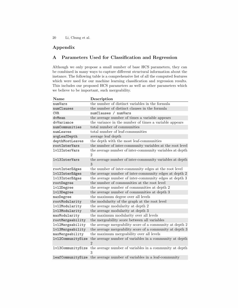
Although we only propose a small number of base HCS parameters, they canbe combined in many ways to capture different structural information about theinstance. The following table is a comprehensive list of all the computed featureswhich were used for our machine learning classification and regression results.This includes our proposed HCS parameters as well as other parameters whichwe believe to be important, such mergeability.
Name DescriptionnumVars the number of distinct variables in the formulanumClauses the number of distinct clauses in the formulaCVR numClauses / numVars
dvMean the average number of times a variable appearsdvVariance the variance in the number of times a variable appearsnumCommunities total number of communitiesnumLeaves total number of leaf-communitiesavgLeafDepth average leaf depthdepthMostLeaves the depth with the most leaf-communitiesrootInterVars the number of inter-community variables at the root levellvl2InterVars the average number of inter-community variables at depth
2lvl3InterVars the average number of inter-community variables at depth
3rootInterEdges the number of inter-community edges at the root levellvl2InterEdges the average number of inter-community edges at depth 2lvl3InterEdges the average number of inter-community edges at depth 3rootDegree the number of communities at the root levellvl2Degree the average number of communities at depth 2lvl3Degree the average number of communities at depth 3maxDegree the maximum degree over all levelsrootModularity the modularity of the graph at the root levellvl2Modularity the average modularity at depth 2lvl3Modularity the average modularity at depth 3maxModularity the maximum modularity over all levelsrootMergeability the mergeability score between all variableslvl2Mergeability the average mergeability score of a community at depth 2lvl3Mergeability the average mergeability score of a community at depth 3maxMergeability the maximum mergeability over all levelslvl2CommunitySize the average number of variables in a community at depth
2lvl3CommunitySize the average number of variables in a community at depth
3leafCommunitySize the average number of variables in a leaf-community

On the HCS of Practical SAT Formulas 21
Name DescriptionnumLeaves /
numCommunities
rootInterEdges /
rootInterVars
lvl2InterEdges /
lvl2InterVars
lvl3InterEdges /
lvl3InterVars
max(interEdges /
interVars)
the maximum interEdges / interVars ratio over alllevels
rootInterEdges /
rootCommunitySize
lvl2InterEdges /
lvl2CommunitySize
lvl3InterEdges /
lvl3CommunitySize
max(interEdges /
communitySize)
the maximum interEdges / communitySize ratio overall levels
rootInterVars /
rootCommunitySize
lvl2InterVars /
lvl2CommunitySize
lvl3InterVars /
lvl3CommunitySize
max(interVars /
communitySize)
the maximum interVars / communitySize ratio over alllevels
rootInterEdges /
rootDegree
lvl2InterEdges /
lvl2Degree
lvl3InterEdges /
lvl3Degree
rootInterVars /
rootDegree
lvl2InterVars /
lvl2Degree
lvl3InterVars /
lvl3Degree

22 Li, Chung et al.
B Scaling Studies: Inter-community Edges vs. Number ofVariables
In our scaling studies, we change the number of variables and observe that thescaling behaviour of the total number of inter-community edges in the formula isdifferent for different classes of instances. Log scale plots of this scaling behaviourfor each of the instance classes considered in this work are presented here:
log(# of variables)
root
inte
rcom
mun
ity e
dges
500
1000
5000
10000
50000
100 1000 10000 100000
agile
(a) Agile
log(# of variables)ro
ot in
terc
omm
unity
edg
es
100
1000
10000
100000
100 1000 10000 100000
verification
(b) Verification
log(# of variables)
root
inte
rcom
mun
ity e
dges
100
1000
10000
100000
1000000
50 100 500 1000 5000 10000 50000
crafted
(c) Crafted
log(# of variables)
root
inte
rcom
mun
ity e
dges
2000
4000
60008000
20000
40000
4000
6000
8000
1000
020
000
4000
060
000
8000
0
crypto
(d) Crypto
log(# of variables)
root
inte
rcom
mun
ity e
dges
1000
10000
100000
1000000
1000
2000
4000
6000
8000
1000
020
000
random
(e) Random

On the HCS of Practical SAT Formulas 23
C Theoretical Results
C.1 Embedding expanders in HCS graphs
We next show that a good enough HCS decomposition would disallow largeexpanders embeddable in the graph. Let us consider graphs with the followingrestrictions on HCS.
1. Small leaf size: all leaves are of size at most O(log n).2. Bounded community degree: for every community at every level, the number
of immediate sub-communities is bounded by O(log n).3. Small number of inter-community edges (the smaller the better).
The reason for the small leaf size condition is to avoid the counterexampleof Mull, Fremont, and Seshia [31]. The second condition, bounded communitydegree, avoids counterexamples in section C.3. The last property is needed toavoid the counterexample at the end of this section.
In the following, we use G to refer both to a family of graphs as well as aspecific representative of that family (the reason for the family is to be able totalk about asymptotic behaviour of parameters).
Claim. Suppose a graph G with |G| = n has a community decomposition intoC1, . . . , C` maximizing the modularity (flat, single-level decomposition). Let Hbe a subgraph of G, with |H| = f(n) for some f(n) ∈ O(n). Then either H isnot an expander, or the number of inter-community edges is Ω(f(n)), or thereexists a community containing a subgraph of H of size at least f(n)(1− o(1)).
Proof. Suppose that H is an expander graph of size f(n) with edge expansionh(H) = α, and let S be the largest subset of H which is within a single Ci (wlog,say S ⊆ C1). Suppose that |S| = δ · f(n) for some constant δ. Then the numberof edges out of C1 is at least α ·minδ, 1−δf(n), and thus the the total numberof inter-community edges is Ω(f(n)). If |S| = o(f(n)), then it is possible to splitcommunities C1 . . . Ct into 2 sets with roughly the same number of vertices ofH on each side (up to a subconstant factor); the number of edges of H goingacross this cut should be close to αf(n), again Ω(f(n)).
Theorem 3. Let G = Gn be a family of graphs. Let f(n) ∈ ω(poly(log n)),f(n) ∈ O(n). Assume that G has HCS with the number of inter-community edgeso(f(n)) for every community C of size at least Ω(f(n)) and depth is bounded byO(log n). Then G does not contain an expander of size f(n) as a subgraph.
Proof. Let H be a subgraph of G of size f(n). Let C be the smallest sub-community in the hierarchical decomposition of G containing at least (1−o(1))-fraction of H. Note that if H is an expander, then any subgraph of H on 1−o(1)vertices is also an expander.
First, since |H| ∈ ω(poly(log n)), C cannot be a leaf. Therefore, C it willbe partitioned into sub-communities C1 . . . C` by the hierarchical decomposi-tion. Since we assumed that C is the smallest community containing (1− o(1))

24 Li, Chung et al.
fraction of H and depth is O(log n), each sub-community of C can contain atmost a constant fraction of H. Then by claim C.1, since |C| ∈ Ω(f(n)) and soby assumption the number of inter-community edges in this decomposition isbounded by o(f(n)), H is not an expander.
One of the main measures of ”quality” of HCS is modularity value of thedecompositions throughout the hierarchy: the higher values correspond to bet-ter structural properties. Let us start by relating modularity to the number ofinter-community edges. Note that while both the definition of expander andmodularity are essentially relying on estimating how far the number of edgesacross the ”best” partition is from the expected value, the dependence on thesize of the communities is somewhat different.
First, to simplify our proof, consider decomposition into 2 communities; wecan do it thanks to the following claim.
Claim. [33] Suppose that C1 . . . Ct is a decomposition of C optimizing modu-larity. Then for some S = Ci1 , . . . , Ci` the partition into S and S maximizesmodularity among 2-partitions.
Corollary 1. For any graph G, the best modularity of a 2-partition is a lowerbound for the modularity of an optimal partition, with edges in the the best 2-partition a subset of inter-community edges in the optimal partition.
To simplify notation, for a set S ⊂ V , define vol(S) = Σv∈Sdeg(v). Leteout(C) be the set of edges leaving a community Ci, so ΣC∈P eout(C) is the setof all intercommunity edges in a partition P . Now, we can restate the formula formodularity of a partition P as follows, using the fact that ΣC∈P vol(C) = 2|E|:
Q(P ) = 1− 1
2|E|ΣC∈P eout(C)− 1
4|E|2ΣC∈P (vol(C))2
The optimal Q of a graph G is then Q = Q(G) = maxP Q(P ). Let Q2 =Q2(G) = maxP,|P |=2Q(P ) (that is, optimal modularity over 2-partitions). Notethat Q(G) ≥ Q2(G) for any G. Let P be a partition of G into a set S and itscomplement S; we will always assume, without loss of generality, that |S| ≤ |S|.Let |V | = n and |E| = m (not to be confused with the number of clauses in theformula for which G is a VIG). Then
Q(S, S) = 1− eout(S)/2m− eout(S)/2m− (vol(S)/2m)2 − (vol(S)/2|E|)2
= 1− eoutS/m−1
4m2(vol(S)2 + (2m− vol(S))2)
= vol(S)/m− vol(S)2/2m2 − eout(S)/m
=vol(S)
m(1− vol(S)/2m)− eout(S)/m
From there, we get that eout(S) = vol(S)(1−vol(S)/2m)−Q(S)m. Note thatsince Q2 = maxSQ(S, S), eout(S) = vol(S)(1−vol(S)/2m)−Q2m. Therefore,if vol(S)(1− vol(S)/2m)−Q2m = o(f(n)), then so is eout(S).

On the HCS of Practical SAT Formulas 25
C.2 HCS Avoids the Resolution Limit in Some Graphs
We prove Theorem 2, restated below more formally.
Theorem 2 (restated). There exists a graph G whose natural communitiesare of size log n and correspond to Ph(G), while P(G) consists of communities
of size√n/ log3 n.
We use as the separating graph G the ring of cliques example of [19], whichcan be built as follows. Start with a collection of q = n/c cliques C1, . . . , Cq,each of size c = log n. Fix a canonical vertex vi for each clique Ci. Add edgesbetween vi and vi+1, wrapping around at q. The number of vertices is n andthe number of edges is m = n
c
(c2
)+ n
c = n(c + 1)/2 + o(n). The degree of mostvertices is c− 1, except for the canonical vertices which have degree c+ 1. Thenatural partition of G into communities is the set of cliques C1, . . . , Cq.
We say that a subgraph of G preserves the cliques if for every clique, itcontains either all or none of its vertices. We say that a partition of G preservesthe cliques if every element of the partition preserves the cliques.
To prove that Ph(G) = C1, . . . , Cq we need the following two observations.
Lemma 1. Let H be a subgraph of H that preserves the cliques. Then any par-tition of H optimizing subgraph modularity preserves the cliques.
Proof. Let V1, . . . , Vk be a partition and assume that clique Ci contains verticesin at least two different sets Vj . We claim that the partition V1\Ci, . . . , Vk\Ci, Cihas greater modularity and that the number of split cliques decreases, thereforeiterating this procedure until no clique is split concludes the lemma.
To prove the claim, let Uj = Vj ∩Ci and note that the change in modularityis at least
2m∆Q ≥ −4
(1− (c+ 1)2
2m
)+∑j 6=j′
∑u∈Uj
∑v∈Uj′
(1− d(u)d(v)
2m
)(2)
≥ −4 +∑j 6=j′|Uj ||Uj′ |
(1− (c+ 1)2
2m
)(3)
≥ −4 +1
2
∑j 6=j′|Uj ||Uj′ | (4)
≥ −4 +1
4
∑j 6=j′,|Uj |>0,|U ′
j |>0
|Uj |+ |Uj′ | (5)
≥ −4 + c/4 > 0
Lemma 2. Let H be a subgraph of H that preserves the cliques. If H containsq ≥ 2 cliques, then any partition of H optimizing subgraph modularity containsat least 2 elements.

26 Li, Chung et al.
Proof. Let V1, V2 be the partition where the first half of the cliques in H arecontained in V1 and the rest in V2. The change in modularity with respect tothe singleton partition is at least
2m∆Q ≥ −2
(1− (c+ 1)2
2m
)+∑u∈V1
∑v∈V2
d(u)d(v)
2m(6)
≥ −2 + (cq/2)2(c− 1)2
2m= −2 +
n2c2
9nc> 0
We can now compute Ph(G) by induction, using the induction hypothesisthat every node of the hierarchical tree is a subgraph that preserves the cliques.The root is the whole graph G and trivially preserves the cliques. Every nodeof the hierarchical tree preserves the cliques, then by Lemma 1 all its childrenpreserve the cliques. This implies that all of the leaves preserve the cliques. How-ever, a leaf cannot consist of more than one clique, otherwise it would contradictLemma 2. It follows that all the leaves are single cliques as we wanted to show.
Next we prove that the partition optimizing modularity has large elements,for which we need the following observations.
Let V1, . . . , Vk be a partition that preserves the cliques. We define the oper-ation “move clique a to position b” as follows. Assume a < b. For a ≤ i < b weassign clique i to the set containing clique i+1, and clique b to the set containingclique a. Analogous if a > b.
Lemma 3. The modularity of G is maximized by a partition of contiguouscliques.
Proof. By Lemma 1 the partition consists of unions of cliques. Assume a setcontains non-contiguous cliques. Moving two intervals of cliques next to eachother increases the modularity, therefore we can keep repeating this procedureuntil the sets only consist of contiguous intervals.
In what follows we assume that n is large enough for it not to make it adifference when we treat variables as being continuous when they are in factdiscrete.
Lemma 4. The modularity of G is maximized by a partition of equal-sized ele-ments.
Proof. By Lemma 3 the partition consists of intervals of cliques. Assume intervalVa is smaller than interval Vb. Let Ci be an endpoint of Vb. Then assigning cliqueCi to Va and moving it next to an endpoint of Va increases the modularity,therefore we can repeat this procedure until the sets are balanced.
Lemma 5. The modularity of G is maximized by a partition with elements of
size√n/ log3 n.
On the HCS of Practical SAT Formulas 27
Proof. By Lemma 4 the partition consists of equal-sized intervals of cliques. Letk be the size of the partition and let q be the number of cliques in each block.The modularity is
2mQ = k
(qc(c− 1) + 2(q − 1)− 1
2m
(q2(c+ 1)2 + (7)
+ q(q(c− 1))(c+ 1)(c− 1) + (q(c− 1))2(c− 1)2))
(8)
= (n/cq)
(q(c2 − c+ 2)− 2− q2
2m
((c+ 1)2 + (c− 1)2(c+ 1) + (c− 1)4
))(9)
= (n/c)(c2 − c+ 2)− 2n/cq − nq
2mc
((c+ 1)2 + (c− 1)2(c+ 1) + (c− 1)4
)(10)
which is a function of the form a0 − a1q−1 − a2q and is maximized when its
derivative is 0 at point
q =
√a1a2≥
√2n/c
nc3/2m≥√
2n
c3(11)
This completes the proof of Theorem 2.
C.3 Justification for Parameter Choices and Lower Bounds for HCS
For a formula to have “good” HCS, we require that a number of parametersfall within appropriate ranges. One could hope that a single parameters of HCSmight be sufficient in order to guarantee tractability, while also capturing a suffi-ciently large set of interesting instances. A natural candidate parameter would behigh smooth modularity : The modularity of the VIG is large, and the decrease inmodularity from the parent to a non-leaf child in the HCS is sufficiently bounded.This captures the recursive intuition of HCS: each community should either bea leaf or should have a good partition into communities; this is closely related tothe average modularity at each level, which is a parameter used in our experi-ments. However, in this section we show that if we are after provable tractability,it is unlikely that a single parameter of HCS will suffice. In doing so, we motivateusing an ensemble of parameters as we have done in our experiments, as well asjustify why we have chosen many of the parameters that we have.
Formally, we show that combinations of the following ranges of parametersadmit formulas which are exponentially hard to refute in resolution.
– High Root Modularity : The modularity of G is sufficiently large.– High Smooth Modularity : The modularity of G is sufficiently large and the
modularity of every non-leaf node is bounded below by a function of its level.– Bounded Leaf Size: Each of the leaf-communities of the optimal HCS decom-
position is sufficiently small — in particular, of size O(log n).
28 Li, Chung et al.
– High Depth: There is a sufficiently deep path in the optimal HCS decompo-sition.
– Minimum Depth: There is a lower bound on the depth of every path in theoptimal HCS decomposition.
– Dense Inter-Community Edges: The optimal HCS decomposition has Ω(nε)inter-community edges between for all communities of size O(nε)
One finding that we would like to highlight is that in order to enure that the for-mula is tractable, the leaf-communities of the optimal HCS decomposition can-not be both large (of size ω(log n)) and unstructured; indeed, HCS says nothingabout the structure of the leaf-communities.
Finally, we note that we can still construct hard formulas which have “good”HCS parameters. However, the construction of these formulas is highly contrivedand non-trivial and we do not see a way to simplify them. Indeed, they are farmore contrived than the counterexamples to modularity given by [31]. We takethis as empirical evidence that instances with good HCS avoid far more hardexamples than formulas with high modularity.
Throughout, it will be convenient to make use of the highly sparse VIGsprovided by random CNF formulas. For positive integer parameters m,n, k, letF(m,n, k) be the uniform distribution on formulas obtained by picking m k-clauses on n variables uniformly at random with replacement. It is well knownthat for any k, the satisfiability of this F ∼ F(m,n, k) is controlled by the clausedensity ∆k := m/n: there is a threshold of ∆k after which F ∼ F(m,n, k) be-comes unsatisfiable with high probability. Furthermore, random k-CNF formulasnear this threshold (∆k = O(2k) suffices) require resolution refutations of size2n
ε
for some constant ε > 0 with high probability [13,5]. The VIG of such a for-mula is sparse (it has Θ(n) edges) and with high probability the maximum degreeis O(log n). Furthermore, with high probability F is expanding, and thereforethe edges are distributed roughly uniformly throughout the VIG.
For brevity, our arguments section will be somewhat informal; however, itshould be clear how to formalize them.
Root Modularity. Mull, Fremont, and Seshia [31] proved that having a highlymodular VIG does not suffice to guarantee short resolution refutations. To do so,they extended the lower bounds on the size of resolution refutations of randomk-CNF formulas [13,5] to work for a distribution of formulas whose VIGs havehigh modularity, thus showing the existence of a large family of hard formulaswith this property.
A much simpler proof of their result — albeit with slightly worse parame-ters — can be obtained as follows: Let F ∼ F(m,n, k) with k,m set appropri-ately so that F is hard to refute in resolution with high probability, and let F ′
be the formula obtained by taking t copies of F on disjoint sets of variables.It can be checked that the modularity of the partition of the VIG of F ′ whichhas t communities, one corresponding to each of the copies of F has modularity1− o(1/t). Setting t sufficiently large, we obtain a formula whose VIG has highmodularity. As each copy of F is on distinct variables, refuting F ′ is at least
On the HCS of Practical SAT Formulas 29
as hard as refuting F . Thus, a lower bound of 2Ω(nε) for some constant ε > 0follows from the known lower bounds on refuting F in resolution. If we let v = ntbe the number of variables of F ′ then this lower bound is of the form 2Ω((v/t)ε)
and is superpolynomial provided t = o(n/ log n). This argument also applies tohierarchical community structure.
Observe that each leaf-community of F ′ is a formula F on v/t variables whichis hard to refute in resolution. This shows that if we want to ensure polynomial-size resolution proofs, then we cannot allow the leaf communities of the HCSdecomposition to be both unstructured and large (of size ω(log n)). The simplestway to avoid this is to require the size of the leaf-community to be bounded byO(log n). However, in a later paragraphs we will show that this restriction is notsufficient on its own.
Root Modularity and Maximum Depth The previous example can be mod-ified in order to rule out requiring an upper bound on the depth and high smoothmodularity. We will use the simple observation the at the optimal communitystructure decomposition of t disjoint cliques on n vertices has t communities, onefor each clique. Furthermore, HCS will not decompose any of these cliques, andtherefore the optimal HCS has a single level and maximum depth assumption.
Let F ′ be the formula constructed in the previous example. We will modifyeach copy of F so that its VIG is a clique Kn. Let i ∈ [t], and for the ithcopy of F do the following: pick a variable xi 6= v∗i and note that there is adirection αi ∈ 0, 1 in which it can be set such that the complexity of refutingF (x = αi) in resolution is at most half the complexity of refuting F . Add anarbitrary clause of length n containing every variable in F such that x occurspositively if αi = 1 and negatively otherwise. Observe that the VIG of F is nowa clique.
After this process, the VIG of F ′ has t disjoint cliques. It remains to seethat F ′ is still hard to refute in resolution. This follows because applying therestriction which sets xi = αi for all i ∈ [t] leaves us with t disjoint copiesof F ′ which require 2Ω(nε) size resolution refutations, and because resolutioncomplexity is closed under restriction.
Smooth and Bounded Leaf Size. Next, we show that requiring the optimalHCS decomposition to have high smooth modularity and to have bounded leafsize is not sufficient in order to ensure small resolution refutations. Let F ∼F(m,n, 3) be a random 3-CNF formula with m set so that F is hard to refutein resolution whp. Let G be the VIG of F , which has Θ(n) edges and degreeO(log n) whp. Let p = O(log n) and Kp be a clique on p vertices. Let 2 ≤ t ≤ pbe any integer and let FK be any t-CNF formula on p variables such that everypair of variables occurs in some clause; this requires at most p2 clauses. Observethat the VIG of FK is Kp. Furthermore, observe that FK is satisfied by anytruth assignment that sets at least p− t+ 1 variables to true.
Using Kp and G we construct a family of formulas that is hard to refutein Resolution and whose VIG has the desired properties. Let G′ be the rooted

30 Li, Chung et al.
product of G and Kp, that is let v∗ be an arbitrary vertex of Kp, create n copiesof Kp, and identify the ith vertex of G with the vertex v∗ of the ith copy of Kp.
Next, we show that because G is sparse and each Kp is a clique, G′ hasmodularity which tends to 1 with n.
Lemma 6. Let G be a graph of order n, size m = Θ(n), and degree O(√n); let
Kp be a clique on p vertices with p = ω(1) and p = o(n); and let G′ be the rootedproduct of G and Kp. Then Q(G′) = 1− o(1).
Proof. Let m′ ≤ m+np2/2 be the number of edges of G′. Consider the partitionP given by the n copies of Kp. We have
Q(P ) ≥ np2
2m′
[1− (d+ p)2
2m′
]≥[1− m
m′
] [1− (d+ p)2
2m′
](12)
and m/m′ = o(1) because p = ω(1), while (d + p)2/2m′ = o(1) because d =O(√n) and p = o(n). Hence Q(G′) ≥ Q(P ) = 1− o(1).
As well, by a similar argument to the proof of Lemma 1, the optimal HCSdecomposition will preserve cliques at each level (i.e. none of the cliques Kp willbe decomposed during the HCS decomposition. Furthermore, by an argumentsimilar to Lemma 5, each node in the HCS decomposition will have too manychildren. Finally, observe that because the variables of the random CNF formulaF are distributed uniformly, the non-clique edges in G will be distributed ap-proximately uniformly between the cliques. Taken together, this implies that themodularity of every non-leaf node in the HCS cannot decrease too much com-pared to the modularity of its parent. In particular, we satisfy the high smoothmodularity condition.
It remains to show that we can construct a formula with the same VIG whichis hard to refute in resolution. Let F ′ be the formula obtained in the same way:begin with the formula F . Make n copies of FK and choose some vertex v∗ifrom the ith copy of Fk. Identify v∗i with xi, the ith variable of F . Observe thatthe VIG of F ′ is exactly G′. It remains to argue that F ′ is hard to refute inResolution. Let Vi be set of variables on which the ith copy of FK depends. Letρ ∈ 0, 1, ∗pn be the restriction which sets all variables in Vi \ v∗i to true for alli ∈ [n] and does not set each v∗i (that is ρ(v∗i ) = ∗ for all v∗i ). We claim thatF ′ ρ = F . Indeed, each clause in each FK depends on at least two variables,of which at least one is set to true because t ≥ 2. The only variables on whichF depends are v∗i for i ∈ [n], which have been left untouched; thus F ρ = F .The lower bound on F ′ follows from the lower bound on 2Ω(nε) lower bound onF together with the fact that the complexity of resolution proofs is closed underrestriction.
Deep, Smooth, Bounded Leaf Size. We extend the previous example toshow that if, in addition to the previous restrictions, we require the HCS de-composition have high depth, then this is still insufficient to guarantee shortresolution proofs. To see this, let F ′ be the formula constructed in the previous

On the HCS of Practical SAT Formulas 31
example, and let F ′′ be a formula containing only positive literals and whoseVIG satisfies smooth HCS, bounded leaf-community size, and whose optimalHCS decomposition has a sufficiently deep root-to-leaf path. Note that such aformula F ′′ exists if and only if there exists a formula satisfying these proper-ties with no restriction on the polarity of the literals. Therefore, we can assumethe existence of F ′′, as otherwise this set of parameters does not capture anyinstances and is therefore not useful.
We claim that the VIG corresponding to F ′ ∧ F ′′ will satisfy their sharedproperties. First, observe that F ′ ∧ F ′′ has high modularity: the modularity ofboth F ′ and F ′′ is high by assumption and therefore the partition which is theunion of the maximum modularity partitions of F ′ and F ′′ will have high mod-ularity. Furthermore, because F ′ and F ′′ are disjoint, the HCS decompositionwill never never put (a part of) both of these formulas in the same community.Thus, the maximum modularity partition is the union of the maximum parti-tions of F ′ and F ′′. From then onwards, because F ′ and F ′′ are smooth, theHCS decomposition of F ′ ∧ F ′′ will be smooth. As well, because F ′′ has a deepdecomposition, this implies that the decomposition of F ′∧F ′′ will also contain adeep path. Finally, because F ′′ is satisfiable and F ′ requires exponential lengthrefutations in resolution, F ′ ∧ F ′′ does as well.
Lower bounds when the number of inter-community edges is large.Finally, we show that, under the assumption that each large community has anon-negligible fraction of inter-community edges, we can construct a hard for-mula satisfying most “good” HCS parameters. We note that the requirement onthe inter-community edges is fairly weak and we believe that it can be weakened.
Consider a formula F with a VIG G such that its hierarchical decompositionhas Ω(nε) inter-community edges for all communities of size O(nε); suppose alsothat the community degree of F is a constant c. We show that it is then possibleto embed a graph of a sparse hard formula of size O(nε) into the graph of F ,and construct a formula with the same VIG so that refuting this new formulaamounts to refuting the sparse hard formula.
Let FH be a (family of) hard formulas on n′ = nε variables with a constantclause width k such as each variable occurs in constantly many clauses ∆; forexample, FH could be a Tseitin formula on a 3-regular expander. We choose FHto be such that VIG of FH is a d-regular expander, where d = ∆ · w; this issatisfied by formulas resulting from the Tseitin contradictions on expanders.
Let F be a (family of) easy formulas with a VIG GF with “good” HCSparameters except that its hierarchical decomposition has Ω(nε) ≥ bnε inter-community edges for all communities of size O(nε), and such that the degreeof vertices in its VIG is at least D for some large enough D. Note that thenumber of communities of this size is at least 2n1−ε, so the average number ofinter-community edges out of each vertex of GF is at least 2b = 2n1−ε · bnε/n.To simplify calculations, take D ≥ 4d+ 4b (note that D can still be a constant,just a larger constant than d).
Now, add nε new vertices to G, placing each of them in a separate leaf ofthe hierarchical decomposition of GF . Associate each of these vertices with a

32 Li, Chung et al.
variable of FH , and add edges corresponding to clauses of FH ; call the resultingsubgraph GH . Now, for each leaf containing a new variable v∗i , add v∗i to enoughclauses within this leaf to bring the degree of v∗i up to D (here, assume thatthese leaves are of size at least D). Finally, create a new formula F ′ = F+ ∧FH ,where F+ is F with all negations removed (that is, every literal of F+ is positiveand so F+ is trivially satisfiable). Therefore, to refute F ′ it is necessary to refuteFH . If FH is a Tseitin contradiction on a 3-regular expander, then the size of itsresolution proof is 2Ω(n′) = 2Ω(nε) [6,45].
Claim. HCS properties of the VIG of F ′, GF ′ , are indistinguishable from thoseof the VIG of F .
Proof outline. First, consider the root of the hierarchical decomposition, thatis, the first decomposition of GF ′ . We can show that the optimal partition ofGF ′ is very close to the optimal partition of GF because new vertices form avery small part of every community, and every vertex of GH has many moreedges to the vertices outside of GH in GF ′ than to vertices within GH . Letcommunity degree be c and suppose the expansion of GH is α; then, in theworst case, the decomposition will contribute c(c − 1)αnε/2c = c−1
2 αnε edges.But as we assumed that the number of edges is already O(nε), this will add atmost a constant factor to the total number of inter-community edges at the rootlevel. Now we can repeat this argument for the subcommunities, which, sincevertices were selected randomly, with high probability will contain the numberof variables of GH proportional to their size, and have a diminishing fraction ofedges of GH .