Embed Size (px)
Citation preview

On the Geometry of the
Spin-Statistics Connection
in Quantum Mechanics
Dissertationzur Erlangung des Grades
,,Doktor der Naturwissenschaften“am Fachbereich Physik
der Johannes Gutenberg-UniversitatMainz
vorgelegt vonAndres Reyesgeb. in Bogota
Mainz 2006

1. Gutachter: Prof. Dr. N. Papadopoulos2. Gutachter: Prof. Dr. F. Scheck

Zusammenfassung
Das Spin-Statistik-Theorem besagt, dass das statistische Verhalten eines Systems vonidentischen Teilchen durch deren Spin bestimmt ist: Teilchen mit ganzzahligem Spinsind Bosonen (gehorchen also der Bose-Einstein-Statistik), Teilchen mit halbzahligemSpin hingegen sind Fermionen (gehorchen also der Fermi-Dirac-Statistik). Seit demursprunglichen Beweis von Fierz und Pauli wissen wir, dass der Zusammenhang zwi-schen Spin und Statistik aus den allgemeinen Prinzipien der relativistischen Quanten-feldtheorie folgt.
Man kann nun die Frage stellen, ob das Theorem auch dann noch gultig bleibt, wennman schwachere Annahmen macht als die allgemein ublichen (z.B. Lorentz-Kovarianz). Es gibt die verschiedensten Ansatze, die sich mit der Suche nach solchenschwacheren Annahmen beschaftigen. Neben dieser Suche wurden uber viele Jahrehinweg Versuche unternommen einen geometrischen Beweis fur den Zusammenhangzwischen Spin und Statistik zu finden. Solche Ansatze werden haupt-sachlich, durch den tieferen Zusammenhang zwischen der Ununterscheidbarkeit vonidentischen Teilchen und der Geometrie des Konfigurationsraumes, wie man ihnbeispielsweise an dem Gibbs’schen Paradoxon sehr deutlich sieht, motiviert. Ein Ver-such der diesen tieferen Zusammenhang ausnutzt, um ein geometrisches Spin-Statistik-Theorem zu beweisen, ist die Konstruktion von Berry und Robbins (BR). DieseKonstruktion basiert auf einer Eindeutigkeitsbedingung der Wellenfunktion, die Aus-gangspunkt erneuerten Interesses an diesem Thema war.
Die vorliegende Arbeit betrachtet das Problem identischer Teilchen in der Quanten-mechanik von einem geometrisch-algebraischen Standpunkt. Man geht dabei voneinem Konfigurationsraum
�mit einer endlichen Fundamentalgruppe � � ���
aus.Diese hat eine Darstellung auf dem Raum � � ���
, wobei �� die universelle Uberlagerungvon
�bezeichnet. Die Wirkung von � � ���
auf �� induziert nun eine Teilung von � � ���in disjunkte Moduln uber � ���
, die als Raume von Schnitten bestimmter flacher Vek-torbundel uber
�interpretiert werden konnen. Auf diese Weise lasst sich die geo-
metrische Struktur des Konfigurationsraums�
in der Struktur des Funktionenraums� � ���kodieren. Durch diese Technik ist es nun moglich die verschiedensten Ergeb-
nisse, die das Problem der Ununterscheidbarkeit betreffen, auf klare, systematischeWeise zu reproduzieren. Ferner findet man mit dieser Methode eine globale For-mulierung der BR- Konstruktion. Ein Ergebnis dieser globalen Betrachtungsweise ist,dass die Eindeutigkeitsbedingung der BR-Konstruktion zu Inkonsistenzen fuhrt. Einweiterfuhrendes Proposal hat die Begrundung der Fermi-Bose-Alternative innerhalbunseres Zugangs zum Gegenstand.


Contents
1. Introduction 1
1.1. Motivation . . . . . . . . . . . . . . . . . . . . . . . . . . . . . . . . . . . . 1
1.2. On the present work . . . . . . . . . . . . . . . . . . . . . . . . . . . . . . 8
2. Quantization on multiply-connected configuration spaces 12
2.1. Motivation . . . . . . . . . . . . . . . . . . . . . . . . . . . . . . . . . . . . 12
2.2. Canonical Quantization from Group Actions . . . . . . . . . . . . . . . . 15
2.2.1. Preliminary remarks . . . . . . . . . . . . . . . . . . . . . . . . . . 15
2.2.2. From CCR to group actions and back . . . . . . . . . . . . . . . . 19
2.2.3. Representations of the canonical group . . . . . . . . . . . . . . . 26
3. G-spaces and Projective Modules 29
3.1. Equivariant bundles . . . . . . . . . . . . . . . . . . . . . . . . . . . . . . 29
3.2. Equivariant trivial bundles . . . . . . . . . . . . . . . . . . . . . . . . . . . 33
3.3. Projective Modules . . . . . . . . . . . . . . . . . . . . . . . . . . . . . . . 35
3.4. Decomposition of � � . . . . . . . . . . . . . . . . . . . . . . . . . . . . 40
4. The spin zero case 52
4.1. �� as Configuration Space . . . . . . . . . . . . . . . . . . . . . . . . . . . 52
4.1.1. Line Bundles over �� . . . . . . . . . . . . . . . . . . . . . . . . . . 52
4.1.2. Angular Momentum coupled to a Magnetic Field . . . . . . . . . 56
4.2. � � as Configuration Space . . . . . . . . . . . . . . . . . . . . . . . . . . 58
4.2.1. Line bundles over � � . . . . . . . . . . . . . . . . . . . . . . . . . 58
4.2.2. �� �� equivariance . . . . . . . . . . . . . . . . . . . . . . . . . . 63
4.2.3. Two Identical Particles of Spin Zero . . . . . . . . . . . . . . . . . 67
i

Contents
5. Applications to the Berry-Robbins approach to Spin-Statistics 69
5.1. Review of the construction . . . . . . . . . . . . . . . . . . . . . . . . . . . 70
5.2. The transported spin basis and projectors . . . . . . . . . . . . . . . . . . 75
5.3. Single-valuedness of the wave function . . . . . . . . . . . . . . . . . . . 78
6. Further developments 85
6.1. �� ��� and Spin . . . . . . . . . . . . . . . . . . . . . . . . . . . . . . . . . 86
6.2. Exchange . . . . . . . . . . . . . . . . . . . . . . . . . . . . . . . . . . . . . 89
A. G-Spaces 95
ii

1. Introduction
1.1. Motivation
Being a consequence of the general principles of relativistic Quantum Field Theory, theSpin-Statistics theorem has found rigorous proofs in the context of axiomatic, as wellas of algebraic Quantum Field Theory [Fie39, Pau40, LZ58, SW00, DHR71, DHR74,GL95, DS97]. In spite of many efforts, this has not been the case in non relativisticQuantum Mechanics. A proof of the Spin-Statistics theorem, which does not rely asheavily on concepts of relativistic Quantum Field Theory(QFT) as the established ones,is something desirable, for several reasons. There are many examples of phenomenataking place outside the relativistic realm (one could think of Bose-Einstein Condensa-tion, Superconductivity or the Fractional Quantum Hall Effect as relevant ones, not tomention the striking consequences of Pauli’s Exclusion Principle as the prediction of“exchange” interactions, or the explanation of the periodic table) which depend essen-tially on the Spin-Statistics relation for its description.
Furthermore, a proof based on assumptions which are different from the standard onescould also be of benefit for the understanding of QFT itself. For instance, a proof whichdoes not make use of the full Lorentz group could provide hints towards the under-standing of Spin-Statistics in more general situations, such as theories where a back-ground gravitational field is present� , or theories on non-commutative space-times.
The idea that the observed correlation between Spin and Statistics may, perhaps, bederived without making use of relativistic QFT is not a new one. Much work has beendevoted to the point of view that quantum indistinguishability, if correctly incorporatedinto quantum theory, might lead to a better understanding of Spin-Statistics. Mostof the work in this direction is based on formulations where the quantum theory of asystem of indistinguishable particles is obtained from a quantization procedure, whosestarting point is a classical configuration space.
In one of the first works of this kind, Laidlaw and DeWitt found out[LD71] that whenapplying the path integral formalism to a system consisting of a finite number of non-relativistic, identical spinless particles in three spatial dimensions, the topology of�
Although it is possible to generalize the proofs on Minkowski space to curved background space-times[Ver01], here we are interested in alternative approaches, of geometric nature.
1

1. Introduction
the corresponding configuration space imposes certain restrictions on the propagator.From this, they were able to deduce that only particles obeying Fermi or Bose statisticsare allowed (this Fermi-Bose alternative is an input in the standard proofs of axiomaticQFT).
Leinaas and Myrheim considered a similar situation in [LM77], in an analysis thatwas motivated by the relevance of indistinguishability to Gibbs’ paradox. They repro-duced the results of [LD71] by obtaining the Fermi-Bose alternative in three dimen-sional space for spinless particles. But, in addition, they also found that in one and twodimensions the statistics parameter could, in principle, take infinitely many values. Inthat same work, they remarked that their results could provide a geometrical basis fora derivation of the Spin-Statistics theorem.
A lot of work based on this kind of “configuration space approach” has been done sincethen, in an effort to find a simpler proof of the Spin-Statistics theorem, in comparisonto the relativistic, analytic ones.
Usually, such attempts are based on the point of view that, in non relativistic QuantumMechanics, indistinguishability, together with the rotational properties of the wavefunction describing a system of identical particles, are the physical concepts lying atthe core of the problem. There are several reasons that, from a theoretical perspective,really seem to justify such a standpoint. First of all, spin is an intrinsic property of aparticle which is closely related to spatial rotations: For example, just because of thedefinition of spin in terms of � � ��� representations, the wave function of a particle ofspin � changes its phase by a factor ����� under a �! rotation. The factor �� ��� isindeed a quantity that can be directly measured from the interference pattern (i.e. asa relative phase) of a two-slit-type experiment with neutrons where one of the beamsis subject to a magnetic field [Ber67, WCOE75]. The change in the sign of the wavefunction is then due to precession of the neutrons in the region where the magneticfield is present and provides a clear experimental evidence of the rotational proper-ties of the wave function (of a fermion, in this case). The fact that this phase is thesame as that defining the statistics of a system of identical particles of spin � , could beconsidered as a hint pointing towards a simple physical explanation of Spin-Statistics.This point of view is partially substantiated by the work of Finkelstein and Rubinstein[FR68] on a kind of topological Spin-Statistics theorem. Here, exchange of two identicalobjects is really correlated with the �! rotation of one of them, only that the objectsunder consideration are extended ones, known as kinks, or topological solitons. In theFinkelstein-Rubinstein approach, one considers configurations of non-linear classicalfields. The fields are assumed to take values on a given, fixed manifold and to satisfysome boundary conditions (e.g., fields must take a constant value at spatial infinity).The space of all fields -the configuration space- can be given a suitable topology, thusallowing a classification of fields according to the connected component they belongto. A field differing from the constant one only in a bounded region of space is referredto as a localized kink and it can carry a “charge”, according to the component it belongsto. Such kinks are objects that, because of the existence of a notion of localization, maybe regarded as “extended-” (in contrast to “point-”) particles. In a few words, the main
2

1.1. Motivation
result of Finkelstein-Rubinstein is that an exchange of two identical kinks is equivalent(in the sense of homotopy) to a "# rotation of one of them. It must be emphasized thatin their proof, the idea of pair creation/annihilation is introduced and used extensivelyin order to establish the mentioned equivalence.
Although the work of Finkelstein-Rubinstein appeared almost a decade before thoseof Leinaas-Myrheim or of Laidlaw-DeWitt, it has not been possible to obtain analo-gous results for systems of point particles, at the quantum level. A proposal, inspiredin part by the results of Finkelstein-Rubinstein, has been put forward by Balachan-dran et.al. in a series of papers [BDG$90, BDG$93] where configuration spaces forpoint particles allowing for the possibility of pair creation and annihilation are consid-ered. In this approach, spin is modelled (within these classical configuration spaces)by means of “frames” which are attached to the particles. Due to the possibility ofpair creation/annihilation, the configuration space admits configurations of any num-ber of particles and antiparticles, thus being highly non trivial from the mathematicalpoint of view. The topology given to the configuration space allows for coincidencesof particles and antiparticles, but in a restricted way. The restrictions for arbitrary co-incidences are dictated by consistency conditions, and also by analogies with the topo-logical approach of Finkelstein-Rubinstein for kinks. An independent approach, usinga similar kind of configuration space (with a different coincidence condition and a dif-ferent topology) has been worked out by Tscheuschner [Tsc89]. A drawback commonto these approaches is that, although the idea of pair creation/annihilation is includedat the level of the classical configuration space, there is no clear interpretation of theresults in terms of Quantum Field Theory. The fact that these configuration spaces ad-mit an arbitrary number of particles also makes an interpretation in terms of QuantumMechanics a difficult task. Also, since the configuration space is not a differentiablemanifold, it is not clear how questions about connections and parallel transport, whichare used to define, for example, the momentum operator or the statistics parameter (asa holonomy), can be reformulated.
It has been suggested [Tsc89, BDG$93] that these configuration spaces may be obtainedfrom the Hilbert space of the quantum theory by exploiting the projective nature of thespace of pure states. Unfortunately, the argumentations -in this respect- remain at aheuristic level.
In any case, once the topology of the configuration space upon which quantization is tobe carried out becomes non-trivial (as a consequence of quantum indistinguishability,or otherwise) a careful consideration of the mathematical aspects of the theory becomesnecessary.
In order to understand this last point and to put it in perspective, let us recall that sincethe advent of Gauge Theories to Particle and High Energy Physics in the fifties and the“discovery” of the deep mathematical concepts underlying the Gauge Principle[WY75],the mathematical theory of fiber bundles and connections has played an essential rolein the formulation and understanding of physical theories of the fundamental interac-tions. Modern Differential Geometry and Topology have played a crucial role for the
3

1. Introduction
understanding of fundamental issues as, for example, quantization of Gauge Theories,anomalies and renormalization, topological effects as solitons, instantons, monopoles,non-trivial vacua and many others.
In most cases, the use of these mathematical structures is mainly restricted to the classi-cal part of the theory. Just to give an example, in the quantization of Gauge Theories, athorough understanding of the geometry of constrained Hamiltonian systems is veryimportant for the quantization of the theory. In contrast to this, the presence of a kindof “Gauge Principle” is inherent to Quantum Theory. Indeed, the original intention ofH. Weyl when using his “Eichprinzip” was to obtain a unification of General Relativityand Electromagnetism by means of a re-scaling of the metric. The (conformal) expo-nential factor responsible for the change in scale was real, and as is well known, it wasshown by Einstein that the proposal was not viable. Soon after that, it was recognizedby London that Weyl’s ideas really made sense, but not without substantial changes:The exponential factor had to be actually chosen as complex, a phase factor, relatednot to the classical theories but to the quantum mechanical wave function. The conse-quences of this fact -the gauge freedom of the wave function- are widely known, withmany interesting applications. The geometric character of the quantum mechanicalphase can be clearly recognized in situations like, for example, the Aharanov-Bohm ef-fect. Also widely known are geometric phases [Kat50, Ber84], whose geometric naturewas originally pointed out by Simon [Sim83]. It is in this context, that of the geometryof quantum states in non-relativistic Quantum Mechanics, that the Spin-Statistics prob-lem fits in. When the topology of the configuration space is complicated enough, newpossibilities for the realization of quantum states appear. Indeed, the whole scheme ofquantization by means of a “Correspondence Principle” works so nicely for the theoryof, say, one electron in three-dimensional Euclidean space, just because the topologyand geometry of the configuration space are, in a certain sense, trivial. Then, as a con-sequence of the Stone von Neumann uniqueness theorem, it is unnecessary to look forrealizations of quantum states apart from the usual ones, namely in the Hilbert space%& '( ) *
. The fact that the standard canonical commutation relations can be representedas operators in this space can be traced back to the existence of a transitive abeliangroup of transformations [Ish84]. But as soon as one considers a more general typeof configuration space, even the application of the Correspondence Principle becomesan issue by itself, because in this case, a suitable analog of the canonical commutationrelations must be found. Since the representation of the resulting operators might takeplace in a space which is not a space of functions on the configuration space, one canin this way see why other possibilities for the realization of quantum states becomepossible and, in some cases, even necessary.
For the understanding of these situations, a thorough mathematical analysis becomesnecessary and indeed can, in many cases, give very concrete answers. For exam-ple, in the case of Quantum Mechanics of spinless particles on a (possibly multiply-connected) configuration space, which has been discussed extensively in the literature,one has a general result, which can be stated as follows:
4

1.1. Motivation
1.1.1. Theorem (cf.[LD71]). Let + be the manifold that corresponds to the classical configu-ration space of a spinless particle. Then, the inequivalent quantizations of this system are inbijective correspondence with the one dimensional unitary representations of the fundamentalgroup of +.
Let us make a few comments about this result.
, Since no spin is being considered, the wave function takes values on a one-dimensional vector space. This vector space might vary with the coordinatesof the configuration space.
, We do not specify, for the moment being, the specific quantization approach(canonical, path integral, etc.). Since the only input is a configuration space, wecan only face the kinematical part of the problem. Hence, inequivalent quanti-zations here refers to the different choices for the Hilbert space representationof the theory: There might be several ones, which fall in classes that could betermed “superselection sectors” and that can be put in bijective correspondencewith topological invariants of the configuration space. A complete quantizationmust also include a classical dynamical principle as input.
, The results of Laidlaw-DeWitt and Leinaas-Myrheim can be regarded as a partic-ular case of 1.1.1: Define, for a system of - particles in . spatial dimensions,/+ 01 2 3 4 5 5 5 4 2 36 78 9: ;times
<= >(1.1.1)
where= 1 ?@A B > C C C > AD E F A G 1 AH > for at least some pair @I > J E> I K1 J L
denotes theset of configurations where two or more particles coincide. Since configurationsdiffering only by a permutation of particles are considered the same, one has anequivalence relation @A B > C C C > AD E M @AN OBP > C C C > AN O: P E (with Q R S: any permuta-tion of the indices ?T> C C C > - L
). The configuration spaces considered in references
[LD71] and [LM77] are obtained from/+ by taking the quotient with respect to
this equivalence relation:
+ 01 /+US: C(1.1.2)
One can show that, for . V W, X B @+E M1 S: , so that there are only two possibilities,corresponding to the two characters of S: . For . 1 Y it is well known that X B @+Eis isomorphic to Artin’s braid group Z: [Art47]. This leads to new possibilities,anyonic statistics [Wil82]. For systems obeying this kind of statistics, the statisticsparameter is not a sign, as in the Fermi or Bose cases, but a phase [G\ .
The application of theorem1.1.1 to the case of identical spinless particles is of particularrelevance, since the imposition of a symmetrization postulate becomes, in this case,unnecessary: The two possible statistics, the fermionic and the bosonic one, arise as
5

1. Introduction
a direct consequence of the non-trivial topology of the configuration space and thusof indistinguishability. To prove the Spin-Statistics theorem in this particular case, itwould be necessary to show that only bosonic statistics is allowed. An attempt to provethis, under some continuity assumptions for the wave function, has been carried outby Peshkin [Pes03b].
The possibility of using a result analogous to theorem 1.1.1 for non vanishing spinseems even more remote, mainly for two reasons. Firstly, whereas in the spinless casethe quantum theory is obtained from a quantization procedure, for non-vanishing spinthere is no classical theory to start with. One can adopt the point of view that the zero-spin case, for which quantization poses no problem, provides the justification for theuse of vector bundles over the classical configuration space in order to define the wavefunction and then introduce spin by considering bundles with fibers with a dimensioncorresponding to the given value of the spin. But then, because the vector bundlesinvolved in these cases are of higher rank, the restrictions imposed by the topology ofthe configuration space are not as strong as in the spin zero case. In fact, even a rigorousderivation of the Fermi-Bose alternative for nonzero spin is still lacking (some remarksand suggestions were already made in [LM77]). This is certainly a necessary step inorder to, eventually, prove a Spin-Statistics theorem in this context.
The case of general spin has recently been considered by Berry and Robbins, who in[BR97] have provided an explicit construction, in which the quantum mechanics of twoidentical particles is formulated along the lines described in [LM77]. Let us explain insome detail the construction of [BR97] (henceforth referred to as the BR-construction),in order to point out some features that have served as the starting point for the presentwork and, at the same time, in order to motivate the approach that will be developedin the following chapters.
The BR approach is motivated, in part, by the idea that there is an unsatisfactory fea-ture in the usual treatment of indistinguishability in non relativistic QM, namely, thatthe wave function of a system of identical fermions is not single-valued, in the sensethat under the exchange of two particles it changes its sign. Since, because of indistin-guishability, this exchange has no physical meaning, there should be no change at all.This amounts to the requirement that the wave function should be defined on a con-figuration space where indistinguishability is already incorporated, i.e., the space ] ofeqn. (1.1.2). Although the idea of working with wave functions defined on this quo-tient space is implicit in their work, Berry and Robbins’ construction is really carried
out on ] (as defined in eq. (1.1.1)), a configuration space of distinguishable particles.In this way, they avoid the use of mathematical concepts that would be necessary oth-erwise.
The construction was originally proposed for the special case of two particles of spin _ .The basic idea consists in replacing the usual spin states `a b c de f `a b c ge, by position-dependent ones: `a b c de f `a b c g e hi d b ig j. This is the only way one can impose single-valuedness (in the sense explained below, see equation (1.1.5)) and still retain Pauli’sexclusion principle.
6
1.1. Motivation
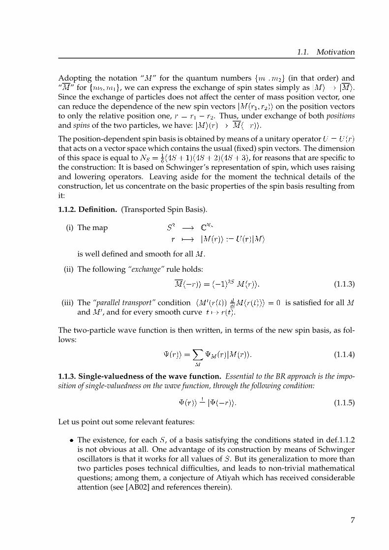
Adopting the notation “k ” for the quantum numbers lm n o m p q (in that order) and“k ” for lm p o m nq, we can express the exchange of spin states simply as rk s t rk s.Since the exchange of particles does not affect the center of mass position vector, onecan reduce the dependence of the new spin vectors rk uvn o vp ws on the position vectorsto only the relative position one, v x vn y vp . Thus, under exchange of both positionsand spins of the two particles, we have: rk s uv w t rk uyv ws.The position-dependent spin basis is obtained by means of a unitary operator z x z uv wthat acts on a vector space which contains the usual (fixed) spin vectors. The dimensionof this space is equal to {| x n} u~� � �wu~� � �wu~� � �w, for reasons that are specific tothe construction: It is based on Schwinger’s representation of spin, which uses raisingand lowering operators. Leaving aside for the moment the technical details of theconstruction, let us concentrate on the basic properties of the spin basis resulting fromit:
1.1.2. Definition. (Transported Spin Basis).
(i) The map� p yt � ��v �yt rk uv ws �x z uv w rk s
is well defined and smooth for all k .
(ii) The following “exchange” rule holds:
rk uyv ws x uy�wp| rk uv ws � (1.1.3)
(iii) The “parallel transport” condition �k � uv u� ww r ��� k uv u� wws x � is satisfied for all kand k �, and for every smooth curve
� �t v u� w.The two-particle wave function is then written, in terms of the new spin basis, as fol-lows:
r� uv ws x �� �� uv w rk uv ws � (1.1.4)
1.1.3. Single-valuedness of the wave function. Essential to the BR approach is the impo-sition of single-valuedness on the wave function, through the following condition:
r� uv ws �x r� uyv ws � (1.1.5)
Let us point out some relevant features:
� The existence, for each�
, of a basis satisfying the conditions stated in def.1.1.2is not obvious at all. One advantage of its construction by means of Schwingeroscillators is that it works for all values of
�. But its generalization to more than
two particles poses technical difficulties, and leads to non-trivial mathematicalquestions; among them, a conjecture of Atiyah which has received considerableattention (see [AB02] and references therein).
7

1. Introduction
� In the original proposal of BR, the sign in eq. (1.1.3) was assumed to be of the form�� ���and the conjecture was made that any basis satisfying the three properties
stated in definition 1.1.2 would have to satisfy�� ��� � ������
. The assertion ofthis conjecture was later found not to be true. Counterexamples have been givenin [BR00].
� In any case, for 2 particles the BR construction, using Schwinger’s oscillatorsmodel, gives the correct sign, and this for every value of � . It is therefore aninteresting matter to try to find the reason (in case there is one) for this.
� A direct consequence from eq. (1.1.5), when the spin vectors satisfy conditions(i)-(iii) from definition 1.1.2, is the relation � ��¡ � � ������ � �¡ �
, between thecoefficient functions. This could, in principle, be interpreted as the usual form ofthe Spin-Statistics relation ¢, but only if the conjecture about the sign in eq. (1.1.3)had turned out to be true.
1.2. On the present work
Having discussed the basic ideas that serve as motivation for the present thesis, wenow turn to a brief description of the method and techniques that have been used inour study of the Spin-Statistics problem.
In the last years, the BR proposal has given place to a renewed discussion of the Spin-Statistics problem, perhaps due to the fact that, in contrast to other approaches, whatthey present is a very concrete model which can be computed and also to the fact thatthe construction gave the correct connection between Spin and Statistics. Nevertheless,the existence of alternative constructions and the use of Schwinger’s oscillators in theoriginal one tend to obscure the real meaning of a “transported” spin basis. It wouldtherefore be interesting to find a method which, while keeping the concreteness, alsoleads to a better understanding of the problem.
For instance, although the motivation for the imposition of single-valuedness as a wayto include indistinguishability in the formalism is clear, its implementation by meansof eq.(1.1.5) is not. Let us explain this in more detail.
In the BR construction, the wave function is implicitly considered as a section of a vec-tor bundle, whose basis is supposed to be the physical configuration space £. As iswell known, it is not possible in general to represent a section by means of a singlefunction: The eventual non triviality of the bundle where it is defined makes the useof local trivializations necessary. A consequence of this is that, in order to recover a sec-tion as a whole, one needs several functions, one for each trivializing neighborhood.Thus, at every point on the basis manifold, the section will take (apparently) as many¤
First one has to show that these functions satisfy the same differential equation as the usual ones, see[BR97]
8

1.2. On the present work
values as there are trivializing neighborhoods covering that point. It should be em-phasized that this “multiple-valuedness” is only something apparent. A section is -inthe same way as a function- a map, which to each point on the basis manifold assignsa unique value on a vector space. The difference with a section is that the vector spacemight be different for every point. Now, as shown in this work, the equivalence be-tween projective modules and vector bundles [Ser58, Swa62] can be used as a tool inorder to obtain an algebraic characterization of certain vector bundles related to the
configuration spaces ¥ and ¦¥. More concretely, it will be shown that it is possible torepresent a section defined on a bundle over ¥ as a (possibly vector-valued) function
defined on ¦¥. Since the resulting function is not anymore defined on the physicallycorrect configuration space, its value now depends on the ordering of the particles andit is not necessarily invariant under exchange of them (it must, though, be equivari-ant). Thus, the imposition of strict invariance under exchange of particles for a wavefunction defined on §¥ as a vector-valued function seems not to be the most adequateform to incorporate indistinguishability into the theory. This point will be worked outin detail in chapter 5, where a comparison with the Berry-Robbins approach will bemade.
In this work (some of which results can be found in [PPRS04]), we will therefore studythe Spin-Statistics problem by making use of (some notions of) the theory of projectivemodules as an alternative, equivalent description of vector bundles. While from themathematical point of view the descriptions of vector bundles in the usual differential-geometric language and in terms of projective modules are completely equivalent (asasserted by the well known Serre-Swan theorem[Ser58, Swa62]) from the point of viewof our purposes, a description in terms of modules will be, at some points, much moreconvenient. The proposal to study the Spin-Statistics problem using projective mod-ules was made in [Pas01]. In the present thesis, it will be further developed, so as to bein a position to study the case of an arbitrary number of particles. The consideration ofthe symmetries of the problem will also play an important role in this work. In this re-spect, an approach in the spirit of [HPRS87] will be followed, mainly by considerationof the different group actions involved.
In order to illustrate how these concepts can be used to study the Spin-Statistics prob-lem, let us consider the spin basis of the BR-construction, in the special case of ¨ © ª«¬.There are, in this case, four physical, position dependent spin states, that are obtainedby application of an unitary operator ®¯ ° to the fixed ones. The resulting spin statescan be written as a linear combination of ten vectors ±² ³´ µ ¶ ¶ ¶ µ ±² ³· ´. The first four coin-cide with the fixed spin states,
±¸ µ ¸ ´ © ±²³´ µ±¹ µ ¹´ © ±²º ´ µ±¸ µ ¹´ © ±²» ´ µ±¹ µ ¸ ´ © ±²¼ ´ ¶
9
1. Introduction
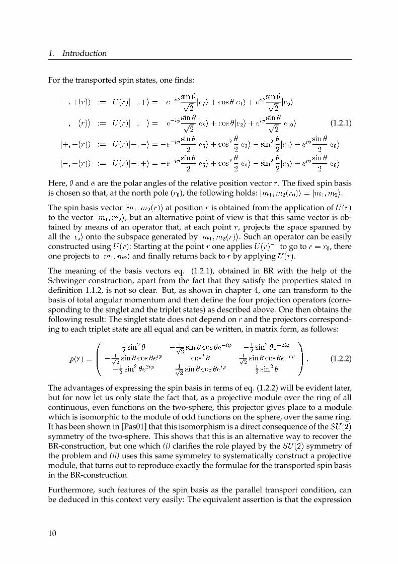
For the transported spin states, one finds:
½¾ ¿ ¾ ÀÁ Âà ÄÅ Æ ÀÁ  ½¾ ¿ ¾ à ŠÇÈÉÊË ÌÍÎ ÏÐÑ ½ÈÒ Ã ¾ ÓÔÌ Ï ½È Õà ¾ ÈÊË ÌÍÎ ÏÐÑ ½ÈÖ Ã½Ç ¿ Ç ÀÁ Âà ÄÅ Æ ÀÁ  ½Ç ¿ Çà ŠÇÈÉÊË ÌÍÎ ÏÐÑ ½È× Ã ¾ ÓÔÌ Ï ½ÈØ Ã ¾ ÈÊË ÌÍÎ ÏÐÑ ½È ÕÙ Ã (1.2.1)
½¾ ¿ Ç ÀÁ Âà ÄÅ Æ ÀÁ  ½¾ ¿ Çà ŠÇÈÉÊË ÌÍÎ ÏÑ ½ÈÚ Ã ¾ ÓÔÌØ ÏÑ ½ÈÛ Ã Ç ÌÍÎØ ÏÑ ½ÈÜ Ã ¾ ÈÊË ÌÍÎ ÏÑ ½ÈÝ Ã½Ç ¿ ¾ ÀÁ Âà ÄÅ Æ ÀÁ  ½Ç ¿ ¾ à ŠÇÈÉÊË ÌÍÎ ÏÑ ½ÈÚ Ã ¾ ÓÔÌØ ÏÑ ½ÈÜ Ã Ç ÌÍÎØ ÏÑ ½ÈÛ Ã ¾ ÈÊË ÌÍÎ ÏÑ ½ÈÝ Ã
Here, Ï and Þ are the polar angles of the relative position vector Á . The fixed spin basisis chosen so that, at the north pole (ÁÙ), the following holds:
½ß Õ ¿ ß Ø ÀÁÙ Âà Š½ß Õ ¿ ß ØÃ.The spin basis vector
½ß Õ ¿ ß Ø ÀÁ Âà at position Á is obtained from the application of Æ ÀÁ Âto the vector
½ß Õ ¿ ß Ø Ã, but an alternative point of view is that this same vector is ob-tained by means of an operator that, at each point Á , projects the space spanned byall the
½ÈÊ Ã onto the subspace generated by½ß Õ ¿ ß Ø ÀÁ ÂÃ. Such an operator can be easily
constructed using Æ ÀÁ Â: Starting at the point Á one applies Æ ÀÁ ÂÉÕto go to Á Å ÁÙ , there
one projects to½ß Õ ¿ ß Ø Ã and finally returns back to Á by applying Æ ÀÁ Â.
The meaning of the basis vectors eq. (1.2.1), obtained in BR with the help of theSchwinger construction, apart from the fact that they satisfy the properties stated indefinition 1.1.2, is not so clear. But, as shown in chapter 4, one can transform to thebasis of total angular momentum and then define the four projection operators (corre-sponding to the singlet and the triplet states) as described above. One then obtains thefollowing result: The singlet state does not depend on Á and the projectors correspond-ing to each triplet state are all equal and can be written, in matrix form, as follows:
à ÀÁ Â Åáâã
ÕØ ÌÍÎ Ø Ï Ç ÕäØ ÌÍÎ Ï ÓÔÌ ÏÈÉÊå Ç ÕØ ÌÍÎ Ø ÏÈÉØÊåÇ ÕäØ ÌÍÎ Ï ÓÔÌ ÏÈÊå ÓÔÌØ Ï ÕäØ ÌÍÎ Ï ÓÔÌ ÏÈÉÊåÇ ÕØ ÌÍÎØ ÏÈØÊå ÕäØ ÌÍÎ Ï ÓÔÌ ÏÈÊå ÕØ ÌÍÎ Ø Ï
æçè é (1.2.2)
The advantages of expressing the spin basis in terms of eq. (1.2.2) will be evident later,but for now let us only state the fact that, as a projective module over the ring of allcontinuous, even functions on the two-sphere, this projector gives place to a modulewhich is isomorphic to the module of odd functions on the sphere, over the same ring.It has been shown in [Pas01] that this isomorphism is a direct consequence of the ê Æ ÀÑÂsymmetry of the two-sphere. This shows that this is an alternative way to recover theBR-construction, but one which (i) clarifies the role played by the ê Æ ÀÑÂ symmetry ofthe problem and (ii) uses this same symmetry to systematically construct a projectivemodule, that turns out to reproduce exactly the formulae for the transported spin basisin the BR-construction.
Furthermore, such features of the spin basis as the parallel transport condition, canbe deduced in this context very easily: The equivalent assertion is that the expression
10

1.2. On the present work
ë ìë ìë vanishes or, in other words, the bundle corresponding to the projector ë is flat.Additional to the í î ïðñ symmetry, there is also an exchange symmetry, as a conse-quence of indistinguishability. In the case of two particles, this can be easily handled;but for a finite, arbitrary number of particles, the situation changes. As will be shownin this work, the approach using the language of projective modules allows for a veryclear treatment of the general case.
We finish this section with a description of the content of the present thesis.
In Chapter 2 (Quantization on multiply-connected configuration spaces), a review ofsome of the basic facts about Quantum Mechanics of spinless particles on multiply-connected configuration spaces is made, based on the standard literature on the topic.The main purpose of this chapter is to present the theoretical background which is thestarting point of the problem treated in this thesis. Although all of the results pre-sented in this chapter are well known, they are of much relevance, since they providewell-founded explanations for many of the assumptions that are made in the studyof the Spin-Statistics problem, specially the physical reasons why such mathematicalstructures as vector bundles and connections must be used.
Chapter 3 (G-spaces and projective modules) is devoted to the deduction of somemathematical results that will be needed in the following chapters. The case of a ò-free space ó (with ò a finite group) and òôbundles over it is considered. The knownequivalence of òôbundles over ó and bundles over ó õò is reformulated in a waythat allows a useful interpretation when the same problem is formulated in terms ofprojective modules. It is shown that, given a vector bundle ö over ó õò , the module ofsections ÷ ïö ñ is isomorphic to the submodule of invariant sections of the pull-back ofö . An alternative version of this result in terms of only the underlying algebras ø ïó ñand ø ïó õò ñ is worked out in last part of the chapter, where a decomposition of ø ïó ñinto ø ïó õò ñ-submodules is obtained, that allows to represent sections of bundles overó õò as functions on ó .
Chapter 4 (The spin zero case) is devoted to the discussion of two examples (using thesphere and the projective space), where the methods of chapter 3 are illustrated. Theseexamples are used in the last section of the chapter in order to discuss the case of twospin zero particles.
In Chapter 5 (Applications to the Berry-Robbins approach to Spin-Statistics), the meth-ods developed in the previous chapters are applied in an analysis of the Berry-Robbinsconstruction. This analysis leads to the conclusion that the single-valuedness condi-tion, as stated in [BR97] is inconsistent.
Chapter 6 (Further developments) contains a proposal, based on the techniques devel-oped in Chapter 3 and on the conclusions drawn from the analysis in Chapter 5, tostudy the Spin-Statistics problem.
11
2. Quantization on multiply-connected
configuration spaces
Quantum indistinguishability forces us to consider configuration spaces that have non-trivial topologies. If the states of the quantum theory are represented as functions onthese configuration spaces, the problem on quantization on multiply connected spaceimmediately arises. In the present chapter, of motivational character, we will reviewone of the possible ways in which one can implement a quantization program in suchspaces. For us, the relevance of the method reviewed in the present chapter is that itprovides a firm conceptual basis that supports the assumptions we will make in thefollowing part of the work.
2.1. Motivation
Having its origin in the fact that in Quantum Mechanics physical (pure) states are rep-resented not by vectors in Hilbert space but by rays on it, the gauge freedom of the quan-tum mechanical wave function leads very naturally to questions of a topological na-ture. Consider a wave function ù ú û ü ý defined on some classical configurationspace û. Since it is only to þù ÿ� � þ� -the probability density- that a physical meaningis attached, we are always free to modify the wave function by adding a global phasefactor, ù ÿ� � �ü ���ù ÿ� �, without changing the physical predictions. A more general kindof transformation is indeed allowed: a local one, of the form ù ÿ� � �ü ��� � ù ÿ� �.The question, as to what extent is it possible to make a globally well defined choice ofphase, i.e., of a function û ü ý ú � �ü ��� � , was already considered by Pauli [Pau39].He noticed that this is possible whenever û is simply connected.
Phase ambiguities do also show up in the path integral formulation of Quantum Me-chanics [FH65], where they arise as a consequence of the gauge freedom of the La-grangian. Consider a classical system defined on a configuration space û and de-scribed by a Lagrangian � ÿ� � � � � �. A gauge transformation of the Lagrangian, of theform � ÿ� � � � � � �ü �� ÿ� � � � � � � � ÿ� � � � � � � ��� � ÿ� � � �12
2.1. Motivation
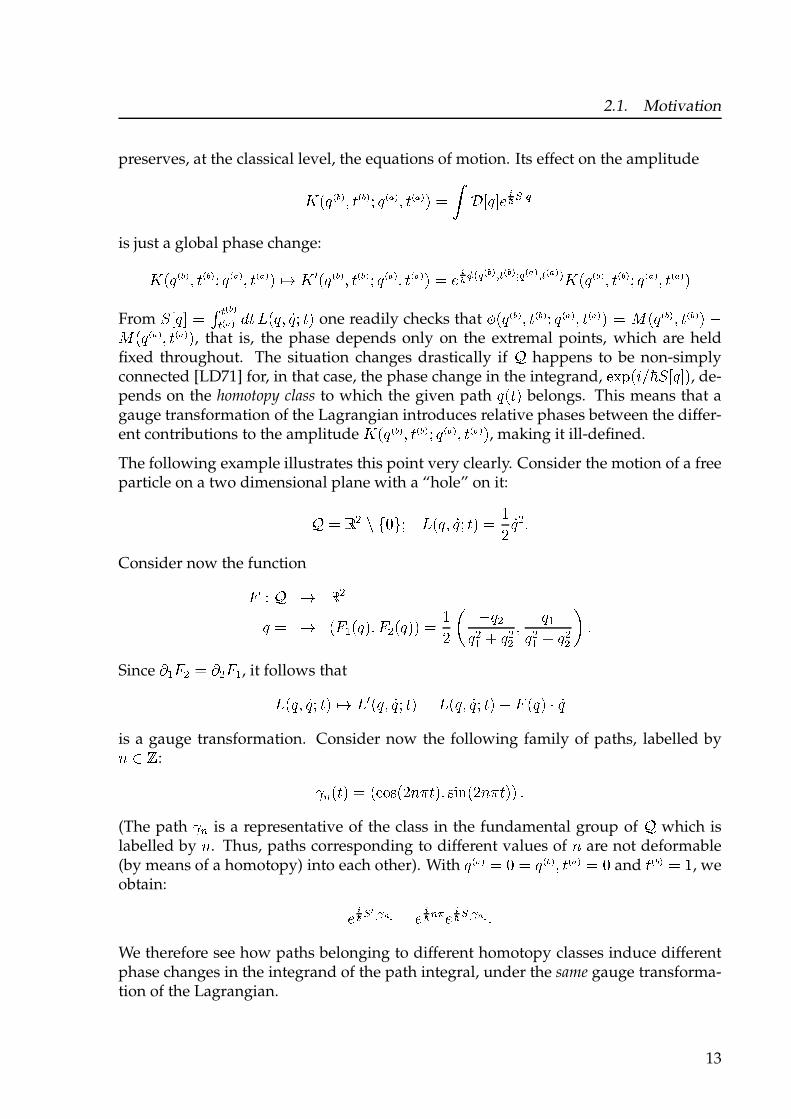
preserves, at the classical level, the equations of motion. Its effect on the amplitude� �� ��� � � ��� � � ��� � � �� � � ! " #� $% &' ( )*+is just a global phase change:� �� ��� � � ��� � � ��� � � �� � � ,- � . �� ��� � � ��� � � ��� � � �� � � % &' / 0* ��� 12 ��� 3* ��� 12 �� � 4� �� ��� � � ��� � � �� � � � ��� �From 5 #� $ 6 2 ���2 �� � 7� 8 �� � 9� � � � one readily checks that : �� ��� � � ��� � � �� � � � ��� � ; �� ��� � � ��� � <; �� �� � � � �� � �
, that is, the phase depends only on the extremal points, which are heldfixed throughout. The situation changes drastically if = happens to be non-simplyconnected [LD71] for, in that case, the phase change in the integrand, >?@ �ABC5 #� $�, de-pends on the homotopy class to which the given path
� �� �belongs. This means that a
gauge transformation of the Lagrangian introduces relative phases between the differ-ent contributions to the amplitude
� �� ��� � � ��� � � ��� � � �� � �, making it ill-defined.
The following example illustrates this point very clearly. Consider the motion of a freeparticle on a two dimensional plane with a “hole” on it:= D E F GHI� 8 �� � 9� � � � JK 9� E LConsider now the functionM N = - D E� ,- �M O �� �� ME �� �� JK P <�E� EO Q � EE � � O� EO Q � EE R LSince S OME SEM O, it follows that8 �� � 9� � � � ,- 8. �� � 9� � � � 8 �� � 9� � � � Q M �� � T 9�is a gauge transformation. Consider now the following family of paths, labelled byU V W : XY �� � �Z[\ �KU] ��� \^_ �KU] ��� L(The path
XYis a representative of the class in the fundamental group of = which is
labelled by U. Thus, paths corresponding to different values of U are not deformable(by means of a homotopy) into each other). With
� �� � H � ��� � � ��� Hand
� ��� J, weobtain: % &' ( ` )ab + % &' Yc % &' ( )ab + LWe therefore see how paths belonging to different homotopy classes induce differentphase changes in the integrand of the path integral, under the same gauge transforma-tion of the Lagrangian.
13

2. Quantization on multiply-connected configuration spaces
This new feature of the path integral for non-simply connected spaces was first pointedout by Schulman[Sch68]. A more general treatment was later on presented by Laidlawand DeWitt[LD71], where they showed how the non-trivial topology of the configura-tion space leads to different, inequivalent quantizations of the same classical system.
Very roughly, the idea of their proof is as follows. Since, as we have just seen, pathsbelonging to different homotopy classes cannot be included in the path integral at thesame time, only partial amplitudes d e containing sums over paths belonging to thesame homotopy class (labeled by the element f of the fundamental group g h ijkl) canbe consistently defined. In order to include all paths one then adds the different am-plitudes d e , but there is no a priori reason why this sum might not be a weighted sum,of the form d m neop q rst u if kd e v (2.1.1)
The form of the weight factors u if k is determined from certain -rather technical- prop-erties that the partial propagators can be shown to have and that we will not discusshere (for details, see [LD71] and [Sch68]).
However, it is important to point out that physical considerations play an essential rolein the determination of the weight factors. For example, the consistency requirementwd ix y z{ | } y z~ k w m ����� d ix y z{ | � y z� kd i� y z� | } y z~ k�� ���� yimposed on the total propagator, has a clear physical meaning and is used in thederivation of the final result, which can be stated as follows:
2.1.1. Theorem (cf.[LD71]). The weight factors u if k in eq. (2.1.1) must form a one-dimensional unitary representation of the fundamental group.
An immediate consequence of this result is that there are as a many possible quantiza-tions of the classical system described by � on j, as there are characters of g h ijk. Al-though not clear at this point, these quantizations are inequivalent for different choicesof the character u.
A particularly relevant application of this theorem is obtained for a system of identicalparticles: Consider � identical particles moving in three dimensional Euclidean space.If the configuration space is, as described in the first chapter, taken to bej m i� � � � � � � � � � � k��� y�
Here we are considering paths beginning at some point � and ending at some point � in �. In orderto assign an element of � � ��� to each such path, an arbitrary point �� � � is chosen, as well as anassignment of paths (“homotopy mesh”[LD71]) � �� � going from � to �� , for every � in �. In thisway, a path � going from � to �, can be assigned the map � ���� � �� ���, which belongs to a givenelement of � � ��� �� �
14

2.2. Canonical Quantization from Group Actions
where � denotes the permutation group, then there are exactly two characters, cor-responding to the completely symmetric/antisymmetric one dimensional representa-tions, and hence to Bose/Fermi statistics.
In spite of its applicability being restricted to systems of spinless particles, this is indeeda very strong result: It says that, if we take indistinguishability properly into account,there is no need for a symmetrization postulate since, in three dimensions, the twophysically observed statistics, fermionic or bosonic, are the only allowed ones.
At the beginning of this section, we started our discussion with questions related to theproblem of fixing the phase of the wave function globally. This is a question that canbe more clearly formulated using the notion of fiber bundle. Since the phase is (at leastlocally) a ¡ ¢£¤-valued function, one can consider it as a section of a principal ¡ ¢£¤-bundle. Equivalently, one can consider a line bundle associated to this ¡ ¢£¤-bundle,and take the wave function to be a cross-section of this line bundle. In this context,different quantizations arise, among other things, from the choice of the bundle wherethe wave function is defined. The relation of a fiber bundle approach to the Feynmanfunctional one we have just discussed is not clear at all, but we shall see, in the nextsections, how the conclusion of theorem 2.1.1 might be obtained from a quantizationscheme that is based on the action of a so-called canonical group on the classical phasespace. Within this approach, the quantum theory is obtained from the representationtheory of the canonical group, and this in turn leads naturally to a fiber bundle formu-lation.
The Feynman functional approach has the advantage of providing a very clear pic-ture of why the topology of the configuration space of a classical system might beseen reflected in the corresponding quantized theory: In the sum over “histories” pre-scription, all paths between two given points give contributions to the probability am-plitude, so that they provide information on the global structure of the configurationspace. On the other hand, the approach presented in the next sections deals with thedifficulties that arise when one attempts to apply a canonical quantization prescriptionto a system with a configuration space that has a non-trivial topology (in the sense ofbeing, e.g., multiply connected). Then, the need to use fiber bundles and representa-tion theory arises in a very natural way, providing a justification, from the point ofview of physics, of the setting on which the present work is based.
2.2. Canonical Quantization from Group Actions
2.2.1. Preliminary remarks
We have discussed the effects that the global structure of a classical configuration spacemay have on the quantum theory obtained from a classical Lagrangian by means of
15
2. Quantization on multiply-connected configuration spaces
Feynman’s path integral formulation. As already pointed out, this approach is partic-ularly useful in order to get a “feeling” of why -if at all- the topology of the configura-tion space should play a role in the quantization of the system. For us, the interest inthese kind of “topological effects” lies in the fact that, as illustrated in the previous sec-tion, for a system of ¥ identical spinless particles, the Fermi-Bose alternative followsdirectly as a restriction imposed by the topology of the configuration space. The topo-logical non-triviality of this space, expressed by the fact that its fundamental group isisomorphic to the permutation group of ¥ elements, determines the allowed statisticswithout the need to consider a symmetrization postulate.
Whether the fact that the topology of this configuration space is not trivial might beused to derive the Spin-Statistics relation, has been (and still is) a source of contro-versy. Many authors are of the opinion that there is no way at all of relating spinwith statistics, unless one goes over to relativistic quantum field theory (see, for ex-ample, [Wig00]). Perhaps this is true: Much effort has been put in the search for anon-relativistic proof and, as time went by, it became clearer that there is some essen-tial physical assumption that is still missing. This could be, for example, some kind ofcondition that must be imposed in the non-relativistic theory, arising as a “shadow”or “remanent” of properties inherent to the relativistic quantum theory. If such a con-dition could be found and consistently incorporated into a configuration space (topo-logical) approach in order to obtain a non relativistic version of the Spin-Statistics The-orem, we could certainly learn more about the relativistic case. Another interestingpossibility is that topological spaces such as the one defined in eq.(1.1.2) or gener-alizations thereof might appear in a natural way in a Quantum Field Theory. Ideasalong this line have been put forward by Tscheuschner [Tsc89] and Balachandran et.al. [BDG¦90, BDG¦93]. A full mathematical understanding of the very interesting(but to a great extent heuristic) ideas presented by these authors would justify by itselffurther studies within a configuration space approach.
In spite of all this, we want to stick to the point of view that the configuration spacedefined in eq.(1.1.2) does have something to do with the relation between spin andstatistics. The reasons that -to our opinion- justify our assuming this point of view, arethe following:§ Relevance of the structure of classical theories for the formulation and under-
standing of quantum ones:
Although nowadays there exist approaches to Quantum Theory which are notbased on a quantization of some underlying classical theory, both the historicaland conceptual relevance of the structure of the classical mechanics (of particlesand fields) for the formulation of Quantum Theory cannot be overseen. Funda-mental structures and concepts, like the symplectic structure of phase space, thePoisson bracket algebra or Noether’s theorem have played (and still play) a pri-mordial role as guidelines in the search for a Quantum Theory in many branchesof physics. Additionally, there are many situations where all one has to start withis a classical theory that is believed to be a limit of some, more fundamental,
16
2.2. Canonical Quantization from Group Actions
quantum theory. Needless to say, two prominent examples of this situation arethe relations between Maxwell’s theory of electromagnetism and Quantum Elec-trodynamics on one hand and between General Relativity and its sought-afterquantum version, on the other. In the same way, one expects some kind of re-lation between the classical mechanics of a system of identical particles and itsquantum version.¨ The notion of space in quantum mechanics: In most physical theories, space-time plays a passive role, in the sense that it is the “stage” where all physicalphenomena take place. The space-time of every theory has a symmetry group.The dynamical rules of a theory must be formulated in such a way that theyare compatible with the symmetry group, but space-time itself does not play adynamical role©. In this sense, one could say that space-time is “what remainswhen one takes away all particles, fields, etc..”. From this point of view, in quan-tum mechanics, when one considers one particle, space is what remains afterremoving this particle: ª « . But, when considering two particles, the structure ofthe “space” that remains after taking away the particles should be expected tobe very different from the one corresponding to a single particle. This becauseof indistinguishability. The configuration space of eq.(1.1.2) may be seen as themathematical expression of this idea.¨ Gibbs’ paradox: This was one of the main motivations for Leinaas and Myr-heim [LM77] in order to study the configuration space eq.(1.1.2). Gibbs’ paradoxshows that, even if we remain at a classical level ¬, when asking questions about themicroscopic properties of a system of identical particles, the configuration spaceeq.(1.1.2) must be used, in order to avoid inconsistencies.¨ Relevance of the Spin-Statistics relation in the non-relativistic context: Aspointed out in the introduction, the observed relation between Spin and Statisticshas many consequences and is crucial for the understanding of many physicalphenomena that take place in a quantum, but non-relativistic, domain. Non-relativistic Quantum Mechanics is a theory that can be consistently formulatedwithout the need of concepts of relativity. On the other hand, the only (generallyaccepted) proofs of the Spin-Statistics Theorem make use of Poincare invariancein an essential way. There remains the question of why must one make use innon-relativistic Quantum Mechanics, a theory standing on its own, of a resultthat has been proved somewhere else?¨ Relation to relativistic QFT: Even if at the end it turns out that there is no wayof finding a non-relativistic proof of the Spin-Statistics Theorem, the techniquesdeveloped in such a search could eventually be used to have a different look atthe problem such as an interpretation of the relativistic, analytical proofs in geo-metric/topological terms. It is in part because of this possibility that the config-
General Relativity being, of course, an exception.®With this we mean: Even if the Maxwell-Boltzmann distribution is being used, see [LM77].
17
2. Quantization on multiply-connected configuration spaces
uration approach to indistinguishability proposed in the present work, which isof a geometric/topological nature, has been also formulated in a more algebraiclanguage, one that lies closer to the one of Quantum Field Theory.
Having stated the reasons why we are interested in studying the effects that a configu-ration space as eq.(1.1.2) might have on the Quantum Theory, we now turn to the cen-tral theme of this chapter: Quantization on a multiply-connected configuration space.Assume we are given a classical configuration space ¯ with a non-trivial global struc-ture (the specific example of interest for us is that of ¯ being multiply-connected).We then try to construct a quantum theory, having as starting point a classical the-ory based on ¯. When such an attempt is made, one encounters very soon problemswith the application of the usual “quantization rules” that work so well in the case of¯ ° ± ² . The aim of the brief account to quantization that we present in this chap-ter is to provide well-founded arguments in favor of the idea that, when dealing witha globally-structured configuration space ¯, some of the usual assumptions that aremade in the case of ± ² , have to be reconsidered, this leading to the need to considera more general setting for the quantum theory. This more general setting will be thestarting point for our considerations about the Spin-Statistics relation.
Among the assumptions we alluded to above, we have:
(1.) The Canonical Commutation Relations (CCR),³µ ¶ · ´¹ º ° »¼½ ¶¹ · ³µ ¶ · µ ¹ º ° ¾ ° ¿ ´¶ · ´¹ À · (2.2.1)
hold.
(2.) A (Pure) state Á is a function defined on ¯ and taking values on a complex vectorspace: Á Â ¯ Ã Ä Å Æ
The fact that the CCR cannot hold unrestricted for any configuration space is some-thing plausible because, whereas in the case of ¯ ° ± ² the position and momentumoperators are the quantized versions of the global coordinates ǵ È · Æ Æ Æ · µ ² É ¸ È · Æ Æ Æ · ¸ ² Ê(defined for the phase space Ë Ì± ² ), in a general configuration space the use of morethan one local coordinate chart might be necessary, and then the need to define globalposition and momentum operators, or suitable analogs of them, arises. The kind ofpermutation relations that these new operators obey will then clearly depend on theglobal structure of ¯. The “breakdown” of the usual CCR has consequences in theway that pure states are realized. This is so because the space where these states “live”is a representation space of an abstract algebra whose generators obey the CCR. Theposition and momentum operators can then be seen as the operators representing thegenerators of this algebra. But if the algebra admits different, inequivalent represen-tations, it could well happen that the representation space takes a form different from
18

2.2. Canonical Quantization from Group Actions
the usual one (a space of complex functions defined on Í). That this is not the case forthe familiar example of quantum theory on Î Ï is a direct consequence of the Stone-vonNeumann theorem.
In some cases, the representation space where the state vectors are defined takes theform of a space of sections of some vector bundle over Í. For a given classical the-ory, different, inequivalent quantizations may be possible, and this could be reflectedin the fact that the corresponding state functions will be sections defined on topologi-cally inequivalent vector bundles over Í. It could also happen that two (inequivalent)representations take place on the space of sections of the same bundle, but that there issome parameter that singles out the representations as being inequivalent. One wayin which this may happen is in the choice of a certain flat connection that makes itsappearance in the process of quantization.
The remarks above will be illustrated in the remaining sections of this chapter, follow-ing an approach to quantization where the relevance of group actions and its relationto topological effects in quantum theory are emphasized. The basic reference we havefollowed for this topic is the article by C.J. Isham, from the Les Houches session of1983 [Ish84]. Other useful references are [Mor92, HMS89]. There are, of course, manyapproaches to quantization, from quite different points of view. One of them is, forexample, geometric quantization [Sou69, Woo80]. More recent approaches include, forexample, deformation quantization [BFFÐ78, Fed94]. But, for our purposes, the veryreadable account of Isham will suffice.
2.2.2. From CCR to group actions and back
A very nice way to see that the usual CCR cannot hold for every configuration space, isprovided by quantum theory based on the positive real line, Î Ð . Assume that the usualdefinition for the position and momentum operators can also be used in this case:Ñ ÒÓÔ ÕÑÓ Õ Ö ÓÔ ÑÓ Õ (2.2.2)Ñ Ò× Ô ÕÑÓ Õ Ö ØÙÚ ÛÛÓ Ô ÑÓ ÕÜLet us assume that we can take as Hilbert space Ý Ö Þß ÑÎ Ð à ÛÓ Õ. Now, assume for amoment that the operator defined by eq. (2.2.2) is self-adjoint (it is not). If this werethe case, then we could affirm that this operator is the infinitesimal generator of trans-lations, i.e., with á Ñâ Õ ãÖ äåæç èé we would obtain a unitary operator in Ý whose actionon wave functions would be Ñá Ñâ ÕÔ ÕÑÓ Õ Ö Ô ÑÓ Ø Úâ ÕÜ (2.2.3)
But clearly this cannot be possible, since we could always chooseâ
in such a waythat the support of á Ñâ ÕÔ ends up lying outside Î Ð . Therefore, the usual definitionof position and momentum operators does not work for this space. If the basic CCR
19
2. Quantization on multiply-connected configuration spaces
cannot be imposed on this configuration space, what kind of operators could then bedefined on it, and in that case, what kind of commutation relations would they obey?In order to answer this questions, it is necessary to answer first another one: What isthe “origin” of the usual CCR in the familiar case of quantum theory on ê (or ê ë )? Thisquestion is to be interpreted in the following sense. As the above example suggests,the fact that the CCR cannot hold in a given configuration space ì, has somethingto do with the structure of ì. Note that the main difference between ê and ê í isthat, whereas the former is a vector space, the latter is not. So, the question about the“origin” of the CCR on ê could be reformulated by asking: What are the properties ofê that allow the CCR to hold?
One way to answer the question posed above is by considering the exponentiated(Weyl) form of the CCR. Defining the unitary operatorsî ïð ñ òó ôõö÷ øù ú û ïüñ òó ôõöý øþ ú (2.2.4)
acting on ÿ � ïê ú �� ñ, we obtain the following relations:î ïð � ñî ïð� ñ ó î ïð � � ð� ñ úû ïü � ñû ïü� ñ ó û ïü � � ü� ñú (2.2.5)î ïð ñû ïüñ ó ôö�÷ý û ïü ñî ïð ñ �These relations follow readily from the action of
î ïð ñ andû ïüñ on wave functions:ïî ïð ñ� ñï� ñ ó � ï� � ð ñú (2.2.6)ïû ïüñ� ñï� ñ ó ôõöýþ� ï� ñ �
The commutation relations eq.(2.2.5) suggest that we are dealing with a representationof some group. This is in fact true, and the underlying group is called the HeisenbergGroup. It can be defined not only for ê but also for ê ë . As a set, it is given by ê ë ê ë ê ,with the group lawïð � ú ü � � � �ñ ïð� ú ü� � �� ñ òó ïð � � ð � ú ü � � ü� � � � � �� � �� ïü � ð� � ü� ð � ññ � (2.2.7)
Fromïð ú � � � ñõ � ó ï�ð ú � � � ñ and
ï� ú ü � � ñõ � ó ï� ú �ü � � ñ, one checks:ïð ú � � � ñ ï� ú ü � � ñ ïð ú � � � ñõ � ï� ú ü � � ñõ � óó ïð ú � � � ñ ï� ú ü � � ñ ï�ð ú � � � ñ ï� ú �ü � � ñó ïð ú ü � � �� ðüñ ï�ð ú �ü � � �� ðüñó ï� ú � � �ðüñ �Thus we see that, if we define a representation � of the Heisenberg group on the spaceÿ � ïê ú �� ñ by
� ïïð ú � � � ññ òó î ïð ñú� ïï� ú ü � � ññ òó û ïüñú (2.2.8)� ïï� ú � � � ññ òó ôö�� id ú
20
2.2. Canonical Quantization from Group Actions
we can get the commutation relations eq. (2.2.5) from this representation of the Heisen-berg group. In order to see how the Heisenberg group is related to the symplecticstructure of the phase space � �� � , it is convenient to consider its action (through theoperators � and � ) on the position and momentum operators:
� �� � �� � �� ��� �� ! "� # (2.2.9)� �$� �% � �$��� �% & "$ 'These relations suggest that we consider the following transformation:
�� � ( � � � ( � �� � ) � �� � (2.2.10)��� # $ �# �* # % �� +) �* ! � #% & $�'If we see � � (� � as an additive group, then eq.(2.2.10) gives place to a group action on� �� � . Although not clear at this point, starting from this group action one can arrivein a quite systematic way to the conclusion that the Heisenberg group provides thesolution to the quantization problem on � � . For the moment, let us just mention thatthe action eq.(2.2.10) is symplectic, transitive and effective.
Summing up, what we have done until now is to realize that there is a group acting onthe classical phase space, that this group is in a certain form related to the Heisenberggroup and that the CCR (in their Weyl form) can be obtained from a representation ofthe Heisenberg group on ,- �� # .� �.The link between the classical and the quantum theory on /� can be directly estab-lished at the infinitesimal level, by considering Dirac’s quantization conditions, which
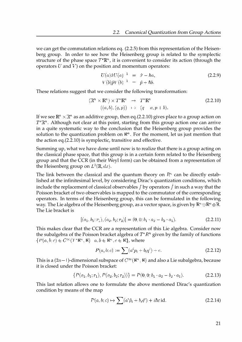
include the replacement of classical observables 0 by operators �0 in such a way that thePoisson bracket of two observables is mapped to the commutator of the correspondingoperators. In terms of the Heisenberg group, this can be formulated in the followingway. The Lie algebra of the Heisenberg group, as a vector space, is given by � � 1� � 1� .The Lie bracket is 2
�� � # $ � 3 4 � �# ��- # $- 3 4- �5 �6 # 6 3 $ � 7 �- ! $- 7 � � �' (2.2.11)
This makes clear that the CCR are a representation of this Lie algebra. Consider nowthe subalgebra of the Poisson bracket algebra of � �/� given by the family of functions89 �� # $ 3 : � ; < = �� �� � # � � > � # $ ; � � # : ; � ?, where9 �� # $ 3 :� @ A ��B% B & $B * B � & : ' (2.2.12)
This is a (CD & E)-dimensional subspace of < = �� � # � � and also a Lie subalgebra, becauseit is closed under the Poisson bracket:89 �� � # $ � 3 4 � � # 9 ��- # $- 3 4- ��? 9 �6 # 6 3 $ � 7 �- ! $- 7 � � �' (2.2.13)
This last relation allows one to formulate the above mentioned Dirac’s quantizationcondition by means of the map9 �� # $ 3 :� +) A ��B �% B & $B �* B � & F": id ' (2.2.14)
21

2. Quantization on multiply-connected configuration spaces
Note that from eqns. (2.2.11) and (2.2.13) it is clear that this map takes the Poissonbracket GH I J K L M N OIL to P QH I J QK L R N STO IL .This seems to make the consideration of the symplectic action of the additive groupU V W U V
on X YU V unnecessary. But, as explained below, in a generic case, the existenceof a group action on phase space, fulfilling certain conditions, will be the starting pointfor the construction of the corresponding quantum theory.
With these remarks about the case of X YU V in mind, let us very briefly present themain ideas about the quantization scheme presented in [Ish84]. The starting point is aclassical phase space Z , i.e., a symplectic manifold. In most examples this phase spaceis the one associated to a configuration space [: Z N X Y [.
There are two main stages into which the scheme can be divided.
(1) Find a finite dimensional Lie Group (\ ) which is related (in a way to be specified)to a group (] ) of symplectic transformations of the phase space Z and such that:
(i) Its Lie algebra ^ _\ ` is a subalgebra of the Poisson bracket algebra_a b _Z J U `J G J M`.(ii) ^ _\ ` is big enough to generate as many (classical) observables as possible.
(2) Study the unitary, irreducible representations of \ . The self-adjoint generatorscan be considered as the quantized versions of the corresponding classical ob-servables.
As observed before, in the case of [ N U V, the relation between the groups \ (Heisen-
berg group) and ] (the additive groupU V W U V
) is not clear a priori. This is due to theexistence of a certain obstruction (for details, see further below) that arises when oneattempts to assign a classical observable (i.e. a function in _a b _Z J U `) to each elementof ^ _] `` in such a way that the Lie bracket is preserved.
One of the reasons why the scheme consists in starting with a group that acts on Z andthen in trying to associate its Lie algebra with functions on Z is that if this associationcan be constructed in the form of a Lie algebra isomorphismc d ^ _] ` ef a b _Z J U `J (2.2.15)
one can define a quantization map by fixing a representation g of the group and as-signing to each function lying in the image of
cthe self-adjoint generator obtained
from g by means ofc hi
.
Whereas the existence of a mapc
having the desired properties is not something ob-vious, in the opposite direction, there is a natural way to implement such a procedure.Indeed, given a (finite dimensional) Lie subalgebra j of a b _Z J U `, consider the Hamil-tonian vector field that a function k l j generates: mn . This vector field gives place toa one-parameter subgroup, acting by symplectic transformations. If these vector fields
22

2.2. Canonical Quantization from Group Actions
are complete, their one-parameter subgroups will generate a group o of symplectictransformations and, if the mapping sending p into the set of Hamiltonian vector fieldsis injective, we obtain a Lie algebra isomorphism p qr s to u.Thus, the idea is, starting with a group o of symplectic transformations, to find a kindof “inverse” to the map
v w x y tz { | u } Ham VFtz u (2.2.16)~ �} ���and then to pre-compose it with a map � w s to u } Ham VFtz u. The map � is naturallyinduced by the o -action on
z, but in order that its image be restricted to only the set
of Hamiltonian vector fields and that it be an isomorphism, some conditions must beimposed.
The situation can be summarized by saying that one looks for a map � that makes thefollowing diagram commute:� | x y tz { | u � HamVFtz u �
s to u��
The kernel of v consists of the set of constant functions on phase space, so the firstrow represents a short exact sequence. There are two main problems in relation to thisdiagram. The first one has to do with the conditions that should be imposed on theaction in order that the map � produces globally Hamiltonian vector fields. The secondone comes from the requirement that the map � respects the Lie algebra structure. Inorder to understand this in some detail, let us consider, point by point, some of themore relevant features.� The map � :
Given a symplectic action of a Lie group on phase space, o �z } z, one can construct
a map � w s to u } VFtz u as follows. Given � � s to u, consider the map sending� � | to ��� � o . Then, using the action, one can define a one-parameter subgroup ofsymplectic transformations on
z, given by��� t� u wr ���� � � t� � z u�
From this we obtain a vector field � � , defined through its action on functions:
� �� t~ u wr ��� ~ t��� t� uu ���� � (2.2.17)
From this definition, it follows that the map � w � �} �� is a Lie algebra homomor-phism. It is clear that
�� is the local flow of � � . But��� , being a symplectic transforma-
tion, preserves the symplectic form (� ), i.e.���� � r � . This, together with the relation
23

2. Quantization on multiply-connected configuration spaces
��� � ¡� ¢£ ¤ ¥ � ¡� ¢¦§¨ £ ¤, implies that the Lie derivative ¦§¨ £ vanishes. This is a nec-essary condition in order that © be the Hamiltonian vector field of some function onphase space. But it is not sufficient. To see this, notice that from ¦§¨ ¥ ª§¨ «¬ ¬«ª§ ¨ and¬£ ¥ ®, it follows that ª§ ¨ £ is a closed one-form. But the requirement that © ¥ ¯° forsome function ± is equivalent to the requirement that ª§ ¨ £ ¥ ¬± . We thus arrive at theconclusion that a sufficient condition in order that the image of the map © lies entirelyin the set of Hamiltonian vector fields, Ham VF¢² ¤, is that every closed one-form on²
be also exact. In other words, we must require that the first cohomology group of²
vanishes. This imposes a restriction of a topological nature on the phase spaces²
thatcan be quantized using the present approach. Finally, let us mention that a sufficientcondition for the map © to be injective is that the action be effective. (A less restrictivecondition can be imposed, allowing one to replace the group ³ by a covering of it, see[Ish84]).´ The map µ and the obstruction cocycle:
If the ³ -action is effective, and if the first cohomology group of the phase space van-ishes, we obtain an isomorphism © from ¶ ¢³ ¤ into the set of Hamiltonian vector fields.But in order to be able to assign an observable to each element of ¶ ¢³ ¤, we need to finda suitable map µ · ¶ ¢³ ¤ ¸ ¹ º ¢² ¤. As indicated in the diagram above, the idea is thatthe diagram commutes, that is for » ¼ ¶ ¢³ ¤ we want to have (µ ½ µ ¢» ¤):
© ¥ ¾¯¿ ¨ À (2.2.18)
This is a natural requirement, since, as we have observed, the map Á assigns a Hamil-tonian vector field to every function on phase space, in a natural way. Up to the iso-morphism © , we are now looking for an assignment in the opposite direction, and it isnatural to expect that, if © ¢» ¤ ¥ Á ¢± ¤, then µ ¢» ¤ ¥ ± (at least up to a constant, sinceÂÃÄ Á ¥ Å ). The map µ should also be a Lie algebra isomorphism. From the requirementeq.(2.2.18) and the fact that © is a Lie algebra homomorphism, we obtain:¯¿ ƨ ÇÈ É ¥ ¯Ê¿ ¨ Ë¿ È Ì À (2.2.19)
But, sinceÂÃÄ Á ¥ Å , the only thing we can conclude is thatÍ ¢» Î Ï ¤ ·¥ е Î µ Ñ Ò ¾ µ Ó ËÑ Ô (2.2.20)
is a constant. There is some freedom in the choice of the map µ : If µ satisfieseq.(2.2.18), then the map µ Õ, defined by
µ Õ ·¥ µ ¬ ¢» ¤Î (2.2.21)
where ¬ belongs to the dual of ¶ ¢³ ¤, is also linear and satisfies eq.(2.2.18). The problemis then reduced to find a suitable ¬ ¼ ¶ ¢³ ¤¡ in such a way that the constants Í ¢» Î Ï ¤ ineq.(2.2.20) vanish for all » Î Ï .
Eq.(2.2.20) defines a real-valued 2-cocycle, that is, a map Í · ¶ ¢³ ¤ Ö¶ ¢³ ¤ ¸ Å satisfyingÍ ¢» Î Ï ¤ ¥ ¾Í ¢Ï Î » ¤Í ¢» Î ×Ï Î ¹ ؤ Í ¢Ï Î ×¹ Î » ؤ Í ¢¹ Î ×» Î Ï Ø¤ ¥ ® À24
2.2. Canonical Quantization from Group Actions
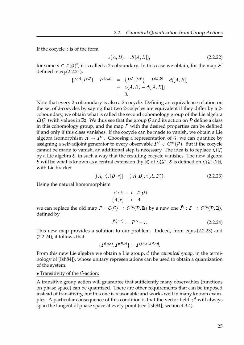
If the cocycle Ù is of the form Ù ÚÛ Ü Ý Þ ß à ÚáÛ Ü Ý âÞÜ (2.2.22)
for someà ã ä Úå Þæ, it is called a 2-coboundary. In this case we obtain, for the map ç è
defined in eq.(2.2.21),éç èê Ü ç èë ì í ç è îê ïë ð ß éç ê Ü ç ë ì í ç îê ïë ð í à ÚáÛ Ü Ý âÞß Ù ÚÛ Ü Ý Þ í à ÚáÛ Ü Ý âÞß ñ òNote that every 2-coboundary is also a 2-cocycle. Defining an equivalence relation onthe set of 2-cocycles by saying that two 2-cocycles are equivalent if they differ by a 2-coboundary, we obtain what is called the second cohomology group of the Lie algebraä Úå Þ (with values in ó ). We thus see that the group å and its action on ô define a classin this cohomology group, and the map ç with the desired properties can be definedif and only if this class vanishes. If the cocycle can be made to vanish, we obtain a Liealgebra isomorphism
Û õö ç ê . Choosing a representation of å , we can quantize byassigning a self-adjoint generator to every observable ç ê ã ÷ ø Úô Þ. But if the cocyclecannot be made to vanish, an additional step is necessary. The idea is to replace
ä Úå Þby a Lie algebra ù , in such a way that the resulting cocycle vanishes. The new algebraù will be what is known as a central extension (by ó ) of
ä Úå Þ. ù is defined onä Úå Þ ú ó ,
with Lie bracket áÚÛ Ü û ÞÜ ÚÝ Ü üÞâ ß ÚáÛ Ü Ý â Ü Ù ÚÛ Ü Ý ÞÞò (2.2.23)
Using the natural homomorphism ý þ ù ö ä Úå ÞÚÛ Ü û Þ õö Û Üwe can replace the old map ç þ ä Úå Þ ö ÷ ø Úô Ü ó Þ by a new one ÿç þ ù ö ÷ ø Úô Ü ó Þ,defined by ÿç �ê ï� � þß ç ê � û ò
(2.2.24)
This new map provides a solution to our problem. Indeed, from eqns.(2.2.23) and(2.2.24), it follows that é ÿç �ê ï� � Ü ÿç �ë ï��ì ß ÿç î�ê ï� � ï�ë ï��ð òFrom this new Lie algebra we obtain a Lie group, � (the canonical group, in the termi-nology of [Ish84]), whose unitary representations can be used to obtain a quantizationof the system.� Transitivity of the å -action:
A transitive group action will guarantee that sufficiently many observables (functionson phase space) can be quantized. There are other requirements that can be imposedinstead of transitivity, but this one is reasonable and works well in many known exam-ples. A particular consequence of this condition is that the vector field � ê will alwaysspan the tangent of phase space at every point (see [Ish84], section 4.3.4).
25

2. Quantization on multiply-connected configuration spaces
2.2.3. Representations of the canonical group
When the phase space � is the cotangent bundle of a configuration space , thereare two natural classes of transformations that one can consider. The first class is theone induced by the diffeomorphism group of on � : If � Diff, then using thepull-back of � we obtain a transformation (� �� and � �� ) defined by:
��� � � � �� � �� � ��� �� �� � � (2.2.25)
The map � �� �� � is, in particular, a symplectic transformation on � . Thus, sub-groups of Diff are possible candidates for the canonical group. The difficulty is thatthis action is not transitive. For this reason, this class of transformations has to becomplemented by a second one. The second class of transformations is induced byfunctions on , as follows. Given � � � �� � we can use its exterior differential togenerate “translations” along the fibers of � , mapping � �� to � ! �"� � �� . Itturns out that this transformation is also a symplectic transformation. Notice that since� acts only through its differential
"�, it is really the quotient group � � �� � #� thatis being considered: Two functions differing by a constant produce the same transfor-mation.
We thus have two different group actions on � :
Diff $ � � � �� � � �� �%&� �
and
� � �� � #� $ � � � �' � � �� � ! �"' � �� �� �
It is not difficult to see that the set of Diff-induced transformations plus the set of the� � �� � -induced ones is transitive on � . It is therefore natural to try to expressthem as the action of a single group on � , whose underlying set is � � �� � #� $Diff. The group law is determined by the requirement that it must be compatible withthe action. Denoting with ( the action, we have (for ' � � �� � #� , � Diff and � �� ):
( �) *� � �� +� �%&� �� ! �"' � �� � �From the requirement (,- .(, / 0� (,-, / we obtain:
( �)- *� - �.( �) / *�- � �� �� ( �)- *�- � ��%&�& �� ! �"' & � / �� � � �%&�1 ��%&�& �� ! �"' � / �� � ! �"'1 �-.� / �� �� ���1.� & %& � �� ! " ��%&�1 ' & ! '1 �- .� / �� �� ( ��- .� / *) /.�2/- 3)- � �� �
26

2.2. Canonical Quantization from Group Actions
Thus, the structure obtained is that of the semi-direct product 4 5 6789: ; Diff7. Thisgroup has several interesting properties. Among them, it fulfills all the requirementsneeded to implement the quantization procedure (for details, the reader is referred to[Ish84]). In particular, the map < that it induces produces Hamiltonian vector fields.For the class of examples where this group can be used, the quantization problemreduces to finding a suitable finite dimensional subspace = of 4 5 6789: and a finitedimensional subgroup > of Diff7 and then to study the representations of the group= ; > .
The fact that for the scheme we have been discussing the basic structure is that of agroup acting by symplectic transformations on phase space, provides the justificationfor a re-examination of the basic assumption, stated in the last section, that pure statesare always expressible as functions. Indeed, since the quantum theory is obtained fromthe unitary representations of the canonical group, there is no a priori reason to discardone representation in favor of another one. Inequivalent representations might be as-sociated with the same classical system, leading to different quantizations of it. Someof these representations will lead to states that are expressible in the form of functions,but there might be other representations for which the representation space is, for in-stance, some space of cross-sections of a vector bundle over the configuration space.These kind of representation arise naturally when one has a group > acting on a space?
. If, for example, @ A ? B Cbelong to some set of functions on
?, the >-action
induces a transformation on the space of functions, mapping @ to D E @ , where
D E @ 6F 8 AG @ 6D HI E F 8J (2.2.26)
Depending on the particular situation, the set of functions may be a space of (square)integrable, or continuous functions on
?, and one is interested in >-actions that pre-
serve this set, thus making it a representation space. But there is also the possibilityof considering a vector bundle K over
?, and of defining a >-representation on some
space of sections of this bundle. The only difficulty is that eq.(2.2.26) cannot be applieddirectly, because, if @ is now a cross-section, the vectors @ 6F 8 and @ 6D HI EF 8 will belong,in general, to different vector spaces (the fibers over F and D HI E F , respectively). Asuitable generalization of eq.(2.2.26) can be obtained if it is possible to lift the >-actionon
?to one on the total space of the bundle.
The search for lifts of the action leads naturally to the consideration of the coveringspaces of
?, because of the existence of “lifting theorems” guarantee, under certain
assumptions, the existence of lifts (to the covering space) of functions from a givenspace into
?. Once a lift of the >-action on
?to one of its covering spaces has been
found, it can be passed to the vector bundles associated with the covering space. The
universal covering space of?
, L? , is an example of particular interest. In this case the
structure group of the (principal) bundle L? B ?is the fundamental group M I 6? 8.
Although we are neglecting a lot of technical points here, it should be at least plausiblethat in this case, if the representations are obtained from >-lifts to vector bundles over?
and, in turn, these >-lifts are obtained from lifts to the M I 6? 8-principal bundle L? ,
27

2. Quantization on multiply-connected configuration spaces
there will be some relation between the representations and the fundamental groupN O PQ R. This is exactly what happens when one considers the quantum mechanics of aspinless particle in a multiply connected configuration space S. First one has to findthe canonical group following the “steps” described previously. And then, to constructthe representations of this canonical group, one looks for the corresponding T-lifts on
the universal covering US. As explained in detail in [Ish84], the final result is that theinequivalent quantizations of this system are classified by the one dimensional, unitaryrepresentations of N O PSR, exactly as stated in theorem 2.1.1.
28

3. G-spaces and Projective Modules
In this chapter we consider the free action of a finite group V on a manifold W andthe relation between vector bundles over the quotient space W XV and V-equivariantvector bundles over W . This well-known relation is presented in such a way that anew formulation, in algebraic terms, becomes possible. In particular, it is shown thatthe algebra Y ZW [ of complex valued, continuous functions on W admits a decomposi-tion into finitely generated, projective modules over the algebra Y ZW XV [. The relationbetween these projective modules and the irreducible representations of the group Vis worked out in detail. The results obtained in this chapter provide the basis for thediscussion of the Spin-Statistics relation in the next ones.
3.1. Equivariant bundles
Since the configuration space for a system of \ indistinguishable particles is a quotientspace, obtained from the action of the permutation group of \ elements on the space] ^ _ ` ` ` _] ^ a b
, it is of relevance for us to consider topological spaces W that carry thestructure of a V-space. When studying objects defined on the orbit space W XV , it turnsout to be a good idea to consider them as arising from objects defined on the originalspace W . For instance, if we are interested in bundles over W XV , it is convenient toconsider V-equivariant bundles over W . These are bundles that also carry a (specialtype) of V-action. Under some assumptions, it is then possible to describe a bundleover W XV as the quotient of an equivariant bundle over W .
The analog of a V-space at the level of vector bundles is a V-equivariant vector bundle,or just V-bundle, defined below (some definitions and theorems used in this sectionare collected in appendix A).
3.1.1. Definition. A vector bundle c d Ze Zc [f g f W [ over the V-space W is called aV-bundle when the following conditions hold:
h The total space e Zc [ is itself a V-space (the corresponding action will be denotedwith i ).
h The projection g is V-equivariant, i.e. g jik d lk jg for all m in V or, equivalently,the diagram
29

3. G-spaces and Projective Modules
n op qr
st n op qr
u vt u wcommutes.
x The restriction yz {{r |} ~� � � � �� o� q �� � �� o� � � qof the action to the fibers is a
vector space isomorphism.
3.1.2. Definition (G-Bundle morphism). A morphism between two �-bundles is a �-equivariant bundle morphism. The notation
p� ��� p�
will be used wheneverp� and
p�are equivalent as �-bundles.
Letu
and � be two topological spaces and � � u � � a continuous map betweenthem. Let
pbe a vector bundle over � , with projection map � � n op q � � . The pull-back��p of
punder � is a bundle, defined over
u, with total space
n o��p q �� �o� � � q � ou � n op qq � � o� q � � o� qq� wAt first, the bundles
pand ��p are only related by the fact that it is possible to lift � to a
bundle morphism �� � ��p � p. But if we have an action � � � � u � u
of, say, a finitegroup � , then an interesting relation between
pand ��p emerges, that we proceed to
explain. Let � � u � u �� be the canonical projection. If we put above � � � and� � u �� , then the pull-back � � induces an action y� of � onn o� �p q
, given by
y� o� � o� � � qq � � � o� � � q �� o� � � � � q� � � � � o� � � q � n o� �p q(3.1.1)
This action is also free and so we see that, because of �A.9 and �A.11, the quotientn o� �p q�� is also a manifold. As we will see, one finds thatn o� �p q�� is the total space
of a vector bundle (denoted � �p ��) overu �� , which is isomorphic to
p:
� �p �� �� p wOn the other hand, let be a �-bundle over
u. The quotient
n o q�� is, again, the totalspace of a bundle over
u �� , whose pull-back is �-isomorphic to :
� � o �� q ��� wFor � finite, we have:
3.1.3. Theorem (cf.[Ati67]). Ifu
is �-free, there is a bijective correspondence between �-bundles over
uand bundles over
u �� by � �� .
Proof. Letu
be a �-space with free action � and let be a �-bundle overu
withprojection map � and action y . The action y must also be free, because suppose wehave � � n o q
and � � � with � � � � � . Since � o� � � q � � o� qand is a �-bundle, it
follows that � o� � � q � � � � o� q, so that � � ¡.
30
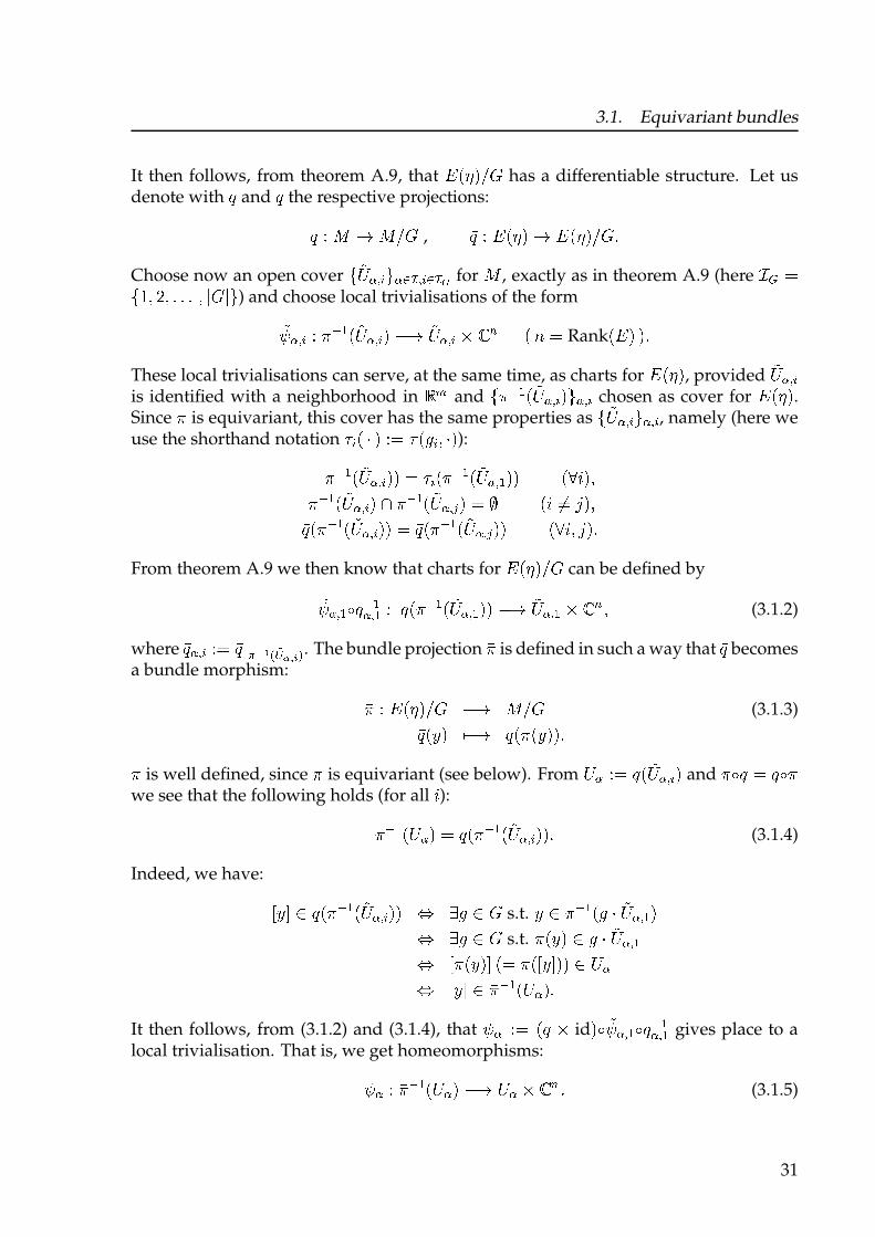
3.1. Equivariant bundles
It then follows, from theorem A.9, that ¢ £¤ ¥¦§ has a differentiable structure. Let usdenote with ¨ and © the respective projections:
¨ ª « ¬ « ¦§ , © ª ¢ £¤ ¥ ¬ ¢ £¤ ¥¦§ Choose now an open cover ®°± ²³ ´±µ¶ ²³µ¶ · for « , exactly as in theorem A.9 (here ¸ ¹ º®»¼ ½ ¼ ¼ ¾§ ¾´) and choose local trivialisations of the form
¿ ± ²³ ª À Á £°± ²³ ¥ ì °± ²³ Ä Å Æ £ Ç º Rank£¢ ¥ ¥These local trivialisations can serve, at the same time, as charts for ¢ £¤ ¥, provided
°± ²³is identified with a neighborhood in È É and ®À Á £°± ²³ ¥´± ²³ chosen as cover for ¢ £¤ ¥.Since À is equivariant, this cover has the same properties as ®°± ²³ ´± ²³, namely (here weuse the shorthand notation ʳ £ Ë ¥ ªº Ê £Ì³ ¼ Ë¥):
À Á £°± ²³ ¥¥ º ʳ £À Á £°± ²Â ¥¥ £Í Î¥ ¼À Á £°± ²³ ¥ Ï À Á £°± ²Ð ¥ º Ñ £Î Òº Ó ¥¼©£À Á £°± ²³ ¥¥ º ©£À Á £°± ²Ð ¥¥ £Í Î ¼ Ó ¥
From theorem A.9 we then know that charts for ¢ £¤ ¥¦§ can be defined by
¿ ± ²ÂÔ ©Á± ²Â ª ©£À Á £°± ²Â ¥¥ ì °± ²Â Ä Å Æ ¼ (3.1.2)
where ©± ²³ ªº ©¾Õ Ö× Ø ÙÚÛ ÜÝ Þ. The bundle projection ©À is defined in such a way that ©becomesa bundle morphism:
©À ª ¢ £¤ ¥¦§ ì « ¦§ (3.1.3)
©£ß ¥ àì ¨ £À £ß ¥¥©À is well defined, since À is equivariant (see below). From
°± ªº ¨ £°± ²³ ¥ and ©À Ô © º ¨ ÔÀwe see that the following holds (for all
Î):
©À Á £°± ¥ º ©£À Á £°± ²³ ¥¥ (3.1.4)
Indeed, we have:
áß â ã ©£À Á £°± ²³ ¥¥ ä åÌ ã § s.t. ß ã À Á £Ì Ë °± ²Â ¥ä åÌ ã § s.t. À £ß ¥ ã Ì Ë °± ²Âä áÀ £ß ¥â £º ©À £áß â¥¥ ã °±ä áß â ã ©À Á £°± ¥
It then follows, from (3.1.2) and (3.1.4), that¿± ªº £¨ Ä id¥Ô¿± ²ÂÔ ©Á± ²Â gives place to a
local trivialisation. That is, we get homeomorphisms:
¿± ª ©À Á £°± ¥ ì °± Ä Å Æ (3.1.5)
31

3. G-spaces and Projective Modules
Let us check that æç is well defined. We have:èé êë ì èéí ë î ïð ñ ò so that éí ì ð ó é êî ç ôéí õ ì ç ôð ó é êõ ì ð ó ç ôé ê õî èç ôéí õë ì èç ôé ê õë ö
That æç preserves fibers follows directly from the definition, eq. (3.1.3):ç ôé ê õ ì ç ôéí õ î æç ôæ÷ ôé ê õõ ì ÷ ôç ôé êõõì ÷ ôç ôéí õõì æç ôæ÷ ôéí õõ ö
Now, what the theorem asserts is that for a ò-bundle ø the following holds:ù ø úû ÷ ü ôø ýò õ: þ ôø õ ÿ� þ ôø õýò
� � � ýò �whereas for a bundle � over
� ýò one has:ù ÷ ü ô� õýò ú � : ÷ ü ô� õ �� � � ýò öThese isomorphisms must be established. Transition functions for ø ýò are determinedby the condition �� �� � ê� ôè ë � õ ì ôè ë � ð� �� ôè ë õ õ ö (3.1.6)
They can be related to the transition functions of ø , �ð� ��� , as follows. Considerè ë ñ�� � �� and choose a representative ñ è ë. Then ñ ��� � ���� for some � � � . In
particular, there are elements ð � � ð� ñ ò such that ��� ì ð � ��� � and ���� ì ð� ��� � . From
the definition of
�� in terms of ��� � it then follows thatð� �� ôè ë õ ì ð � ê� �ð�� �� ô õ ð � ö (3.1.7)
Here, ð � is a shorthand notation for the action of the group element ð � on � � inducedby � through the local trivializations of the bundle. Eq. (3.1.7) is obtained in exactlythe same way as eq. (A.3), see also diagram (A.4). On the other hand, the transitionfunctions ð � �� �� for the pull-back bundle ÷ ü ôø ýò õ are, by definition,ð � �� �� ô õ ì ð� �� ôè ë õ ö (3.1.8)
This shows the equivalence of ø with ÷ ü ôø ýò õ. Equations (3.1.7) and (3.1.8) give placeto a bundle isomorphism � � ø � ÷ ü ôø ýò õ, and it is easy to check that, with respectto the ò-action naturally defined on ÷ ü ôø ýò õ (see eq. (3.1.1)), � is ò-equivariant. Thismeans that ø and ÷ ü ôø ýò õ are also equivalent as equivariant bundles. The isomorphism� �ì ÷ü ô� õýò is established in a similar way.
32
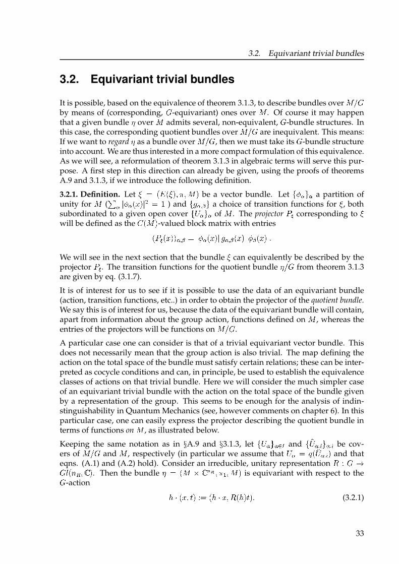
3.2. Equivariant trivial bundles
3.2. Equivariant trivial bundles
It is possible, based on the equivalence of theorem 3.1.3, to describe bundles over � !by means of (corresponding, !-equivariant) ones over � . Of course it may happenthat a given bundle " over � admits several, non-equivalent, !-bundle structures. Inthis case, the corresponding quotient bundles over � ! are inequivalent. This means:If we want to regard " as a bundle over � ! , then we must take its !-bundle structureinto account. We are thus interested in a more compact formulation of this equivalence.As we will see, a reformulation of theorem 3.1.3 in algebraic terms will serve this pur-pose. A first step in this direction can already be given, using the proofs of theoremsA.9 and 3.1.3, if we introduce the following definition.
3.2.1. Definition. Let # $ %& %# '( ) ( � ' be a vector bundle. Let *+, -, a partition ofunity for � (., /+, %0 ' /1 $ 2 ) and *3, 45 - a choice of transition functions for # , bothsubordinated to a given open cover *6, -, of � . The projector 78 corresponding to #will be defined as the 9 %� '-valued block matrix with entries%78 %0 '', 45 $ /+, %0 ' / 3, 45 %0 ' /+5 %0 ' /:We will see in the next section that the bundle # can equivalently be described by theprojector 78 . The transition functions for the quotient bundle " ! from theorem 3.1.3are given by eq. (3.1.7).
It is of interest for us to see if it is possible to use the data of an equivariant bundle(action, transition functions, etc..) in order to obtain the projector of the quotient bundle.We say this is of interest for us, because the data of the equivariant bundle will contain,apart from information about the group action, functions defined on � , whereas theentries of the projectors will be functions on � ! .
A particular case one can consider is that of a trivial equivariant vector bundle. Thisdoes not necessarily mean that the group action is also trivial. The map defining theaction on the total space of the bundle must satisfy certain relations; these can be inter-preted as cocycle conditions and can, in principle, be used to establish the equivalenceclasses of actions on that trivial bundle. Here we will consider the much simpler caseof an equivariant trivial bundle with the action on the total space of the bundle givenby a representation of the group. This seems to be enough for the analysis of indin-stinguishability in Quantum Mechanics (see, however comments on chapter 6). In thisparticular case, one can easily express the projector describing the quotient bundle interms of functions on � , as illustrated below.
Keeping the same notation as in ;A.9 and ;3.1.3, let *6, -,<= and * >6, 4? -, 4? be cov-ers of � ! and � , respectively (in particular we assume that 6, $ @ % >6, 4? ' and thateqns. (A.1) and (A.2) hold). Consider an irreducible, unitary representation A B ! C!D %EF ( G '. Then the bundle " $ %� H G IJ ( ) K ( � ' is equivariant with respect to the!-action L M %0 ( N ' B$ %L M 0 ( A %L 'N ' : (3.2.1)
33

3. G-spaces and Projective Modules
Since O is trivial, all PQRS TU V equal the identity of W and, therefore, the transition functionsfor O XW are given by (compare equation (3.1.7))QU TR Y ZU [ ZR \ W] ^_` a b c (3.2.2)de f g\ QU TR ^de f c h i ^jklm ci ^jn cawith o and p depending on some choice of e q def (the product jklm jn is independentof this choice). Choosing a partition of unity rsU tU for u XW (with Supp sU v ZU andwUxy zsU ^de fc z{ h |, for
de f in u XW) we define, for every }, the following map:~U� ^e c Yh � sU ^de fca if e q PZU �� a otherwise � (3.2.3)
This is in fact a smooth function u \ � , because Supp sU v ZU and PZU Tl � ZU . Usingthe action, we can generate zW z functions from
~U Tl. These functions give a partitionof unity for u , with respect to the open cover rZUV tU Tn. To show this, let e be anyrepresentative of
de f q ZU . Then there is exactly one open set PZU T� , that contains e(the index � q r|a � � � a zW zt obviously depends on e). It follows that there is only onenon-vanishing term in the sum
w�x� z~U � ^jkl � e c z{ and from this we conclude:��x� z~U Tl ^jkl � e c z{ h z~U Tl ^jkl� � e c z{ h zsU ^de fc z{ ^e q PZU T� c �That means, �Uxy ��x� z~U � ^jkl � e c z{ h |a ^�e q u ca (3.2.4)
as claimed. Now we can write down the projector � corresponding to O XW , in such away, that only functions on u are used:�UR ^de fc h sU ^de fcQUR ^de fcsR ^de fc ^from definition � �� �|ch sU ^de fc �i ^jkln ci ^jm c�sR ^de fch �~U � ^jkln � e ci ^jkln c� �i ^jm c~R � ^jklm � e c�h �����x� ~U � ^Pjkl � e ci ^Pjklc�� ���x� ~R � ^jkl � e ci ^jc� �The entries of (the block ^} a � c of the) projector can be expressed in terms of the matrixcomponents of the representation. One obtains:��UR ^de fc�nm h ���x� ��x� ~U � ^Pjkl � e c~R � ^jkl � e c �i ^Pjkl ci ^jc�nmh �����l ����x� i � ^Pj c�n~U � ^Pjkl � e c� ���x� i ^jc�m ~R � ^jkl � e c� �34

3.3. Projective Modules
Introducing the functions (� ¡ , ¢ £ ¤ ¥¦£ § § § £ ¨© ª)«¬® ¯° ± ²³ ¨©´µ ´ ¶·¸¹ º » ¯¼±® «¬ ½ ¯¼¾¿ À ° ±£ (3.2.5)
we obtain a more compact expression for the entries of the projector:Áˆ ¯Ä° űƮ ³ ´µ Ǩǩ ÈɶÊË¿ «¬Ê ¯° ±«Ã »Ê® ¯° ±§ (3.2.6)
The relevance of this formula, for us, is the following. The possibility of describingvector bundles by means of projectors (as the one from definition 3.2.1) comes fromthe Serre-Swan theorem, that establishes an equivalence between categories of vectorbundles on one hand and of finitely generated, projective modules on the other (thisequivalence will be discussed in some detail in the next section). The usefulness of eq.(3.2.6) is that we have a vector bundle Ì Íµ over the quotient space Π͵ but, using theSerre-Swan theorem, we know that this bundle can be equivalently described by thecorresponding projector. In our example, the bundle in question is the quotient bundleof a trivial bundle Ì defined on Î , which is
µ-equivariant. The
µ-action on the total
space is determined by a representation ofµ
. Since -as can be seen in eq. (3.2.6)- thecomponents of this projector can be expressed completely in terms of functions definedon Π(and not on Π͵), we are led to the idea that certain vector bundles over Π͵might be expressible in terms of functions defined on Π. This is in fact true, and insection 3.3 we will see how the
µ-action on Î naturally induces a decomposition ofÏ ¯Î ± into projective
Ï ¯Î ͵ ±-modules. The projectors describing these modules willbe shown to be precisely of the form we have just obtained in eq. (3.2.6).
3.3. Projective Modules
The purpose of this section is to obtain an alternative version of theorem 3.1.3 in termsof the spaces of sections associated with the bundles involved. There are mainly twomotivations for doing this.Ð As explained in the introduction, we are looking for a formulation of the quan-
tum mechanics of a system of identical particles in which the wave function isconsidered to be a section of a suitable vector bundle defined on the configura-tion space Ñ (eq.(1.1.2)). We remarked, at the end of chapter 2, that when theconfiguration space is multiply-connected, as is Ñ, it is a good strategy to con-
sider its universal cover, ÒÑ. In the case of “spin zero” quantum mechanics, a
standard procedure is to consider, at first, subsidiary functions ÓÔ ² ÒÑ Õ Ö . It isimportant to emphasize that such a function is not the physical wave function.The latter (call it
Ô) should have Ñ as its domain of definition and it might be that
35
3. G-spaces and Projective Modules
it is really not a function but a section on some bundle over ×. Although ØÙ is notthe physical wave function, some conditions can be imposed on it in order that
it represents the physical one. In that case, one says that ØÙ is “projectable” to ×.In order that such a function be “projectable”, it is required (for obvious physicalreasons) that, for Ú Û × and for any ØÚ in the fiber Ü ÝÞ ßÚ à (Ü denotes the projectionÜ á â× ã ×) ä ØÙ ßØÚ à äå depends only on the point Ú, independently of ØÚ. RestrictingØÙ in this way, we force its domain of definition to be “almost” ×, for if ØÚ Þ and ØÚåbelong to the same fiber Ü ÝÞ ßÚ à, ØÙ ßØÚ Þà and ØÙ ßØÚå à may still differ by a phase. Thesetwo points are related by an element æ of ç Þ ß×àè ( ØÚå é æ ê ØÚ Þ) and one can showë,that the phase can only depend on æ . The restriction on ØÙ takes the formØÙ ßæ ê ØÚ à é ì ßæ à ØÙ ßØÚ àí (3.3.1)
where ì is, as in theorem 1.1.1, a one dimensional unitary representation of ç Þ ß×à.In other words, ØÙ is required to be ç Þ ßî à-equivariant. It is in this sense that oneshould understand the statement, often found in the literature, that on multiply-connected spaces, “multiple-valued” functions are allowed. In this context, un-der multi-valuedness of
Ùone should understand equivariance (as expressed by
eq. (3.3.1)) of ØÙ . This somewhat confusing situation has, to our opinion, not beendiscussed in a clear and systematic way, and it leads to further confusion whenspin degrees of freedom are taken into account (see discussion in section 5.3). Thereformulation of theorem 3.1.3 we give in this section (see theorem 3.3.5 below)provides a suitable framework for handling the situation discussed above.ï The second reason is that this reformulation serves as a first step towards a for-mulation of the problem in only algebraic terms. Using the language of algebrasand modules might prove to be useful in the search for a relation between the(mainly geometric) configuration-space approaches to the Spin-Statistics relation,and the Field theoretical ones, in which proofs of the Spin-Statistics theorem areavailable. It would be very interesting to eventually find an interpretation of theanalytical proofs in geometrical terms. The relation of these proofs to, for exam-ple, the work of Finkelstein-Rubinstein[FR68] on topological solitons, is some-thing that has not been clarified. One of the difficulties is certainly the differenceof “languages” (the one algebraic/analytical, the other topological).
With the above remarks as motivation, let us recall two basic results that relate cat-egories of topological spaces with categories of algebraic objects. For ð a compactHausdorff topological space, the space ñ ßð à is an algebra that, by the Gelfand-Naimark theorem, carries all the information about the (topological) space ð . By thesame theorem, this correspondence between topological spaces and complex algebrasis bijective. Schematically, we have:ò
Recall that óô õö÷ acts on øö by Deck transformations.ùSee [Mor92] and references therein.
36

3.3. Projective Modules
úCompact Hausdorfftopological spaces û Gelfand-
Naimarkú
Unital, commutativeü ý-algebras û þ
An analogous result for vector bundles is also available: if ÿ is a vector bundle overthe compact space � , then it is well known that � �ÿ � carries the structure of a finitelygenerated and projective
ü �� �-module. The module multiplicationü �� � � � �ÿ � �� � �ÿ ��� � � �� � (3.3.2)
is defined by pointwise multiplication: �� ��� � � � �� � �� � (the easier notation� for the module product is usually used). The Serre-Swan theorem establishes thefollowing bijective correspondence:ú
Vector bundlesover M û Serre-
Swanú
Finitely generated,projective
ü �� �-modules û þThese two theorems (Gelfand-Neumark and Serre-Swan) provide complete equiva-lences between classes of topological objects on one side and of algebraic ones on theother. Let us, for the sake of concreteness, state the Serre-Swan theorem.
3.3.1. Theorem (Serre-Swan (cf.[Ser58],[Swa62])). Let � be a compact, finite dimensionalmanifold and let � be a
ü �� �-module. Then there exists a vector bundle ÿ �� �ÿ � � � � � �whose
ü �� �-module of sections � �ÿ � �� � � � � �ÿ � � � is continuous and � �� id� isisomorphic to � if and only if � is finitely generated and projective.
In order to obtain an algebraic formulation of theorem 3.1.3, all that must be done, inview of theorem 3.3.1, is to replace all assertions about the relations between ÿ and ÿ ��by assertions about the corresponding spaces of sections, � �ÿ � and � �ÿ �� �. This taskcan be easily performed once one realizes that the pull-back of a vector bundle, at thealgebraic level, can be obtained from the tensor product of appropriate algebras andmodules. The precise assertion is formulated in theorem 3.3.2, but before proving it wewill make some remarks from which the proof follows quite naturally.
Let � � � � � � � (3.3.3)
be a �-action on the topological space � . It, in turn, induces an action � � ü �� � �ü �� � � �� � � � �� � �, where
�� � ��� � � � ��� �� �� �� � �� �� � � þ (3.3.4)
Analogously, for a �-bundle ÿ with corresponding action � � � � �ÿ � � � �ÿ �, anaction on the space of sections, � �ÿ �, will be induced, as follows: For ! � �ÿ � and� ! � , � � � � � �ÿ � is defined through
�� ��� � � � � �� �� � �� þ (3.3.5)
37
3. G-spaces and Projective Modules
The two actions (on " #$ % and on & #' %) are related, through the module multiplication,as follows: ( ) #*+ % , #( ) * %#( ) + %- (3.3.6)
Consider now a continuous map . / $ 0 1 and a vector bundle 2 over 1 . We seeka characterization of the " #$ %-Module & #.32 % where, instead of .32 , only the " #1 %-Module & #' % is used. In other words, what we are looking for is a " #$ %-module whichis isomorphic to & #.32 %, but constructed from the data ., " #1 %, " #$ % and & #2 % (no ex-plicit mention of .32 ). This means that somehow we have to compare & #2 % with & #.32 %.But & #2 % and & #.32 % are modules over different rings (" #1 % and " #$ %, respectively),so it is only possible to compare them either by considering & #.32 % as a " #1 %-module,or the other way around, that is, by regarding & #2 % as a " #$ %-module. Both alterna-tives are possible, but only through the second one do we obtain the isomorphism weare looking for.
To see this, notice that . induces a ring homomorphism
.3 / " #1 % 40 " #$ %5 640 .35 /, 5 7. -This homomorphism can be used to obtain a " #1 %-module structure on & #.32 %:
" #1 % 8 & #.32 % 40 & #.32 % (3.3.7)# 5 9 : % 640 5 ) : /, #.35 %: -For any given section ; < & #2 %, we define a section
.3; / $ 40 = #.32 % (3.3.8)> 640 #> 9 ; 7. #> %%-This gives place to a homomorphism of " #1 %-modules? @ / & #2 % 40 & #.32 % (3.3.9); 640 ? @ #; % A .3; -? @
is clearly a " #1 %-linear map:? @ #5 ) ; % , .3 #5 ) ; % BC DC DE F, #5 7.%.3; BC DC DGF, 5 ) .3; , 5 ) ? @ #; %-But it is also clear that
? @is not, in general, an isomorphism. Indeed, although we
may choose generators for & #.32 % of the form ; HI , ? @ #;I %, we see from Im#? @ % ,JK I #5I7.%; HI L 5I < " #1 %M that? @
is not surjective in general, because the elements inthe image module are only linear combinations of the generators over the subspace.3 #" #1 %% of " #$ %. In other words: The generators ; HI may be multiplied only by el-ements of " #1 %. We thus see that a change of ring, performed with the help of thetensor product, is necessary. With the previous remark as motivation, we setN / " #$ % OP BQ F & #2 % 40 & #.32 % (3.3.10)R
S *S O ;S 640 RS *S? @ #;S %-
38

3.3. Projective Modules
3.3.2. Theorem (cf. [GBVF01]). The map defined through (3.3.10) is an isomorphismT UV W XY Z[ \ ] U^ W _ ] Uab^ Wof
T UV W-modules.
Proof. (i) c is aT UV W
-module homomorphism:
c Ud e f Udg X h WW ` c UUd edg W X h W ` d edgi Uh W ` d ec Udg X h Wj(ii) If
] U^ Wis generated by khl mln eoppp oq , then
] Uab^ Wis generated by ki Uhl Wmln eoppp oq :
The fiber^r
over s t u is generated by the vectors khl Us Wm. From
ab^v ` kw m x ^y Zv \it is
then clear that the vectors kUw z hl Ua Uw WWWmlgenerate the fiber
ab^v. The assertion follows
from this fact, together with (3.3.9).
(iii) c is surjective:
Given { t ] Uab^ W, there exist -because of (ii)- functions
d e z j j j z dq t T UV Wsuch that{ ` | l dli y Uhl W
.This implies { ` c U| l dl X hl W.
(iv) c is injective: Clear if] U^ W
is a free module, because in that case there exists abasis. In the general case, there exists some } such that
] U^ ~ } Wis a free module, so
that there is an isomorphism c� � T UV W XY Z[ \ ] U^ ~ } W � ] Uab U^ ~ } WWjThe inclusions� � T UV W X ] U^ W �� T UV W X ] U^ ~ } W
and � � ] Uab^ W �� ] Uab^ W ~ ] Uab} Ware injective and,
moreover, � �c� ` c��: c must also be injective.
If -for the situation in (3.3.3)- we set u � V ��and
a � � � V � V ��in thm. 3.3.2,
then we can construct an injectiveT UV �� W
-module homomorphism
c� � ] U^ W �� ] U� b^ Wzas follows. Recall that
�acts on
T UV Wby (3.3.4). In the next section it will be shown
that this action induces a decomposition ofT UV W
intoT UV �� W
-submodules (see eq.(3.4.27)). All that we need from this result is the fact that
T UV Wmay be decomposed in
the form T UV W ` T UV W� ~ � zwhere
T UV W�stands for the subalgebra kd t T UV W � � f d ` d � � t � m
of�
-invariantfunctions and also that
�has the structure of a projective
T UV �� W-module. Noticing
that the algebrasT UV W�
andT UV �� W
are isomorphic, we obtain:T UV W XY Z� �� \ ] U^ W _ ] U^ W ~ �� XY Z� �� \ ] U^ W� j(3.3.11)
Denote with� � ] U^ W �� T UV W XY Z� �� \ � U^ W
the corresponding inclusion. Making useof thm. 3.3.2 we can put c� �` c�� and in that way obtain the desired result.
3.3.3. Remark. It is important to notice that, although c� U] U^ WWand
] U^ Ware isomor-
phic asT UV �� W
-modules, c� U] U^ WWis actually contained in
] U� b^ W. This means that,although every section from
] U^ Wcan be “replaced” by one from c� U] U^ WW
, sectionsfrom c� U] U^ WW
may only be multiplied by functions inT UV W�
, if we want to identifyc� U] U^ WWand
] U^ Was modules.
39

3. G-spaces and Projective Modules
3.3.4. Remark. From Eqns. (3.3.10) and (3.3.11) we see that �� �� � � � � �� �.It is possible to give a better description of the image of �� . In fact, one finds that�� �� �� �� equals the space of invariant sections of the pull-back bundle:
3.3.5. Theorem.
� �� � �� �� �� �� �� � �� �� � � ¡� ¢£ ¤ � �� � � ¥ ¦ § £ � £ ¨ ¦ ¤ �©ªProof. The first equality is clear, since �� is an injective homomorphism. Every sectionfrom �� �� �� �� is of the form � � , with � ¤ � �� �. From the definition of � � (see Eq.(3.3.8)) and from the form of the action « induced induced on � � by � (see Eq.(3.1.1)) itfollows that a section of the form � � is invariant:
�¦ § � � � �¬ � � « �¦ ®¯ § ¬ ° � ±� �¦ ®¯ § ¬ ��²³ ´¯´¯µ� �¬ ° � ±� �¦ ®¯ § ¬ ��� �¬ ° � ±� �¬ ��� � � �¬ �ªConversely, every invariant section must be of the form � � : Given £ ¤ � �� � �, there isa continuous map ¶ ¡ · ¸ ¹ �� � with º ±¶ � � and £ ¡ ¬ »¸ �¬ ° ¶ �¬ ��. If £ is invariant,then ¶ �¦ §¬ � � ¶ �¬ � holds for all ¦ in ¼ , so that one can define a section � ¤ � �� � through� �½¬ ¾� ¡� ¶ �¬ �, for which £ � � � holds.
3.4. Decomposition of ¿ ÀÁ ÂLet ¼ be a finite group. Denote with ÃÄ ¡ ¼ ¸ Gl�Å Ä � �Æ � Ç° ª ª ª ° È � its irreduciblerepresentations. A general representation à ¡ ¼ ¸ Gl�É � can always be reduced, i.e.,É can be written in the form
É � É ¯ Ê § § § Ê É Ë ° (3.4.1)
where every subspace É Ì is invariant under ¼ and can be reduced further,
É Ì � É Ì Ê § § § Ê É ÌÍÎ ° (3.4.2)
in such a way that dim�É ÌÏ � � ÐÌ ¡� dim�Å Ì � for all Ñ � Ç° ª ª ª ° ÒÌ (ÒÌ � multiplicityof ÃÌ in É ). In particular, for a given Ó , all the representations à ¥Ô ÎÕ are equivalent to ÃÌ .The decomposition of É then takes the form
É �� Ò ¯Å ¯ Ê § § § Ê ÒË Å Ë ª (3.4.3)
Since all subspaces É ÄÏ (for Æ fixed) are equivalent as representations, one is interested infinding a basis for every É ÄÏ with the property that the representing matrices are all thesame, for Ñ � Ç° ª ª ª ° Ò Ä. Obviously such basis do exist, so the question would ratherbe: How can one find such basis systematically?.
40

3.4. Decomposition of Ö ×Ø Ù3.4.1. Remark. The problem of determining such “symmetry respecting” basis isclosely related to the fact that, in contrast to eq. (3.4.1), the decomposition in eq. (3.4.2)is not unique. As we will see, after a concrete choice for the representing matrices ofÚÛ
has been made, it is possible to define certain operators that allow one to find thosesymmetry-respecting basis. Of course, a choice of basis for the different subspacesamounts to writing down an explicit decomposition of Ü Û
. It is clear from this point ofview that the decomposition cannot be unique.
In the case of the regular representation, the construction of the operators mentioned inthe previous remark is particularly clear. Since the formulae obtained in this case canbe applied in general, we want to discuss this example in detail.
3.4.2. Definition. For Ý a finite group, let Þ ×Ý Ù denote the vector space of complexfunctions on Ý (it dimension equals the order of the group, ßÝ ß). The regular representa-tion, àá , is the representation on Þ ×Ý Ù induced by the group multiplicationâàá ×ã Ùä å ×æÙ çè ä ×ãéêæÙ ×ä ë Þ ×Ý Ùì ã í æ ë Ý Ùî3.4.3. Remark. It is a well-known fact that the regular representation contains all irre-ducible representations of Ý , each one with a multiplicity equal to its dimension:
Þ ×Ý Ù ïè ðñòóêôòõ ò
(3.4.4)
In particular, for the dimension of Þ ×Ý Ù, we have:
dim×Þ ×Ý ÙÙ è ðöòóêôòdim×õ ò Ù è ðöòóê ×ôò Ù÷ î (3.4.5)
Although an additional decomposition of ôòõ òis not canonically given, it is possible
to, in a sense, “factor out” these subspaces, if one regards Þ ×Ý Ù as a representation ofÝ ø Ý . For this purpose we consider a Ý ø Ý-action on Ý , defined by
×Ý ø Ý Ù ø Ý ù Ý××ú ê í ú÷ Ù í û Ù üù ú êûú éê÷ î (3.4.6)
The representation induced by this action on Þ ×Ý Ù will be denoted with ýþá .
Another Ý ø Ý representation can be defined as follows. Let ÿÚò (� è � í î î î í� ) be the
representation induced byÚò on the dual space õ ò�
: × ÿÚò ×ú Ù� Ù×� Ù çè � ×Ú ò ×ú éêÙ� Ù ×� ëõ ò í � ë õ ò� í ú ë Ý Ù. It follows thatÚò � ÿÚò is an irreducible Ý ø Ý representation onõ ò � õ ò�
. This representation can be realized inside Þ ×Ý Ù. This is a consequence of thefollowing fact:
3.4.4. Theorem. The map � ò ç õ ò � õ ò� ù Þ ×Ý Ù, defined by� ò ×� � � Ù ×ú Ù çè � ×Ú ò ×ú éê Ù� Ùí (3.4.7)
is Ý ø Ý-equivariant.
41
3. G-spaces and Projective Modules
Proof. For � �� � � � , � � � � � � � �� and � � , we have:�� �� � � � � � �� �� � � �� ��� � �� � ��� ����� �� �� � ��� ����� ��� �� !��� � ���� � ��� �� !� �� ! ���� �� �� � ���� �� ! � � �� �"#$ � ���� �� � ��� �� �� �� � � � �� �� � ��� �� �%3.4.5. Theorem. The decomposition of & �� � into irreducible � � �-representations is& �� � '� ()�*! �� � � �� % (3.4.8)
Proof. It follows from theorem 3.4.4, together with Schur’s lemma (since�� is injective),
that every representation�� � ��� (i=1, % % % ,N) is contained in & �� �, that is, we have an
equivalence of representations: �� � � � �� � � � ��� � ' �& �� � +Im,-. / "#$ +Im,-. / �. The direct
sum of all � � � � �� must appear as a sub-representation in & �� �, since�� � ��� ' �0 � ��0
precisely when 1 � 2 . Therefore, equation (3.4.8) must hold -as an isomorphism of� � � representations- since dim�3 �� � � � �� � � 4 � 56� � dim�& �� ��.From the previous theorem we learn that the two � � �-representations, �& �� � "#$ �and �7 � �� � � � �� � 7 � ��� � ��� ��, are equivalent. The isomorphism is given explicitlyby the sum
� 8� 7 � �� of all�� from theorem 3.4.4, so that, if we choose a basis 9: ;.<= >=
for � �, it is now possible to write every element of & �� � as a sum over every of itscomponents in the subspaces � � � � ��.Let 9 �: ;.<= >= be the dual basis of � ��, induced by 9: ;.<= >= . Denote with ? ;.< �� � the represent-ing matrices of
��, with respect to 9: ;.<= >= .Every function @ & �� � can be written in the form @ � 4 AB$ @ �� �CA , where CA standsfor the characteristic function of � (CA �D� equals one if � � D, zero otherwise). We areseeking now those coefficients E�= F= G for which the following holds:CA � � H (I�*! J.I=F= G* ! E�= F= G : ;.<= � �: ;.<= G K % (3.4.9)
42

3.4. Decomposition of L MN OInserting (3.4.7) into (3.4.9), leads to:PQ MRO ST U V WXYZ[ \]X^_^`Z [ a Y _^ ` b c]d^ e fb c]d^ ` g MR OT WXYZ[ \]X^_^ `Z [ aY _^ ` UY Mb c]d^ e fb c]d^ ` O MR OT WXYZ[ \]X^_^ `Z [ aY _^ ` fb c]d^ ` MhY MRi[ Ob c]d^ OT WXYZ[ \]X^_^ ` _^ ``Z [ aY _^ ` j c]d^ `` _^ MRi[ O fb c]d^ ` Mb c]d^ `` OT WXYZ [ \]X^_^ `Z [ aY _^ ` j c]d^ ` _^ MRi[O k
Xlmn j co dp _q MR OPQ MR O T WXYZ[ \]X^_^ `Z [ a Y _^ ` Xlmn j co dp _q MR Oj c]d^ ` _^ MRi[ Or st uZv] wo vx wy vz wy ` {| {}ok
aY _^ ` T ~Y�� �j c]d^ _^ ` M� O (3.4.10)
It then follows, for � in � M� O:� M� O T Xlmn � MROPl (3.4.11)T Xlmn � MROU V WXYZ[ ~Y�� � \]X^_^ `Z [ j c]d^ _^ ` MR Ob c]d^ e fb c]d^ ` g M� OT Xlmn � MRO WXYZ [ ~Y�� � \]X^_^ `Z [ j c]d^ _^ ` MR Oj c]d^ ` _^ M� i[ OT WXYZ[ \]XZ [ ~Y�� � Xlmn j c]d^ _^ MRi[O� MRi[� O�From this formula we learn that the operator~Y�� � \ ]XZ [ XQmn j c]d^ _^ M� i[O� � M � O (3.4.12)
43
3. G-spaces and Projective Modules
is the projection operator � �� � � � � � � �� . Because of the (vector space) isomorphism� � � � �� � dim�� � �� � � ��� �, one is led to consider, in (3.4.12), only the single termsin the sum over � : ���� � ���� � ���� �� �� ¡ �� ¢ � £ �¤ (3.4.13)
We will now see that these are still projection operators, which turn out to be veryuseful for the algebraic description of �-bundles and of their quotients.
Before concluding this section, let us come back to remark 3.4.1, in order to furtherexplain the role played by the operators defined through the formula (3.4.13) in theconstruction of a symmetry-preserving basis.
Consider, once again, a general representation, ¥, of � . The representation space ¦ isto be decomposed, as in equations (3.4.1) and (3.4.2), into irreducible subspaces. Fora given § , let us assume that the representation ¥¨ appears in this decomposition and,moreover, that a symmetry-preserving basis ©ª« �¬ ¡®«®¯° ±¡®¬®²° for ¦ ¨
is known.
That means: For ³ fixed, ©ª« �¬ ¡®¬®²° is a basis for ¦« and¥ �� �ª« �´ � �¬ µ �° �¬ �´ �� �ª« �¬ ¶holds, i.e., the representing matrices in the space spanned by ©ª« �¬ ¬ are the same forall ³. Defining now, in accordance with our previous considerations, the operators· �° �¬ �´ � �¨�� ����� µ �° �¬ �´ �� ¡ �¥ �� �¶ (3.4.14)
we obtain, from the orthogonality relations for the matrix components of irreduciblerepresentations, · �° �¬ �´ ª« �¬ ¸ � ¹¬ �¬ ¸ ª« �¬ ¤ (3.4.15)
The array �ª ¡�¬ ¶ ªº �¬ ¤ ¤ ¤ ¶ ª¯° �¬ � is transformed by· �° �¬ �´ into �ª¡�´ ¶ ªº �´ ¤ ¤ ¤ ¶ ª¯° �´ �, componen-
twise. All other vectors ª« �¬ ¸ (» ¼ ½� ») in the basis of ¦ ¨belong to the kernel of
· �° �¬ �´ . In
this basis,· �° �¬ �´ is given by a matrix whose �¾¼ ¶ » ¼ � component equals ¹´ �´¸ ¹¬ �¬ ¸ . From this,
one concludes that the rank of· �° �¬ �´ is ¿¨ .
Since ¥¨ appears in the decomposition of ¦ , there exists À ¡ Á ¦ with  ¡�¡ Ã� · �° �¡�¡À ¡ ½� Ä.Moreover,  ¡�¡ must be a linear combination of the form ¡�¡ � Å¡ª¡�¡ Æ Åº ªº �¡ Æ ¢ ¢ ¢ Æ Å¯° ª¯° �¡ ¶ (3.4.16)
because in every ¦« ,· �° �¬ �¬ projects on the » ÇÈ basis vector. Applying
· �° �¡�¬ (» � É ¶ ¤ ¤ ¤ ¶ �¨ )to  ¡�¡ we obtain further vectors  ¡�¬ Ã� · �° �¡�¬  ¡�¡ that, because of (3.4.15), are given by
44
3.4. Decomposition of Ê ËÌ Ía linear combination of the vectors ÎÏÐÑ Ò Ó Ó Ó Ò ÎÔÕ ÐÑ , with the same coefficients Ö× as in(3.4.16): Ø ÏÐÑ Ù ÔÕÚ×ÛÏ Ö× Î× ÐÑ Ó (3.4.17)
3.4.6. Theorem. The vectors
Ø ÏÐÏ Ò Ó Ó Ó Ò Ø ÏÐÜÕ form a basis for ÝÞ . When written in terms of thisbasis, the representing matrices are exactly the same as for ßÎ× ÐÑ àÑ .Proof. Ý Ëá ÍØ ÏÐÑ Ù Ý Ëá Í âÔÕÚ×ÛÏ Ö× Î× ÐÑã (3.4.18)Ù ÜÕÚäÛ Ï å æÕ çä ÐÑ Ëá Í ÔÕÚ×ÛÏ Ö× Î× Ðä (3.4.19)Ù ÜÕÚäÛ Ï å æÕ çä ÐÑ Ëá Í
Ø ÏÐä Ó (3.4.20)
Since è æÕ çÏÐÏ has rank éÞ , we can still find other éÞ ê ë independent vectors ì× Ëí Ùî Ò Ó Ó Ó Ò éÞ Í such that è æÕ çÏÐÏì× ïÙ ð. Defining nowØ× ÐÑ ñÙ è æÕ çÏÐÑì× Ëò Ù ëÒ Ó Ó Ó Ò óÞ Í Ò
we obtain a symmetry-preserving basis for ô Þ, since the assertion of proposition 3.4.6
remains valid for í Ù î Ò Ó Ó Ó Ò óÞ :Ý Ëá ÍØ× ÐÑ Ù ÜÕÚäÛ Ï å æÕ çä ÐÑ Ëá ÍØ× Ðä Ó
The meaning of the operators è æÕ çÑ Ðä becomes clearer by arranging the basis vectorsßØ× ÐÑ à× ÐÑ in a “matrix”, as follows:
45
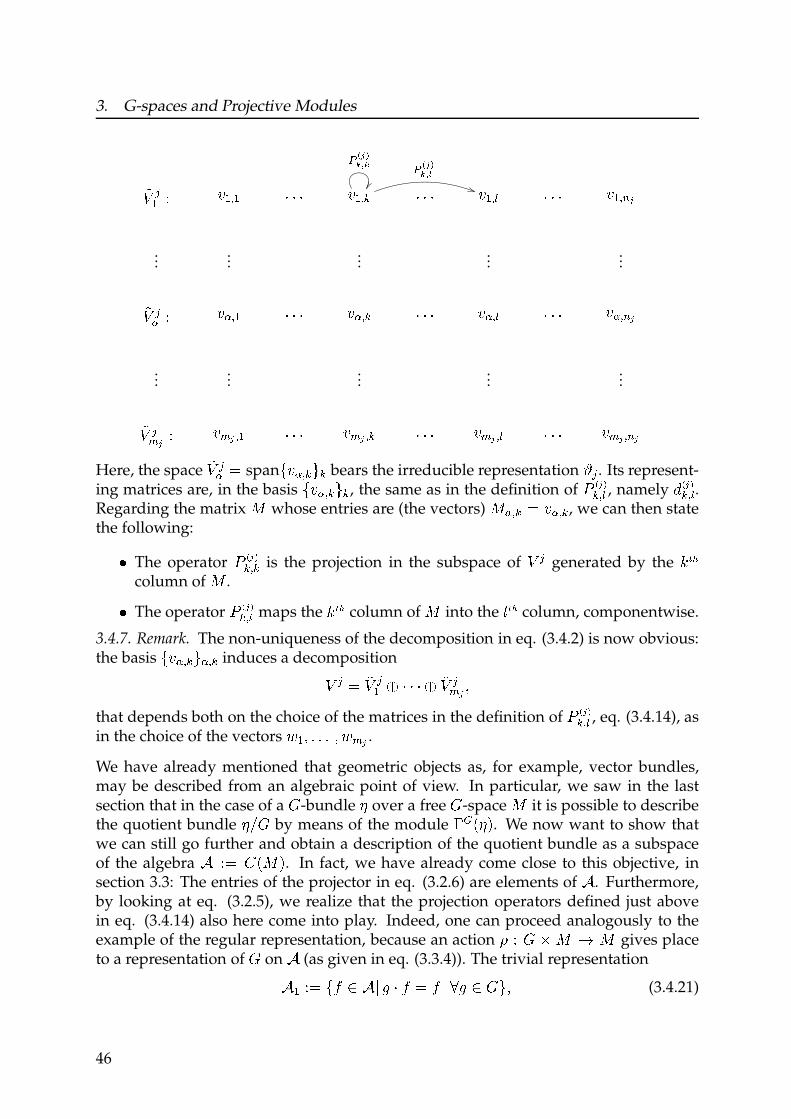
3. G-spaces and Projective Modules
õö ÷ø ù ú øûø ü ü ü ú øûýþ ÿ� �� �� þ ÿ� �� ��ü ü ü ú øû� ü ü ü ú øû��...
......
......õö ÷� ù ú� ûø ü ü ü ú� ûý ü ü ü ú� û� ü ü ü ú� û��
......
......
...õö ÷�� ù ú�� ûø ü ü ü ú�� ûý ü ü ü ú�� û� ü ü ü ú�� û��Here, the space
õö ÷� spanú� ûý �ý bears the irreducible representation �÷ . Its represent-
ing matrices are, in the basisú� ûý �ý , the same as in the definition of ÿ� �ý û� , namely � ÿ� �ý û�.
Regarding the matrix � whose entries are (the vectors) �� ûý ú� ûý , we can then statethe following:� The operator ÿ� �ý ûý is the projection in the subspace of
ö ÷generated by the � ��
column of � .� The operator ÿ� �ý û� maps the � �� column of � into the � �� column, componentwise.
3.4.7. Remark. The non-uniqueness of the decomposition in eq. (3.4.2) is now obvious:the basis
ú� ûý �� ûý induces a decompositionö ÷ õö ÷ø � ü ü ü � õö ÷�� �that depends both on the choice of the matrices in the definition of ÿ� �ý û� , eq. (3.4.14), asin the choice of the vectors � ø � � � � � ��� .We have already mentioned that geometric objects as, for example, vector bundles,may be described from an algebraic point of view. In particular, we saw in the lastsection that in the case of a �-bundle � over a free �-space � it is possible to describethe quotient bundle � �� by means of the module �� �� �. We now want to show thatwe can still go further and obtain a description of the quotient bundle as a subspaceof the algebra ù ! �� �. In fact, we have already come close to this objective, insection 3.3: The entries of the projector in eq. (3.2.6) are elements of . Furthermore,by looking at eq. (3.2.5), we realize that the projection operators defined just abovein eq. (3.4.14) also here come into play. Indeed, one can proceed analogously to theexample of the regular representation, because an action " ù � # � $ � gives placeto a representation of � on (as given in eq. (3.3.4)). The trivial representation ø ù % & '( ü % % )( & � �� (3.4.21)
46

3.4. Decomposition of * +, -is contained in . as a subalgebra. As we have already seen, there is an algebra isomor-phism * +, /0 - 1 2 3 (in section 3.3 the notation * +, -4 was used instead of . 3). Letus consider eq.(3.2.5). There we obtained, from a single function (567), 89 : 89 newfunctions, with the help of the representation ; . The definition of these functions is, toa certain extent, singled out by the explicit form of the projector. This can be seen ineq. (3.2.6). In their form they are similar to the operators defined in eq. (3.4.14) and forthis reason we will make the following ansatz:
Let ; be an 89 -dimensional, irreducible, unitary representation of 0 . For < = > ?@A= B B B = 89 C set D 9EF G . H .I JH D 9EF I =where D 9EF I +K - GL 89M0 MNOPQ ;EF +RS3-I +RS3 T K - +K ? , -B (3.4.22)
The behavior of these functions under the 0-action is easy to establish. For example,for
I ? . L * +, - and R ? 0 , we have:UR T +D 9EF I -V +K - L +D 9EF I - +RS3 T K -L 89M0 MNWOPQ ;EF +XRS3-I ++R XR-S3 T K --L 89M0 M NOYPQ ; EF +RZS3R -I +RZS3 T K -L [\N]^3 ;]F +R - 89M0 M NOYPQ ; E] +RZS3 -I +RZS3 T K -L [\N]^3 ;]F +R -DE] I +K -BSummarizing,
R T +D 9EF I - L [\N]^3 ;]F +R -D 9E] I B (3.4.23)
If we keep < fixed, then the 89 functions@D 9E _3I = B B B = D 9E _[\ I C form (in case they do not
vanish everywhere) a basis for the representation ; , exactly as in thm. 3.4.6. On theother hand, letting first R act on
I, we obtainD 9EF +R T I - L [\N]^3 ; E] +R -+D 9]F I -B (3.4.24)
47

3. G-spaces and Projective Modules
The maps ` abc are, analogously to the d ef gh i , orthogonal to each other: For j k and jl twoirreducible, unitary representations, one has` a mbh ` anop q ra m san rho ` a mbp t (3.4.25)
Let u be any function in v . It is to be expected, from eqns. (3.4.11) and (3.4.12), that umay be written in the following form:
u q wapxwby k ` abb u z (3.4.26)
where the first sum is performed over all inequivalent, irreducible representations. Letus check that this is indeed the case:wa
pxwbyk ` abb u {| } q wapxwby k ~a�� �w��� j �bb {� }u {��k � | }q wa w��� ~a�� � pxwby k j �bb {� }� �� �� �x �� � u {��k � | } {~a q �a {�}}
q w��� ��� �wa �a {�}��a {� }� �� �y �� ��� �� u {��k � | }q u {| }t
This shows that we have found the following decomposition of v :v q �asb v a sb z (3.4.27)
with va sb �q ` abb {� }.The trivial representation v k appears exactly once in the decomposition. As statedabove, it is an algebra isomorphic to � {� �� }. It is clear that the spaces va sb are v k-modules, since � � u q u for � � �
and u � v k, so it follows that u � � va sb u �v k z � � va sb. What is not yet so clear is whether these modules are finitely generatedand projective.
3.4.8. Theorem. The v k-module va sb �q ` abb {v } is, for any unitary, irreducible representa-tion j and ¡ � ¢�z t t t z ~a £, finitely generated.
Proof. For u � va sb we have ` abb u q u ; that means:~a�� �w��� j �bb {� }u {��k � | } q u {| } | � � t48
3.4. Decomposition of ¤ ¥¦ §Let now ¨©ª «ª¬ be, as in section 3.2, a partition of unity for ¦ ®¯ , subordinated to thecover ¨°ª «ª¬ . Because of the isomorphism ¤ ¥¦ ®¯ § ±² ³ ´, we may regard ©ª as anelement from ³ ´. In particular, the notations ©ª ¥µ § (© ¶ ³ ´) and ©ª ¥·µ ¸§ (© ¶ ¤ ¥¦ ®¯ §)will be used interchangeably, according to convenience. It is clear, from eqns. (3.2.5)and (3.4.22), that ¹ªº» ² ¼ ½º» ¹ª ¾ (3.4.28)
holds, with
¹ª¾ as defined in the example of section 3.2. One also sees that (with thesame conventions as in section 3.2)
Supp¥¿ ©ª § À Á ´ ¥°ª § ² ÃÄÅ» Æ ´ Ç°ªÈ É (3.4.29)
Furthermore, ¿ ©ª can be “split” in Ê Ë Ì¯ Ì different functions ¿ªÍ , in such a way that
©ª ¿ ² Îϻƴ ¿ªÈ Ð mit Supp¥¿ªÈ § Ñ Ç°ªÈ ÒÓ (3.4.30)
holds. Namely, defining
¿ªÈ ¥µ § Ô² Õ ¥©ª ¿ § ÖÖ ×ØÙÈ ¥µ §Ð in case µ ¶ Ç°ªÈÚ Ð otherwise Ð (3.4.31)
we see that (3.4.30) is satisfied, since for Û fixed all Ç°ªÈ are disjoint. The maps ¿ªÈare well-defined, continuous functions, because Supp ¥©ª ¿ § À Ç°ªÈ . By defining the(invariant) functions ¿ ÜªÈ Ô² ÏÝ¬Þ ß à ¿ªÈ Ð (3.4.32)
the following identity is then obtained:ÏÝÈ ¬Þ ¿ ÜªÈ ¥µ §¹ª ¾ ¥ß´» à µ § ² ©ª ¥·µ ¸§á ¿ ¥µ §É (3.4.33)
It is enough, in order to check (3.4.33), to consider µ ¶ Ç°ªâ , since both sides of theequation have support in Á ´ ¥°ª § ² ãλ Æ ´ Ç°ªÈ . One then obtains:ÏÝÈ ¬Þ ¿ ÜªÈ ¥µ §
¹ª ¾ ¥ß´» à µ § ² ¿ ܪ⠥µ §¹ª ¾ ¥ß´ä à µ §² ¿ ܪ⠥µ §©ª ¥·µ ¸§² ÏÝÈ ¬Þ ¿ªâ ¥ß´» à µ §©ª ¥·µ ¸§² ¿ªâ ¥µ §©ª ¥·µ ¸§² ©ª ¥·µ ¸§á ¿ ¥µ §É49

3. G-spaces and Projective Modules
Summing over å,æç æèé êë ì íçé îï ðñç ò îóôõö ÷ ï ð ø æç ùç îúï ûðü ì îï ð ø ì îï ðýThat means
ì ø æçêþ æèé êë ì íçé îóö ÷ ñç ò ð ÿso that
ì îï ð ø � ��� ì îï ð ø �� ��� �æçêþ æèé êë ì íçé îóö ÷ ñç ò ð�� îï ðø �æçêþ æèé êë � ��� �ì íçé îóö ÷ ñç ò ð�� îï ðø æçêþ æèé êë ì íçé îï ð �� ��� îóö ÷ ñç ò ð� îï ðø æçêþ æèé êë ì íçé îï ð æ� � õ �� îóö ð �� ���ñçò� �� �� ���� � îï ðø æçêþ æ� � õ �æèé êë ì íçé îï ð �� îóö ð� �� �ê� ò
�ñç�� îï ðýWe have, therefore:
ì � � � �� � ì ø æçêþ æ� � õ � æèé êë ì íçé �� îóö ð �ñç�� ý (3.4.34)
The assertion follows, since � ��� ñç�� ø ñç�� , so that �ñç�� �çêþ�ê�õ � � ! constitutes a set of
generators of � � �� over � õ.In section 3.2 we have seen how to associate a projector " to every representation . The explicit form of this projector is given by eq. (3.2.6). On the other hand, thedecomposition -eq. (3.4.27)- of � shows how every irreducible, unitary representation gives place to # � � õ-modules � � �õ ÿ ý ý ý ÿ� � � that turn out to be finitely generated.A natural question is whether these modules are also projective and, in that case, whatis their relation to the above mentioned projectors " . The answer is given by thefollowing proposition.
3.4.9. Proposition. There is, for every unitary, irreducible representation an integer $ �such that " � î� % õ ð &ø � � �� for every ' � ( ÿ ý ý ý ÿ # � .
50
3.4. Decomposition of ) *+ ,Proof. Let us identify the sets of generators of both modules by sending the column of- .
that is labeled by the indexes (/ 0 1) to the generator 2 3 456 of 7 . 85. The assertion nowfollows from the following identity:9: ;< =>9?@ A 2 :46 B 8? 2 :6 8? C D E.FG FE H6 B 86 I (3.4.35)
In fact, from (3.2.6):9: ;< = >96@ A J- .:3 *KL M ,N6O 2 :456 *L , C 9: ;< =>96 @ A FG FED E. = >96B@ A 2 :6B6 *L ,2 3 46 BO *L ,2 :456 *L ,I (3.4.36)
From the identity above, it follows that the right hand side of the last expression equals2 3 45O *L ,.
51
4. The spin zero case
As already pointed out in the introduction, it was for spin zero particles that theFermi-Bose alternative was deduced from considerations from the topology of the con-figuration space. Although this special case has been extensively studied (see, forexample,[LD71, LM77, HMS89]), it is still controversial, in connection to the Spin-Statistics relation[Pes03b, Pes03a, AM03]. In fact, although any attempt to relate thespin of a system of identical particles with the statistics they obey should take, in prin-ciple, all values of the spin into account, there are some hints pointing to the idea thatif it were possible to show that spin zero particles must be bosons, then the proof ofthe non-zero spin case could follow from itP.
In the present chapter, however, we will use this example mainly in order to illustrateour approach, showing how well-known results can be recast in a very clear and com-pact form, using the techniques developed in the previous chapter. After recalling thestandard construction of line bundles over the sphere, we consider their description bymeans of projective modules. The relevance of this example (bundles over the sphere),for us, is twofold. Firstly, the sphere is the covering space of the configuration space ofa system of two identical particles (the projective space). It is of interest for us, there-fore, to have a description of (equivariant) line bundles over the sphere, in particularin terms of projectors. In addition to this, the rotational symmetry of the sphere can beused to study the correct definition of angular momentum operators (when the con-figuration space is the sphere). This ideas will be used later as the starting point forthe definition of spin operators, when spin is taken into account. In the last part ofthe chapter, the projective space, as configuration space for two spin-zero particles, isconsidered.
4.1. Q R as Configuration Space
4.1.1. Line Bundles over S TComplex line bundles over the sphere U V can be described in a very compact mannerby means of projective modules. Recall that the 2-sphere can be identified with theW
Some ideas in this direction are presented in chapter 6.
52
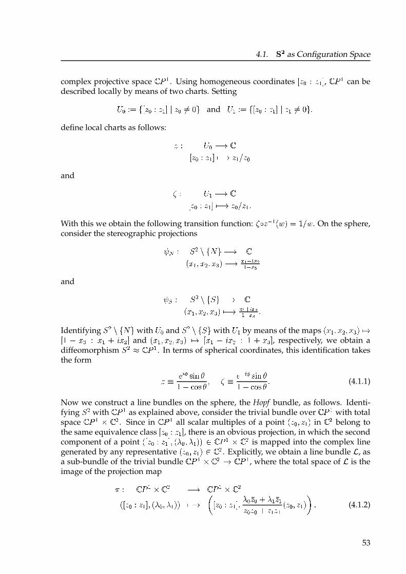
4.1. XY as Configuration Space
complex projective space Z [ \ . Using homogeneous coordinates ]^_ ` ^ \a, Z [ \ can bedescribed locally by means of two charts. Settingb_ `c d ]^_ ` ^ \a e ^_ fc g h and
b \ `c d ]^_ ` ^ \a e ^ \ fc g h idefine local charts as follows: ^ ` b_ jk Z]^_ ` ^ \a ljk ^ \m^_and n ` b \ jk Z]^_ ` ^ \a ljk ^_ m^ \ oWith this we obtain the following transition function:
n p^ q \ rs t c ums . On the sphere,consider the stereographic projectionsv w ` x y z d{ h jk Zr| \ i | y i | } t ljk ~ ���~�\q~�and v � ` x y z dx h jk Zr| \ i | y i | } t ljk ~ ���~�\�~� oIdentifying x y z d{ h with
b_ and x y z dx h withb \ by means of the maps r| \ i | y i | } t lk]u j | } ` | \ � �| y a and r| \ i | y i | } t lk ]| \ j �| y ` u � | } a, respectively, we obtain a
diffeomorphism x y � Z [ \ . In terms of spherical coordinates, this identification takesthe form ^ � ��� ��� �u j �� � � i n � � q�� ��� �u � �� � � o (4.1.1)
Now we construct a line bundles on the sphere, the Hopf bundle, as follows. Identi-fying x y with Z [ \ as explained above, consider the trivial bundle over Z [ \ with totalspace Z [ \ � Z y . Since in Z [ \ all scalar multiples of a point r^_ i ^ \ t in Z y belong tothe same equivalence class ]^_ ` ^ \a, there is an obvious projection, in which the secondcomponent of a point r]^_ ` ^ \a i r�_ i � \ tt � Z [ \ � Z y is mapped into the complex linegenerated by any representative r^_ i ^ \ t � Z y . Explicitly, we obtain a line bundle � , asa sub-bundle of the trivial bundle Z [ \ � Z y k Z [ \ , where the total space of � is theimage of the projection map� ` Z [ \ � Z y jk Z [ \ � Z yr]^_ ` ^ \a i r�_ i � \ tt ljk �]^_ ` ^ \a i �_ �_ � � \ �\^_ �_ � ^ \ �\ r^_ i ^ \ t� o (4.1.2)
53

4. The spin zero case
There is also an inclusion map � � � � � � � � ¡ . The projection and the inclusionmaps induce maps ¢ £ and �£ between the corresponding spaces of sections, so they canbe composed with the trivial connection ¤ ¥¦§ ¨ ©ª « ª ¬
on � � � � ¡ � � � � , in order toobtain a connection on � (the Grassmann connection) by setting ¤ �¨ ©id ¢ £ ¬®¤ ¥¦§ ®�£ .In terms of the local parametrisation � � � � � � ¯ °� ±² � ¯ ³, and of the local section´ ©µ ¬ ¨ ©±² � µ ³ « ©²« µ ¬¬
, the connection takes the following form:¤ ©´ ¬ ¨ ´ ¶ ·ª¯² ¸ ¯ · ¹ º (4.1.3)
The curvature of this connection, written in terms of local coordinates on the sphere, isgiven by [MT97]: » ¼ ¨ ½¾ ¿ÀÁ Â ª Â Ã ª Ä º (4.1.4)
We can use the map ¢ to construct the projector that describes the line bundle � . Letus write Å for ±µÆ � µ �³, the second component of the map ¢ is a map projecting ©Ç¦ « Ç � ¬onto the complex line generated by ©µ¦ « µ � ¬
. At each point Å we can then compute thematrix È ©Å ¬
corresponding to this projection. From the definition of ¢ we have:¶ È �� ©Å ¬ È �¡ ©Å ¬È ¡ � ©Å ¬ È ¡¡ ©Å ¬ ¹ ¶ Ç¦Ç � ¹ ¨ Ǧ ·µ¦ ¸ Ç � ·µ �µ¦ ·µ¦ ¸ µ � ·µ � ¶ µ¦µ � ¹ º (4.1.5)
From this we obtain the following matrix components for È ©Å ¬:È �� ©Å ¬ ¨ µ¦ ·µ¦µ¦ ·µ¦ ¸ µ � ·µ � « È �¡ ©Å ¬ ¨ µ¦ ·µ �µ¦ ·µ¦ ¸ µ � ·µ � «È ¡ � ©Å ¬ ¨ µ � ·µ¦µ¦ ·µ¦ ¸ µ � ·µ � « È ¡¡ ©Å ¬ ¨ µ � ·µ �µ¦ ·µ¦ ¸ µ � ·µ � º
Let us express È ©Å ¬in terms of local coordinates on the sphere. On ɦ we haveµ ©Å ¬ ¨ µ �µ¦ Ê ËÌÍ ¿ÀÁ ² Î ÏÐ ¿  «
so that È �� ©Å ¬ ¨ µ¦ ·µ¦µ¦ ·µ¦ ¸ µ � ·µ �¨ ²² ¸ ÑÒÓÔ Õ¥�Ö×ØÑ Õ §Ô¨ ² ¸ ÏÐ ¿ ¾ «54

4.1. ÙÚ as Configuration SpaceÛ ÜÝ Þß à á âã äâ Üâã äâã å â Ü äâ Üá âãâ Ü ææ å çâã èâ Ü çÝá æ é êëì íîïð ìñò í óæ å Þæ é êëì í àÝìñò Ý í ô õ Üá î õïðö ìñò í ÷
and so on, leading to Û á æö ó æ å êëì í ìñò í î õïðìñò í îïð æ é êëì í ô ø(4.1.6)
Notice that this is a globally well-defined, matrix-valued function on the sphere. Weobtain the same result if we work on the chart ù Ü. There, we haveú Þß à á âãâ Ü û î õïð ìñò íæ å êëì í øThe matrix components obtained are the same. For example,Û ÜÝ Þß à á âã äâ Üâã äâã å â Ü äâ Üá âãâ Ü ææ å çâã èâ Ü çÝá îïð ìñò íæ å êëì í óæ å ìñò Ý íÞæ å êëì í àÝ ô õ Ü
á î õïðö ìñò í øIn terms of the projector Û , the connection takes the form Û ü[GBVF01]. As an explicitcalculation shows, the curvature form trÞÛ üÛ üÛ à coincides with ý þ . It is a well-knownfact that equivalence classes of line bundles over the sphere are in one to one corre-spondence with the integers. The integer labelling a specific line bundle ÿ over thesphere may be obtained by choosing any connection on ÿ and integrating its curvaturetwo-form over the sphere. Up to a factor of
ö� �, this integral is the first Chern number
of the bundle. A projector describing a line bundle on the sphere with Chern numberequal to � is given by Û � á æö ó æ å êëì �í ìñò �í î õïðìñò �í îïð æ é êëì �í ô ø
(4.1.7)
The reader is suggested to look at references [GBVF01], [Pas01] and [Lan01] for furtherconsiderations on this example.
55

4. The spin zero case
4.1.1. Remark. It is interesting to consider the example of the sphere as configurationspace in connection to Dirac’s magnetic monopole. It is well known that the presenceof a magnetic monopole forces the configuration space of an electron to be (effectively)� �
. Dirac’s quantization condition states that the electric and magnetic charges arerelated through �� � � �� , with � integer. In this case, the electron’s wave functionis a section of a line bundle on the sphere, with Chern number �. This fact has manyconsequences, one of them being that a correct definition of angular momentum operatorsrequires a careful consideration of the bundle structure. In fact, although the electron’sspin is being neglected, it turns out that the physically admissible angular momentumoperator can produce a change in sign in the electron’s wave function (when � is odd)or no change at all (when � is even) under a � rotation. The reader is advised to lookat [BL81], p.203, for a physically-motivated discussion of this effect. The relation ofthese angular momentum operators to the lifting of the
� � � � action on the sphere tothe line bundles is made explicit in [GBVF01].
4.1.2. Angular Momentum coupled to a Magnetic Field
Let us now consider an example related to geometric phases. It has been discussed byBerry and Robbins in [RB94] and is relevant for us insofar as it seems to have providedthe motivation for the idea that eventually led these authors to the construction of thespin basis proposed in [BR97]. We will see how bundles the underlying this examplecan also be described in terms of projectors as the one displayed in eq. (4.1.7).
Consider a quantum mechanical system described by the Hamiltonian� � �� � �� (4.1.8)
describing the coupling of a magnetic field �� with an angular momentum �� (electron
or nuclear spin, for instance). For a given value of �� , the eigenvectors of�
can beexpressed in terms of �� � � �
(the eigenvectors of��
and� �
), as follows:�� � � � �� �� �� � � �� � �� � � � �(4.1.9)
where � is determined by the polar angles, � and , of �� :� � �� � �� �!"#$ % �!"#& ' ( (4.1.10)
Suppose that the magnitude of the magnetic field is kept fixed, but different possibleorientations are allowed. In this case, the Hamiltonian above can be seen as dependingon the parameters
�� � �, the parameter space being the sphere. For such a system timeevolution leads to what is known as geometric phase: If the parameters appearing
in the Hamiltonian change) in time describing a loop on parameter space: * +, �� �*�-This change is usually assumed to be adiabatic, but more general situations are also allowed.
56

4.1. ./ as Configuration Space0 12 034 5 12 0644, the original state 78 9 : 0 12 0344;
gains a phase (additional to the usual,dynamical one) which is given by the following expression:<=> ?@A B CD E8 9 : 0 12 0F44 7 GGF 78 9 : 0 12 0F44;H
(4.1.11)
As pointed out in [Sim83], this phase may be understood as the holonomy of a con-nection on a vector bundle which is naturally determined by the parameter-dependentHamiltonian. The Chern number corresponding to this bundle can be shown to beequal to I: .
A description of the bundle, in terms of projectors, can be obtained as follows. For8
fixed, the vectors 78 9 : ; 0@ 78 7 J : J 78 74 form a basis for the representation space K L .On K L , consider the projection M NDOP onto the subspace generated by 78 9 : ;
. Using this,
we can define a family of projections, parametrised by12, namely the projections on
the subspace generated by 78 9 : 0 12 4;:MP Q5 R 0 12 4M NDOP R 0 12 4S T
(4.1.12)
This projector describes a bundle over the sphere (assuming 7 12 7 5 6), with total spaceU0 12 9 1V 4 W X Y Z K L Q MP 0 12 4 1V 5 1V [. In other words, we are considering a bundle over
the parameter space of \ , where the fibers are generated by the (parameter-dependent)eigenvectors of \ . The curvature of the connection MP G, integrated over
X Y, gives us
the Chern number associated to MP :]C 0MP 4 5 6I^ A B_ ` tr0MP GMP GMP 4T
The integral can be evaluated as follows. From the definitions ofR
and MP , we have:GMP 5 A aMP 9 bc dGe f aMP 9 R bgR SdGh TUsing
R SbcR 5 ijk h bc @ klm h bn and taking the cyclicity of the trace into account,one then obtains ]C 0MP 4 5 I: . In the case of the sphere, equivalence classes of linebundles can be labelled by their Chern number, i.e. two line bundles over the sphereare isomorphic if and only if their Chern numbers coincide. Hence we see, from theprevious computation, that MopY q5 r o .
The case: 5 3
is particularly interesting. The curvature of the connection it givesplace to vanishes, implying that there is no geometrical phase arising from closedloops in the parameter space (sphere). However, it turns out that under a cycle go-ing from some point on the sphere to its antipode, the eigenstates change only in asign, which can also be interpreted as a geometrical phase (for a general value of
:,
the states 78 9 : 0@ 12 4;and 78 9 @: 0 12 4;
coincide, up to a phase factor. This implies that78 9 : 5 3 0 12 4;and 78 9 : 5 3 0@ 12 4;
differ by a phase, and it can be shown that the
value of this phase,0@64L , is independent of the paths joining the points
12and @ 12
,tThis path, when projected to uv w , must belong to the non-trivial element of the fundamental group.
57
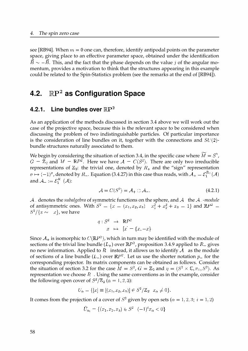
4. The spin zero case
see [RB94]. When x y z one can, therefore, identify antipodal points on the parameterspace, giving place to an effective parameter space, obtained under the identification{| } ~ {|
. This, and the fact that the phase depends on the value � of the angular mo-mentum, provides a motivation to think that the structures appearing in this examplecould be related to the Spin-Statistics problem (see the remarks at the end of [RB94]).
4.2. � �� as Configuration Space
4.2.1. Line bundles over � � �As an application of the methods discussed in section 3.4 above we will work out thecase of the projective space, because this is the relevant space to be considered whendiscussing the problem of two indistinguishable particles. Of particular importanceis the consideration of line bundles on it, together with the connections and � � ���-bundle structures naturally associated to them.
We begin by considering the situation of section 3.4, in the specific case where �� y � � ,� y �� and� y �� � . Here we have � y � �� � �. There are only two irreducible
representations of ��: the trivial one, denoted by �� and the “sign” representation� �� �~��� , denoted by �� . Equation (3.4.27) in this case thus reads, with �� y � ��� �� �and �� y � �¡� �� �: � y � �� � � y �� ¢ � � £ (4.2.1)�� denotes the subalgebra of symmetric functions on the sphere, and �� the ��-moduleof antisymmetric ones. With � � y ¤¥ y �¥ � ¦ ¥� ¦ ¥ § � ¨ ¥ �� © ¥�� © ¥§ y �ª
and � � � y� �«¤¥ } ~¥ ª, we have ¬ � � � � � �¥ �� ¥® y ¤¥ ¦ ~¥ ª
Since �� is isomorphic to � �� � � �, which in turn may be identified with the module ofsections of the trivial line bundle (¯� ) over � � � , proposition 3.4.9 applied to �� givesno new information. Applied to �� instead, it allows us to identify �� as the moduleof sections of a line bundle (¯�) over � � � . Let us use the shorter notation ° � for thecorresponding projector. Its matrix components can be obtained as follows. Considerthe situation of section 3.2 for the case
� y � �, � y �� and ± y �� � ² ³ ¦ ´ � ¦ � � �. Asrepresentation we choose ��. Using the same conventions as in the example, considerthe following open cover of � �«�� (µ y �¦ � ¦ ¶):�· y ¤ ¥® ¸ �¥ � ¦ ¥ � ¦ ¥ § �® ¹ � � «� � ¨ ¥· ºy zª£It comes from the projection of a cover of � � given by open sets (µ y �¦ � ¦ ¶ » ¼ y �¦ �)½�·¾ y ¤�¥ � ¦ ¥ � ¦ ¥ § � ¹ � � ¨ �~ ��¿¥· À zª58

4.2. ÁÂ Ã as Configuration Space
and hence, according to equation (3.2.2), the transition functions for the bundle Ä ÅÆÇare ÈÉ ÊË ÌÍÎ ÏÐ Ñ sgn ÌÎÉ ÐsgnÌÎË ÐÒ (4.2.2)
Note that the right hand side is independent of the choice of representative ÌÎ Ó Ô Î Ç Ô Î Õ Ð ÖÍÎÏ. According to definition 3.2.1, we need a partition of unity, subordinated to thecover ×ØÉ ÙÉ
. Choosing ÚÉ ÌÍÎ ÏÐ Ñ ÛÎÉ Û, we obtain the matrix components of Ü Ý:ÌÜ Ý ÐÉË Þ Á ß Ç à á(4.2.3)ÍÎ Ï âà ÎÉÎË Ò
Note that even though each matrix component of Ü Ý is defined in terms of a represen-tative Î Ö ÍÎÏ, it is an even function on ã Ç
and therefore equivalent to a function onÁ ß Ç.
Remark. We have thus obtained an isomorphism of äå-modules under which the an-tisymmetric functions Î Ó Ô ÎÇ Ô Î Õ Ö ä Ý can be regarded as a set of generators for æ ÌçÝ Ð.Explicitly, we can make the following identification:Îè é êë ÎèÎ ÓÎ èÎÇÎ èÎÕ ìí ÒThus, under this identification, any section of çÝ can be expressed as a linear combi-nation of the form î ÓÎ Ó ï îÇÎÇ ï îÕÎÕ , with îè Ö äå . The (module) multiplication ofthe function îè (regarded as element of ð ÌÁ ß Ç Ð) and Îè (regarded as a section of çÝ) isimplemented in the isomorphic image of æ ÌçÝ Ð inside ä by the usual multiplication offunctions on ã Ç
.
Some of the properties of Ü Ý are:ñ The line bundle çÝ represented by the projector Ü Ý is not trivial. This can be seenas follows: the isomorphisms æ Ìç Ý Ð ò Ü Ý Ìä Õå Ð ò ä Ý allow us to represent everysection as an antisymmetric function on the sphere. One can then use the factthat every such function vanishes at some point to show that we cannot find anowhere vanishing section of çÝ.ñ The connection naturally associated to this bundle is defined as ó Ñ Ü Ý ô. Adirect calculation shows that it has vanishing curvature, i.e., it is a flat connection.Its action on an arbitrary section can be found, using the Leibniz rule, once weknow its action on the set ×Îè Ùè of generators. By direct computation we find:Ü Ýô êë ÎèÎ ÓÎ èÎÇÎ èÎÕ ìí Ñ êë ÎÇÓ Î ÓÎÇ Î ÓÎÕÎ ÓÎÇ ÎÇÇ ÎÇÎÕÎ ÓÎÕ ÎÇÎÕ ÎÇÕ ìí êë ô ÌÎèÎ Ó Ðô ÌÎ èÎÇ Ðô ÌÎ èÎÕ Ð ìíÑ õö êë Îö Î ÓÎö ÎÇÎö ÎÕ ìí ô ÌÎèÎö Ð Ô
59
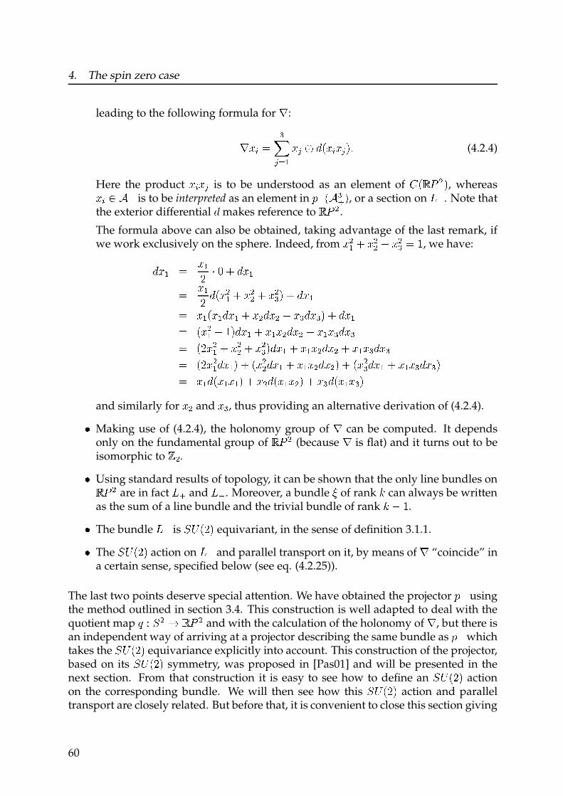
4. The spin zero case
leading to the following formula for ÷ :÷øù ú ûüýþÿ øý � � �øùøý � � (4.2.4)
Here the product øùøý is to be understood as an element of � �� � � �, whereasøù � is to be interpreted as an element in � � � û �, or a section on ��. Note thatthe exterior differential � makes reference to
� � �.
The formula above can also be obtained, taking advantage of the last remark, ifwe work exclusively on the sphere. Indeed, from ø �ÿ � ø �� � ø �û ú �, we have:�ø ÿ ú ø ÿ� � � � �ø ÿú ø ÿ� � �ø �ÿ � ø �� � ø �û � � �ø ÿú ø ÿ �ø ÿ�ø ÿ � ø � �ø � � øû�øû � � �ø ÿú �ø �ÿ � ���ø ÿ � ø ÿø � �ø � � ø ÿøû�øûú ��ø �ÿ � ø �� � ø �û ��ø ÿ � ø ÿø � �ø � � ø ÿøû�øûú ��ø �ÿ�ø ÿ � � �ø �� �ø ÿ � ø ÿø ��ø � � � �ø �û�ø ÿ � ø ÿøû�øû �ú ø ÿ� �ø ÿø ÿ � � ø � � �ø ÿø � � � øû� �ø ÿøû �and similarly for ø � and øû , thus providing an alternative derivation of (4.2.4).� Making use of (4.2.4), the holonomy group of ÷ can be computed. It dependsonly on the fundamental group of
� � �(because ÷ is flat) and it turns out to be
isomorphic to ��.� Using standard results of topology, it can be shown that the only line bundles on� � �are in fact � and �� . Moreover, a bundle � of rank � can always be written
as the sum of a line bundle and the trivial bundle of rank � � �.� The bundle �� is � � ��� equivariant, in the sense of definition 3.1.1.� The � � ��� action on �� and parallel transport on it, by means of ÷ “coincide” ina certain sense, specified below (see eq. (4.2.25)).
The last two points deserve special attention. We have obtained the projector � � usingthe method outlined in section 3.4. This construction is well adapted to deal with thequotient map � � � � � � � �
and with the calculation of the holonomy of ÷ , but there isan independent way of arriving at a projector describing the same bundle as � � whichtakes the � � ��� equivariance explicitly into account. This construction of the projector,based on its � � ��� symmetry, was proposed in [Pas01] and will be presented in thenext section. From that construction it is easy to see how to define an � � ��� actionon the corresponding bundle. We will then see how this � � ��� action and paralleltransport are closely related. But before that, it is convenient to close this section giving
60

4.2. �� as Configuration Space
yet another description of the non-trivial line bundle !" over the projective space, interms of local trivialisations (this will be used when we compare parallel transportwith the # $ %&' action, in the next section).
We will denote points on the sphere by ( ) %( * + (, + ( - '. Under the quotient map . ,( goes to an equivalence class /( 0 ) 1( + 2( 3, representing a point in � 4 ,. Using ho-
mogeneous coordinates, /( 0 can equivalently be described as the line generated by ( ,regarded as a vector in � -
: /( 0 ) 15( 65 7 � 38An open cover of the projective plane is given by$9 ) 1 /(0 6 ( 9 :) ;3+ %< ) =+ & + > '8The corresponding local charts 1%$9 + ?9 '39 are given by?* @ $ * 2A � ,/(0 B2A C(,( * + (-( * D (4.2.5)
and analogously for ?, and ?-. The bundle !" can be constructed as a sub-bundle ofthe trivial bundle � 4 , E F -
. The explicit construction goes as follows. First, the totalspace G %!" ' of the bundle is defined, as a set, in the following way:G %!" ' @) 1%/( 0 + 5 6H %( 'I' 7 � 4 , E F - 6 5 7 F + ( 7 /(0 3 + (4.2.6)
where 6H %( 'I ) %( * + (, + ( - ' 8 (4.2.7)
Note that there is some ambiguity in the description of the elements of G %!" ', namely,the choice of 5 is not unique, since we are using a representative ( of /( 0 in the argumentof 6H %2'I which of course is a well defined function only over the sphere , not over theprojective plane. But in view of the relation 6H %2( 'I ) 2 6H %( 'I (that is also satisfied by6J I), we may describe an element K 7 G %!" ' in (exactly) two ways:K ) %/(0 + 5 6H %( 'I' ) %/( 0 + %25' 6H %2( 'I'8Notice that the same situation is faced in the construction of tautological bundles overprojective spaces (see for example [MS74]) .G %!" ' is given the relative topology with respect to the product space � 4 , E F -
. Theprojection map is obviously defined asL %/( 0 + 5 6H %( 'I' @) /(0 8Local trivialisations can then be defined through %< ) =+ & + > ':M9 @ L "* %$9 ' 2A $9 E F%/( 0 + 5 6H %( 'I' B2A %/(0 + sgn %( 9 '5 '8 (4.2.8)
61
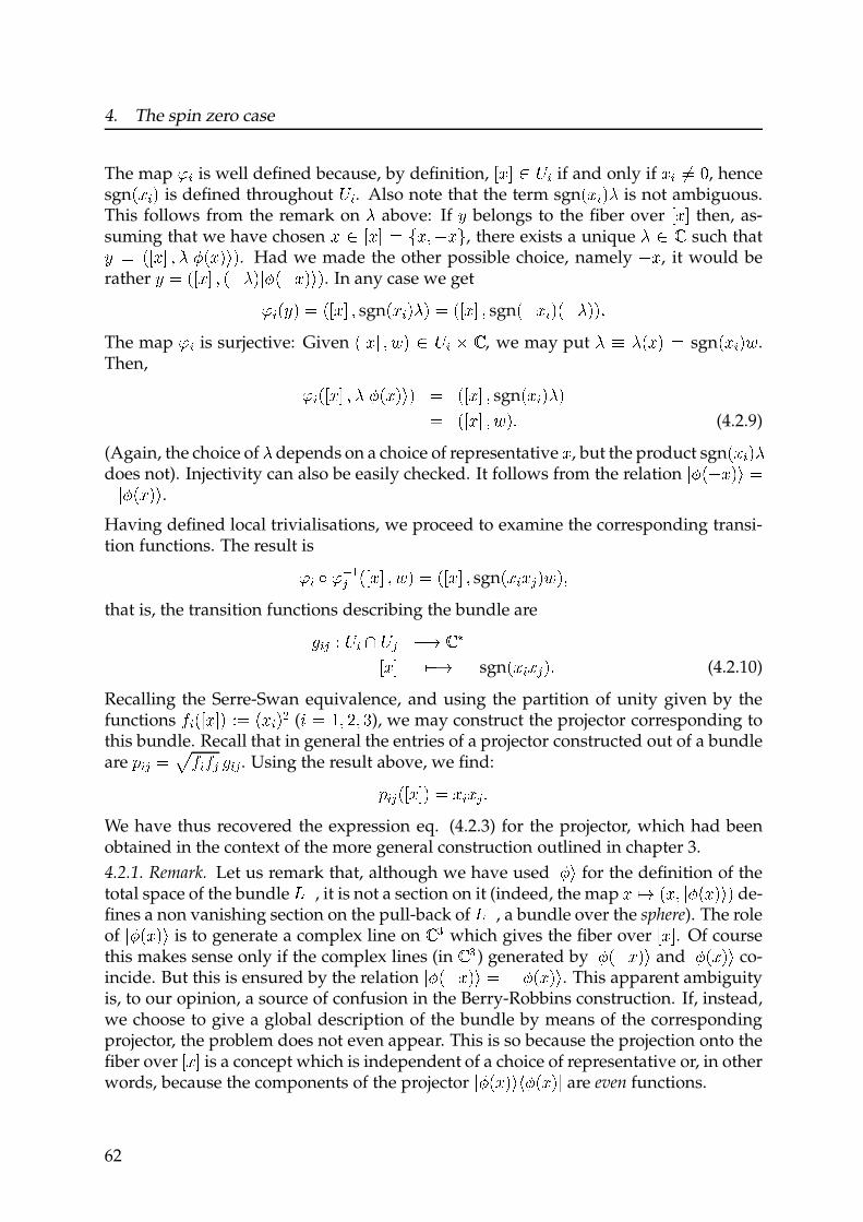
4. The spin zero case
The map NO is well defined because, by definition, PQ R S TO if and only if QO UV W, hencesgn XQ O Y is defined throughout TO. Also note that the term sgnXQ O YZ is not ambiguous.This follows from the remark on Z above: If [ belongs to the fiber over PQ R then, as-suming that we have chosen Q S PQR V \Q ] ^Q _, there exists a unique Z S ` such that[ V XPQR ] Z ab XQ YcY. Had we made the other possible choice, namely ^Q , it would berather [ V XPQR ] X^ZY ab X^Q YcY. In any case we getNO X[ Y V XPQ R ] sgnXQ O YZ Y V XPQR ] sgnX^QO YX^ZYYdThe map NO is surjective: Given XPQ R ] e Y S TO f ` , we may put Z g Z XQ Y V sgn XQ O Ye .Then, NO XPQ R ] Z ab XQ YcY V XPQ R ] sgnXQ O YZ YV XPQR ] e Yd (4.2.9)
(Again, the choice of Z depends on a choice of representative Q, but the product sgnXQ O YZdoes not). Injectivity can also be easily checked. It follows from the relation ab X^Q Yc V^ ab XQ Yc.Having defined local trivialisations, we proceed to examine the corresponding transi-tion functions. The result isNO h Nijk XPQ R ] e Y V XPQR ] sgnXQ OQk Ye Y]that is, the transition functions describing the bundle arelOk m TO n Tk ^o ` pPQR q^o
sgn XQ OQk Yd (4.2.10)
Recalling the Serre-Swan equivalence, and using the partition of unity given by thefunctions rO XPQ R Y mV XQO Ys (t V u] v ] w), we may construct the projector corresponding tothis bundle. Recall that in general the entries of a projector constructed out of a bundleare x Ok V yrOrk lOk . Using the result above, we find:x Ok XPQ RY V QOQk dWe have thus recovered the expression eq. (4.2.3) for the projector, which had beenobtained in the context of the more general construction outlined in chapter 3.
4.2.1. Remark. Let us remark that, although we have used abc for the definition of thetotal space of the bundle zi , it is not a section on it (indeed, the map Q qo XQ ] ab XQ YcY de-fines a non vanishing section on the pull-back of zi, a bundle over the sphere). The roleof ab XQ Yc is to generate a complex line on ` { which gives the fiber over PQ R. Of coursethis makes sense only if the complex lines (in ` { ) generated by ab X^Q Yc and ab XQ Yc co-incide. But this is ensured by the relation ab X^Q Yc V ^ ab XQ Yc. This apparent ambiguityis, to our opinion, a source of confusion in the Berry-Robbins construction. If, instead,we choose to give a global description of the bundle by means of the correspondingprojector, the problem does not even appear. This is so because the projection onto thefiber over PQ R is a concept which is independent of a choice of representative or, in otherwords, because the components of the projector ab XQ Yc |b XQ Y a are even functions.
62

4.2. }~ � as Configuration Space
Now we consider local frames and parallel transport. Let us define�� � } � � �� � ��� ��� � ��� ���� � � � �� �� ����(4.2.11)
These global sections vanish at some points, so they can only give place to local frames,given by their restrictions to the respective neighborhoods ��. Since the connection weconsider on
��is flat, the result of parallel transport can only depend on the homo-
topy type of the chosen path. For our purposes, it will be enough to consider paralleltransport along the following path�:� � ��� �� � � ��� �� �� � } � �� ��� � � �� �� � � ¡ � ¢£� �� � � � (4.2.12)
On �� , any section can be written in terms of �� . The action of the connection ¤(eq.(4.2.4)) on it is ¤�� ¥ �¦ § ¨© ¦ ª �� § ¨©� ª �� § ¨©� �where ©� ��� � � ¥ ���� . From
�© ¦ �� �� ��« ¥ ¢£�� � � �� � �,�©� �� �� ��« ¥ ¡ and
�©� �� �� ��« ¥�� ¢£� � �� �(note that in these expressions there is no dependence on the choice of
representatives) we obtain, using the fact that ¢£� � ¬¥ ¡ on the interval considered:¤ ® ¯°±�� �� � ¥ �¢£�� � � �� � � � � ¦ �� � � �� ¢£� � �� � � �� �� �¥ � ²³ � �� �� � � (4.2.13)
To find a parallel section along � , we must solve the equation¨´� �� �� � ª ´ �� �¤ ® ¯°±�� �� � ¥ ¡ �The solution is given by ´ ��� ¥ �¢£� � ��¦
, so thatµ � ��� �� � � ��� �� � ��� �� ��� �� �� � � ��� � � ¡ � ¢£� � ��(4.2.14)
is a parallel section along � .
4.2.2. ¶· ¸¹º equivariance
The sphere, being a homogeneous space for » � ��� (» � ¼¥ » � ����� �½�) carries a natural» � ���-action » � ��� ¾ » � �� » � �¿
The reason for this choice of path is that it can be obtained from the action of À Á ÂÃÄ on ÅÆ Ç .
63
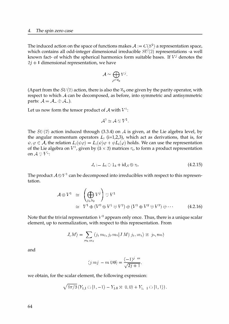
4. The spin zero case
The induced action on the space of functions makes È ÉÊ Ë ÌÍ Î Ï a representation space,which contains all odd-integer dimensional irreducible Í Ð ÌÑÏ representations -a wellknown fact- of which the spherical harmonics form suitable bases. If Ò Ó denotes theÑÔ Õ Ö dimensional representation, we haveÈ × ØÓ ÙÚÛ Ò Ó Ü(Apart from the Í Ð ÌÑÏ action, there is also the ÝÎ one given by the parity operator, withrespect to which È can be decomposed, as before, into symmetric and antisymmetricparts: È Ê ÈÞ ß È à).
Let us now form the tensor product of È with Ò á:Èâ × È ã Ò á ÜThe Í Ð ÌÑÏ action induced through (3.3.4) on È is given, at the Lie algebra level, bythe angular momentum operators äå (i=1,2,3), which act as derivations, that is, foræ ç è é È , the relation äå Ìæ èÏ Ê äå Ìæ Ïè Õ æäå Ìè Ï holds. We can use the representationof the Lie algebra on Ò á, given by (ê ë ê) matrices ìå , to form a product representationon È ã Ò á: íå ÉÊ äå ã Öâ Õ idî ã ìå Ü (4.2.15)
The product È ã Ò á can be decomposed into irreducibles with respect to this represen-tation. È ã Ò á × ïØÓ ÙÚÛ Ò Ó ð ã Ò á× Ò á ß ÌÒ ñ ß Ò á ß Ò Î Ï ß ÌÒ á ß Ò Î ß Ò â Ï ß ò ò ò (4.2.16)
Note that the trivial representation Ò ñ appears only once. Thus, there is a unique scalarelement, up to normalization, with respect to this representation. Fromóíç ô õ Ê ö÷ ø ù÷ ú ÌÔ á û á ç Ô Î û Î óí ô Ï óÔ á ç û áõ ã óÔ Î ç û Î õand ÌÔ ûÔ ü û óý ýÏ Ê ÌüÖÏÓ à÷þÑÔ Õ Ö çwe obtain, for the scalar element, the following expression:ÿ�� �ê Ì� áùá ã óÖç üÖõ ü � áùñ ã óý ç ýõ Õ � áùàá ã óÖç ÖõÏ Ü64

4.2. �� � as Configuration Space
Identifying �� with � �, this is the same as� � �� � ��� �� ������� ���� ����� � ��� � !"#$ %&' (� )*% (� �!"#$ %&' ( �+� , (4.2.17)
One checks readily that� �
is indeed a scalar element, that is that -. � � � /holds.
In terms of the group representation, this means that 0 1�2 34 5 � 34 ��6 5� � � 36 5� or,equivalently, that 0 1�2 34 5 � 36 5� � � 346 5� , (4.2.18)
This property of� �
will be used below in order to construct an 7 8 395 bundle structureon the line bundle it gives place to. As an � -valued vector,
� �has remarkable prop-
erties. One of them is that it provides the construction we are looking for, namely, wehave the following result.
4.2.2. Proposition (cf.[Pas01]). Define a projector on �� by : �� � � ; �, Then, the followingisomorphism of �< modules holds: : 3� �< 5 = � � , (4.2.19)
Proof. First of all, let us note that the spherical harmonics >� ��� ? � ��� ? � ����@ are a set ofgenerators of �� over �< . Written in matrix form, the projector is given by
: � ����� �� � A BCBD �$ �� �A BC�D �$ ��� �A EC�D �$ ��$A BC�D �$ �� �� F A �GCBD �$ �� A BC�D �$ ����A EC�D �$ �$ �A BC�D �$ �� �� � A BCBD �$ ���+++� , (4.2.20)
Denote with H< ? H� and H� the three columns of : in (4.2.20). They are a set of generatorsof the module : 3� �< 5, since every element I on it is of the formI � JH< F KH� F LH� ?with
J ? K and L in �< . Therefore, we define the map M � : 3� �< 5 N � � as the �<-linearextension of M 3HO 5 �� � ��O (4.2.21)M 3H� 5 �� � ��� ,The generators >H. @. are not independent over �< , there are relations among them, of
65

4. The spin zero case
the form PQ RSTQ U VQ T WXQ Y Z. They can be read off from (4.2.20):[\] ^ _ `a`b cd efg Xh U _ `aib cd ej Xf ^ _ kaib cd ed Xl Y Z m_ `aib cd elj Xh ^ [\] U _ ina`b cd efg Xf ^ _ `aib cd ej Xl Y Z m_ kaib cd eld Xh U _ `aib cd elj Xf ^ [\] U _ `a`b cd efg Xl Y Z oA direct calculation shows that these relations are also satisfied by the generators ofpl. This completes the proof and establishes an equivalence of modules between Vand V l.
We have seen several ways in which ql and its module of sections can be described.Using the method described in chapter 3, we have obtained r Rql W sY V l Rp th W, withV l Y uvw xv u and
vgiven by eq. (4.2.7). From 4.2.2 it follows that r Rql W sY V yp th W, withV z u{ w x{ u and
{given by eq. (4.2.17). We have, therefore,V l Rp th W sY p l sY V yp th Wo (4.2.22)
The description of the total space of ql using eq. (4.2.6) has been used in order to find aparallel section along the section | . From that calculation one sees that if | is extendedto a closed loop, the holonomy corresponding to that loop is Ui
. We will now considerthe } ~ R\W equivariance of ql and we will compare it with parallel transport. For thatpurpose, let us consider an alternative description of the total space of ql , obtained byusing u{ w
in eq. (4.2.6) instead of uvw. This implies that the open cover and transitionfunctions will be different, but, because of eq. (4.2.22), they give place to isomorphicbundles. The advantage of this particular construction of the bundle lies in the fact thatu{ w
is invariant under } ~ R\W. Equation (4.2.18), which we write again below, expressesthis fact in a convenient way: � yj� R� W u{ R� Ww Y u{ R�� Ww o (4.2.23)
Since u{ R� Ww R Y U u{ RU� Ww W spans the fiber over �� �, we see that the action of an element� � } ~ R\W on � Y R��� m �{ R� WW � a lj R�� �W can be correctly defined by setting�� R� W �Y R���� m �� yj� R� W u{ R� WWw (4.2.24)Y R���� m � u{ R�� WwWoIn fact, from the last expression we see explicitly that � is mapped into the correct fiber:�� R� W � a lj R� � �� �W. From this and the fact that we are using a representation of } ~ R\Wfor its definition, the map � fulfills the conditions stated in definition (3.1.1), givingplace to an } ~ R\W-bundle structure on ql.
66

4.2. �� � as Configuration Space
In order to compare parallel transport with the � � ��� action just defined, we use(4.2.24) to find the explicit form of the action on ��, when described in terms of ���.First let us note that, for all � , we have �� �� �� � � �� �� ��, where � is a unitary matrix(with constant entries). Hence, we may replace
�by
�in (4.2.24), provided we also
replace � ��� � � by � ¡� ��� � �� . For ¢ � � ��� written in matrix form as � £ ¤ ¥¦ §¥ §¤ ¨we have, for the 3-dimensional representation,� ��� � � � ©ª ¤« ¬�¤¥ ¥ «¦¬�¤ §¥ � �¤ �« ¦ �¥ �« � ¬� §¤¥§¥ « ¦¬� §¤ §¥ §¤« ® ¯This leads to
� ¡ � ��� � � � � ©°°°°ª �« �¤« ¦ ¥ « ¦ §¥ « ± §¤« � ¦ ²« �¤« ± ¥ « ¦ §¥ « ¦ §¤« � ¦ �¤¥ ± §¤ §¥ �²« �¤« ± §¥ « ¦ ¥ « ¦ §¤« � �« �¤« ± ¥ « ± §¥ « ± §¤« � ¦³ �¤¥ ¦ §¤ §¥ ��« �¤ §¥ ± §¤¥ � ¦ ²« �¤ §¥ ¦ §¤¥ � ��¤ �« ¦ �¥ �« � ® ¯The path µ �¶ � � ·�¸¹º ¶ » ¼ » ½¾¸ ¶ �¿ may be obtained from the � � ��� action on � À « . In fact,with �Á � �¼ » ¼ » Â� and à � Ä ½¾¸ ë ¦ ¸¹º 븹º ë ½¾¸ ë Å »one gets µ �¶ � � Ã Æ ·� Á ¿. Now, since �·� Á ¿ » �¼ » ¼ » Â�� lies in the fiber over
·� Á ¿, we mayconsider its image under the action of Ã:ÇÈÉ �·� Á ¿ » �¼ » ¼ » Â�� � Ê Ã Æ ·� Á ¿ » � ¡ � ��� � à �� �¼ » ¼ » Â�à Ë� �µ �¶ �» �¸¹º ¶ » ¼ » ½¾¸ ¶ ���Ì Í« Í�Ì �� Î �¶ � ¯ (4.2.25)
4.2.3. Two Identical Particles of Spin Zero
As remarked in the introduction, the classical configuration space of a system of Ïidentical particles moving in � Ð is defined the quotient space, ÑÒ � ÓÑÒ Ô�Ò , obtainedfrom the natural action of the permutation group �Ò on the spaceÓÑÒ � Õ�Ö � » ¯ ¯ ¯ » ÖÒ � ¢ � ÐÒ � Ö² ×� ÖØ for all pairs�³ » Ù �Ú ¯This is a multiply-connected space and so, according to the general considerations pre-sented in chapter 2, and following [LM77], we consider wave functions to be given bysquare integrable sections of some vector bundle on ÑÒ .
67
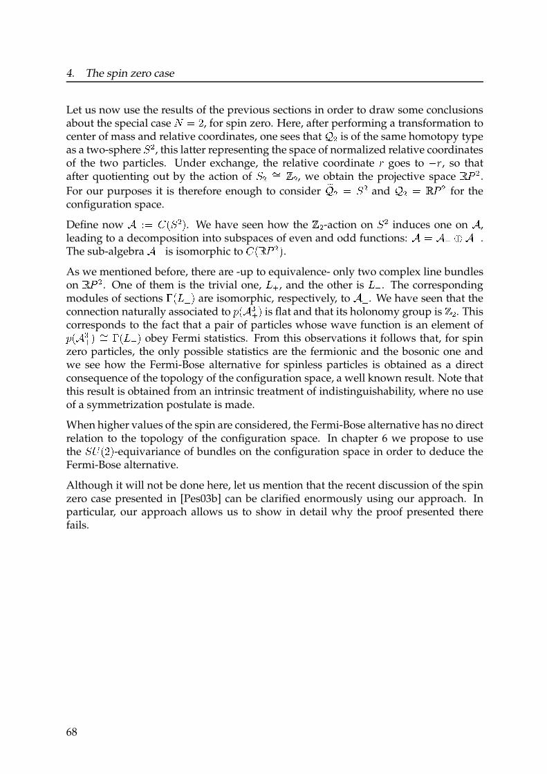
4. The spin zero case
Let us now use the results of the previous sections in order to draw some conclusionsabout the special case Û Ü Ý, for spin zero. Here, after performing a transformation tocenter of mass and relative coordinates, one sees that Þß is of the same homotopy typeas a two-sphere à ß
, this latter representing the space of normalized relative coordinatesof the two particles. Under exchange, the relative coordinate á goes to âá , so thatafter quotienting out by the action of àß ãÜ äß, we obtain the projective space å æ ß
.
For our purposes it is therefore enough to consider çÞß Ü à ßand Þß Ü å æ ß
for theconfiguration space.
Define now è éÜ ê ëà ß ì. We have seen how the äß-action on à ß
induces one on è ,leading to a decomposition into subspaces of even and odd functions: è Ü èí î è ï .The sub-algebra èí is isomorphic to ê ëå æ ß ì
.
As we mentioned before, there are -up to equivalence- only two complex line bundleson å æ ß
. One of them is the trivial one, ðí , and the other is ðï. The correspondingmodules of sections ñ ëðò ì
are isomorphic, respectively, to èò . We have seen that theconnection naturally associated to ó ëè ôí ì
is flat and that its holonomy group is äß. Thiscorresponds to the fact that a pair of particles whose wave function is an element ofó ëè ôí ì ãÜ ñ ëðï ì obey Fermi statistics. From this observations it follows that, for spinzero particles, the only possible statistics are the fermionic and the bosonic one andwe see how the Fermi-Bose alternative for spinless particles is obtained as a directconsequence of the topology of the configuration space, a well known result. Note thatthis result is obtained from an intrinsic treatment of indistinguishability, where no useof a symmetrization postulate is made.
When higher values of the spin are considered, the Fermi-Bose alternative has no directrelation to the topology of the configuration space. In chapter 6 we propose to usethe à õ ëÝì-equivariance of bundles on the configuration space in order to deduce theFermi-Bose alternative.
Although it will not be done here, let us mention that the recent discussion of the spinzero case presented in [Pes03b] can be clarified enormously using our approach. Inparticular, our approach allows us to show in detail why the proof presented therefails.
68
5. Applications to the Berry-Robbins
approach to Spin-Statistics
We have remarked in the previous chapters that one of the motivations in the searchfor a geometric proof of the Spin-Statistics theorem is the fact that, for identical spin-less particles, the Fermi-Bose alternative follows as a consequences of the non-trivialtopology of the configuration space. The possibility of a geometric origin of the Spin-Statistics relation was already proposed by Leinaas and Myrheim [LM77] and has beena subject of interest for many years. But there is a big obstacle in the way to eventu-ally achieving such a goal: The results in the motivational case (i.e. the example ofquantum mechanics of identical spinless particles) are obtained within a framework inwhich quantization ideas play a key role. It is more than questionable that a methodbased on a quantization scheme may also be applied when electron spin (which hasno classical analogö) is considered. A reasonable way out of this difficulty is to adopta compromise position, by adding “by hand” the structures needed to describe spinto the ones that have already been obtained for the zero spin case by a well foundedquantization algorithm. Such a strategy necessarily involves a certain amount of trialand error and it is for this reason that the implementation of different constructionsand a comparison between them is welcome, since this might provide some insightinto the problem.
Among these constructions are the one proposed by Berry and Robbins [BR97], aswell as further developments of it [BR00, HR04]. The original construction attemptsto tackle the issue of indistinguishability, making use of a certain single-valuednessrequirement on the wave function, in the hope that a derivation of the Spin-Statisticstheorem will be achieved. It has the virtue of being concrete and of reproducing thecorrect relation between Spin and Statistics for all values of the spin but, this one notbeing the only construction satisfying their assumptions (see [BR00]), the derived Spin-Statistics relation gets lost. Anyway, the Berry-Robbins approach leaves, in our opin-ion, many open questions, and the formalism used does not very easily allow to isolatetechnical aspects from physical ones. It is therefore of interest to have a new look atthese constructions from a different point of view. This is what is done in this chapter,where the tools developed in chapter 3 are used to reproduce and, most importantly,to interpret the Berry-Robbins construction. Our method will allow us to show that the÷
See, however, [BH50].
69
5. Applications to the Berry-Robbins approach to Spin-Statistics
single-valuedness condition of Berry and Robbins is not consistent.
5.1. Review of the construction
We begin with a review of the construction presented in [BR97], which is restricted tothe two particle case. Recall that for two identical particles moving in three spatial di-
mensions the configuration space, ø, is obtained from ùø ú ûüýþ ÿ ý� � � � � � � � � ý þ �ú ý� �by identifying exchanged configurations: üý ÿ ý � üý ÿ ý �
. The resulting space, ø úùø� , is homotopy equivalent to the projective plane
� � �. This is easily seen by per-
forming, in ùø, the change of coordinates üý þ ÿ ý� � � ü� ÿ ý �, where � is the center of
mass position vector, and ý the relative position vector. From this we see that ùø splitsas the product
� � � � � � � �. Under exchange, all points of the first two factors (that
are contractible) remain unchanged, whereas points in the sphere are mapped to theirantipodes. Identification of antipodes in the sphere gives place to a projective plane,
so we might as well set ùø ú � �and ø ú � � �
.
The spin degrees of freedom are introduced in the formalism in the following way. In apreliminary step, consider the usual description by means of states of the form
�� ÿ � þ� ��� ÿ � ��. Following [BR97], let us introduce the notation�� � for these states, where
the index “�
” refers to the ordered pair of quantum numbers û� þ ÿ � � � (the quantumnumber � will be implicitly understood from now on). For the pair û� � ÿ � þ�, whichelements were permuted, the index “
�” will be used�. Now, the spin basis û �� ���
will be replaced by a “transported” one, that depends on the positions: û �� üý ���� ÿ ý �ù� .
In order to obtain the transported basis from the fixed one, a position-dependent uni-tary operator � üý �
is introduced. The idea is to construct � üý �in such a way that a con-
tinuous exchange of the particles’ positions is accompanied by a (continuous, as well)exchange of spin labels. This will require the embedding of the fixed basis û �� ��� ina larger vector space, that will be denoted with � . Schwinger’s representation of spinin terms of creation and annihilation operators proves to be particularly useful for theconstruction of an operator � üý �
with the required properties. Let us explain why.
In the Schwinger representation, the spin operators (for one particle states) are con-structed with the help of operators � ��� ÿ � ��� satisfying the commutation relations
� ÿ ��! ú " � ÿ �� ! ú "#$In other words: if %& ' ( %) * + ,' - %) * + . '
, then %& ' ( %) * + . ' - %) * + ,' /70

5.1. Review of the construction
One then defines the spin operators as follows:0 1 23 45 6789 : 987 ;0< 23 =5 6987 > 789; (5.1.1)0? 23 45 6787 > 989; @The commutation relations A0B C 0D E 3 =FBD G 0G
hold, so these operators provide a repre-sentation of HI 65;. Common eigenvectors of J<
and0?
are given byKL C M NO 23 678 ;NPQ R 698 ;NSQ RT 6L : M N ;U6L > M N ;U KVO @ (5.1.2)
If we denote with WX 6WY ; the exponent of 78 698 ; in equation (5.1.2), then we can writethe quantum numbers L and
M Nin the following form:L 3 45 6WX : WY ; M N 3 45 6WX > WY ;@ (5.1.3)
From this expression, one sees that a change in the sign of the quantum numberM N
,due to a rotation by an angle of Z in which [\?
goes to > [\?, can also be effected by
exchanging 78 with 98. Now, since in order to describe the spin states of two particlesmore operators are needed (say 7 1 C 9 1 C 7< C 9<
, plus the corresponding creation operators),one might ask: What meaning do the different possible exchanges of operators have,in terms of rotations? For, whereas the relation between the exchange 7B ] 9B
and the
change in sign ofM ^_`N
under a Z rotation is clear from the expression0 ^_`? 3 4a5 678B 7B >98B 9B ; for the third component of the spin operator of particle =, exchanges of the form7 b8c1 ] 7 b8c<
or 9 b8c1 ] 9b8c<should be related, respectively, to operators of the form d Xe? 3
4a5 67 817 1 > 78<7< ; or dYe? 3 4a5 69819 1 > 98< 9< ; and so on, which do not have an immediateinterpretation in terms of rotations. The complete set of operators related to this typeof exchange (4 ] 5
) is, according to equation (5.1.1),
d Xe1 23 45 67817< : 78<7 1 ;C d Y e1 23 45 69819< : 98< 91 ; CdX e< 23 =5 678<7 1 > 7817< ;C d Y e< 23 =5 698< 9 1 > 9819< ; C
(5.1.4)
dX e? 23 45 67817 1 > 78<7< ;C d Y e? 23 45 69819 1 > 98< 9< ; @One checks readily that they satisfy the same commutation relations as the spin op-erators ( Ad X bYc eB C d X bYc eD E 3 =FBD G d X bYc eG ) and hence provide yet another representation ofHI 65;. Since the 7-operators commute with the 9-ones, this is still true for f 23 fg : f h(where f g bh c 23 6dX bYc e1 C dX bYce< C d X bYc e? ;). Exponentiating it, we obtain a representationij 2 0 k 65; l Gl6m ;, where m is the space generated by the basisKW 1X C W<X C W 1Y C W<Y O 3 6781 ;n op 678< ;nqp 6981 ;n or 698< ;n qrT 6W 1X ; U6W<X ; U6W 1Y ; U6W<Y ; U KVO @ (5.1.5)
71
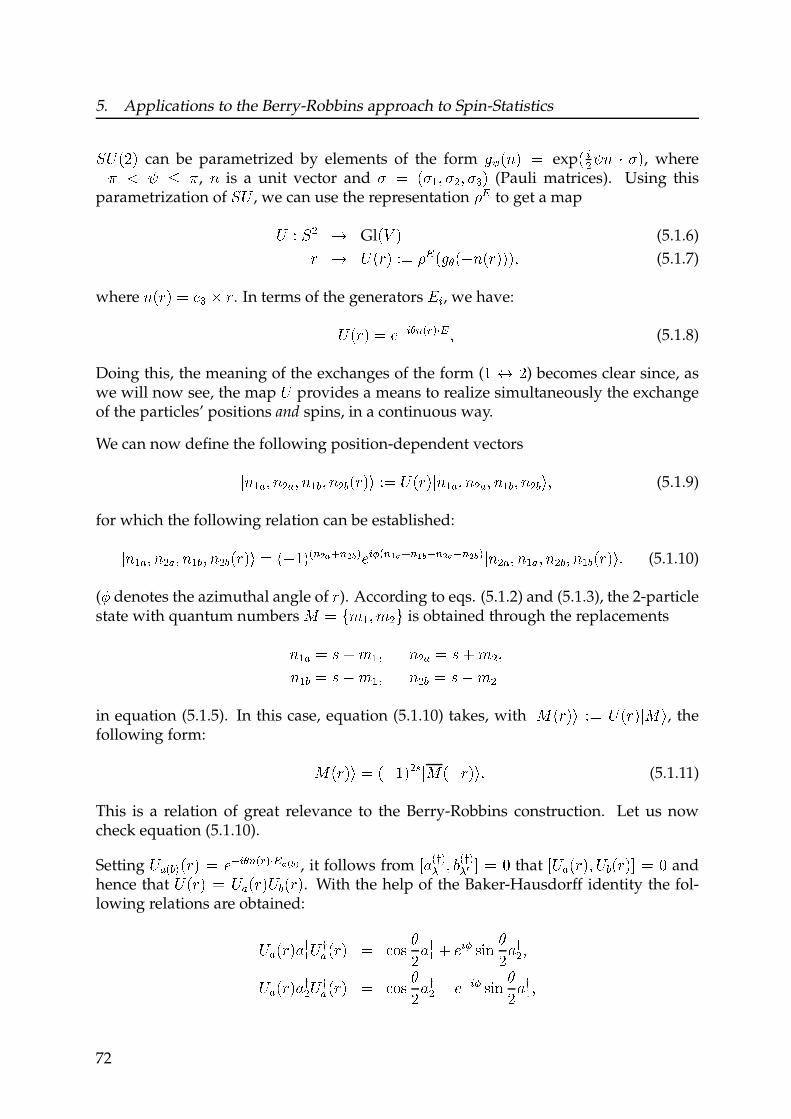
5. Applications to the Berry-Robbins approach to Spin-Statistics
s t uvwcan be parametrized by elements of the form xy uz w {
expu |} ~ z � � w
, where�� � ~ � � ,z
is a unit vector and� { u� � � �} � �� w
(Pauli matrices). Using thisparametrization of
s t, we can use the representation �� to get a mapt � s } �
Glu� w
(5.1.6)� � t u� w �{ �� ux� u�z u� www �(5.1.7)
wherez u� w { �� � � . In terms of the generators �|, we have:t u� w { ��|�� �� � �� �
(5.1.8)
Doing this, the meaning of the exchanges of the form (� � v) becomes clear since, as
we will now see, the mapt
provides a means to realize simultaneously the exchangeof the particles’ positions and spins, in a continuous way.
We can now define the following position-dependent vectors�z �� � z}� � z �� � z }� u� w� �{ t u� w �z �� � z}� � z �� � z }� � �(5.1.9)
for which the following relation can be established:�z �� � z}� � z �� � z }� u� w� { u� �w���� ��¡ ��|¢ �� £� � £¡ �� �� ���¡ � �z }� � z �� � z}� � z �� u� w� ¤(5.1.10)
(¥ denotes the azimuthal angle of �). According to eqs. (5.1.2) and (5.1.3), the 2-particlestate with quantum numbers ¦ { §¨ � � ¨ } © is obtained through the replacementsz �� { ª « ¨ � � z}� { ª « ¨ } �z �� { ª � ¨ � � z}� { ª � ¨ }in equation (5.1.5). In this case, equation (5.1.10) takes, with
�¦ u� w� �{ t u� w �¦ �, the
following form: �¦ u� w� { u� �w}¬ �¦ u�� w� ¤(5.1.11)
This is a relation of great relevance to the Berry-Robbins construction. Let us nowcheck equation (5.1.10).
Settingt���� u� w { ��|�� �� � ��� ¡® , it follows from ¯° �±�² � ³ �±�²´ µ { ¶
that ¯t� u� w� t� u� wµ { ¶and
hence thatt u� w { t� u� wt� u� w
. With the help of the Baker-Hausdorff identity the fol-lowing relations are obtained:
t� u� w°±�t ±� u� w { ·¸¹ ºv °±� « �|¢ ¹»¼ ºv °±} �t� u� w°±} t ±� u� w { ·¸¹ ºv °±} � ��|¢ ¹»¼ ºv °±� �
72

5.1. Review of the construction
and analogously for ½¾¿ . From this one then obtains:À Á ÃÁľŠÃÆ ÇÈ ÁÄ¾É ÃÆ ÊÈ Á½¾Å ÃÆ ÇË Á½¾É ÃÆ ÊË ÌÍÎ ÏÏ À Á ÃÁľŠÃÆ ÇÈ À ¾ Á à РРРÀ Á à Á½¾É ÃÆ ÊË À ¾ Á à ÌÍÎ ÏÏ ÀÑ Á à ÁľŠÃÆ ÇÈ ÁÄ¾É ÃÆ ÊÈ À ¾Ñ Á ÃÀÒ Á ÃÁ½¾Å ÃÆ ÇË Á½¾É ÃÆÊË À ¾Ò Á à ÌÍÎ ÏÏ ÓÔÕÖ ×Ø Ä¾Å Ù ÚÛÜ ÖÝÞ ×Ø Ä¾É ßÆ ÇÈ ÓàÚáÛÜ ÖÝÞ ×Ø Ä¾Å Ù ÔÕÖ ×Ø Ä¾ÉßÆÊÈ â
â ÓÔÕÖ ×Ø ½¾Å Ù ÚÛÜ ÖÝÞ ×Ø ½¾É ßÆ ÇË ÓàÚáÛÜ ÖÝÞ ×Ø ½¾Å Ù ÔÕÖ ×Ø ½¾É ßÆÊË ÏÏ ã ÓÚáÛÜ ÔÕÖ ×Ø Ä¾Å Ù ÖÝÞ ×Ø Ä¾ÉßÆ ÇÈ ÓÖÝÞ ×Ø Ä¾Å à ÚÛÜ ÔÕÖ ×Ø Ä¾É ßÆÊÈ â
â ÓÚáÛÜ ÔÕÖ ×Ø ½¾Å Ù ÖÝÞ ×Ø ½¾ÉßÆ ÇË ÓÖÝÞ ×Ø ½¾Å à ÚÛÜ ÔÕÖ ×Ø ½¾É ßÆÊË ÏÏ ã ÓàÚáÛäÜåæ ç ÖÝÞ è× Ù éØ êľŠ٠ÔÕÖ è× Ù éØ êľÉßÆ ÇÈ ÓÔÕÖ è× Ù éØ êľŠ٠ÚÛäÜåæ ç ÖÝÞ è× Ù éØ êÄ¾É ßÆÊÈâ
â ÓàÚáÛäÜåæ ç ÖÝÞ è× Ù éØ ê½¾Å Ù ÔÕÖ è× Ù éØ ê½¾É ßÆ ÇË ÓÔÕÖ è× Ù éØ ê½¾Å Ù ÚÛäÜåæ ç ÖÝÞ è× Ù éØ ê½¾É ßÆÊËÏÏ ã À Áà ÃÁÄ ¾Å ÃÆ ÊÈ ÁÄ¾É ÃÆ ÇÈ Á½¾Å ÃÆ ÊË Á½¾É ÃÆ ÇË ÌÍÎ ë
whereã Ï Áà ìÃäÆ ÊÈ åÆÊË çÚÛÜ äÆ ÇÈåÆ ÇË áÆ ÊÈ áÆÊË ç.
The transported spin basis defined through equation (5.1.11) has certain properties,that we already mentioned in the introduction and that were originally conjectured tofully characterize it (as pointed out in [BR00], this is not the case). We list them hereonce again.
5.1.1. Definition (Transported Spin Basis).
(i) The map í É àî ï ðñ òàî Ìó Á ÃÎ ôÏ À Á à Ìó Îis well defined and smooth for all
ó.
(ii) The following “exchange” rule holds:Ìó Áà ÃÎ Ï Áà ìÃÉõ Ìó Á ÃÎ ö(5.1.12)
(iii) The “parallel transport” condition ÷ó ø ÁÂ Áù ÃÃ Ì úúû ó ÁÂ Áù ÃÃÎ Ï Íis satisfied for all
óand
ó ø, and for every smooth curve
ù òî Â Áù Ã.73

5. Applications to the Berry-Robbins approach to Spin-Statistics
Having constructed the transported spin basis, the next step is the definition of thewave function in terms of it: üý þÿ �� � �� ý� þÿ � ü� þÿ �� �
(5.1.13)
Since the usual spin states have been replaced by the transported ones, and the wavefunction now expressed in terms of them, it is also necessary to modify the momentumand spin operators. This can be done with the help of the operator � þÿ �
and it can beshown that, after the new operators are introduced, the coefficient functions
ý� þÿ �satisfy the same differential equation as in the usual case (i.e. Schrodinger’s equation).
The single-valuedness requirement, imposed on the wave function by the condition
üý þÿ �� �� üý þÿ ��(5.1.14)
is essential to the Berry-Robbins approach. As a consequence of indistinguishability,the physical configuration space is, as explained before, not � but � � . But boththe transported spin vectors
ü� þÿ ��as well as the wave function equation (5.1.13) are
defined as maps whose domain of definition is �. As far as we can see, the moti-vation of Berry-Robbins for the imposition of the condition equation (5.1.14) on thewave function was precisely to “force” its domain of definition to be � � , the phys-ically correct configuration space. Although from the physical point of view such anassumption is fully justified (in view of indistinguishability), its implementation bymeans of equation (5.1.14) leaves several questions open. A detailed discussion of thissingle-valuedness condition, from the point of view of our approach will be presentedin section 5.3.
Assuming the properties stated in 5.1.1, a direct consequence of the single-valuednesscondition equation(5.1.14) is the relation
ý� þÿ � � þ����ý� þÿ �for the coefficient
functions, which is equivalent to the (physically correct) relation between spin andstatistics. The validity of the last assertion is due to the fat that, as shown in [BR97],these coefficient functions satisfy the same differential equation as the usual ones (ofcourse, in order to regard this result as a derivation of the Spin-Statistics theorem, itwould be necessary to justify the introduction of a transported spin basis satisfyingprecisely the properties stated above).
So far, these are, in our view, the most relevant aspects of the Berry-Robbins construc-tion. We have already pointed out that a particular feature of the Berry-Robbins ap-proach is its concreteness, since the use of Schwinger’s representation of spin allowsto make explicit computations. But, in spite of this, it posses several problems. Therole of Schwinger’s representation is not clear. It is known that there are alternativeconstructions which are not based on it and that give the wrong Spin-Statistics connec-tion [BR00]. Also, its relation to other approaches of a more geometric nature cannotbe seen clearly, although the authors do affirm that a geometric structure -in the spiritof that presented in chapter 2- underlies the construction. In their words,
74
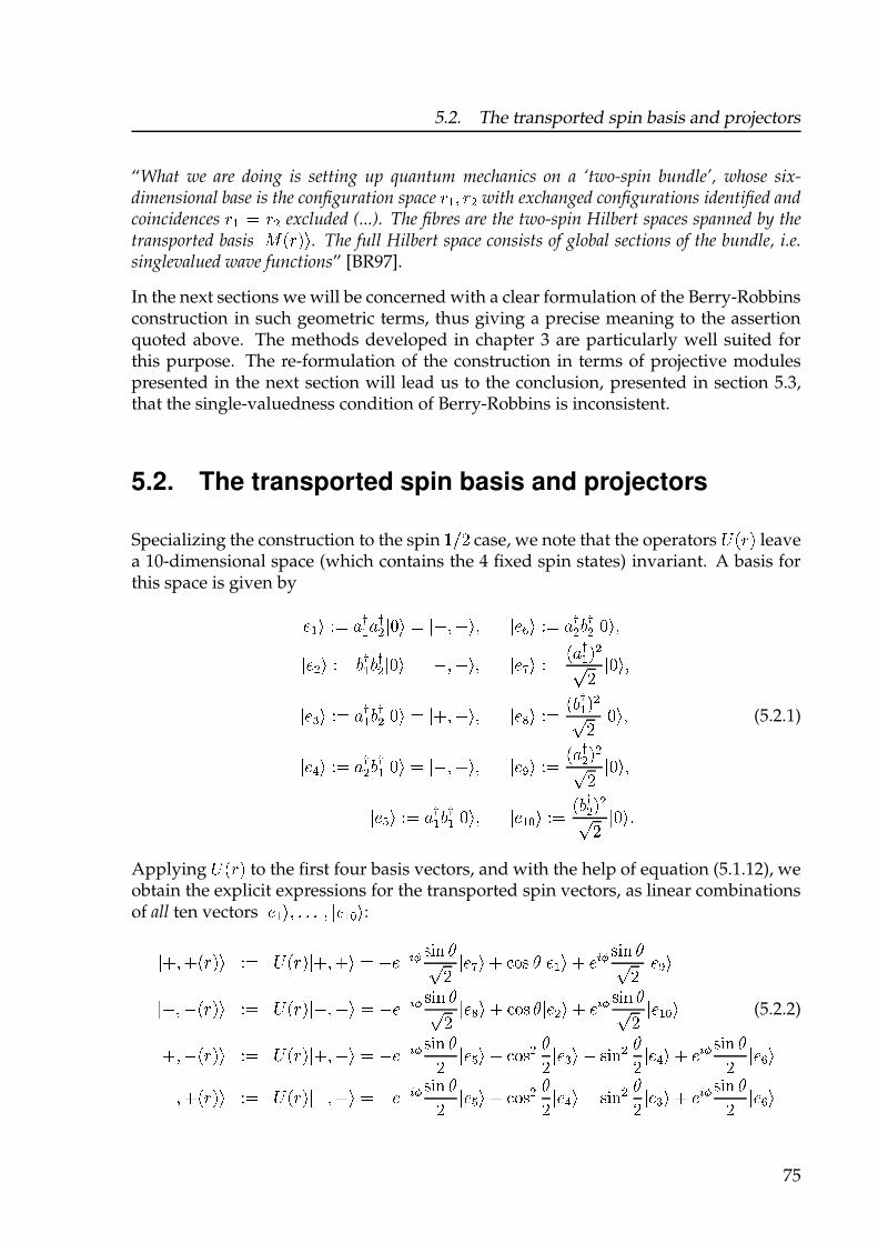
5.2. The transported spin basis and projectors
“What we are doing is setting up quantum mechanics on a ‘two-spin bundle’, whose six-dimensional base is the configuration space � � � �� with exchanged configurations identified andcoincidences � � � �� excluded (...). The fibres are the two-spin Hilbert spaces spanned by thetransported basis �� �� ��. The full Hilbert space consists of global sections of the bundle, i.e.singlevalued wave functions” [BR97].
In the next sections we will be concerned with a clear formulation of the Berry-Robbinsconstruction in such geometric terms, thus giving a precise meaning to the assertionquoted above. The methods developed in chapter 3 are particularly well suited forthis purpose. The re-formulation of the construction in terms of projective modulespresented in the next section will lead us to the conclusion, presented in section 5.3,that the single-valuedness condition of Berry-Robbins is inconsistent.
5.2. The transported spin basis and projectors
Specializing the construction to the spin ��� case, we note that the operators � �� � leavea 10-dimensional space (which contains the 4 fixed spin states) invariant. A basis forthis space is given by
�� �� �� !� !� �"� � �# � # � � ��$ � �� !� %!� �"� ���� � �� %!�%!� �"� � �& � &� � ��' � �� � !� ��(� �"� ���) � �� !�%!� �"� � �# � &� � ��* � �� �%!� ��(� �"� � (5.2.1)
��+ � �� !� %!� �"� � �& � # � � ��, � �� � !� ��(� �"� ���- � �� !�%!� �"� � �� �. � �� �%!� ��(� �"� /
Applying � �� � to the first four basis vectors, and with the help of equation (5.1.12), weobtain the explicit expressions for the transported spin vectors, as linear combinationsof all ten vectors �� �� � / / / � �� �. �:
�# � # �� �� �� � �� � �# � # � � &�012 345 6(� ��' � # 783 6 �� �� # �12 345 6(� ��, ��& � & �� �� �� � �� � �& � &� � &�012 345 6(� ��* � # 783 6 ��� � # �12 345 6(� �� �. � (5.2.2)
�# � & �� �� �� � �� � �# � &� � &�012 345 6� ��- � # 783� 6� ��) � & 345� 6� ��+ � # �12 345 6� ��$ ��& � # �� �� �� � �� � �& � # � � &�012 345 6� ��- � # 783� 6� ��+ � & 345� 6� ��) � # �12 345 6� ��$ �
75

5. Applications to the Berry-Robbins approach to Spin-Statistics
The transported spin vectors are maps9 : ;< => ?;< @A B> CD(= E
spanF @G HD I J J J I @G HK DL). Because of the relation@A B;> CD E ; @A B> CD, it is not pos-
sible to regard them as maps M N : < =(because of equation (5.1.14), this is indeed
possible for the whole wave function@O B> CD). But this situation changes if we make a
change to a basis of total angular momentum. First, we define the following auxiliaryvectors: @P I ; PDQRST UE @GV D @PI ;PDQWT UE @G: D @PI ; PDQST UE @G HK D@PI XDQRST UE @GY D @PI XD QWT UE HZ: B@G[ D \ @G] DC @PI XD QST UE @G^ D@PI PDQRST UE @G_ D @PI PD QWT UE @G HD @PI PD QST UE @G` D@X I XD UE HZ: B @G[ D ; @G] DC JApplying a B> C to them, we obtain:
a B> C @PI b DQRST E cde: fg @PI b DQRST \ Ghi ejk flg @PI b DQWT \ G:hi ejk : fg @PI b DQSTa B> C @PI b DQWT E ;Gmhi ejk flg @PI b DQRST \ cde f @PI b DQWT \ Ghi ejk flg @PI b DQST (5.2.3)
a B> C @PI b DQST E Gm:hi ejk : fg @PI b DQRST ; Gmhi ejk flg @PI b DQWT \ cde: fg @PI b DQSTa B> C @X I XD E @X I XD J
For the physical spin vectors (with@PI X B> CD UE BPnlgCB @\ I ; B> CD \ @; I \ B> CDC, etc..) one
then gets
@P I P B> CD E ;Gmhi ejk flg @PI PD QRST \ cde f @PI PD QWT \ Ghi ejk flg @PI PD QST@P I X B> CD E ;Gmhi ejk flg @PI XD QRST \ cde f @PI XD QWT \ Ghi ejk flg @PI XD QST (5.2.4)
@P I ; PB> CD E ;Gmhi ejk flg @PI ;PDQRST \ cde f @PI ;PDQWT \ Ghi ejk flg @PI ; PDQST@X I X B> CD E @X I XD JNote that the vectors
@o I b B> CD (forBo I b C E BPI p PCI BPI X C and
BX I X C) are all non van-ishing for all > . Thus, we see that > ?< @o I b B> CD is a section in a bundle with totalspace
9 : q =r, where
=ris the space spanned by F @PI b DQRST I @P I b DQWT I @P I b DQST L, wheno E P
and the space spanned by@X I XD, when
o E X. All four line bundles are trivial,since the corresponding sections are non vanishing. The difference lies in the symme-try/antisymmetry of the sections with respect to > , when they are regarded as vectorvalued functions on the sphere. This symmetry/antisymmetry could be regarded as
76

5.2. The transported spin basis and projectors
an equivariance property with respect to some st action on each line bundle, but thisis something we do not have at our disposal, so we will consider these line bundlesas bundles over the sphere. One can then construct the corresponding projectors. Theinteresting thing about constructing these projectors is that the three corresponding tou v w
turn out to have matrix components which are even functions. One can then in-terpret these projectors as defining projective modules over x yz { t |
and, as we will see,the form of these projectors is exactly the same as the one displayed in equation(4.2.20).Since the first three basis vectors in equation (5.2.4) have the same form, let us considerany of them, written in the form
}~ y� |� v ����� ��� ��� }� �� � ��� � }�t � � ��� ��� ��� }�� � �(5.2.5)
The (�-dependent) operator{ y� | that projects onto the vector space spanned by
}~ y� |�is defined by
{ y� | }�� � �v �~ y� | }�� � }~ y� |�. Explicitly, we have:
{ y� | }� �� v ���t �� }� �� � ��� � ��� ��� ��� }�t � � ���t �� �t�� }�� �{ y� | }�t � v � ��� � ��� ��� ���� }� �� � ���t � }�t � � ��� � ��� ��� ��� }�� �
(5.2.6)
{ y� | }�� � v � ��� t �� ��t�� }� �� � ��� � ��� ��� ���� }�t � � ���t �� }�� �In the basis � }�� ���, { y� | has a matrix form, with components ��� y� | defined by{ y� | }�� � v �� �� � y� | }�� �, so that
� y� | v ����t ��� t � � ��t ��� � ��� ����� � �t ��� t ���t��� ��t ��� � ��� ���� ���t � ��t ��� � ��� ������ �t ��� t ��t�� ��t ��� � ��� ���� �t ���t �
�� �(5.2.7)
We have thus obtained, from the transported spin basis, exactly the same expressionfor the projector that was considered in proposition 4.2.2. Here we are considering it asdefining a projective module over the algebra x y¡ t |
, but given that its components areeven functions, we could in principle consider it as giving place to a projective moduleover x yz { t |
. This point of view will be considered in more detail in the next section.
Let us now use the obtained expression for the projector to show that each spin basisvector is a section of a line bundle (determined by the projector
{ y� |) that is parallelwith respect to the connection
{ ¢. Writing
}~ y� |� v � � ~� y� | }�� � and £~ v y~ � ¤ ~t ¤ ~� | v77

5. Applications to the Berry-Robbins approach to Spin-Statistics
¥¦§¨©ª «¬ ®¯°±² ³´« ® ² §©ª «¬ ® ¯°±µ, we have:¶ · ¸¹ ¥º µ» ¼ ¶ ½© ·¹© ¥º µ ¸§© »¼ ½© ·¹© ¥º µ¶ ¸§¾ »¼ ½©¿¾ ·¹© ¥º µÀ¾ © ¥º µ ¸§¾ »¼ ½¾ ¥À ¥º µ Á · ¹ ¥º µµ¾Ã ÄÅ ÆÇÈ ¸§¾ »¼ É Ê
(5.2.8)
This also shows that the parallel transport condition (third condition in definition 5.1.1)holds if and only if
¸¹ » is parallel transported with respect to the connection Ë ¼ ¶ ·,
because¸¹ » is nowhere vanishing, so that
À ¥º µ Á · ¹ ¥º µ ¼ Éexactly when ̹ ¥º µ ¸·¹ ¥º µ» ¼É
.
In this section we have shown how, for the spin ͯ± case, the transported spin basisgives place to a projector which contains, as direct summands, one copy of the triv-ial rank one projector and three copies of the projector from proposition 4.2.2, i.e., aprojective module isomorphic to Ψ. Although it will not be done here, let us remarkthat, in the case of general spin, the transported spin basis constructed with the helpof Schwinger’s oscillators also gives place to a projective module. In the same way asin the case Ï ¼ ͯ±, after passing to the total angular momentum basis and decom-posing the spin states according to the Clebsch-Gordan decomposition, one obtains aprojective module that contains different copies of ÎÐ and Ψ. Hence, concerning thegeometric properties of the transported spin basis, it is enough to consider the caseÏ ¼ ͯ±.
5.3. Single-valuedness of the wave function
As we have already pointed out, the requirement of single-valuedness imposed on thewave function in the form of equation (5.1.14) is an essential ingredient of the Berry-Robbins construction. In this subsection we will discuss that requirement, using thetools developed so far. We shall arrive at the conclusion that the single-valuednesscondition of Berry and Robbins leads to a contradiction.
There are two instances -not altogether independent- where the concept of a “multiple-valued function” comes into play in the present context. Notice that this concept isactually related to the transformation properties of the function under a certain sym-metry group. Before describing them, let us remark that physicists do not necessarilyuse the term “multiple-valued” in the same way mathematicians do. So, for example,
78
5.3. Single-valuedness of the wave function
in the theory of one complex variable, the function Ñ ÒÓ ÔÑ is said to be multiple-valued, because there are two possible solutions (for Õ ) to the equation Õ Ö × Ñ . Incontrast to this, consider the wave function of a spin ØÙÚ particle. As a “mathematical”function, it is a single-valued one. But it has the property that, under a ÚÛ rotation,it is not left unchanged: its value after the rotation is ÜÝØÞ times its original value;hence the usage of the term “double-valued” in the physics literature. The physicalneed to impose single-valuedness was examined already in the early days of Quan-tum Mechanics. In particular, Pauli studied the problem and showed that consideringmultiple-valued functions (in the “mathematical”sense described above) leads to prob-lems with the self-adjointness of related operators (see [Pau33, Pau39]). For a furtheranalysis of the status of single-valuedness in physics (and in particular in view of ef-fects like the Aharanov-Bohm), the reader is referred to [Mer62] and references therein.
Thus, we will also adopt the point of view that, as a “mathematical function” definedon configuration space, the wave function should be single-valued. Now, in the par-
ticular case of ß identical particles, depending on which of the spaces ( àá × â ãä å æ orá × Üâ ãä åæ ÞÙçä ) is considered as the physical one, one will impose single-valuednessto the wave function, whose domain of definition will be the physical configurationspace. As argued in [LM77], due to Gibbs’ paradox, in our case the physical configu-
ration space should be chosen asá
, and not as àá. In the configuration space approachto Spin-Statistics, this is perhaps one of the few points on which most authors agree.
Once we have chosená
as configuration space, we are faced with the fact that, dueto the non-trivial global structure of
á, different possibilities for the definition of the
wave function arise: It will be, in general, a cross-section of some vector bundle overá. As already pointed outè, a section of a vector bundle is sometimes regarded as a
multiple-valued function, because of the different functions that are needed in order todescribe it in terms of local trivialisations. But let us, once again, remark that a sectionof a vector bundle is a single-valued map, even if the bundle is not trivial. This is thefirst instance we alluded to above.
The advantages of working on àá -the universal cover ofá
- are well known and havebeen used extensively (see e.g. [HMS89, Mor92]). In particular, every wave function é ,
being a section of some bundle overá
, can be brought to the form of a map àé ê àá Ó ë ì .Although this map is a single-valued one, it is of common usage, in the physics liter-ature, to call it a “multiple-valued function”. From the discussion at the beginning
of section 3.3, we know that àé should rather be referred to as an equivariant func-
tion. Once we know the value of àé at some point íî ï àá, we can use the equivarianceproperty to find its value at all points ð ñ íî , for ð ï çä . But the different points ð ñ íîdo represent one and the same physical configuration; hence the tendency to call àé a“multiple-valued function”. This is the second instance we alluded to above.
It is our impression that, instead of talking about single-valuedness, one should con-sider the notion of well-definiteness. In fact, the point with many of the standard exam-ò
See the remark on the fourth paragraph of section 1.2
79

5. Applications to the Berry-Robbins approach to Spin-Statistics
ples where single-valuedness comes into play, having so far-reaching consequences as,for example, the quantization of angular momentum, is not really single-valuednessbut well-definiteness. Considering the example of angular momentum, what is being
“forced” when a condition of the form ó ôõ ö ÷ø ó ôõ ù úû ö is imposed, is that ó , as a mapó ü ý þ ÿ � , be well defined. The imposition of this condition is necessary because ý þ isbeing described using only one local chart. In a global formulation, this problem wouldnot even arise. Saying that ó belongs to � ôý þö automatically implies well-definitenessand, for that matter, also single-valuedness. The origin of the quantization of angularmomentum is thus not so much due to the fact that ó be single-valued, but to the factthat ý þ is a compact manifold, from which it follows that the spectrum of �� is discrete.
Before embarking on a discussion of the single-valuedness condition of Berry-Robbins,let us summarize the situation as follows:
We are given a configuration space � with û þ ô�ö �ø �. Physical wave functions willbe, in general, of the form ó � � ô� ö, for some vector bundle over �. Because oftheorem 3.3.5 we know that, as a module over � ô�ö, �� ô� ö is isomorphic to � ô ö,where � ü �� ÿ � and � ø û þ ô�ö. Thus, ó � � ô� ö is isomorphically represented by�ó � �� ô �� � ö. If, as in the case of our interest, the bundle is flat, � will be a trivial
bundle and we might as well consider �ó to be a usual function, taking values in some� � .
With these preliminary remarks in mind, we proceed now to interpret the Berry-Robbins single-valuedness condition, within our formalism. Consider a wave func-tion for two spin � particles written in terms of a transported spin basis � �� ô� ö��,
�� ô� ö� ø �� �� ô� ö �� ô� ö� � (5.3.1)
The transported spin vectors will be assumed to satisfy the exchange rule � �� ô�� ö� øô��ö �� ô� ö�. The choice of ! will be left open for the moment. Notice, however,that it is possible to construct a spin basis satisfying the three requirements originallyimposed by Berry-Robbins on the spin basis, irrespectively of the value of ! . Changingto the total angular momentum (� �" # ��) basis, we can re-write the exchange conditionas follows:
�" # ô�� ö� ø ô��ö$% &' ( �" # ô� ö� � (5.3.2)
The vectors �� ô� ö� are all non-vanishing, by assumption. It follows that all the vectors�" # ô� ö� are non-vanishing, so that they give place to a trivial vector bundle ) BR overthe sphere, with total space* ô) BR ö ø � ô� �' +, -' +, �" # ô� ö� ö � � � ý $ -' +, � � �� (5.3.3)
Let us remark that, for any choice of the spin basis (including the choice of ! ), thebundles ) BR are all isomorphic to the trivial bundle ý $ . � $ /$0( þ1 ÿ � $ /$0( þ1 . But, given
80

5.3. Single-valuedness of the wave function
we are interested, in particular, in the transformation properties of the spin basis underexchange, we keep track of the sign 23456 by means of a sub-index in 7 BR6 . Hence, 7 BR6denotes the explicit realization of the bundle with total space given by eq. (5.3.3),and not the equivalence class of this bundle. Similarly, from now on we will alsolabel the spin basis elements and functions constructed from them with a sub-index8
: 9: 2; 5<6 = 9> = ? 2; 5<6 and 9@ 2; 5<6 .
9@ <6 is a map ; AB 9@ 2; 5<6 from C D to some vector space, but it gives place to a section@6 E F 2C D = 7 BR6 5, defined by@6 2; 5 GH 2; = 9@ 2; 5<6 5. In any case, 9@ 2; 5<6 is supposed
to represent the physical wave function, and this one should have I J D as domain ofdefinition. This is the reason for the imposition of the single-valuedness condition.
In order to make the arguments presented below as clear as possible, let us highlightthe following three features of the Berry-Robbins approach:
(A) Exchange rule: 9 K: 23; 5<6 H 23456 9: 2; 5<6 .
(B) Single-valuedness: 9@ 23; 5<6 LH 9@ 2; 5<6 .
(C) Berry and Robbins statement, quoted at the endof section 5.1, that 9@ 2; 5<6 represents a section ofa bundle over I J D .
According to our previous discussion, the physical wave function M is a section ofsome vector bundle N over I J D : M E F 2I J D = N 5. In order to make contact with theBerry-Robbins approach, we will make use of the results of chapter 3. Recall that theprojection O G C D B I J D induces a natural PD-action QR on the pull-back bundle O SN andthat, according to theorem 3.3.5, the space of invariant sections (with respect to QR ) ofO SN is isomorphic, as a T 2I J D 5-module, to the space of sections of N :
UVW G F 2I J D = N 5 XY3B FZ[ 2C D = O SN 5\This means, in particular, that we can represent the wave function M as a section
UVW 2M 5of the bundle O SN . But O SN is a trivial bundle and has the same rank as 7 BR6 , so that wealso have isomorphisms O SN ]H 7 BR6 , for any choice of
8. Now recall that, in order to
regard a section in 7 BR6 as a section in N , we must require it to be PD-invariant. Theaction in 7 BR6 (which is not present within the Berry-Robbins approach) must thereforebe defined in such a way that the isomorphism O SN ]H 7 BR6 still holds as an isomorphismof PD bundles. In this way, we can realize M as a map of the form (5.3.1), if we requirethe section ; AB 2; = 9@ 2; 5<6 5 to be invariant with respect to the PD-action of 7 BR6 .
81
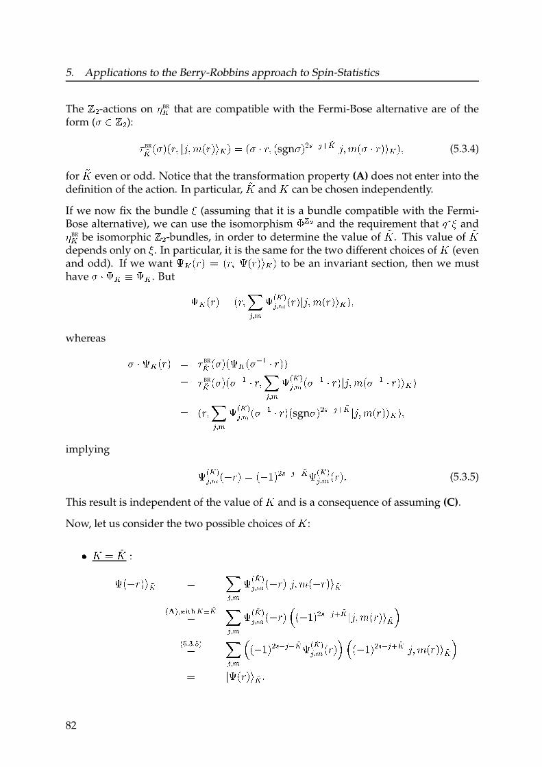
5. Applications to the Berry-Robbins approach to Spin-Statistics
The ^_-actions on ` BRa that are compatible with the Fermi-Bose alternative are of theform (b c ^_):
d BRea fb gfh i jk i l fh gma g n fb o h i fsgnb g_pqr s ea jk i l fb o h gma gi (5.3.4)
for tu even or odd. Notice that the transformation property (A) does not enter into thedefinition of the action. In particular, tu and
ucan be chosen independently.
If we now fix the bundle v (assuming that it is a bundle compatible with the Fermi-Bose alternative), we can use the isomorphism wxy and the requirement that z {v and` BRa be isomorphic ^_-bundles, in order to determine the value of tu . This value of tudepends only on v . In particular, it is the same for the two different choices of
u(even
and odd). If we want |a fh g n fhi j| fh gma g to be an invariant section, then we musthave b o |a } |a . But
|a fh g n fhi~r �� | �a �r �� fh g jk i l fh gma giwhereas
b o |a fh g n d BRea fb gf|a fb q� o h ggn d BRea fb gfb q� o h i~r �� | �a �r �� fb q� o h g jk i l fb q� o h gma gn fh i~r �� | �a �r �� fb q� o h g fsgnb g_pqr s ea jk i l fh gma gi
implying
| �a �r �� f�h g n f��g_pqr s ea | �a �r �� fh g� (5.3.5)
This result is independent of the value ofu
and is a consequence of assuming (C).
Now, let us consider the two possible choices ofu
:
� u n tu �j| f�h gm ea n ~r �� | � ea �r �� f�h g jk i l f�h gm ea
�� � �� ��� a � ean ~r �� | � ea �r �� f�h g �f��g_pqr s ea jk i l fh gm ea ��� �� �� �n ~r �� �f��g_pqr s ea | � ea �r �� fh g� �f��g_pqr s ea jk i l fh gm ea �n j| fh gm ea �
82
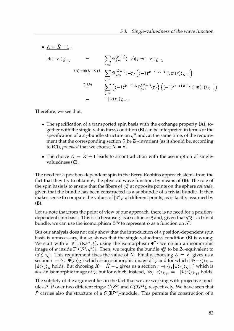
5.3. Single-valuedness of the wave function
� � � �� � � ��� ��� ¡ ¢£¤ ¥ � ¦§ ¨© � ª ¢£ ¤ ¥«§ ¨© ��� �¬ ® ��� ¡ ¢£ ¤ ¥
ª¯ « ¨° ±²³ £ ´ ¢£¤ ¥� ¦§ ¨© � ª ¢£ ¤ ¥«§ ¨© ��� µ��� ¶·¸§ ¤ ¢£ ¤ ¥ �¬ ® �� ¡ ¢£ ¤ ¥¹ªº »¼ »º «� ¦§ ¨© µ��� ¶·¸§ ¤ ¢£ � ª ¢£ ¤ ¥«§ ¨© �� ¹ µ��� ¶·¸§ ¤ ¢£ ¤ ¥ �¬ ® �� ¡ ¢£ ¤ ¥¹� � �� �� ¡ ¢£¤ ¥ ½
Therefore, we see that:
� The specification of a transported spin basis with the exchange property (A), to-gether with the single-valuedness condition (B) can be interpreted in terms of thespecification of a ¾¶-bundle structure on ¿ BR£ and, at the same time, of the require-ment that the corresponding section
�be ¾¶-invariant (as it should be, according
to (C)), provided that we choose � � �� .� The choice � � �� � � leads to a contradiction with the assumption of single-valuedness (C).
The need for a position-dependent spin in the Berry-Robbins approach stems from thefact that they try to obtain À , the physical wave function, by means of (B): The role ofthe spin basis is to ensure that the fibers of ¿ BR£ at opposite points on the sphere coincide,given that the bundle has been constructed as a subbundle of a trivial bundle. It thenmakes sense to compare the values of
�� ¡£ at different points, as is tacitly assumed by(B).
Let us note that,from the point of view of our approach, there is no need for a position-dependent spin basis. This is so because À is a section of Á and, given that  ÃÁ is a trivialbundle, we can use the isomorphism ÄÅÆ to represent À as a function on Ç ¶.But our analysis does not only show that the introduction of a position-dependent spinbasis is unnecessary, it also shows that the single-valuedness condition (B) is wrong:We start with À È É �Ê Ë ¶ Á , using the isomorphism ÄÅÆ we obtain an isomorphicimage of À inside ÉÌÍ �Ç ¶  ÃÁ . Then, we require the bundle ¿ BR£ to be ¾¶-equivalent to� ÃÁ ÎÏ . This requirement fixes the value of �� . Finally, choosing � � �� gives us asection
� ÐÑ �� �� �� ¡ ¢£ which is an isomorphic image of À and for which�� ��� ¡ ¢£ ��� �� ¡ ¢£ holds. But choosing � � �� � � gives us a section
� ÐÑ �� �� �� ¡ ¢£¤ ¥ which isalso an isomorphic image of À , but for which, instead,
�� ��� ¡ ¢£ ¤ ¥ � � �� �� ¡ ¢£ ¤ ¥ holds.
The subtlety of the argument lies in the fact that we are working with projective mod-
ules ÒË Ëover two different rings: Ó �Ç ¶ and Ó �Ê Ë ¶
, respectively. We have seen thatÒË carries also the structure of a Ó �Ê Ë ¶ -module. This permits the construction of a
83

5. Applications to the Berry-Robbins approach to Spin-Statistics
Ô ÕÖ × Ø Ù-module homomorphism ÚÛÜ Ý × Þ ß×
(thm. 3.3.5) that maps×
isomorphically
onto a submodule ofß×
(here considered asÔ ÕÖ × Ø Ù
-module). The important point is,
then, to recognize the correct condition characterizing those elements ofß×
that lie inÚÛÜ Õ× Ù. As we have seen, this condition is expressed in the form
à á â ã â Õà ä åØ Ùæ (5.3.6)
a form that (to our opinion), while retaining the original motivation behind the single-valuedness condition, is free from ambiguities and mathematically correct. Physically,because of indistinguishability, the wave function is defined on
Ö × Ø. Working on ç Ø
thus demands the introduction of some criterion that allows one to retain the correctphysical interpretation. Although this might be the purpose of the single-valuednesscondition of Berry-Robbins, we have seen in detail why the condition itself is not ten-able. Instead we propose the imposition of invariance on the wave function (when de-fined on ç Ø) as stated in equation (5.3.6) as a more clear and concise way to incorporateindistinguishability into the (usual) formalism of Quantum Mechanics.
Let us remark that, in [HR04] a generalization of the BR construction to è particles hasbeen given. Being based on the same assumptions (in particular the single-valuednesscondition), it has the same problems as the one for two particles. The extension ofour reasoning to that -more general- case is nevertheless straightforward, since ourapproach is model-independent.
84
6. Further developments
In this work, almost all of our attention has been directed towards a reformulation ofthe Berry-Robbins (BR) proposal in geometric/algebraic terms. This effort, per se, doesnot seem to provide an advance regarding the Spin-Statistics theorem. But it must besaid that the BR proposal has generated, in last few years a growing interest in theissue of Spin-Statistics in (non-relativistic) Quantum Mechanics. It is for this reasonthat we have emphasized so much the problems of their approach. We have seen thatthe problems with the BR proposal are of a conceptual nature. This means that now wehave to turn our attention to other directions. Two points that, to our opinion, deserveto be investigated further are the correct incorporation of spin degrees of freedom intothe configuration space approach and a convincent proof of the Fermi-Bose alternative,of a geometric nature. As we will see below, it seems that these two questions areclosely related.
It is natural, for reasons of simplicity, to attack these and other questions first at thelevel of a two particle system, the hope being always that, once the two particle case hasbeen understood, the general, many-particle case can be understood without essentialmodifications. But if one is also interested in the relation of the geometric/topologicalcharacter of quantum indistinguishability to the (relativistic QFT) Spin-Statistics con-nection, then a formalism able to handle any number of particles will be welcome. Inthis work we have performed all explicit computations in the two particle case, but themotivation for the approach presented in chapter 3 has been, precisely, to develop aformalism that (1) allows to understand and clarify alternative approaches and (2) can,potentially, be applied to the case of an arbitrary number of particles. Also, inspiredby the philosophy of Non-commutative Geometry, one could think of improving theapproach in such a way that, while retaining all the geometric properties inherent toquantum indistinguishability, is also formulated in a language, of more algebraic na-ture, that could help to build a bridge to QFT. Although certain attempts more or lessrelated to this idea have been made (see, e.g. [Tsc89]), there are, at the moment, noconcrete results.
In this last chapter we will, therefore, consider in some detail some of the points onwhich we think it is possible to make some advance in the near future.
85

6. Further developments
6.1. éê ëìí and Spin
When quantum mechanics is studied in a more general setting, such as the one wehave been discussing in the previous chapters where the wave function is consideredto be a section in a vector bundle, a reconsideration of many physical concepts becomesnecessary. A particularly important one is angular momentum and, closely related toit, the definition of spin.
Let us start by considering the simplest possible example: A spin îïð particle in 3dimensions. In this case, one considers the state spaceñ ò óô õö ÷ ø ù ú ûüýôþ ÿThe spin state space
ú ûüýôþhas a basis � �� � � ����
with respect to which the wave func-tion can be written: � ò �� ù �� � � � ù ��� ÿThe spin operators � � ÷ are, by definition, operators representing � õðø, acting onú ûüýôþ
by � �� � ò �� �� �� � ò �÷ �� � ò � îð �� � ÿTogether with the angular momentum operators
ó �, they give place to infinitesimal
generators of rotations, acting onñ
:�� ò ó � ùId� ����� �
Id�� û�� þ ù � ÿ(6.1.1)
The infinitesimal generatorsó �
and �give, by exponentiation, the respective repre-
sentations of the whole group � õðø onóô õö ÷ ø
andú ûüýôþ
. Explicitly, one has, for� � � õðø: õ� �� ø õ! ø ò �� õ� ü! ø� �� � ò " üýô õ� ø �� � ÿConsequently, the total wave function transforms under � õðø as
� # � $ ò � �, with� �
defined by: õ� � ø õ! ø %ò " ûüýôþ õ� ø õ� õ� ü! øø ÿ (6.1.2)
Looking back at equation (3.3.5), we see that by regarding the wave function as a sec-tion of the trivial bundle & ÷ ' ú üýô # & ÷ , the transformation of the wave functionunder rotations is the one induced from the following � õðø-action on the bundle:( % � õðø ' õ& ÷ ' ú üýô ø �# õ& ÷ ' ú üýô ø
(6.1.3)õ� � õ! � ) øø *�# õ� ! � " ûüýôþ õ� ø) ø86
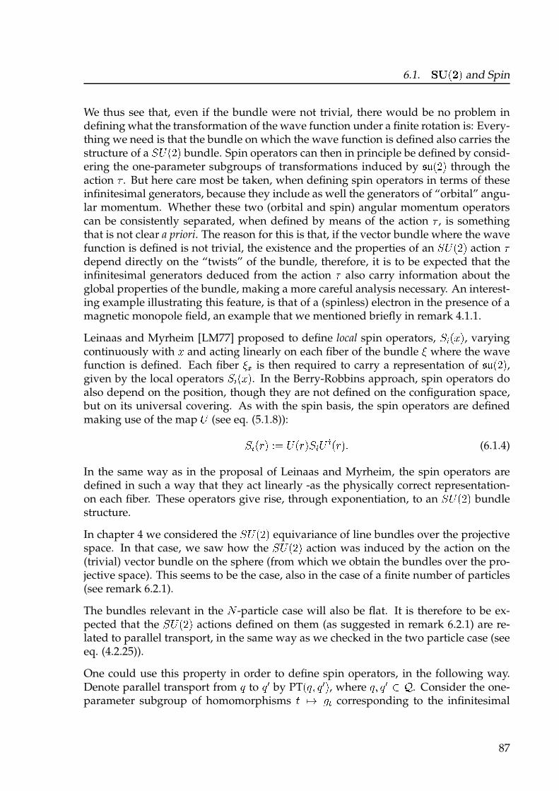
6.1. +, -./ and Spin
We thus see that, even if the bundle were not trivial, there would be no problem indefining what the transformation of the wave function under a finite rotation is: Every-thing we need is that the bundle on which the wave function is defined also carries thestructure of a 0 1 -2/ bundle. Spin operators can then in principle be defined by consid-ering the one-parameter subgroups of transformations induced by 34 -2/ through theaction 5 . But here care most be taken, when defining spin operators in terms of theseinfinitesimal generators, because they include as well the generators of “orbital” angu-lar momentum. Whether these two (orbital and spin) angular momentum operatorscan be consistently separated, when defined by means of the action 5 , is somethingthat is not clear a priori. The reason for this is that, if the vector bundle where the wavefunction is defined is not trivial, the existence and the properties of an 0 1 -2/ action 5depend directly on the “twists” of the bundle, therefore, it is to be expected that theinfinitesimal generators deduced from the action 5 also carry information about theglobal properties of the bundle, making a more careful analysis necessary. An interest-ing example illustrating this feature, is that of a (spinless) electron in the presence of amagnetic monopole field, an example that we mentioned briefly in remark 4.1.1.
Leinaas and Myrheim [LM77] proposed to define local spin operators, 06 -7 /, varyingcontinuously with 7 and acting linearly on each fiber of the bundle 8 where the wavefunction is defined. Each fiber 89 is then required to carry a representation of 34 -2/,given by the local operators 06 -7 /. In the Berry-Robbins approach, spin operators doalso depend on the position, though they are not defined on the configuration space,but on its universal covering. As with the spin basis, the spin operators are definedmaking use of the map 1 (see eq. (5.1.8)):06 -: / ;< 1 -: /06 1 = -: /> (6.1.4)
In the same way as in the proposal of Leinaas and Myrheim, the spin operators aredefined in such a way that they act linearly -as the physically correct representation-on each fiber. These operators give rise, through exponentiation, to an 0 1 -2/ bundlestructure.
In chapter 4 we considered the 0 1 -2/ equivariance of line bundles over the projectivespace. In that case, we saw how the 0 1 -2/ action was induced by the action on the(trivial) vector bundle on the sphere (from which we obtain the bundles over the pro-jective space). This seems to be the case, also in the case of a finite number of particles(see remark 6.2.1).
The bundles relevant in the ? -particle case will also be flat. It is therefore to be ex-pected that the 0 1 -2/ actions defined on them (as suggested in remark 6.2.1) are re-lated to parallel transport, in the same way as we checked in the two particle case (seeeq. (4.2.25)).
One could use this property in order to define spin operators, in the following way.Denote parallel transport from @ to @ A by PT-@ B @ A /, where @ B @ A C D. Consider the one-parameter subgroup of homomorphisms E FG HI corresponding to the infinitesimal
87
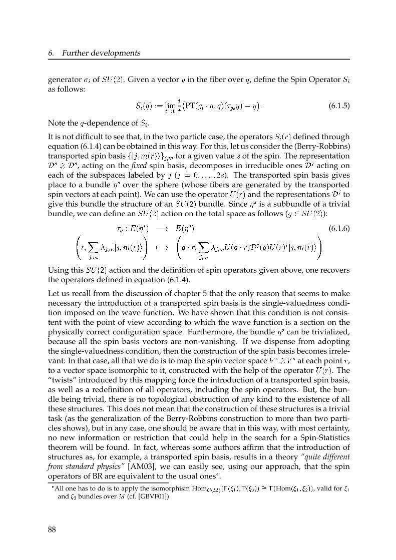
6. Further developments
generator JK of L M NOP. Given a vector Q in the fiber over R , define the Spin Operator LKas follows: LK NR P ST UVWXYZ [\ ]PTN^X _ R ` R P Nabc Q P d Q ef (6.1.5)
Note the R-dependence of LK.It is not difficult to see that, in the two particle case, the operators LK Ng P defined throughequation (6.1.4) can be obtained in this way. For this, let us consider the (Berry-Robbins)transported spin basis h ij ` k Ng Plmn op for a given value q of the spin. The representationr s t r s
, acting on the fixed spin basis, decomposes in irreducible onesr n
acting oneach of the subspaces labeled by
j(j T u ` f f f ` Oq). The transported spin basis gives
place to a bundle v sover the sphere (whose fibers are generated by the transported
spin vectors at each point). We can use the operator M Ng P and the representationsr n
togive this bundle the structure of an L M NOP bundle. Since v s
is a subbundle of a trivialbundle, we can define an L M NOP action on the total space as follows (^ w L M NOP):ab S x Nv s P dy x Nv s P (6.1.6)zg` {n op |n op ij ` k Ng Pl} ~dy z^ _ g ` {n op |n op M N^ _ g Pr n N^ PM Ng P� ij ` k Ng Pl}Using this L M NOP action and the definition of spin operators given above, one recoversthe operators defined in equation (6.1.4).
Let us recall from the discussion of chapter 5 that the only reason that seems to makenecessary the introduction of a transported spin basis is the single-valuedness condi-tion imposed on the wave function. We have shown that this condition is not consis-tent with the point of view according to which the wave function is a section on thephysically correct configuration space. Furthermore, the bundle v s
can be trivialized,because all the spin basis vectors are non-vanishing. If we dispense from adoptingthe single-valuedness condition, then the construction of the spin basis becomes irrele-vant: In that case, all that we do is to map the spin vector space � s t � s
at each point g ,to a vector space isomorphic to it, constructed with the help of the operator M Ng P. The“twists” introduced by this mapping force the introduction of a transported spin basis,as well as a redefinition of all operators, including the spin operators. But, the bun-dle being trivial, there is no topological obstruction of any kind to the existence of allthese structures. This does not mean that the construction of these structures is a trivialtask (as the generalization of the Berry-Robbins construction to more than two parti-cles shows), but in any case, one should be aware that in this way, with most certainty,no new information or restriction that could help in the search for a Spin-Statisticstheorem will be found. In fact, whereas some authors affirm that the introduction ofstructures as, for example, a transported spin basis, results in a theory “quite differentfrom standard physics” [AM03], we can easily see, using our approach, that the spinoperators of BR are equivalent to the usual ones�.�
All one has to do is to apply the isomorphism Hom� �� � �� ��� � � � ��� �� �� � �Hom�� � � �� ��, valid for ��and �� bundles over � (cf. [GBVF01])
88
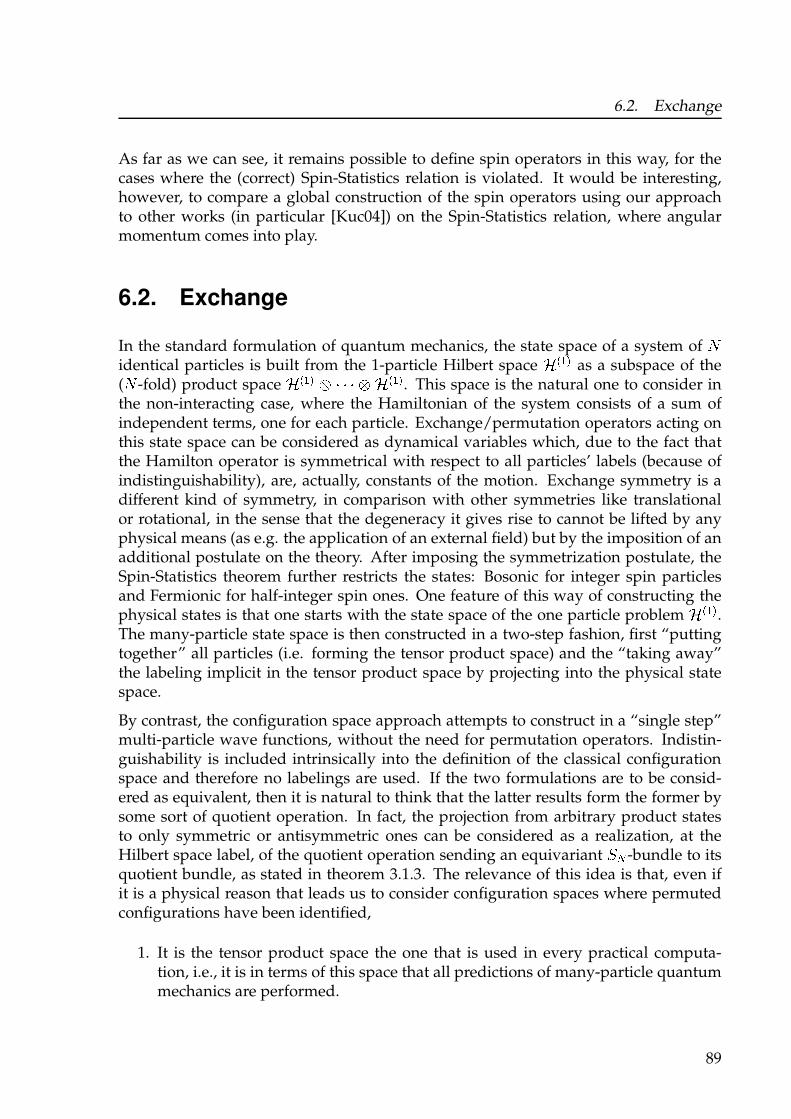
6.2. Exchange
As far as we can see, it remains possible to define spin operators in this way, for thecases where the (correct) Spin-Statistics relation is violated. It would be interesting,however, to compare a global construction of the spin operators using our approachto other works (in particular [Kuc04]) on the Spin-Statistics relation, where angularmomentum comes into play.
6.2. Exchange
In the standard formulation of quantum mechanics, the state space of a system of �identical particles is built from the 1-particle Hilbert space � ��� as a subspace of the(� -fold) product space � ��� � � � � � � ���. This space is the natural one to consider inthe non-interacting case, where the Hamiltonian of the system consists of a sum ofindependent terms, one for each particle. Exchange/permutation operators acting onthis state space can be considered as dynamical variables which, due to the fact thatthe Hamilton operator is symmetrical with respect to all particles’ labels (because ofindistinguishability), are, actually, constants of the motion. Exchange symmetry is adifferent kind of symmetry, in comparison with other symmetries like translationalor rotational, in the sense that the degeneracy it gives rise to cannot be lifted by anyphysical means (as e.g. the application of an external field) but by the imposition of anadditional postulate on the theory. After imposing the symmetrization postulate, theSpin-Statistics theorem further restricts the states: Bosonic for integer spin particlesand Fermionic for half-integer spin ones. One feature of this way of constructing thephysical states is that one starts with the state space of the one particle problem � ���.The many-particle state space is then constructed in a two-step fashion, first “puttingtogether” all particles (i.e. forming the tensor product space) and the “taking away”the labeling implicit in the tensor product space by projecting into the physical statespace.
By contrast, the configuration space approach attempts to construct in a “single step”multi-particle wave functions, without the need for permutation operators. Indistin-guishability is included intrinsically into the definition of the classical configurationspace and therefore no labelings are used. If the two formulations are to be consid-ered as equivalent, then it is natural to think that the latter results form the former bysome sort of quotient operation. In fact, the projection from arbitrary product statesto only symmetric or antisymmetric ones can be considered as a realization, at theHilbert space label, of the quotient operation sending an equivariant �� -bundle to itsquotient bundle, as stated in theorem 3.1.3. The relevance of this idea is that, even ifit is a physical reason that leads us to consider configuration spaces where permutedconfigurations have been identified,
1. It is the tensor product space the one that is used in every practical computa-tion, i.e., it is in terms of this space that all predictions of many-particle quantummechanics are performed.
89

6. Further developments
2. There are situations where it is not necessary to consider indistinguishability, aswhen the particles involved are far apart.
3. However different this modified approach to quantum mechanics might lookfrom a conceptual point of view, a well defined mathematical relationship be-tween both formulations must be also given. In the end, it is quantum mechan-ics, in the way it is usually is formulated, the one that has been used to makesuccessful predictions of physical phenomena.
Therefore, we want to propose some assumptions that will help in establishing the linkbetween the usual formulation and the proposed one.
As a starting point, consider once again the configuration space in the case of two iden-tical particles, � � � . It has been obtained from the quotient map � � � � � � � becausethis is the natural way to eliminate the redundancy in labeling in the formalism. Ifthe particles do also posses spin degrees of freedom, it is of course necessary to con-sider exchange of both positions and spins. Again, exchanged configurations shouldbe identified. This can be done by noting that the simultaneous exchange of positionsand spins is a transformation that can be regarded as a ¡�-action on the trivial bundle¢ £ �¤ � � ¥ ¦§ £ ¨ § £ ©ªBy proposition 3.1.3, we know that this action induces a quotient map«� � ¢ £ ¬ ¢ £¡�whose image is a bundle over � � � . In this way, we use a ¡�-action on
¢ £to construct
the bundle on which the wave function will be defined. The requirement that thisaction should be directly related to exchange of spins and positions seems to us to be anatural and physically well-motivated one. On the other hand, suppose we are given
a bundle ® ¬ � � � (where the physical wave function is supposed to be defined).The action (3.1.1) induced on � °® is not a priori related to exchange and could in fact beincompatible with it. This gives us the motivation to impose the following condition.
Assumption I Suppose ® £is the vector bundle on which the physical wave function is defined.
Then, the ¡ �-action induced by � on¢ £
through¢ £ ±¤ � °® £
must coincide with the operationrealizing the exchange of both positions and spins.
In other words, since � °® £is isomorphic to
¢ £as a vector bundle, we have two ¡�-
structures on the same bundle, one of which is intrinsically related to exchange. Whatwe require is that both actions coincide, that is, that the two bundles be equivalentalso as ¡�-bundles. As a next step, we have to find, in principle, all ¡�-actions that arecompatible with exchange. An action ² � ¡ � ¥ ¢ £ ¢ £
has the general form²³ ¦´ µ ¶ © ¤ ¦· ¸ ´ µ ¹º ¦· ©¶ ©µ ¦´ » � � µ ¶ » § £ ¨ § £ ©µwhere ¹º ¦· ©
is a linear map. Using the symbols ¼ and ½ for the elements of ¡� with½� ¤ ¼, we must have ¹º ¦¼© ¤ Id and ¹ ¾º ¦½ ©¹º ¦½ © ¤ Id. Note that the map ¹º ¦· ©de-
pends on ´ and thus is not in general a representation of ¡�. But since there are only
90
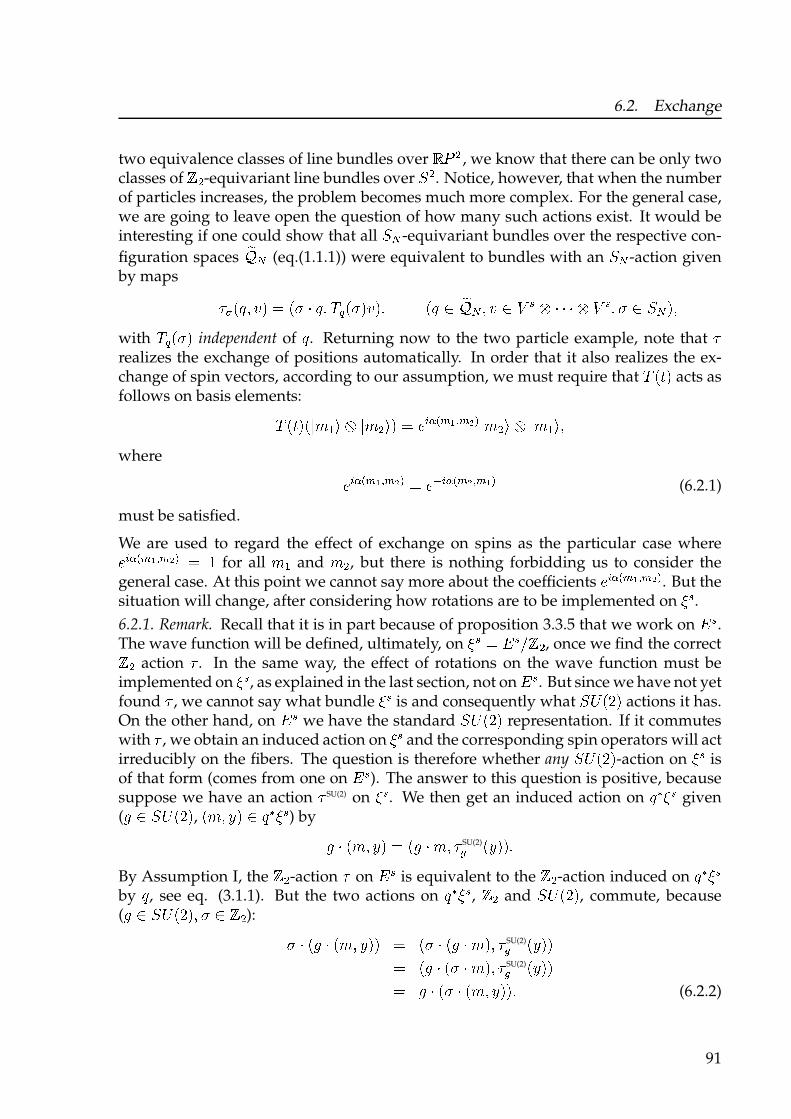
6.2. Exchange
two equivalence classes of line bundles over ¿ À Á , we know that there can be only twoclasses of  Á-equivariant line bundles over à Á . Notice, however, that when the numberof particles increases, the problem becomes much more complex. For the general case,we are going to leave open the question of how many such actions exist. It would beinteresting if one could show that all ÃÄ -equivariant bundles over the respective con-
figuration spaces ÅÆÄ (eq.(1.1.1)) were equivalent to bundles with an ÃÄ -action givenby maps ÇÈ ÉÊ Ë Ì Í Î ÉÏ Ð Ê Ë Ñ Ò ÉÏ ÍÌ ÍË ÉÊ Ó ÅÆÄ Ë Ì Ó Ô Õ Ö Ð Ð Ð Ö Ô Õ Ë Ï Ó ÃÄ ÍËwith
ÑÒ ÉÏ Íindependent of
Ê. Returning now to the two particle example, note that
Çrealizes the exchange of positions automatically. In order that it also realizes the ex-change of spin vectors, according to our assumption, we must require that
Ñ É× Íacts as
follows on basis elements:Ñ É× Í ÉØÙ ÚÛ Ö ØÙ Á ÛÍ Î ÜÝÞ ßà á âà ã ä ØÙ Á Û Ö ØÙ ÚÛ Ëwhere ÜÝÞ ßà á âà ã ä Î ÜåÝÞ ßà ã âà áä
(6.2.1)
must be satisfied.
We are used to regard the effect of exchange on spins as the particular case whereÜÝÞ ßà á âà ã ä Î æ
for all Ù Ú and Ù Á , but there is nothing forbidding us to consider thegeneral case. At this point we cannot say more about the coefficients
ÜÝÞ ßà á âà ã ä. But the
situation will change, after considering how rotations are to be implemented on ç Õ.
6.2.1. Remark. Recall that it is in part because of proposition 3.3.5 that we work on è Õ.
The wave function will be defined, ultimately, on ç Õ Î è ÕéÂÁ, once we find the correctÂÁ action
Ç. In the same way, the effect of rotations on the wave function must be
implemented on ç Õ, as explained in the last section, not on è Õ
. But since we have not yetfound
Ç, we cannot say what bundle ç Õ
is and consequently what à ê ÉëÍactions it has.
On the other hand, on è Õwe have the standard à ê ÉëÍ
representation. If it commuteswith
Ç, we obtain an induced action on ç Õ
and the corresponding spin operators will actirreducibly on the fibers. The question is therefore whether any à ê ÉëÍ
-action on ç Õis
of that form (comes from one on è Õ). The answer to this question is positive, because
suppose we have an action
ÇSU(2) on ç Õ
. We then get an induced action on
Ê ìç Õgiven
(í Ó Ã ê ÉëÍ,
ÉÙ Ë î Í Ó Ê ìç Õ) by í Ð ÉÙ Ë î Í Î Éí Ð Ù Ë Ç
SU(2)ï Éî ÍÍðBy Assumption I, the  Á-action
Çon è Õ
is equivalent to the ÂÁ-action induced on
Ê ìç Õby
Ê, see eq. (3.1.1). But the two actions on
Ê ìç Õ, ÂÁ and à ê ÉëÍ
, commute, because(í Ó Ã ê ÉëÍË Ï Ó Â Á): Ï Ð Éí Ð ÉÙ Ë î ÍÍ Î ÉÏ Ð Éí Ð Ù ÍË Ç
SU(2)ï Éî ÍÍÎ Éí Ð ÉÏ Ð Ù ÍË ÇSU(2)ï Éî ÍÍÎ í Ð ÉÏ Ð ÉÙ Ë î ÍÍð
(6.2.2)
91

6. Further developments
This means that ñ also commutes with the ò ó ôõö action on ÷ ø induced by ñ SU(2). Butthis last action is (we expect) induced by a representation of ò ó ôõö. Since the spin op-erators induced by ñ SU(2) act locally on the fibers as representations isomorphic to theusual ones on ù ø ú ù ø, we have arrived at the conclusion that ñ must commute with theusual ò ó ôõö representation on ÷ ø (i.e. on ù ø ú ù ø). Therefore, we make the following
Assumption II The ûü action ñ on ÷ ø must commute with ò ó ôõö.6.2.2. Proposition. Assumption II implies that all terms ýþÿ �� � �� � � are equal to a factor ô��ö� .
Proof. Let � � denote the vectors in the basis of total angular momentum. The re-
quirement that the actions commute implies that the corresponding representations com-mute: �� ô� ö � � �� � ô� ö� � � � � ô� � ûü � � � ò ó ôõöö �This is equivalent to requiring�� ô� ö � �þ� � � � � � � � �� õ � �for the infinitesimal generators. From (6.2.1), it follows that ýþÿ �ø �ø� � ô��ö� for someinteger � . Using õ � õ � ú we obtain, from
�� ô� ö � �!� õ � õ � �:� ô� ö õ � õ � � � �"# � ô� ö�! õ � õ � �"# �!� ô� ö õ � õ � ô��ö� õ � õ � � �
Applying� ô� ö to all vectors õ � $
, we obtain, in the same way as above,� ô� ö õ � $ � ô��ö� õ � $ � �õ % $ % õ �From this we obtain:ô��ö� õ � $ � � ô� ö &���� � ô � ' � � ü õ $ ö � ' ú � ü � &� � �� � ô � ' � � ü õ $ öýþÿ �� � �� � � � ü ú � '
� &� � �� � ô � ' � � ü õ $ öýþÿ �� � �� � � � ' ú � ü �Putting
$ � � ' ( � ü in the last equation, we obtain, using the linear independenceof the basis, ýþÿ �� � �� � � � ô��ö� . Note that in order to use linear independence it is
92
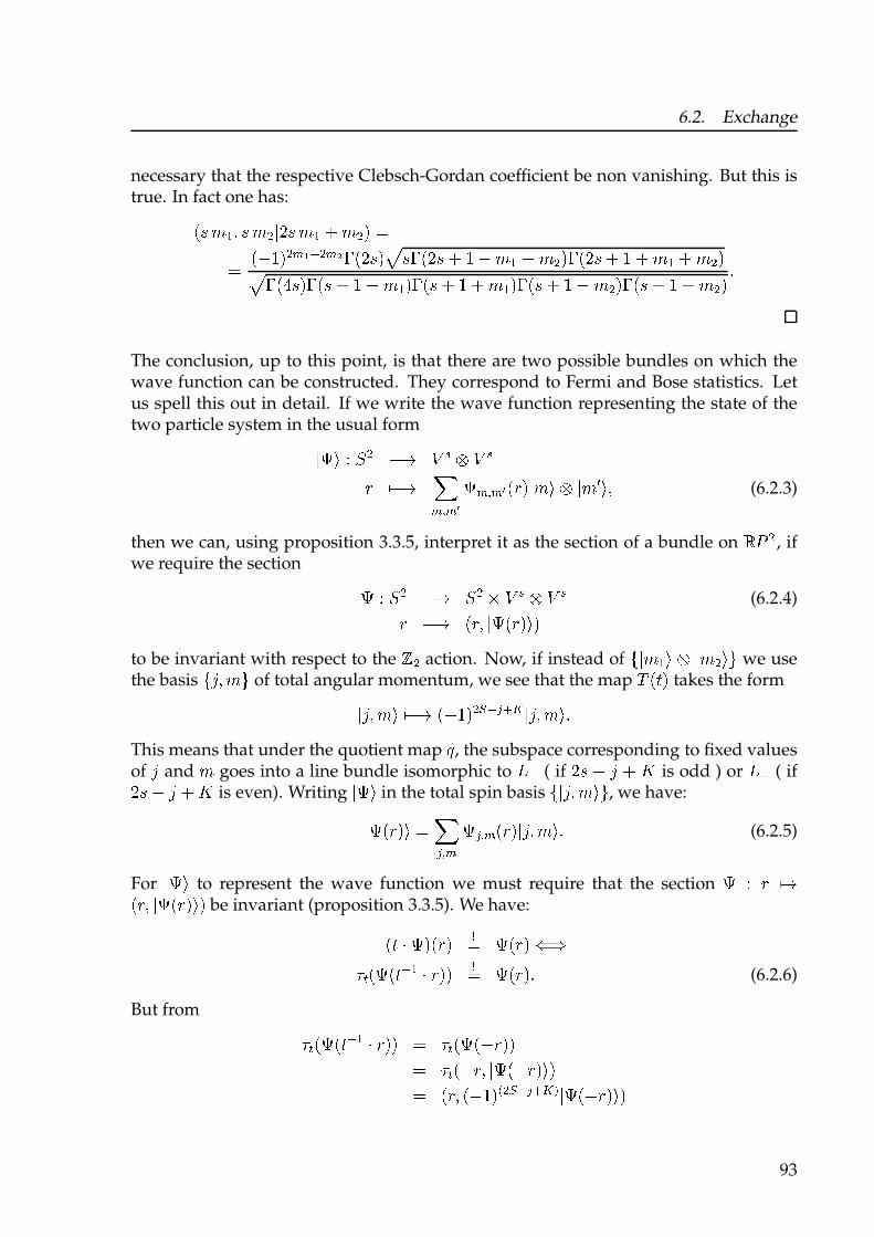
6.2. Exchange
necessary that the respective Clebsch-Gordan coefficient be non vanishing. But this istrue. In fact one has:)* + , - * + . /0* + , 1 + . 2 33 )452.6 78.6 9 : )0*2;*: )0* 1 5 4 + , 4 + . 2: )0* 1 5 1 + , 1 + . 2;: )<*2: )* 1 5 4 + ,2: )* 1 5 1 + ,2: )* 1 5 4 + . 2: )* 1 5 1 + . 2 =The conclusion, up to this point, is that there are two possible bundles on which thewave function can be constructed. They correspond to Fermi and Bose statistics. Letus spell this out in detail. If we write the wave function representing the state of thetwo particle system in the usual form/> ? @ A . 4B C D E C DF G4B H6 I6 J >6 I6 J )F 2 /+ ? E /+ K? -
(6.2.3)
then we can, using proposition 3.3.5, interpret it as the section of a bundle on L M ., if
we require the section > @ A . 4B A . N C D E C D(6.2.4)F G4B )F- /> )F 2?2
to be invariant with respect to the O.action. Now, if instead of P /+ ,? E /+ . ?Q
we usethe basis PR - + Q
of total angular momentum, we see that the map S )T 2takes the form/R - + ? G4B )452.U VW 8X /R - + ? =
This means that under the quotient map YZ , the subspace corresponding to fixed valuesof R and
+goes into a line bundle isomorphic to [V
( if0* 4 R 1 \
is odd ) or [8( if0* 4 R 1 \
is even). Writing/> ?
in the total spin basis P /R - + ?Q, we have:/> )F 2? 3 HW I6 >W I6 )F 2 /R - + ? = (6.2.5)
For/> ?
to represent the wave function we must require that the section> @ F GB)F- /> )F 2?2 be invariant (proposition 3.3.5). We have:)T ] > 2)F 2 3 > )F 2 _`ab )> )TV, ] F 22 3 > )F 2= (6.2.6)
But from ab )> )TV, ] F 22 3 ab )> )4F 223 ab )4F - /> )4F 2?23 )F - )4 52c.U VW 8X d /> )4F 2?293

6. Further developments
then we obtain, for the coefficient functions:ef ghijk lm no pqm rs eft h u qm rs et hv(6.2.7)
Transforming back to the w xy z{ | xy j {} basis, we get:qs~ rs � eft h u efghjkno qs � rs ~ et h � (6.2.8)
that is, the Fermi-Bose alternative. Let us finish this section with some remarks con-cerning this derivation.� As remarked above, for the case � � � case, the �� actions that we have consid-
ered are not the most general one can conceive. It would be interesting to findout how many possibilities there are, in order to be able to extend our argumentsto that general case.� The derivation of the Fermi-Bose alternative we have proposed is consistent withthe point of view we have adopted of working in a configuration space of in-distinguishable particles. The equivariance of the bundles over the covering ofthe configuration space play the double role of defining how to obtain the vectorbundle where the physical wave function is defined and at the same time real-izes exchange. Our first proposed assumption says that the action that realizesexchange must be precisely the one with respect to which the quotient is takenon the bundle.� As presented here, this derivation is specific to the two particle case, which is arestriction. But on the other hand, it works for any value of the spin.
94
A. G-Spaces
In this appendix we collect some standard facts about �-spaces. They are used inchapter 3.
A.1. Definition. A topological group is a group � which at the same time is a topologicalspace, such that the map � � � � ��� � � � �� � ���is continuous.
A.2. Definition (G-space). Let � be a topological group and � a topological space.A map � � � � � � � is called a (left-) group action when, for every � � � ,� �� � � � � � � �� � � �� � � �� ��� � � � � � and � �� � � � � � . If the map � is continuous, � issaid to be a left G-space. A right G-space is defined similarly.
A.3. Remark. It is usual to denote an action � in the following way: � �� �� � �� � � �. For� � � fixed, one considers the “partial map” �� , defined through�� � � � �� �� � � � � � �� � � ��A.4. Definition (G-Orbit). Let � be a left G-space. Given � � � , the set� � � � �� � � � � � � ¡ �is called the orbit of � and will be denoted ¢£ .
A.5. Definition (Free action). A group action is called free when �¤ � �� for all ¥ in� , i.e. when for all ¥ � � , � � ¥ � ¥ ¦ � � �holds.
A.6. Remark. Equivalently, one can say: A group action is free if and only if for every �in � § �� , the fixed-point set �¥ � � �� � ¥ � ¥ is the empty set.
Let � be a discrete group and � a topological space. If additionally � acts on � , onemay ask under what conditions does the quotient space � ¨� retain certain topolog-ical properties that � might posses. If, for instance, � ¨� is a Hausdorff space, then
95
A. G-Spaces
every point © ª « ¬ is a closed set. Since the canonical projection ® ¯ « ° « ¬ iscontinuous (by definition of the quotient topology), the set ® ±² ³© ´ must also be closedor, in other words, if © µ ® ³¶ ´, then the orbit ·¸ must be a closed set. It is clear that notevery group action satisfies this condition.
An interesting case is the one where « is a (differentiable) manifold. Under the as-sumption of a free and properly discontinuous action, it is possible to show that « ¬inherits the structure of a (differentiable) manifold. Since this well-known result[Boo02, BG88] will be needed several times in this work, a proof of it will be givenbelow. First we begin by explaining the term “properly-discontinuous”.
A.7. Definition (Properly discontinuous action). A properly discontinuous action of adiscrete group on a topological (resp. differentiable) manifold is a continuous (resp.differentiable) action such that:
(i) ¹¶ º » ª « :» ¼ª ·¸ ½ ¾ ¿ º À neighborhoods such that ¶ ª ¿ , » ª À and ³ Á ¿ ´  À µ Ã.
(ii) There is, for every ¶ ª « , a neighborhood ¿ such that the set ÄÅ ª Æ Å Á ¿  ¿ µÃÇ is finite.
A.8. Remark. The second condition may be replaced by the following, equivalent oneÈ(ii)’ For every ¶ ª « , the isotropy group ¸ ¯µ ÄÉ ª ÆÉ Á ¶ µ ¶ Ç is finite and there
is a neighborhood ¿ of ¶ such that ³É Á ¿ ´  ¿ µ à for É ¼ª ¸ and É Á ¿ µ ¿ forÉ ª ¸ .
A.9. Theorem. Let « be a topological (resp. differentiable) manifold and a discrete groupacting freely and properly-discontinuously on « . Then « ¬ inherits from « the structure ofa topological (resp. differentiable) manifold.
Proof. Set Ê µ dim³« ´. Give « ¬ the quotient topology, that is, the weakest topologysuch that the canonical projection ® ¯ « ° « ¬¶ Ë° ̶Íis continuous (or equivalently: Î is open in « ¬ Ï ®±² ³Î ´ is open in « ). We firstverify that « ¬ is a topological manifold. The following properties must be checked:Ð M/G is Hausdorff.Ð Every point in « ¬ has a neighborhood homeomorphic to Ñ Ò .Ð « ¬ admits a countable basis for its topology.Ó
See [Boo02]
96

The fact that Ô ÕÖ is Hausdorff is a direct consequence from (i) in definition A.7 ×. IfØ Ù Ô is open, then so is Ú Û Ø ÜÚ Ý Ö Þ. This follows from the continuity of theaction ß à Ö á Ô â Ô since, for fixed Ú Ý Ö , the partial map ßã à Ô â Ô is alsocontinuous and Ú Û Ø ä ßåæã çè ÜØ Þ. It follows that the union éãêë Ú Û Ø is also open.
From ì åæ Üì ÜØ ÞÞ ä éãêë Ú Û Ø and the definition of quotient topology it follows thatì ÜØ Þ is open, i.e., ì is an open map.
On the other hand, we know that Ô has a countable basis íîï ðïêñ (ò a countable indexset). Using the fact that ì is open, it is easy to show that íì Üîï Þðïêñ is a countable basisfor the topology of Ô ÕÖ . Indeed, let ó Ù Ô ÕÖ be an open set. Then we have:ì is continuous ô ìåæ Üó Þ open in Ô ôõö Ù ò with ì åæ Üó Þ ä ÷ø êù îø ô ó ä ì ú÷ø êù îø û ä ÷ø êù ì Üîø ÞüThe assertion follows since, for every ý , ì Üîø Þ is an open set (ì is an open map).
For every þ in Ô we have Öÿ ä í�ð, because the action is free. From (ii)’ it followsthat for every þ there is a neighborhood
�îÿ � þ withÜÚ Û �îÿ Þ � �îÿ ä �
for all Ú inÖ � í�ð. Putting î �ÿ � àä ì Ü �îÿ Þ, one obtains a bijective map ì � � à �îÿ â î �ÿ �. This map ismoreover a homeomorphism, since ì is open and continuous. We can assume, withoutloss of generality, that
�îÿ belongs to a chart í �îÿ � � ð. Then
àä � � Üì � � Þåæ à î �ÿ � â � Ü �îÿ Þ Ù � �is also a homeomorphism. This means (since ì is surjective) that Ô ÕÖ is a topologicalmanifold.
When Ô is, in addition, a differentiable manifold, it is possible to construct an atlasfor Ô ÕÖ in the following way. Let us denote the elements of Ö with Úï, � Ý � ë , where� ë Ù �
is an index set such that �� ë � ä �Ö �, � Ý � ë . Choose the indexing in such a waythat Ú æ ä � holds and set ßï Ü Û Þ àä ß ÜÚï � Û Þ.Now, it is convenient to choose charts íÜ �î� �ï � � � �ï Þð�ê� �ïê� � for Ô with the followingproperties:
� For � fixed,�î� �ï ä ßï Ü �î� �æ Þ (� Ý � ë).
� ßï Ü �î� �æ Þ � �î� �æ ä �(� Ý � ë � í�ð).
For such charts we then have, for all �:�î� �ï � �î� �ø ä � Ü� �ä ý Þ � (A.1)ì Ü �î� �ï Þ ä ì Ü �î� �ø Þ Ü� � � ý Þ ü�They are, in fact, equivalent assertions, see [Boo02].
97

A. G-Spaces
For this reason we may set �� ! " # $�� %& ', with ( ) * + arbitrarily chosen. It follows that
" ,- #�� ' ! .&/0 1 $�� %& ! .&/0 1 2& # $�� %- ' (A.2)
is a union of pairwise disjoint neighborhoods. With "� %& ! " 3 456 78 , we can now define
charts 9#�� : ;� '<�/0 (as before) by means of
; ! $;� %-=" ,-� %- �� >? $;� %- # $�� %- ' @ A B CLet D : E ) * be such that �� F �G H! I. Let JK L ) �� F �G and choose a representativeK ) �� %-. Then there is a unique ( ) * + with K ) �G %&, from which
;G =; ,-� ! $;G %-=2 ,-& = $; ,-� %-follows. Since the three maps on the right hand side of this equation are diffeomor-phisms, the transition function ;G =; ,-� is also a diffeomorphism.
A.10. Remark. Of course, from �� F �G H! I it does not follow, in general, that $�� %&F $�G %M H!I for arbitrary ( and N . But, if one chooses a certain (, a unique N ! N #(' is singled out, insuch a way that $�� %& F $�G %M H! I holds. Putting $2& ! $;� %& =2& = $; ,-� %-, we obtain the followingexpression for the transition functions:
;G =; ,-� ! # $;G %-=" ,-G %- '= # $;� %-=" ,-� %- ',- ! $;G %-= #" ,-G %-="� %- '= $; ,-� %- !! $;G %-= #2 ,-M =2& '= $; ,-� %- ! # $;G %-=2 ,-M '= #2& = $; ,-� %- ' ! (A.3)
! # $2 ,-M = $;G %M '= # $; ,-� %& = $2& ' !! $2 ,-M = # $;G %M = $; ,-� %& '= $2& C
The diagram below might help to keep track of the different maps involved in the con-struction:
A B $�� %&4O6 78 $�� %& F $�G %M $�G %M 4OP 7Q A B
A B4R8
$�� %-4O6 7S R8
T6 7SRUSQ =R8V
VTUSP 7S=T6 7S $�G %-RQ
4OP 7STP 7S A B
4RQ
��O6
�� F �G �GOP
(A.4)
A.11. Remark. When W is finite, it is enough to require that 2 be a free action in order toapply theorem A.9. In this case, the second condition in XA.7 is trivially satisfied. Thefirst one is also satisfied. To see this, let us first write W ! 9Y - : C C C : YZ < ([ ! 3W 3). Theorbit of K ) \ is the given by ]^ ! 9Y& _K <& . Let ` be in \ but with ` a) ]^ . Then ` H! Y& _K b ( ) 9c: C C C : [ <. Since \ is Hausdorff, we know that there are open neighborhoods�& d Y& _ K and e& d ` , for which �& F e& ! I holds. Defining � ! f Z&V - #Y ,-& _ �& ' ande ! f Z&V - e&, we thus get: � and e are open and #Y & _� 'F e g �& F e& ! I, ( ) 9c: C C C : [ <.From this it follows that #W _ � ' F e ! I, i.e. (i) from XA.7 holds.
98

Bibliography
[AB02] M. Atiyah and R. Bielawski, Nahm’s Equations, Configurations Spaces andFlag Manifolds, Bull. Brazilian Math. Soc., vol. 33, pp. 157–166, 2002.
[AM03] R.E. Allen and A.R. Mondragon, Comment on “Spin and statistics in nonrel-ativistic quantum mechanics: The spin-zero case”, Phys. Rev. A, vol. 68, pp.046101, 2003.
[Art47] E. Artin, Theory of braids, Ann. Math., vol. 48, pp. 101–126, 1947.
[Ati67] M.F. Atiyah, K-theory, Benjamin, New York, 1967.
[BDGh90] A.P. Balachandran, A. Daughton, Z.C. Gu, G. Marmo, R.D. Sorkin, andA.M. Srivastava, A topological spin-statistics theorem or a use of the antiparticle,Mod. Phys. Lett. A, vol. 5, pp. 1575–1585, 1990.
[BDGh93] A.P. Balachandran, A. Daughton, Z.C. Gu, R.D. Sorkin, G. Marmo, andA.M. Srivastava, Spin-statistics theorems without relativity or field theory, Int.J. Mod. Phys. A, vol. 8, pp. 2993–3044, 1993.
[Ber67] H. Bernstein, Spin precession during interferometry of fermions and the phasefactor associated with rotations through ij radians, Phys. Rev. Lett., vol. 18,pp. 1102–1103, 1967.
[Ber84] M.V. Berry, Quantal phase factors accompanying adiabatic changes, Proc. R.Soc. London A, vol. 392, pp. 45–57, 1984.
[BFFh78] F. Bayen, M. Flato, C. Fronsdal, A. Lichnerowicz, and D. Sternheimer, De-formation theory and quantization. I,II., Ann. Physics, vol. 111, pp. 61–151,1978.
[BG88] M. Berger and B. Gostiaux, Differential geometry: Manifolds, curves and sur-faces, Springer-Verlag, New York, 1988.
[BH50] F. Bopp and R. Haag, Uber die Moglichkeit von Spinmodellen, Z. Naturforsch,vol. 5a, pp. 644–653, 1950.
[BL81] L.C. Biedenharn and J.D. Louck, The Racah-Wigner Algebra in QuantumTheory, in G.C. Rota, editor, Encyclopedia of Mathematics and its Applications-Vol. 9. Addison-Wesley, 1981.
99
Bibliography
[Boo02] W.M. Boothby, An Introduction to Differentiable Manifolds and RiemannianGeometry, Revised, Academic Press, 2002.
[BR97] M.V. Berry and J.M. Robbins, Indistinguishability for quantum particles: spin,statistics and the geometric phase, Proc. R. Soc. London A, vol. 453, pp. 1771–1790, 1997.
[BR00] M.V. Berry and J.M. Robbins, Quantum indistinguishability: alternative con-structions of the transported basis, J. Phys. A, vol. 33, pp. L207–L214, 2000.
[DHR71] S. Doplicher, R. Haag, and J.E. Roberts, Local Observables and Particle Statis-tics I, Commun. Math. Phys., vol. 23, pp. 199–230, 1971.
[DHR74] S. Doplicher, R. Haag, and J.E. Roberts, Local Observables and Particle Statis-tics II, Commun. Math. Phys., vol. 35, pp. 49–85, 1974.
[DS97] I. Duck and E.C.G. Sudarshan, Pauli and the Spin-Statistics Theorem, WorldScientific, Singapore, 1997.
[Fed94] B. Fedosov, A simple geometrical construction of deformation quantization, J.Differential Geom., vol. 40, pp. 213–238, 1994.
[FH65] R. P. Feynman and A.R. Hibbs, Quantum Mechanics and Path Integrals,McGraw-Hill, 1965.
[Fie39] M. Fierz, On the Relativistic Theory of Force Free Particles of Arbitrary Spin,Helv. Phys. Acta, vol. 12, pp. 3–37, 1939.
[FR68] David Finkelstein and Julio Rubinstein, Connection between spin, statistics,and kinks, J. Math. Phys., vol. 9, pp. 1762–1779, 1968.
[GBVF01] J.M. Gracia-Bondıa, J.C. Varilly, and H. Figueroa, Elements of Noncommuta-tive Geometry, Birkhauser, 2001.
[GL95] D. Guido and R. Longo, An Algebraic Spin and Statistics Theorem, Commun.Math. Phys., vol. 172, pp. 517–534, 1995.
[HMS89] P.A. Horvathy, G. Morandi, and E.C.G. Sudarshan, Inequivalent Quantiza-tions in Multiply Connected Spaces, Il Nuovo Cimento, vol. 11D, pp. 201–228,1989.
[HPRS87] A. Heil, N.A. Papadopoulos, B. Reifenhauser, and F. Scheck, Scalar matterfield in a fixed point compactified five-dimensional Kaluza-Klein theory, Nucl.Phys. B, vol. 281, pp. 426–444, 87.
[HR04] J.M. Harrison and J.M. Robbins, Quantum indistinguishability from generalrepresentations of SU(2n), J. Math. Phys., vol. 45, pp. 1332–1358, 2004.
100

Bibliography
[Ish84] C. J. Isham, Topological and global aspects of quantum theory, in Bryce S. De-Witt and Raymond Stora, editors, Relativity, Groups and Topology II, Kluweracademic publishers, Amsterdam, pp. 1059–1290, 1984.
[Kat50] Tosio Kato, On the Adiabatic Theorem of Quantum Mechanics, Journal of thePhysical Society of Japan, vol. 5, pp. 435–439, 1950.
[Kuc04] B. Kuckert, Spin and Statistics in nonrelativistic Quantum Mechanics, I,Physics Letters A, vol. 322, pp. 47–53, 2004.
[Lan01] G. Landi, Projective modules of finite type and monopoles over k l , J. Geom.Phys., vol. 37, pp. 47–62, 2001.
[LD71] Michael G.G. Laidlaw and Cecile Morette DeWitt, Feynman functional inte-grals for systems of indistinguishable particles, Phys. Rev. D, vol. 3, pp. 1375–1378, 1971.
[LM77] J.M. Leinaas and J. Myrheim, On the theory of identical particles, Il NuovoCimento, vol. 37B, pp. 1–23, 1977.
[LZ58] G. Luders and B. Zumino, Connection between Spin and Statistics, Phys. Rev.,vol. 110, pp. 1450, 1958.
[Mer62] E. Merzbacher, Single Valuedness of Wavefunctions, Am. J. Phys., vol. 30, no.4, pp. 237–247, 1962.
[Mor92] G. Morandi, The Role of Topology in Classical and Quantum Physics (LectureNotes in Physics vol.m-7), Springer-Verlag, 1992.
[MS74] J.W. Milnor and J.D. Stasheff, Characteristic Classes, Princeton Univ. Press,Princeton, NJ, 1974.
[MT97] I. Madsen and J. Tornehave, From Calculus to Cohomology: De Rham coho-mology and characteristic classes, Cambridge Univ. Press, Cambridge, UK,1997.
[Pas01] M. Paschke, Von Nichtkommutativen Geometrien, ihren Symmetrien und et-was Hochenergiephysik, Dissertation, Institut fur Physik, Universitat Mainz,2001.
[Pau33] W. Pauli, Die allgemeinen Prinzipien der Wellenmechanik, H. Geiger andK. Scheel, editors, Handbuch der Physik, volume 24, part 1, Berlin, p. 126.
[Pau39] W. Pauli, Uber ein Kriterium fur Ein- oder Zweiwertigkeit der Eigenfunktionenin der Wellenmechanik, Helv. Phys. Acta, vol. 12, pp. 147–168, 1939.
[Pau40] W. Pauli, The Connection Between Spin and Statistics, Phys. Rev., vol. 58, pp.716–722, 1940.
101
Bibliography
[Pes03a] Murray Peshkin, Reply to Comment on Spin and statistics in nonrelativisticquantum mechanics: The spin-zero case, Phys. Rev. A, vol. 68, pp. 046102,2003.
[Pes03b] Murray Peshkin, Spin and statistic in nonrelativistic quantum mechanics: Thespin-zero case, Phys. Rev. A, vol. 67, pp. 042102, 2003.
[PPRS04] N.A. Papadopoulos, M. Paschke, A. Reyes, and F. Scheck, The Spin-Statistics relation in nonrelativistic Quantum Mechanics and Projective Modules,Annales Mathematiques Blaise-Pascal, vol. 11, no. 2, pp. 205–220, 2004.
[RB94] J.M. Robbins and M.V. Berry, A geometric phase for m n o spins, J. Phys. A,vol. 27, pp. L435–L438, 1994.
[Sch68] Lawrence Schulman, A Path Integral for Spin, Phys. Rev., vol. 5, pp. 1558–1569, 1968.
[Ser58] J.-P. Serre, Modules projectifs et espaces fibres a fibre vectorielle, SeminaireDubreil, vol. 23, 1957-58.
[Sim83] Barry Simon, Holonomy, the Quantum Adiabatic Theorem, and Berry’s Phase,Phys. Rev. Lett., vol. 51, pp. 2167–2170, 1983.
[Sou69] J.M. Souriau, Structure des Systemes Dynamiques, Dunod, Paris, 1969.
[SW00] R.F. Streater and A.S. Wightman, Spin, Statistics and all That, Princeton U.Press, Princeton, 2000.
[Swa62] R.G. Swan, Vector bundle and projective modules, Trans.Amer.Math.Soc., vol.105, pp. 264–277, 1962.
[Tsc89] R.D. Tscheuschner, Topological spin-statistics relation in quantum field theory,Int. J. Theor. Phys., vol. 28, pp. 1269–1310, 1989.
[Ver01] R. Verch, A spin-statistics theorem for quantum fields on curved spacetime man-ifolds in a generally covariant framework, Commun. Math. Phys., vol. 223, pp.261–288, 2001.
[WCOE75] S.A. Werner, R. Colella, A.W. Overhauser, and C.F. Eagen, Observation ofthe phase shift of a neutron due to precession in a magnetic field, Phys. Rev. Lett.,vol. 35, pp. 1053–1055, 1975.
[Wig00] A.S. Wightman, The spin-statistics connection: Some pedagogical remarks inresponse to Neuenschwander’s question, Electron. J. Diff. Eqns., vol. Conf.04,pp. 207–213, 2000.
[Wil82] Frank Wilczek, Magnetic Flux,Angular Momentum, and Statistics, Phys. Rev.Lett., vol. 48, pp. 1144–1146, 1982.
102
Bibliography
[Woo80] N. Woodhouse, Geometric Quantization, Clarendon Press, Oxford, 1980.
[WY75] T.T. Wu and C.N. Yang, Concept of nonintegrable phase factors and global for-mulation of gauge fields, Phys. Rev. D, vol. 12, pp. 3845–3857, 1975.
103