On the Formal Foundation

of Ant Programming

Universite Libre de Bruxelles

Faculte des Sciences Appliquees

IRIDIA, Institut de Recherches Interdisciplinaireset de Developpements en Intelligence Artificielle

Directeur de Memoire :

Prof. Marco Dorigo

Dissertation presentee par Mauro

Birattari en vue de l’obtention

du Diplome d’Etudes Approfondies

en Sciences Appliquees.

Annee academique 2000/2001

Abstract

This thesis develops the formal framework of ant programming with the goal of

gaining a deeper understanding on ant colony optimization, a heuristic method

for combinatorial optimization problems inspired by the foraging behavior of ants.

Indeed, ant programming allows a deeper insight into the general principles un-

derlying the use of an iterated Monte Carlo approach for the multi-stage solution

of a combinatorial optimization problem. Such an insight is intended to provide

the designer of algorithms with new categories, an expressive terminology, and

tools for dealing effectively with the peculiarities of the problem at hand.

Ant programming searches for the optimal policy of a multi-stage decision

problem to which the original combinatorial problem is reduced.

In order to describe ant programming, in this thesis we adopt on the one hand

concepts of optimal control, and on the other hand the ant metaphor suggested

by ant colony optimization. In this context, a critical analysis is given of no-

tions as state, representation, and sequential decision process under incomplete

information.

i

Acknowledgments

This thesis presents the current state of a research which I have conducted during

the last two years in collaboration with Gianni Di Caro and Marco Dorigo.

In particular, I credit Gianni with introducing me to Ant Colony Optimiza-

tion. Gianni and I shared since the very beginning a deep interest in this research.

Without the never-ending discussions we had in person, by e-mail, and on the

telephone, this work would have been simply impossible.

Marco, “Father of All Ants,” has been on the other hand the perfect supervisor

for this work. Fundamental has been his logistic and administrative support.

Invaluable were his advices concerning all aspects of my research and of my

scientific activity: I’ve sadly regretted not following a couple. . . But most of all I

want to acknowledge Marco for the value he kept adding to my research through

comments, discussions, and brainstorming sessions: Extremely knowledgeable on

ant algorithms and related topics, Marco really seemed taking a pleasure in diving

into the gory details of this work.

A large amount of the ideas discussed in this thesis were already contained in

a technical report co-authored with Gianni and Marco [4].

The concept of mental image in Aristotle and Thomas Aquinas, and more

in general in Ancient and Medieval epistemology has been deeply discussed with

Carlotta Piscopo. The precise meaning of the Ancient Greek term phantasma,

and a research of occurrences of this term in the original Greek and Latin texts

were provided by Scilla Goria.

Marco Saerens suggested a couple of interesting readings about Optimal Con-

trol and Dynamic Programming. Patrice Latinne offered his logistic support that

has been fundamental expecially in these very last days: “Merci et bonne m***e!”

Even if quite indirect, the contribution given by Gianluca Bontempi is sensible.

I had first the chance to have him as supervisor for my master thesis, and then

the honor to be his colleague. He is the guy who taught me the job.

I thank all the people that either read early versions of this work, or discussed

with me its content: Prof. Claudio Birattari, Gianluca Bontempi, Grzegorz Ciel-

niak, Tom Duckett, Li Jun, Bruno Marchal, Nicolas Meuleau, Alessandro Saf-

ii

iii

fiotti, Thomas Stutzle. The remarks by Bruno in a very early stage, and by

Nicolas more recently have been particularly interesting, and they had an impor-

tant impact on my work. I thank Nicolas for spotting an error, and for suggesting

significative improvements both of the conceptual content and of the clarity of

the exposition.

I thank Prof. Philippe Smets, Hugues Bersini, Marco Dorigo, and all members

of Iridia for the extremely stimulating environment they created. I wish here

also to salute and to thank Prof. Wolfgang Bibel, Thomas Stutzle, and all my

old and new friends at Intellektik. Finally, I express my best wishes to the

young researchers involved in the Metaheuristics Network including Matthijs den

Besten, Christian Blum, and Andrea Roli.

* * *

On a more personal level I wish to thank Gianni, Marco, Scilla, Gianluca, Lele,

Vittorio, Elena, Stella, Anna, Massimiliano, Charlotte, Greg, Patrice, Frank,

Nathanael, Le Musee du Cinema, La Brasserie a Vapeur, Cantillon, 3 Fonteinen,

Rockit, Antoine, Danae, Luca, Daria, Mamma, and Papa. . .

My work is dedicated to Vladimiro and Carlotta.

M.B.

Contents

Abstract i

Acknowledgments ii

Contents iv

1 Introduction 1

2 Discrete optimization, optimal control, and paths on a graph 4

2.1 Incremental construction of a solution for a discrete optimization

problem . . . . . . . . . . . . . . . . . . . . . . . . . . . . . . . . 5

2.2 Multistage decision processes and optimal control . . . . . . . . . 7

2.3 Paths on a graph . . . . . . . . . . . . . . . . . . . . . . . . . . . 10

3 Markov and non-Markov representations 13

3.1 The concept of state in control theory . . . . . . . . . . . . . . . . 13

3.2 Markov property and the concept of representation . . . . . . . . 15

3.3 Generating a representation: from the state to the phantasma . . 16

4 Ant programming 24

4.1 The three phases of ant programming . . . . . . . . . . . . . . . . 24

4.1.1 Monte Carlo generation of paths: The “forward” phase . . 25

4.1.2 Biasing the generation of paths: The “backward” and the

“merge” phases . . . . . . . . . . . . . . . . . . . . . . . . 27

4.2 The algorithm and the metaphor . . . . . . . . . . . . . . . . . . 30

5 Conclusions and future work 34

Bibliography 38

iv

Chapter 1

Introduction

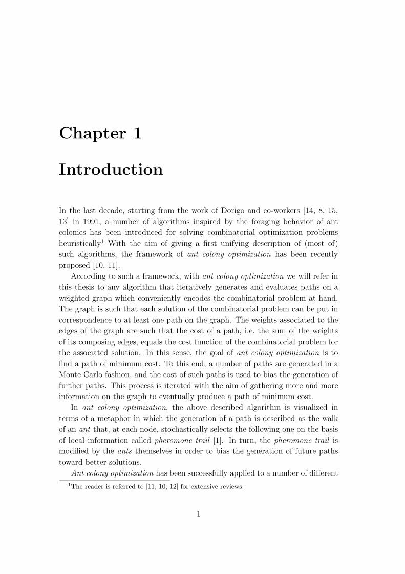
In the last decade, starting from the work of Dorigo and co-workers [14, 8, 15,

13] in 1991, a number of algorithms inspired by the foraging behavior of ant

colonies has been introduced for solving combinatorial optimization problems

heuristically1 With the aim of giving a first unifying description of (most of)

such algorithms, the framework of ant colony optimization has been recently

proposed [10, 11].

According to such a framework, with ant colony optimization we will refer in

this thesis to any algorithm that iteratively generates and evaluates paths on a

weighted graph which conveniently encodes the combinatorial problem at hand.

The graph is such that each solution of the combinatorial problem can be put in

correspondence to at least one path on the graph. The weights associated to the

edges of the graph are such that the cost of a path, i.e. the sum of the weights

of its composing edges, equals the cost function of the combinatorial problem for

the associated solution. In this sense, the goal of ant colony optimization is to

find a path of minimum cost. To this end, a number of paths are generated in a

Monte Carlo fashion, and the cost of such paths is used to bias the generation of

further paths. This process is iterated with the aim of gathering more and more

information on the graph to eventually produce a path of minimum cost.

In ant colony optimization, the above described algorithm is visualized in

terms of a metaphor in which the generation of a path is described as the walk

of an ant that, at each node, stochastically selects the following one on the basis

of local information called pheromone trail [1]. In turn, the pheromone trail is

modified by the ants themselves in order to bias the generation of future paths

toward better solutions.

Ant colony optimization has been successfully applied to a number of different

1The reader is referred to [11, 10, 12] for extensive reviews.

1

Chapter 1. Introduction 2

problems.2 Nevertheless, a complete theoretical analysis of the algorithms of this

class is not available yet.

The aim of this work is to produce a formal description of the combinatorial

optimization problems to which ant colony optimization applies, and to analyze

the implication of adopting a generic solution strategy based on the incremental

Monte Carlo construction of solutions. In particular, the thesis proposes a critical

analysis of the concept of state in the context of a sequential decision process.

Further, it introduces ant programming as an abstract class of algorithms which

presents all the characterizing features of ant colony optimization, but which is

more amenable to theoretical analysis. In particular, ant programming bridges

the terminological gap between ant colony optimization and the fields of optimal

control and reinforcement learning, with the final goal of exploiting the under-

standing gained in those fields for the analysis of ant colony optimization.

The name ant programming has been chosen for its assonance with dynamic

programming, with which ant programming has in common the idea of reformulat-

ing an optimization problem as a multi-stage decision problem. Both in dynamic

programming and in ant programming, such a reformulation is not a trivial one

and requires an ad hoc analysis of the optimization problem under consideration.

Once the multi-stage decision problem is defined, in ant programming as in dy-

namic programming, the optimal solution of the original optimization problem

can be generated through the optimal policy of the multi-stage decision problem.

These concepts, being among the main issues in this research, will be discussed

in detail in the rest of the thesis.

In Chapter 2 we show how the generic problem of discrete optimization with

a finite number of solutions can be described in terms of a discrete-time optimal

control problem which, in turn, can be mapped on the problem of searching the

path of minimal cost on a conveniently defined weighted graph.

Chapter 3 introduces the concepts of graph of the representation and of phan-

tasma. These concepts, which are related to the notion of sequential decision

process under incomplete information, will play a major role in the definition of

ant programming.

In Chapter 4 the ant programming abstract class of algorithms is introduced

and discussed. Moreover, a well defined semantic is given to all the elements of

the ant metaphor.

2The interested reader can found in [10, 12, 11] lists and descriptions of implementations

of ant colony optimization for a variety of combinatorial optimization problems like, among

others, traveling salesman, quadratic assignment, and graph coloring. Additionally, overviews

of algorithms inspired by the behavior of real ants but not strictly falling in the ant colony

optimization class, are reported in [6, 7, 9].

Chapter 1. Introduction 3

Chapter 5 describes the future developments of our research, and comments on

the significance of ant programming as a basis for providing ant colony optimiza-

tion with a new formal definition and a theoretical explanation. In particular, we

briefly introduce here two instances of ant programming, namely: Markov ants

and Marco’s ants. On the one hand, as it will be made clear in the body of the

thesis, the Markov ants algorithm is mainly of speculative interest, and is to be

considered as the extreme end of the ant programming class when the above men-

tioned sequential decision process is carried out under complete information. On

the other hand, the Marco’s ants algorithm is of much greater practical interest

and happens to present the characterizing features of the implementations of ant

colony optimization proposed so far in the literature, starting from the original

ant system introduced by Marco Dorigo et al., back in 1991 [14, 8].

Chapter 2

Discrete optimization, optimal

control, and paths on a graph

Let us consider a discrete optimization problem described by a finite set S of

feasible solutions, and by a cost function J defined on such a set.

The set S of feasible solutions is defined as

S = {s1, s2, . . . , sN}, N ∈ N, N < ∞, (2.1)

where each solution si is a ni-tuple

si = (s0i , s

2i , . . . , s

ni−1i ), ni ∈ N, ni ≤ n < ∞, (2.2)

with n = max ni, and sji ∈ Y , where Y is a finite set of components.

The cost function J : S → R assigns a cost to each feasible solution si. The

optimization problem is therefore the problem of finding the element s ∈ S which

minimizes the function J :

s = arg mins∈S

J(s), (2.3)

where with “arg min” we denote the element of the set S for which the minimum

is attained.1

Example: Let us consider a simple instance of the classical Trav-

eling Salesman Problem (TSP) [19, 20]. Here and in the following

examples, we consider a problem in which four cities are connected

to each other, and the distance between any two cities is the same

in either direction. The task is to find the shortest tour for visiting

1 Being the set S finite, the minimum of J on S indeed exists. If such minimum is attained

for more than one element of S, it is a matter of indifference which one is considered.

4

Chapter 2. Discrete optimization, optimal control, and paths on a graph 5

all the cities once and going back to the initial one, without passing

more than once by the same city.

If the cities are numbered from 1 to 4, it result that the set of the

components is

Y = {1, 2, 3, 4},

and the possible solution are all the sequences of four cities in which

none of the cities appears more than once:

S = {(1, 2, 3, 4), (1, 2, 4, 3), (1, 3, 2, 4), . . . , (4, 3, 2, 1)}.

In this particular example, all the solutions are composed by the same

number of elements: n = 4. The first solution, in a lexicographical

order, is here the solution s1 = (1, 2, 3, 4) that corresponds to the tour

starting from city 1 and visiting then cities 2, 3, and 4 in this order,

before terminating again in city 1.

The cost function J is the function that assigns to each solution si ∈ S

a real number measuring the length of the corresponding tour.

The remaining of this chapter will be devoted to give a formal description of the

process of incremental construction of solutions to problem 2.3.

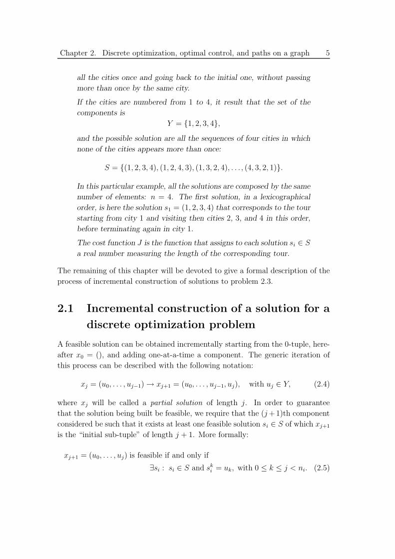
2.1 Incremental construction of a solution for a

discrete optimization problem

A feasible solution can be obtained incrementally starting from the 0-tuple, here-

after x0 = (), and adding one-at-a-time a component. The generic iteration of

this process can be described with the following notation:

xj = (u0, . . . , uj−1) → xj+1 = (u0, . . . , uj−1, uj), with uj ∈ Y, (2.4)

where xj will be called a partial solution of length j. In order to guarantee

that the solution being built be feasible, we require that the (j +1)th component

considered be such that it exists at least one feasible solution si ∈ S of which xj+1

is the “initial sub-tuple” of length j + 1. More formally:

xj+1 = (u0, . . . , uj) is feasible if and only if

∃si : si ∈ S and ski = uk, with 0 ≤ k ≤ j < ni. (2.5)

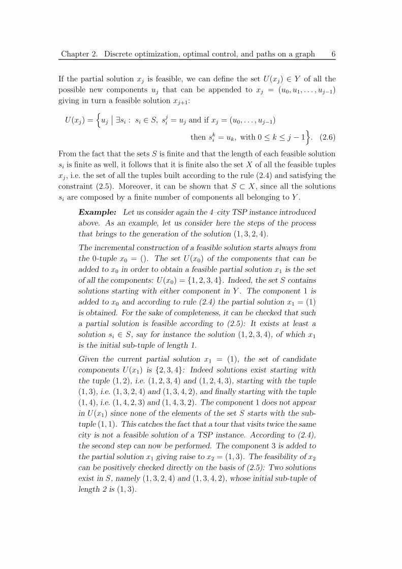
Chapter 2. Discrete optimization, optimal control, and paths on a graph 6

If the partial solution xj is feasible, we can define the set U(xj) ∈ Y of all the

possible new components uj that can be appended to xj = (u0, u1, . . . , uj−1)

giving in turn a feasible solution xj+1:

U(xj) ={

uj

∣

∣ ∃si : si ∈ S, sji = uj and if xj = (u0, . . . , uj−1)

then ski = uk, with 0 ≤ k ≤ j − 1

}

. (2.6)

From the fact that the sets S is finite and that the length of each feasible solution

si is finite as well, it follows that it is finite also the set X of all the feasible tuples

xj, i.e. the set of all the tuples built according to the rule (2.4) and satisfying the

constraint (2.5). Moreover, it can be shown that S ⊂ X, since all the solutions

si are composed by a finite number of components all belonging to Y .

Example: Let us consider again the 4–city TSP instance introduced

above. As an example, let us consider here the steps of the process

that brings to the generation of the solution (1, 3, 2, 4).

The incremental construction of a feasible solution starts always from

the 0-tuple x0 = (). The set U(x0) of the components that can be

added to x0 in order to obtain a feasible partial solution x1 is the set

of all the components: U(x0) = {1, 2, 3, 4}. Indeed, the set S contains

solutions starting with either component in Y . The component 1 is

added to x0 and according to rule (2.4) the partial solution x1 = (1)

is obtained. For the sake of completeness, it can be checked that such

a partial solution is feasible according to (2.5): It exists at least a

solution si ∈ S, say for instance the solution (1, 2, 3, 4), of which x1

is the initial sub-tuple of length 1.

Given the current partial solution x1 = (1), the set of candidate

components U(x1) is {2, 3, 4}: Indeed solutions exist starting with

the tuple (1, 2), i.e. (1, 2, 3, 4) and (1, 2, 4, 3), starting with the tuple

(1, 3), i.e. (1, 3, 2, 4) and (1, 3, 4, 2), and finally starting with the tuple

(1, 4), i.e. (1, 4, 2, 3) and (1, 4, 3, 2). The component 1 does not appear

in U(x1) since none of the elements of the set S starts with the sub-

tuple (1, 1). This catches the fact that a tour that visits twice the same

city is not a feasible solution of a TSP instance. According to (2.4),

the second step can now be performed. The component 3 is added to

the partial solution x1 giving raise to x2 = (1, 3). The feasibility of x2

can be positively checked directly on the basis of (2.5): Two solutions

exist in S, namely (1, 3, 2, 4) and (1, 3, 4, 2), whose initial sub-tuple of

length 2 is (1, 3).

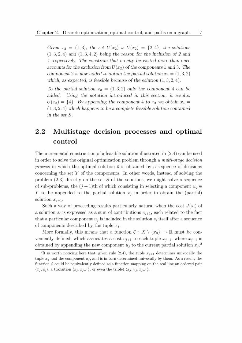
Chapter 2. Discrete optimization, optimal control, and paths on a graph 7

Given x2 = (1, 3), the set U(x2) is U(x2) = {2, 4}, the solutions

(1, 3, 2, 4) and (1, 3, 4, 2) being the reason for the inclusion of 2 and

4 respectively. The constrain that no city be visited more than once

accounts for the exclusion from U(x2) of the components 1 and 3. The

component 2 is now added to obtain the partial solution x3 = (1, 3, 2)

which, as expected, is feasible because of the solution (1, 3, 2, 4).

To the partial solution x3 = (1, 3, 2) only the component 4 can be

added. Using the notation introduced in this section, it results:

U(x3) = {4}. By appending the component 4 to x3 we obtain x4 =

(1, 3, 2, 4) which happens to be a complete feasible solution contained

in the set S.

2.2 Multistage decision processes and optimal

control

The incremental construction of a feasible solution illustrated in (2.4) can be used

in order to solve the original optimization problem through a multi-stage decision

process in which the optimal solution s is obtained by a sequence of decisions

concerning the set Y of the components. In other words, instead of solving the

problem (2.3) directly on the set S of the solutions, we might solve a sequence

of sub-problems, the (j + 1)th of which consisting in selecting a component uj ∈

Y to be appended to the partial solution xj in order to obtain the (partial)

solution xj+1.

Such a way of proceeding results particularly natural when the cost J(si) of

a solution si is expressed as a sum of contributions cj+1, each related to the fact

that a particular component uj is included in the solution si itself after a sequence

of components described by the tuple xj.

More formally, this means that a function C : X \ {x0} → R must be con-

veniently defined, which associates a cost cj+1 to each tuple xj+1, where xj+1 is

obtained by appending the new component uj to the current partial solution xj.2

2It is worth noticing here that, given rule (2.4), the tuple xj+1 determines univocally the

tuple xj and the component uj , and is in turn determined univocally by them. As a result, the

function C could be equivalently defined as a function mapping on the real line an ordered pair

〈xj , uj〉, a transition 〈xj , xj+1〉, or even the triplet 〈xj , uj , xj+1〉.

Chapter 2. Discrete optimization, optimal control, and paths on a graph 8

The function C must be such that

J(si) =

ni∑

j=1

cj, with cj = C(xj),

and where xj = (u0, . . . , uj−1),

with uk = ski for 0 ≤ k ≤ j − 1. (2.7)

Although a function C satisfying (2.7) can always be trivially obtained by im-

posing C(xj) = J(si), if ∃si ∈ S : xj = si, and C(xj) = 0 otherwise, we suppose

here that a non-trivial definition exists, and that its formulation is somewhat

“natural” for the problem at hand.

Example: In the case of our 4–city TSP, the function J associates

to every solution in S a cost which is the length of the corresponding

tour. It is quite natural to see this cost as the sum of the distances di-

viding the cities composing the tour. The function C can be naturally

defined as follows.

1. For any x1 = (u0) we put C(x1) = 0. This means that the cost

of starting from any city is always null.

2. For any feasible x2 = (u0, u1), we define that C assigns to x2 the

distance from the city u0 to the city u1.

3. For any feasible x3 = (u0, u1, u2), we define that C assigns to x3

the distance from the city u1 to the city u2.

4. For any feasible x4 = (u0, u1, u2, u3) we define that C assigns to

x4 the distance from the city u2 to the city u3 plus the distance

from the city u3 to the initial city u0.

The first case states that the cost of starting from any city is null. The

second and third are presented as distinct for clarity but both state

the basic fact that the function C is related to the distance between

the last two cities of the partial solution. The last case, together with

the distance between the last two cities, takes into account also the

distance to run in order to close the tour and go back to the initial

city.

The finite-horizon multi-stage decision process described above can be thoroughly

seen as a discrete-time optimal control problem [5].

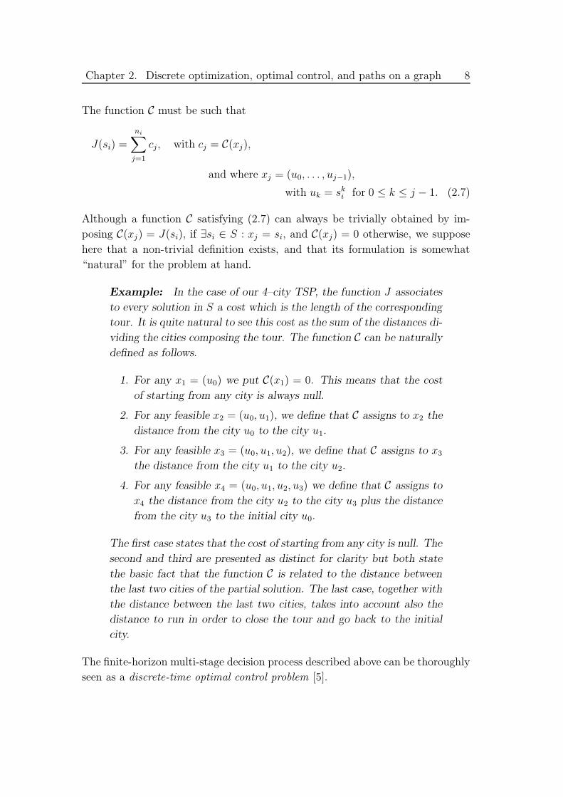
Chapter 2. Discrete optimization, optimal control, and paths on a graph 9

The tuple xj can be seen as the state at time t = j of the following discrete-

time dynamic system:{

xt+1 = F (xt, ut),

yt+1 = G(xt+1),(2.8)

with t ∈ N, xt, xt+1 ∈ X, where X is the set of the states of the system, yt+1 ∈ Y ,

where Y is the range of the output, and ut ∈ U(xt) where U(xt) is the set of the

control actions which are admissible when the system is in state xt.

Such a process is always started from the same initial state x0, and is termi-

nated when the state belongs to the set S ⊂ X, defined as the set of the final

states of the control process.

The state-transition application F : X × U → X is such that the state at

time t + 1 is obtained by “appending” the current control action ut ∈ U(xt) to

the state xt. Further, the function G : X → Y is such that the new component is

observed as the output at time t+1 of the system itself. Therefore, the following

notation will be adopted:{

xt+1 = [xt, ut],

yt+1 = ut,(2.9)

It results therefore that the set of the feasible actions, given the current state, is

a subset of the range of the output: U(xt) ⊂ Y .

Let now U be the set of all the admissible control sequences which bring the

system from the initial state x0 to a terminal state. The generic element of U ,

u = 〈u0, u1, . . . , uτ−1〉,

is such that the corresponding state trajectory, which is unique, is

〈x0, x1, . . . , xτ 〉,

with xτ ∈ S, and ut ∈ U(xt), for 0 ≤ t < τ . In this sense, the dynamic system

defines a mapping S : U → S which assigns to each admissible control sequence

u ∈ U a final state s = S(u) ∈ S.

The problem of optimal control consists in finding the sequence u ∈ U for

which the sum J of the costs ct, incurred along the state trajectory, is minimized:

u = arg minu∈U

J(

S(u))

, (2.10)

where with “arg min” we denote the element of the set U for which the minimum

of the composed function J ◦ S is attained.3

3The same remarks as in Note 1 apply here. Since the set U is finite, it is guaranteed that

J ◦ S attains its minimum on U .

Chapter 2. Discrete optimization, optimal control, and paths on a graph 10

2.3 Paths on a graph

It is apparent that the solution of the problem of optimal control stated in (2.10) is

equivalent to the solution of the original optimization problem (2.3), and that the

optimal sequence of control actions u for the optimal control problem determines

univocally the optimal solution s of the original optimization problem.

Since the set X is discrete and finite, together with all the sets U(xt), for all

xt ∈ X, and since trajectories have a fixed maximum length n, all the possible

state trajectories of the system (2.8) can be conveniently represented through a

weighted and oriented graph with a finite number of nodes.4

Let G(X, U, C) be such a graph, where X is the set of nodes, U is the set of

edges, and C is a function that associates a weight to each edge. In terms of the

system (2.8), the notation adopted means that each node of the graph G(X, U, C)

represents a state xt of the system. The set U ⊂ X × X is the set of the edges

〈xt, xt+1〉. Each of the edges departing from a given node xt represents one of the

actions ut ∈ U(xt) feasible when the system is in state xt. Therefore,

U =⋃

xt∈X

U(xt).

Finally, C : U → R is a function that associates a cost to every edge. Such a

function is defined in terms of the function C, and it results that

ct+1 = C(〈xt, xt+1〉) = C(xt+1)

is the cost of the edge 〈xt, xt+1〉.

Furthermore, on such a graph G(X, U, C) it can be singled out the initial

state x0, as the only state with no incoming edges, and the set S of the terminal

nodes from which no edges depart.

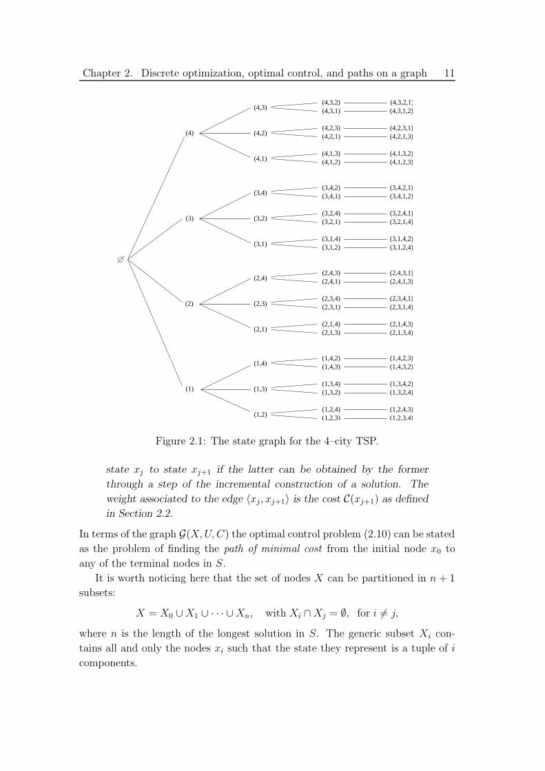
Example: The graph G(X, U, C) for the 4–city TSP is given in

Figure 2.1. The nodes of the graph are the possible states. The

terminal nodes, on the right side of the figure, are states encoding

solutions of the original optimization problem. An edge connects

4Remark on the notation adopted: Parenthesis (. . . ) are used for tuples of components

indicating the state of the system (2.8) or more in general a (partial) solution of the optimization

problem (2.3). Angle brackets 〈. . . 〉 are used for generic tuples: e.g., an edge of a graph

is represented as a pair 〈xt, xt+1〉 of nodes. Square brackets [·, ·] indicates the operation of

appending an element to a tuple: if xt is a tuple of length t, xt+1 = [xt, ut] is a tuple of

length t + 1 obtained by appending ut to xt. Braces {. . . } are used, as usual, for denoting a

set.

Chapter 2. Discrete optimization, optimal control, and paths on a graph 11

(4,3)

(4,2)

(4,1)

(3,4)

(3,2)

(3,1)

(2,4)

(2,3)

(2,1)

(1,4)

(1,3)

(1,2)

(4,3,1,2)(4,3,2,1)

(2)

(1)

(4)(4,2,3,1)(4,2,1,3)

(4,1,3,2)(4,1,2,3)

(3,4,2,1)(3,4,1,2)

(3,2,4,1)(3,2,1,4)

(3,1,4,2)(3,1,2,4)

(2,4,3,1)(2,4,1,3)

(2,3,4,1)(2,3,1,4)

(2,1,4,3)(2,1,3,4)

(1,4,2,3)(1,4,3,2)

(1,3,4,2)(1,3,2,4)

(1,2,4,3)(1,2,3,4)

(3)

(4,3,2)(4,3,1)

(4,2,3)(4,2,1)

(4,1,2)(4,1,3)

(3,4,1)(3,4,2)

(3,2,1)(3,2,4)

(3,1,2)(3,1,4)

(2,4,1)(2,4,3)

(2,3,1)(2,3,4)

(2,1,3)(2,1,4)

(1,4,3)(1,4,2)

(1,3,2)(1,3,4)

(1,2,3)(1,2,4)

Figure 2.1: The state graph for the 4–city TSP.

state xj to state xj+1 if the latter can be obtained by the former

through a step of the incremental construction of a solution. The

weight associated to the edge 〈xj, xj+1〉 is the cost C(xj+1) as defined

in Section 2.2.

In terms of the graph G(X, U, C) the optimal control problem (2.10) can be stated

as the problem of finding the path of minimal cost from the initial node x0 to

any of the terminal nodes in S.

It is worth noticing here that the set of nodes X can be partitioned in n + 1

subsets:

X = X0 ∪ X1 ∪ · · · ∪ Xn, with Xi ∩ Xj = ∅, for i 6= j,

where n is the length of the longest solution in S. The generic subset Xi con-

tains all and only the nodes xi such that the state they represent is a tuple of i

components.

Chapter 2. Discrete optimization, optimal control, and paths on a graph 12

As a consequence of the definition of the state-transition application F , the

edges departing from a non-terminal node xi ∈ Xi, enter a node xi+1 ∈ Xi+1. The

graph G(X, U, C) is therefore “sequential” and accordingly enjoys the property,

remarkable in this context, of being acyclic.

As already mentioned in Chapter 1, the solution strategy of ant colony opti-

mization is based on the iterated generation of multiple paths on a graph that

encodes the optimization problem under consideration. As it will be defined in

the following, this graph is obtained as a “transformation” of the graph G that

results being an aggregation of nodes of the latter. In previous works on ant

colony optimization, the graph resulting from such transformation was the only

graph taken into consideration explicitly. In this thesis, we move the focus on

the original graph G and on the properties of the transformation.

The importance of the graph G is related to the fact that it brings all the

information relevant for a multi-stage solution of the optimization task, as it is

carried out in ant colony optimization. More generally, the concepts and the

terminology peculiar to control theory and to the multi-stage solution of the

original optimization problem (2.3), holds fundamental importance in our analysis

of ant colony optimization, and constitutes the starting point for our discussion

on ant programming. In particular, in the following we will adopt the language

and the notation of control theory and we will focus on the analysis of concepts

like those of state and policy which are clearly defined in optimal control and

dynamic programming.

Before going to the core of these topics in the next chapters, it is worth to give

a more defined characterization of the class of “real” problems that ant colony

optimization is meant to deal with. As previously sketched, these algorithms look

for minimum cost paths on a graph. Being minimum cost path problems of great

practical and theoretical interest, a large number of heuristic or exact algorithms

has been proposed for their solution. The approach proposed in this thesis is

not to be considered as a general alternative to algorithms based on the “classic”

label setting techniques (e.g. Dijkstra algorithm) and label correcting techniques

(e.g. Bellman-Ford algorithm). On the contrary, it is intended to be used when

the dimension of the graph G overwhelm the available computational resources

as, for example, in large instances of NP-hard problems.

Chapter 3

Markov and non-Markov

representations:

The state and its phantasma

According to the parlance of optimal control, we have called a state each node

of the graph G(X, U, C) and, by extension, we use the expression state graph for

the graph G itself. In the following sections, the properties of the state graph will

be analyzed and discussed in the perspective of the solution of the problem (2.3),

and in relation to the solution strategy of ant colony optimization. The ant

metaphor introduced by ant colony optimization will be used as a visual tool

to make abstract concepts more clear. In particular, we will picture the state

evolution of the system (2.9), and therefore the incremental construction of a

solution as the walk of an ant on the state graph G. Accordingly, in the following

the state xt at time t will be called interchangeably the “partial solution,” the

“state of the system,” or, by extension, the “state of the ant.”

3.1 The concept of state in control theory

Informally, the state of a dynamic system can be thought of as the piece of

information that “completely” describes the system at a given time instant.

In more precise terms, for a deterministic discrete-time dynamic system, as

the one introduced in Eq. 2.8, the state is a tag or label that can be associated

to a particular aggregate of input-output histories of a system, and that enjoys

the following properties:

• At a given instant, the set of the admissible input sequences can be given

in terms of the state at that instant;

13

Chapter 3. Markov and non-Markov representations 14

• For all the admissible future input sequences, the state and a given admis-

sible input sequence determine univocally the future output trajectory.

It is very important that the reader be convinced of the relevance of both the

above stated properties. The following argumentation might help clarifying. Let

us say that, after being fed with a certain input sequence and having returned a

corresponding output sequence, the system at hand is left in a certain condition.

Given that the system is deterministic, for any possible continuation of the input,

the output will be univocally determined. Now, we say that two given conditions

are equivalent and are to be described by one and the same state, if they are

indistinguishable to a class of experiments defined as follows. We consider the

experiments that consist in feeding the system in the two different conditions with

the same input sequence, and we will say that the two conditions are indistin-

guishable to the given input sequence if the two corresponding output sequences

are equal. Therefore, the two conditions are to be labeled with the same state

if and only if they react with the same output sequence to any possible input

sequence. The two above stated properties follow directly. In particular, we want

to stress here the importance of the first one: If there exists an input sequence

that is admissible for one of the two conditions and not for the other, such an

input sequence is an experiment that enables us to distinguish the two conditions

that therefore cannot be labeled with the same state. Hence it is clear that, in

order for the two conditions to be equivalents and to be described with one and

the same state, it is necessary that they have the same set of admissible inputs.

In other words, all the conditions represented by the same state share the same

admissible inputs. Therefore the set of the admissible inputs is a property of each

state, i.e. such a set can be expressed as a function of the state, as indeed stated

by the first of the two properties.

The definition of state given here is inspired by and is consistent with the

classical definition given by Zadeh and Desoer [24]. It is nonetheless a proper

extension of that definition in the sense that we consider here systems for which

the set of admissible inputs varies according to the preceding input-output history,

while Zadeh and Desoer considered systems that always accept input in the same

given range. In this sense, our definition of state directly corresponds to the one

implicitly assumed in the literature on dynamic programming [2, 3].

Even if this thesis focuses on deterministic systems, another class of dynamic

systems, known as stochastic dynamic systems, is of particular interest. In a

stochastic dynamic system, the output at time t + 1 cannot be expressed deter-

ministically as a function of the state and of the input at time t and, at most,

some probability distribution can be given on its possible values. In general,

Chapter 3. Markov and non-Markov representations 15

a stochastic dynamic system can be obtained from a deterministic one if some

state components of the deterministic system are not available or are purposely

not taken into consideration.

Also in the case of a stochastic dynamic system, a definition of a state can be

given. In the stochastic case, instead of determining univocally the future output

trajectory, the state determines the probabilistic distribution of the future output,

and is such that past values of the states and of the input would not change the

probabilistic distribution if used to extend the state itself.

In more precise terms, xt is the state of the stochastic system at time t if it

determines the set U(xt) of the admissible control, and

Pk(yt+k|u, xt) = Pk(yt+k|u, xt, ut−1, xt−1, . . . , ut−m, xt−m),

for all k > 0, m > 0,

and for all admissible u = 〈ut, . . . , ut+k−1〉. (3.1)

By extension, a law of evolution of the state can be given only stochastically, and

the state at time t + 1 is a random variable whose value is extracted according

to the distribution P (xt+1|ut, xt) where again

P (xt+1|ut, xt) = P (xt+1|ut, xt, ut−1, xt−1, . . . , ut−m, xt−m),

for all m > 0, and for all ut ∈ U(xt). (3.2)

For the class of systems considered in this thesis, it is worth noticing that the

definition of state given above for the stochastic system, indeed encompasses the

one given for the deterministic system. In fact, in order to consider a deterministic

system, it is sufficient to define the distribution (3.2) so that the probability of

xt+1 conditioned to xt and ut, equals 1 if and only if, according to the deterministic

system (2.8), xt+1 follows xt when the input ut is applied.

As a consequence, both in the deterministic and in the stochastic case, we

can informally think of the state as the “most predictive” description that can

be given of the system.

3.2 Markov property and the concept of repre-

sentation

Since what is known in the literature as Markov property is related precisely to

the above stated definition of state, it is clear that the state, when correctly

conceived, is always a state in the Markov sense: When described in terms of

Chapter 3. Markov and non-Markov representations 16

its state, any discrete-time system1 is intrinsically Markov in the precise sense

given above. It is therefore of dubious utility to state the Markov property with

respect to a dynamic system tout court.

Of much greater significance, it is to assert the Markov property of a rep-

resentation. Informally, we call a representation the information on the system

that is available to an agent,2 and that is used in order to perform a prediction

or to select a control action.

In the limit, a representation might bear the same information as the state.

In this case we speak of a Markov representation or, equivalently, we say that

the Markov property holds for such representation. These expressions are to

be understood as an assertion of the fact that the representation considered is

equivalent to a state description of the system. In the more general case, a

representation gives “less information” than the state. Consistently, in this case

we say that the representation is of non-Markov type.

Being non-Markov is therefore a characteristic of the interaction system-agent

and is related to the fact that the agent describes the system in terms of an “in-

complete” representation. In general, such a shortcoming of the representation

can be ascribed to the inability of the agent to obtain information on the sys-

tem, or to the deliberate choice of reducing the amount of information to be

handled. In this second case, we can speak of a trade-off between the “quality”

of a description, and its “complexity.”

3.3 Generating a representation: from the state

to the phantasma

For the class of problems discussed in this thesis and generally described by

Eq. 2.3, a formal definition of a representation can be given, which refers directly

to the definition given above of the state graph G(X, U, C). Consistently with

that definition, we define the representation graph as the graph Gr(Zr, Ur, T ),

where Zr is the set of the nodes, and Ur is the set of the edges. The meaning and

usage of the function T : Ur → R will be made clear in the following.

Furthermore, we call generating function of the representation the function

r : X → Zr that maps the set X of the states onto the set Zr. The function r

associates therefore to every elements of X an element in Zr, moreover every

element zt ∈ Zr has at least one preimage in X, but the preimage needs not be

1What follows is true for a larger class of systems. Anyway, for definiteness, we restrict the

focus on the subclass which is of interest in this thesis.2By agent we mean here any entity acting on or observing purposely the system at hand.

Chapter 3. Markov and non-Markov representations 17

unique.3 We adopt the notation

r−1({zt}) = {xτ |r(xτ ) = zt}

to describe the set of states xτ whose image under r is zt. The function r induces

an equivalence relation on X: Two states xi and xj are equivalent according to

the representation defined by r, if and only if r(xi) = r(xj). In this sense, a

representation can be seen as a partition of the set X of the states.

In the following, we will call each zt ∈ Zr a phantasma, adopting the term used

by Aristotle with the meaning of mental image,4 and reintroduced in Medieval

epistemology by Thomas Aquinas.5

By using such a term we want to stress that, from the point of view of an

agent that observes the system through the representation r, zt plays the role

of the phenomenal perception of the system itself, that is, all what is known

and retained about the system at time t. The word phantasma, in the above

mentioned meaning, can be considered as a synonym of image, term that bears

an assonance with the mathematical concept of image: The phantasma zt = r(xt)

is indeed what in elementary mathematics is called the image of xt under the

mapping r.

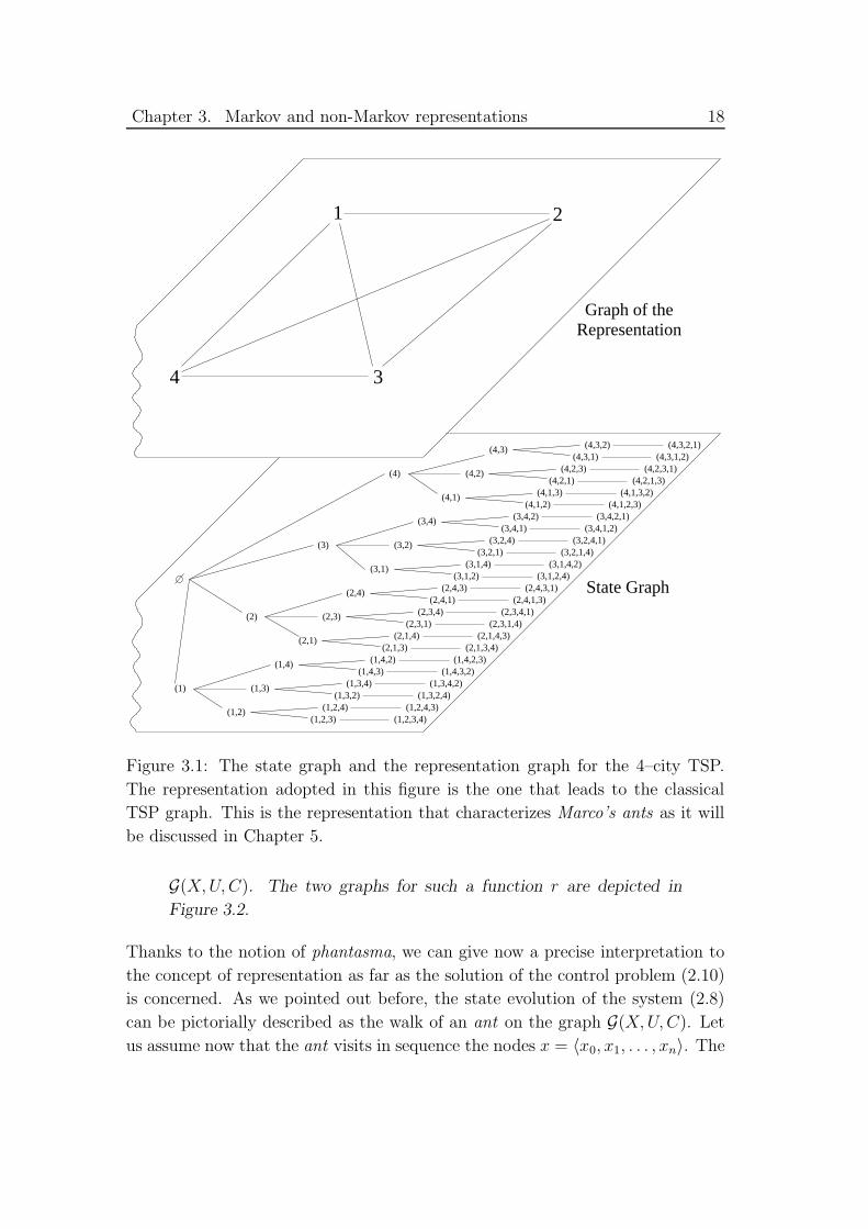
Example: In the case of the 4–city TSP considered in our examples,

the function r might be for instance defined as a function that maps

the set X \ {x0} to Zr = Y . In particular, and this is the case that

will be of interest in the following, we will define r such that a state

xτ whose last component is uτ−1 = yi is mapped on the phantasma

zt = yi. Figure 3.1 shows the graph Gr(Zr, Ur, T ) of the representation

generated by such a function r, together with the original state graph

G(X, U, C).

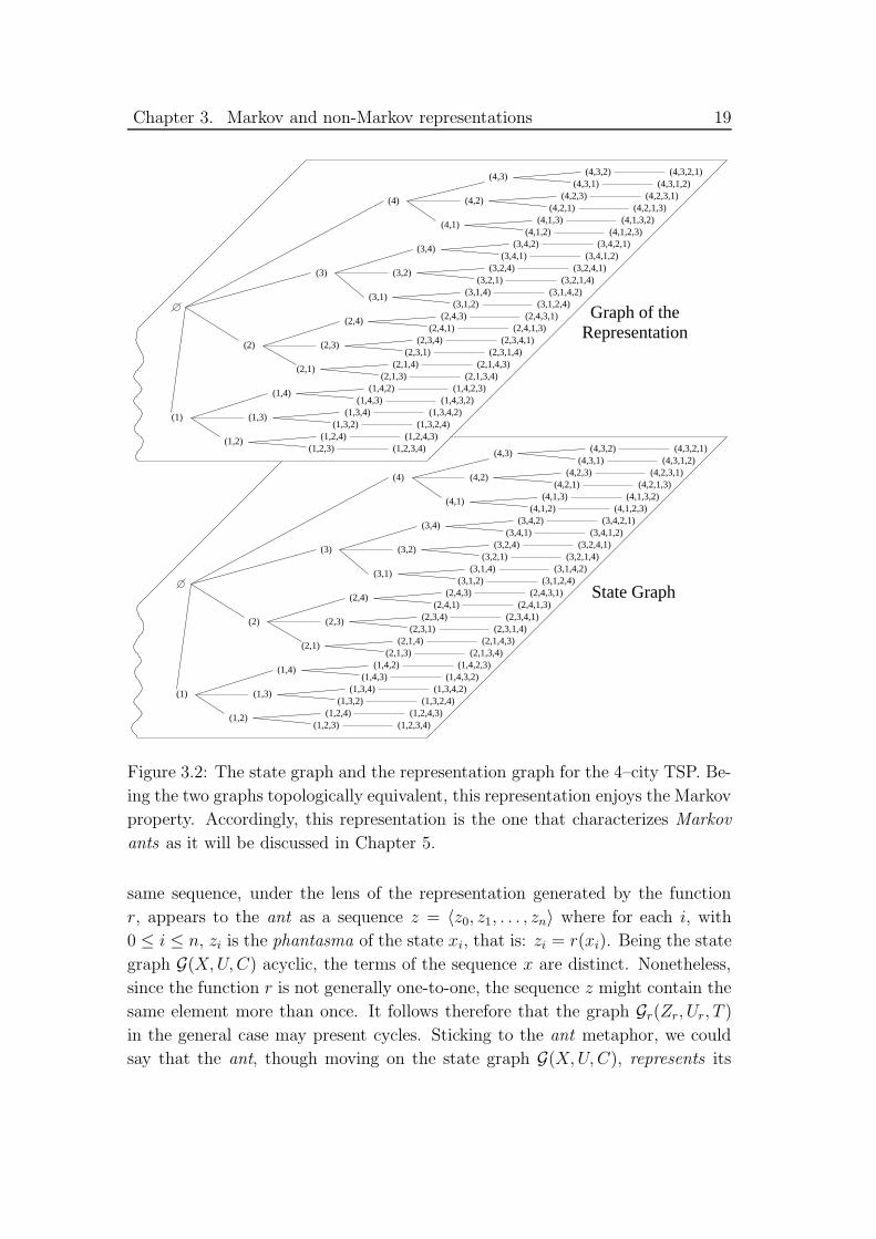
Another possible definition of the function r that will be of inter-

est in the following is the one that considers as generating function

the identity function. In this case, the graph of the representation

Gr(Zr, Ur, T ) has the same topological structure as the state graph

3In some cases, for convenience, the generating function of the representation can be defined

as r : X \{x0} → Zr. For ease of description and for avoiding to the reader details of secondary

importance, this is the case we will consider in our examples. Despite this minor difference,

our analysis remains essentially unchanged.4Aristotle (384–322 BC) De Anima: “The soul never thinks without a mental image.”

Aristotle uses here the term phantasma to mean what can be nowadays translated as mental

image.5Thomas Aquinas (1225–1274) Summa Theologiae.

Chapter 3. Markov and non-Markov representations 18

Graph of theRepresentation

1

4

2

3

State Graph

(1,2,3)(1,2,4)

(2,1,3)(2,1,4)

(2,3,1)(2,3,4)

(2,4,1)(2,4,3)

(3,1,2)(3,1,4)

(3,2,4)(3,4,1)

(4,2,3)(4,3,1)

(4,3,2)

(1,2,3,4)(1,2,4,3)

(1,3,2,4)(1,3,4,2)

(1,4,3,2)(1,4,2,3)

(2,1,3,4)(2,1,4,3)

(2,3,1,4)(2,3,4,1)

(2,4,1,3)(2,4,3,1)

(3,1,2,4)(3,1,4,2)

(3,2,1,4)(3,2,4,1)

(3,4,1,2)(3,4,2,1)

(4,1,2,3)(4,1,3,2)

(4,2,1,3)(4,2,3,1)

(4,3,1,2)(4,3,2,1)

(1,4)

(2,1)

(2,3)

(2,4)

(3,1)

(3,2)

(3,4)

(4,1)

(4,2)

(4,3)

(1,2)

(1,3)(1)

(2)

(3)

(4)

(1,3,2)(1,3,4)

(1,4,3)(1,4,2)

(3,2,1)

(3,4,2)(4,1,2)

(4,1,3)(4,2,1)

Figure 3.1: The state graph and the representation graph for the 4–city TSP.

The representation adopted in this figure is the one that leads to the classical

TSP graph. This is the representation that characterizes Marco’s ants as it will

be discussed in Chapter 5.

G(X, U, C). The two graphs for such a function r are depicted in

Figure 3.2.

Thanks to the notion of phantasma, we can give now a precise interpretation to

the concept of representation as far as the solution of the control problem (2.10)

is concerned. As we pointed out before, the state evolution of the system (2.8)

can be pictorially described as the walk of an ant on the graph G(X, U, C). Let

us assume now that the ant visits in sequence the nodes x = 〈x0, x1, . . . , xn〉. The

Chapter 3. Markov and non-Markov representations 19

State Graph

Graph of theRepresentation

(1,2,3)(1,2,4)

(2,1,3)(2,1,4)

(2,3,1)(2,3,4)

(2,4,1)(2,4,3)

(3,1,2)(3,1,4)

(3,2,4)(3,4,1)

(4,2,3)(4,3,1)

(4,3,2)

(1,2,3,4)(1,2,4,3)

(1,3,2,4)(1,3,4,2)

(1,4,3,2)(1,4,2,3)

(2,1,3,4)(2,1,4,3)

(2,3,1,4)(2,3,4,1)

(2,4,1,3)(2,4,3,1)

(3,1,2,4)(3,1,4,2)

(3,2,1,4)(3,2,4,1)

(3,4,1,2)(3,4,2,1)

(4,1,2,3)(4,1,3,2)

(4,2,1,3)(4,2,3,1)

(4,3,1,2)(4,3,2,1)

(1,4)

(2,1)

(2,3)

(2,4)

(3,1)

(3,2)

(3,4)

(4,1)

(4,2)

(4,3)

(1,2)

(1,3)(1)

(2)

(3)

(4)

(1,3,2)(1,3,4)

(1,4,3)(1,4,2)

(3,2,1)

(3,4,2)(4,1,2)

(4,1,3)(4,2,1)

(1,2,3)(1,2,4)

(2,1,3)(2,1,4)

(2,3,1)(2,3,4)

(2,4,1)(2,4,3)

(3,1,2)(3,1,4)

(3,2,4)(3,4,1)

(4,2,3)(4,3,1)

(4,3,2)

(1,2,3,4)(1,2,4,3)

(1,3,2,4)(1,3,4,2)

(1,4,3,2)(1,4,2,3)

(2,1,3,4)(2,1,4,3)

(2,3,1,4)(2,3,4,1)

(2,4,1,3)(2,4,3,1)

(3,1,2,4)(3,1,4,2)

(3,2,1,4)(3,2,4,1)

(3,4,1,2)(3,4,2,1)

(4,1,2,3)(4,1,3,2)

(4,2,1,3)(4,2,3,1)

(4,3,1,2)(4,3,2,1)

(1,4)

(2,1)

(2,3)

(2,4)

(3,1)

(3,2)

(3,4)

(4,1)

(4,2)

(4,3)

(1,2)

(1,3)(1)

(2)

(3)

(4)

(1,3,2)(1,3,4)

(1,4,3)(1,4,2)

(3,2,1)

(3,4,2)(4,1,2)

(4,1,3)(4,2,1)

Figure 3.2: The state graph and the representation graph for the 4–city TSP. Be-

ing the two graphs topologically equivalent, this representation enjoys the Markov

property. Accordingly, this representation is the one that characterizes Markov

ants as it will be discussed in Chapter 5.

same sequence, under the lens of the representation generated by the function

r, appears to the ant as a sequence z = 〈z0, z1, . . . , zn〉 where for each i, with

0 ≤ i ≤ n, zi is the phantasma of the state xi, that is: zi = r(xi). Being the state

graph G(X, U, C) acyclic, the terms of the sequence x are distinct. Nonetheless,

since the function r is not generally one-to-one, the sequence z might contain the

same element more than once. It follows therefore that the graph Gr(Zr, Ur, T )

in the general case may present cycles. Sticking to the ant metaphor, we could

say that the ant, though moving on the state graph G(X, U, C), represents its

Chapter 3. Markov and non-Markov representations 20

Graph of theRepresentation

1

4

2

3

State Graph

(1,2,3)(1,2,4)

(2,1,3)(2,1,4)

(2,3,1)(2,3,4)

(2,4,1)(2,4,3)

(3,1,2)(3,1,4)

(3,2,4)(3,4,1)

(4,2,3)(4,3,1)

(4,3,2)

(1,2,3,4)(1,2,4,3)

(1,3,2,4)(1,3,4,2)

(1,4,3,2)(1,4,2,3)

(2,1,3,4)(2,1,4,3)

(2,3,1,4)(2,3,4,1)

(2,4,1,3)(2,4,3,1)

(3,1,2,4)(3,1,4,2)

(3,2,1,4)(3,2,4,1)

(3,4,1,2)(3,4,2,1)

(4,1,2,3)(4,1,3,2)

(4,2,1,3)(4,2,3,1)

(4,3,1,2)(4,3,2,1)

(1,4)

(2,1)

(2,3)

(2,4)

(3,1)

(3,2)

(3,4)

(4,1)

(4,2)

(4,3)

(1,2)

(1,3)(1)

(2)

(3)

(4)

(1,3,2)(1,3,4)

(1,4,3)(1,4,2)

(3,2,1)

(3,4,2)(4,1,2)

(4,1,3)(4,2,1)

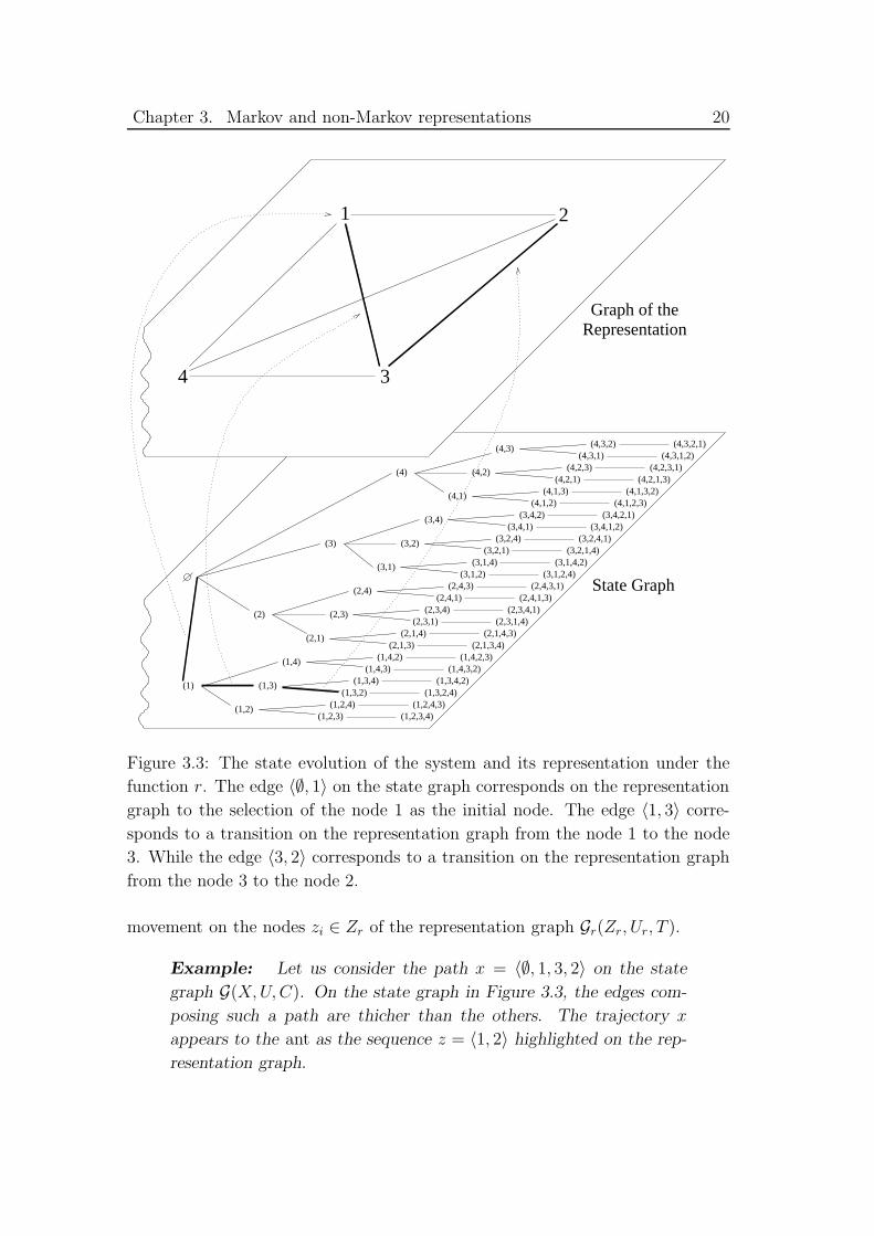
Figure 3.3: The state evolution of the system and its representation under the

function r. The edge 〈∅, 1〉 on the state graph corresponds on the representation

graph to the selection of the node 1 as the initial node. The edge 〈1, 3〉 corre-

sponds to a transition on the representation graph from the node 1 to the node

3. While the edge 〈3, 2〉 corresponds to a transition on the representation graph

from the node 3 to the node 2.

movement on the nodes zi ∈ Zr of the representation graph Gr(Zr, Ur, T ).

Example: Let us consider the path x = 〈∅, 1, 3, 2〉 on the state

graph G(X, U, C). On the state graph in Figure 3.3, the edges com-

posing such a path are thicher than the others. The trajectory x

appears to the ant as the sequence z = 〈1, 2〉 highlighted on the rep-

resentation graph.

Chapter 3. Markov and non-Markov representations 21

In the literature on control theory and system identification, the above described

process which carries the state into what we call here phantasma, is related to

the concept of state-space reduction.6 Another notion that arises in control the-

ory and system identification, and that is significantly related to the concept of

phantasma, is the notion of (incomplete) state reconstruction. Both concepts [16]

are related to the necessity of gathering information on the state of the system

in order to perform a control action, nonetheless, it is important to keep these

two concepts separated.

The problem of state reconstruction arises when it is not possible to have

access immediately to the state of the system, usually a physical entity, but re-

lated quantities are readable and have been read and stored in some appropriate

preceding time window. The case discussed in this thesis is significantly different.

The system (2.8) is a mathematical entity that bears no direct relation with any

physical device: It is simply an abstract description of the incremental construc-

tion of a feasible solution of the optimization problem (2.3). The state of such

a system is therefore immediately readable and, in principle, usable in order to

select a feasible control action. Still, it is easy to verify that in many cases of

great practical importance, think for example of NP-hard problems, the number

of nodes of the state graph grows more than polynomially with the number of

problem components, making infeasible any solution method that relies directly

on a state description. Therefore, it might become desirable, or even necessary,

the use of some quantity related to the state but more easily manageable. This

quantity, that can be obtained via a heuristic method that allows to move from

the state graph G of the system to a smaller and more manageable representation

graph Gr, is the phantasma discussed in this thesis.

This change of representation is by no means free from complications. While

in the graph G every (partial) path is a (partial) feasible solution and vice versa,

in the graph Gr this property does not hold anymore: to every (partial) solution

a path on the graph Gr can be associated, but the opposite in not true. As far as

the construction of feasible solutions is concerned, the graph G is not therefore

superseded by Gr.

As anticipated before, the graph Gr and the information stored on it are used

to take decisions while a solution is being built. Because of the loss of topological

information induced by the transformation from G to Gr, in the general case only

6Nevertheless, the result of a state-space reduction does not have a standard name in system

and control theory. Moreover, the terms used in the literature always bring a direct reference to

the concept of state: i.e. reduced state. It is just in order to underline the important qualitative

difference between the properties of the state and those of the result of a state-space reduction,

that we introduce here the term phantasma to denote the latter.

Chapter 3. Markov and non-Markov representations 22

sub-optimal solutions will be obtained.

In this sense, while the reconstruction of the state is related to a process in

which one indeed tries to construct a quantity related to the state starting from

simpler pieces of information that are directly readable, a phantasma is related to

a reduction process that goes in the opposite direction: The state is itself directly

available but it is de-constructed in order to obtain a representation that be more

manageable.

In the same spirit of the definition of the set Zr, also the set of the edges Ur

can be defined in terms of the generating function r. The set Ur ⊂ Zr ×Zr is the

set of the edges 〈zi, zj〉 for which it exists an edge of the state graph 〈xi, xj〉 ∈ U ,

such that xi and xj are the preimages under r of zi and zj, respectively. Formally:

Ur ={

〈zi, zj〉∣

∣ ∃〈xi, xj〉 ∈ U : zi = r(xi), zj = r(xj)}

.

The major difficulty that arises when the system is described through a generic

representation r, is that the subset Ur(t) ⊂ Ur of the admissible control actions at

time t, usually cannot be described in terms of the phantasma zt alone, but needs

for its definition the knowledge of the underlying state xt. More in detail, when

the agent observes the phantasma zt, a transition 〈zt, zt+1〉 towards the phantasma

zt+1 is admissible only if it exists the edge 〈xt, xt+1〉 ∈ U(xt), where xt, among all

the preimages r−1({zt}) of the phantasma zt, is the actual current state which

gave rise to zt itself, and where r(xt+1) = zt+1.

Such a fact shows clearly that for the generic generating function r, the phan-

tasma does not enjoy the first property of the definition of state given above and

therefore the corresponding representation is non-Markov. Anyway, it is always

possible to obtain at least one representation that enjoys the Markov property.

In particular, in order to obtain a Markov representation it is sufficient that

the function r be one-to-one, and the most trivial Markov representation can be

obtained by posing r ≡ I, where I is the identity function.

In the general case, the parallel of the function C of G for the graph Gr cannot

be defined in a straightforward manner. Moreover, it results more useful to define

the weights of the edges of the graph Gr(Zr, Ur, T ) so that they describe the

quantity that in ant colony optimization is called pheromone trail. The function

T : Ur → R will be used in the process of selecting an action by an ant when

perceiving a given phantasma, and will be iteratively modified in order to improve

the quality of the solutions generated. A thorough definition and analysis of the

function T will be given in Chapter 4.

It is anyway worth discussing here the difficulties that arise when trying to

define, on the basis of C, a function that maps an edge 〈zt, zt+1〉 of Gr to a

Chapter 3. Markov and non-Markov representations 23

cost. Let the agent that observes the system through the representation r see,

for instance, a transition from the phantasma zt to the phantasma zt+1, without

being aware of the details of the underlying state transition from xt to xt+1. The

only thing that the agent is able to induce about the state description from his

observations, is that some transition has occurred between a state belonging to

the set of preimages r−1({zt}) of the phantasma zt, to one belonging to the set

of preimages r−1({zt+1}) of the phantasma zt+1. Together with such a transition

〈zt, zt+1〉, the agent experiences the cost ct+1 associated to the underlying tran-

sition 〈xt, xt+1〉 by the function C. Such cost is indeed a deterministic function

determined univocally by 〈xt, xt+1〉. Nonetheless, for the agent that observes the

system through a generic representation r, such a cost can at best be expressed as

a stochastic quantity only partially determined by 〈zt, zt+1〉 ∈ Ur. More precisely,

on the sole basis of the knowledge that the current phantasma is zt, the agent

might expect to observe a cost belonging to the following set:

{

c∣

∣ c = C(〈xi, xj〉) with xi ∈ r−1(

{zt})

, xj ∈ r−1(

{zt+1})

}

. (3.3)

In the following, we consider cases in which although a Markov representation of

the underlying system can be easily obtained, it is convenient, for computational

reasons, to consider a representation of non-Markov type. In particular, the

concepts of Markov and non-Markov representations are the key elements for the

definition of the class of algorithms that we call ant programming and that will

be introduced in the next chapter. Among the possible different instances of

this class of algorithms, the most significative are those that adopt a somehow

extreme attitude towards Markovianity. On the one hand, Markov ants give, of

the underlying problem at hand, a faithful representation that enables to find the

optimal solution, but that for larger problems leads to intractability. On the other

hand, Marco’s ants, by adopting a non-Markov representation, are not guaranteed

to find the optimal solution but handle a more compact representation graph and

therefore in practice revealed to be much more suitable for larger problems.

Chapter 4

Ant programming

In this chapter we introduce a new class of algorithms which deal with the op-

timization problems (2.3) under the form described by (2.10). The class of al-

gorithms we introduce here is inspired by ant colony optimization, and from the

latter it inherits the essential features, the terminology and the underlying phi-

losophy.

The aim of this chapter is mostly speculative: we do not describe here a spe-

cific algorithm, but rather a class in the sense that we define a general resolution

strategy and an algorithmic structure where some components are functionally

specified but left uninstantiated.

In the following, with ant programming we will refer to this class of algorithms

together with the collection of problems (2.3) or equivalently (2.10).

Ant programming is introduced here mainly as a mean to gain insight into the

general principles underlying the use of a Monte Carlo approach for the solution

of the class of problems (2.3). Such an insight will throw a new light on ant

colony optimization itself.

4.1 The three phases of ant programming

Two are the essential features of ant programming. The first is the incremental

Monte Carlo generation of complete paths over the state graph G, on the basis of

information contained in the representation graph Gr. The second is the use of

the cost of the generated solutions to bias subsequent generations of paths. These

two features are described in terms of the three phases which, properly iterated,

constitute ant programming : At each iteration, a cohort of ants is considered.

Each ant in the cohort undergoes a forward phase that determines the generation

of a path, and a backward phase that states how the costs experienced along such

24

Chapter 4. Ant programming 25

a path should influence the generation of future paths. Finally, each iteration is

concluded by a merge phase that combines the contribution of all the ants of the

cohort.

The three phases forward, backward, and merge are in turn characterized

by the three operators πε, ν, and σ respectively. The following sections give a

detailed analysis of these elements of ant programming.

4.1.1 Monte Carlo generation of paths: The “forward”

phase

Using the terminology inherited from ant colony optimization and in the light of

the formalization given in Chapter 3, ant programming metaphorically describes

each Monte Carlo run as the walk of an ant over the graph G(X, U, C), where

at each node a random experiment determines the following node. In the ant

metaphor, the random experiment is depicted as a decision taken by the ant on

the basis of a probabilistic policy parameterized in terms of information contained

in the graph Gr(Zr, Ur, T ).

Let us give a detailed description of this decision process that will be hereafter

denoted as the forward phase. Let us suppose that after t decision steps the

partial solution built so far is (u0, . . . , ut−1). The state of the solution generation

process is therefore xt = (u0, . . . , ut−1). In the ant metaphor, this fact is visualized

as an ant being in the node xt of the graph G(X, U, C). The ant perceives the

state xt in terms of the phantasma zt = r(xt) of the graph Gr(Zr, Ur, T ). In

the general case, it is not possible to express the set Ur(t) of admissible actions

available to the ant when in zt only in terms of zt itself, and of the information

contained in Gr. Indeed, it is necessary the knowledge of the actual state xt, and

of the set U(xt) of the edges departing from node xt in the graph G. The set Ur(t)

of the admissible actions at time t is indeed:

Ur(t) = Ur(zt|xt) ={

〈zt, zt+1〉 ∈ Ur

∣

∣ zt+1 ∈ r(

U(xt))

, zt = r(xt)}

.

The decision of the ant consists in the selection of one element from the set

Ur(zt|xt) of the available transitions, as described at the level of the graph Gr.

Once an element, say 〈zt, zt+1〉, is selected, the partial solution is transformed

according to Eq. 2.4 and Eq. 2.9:

xt+1 = [xt, ut] = (u0, . . . , ut−1, ut),

where xt+1 ∈ r−1({zt+1}) is one of the preimages of the phantasma zt+1. If more

than one preimage exist, one among them is arbitrarily selected. In terms of

Chapter 4. Ant programming 26

the metaphor, this state transition is described as a movement of the ant to

the node xt+1 of G which in turn is perceived by the ant as a movement to the

phantasma zt+1 = r(xt) on Gr.

The decision among the elements of Ur(zt|xt) is taken according to the first

operator of ant programming : the stochastic policy πε. Given the current phan-

tasma and the set of admissible actions Ur(zt|xt), the policy selects an element of

Ur(zt|xt) as the outcome of a random experiment whose parameters are defined

by the weights T (〈zt, zt+1〉) of the edges Ur(zt|xt) on the graph Gr(Zr, Ur, T ).

Accordingly we will adopt the following notation to denote the stochastic policy:

πε

(

zt, Ur(zt|xt); T |Ur(zt|xt)

)

. (4.1)

With the notation T |Ur(zt|xt) we want to suggest that, when in zt, the the full

knowledge of the function T is not strictly needed in order to select an element of

the set Ur(zt|xt). Indeed it is sufficient to know the restriction of T to the subset

Ur(zt|xt) of the domain Ur of T .1

In relation to the definition of the policy πε, it is worth noticing here how the

decision process uses the information contained in the two graphs G and Gr: The

decision is taken on the basis of information pertaining to the graph Gr, restricted

by the knowledge of the actual state xt which in turn is a piece of information

pertaining to the graph G.

For future reference, it is important to notice that T , that is, the weights of

the graph Gr, are to be intended as parameters of the policy πε: Changing the

weights of Gr amounts therefore to changing the policy itself. Further, in the

following the subscript ε will indicate, in a sense that will depend on the actual

implementation of πε, the degree of stochasticity of the policy, such that ε = 0 will

mean a deterministic policy. For the moment, the reader can see the subscript

as a mere reminder of the possibly stochastic nature of the policy πε.

Given the abstract definition (4.1) of the policy πε, the forward phase can

be defined as the sequence of steps that take one ant from the initial state x0,

to a solution, say s = xτ , of the original combinatorial problem (2.3). Each of

such steps is composed by the two operations of first selecting a transition on the

graph Gr, and then actually moving on the graph G from the current node xt to

1This fact is the expression of one of the feature of ant programming, namely the locality of

the information needed by the ant in order to take each elementary decision. Such a feature

plays and important role in the implementation, allowing a distribution of the information on

the graph of the representation Gr.

Chapter 4. Ant programming 27

the neighboring node xt+1. Formally, the single forward step is described as:

〈zt, z′t+1〉 = πε

(

zt, Ur(zt|xt); T |Ur(zt|xt)

)

;

xt+1 = F(

xt, 〈zt, z′t+1〉

)

;

zt+1 = r(xt+1),

(4.2)

where the operator πε is the stochastic policy that indicates the transition to be

executed as seen on the graph Gr, and where with the operator F we denote the

operation of selecting one preimage xt+1 of z′t+1 and moving to it on the graph G

from the current state xt. Such a movement on G will be indeed perceived by the

ant as a movement to the phantasma zt+1 = r(xt+1) = z′t+1, as requested by the

policy πε.

4.1.2 Biasing the generation of paths: The “backward”

and the “merge” phases

The ultimate goal of ant programming is to find a policy πε, not necessarily

stochastic, such that a sequence of decisions taken according to πε leads an ant

to define the solution s which minimizes the cost function J of the original opti-

mization problem (2.3).

Since the generic policy (4.1) is described parametrically in terms of the func-

tion T , that is, in terms of the weights associated to the edges of the graph Gr, a

search in the space of the policies amounts to a search in the space of the possible

weights of the graph Gr itself.

From a conceptual point of view, the function T is to be related to Hamilton’s

principal function of the calculus of variations, and to the cost-to-go and value

function of dynamic programming and reinforcement learning. More precisely,

the function T can be closely related to the function that in the reinforcement

learning literature is known as “state-action value function,” and that is custom-

arily denoted by the letter Q.2

2For the benefit of the reader who is not deeply acquainted with reinforcement learning

theory, we note that a reference to the Q function does not necessarily imply a reference to

Q-learning. The latter is a specific algorithm for learning a Q function. The Q function itself

is the more general concept of a function that associates a number to a state-action pair, the

number being the total future cost that would be incurred if, from the given state, one selects

the given action and then behaves optimally thereafter.

A further terminological remark involves the reason why the word “state” is italicized in the

previous sentence. As argued in Section 3.2, a state enjoys the Markov property by definition

and therefore a “non-Markov state” is, in this sense, a contradiction in terms. Nevertheless,

in the reinforcement learning literature it is customary to refer to the concept of “state” and

Chapter 4. Ant programming 28

A complete analysis of how to express the Q function for the problem at hand

in terms of the function T is, at this stage of our argumentation, not possible yet.

For the time being, it will be sufficient to notice that T (〈zt, zt+1〉) determines, as

to Eq. 4.1, the probability of selecting the action “go to phantasma zt+1” when

the current phantasma is zt. It therefore associates to the phantasma-action pair,

a number which represents the desirability of performing such an action in the

given phantasma. In this respect, and taking into account the remark of Note 2,

it is clear the similarity with the role of the function Q in reinforcement learning.

Moreover, as it will be made clear presently, the value of T (〈zt, zt+1〉) is generally

given as a statistic of the observed cost of paths containing the transition 〈zt, zt+1〉.

It therefore brings information on the quality of the solution that can be obtained

by “going to zt+1” when in zt. Also in this respect, it can be stated a parallel

with the function Q which indeed informs on the long-term cost of a given action,

provided that future actions are selected optimally.

In ant programming, as generally in reinforcement learning, the search in the

space of the policies is performed through some form of generalized policy itera-

tion [22]. Starting from some arbitrary initial policy, ant programming iteratively

generates a number of paths in order to evaluate the current policy and then im-

proves it on the basis of the result of the evaluation.

At each iteration, therefore, a cohort of ants is considered, each generating a

solution through a forward phase as described in the previous section. Once the

solution is completed, each ant traces back its path proposing a new value of the

function T on the basis of the costs experienced in the forward movement—and

possibly on the basis of the current value of T . This phase is denoted in the

terminology of ant programming as the backward phase of the given ant. The

actual new value of T is obtained by some combination of the values proposed

by the ants of the cohort. This phase is denoted as the merge phase.

Let us now see in detail the backward phase for a given single ant. Let us

consider a complete path x = 〈x0, x1, . . . , xτ 〉 over the graph G. Let s = xτ be

the solution associated to the path x, and c = 〈c1, . . . , cτ 〉 be the sequence of

to adopt the above mentioned definition of Q irrespectively, both when the Markov property

holds, and when it does not.

In general, we regard this abuse of terminology as bad practice. Though usually this does

not cause major harms, it introduces unnecessary inconsistencies between the literature in

reinforcement learning on the one side, and “more classical” fields as control theory or system

theory on the other. Because in this work we refer both to the level of the state description and

to the level of the representation, it is particularly important to be strict with the distinction

between the concept of state and the concept of phantasma. According to the terminology

introduced in Section 3.3, the function Q is to be defined as Q : Z ×U → R. It therefore maps

a phantasma-action pair into a number.

Chapter 4. Ant programming 29

costs experienced along the path. Further, let z = 〈z0, z1, . . . , zτ 〉 be the path x

as perceived by the ant under the representation r. That is, zt = r(xt) with

t = 0, . . . , τ .

The key element of the backward phase is the operator ν that uses the observed

costs associated to the solution s in order to propose a new function T ′. Similarly

to the forward phase, the backward phase is composed by a sequence of steps,

each formally described by the pair of operations:

zt = B(zt+1, z),

T ′(〈zt, zt+1〉) = ν(c, T ),(4.3)

where with the operator B we indicate a single step backward on the graph Gr,

along the forward trajectory z. The operator ν proposes a new value for the

weight associated to each visited edge 〈zt, zt+1〉, on the basis of the sequence of

costs experimented during the forward phase, and of the current values of the

function T .

It is intuitive that each single ant proposes values of T ′ for those transitions

〈zt, zt+1〉 that it has experienced along the path z, and leaves undetermined those

related to unseen transitions. Hence, in our pictorial description of ant program-

ming, this phase is pictured through an ant that “traces back” its forward path

and leaves on such a path some information.

From a logical point of view, the different strategies for propagating the infor-

mation gathered along a path are to be related to the different update strategies

in reinforcement learning. In particular, for an ant to propose values of T ′ only

for the visited transitions and on the basis of the cost of the associated solution,

is equivalent to what in reinforcement learning is called Monte Carlo update [22].

On the other hand, it is equivalent to a Q-learning update [23] to propose a value

of T ′ for a visited transition on the basis of the experienced cost for the transi-

tion itself and of the minimum of the current values that T assumes on the edges

departing from the node to which the considered transition leads.

The details of the definition of the backward phase, and in particular of the

operator ν are not given as part of the description of ant programming and are

left uninstantiated.

In the same spirit, we leave here undefined in its details also the merge phase

in which it is performed a combination of the different functions T ′ proposed by

the individual ants of the same cohort. At this level of our description it will be

sufficient to note that, for every transition 〈zt, zt+1〉 ∈ Ur, the actual new value

of T (〈zt, zt+1〉) will be some linear or nonlinear function of the current value of

T (〈zt, zt+1〉), and of the different T ′j(〈zt, zt+1〉), where j is the index ranging over

Chapter 4. Ant programming 30

the ants of the cohort. The merge phase will be therefore characterized by the

operator σ:

T (〈zt, zt+1〉) = σ(

T (〈zt, zt+1〉), T′1(〈zt, zt+1〉), T

′2(〈zt, zt+1〉), . . .

)

. (4.4)

Different possible instances of the operators ν and σ will be discussed in a future

work.

4.2 The algorithm and the metaphor

The abstract definition of ant programming has been given in the previous sections

in terms of the operators πε, ν, and σ. In order to define an instance of the ant

programming class, such operators need to be instantiated and defined in their

details. Together with the operators πε, ν, and σ, the other key element in the

definition of an instance of the class, is the generating function r that defines the

relation between the state graph G and the representation Gr. We will therefore

denote an instance of ant programming with the 4-tuple

〈r, πε, ν, σ〉. (4.5)

Indeed, other elements are to be instantiated as, for instance, the way to select

one preimage of a given phantasma in Eq. 4.2, or the number N of ants composing

a cohort and the way of initializing the function T . Anyway, such elements are

either less relevant, or are to be defined as a more or less direct consequence

of the definition of the 4-tuple (4.5). For the sake of clarity and readability of

the notation, we will therefore adopt Expression 4.5 to denote an instance of

ant programming. In future developments, if it will be necessary to make the

distinction between two instances that differ only for elements other than those

considered in the 4-tuple, Eq. 4.5 will be extended to include the elements that

are needed in order to refer univocally to each of the instances under analysis.

In particular, the 4-tuple (4.5) gives an operative definition of the function T ,

which is the function that the algorithm iteratively modifies and refines with

the aim of converging to an optimal policy. As seen in the previous sections,

the generating function r, together with the graph G, gives the topology of the

graph Gr and determines therefore the domain of the function T . The operator πε

defines how the values of T are used in the decision process, while the operators ν

and σ define how the function T is to be modified on the basis of the quality of

the solutions obtained.

Considered the key role of the function T in ant programming, we now provide

this function with an interpretation in terms of the ant metaphor. At the same

time, this will complete the pictorial description of the algorithm.

Chapter 4. Ant programming 31

As anticipated in Section 3.3, the value T (〈zt, zt+1〉) associated to the edge

〈zt, zt+1〉 is called, in the ant metaphor, the value of the pheromone trail on

the edge 〈zt, zt+1〉 itself. A single Monte Carlo run is described by an ant that

walks on the graph G, starting from the node x0, and incrementally builds the

solution s of cost J(s). Each visited state xt, is indeed perceived by the ant as

the phantasma zt = r(xt). At each time step, the following node xt+1 is selected

by the procedure described by the forward step (4.2). Such procedure involves a

decision taken by the ant according to the policy πε and therefore according to

the value of the pheromone trail on the edges of Gr, departing from the current

phantasma.

Once the solution s is completed, the ant traces back the path that led to the

solution itself, and deposits its pheromone. Out of the metaphor, the values of

the function T are changed for those edges 〈zt, zt+1〉 that describe on the graph Gr

the path leading to the solution s.

The role of the pheromone trails T is to make available the information gath-

ered on a particular path by one ant belonging to one given cohort, to other ants

of a future cohort ; it is therefore a form of inter-cohort communication mediated

by the graph Gr. For real insects, the notion of stigmergy [17] has been introduced

to denote a form of “stimulation [. . . ] by the very performance [. . . ] achieved.”

More in general, the term has been used to describe any indirect communica-

tion mediated by modification of the environment that can be observed in social

insects [6, 9]. Accordingly, in the ant metaphor it is customary to refer to the

interaction between ants with the term stigmergy [11].

As a way to give a summary of the concepts discussed in this section, we

propose in Table 4.1 a pseudo-code description of ant programming.

At this point, having defined the 4-tuple (4.5), we have completed the def-

inition and the analysis of the essential elements that are necessary to handle

the complexity of the combinatorial problem (2.3), in the spirit of the solution

strategy originally suggested by ant colony optimization. In this sense, ant pro-

gramming, beside defining a general strategy for solving the combinatorial prob-

lem (2.3), provides also a formal tool for gaining some further insight in the deep

motivations of ant colony optimization.

In particular, ant programming defines the notion of a generic generating func-

tion of the representation, keeping therefore separated the problem at hand, from

the problem representation that is assumed by the solution strategy. As a conse-

quence, it becomes clear that the key element for understanding the properties of

ant colony optimization is the the relation existing between state and phantasma,

and between the graphs G and Gr.

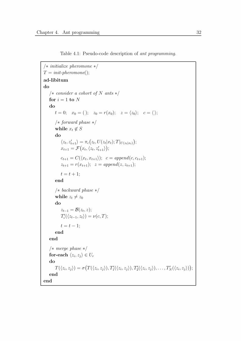
Chapter 4. Ant programming 32

Table 4.1: Pseudo-code description of ant programming.

/∗ initialize pheromone ∗/

T = init-pheromone();

ad-libitum

do

/∗ consider a cohort of N ants ∗/

for i = 1 to N

do

t = 0; x0 = ( ); z0 = r(x0); z = 〈z0〉; c = 〈 〉;

/∗ forward phase ∗/

while xt 6∈ S

do

〈zt, z′t+1〉 = πε

(

zt, U(zt|xt); T |U(zt|xt)

)

;

xt+1 = F(

xt, 〈zt, z′t+1〉

)

;

ct+1 = C(〈xt, xt+1〉); c = append(c, ct+1);

zt+1 = r(xt+1); z = append(z, zt+1);

t = t + 1;

end

/∗ backward phase ∗/

while zt 6= z0

do

zt−1 = B(zt, z);

T ′i (〈zt−1, zt〉) = ν(c, T );

t = t − 1;

end

end

/∗ merge phase ∗/

for-each 〈zi, zj〉 ∈ Ur

do

T (〈zi, zj〉) = σ(

T (〈zi, zj〉), T′1(〈zi, zj〉), T

′2(〈zi, zj〉), . . . , T

′N(〈zi, zj〉)

)

;

end

end

Chapter 4. Ant programming 33

Even if the knowledge of the state is still necessary to the policy πε in order

to check on-line the feasibility of the solution being built, the optimization of the

decision process and the search for the optimal policy act on the function T and

therefore refer only to the graph of the representation Gr. If the generating func-

tion of the representation is not selected trivially as r ≡ I, the number of edges

of the graph Gr might be dramatically smaller than the one of G. In particular,

for an appropriate choice of the function r, the number of the edges of Gr might

grow polynomially with the number |Y | of component of the original optimization

problem, even if the number of edges of the graph G grows exponentially.

Actually, the above described process is the one carried out by ant colony

optimization. There, the generating function r, though not explicitly mentioned,

is implicitly defined in a way that reduces dramatically the complexity of the

graph on which the ants move. A preliminary analysis of the relation between

ant colony optimization and the general ant programming method, is sketched in

Chapter 5 with the definition of the specific instance of ant programming that we

call Marco’s ants.

Chapter 5

Conclusions and future work

This thesis addresses the definition of formal tools for the analysis of ant colony

optimization, a class of algorithms for solving heuristically a discrete optimization

problem with a finite number of solutions. To this aim we introduce the more

general and abstract framework of ant programming.

Inspired by the foraging behavior of real ants, ant colony optimization pro-

poses a heuristic solution to the problem at hand, through a process that involves

iterated generations of paths on an appropriate graph. The generation of each

path is described in terms of a metaphor by the walk of an ant, and represents

the incremental construction of a feasible solution of the original combinatorial

problem.

The incremental generation of solutions considered in ant colony optimization

suggested a representation of the original combinatorial optimization problem in

terms of a finite-horizon multi-stage decision process that can be thoroughly seen

as a discrete-time optimal control problem. In turn, such an optimal control

problem can be naturally mapped on the problem of finding paths of minimum

cost on a graph whose nodes represent states of the controlled system. In other

words, the incremental generation of a solution of the original combinatorial

problem can be seen as the generation of a path on a graph.

The thesis proposes a critical analysis of the concept of state of the process

which incrementally constructs a solution of a combinatorial problem. Further,

the thesis draws a clear picture of the relation between concepts pertaining to

this context and their natural counterparts in control theory. As a result of this

analysis, a clear understanding emerges about the notions of representation and of

Markov property in relation to the class of combinatorial optimization problems.

This understanding will be of particular importance for future developments of

ant programming.

34

Chapter 5. Conclusions and future work 35

In particular, working on a Markov representation of an NP-hard problem

is computationally infeasible. Therefore, the need emerges clearly for a compu-

tational method that generate a manageable representation, though this can be

obtained only at the expense of the Markov property.

In order to give a well defined meaning to the previous sentence, the thesis

introduces the notion of phantasma as the piece of information, somehow related

to the state, on the basis of which all the decisions are taken in the incremental

construction of a solution.

In this thesis, ant programming is introduced as an abstract class of algorithms

inspired by ant colony optimization, and inheriting from it the essential features,

the terminology, and the underlying philosophy.

Ant programming is an abstract class of algorithms in the sense that some

of its elements are only functionally defined, and are left uninstantiated in their

details. Indeed, ant programming has been introduced as a mean for gaining

insight into the general principles underlying the use of a Monte Carlo approach

for the incremental solution of combinatorial optimization problems. Such an

insight is intended to provide the designer of algorithms with new categories, an

expressive terminology, and tools for dealing effectively with the peculiarities of

the problem at hand.

Future work will concentrate on the analysis of ant programming and on the

properties of its possible instances. In particular, it is of paramount importance to

gain a full understanding of the impact of the choice of r, the generating function

of the representation, on the resulting algorithms. Such a function associates a

phantasma to the current state and therefore can be informally thought of as the

“lens” under which the process of incremental construction of a solution is seen.

In this sense, “the ant never thinks without a phantasma” and, as far as the

decision process is concerned, this is to be understood as “the ant takes decisions

on the basis of the phantasma.”

The generating function determines therefore the information on the basis

of which the decisions will be taken. At the extreme, the generating function

might be a one-to-one mapping. In this case, only one state is associated to

a phantasma, and vice versa. As a consequence, the state graph G and the

representation graph Gr have the same topological structure and, as it can be

easily shown, the representation enjoys the Markov property. Accordingly, we

refer to this extreme instance of the ant programming class with the name of

Markov ants.

Markov ants face directly the exponential explosion of the number of edges

of the graph G. Nevertheless, since r is a one-to-one mapping, no two states are

Chapter 5. Conclusions and future work 36

aliased in the representation. As a consequence, the policy that according to (4.1)

selects the action on the basis of the current phantasma, indeed implicitly bases

the choice on the actual underlying state. From this fact, different appealing

properties follow. It can be shown, for instance, that an optimal policy exists,

and that it is deterministic.

The performance of Markov ants can be improved if the pheromone trails T

and the operator ν are designed in such a way that the Markov property of the

representation is fully exploited. This can be done by defining T as a costs-to-go

function, and by allowing the operator ν to bootstrap [22]. In this way Markov ants

would be basically reduced to an algorithm of the temporal difference class [22].

Anyway, Markov ants are not aimed to be implemented. The focus of ant

programming is indeed on problems whose Markov representation is computa-

tionally intractable and, in such situations, Markov ants are ruled out by their

own very nature. Still, Markov ants remain of great theoretical interest.

Another class of instances of ant programming is of much greater practical

interest. In these instances, the function r is such that each phantasma is as-

sociated to one and only one of the possible solution components, and all the

components are represented on the graph once and only once. Such a function r

generates the representation Gr that is topologically equivalent to the graph that

has been used in practically all the implementations of ant colony optimization,

since its first “template” instance developed by Marco Dorigo and colleagues

in 1991. Accordingly, we call Marco’s ants the instances of this class.

Thanks to the concepts introduced in this thesis, it becomes apparent that the

representation graph Gr is here much more compact than the original graph G.

In spite of this, implementations of ant colony optimization have been shown

to be comparable to or better than state-of-the-art tecniques on several difficult

instances of NP-hard problems.

Moreover, under some “reasonable” assumptions on the characteristics of the

other components of the algorithm, ant colony optimization has been proved to

asymptotically converge in probability to the optimal solution [18, 21].

In order to compensate the drastic lost of information due to the function r

considered, most of the instances of ant colony optimization use some additional

sources of information. Two major approaches have been followed. In the first

approach, some additional a priori knowledge about the problem at hand, has

been combined to the estimate of the function T for the definition of the decision

policy. In the second approach, local optimization procedures, ad hoc tailored

on the problem at hand, have been used in order to improve the quality of the

solutions generated by the ants.

Chapter 5. Conclusions and future work 37

Future developments of this work will analyze in detail the properties of the

two above mentioned instances: Markov ants and Marco’s ants.

Further, it will be of great practical interest to evaluate the possibility of

designing other instances of ant programming that, on the one hand, keep an eye

on the practical implementation, as Marco’s ants do, and that, on the other one,

try to preserve as much as possible the properties of a state-space representation,

going therefore in the direction of Markov ants.

Always with the goal of designing effective algorithms, a future development

of this work will address the issue of the optimal definition of the operators πε,

ν, and σ, and of the other elements of the algorithm.

Moreover, as far as the theoretical analysis is concerned, ant programming

will be discussed in the light of a comparison with established frameworks like

dynamic programming, reinforcement learning, and heuristic search. From such

an analysis we expect to gain a final and full understanding of the differences,

the relative advantages, and the respective fields of applicability.

Bibliography

[1] R. Beckers, J. L. Deneubourg, and S. Goss. Trails and U-turns in the se-

lection of the shortest path by the ant Lasius Niger. Journal of Theoretical

Biology, 159:397–415, 1992.

[2] R. Bellman. Dynamic Programming. Princeton University Press, Princeton,

NJ, USA, 1957.

[3] D. P. Bertsekas. Dynamic Programming and Optimal Control. Athena Sci-

entific, Belmont, MA, USA, 1995. Vols. I and II.

[4] M. Birattari, G. Di Caro, and M. Dorigo. For a Formal Foundation of the Ant

Programming Approach to Combinatorial Optimization. Part 1: The prob-

lem, the representation, and the general solution strategy. Technical Report

TR-H-301, ATR–Human Information Processing Labs, Kyoto, Japan, 2000

[5] V. Boltyanskii. Optimal Control of Discrete Systems. John Wiley & Sons,

New York, NY, USA, 1978.

[6] E. Bonabeau, M. Dorigo, and G. Theraulaz. Swarm Intelligence: From

Natural to Artificial Systems. Oxford University Press, New York, NY, USA,

1999.

[7] E. Bonabeau, M. Dorigo, and G. Theraulaz. Inspiration for optimization

from social insect behavior. Nature, 406:39–42, 2000.

[8] M. Dorigo. Optimization, Learning and Natural Algorithms (in Italian). PhD

thesis, Dipartimento di Elettronica, Politecnico di Milano, Italy, 1992.

[9] M. Dorigo, E. Bonabeau, and G. Theraulaz. Ant algorithms and stigmergy.

Special Issue on Ant Algorithms, Future Generation Computer Systems,

16(8):851–871, 2000.

38

BIBLIOGRAPHY 39

[10] M. Dorigo and G. Di Caro. The ant colony optimization meta-heuristic. In

D. Corne, M. Dorigo, and F. Glover, editors, New Ideas in Optimization.

McGraw-Hill, 1999.

[11] M. Dorigo, G. Di Caro, and L. M. Gambardella. Ant algorithms for discrete

optimization. Artificial Life, 5(2):137–172, 1999.

[12] M. Dorigo, G. Di Caro, and T. Stutzle. Ant algorithms, guest editorial.

Special Issue on Ant Algorithms, Future Generation Computer Systems,

16(8):v–vii, 2000.

[13] M. Dorigo and L. M. Gambardella. Ant Colony System: A cooperative

learning approach to the traveling salesman problem. IEEE Transactions on

Evolutionary Computation, 1(1):53–66, 1997.

[14] M. Dorigo, V. Maniezzo, and A. Colorni. Positive feedback as a search

strategy. Technical Report 91-016, Dipartimento di Elettronica, Politecnico

di Milano, Milan, Italy, 1991.

[15] M. Dorigo, V. Maniezzo, and A. Colorni. The Ant System: Optimization by

a colony of cooperating agents. IEEE Transactions on Systems, Man, and

Cybernetics—Part B, 26(1):29–41, 1996.

[16] B. Friedland. Observers. In W. S. Levine, editor, The Control Handbook,

pages 607–618. CRC Press, Boca Raton, FL, USA, 1995.

[17] P. P. Grasse. La reconstruction du nid et les coordinations interindividuelles

chez bellicositermes natalensis et cubitermes sp. La theorie de la stigmergie:

essai d’interpretation du comportement des termites constructeurs. Insectes

Sociaux, 6:41–81, 1959.

[18] W. J. Gutjahr. A graph-based Ant System and its convergence. Special issue

on Ant Algorithms, Future Generation Computer Systems, 16(8):873–888:,

2000.

[19] E. L. Lawler, J. K. Lenstra, A. H. G. Rinnooy Kan, and D. B. Shmoys.

The Travelling Salesman Problem. John Wiley & Sons, Chichester, United

Kingdom, 1985.

[20] G. Reinelt. The Traveling Salesman: Computational Solutions for TSP Ap-

plications Springer Verlag, Berlin, Germany, 1994.

BIBLIOGRAPHY 40

[21] T. Stutzle and M. Dorigo. A short convergence proof for a class of ACO al-

gorithms. Technical Report 2000-35, IRIDIA, Universite Libre de Bruxelles,

Brussels, Belgium, 2000.

[22] R. S. Sutton and A. G. Barto. Reinforcement Learning. An Introduction.

MIT Press, Cambridge, MA, USA, 1998.

[23] C. J. C. H. Watkins. Learning from Delayed Rewards. PhD thesis, King’s

College, Cambridge, United Kingdom, 1989.

[24] L. A. Zadeh and C. A. Desoer. Linear System Theory. McGraw-Hill Book

Company, Inc., New York, NY, USA, 1963.