On the fault diagnosis problem for non–linear systems: A ...ing.univaq.it/digennaro/Ricerca/I24.pdf · Introduction Although the ... Many of the initial works related to fault diagnosis

Journal Identification = IFS Article Identification = 20 Date: September 18, 2009 Time: 4:3 pm

Journal of Intelligent & Fuzzy Systems 20 (2009) 187–199 187DOI:10.3233/IFS-2009-0427IOS Press

On the fault diagnosis problem for non–linearsystems: A fuzzy sliding–mode observerapproach1

B. Castillo-Toledoa,∗, S. Di Gennarob and J. Anzurez-Marinc

a CINVESTAV-IPN Unidad Guadalajara, Av. Cientıfica, Col. El Bajıo, Zapopan, 45010, Jalisco, Mexicob Department of Electrical and Information Engineering, and Center of Excellence DEWS University of L’Aquila,Poggio di Roio, L’Aquila, Italyc Department of Electrical Engineering, Universidad Michoacana de San Nicolas Hidalgo, Morelia, Mexico

Abstract. In this paper we propose a solution to the model–based fault diagnosis problem for the class of non–linear dynamicsystems subjected to be described by a Takagi–Sugeno fuzzy model. A fuzzy observer is designed to estimate the system’s statevector and to derive a diagnostic signal–residual. The residual is generated by the comparison of the measured and the estimatedoutputs. The proposed scheme has been satisfactorily tested in simulation and in a real–time benchmark given by a Two–TankHydraulic System.

Keywords: Fault diagnosis, Fuzzy system, Takagi–Sugeno fuzzy models, Fuzzy Observers.

1. Introduction

Although the automation of processes by means ofautomatic control has allowed the reduction of the ex-position of human operators to potentially hazardousmanual operations, repetitive tasks and unsafe environ-ments, it does not avoid the appearance of fault events,since faults in their components are inherent problemsassociated with the physical nature of dynamic systems.An immediate consequence of the appearance of faultsare the negative effects on the system performance.Thus, the availability, cost efficiency, reliability, operat-ing safety and environmental protection are very impor-

∗Corresponding author. E-mail: [email protected](B. Castillo-Toledo); [email protected] (S. Di Gennaro);[email protected] (J. Anzurez-Marin).

1 Work supported by the Consejo Nacional de Ciencia y Tecnologıa(Conacyt, Mexico), by the Secretarıa de Relaciones Exteriores(S.R.E. Mexico), by the Consiglio Nazionale delle Ricerche (C.N.R.,Italy), and by the Ministero degli Affari Esteri (M.A.E., Italy).

tant characteristics in modern control systems. For crit-ical safety systems, the consequences of faults can beextremely serious in terms of human mortality, environ-mental impact and economic losses. Therefore, there isan increasing need of schemes of supervision and faultdiagnosis to increase the reliability of such systems.

Many of the initial works related to fault diagnosisdeal with fault detection in linear systems. A variety oftechniques have been used to deal with the problem, e.g.non–linear approaches and artificial intelligence tech-niques. In the last decade, robust techniques of faultdiagnosis have been studied and several applicationscan be found in the literature [4], [7], [6], [1], [14].

The different methods related to fault diagnosis canbe gathered in three areas: signal analysis–based or sta-tistical methods; input/output information knowledge–based methods and model–based methods [13], [16],[7], [8]. The signal analysis–based methods use statis-tical techniques or data mining. These have been usedin applications of Power Electrical Systems, where afault–free power system is compared in line with the

ISSN 1064-1246/09/$17.00 © 2009 – IOS Press and the authors. All rights reserved


188 B. Castillo-Toledo et al. / On the fault diagnosis problem for non–linear systems: A fuzzy sliding–mode observer approach

current system. In the following, one can determineif the faults appear in the power electrical system bymeans of statistical analysis. The Principal ComponentAnalysis (PCA) is the best known statistical technique,and has been widely used in the industrial process mon-itoring. This technique allows reducing the dimensionof the plant model by using linear dependencies amongthe variables of the model [11]. The input/output infor-mation knowledge methods are classification methods.The most used example of this technique is the Artifi-cial Neural Network (ANN). An ANN exhibits suitablecharacteristics to deal with the fault diagnosis problem,due to its learning capability and its ability of model-ing an uncertain non–linear process. The model–basedapproach to fault diagnosis in dynamic processes hasbeen receiving considerable attention since the begin-ning of the 1970s, both in the research context and in thedomain of applications on real processes [4], [13]. Themain idea of the model–based approach is the determi-nation of faults, appearing in a dynamic system, fromthe comparison of available measurements to a priorinformation, represented by its mathematical model.From this process, comparison signals, known as resid-uals, are generated. These signals provide informationabout the faults in the system. In this paper, we followthis approach.

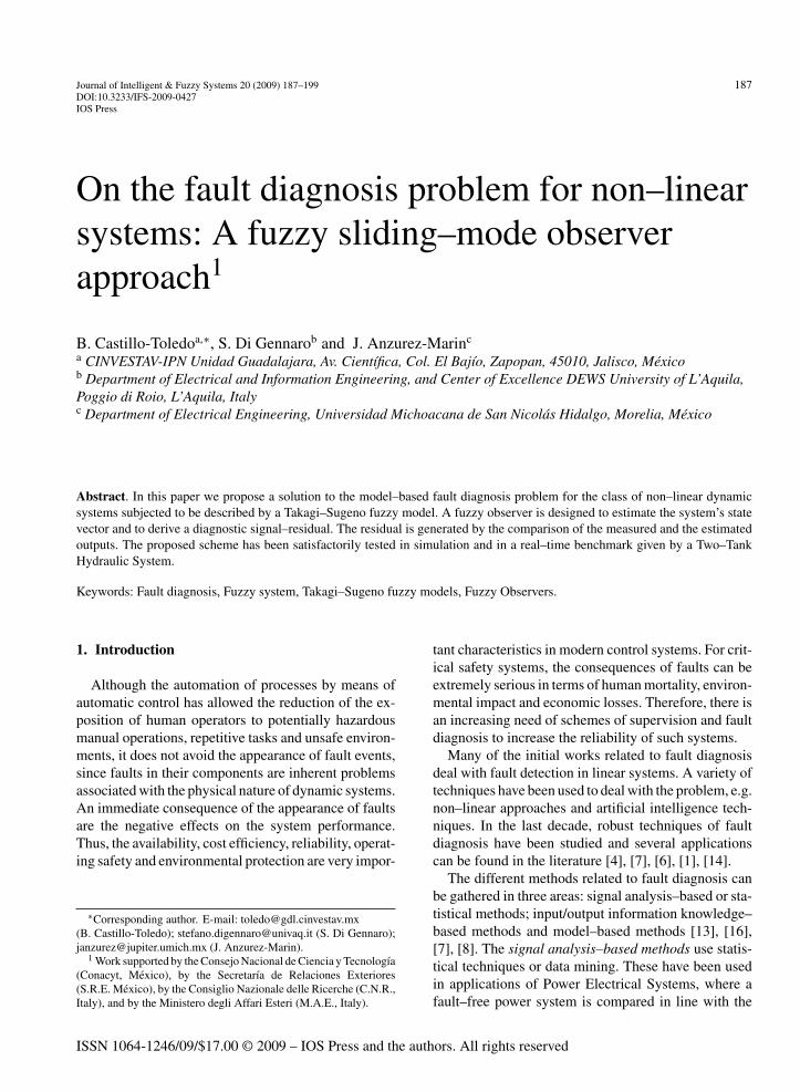
A structure commonly accepted for the model–basedfault diagnosis is shown in Figure 1. In this scheme,the residual generation subsystem provides a diagnos-tic signal, the residual, which depends only on the faults

Fig. 1. General structure of the model–based fault diagnosis

and not on the inputs, while in the decision making sub-system, the residuals are examined regarding the likeli-hood of a fault. A decision rule is then applied to deter-mine if the fault appears. A threshold value is generallyused to guarantee robustness.

Most of the model–based fault diagnosis methodsare based on linear system models and, traditionally,the fault diagnosis problem for non–linear dynamicsystems is analyzed in two steps: first, the model islinearized around a desired operating point, and thena specific linear technique is applied to generate adiagnostic signal, e.g. Kalman filters, observers, parityrelations, parameter estimation, etc. [4], [11]. However,since the behavior of many engineering systems ex-hibits nonlinearities, nonlinear models are more likelyto be necessary for FDI purpose, since linear modelsare only valid in a local region around an equilibriumpoint. Motivated by this reason, in the last years manyefforts have been made for the use of non–linear systemtechniques for fault diagnosis. For nonlinear systems,one difficulty results from the presence of non mea-sured states, and two different approaches for dealingwith this problem have been proposed, namely elimina-tion and estimation. The estimation, through dynamicalobservers, has been addressed for example in [9], [17],[12], among many others. In particular, in [10] a decou-pling strategy for a non–linear system is used to deriveseveral subsystems, containing information about spe-cific faults of the system in consideration. Once thesesubsystem are determined, a Luenberger fuzzy observeris implemented to generate the residuals. Parametricvariations are not considered in this approach. In [6] afuzzy observer is used to reconstruct the fault, ratherthan to detect its appearance through a residual signal.On the other hand, the results presented in [1] involve afuzzy multiple observer, where the single componentsare fuzzy observers having the form presented in [19].This multiple observer is capable of reconstructing thestate and output vectors of a system, when some inputsare unknown. It is worth noting that, in this specificapproach, the fault information is not distinguishablethrough the residuals.

A fault diagnosis method using only output informa-tion could give incorrect information on the faults, whenthe inputs of the system change. A way to circumventthis problem, affecting the model–based fault diagnosismethods, is to use the residual–generation concept, inwhich the inputs and outputs are used to generate a faultindicator.

In this paper, we propose a model–based approachwith fuzzy observers in order to deal with the fault


B. Castillo-Toledo et al. / On the fault diagnosis problem for non–linear systems: A fuzzy sliding–mode observer approach 189

diagnosis problem. Roughly speaking, the proposed ap-proach consists of obtaining a Takagi–Sugeno fuzzymodel [18] of the non–linear system, and then design-ing fuzzy observers to estimate the system state vector.The diagnostic signal–residual is finally generated bythe comparison between the measured and the estimatedoutputs. This approach allows determining a diagnos-tic signal which is insensible to parametric variations ina neighborhood of the nominal parameter values, andsensible only to the fault signal.

The paper is organized as follows: In section 2 somebasic concepts on fault diagnosis theory, the problemdefinition and a way to solve it are shown. In section 3we describe an application example. In section 4 we re-port the simulation and experimental results, and finallyin section 5 we present some conclusions.

2. Observer–based fault diagnosis

In general, a fault will be considered as a change inthe behavior of the system due to external inputs ex-ceeding the limits of a pre-specified tolerance. There-fore, the fault diagnosis concept will be referred to asthe problem of detecting and locating the fault, namely,not only merely recognize the presence of a fault, butalso identify on which component of the system thefault has appeared. This is formally defined as the FaultDetection and Isolation (FDI) problem.

A traditional approach to fault diagnosis is basedon hardware redundancy methods, which use multi-ple range sensors, actuators, computers and software tomeasure and/or control a particular variable. It is possi-ble however to use different measured values and theircombinations instead of duplicating each componentindividually to smooth the conflict between the relia-bility and the cost due to the additional components.This is the concept defined as functional or analyticalredundancy or model based approach, because it takesadvantage of the redundant analytical relationships be-tween several measured variables in the monitored pro-cess [11].

The major advantage of the model–based approachis that no additional hardware is needed in order toperform the fault detection and identification algo-rithm since the analytical redundancy uses a mathemat-ical model of the original system. The resulting signalr(t) = y(t)− y(t) generated from the comparison of themeasured and the estimated outputs is called symptomor residual. The absolute value of this residual shouldbe close enough to zero when the system is in normal

operating condition, namely should enter in a finite timeTB a ball BB of radius B of the origin, while should di-verge from zero, and leaveBB in finite time, when a faultf (t) occurs in the system. Therefore, this property ofthe residual can be used to determine whether or not anabnormal behavior should be considered as a fault [5],[8], i.e. the residual must satisfy the following condition

|r(t)|≈ 0 if f (t) = 0 (normal operation)

|r(t)|� 0 if f (t) �= 0 (faulty operation).

We say that the residual is sensitive to a specific set offaults. In this sense, a desirable property of the residualis to be insensitive or robust to parametric variations ina neighborhood of the nominal values, namely, theseparametric variations should not be confused with afault.

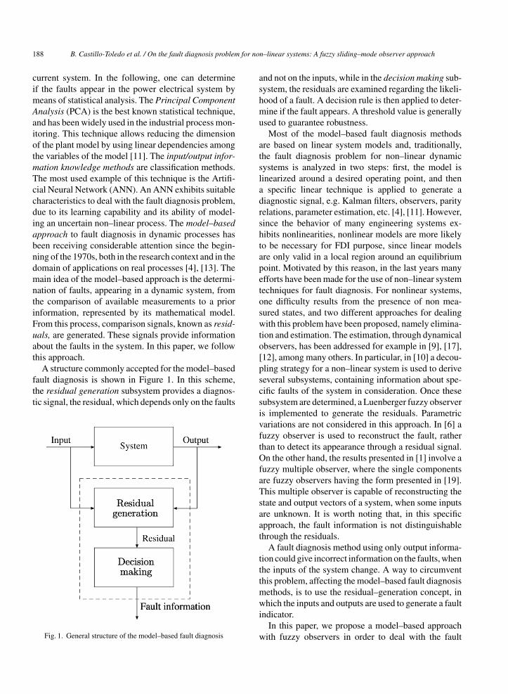
Figure 1 shows that an essential problem in themodel–based FDI is the generation of the diagnosticsignal–residual, because if the algorithm that generatesthe residuals is not correctly designed, important in-formation about the faults could be lost. This has moti-vated the study and proposal of different methods for theresiduals generation, like Kalman filters, Luenbergerobservers and fuzzy observers [11]. In particular, theobserver–based approach consists of the appropriateconstruction of an observer of the states of the system,generally in a fault–free situation, which provides anestimation of the output of the system that is comparedwith the measured output in order to generate the resid-uals to be used to detect a fault. The residual generationscheme is depicted in Figure 2. The basic idea is to elim-inate every input component from the output so that theoutput depends only on the component related to thefault, i.e., to construct a fuzzy observer which providesa desirable estimation of the output of the system, to

Fig. 2. Residual generation scheme with fuzzy observer



generate a residual which allows the proper identifica-tion of the fault and its localization by means of somesuitable algorithm.

As discussed previously, the model–based approachneeds a mathematical model of the system to be ob-served. In the case of non–linear dynamic systems, thedesign of observers is not in general an easy task dueto the nonlinearities of the model. Several approacheshave been proposed to deal with this important prob-lem. One of the recent approaches consists of achievingan approximation of the non–linear system behavior interms of an aggregation of linear dynamics calculatedaround some interesting points in the state–space, andthen calculate an observer for each linear submodel. Inthis context, the Takagi–Sugeno (TS) fuzzy modelingprovides a systematic way of obtaining a set of linearmodels that describe, at least locally, the behavior ofthe nonlinear dynamics [18].

In the following we develop a method based on outputfuzzy observers. These observers are very useful andhave several advantages, among which the possibilityof working with reduced observation error dynamics, afinite time convergence for all the observable states androbustness under parameter variations. More precisely,let us consider nonlinear system described by

x = f (x, u, d, µ)

y = h(x, µ)(1)

where x(t) ∈ IRn is the state of the system, u(t) ∈ IRm

is the input signal, d(t) ∈ IRq is an unknown input vec-tor usually containing external disturbances or signalsreflecting faults affecting the system, y(t) ∈ IRm is ameasurable output signal, and µ ∈ IRν is a vector of thesystem parameters subject to change.

The TS fuzzy model is described by a set of fuzzy IF–THEN rules which represent local linear input–outputrelations of a non–linear system. The main feature ofa TS fuzzy model is the ability of expressing the localdynamic of each fuzzy implication (rule) by a linearsubsystem [18]. In other words, suppose that it is pos-sible to describe locally the input–output behavior ofsystem (1) by a TS fuzzy dynamic model described bythe following r rules

Plant rule i:

IF z1 is M1i and · · · and zp is Mpi

THEN Σi:

{x = Aix + Biu + Eid + δi

yi = Cix + ∆i, i = 1, · · · , r

where z1, · · · , zp are measurable premise variableswhich may coincide with some states or a combina-tion of them, δi, ∆i are functions due to the vari-ation of the parameter vector µ with respect to thenominal value µ0, Ai, Bi, Ei, Ci are the nomi-nal matrices, i.e. corresponding to µ = µ0, Mji

are the fuzzy sets and the linear subsystems are ob-tained from some knowledge of the dynamics on theprocess.

For a given triplet (x, u, d), the aggregate fuzzymodel is obtained by using a singleton fuzzifier, prod-uct inference and center of gravity defuzzifier, resultingin the following description

x =r∑

i=1

ωiAix +r∑

i=1

ωiBiu +r∑

i=1

ωiEid +r∑

i=1

ωiδi

y =r∑

i=1

ωiCix +r∑

i=1

ωi∆i

(2)

where ωi is the normalized weight for each rule calcu-lated from the membership functions for zj in Mji andsatisfying ωi = ωi(z) ≥ 0 and

r∑i=1

ωi(z) = 1 (3)

with z = (z1 · · · zp

)T .For this system, we can formulate the Observed–

Based Fault Detection and Isolation Problem (OFDIP)which consists of finding an observer

ξ = γ(ξ, u, y)

y = θ(ξ)

such that the absolute values of the residuals convergein a finite time TB to a ball BB of radius B of theorigin, when the system is in normal operating con-dition, while leave BB in finite time when a fault oc-curs in the system. Moreover, the residuals have tobe insensitive to parametric variations in a neighbor-hood of the nominal values of the parameters of thesystem. In the following section we will determinesuch an observer considering a family of sliding modeobservers.



2.1. Sliding mode fuzzy observers for theTakagi–Sugeno model

According to the previous section we note that therequirement of observability of the nonlinear system isa necessary condition for generating the residuals. Tak-ing advantage of the TS description of the dynamics ofthis nonlinear system, we will assume that it is possibleto construct local observers for each linear subsystem.This motivates the following assumptions.

(H1) The pairs (Ci, Ai), i = 1, · · · , r, are detectable.�

(H2) There exist δmax, ∆max such that ‖δi‖ ≤ δmax,‖∆i‖ ≤ ∆max, for each i = 1, · · · , r. �

We propose the design of an aggregate sliding modefuzzy observer structure based on local fuzzy observers,with each local observer associated with each fuzzy rulegiven as

Observer rule i:

IF z1 is M1i and · · · and zp is Mpi

THEN Σi:

{ξ = Aiξ + Biu + Li(y − y) + ϕi

y = Ciξ, i = 1, · · · , r

where ϕi is a discontinuous vector to be determinedlater on. We assume also that the premise variables donot depend on the estimated state variables.

We use the idea of the Parallel Distributed Compen-sation (PDC) proposed in [18], where the overall stateestimation is a combination of individual local observeroutputs. The overall observer dynamics will be then aweighted sum of individual linear observers, namely

ξ =r∑

i=1

ωiAiξ +r∑

i=1

ωiBiu +r∑

i=1

ωiLi(y − y) +r∑

i=1

ωiϕi

y =r∑

i=1

ωiCiξ (4)

where the weights are the same as those used in theaggregate fuzzy model of the nonlinear system (2). Toanalyze the convergence of the fuzzy observer, the stateestimation error is defined as e = x−ξ. Using (2) and (4)we get

e =r∑

i=1

r∑j=1

ωiωjAije +r∑

i=1

ωi

[Eid + δi − ϕi

]

−r∑

i=1

r∑j=1

ωiωjLi∆j (5)

with Aij = Ai − LiCj . The convergence of the estima-tion error is expressed in the following result.

Theorem 2.1. Consider the TS fuzzy model (2), andsuppose that there exist positive definite matrices Ni, Fi

and P satisfying the following linear matrix inequalities(LMI’s)

ATi P + PAi − CT

i NTi − NiCi < 0, i = 1, · · · , n

ATi P + PAi − CT

j NTi − NiCj + AT

j P + PAj − CTi NT

j − NjCi < 0, i < j ≤ r.

(6)

Then, under (H1), (H2), if the faulty signal d satisfiesthe condition of normal operation

‖d‖ ≤ db (7)

then there exists a sliding mode fuzzy observer (4), with

ϕi =

⎧⎪⎨⎪⎩

k‖Ei‖P−1CT Ce

‖Ce‖ if‖Ce‖ > ε

k‖Ei‖P−1CT Ceε if‖Ce‖ ≤ ε

(8)

ε > 0 fixed, C =r∑

i=1ωiCi, ‖Ce‖ = ‖y − y‖,

k = Dmax2κminε

> 0, Dmax = κmax‖Λ−1‖d2b + ‖Λ−1

δ ‖δ2max + κ∆,max‖Λ−1

∆ ‖∆2max

κmin = mini=1,···,r

‖Ei‖, κmax = maxi=1,···,r

‖Ei‖2, κ∆,max = maxi=1,···,r

‖Li‖2(9)

guaranteeing practical convergence of the estimationerror in finite time

TB = t0 + ln(

rδC

B‖e0‖

)1/α

, r =√

λPmax

λPmin

, δC =r∑

i=1

‖Ci‖

(10)



where t0 is the initial time instant, λPmin, λP

max are theminimum and maximum eigenvalue of P , with estima-tion output error bound

B = rε + ∆max. (11)

If the faulty signal d violates the normal operation con-dition (7), then estimation error exits the ball BB infinite time and the residual detection is activated. �Proof. Let us consider the following Lyapunov candi-date function V = eT Pe, with P = PT > 0. Derivingthis function and using (5) we get

V =r∑

i=1

r∑j=1

ωiωjeT (PAij + AT

ijP)e

+ 2r∑

i=1

ωi

[eT PEid + eT Pδi − eT Pϕi

]

− 2r∑

i=1

r∑j=1

ωiωjeT PLi∆j. (12)

In the following we use the Young inequality

XT Y + YT X ≤ XT ΛX + YT Λ−1Y

for matrices X, Y ∈ IRn×k, and Λ ∈ IRk×k, Λ = ΛT >

0 [21]. Hence, from (12) one gets

V ≤r∑

i=1

r∑j=1

ωiωj eT (PAij + ATijP)e

+ eT P(Λ + Λδ + Λ∆)Pe

+r∑

i=1

ωidT ET

i Λ−1Eid +r∑

i=1

ωTi δiΛ

−1δ δi

+r∑

i=1

r∑j=1

ωiωj∆Tj LT

i Λ−1∆ Li∆j

− 2eT P

r∑i=1

ωiϕi (13)

Λ, Λδ, Λ∆ symmetric and positive definite. Under (H1)and setting Li = P−1Ni, by (6) the first term on theright–hand side of equation (13) is negative definite.Let us set

ATi P + PAi − CT

i NTi − NiCi = −Qij

with Qij = QTij > 0 thanks to the first of (6).

Let us consider first the case of system normal oper-ation, in which the faulty signal d satisfies (7). Setting

λ = γmin − ρ, ρ = ‖P(Λ + Λδ + Λ∆)P‖with γmin = min

i,j=1,···,rλ

Qij

min, λQij

min the minimum eigen-

value of Qij , using (3), from (13) one works out

V ≤ −λ‖e‖2 + Dmax − 2eT P

r∑i=1

ωiϕi

where (H2) and (9) have been used. Note that one canfix the matrices Λ, Λδ, Λ∆ so that ρ < γmin.

We have now to distinguish two cases, due to the factthat the observer (4) may determine an error e such that‖Ce‖ > ε or ‖Ce‖ ≤ ε. In the first case, choosing thefunctions ϕi as in (8), for ε < ‖Ce‖ ≤ ‖C‖‖e‖

V ≤ −λ‖e‖2 + Dmax − 2k

r∑i=1

ωi‖Ei‖eT CT Ce

‖Ce‖≤ −λ‖e‖2 + Dmax − 2kκminε = −λ‖e‖2.

Therefore, using standard arguments [15], for ‖e‖ >

ε/‖C‖ one obtains that the error satisfies

‖e‖ ≤ r

(‖e0‖e−α(t−t0) + ε

‖C‖

)where α = λ/(2λP

max), e0 is the error at time t0. Hence,during the normal operation and under bounded pa-rameter variations, the error is uniformly ultimatelybounded with bound b = rε/‖C‖, i.e. one obtains thepractical convergence of the estimation error. It is easyto check that the estimation error enters the ball of radiusb in a finite time tb = t0 + ln(‖C‖‖e0‖/ε)1/α. Note that‖C‖‖e0‖/ε > 1. Finally, from (2), (4) and using (H3)

‖Ce‖ = ‖y − y‖ =∥∥∥∥∥

r∑i=1

ωiCie +r∑

i=1

ωi∆i

∥∥∥∥∥≤ r

(‖C‖‖e0‖e−α(t−t0) + ε

)+ ∆max

namely, during the normal operation and under boundedparameter variations, Ce = y − y is uniformly ulti-mately bounded with bound (11), after a finite time

TB = t0 + ln

(r‖C‖

rε + ∆max

‖e0‖)1/α

≤ t0

+ ln

(rδC

rε + ∆max

‖e0‖)1/α

= TB, ‖C‖ ≤ δC



and hence after a finite time (10). Note that TB > t0for ∆max < r(δC‖e0‖− ε) (recall that here we consider‖e0‖ > ε/‖C‖ > ε/δC). This means that the maximalparameter variation has to be small enough so that theball BB does not contain the point e0.

In the second case, when ‖Ce‖ ≤ ε, taking ϕi asin (8)

V ≤ −λ‖e‖2 + Dmax − 2k

r∑i=1

ωi‖Ei‖eT CT Ce

ε

≤ −λ‖e‖2 + Dmax − 2kκmin‖Ce‖2

ε

= − (1 − ϑ)λ‖e‖2

+ Dmax

ε2

[ε2 − eT

(CT C + ε2ϑλ

Dmax

Im×m

)e

]

≤ −(1 − ϑ)λ‖e‖2

for ‖e‖≥ ε√λR

max

, with ϑ ∈ (0, 1), and λRmax the maxi-

mum eigenvalue of the matrix

R = CT C + ε2ϑλ

Dmax

Im×m.

Therefore, during the normal operation and underbounded parameter variations, the error e is uniformlyultimately bounded with bound b′ = rε/

√λR

max ≤ b,

as well as the output error Ce = y − y is uniformly ul-timately bounded with bound B′ = r ε‖C‖/√λR

max +∆max ≤ B, since ‖C‖/√λR

max ≤ 1.In conclusion, in both cases ‖Ce‖ > ε, ‖Ce‖ ≤

ε the estimation output error remains bounded withbound (11) during the normal operation. During faultyoperation, condition (7) is violated, and the convergenceanalysis is not valid anymore, and it is not possible toensure that the error enters or remains in the ball BB,and the fault can be detected after a finite time (10). �

Remark. The proof of this theorem allows the con-struction of the fuzzy observer (4). As clear from theproof, the design parameters are be used to determine asuitable bound db for the the external signal signal d(t)in order to be considered a fault. Moreover, if we con-sider that d(t) can also take into account variations inthe system parameters, it is clear that the observer (4) isrobust against bounded parameter variations satisfyingthe normal parameter operation. �

3. Model–based fault detection for two–tankhydraulic system

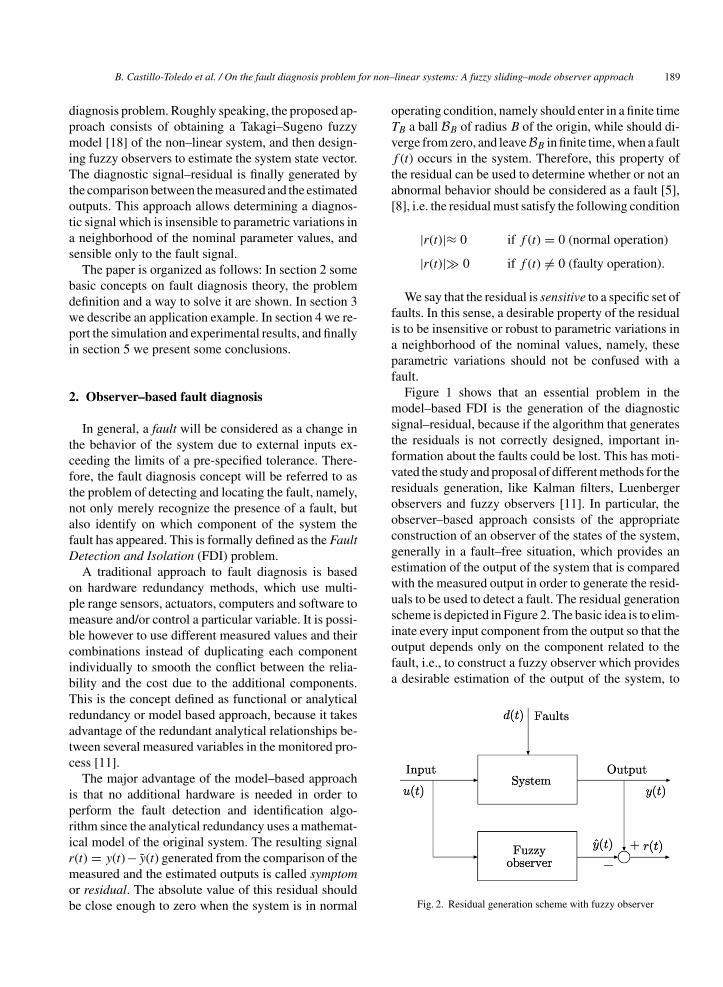
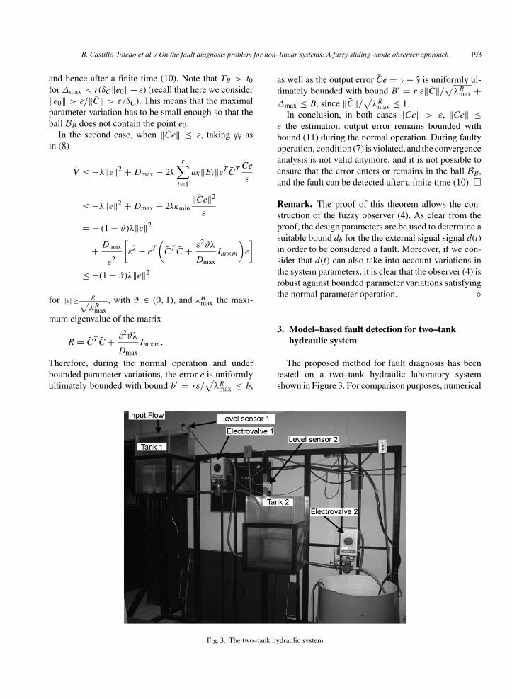
The proposed method for fault diagnosis has beentested on a two–tank hydraulic laboratory systemshown in Figure 3. For comparison purposes, numerical

Fig. 3. The two–tank hydraulic system



simulations have been carried out using the mathemat-ical model of the system, and real–time experimentshave been performed on the laboratory system. Thissystem consists of two interconnected tanks, two ultra-sonic level sensors, two industrial electro–valves con-nected at the output of the tanks and a pump providingconstant supply rate.

The hydraulic system has as inputs the voltage sup-plied to each one of the electro–valves, and as outputsthe liquid levels of each tank. The mathematical modelof the system is described by [2]

h1 = 1

At

(φe − w1

√(1 + fs1)h1

)

h2 = 1

At

(w1

√(1 + fs1)h1 − w2

√(1 + fs2)h2

)

w1 = 1

τ(ke1v1 − w1)

w2 = 1

τ(ke2v2 − w2) (14)

where hi, wi and vi, i = 1, 2, are the liquid level in theith tank, the opening ratio of the ith electro–valve, andthe voltage input to the ith electro–valve, respectively;At is the transversal area of each tank; τ, ke1, ke2 are thetime constant and the static gains of the electro–valvesrespectively; φe is a constant input flow to the tank 1and fs1 and fs2 model the faults in the level sensors 1and 2, respectively.

For this system, we have considered faults in both thelevel sensors, and the proposed method has been tested.

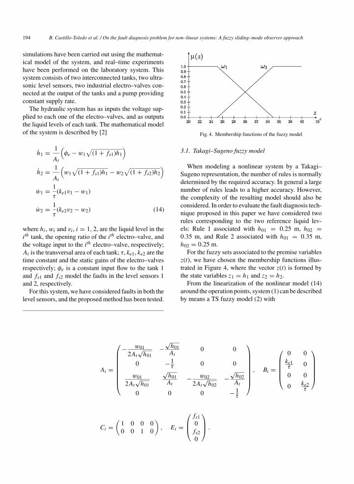
Fig. 4. Membership functions of the fuzzy model

3.1. Takagi–Sugeno fuzzy model

When modeling a nonlinear system by a Takagi–Sugeno representation, the number of rules is normallydetermined by the required accuracy. In general a largenumber of rules leads to a higher accuracy. However,the complexity of the resulting model should also beconsidered. In order to evaluate the fault diagnosis tech-nique proposed in this paper we have considered tworules corresponding to the two reference liquid lev-els: Rule 1 associated with h01 = 0.25 m, h02 =0.35 m, and Rule 2 associated with h01 = 0.35 m,h02 = 0.25 m.

For the fuzzy sets associated to the premise variablesz(t), we have chosen the membership functions illus-trated in Figure 4, where the vector z(t) is formed bythe state variables z1 = h1 and z2 = h2.

From the linearization of the nonlinear model (14)around the operation points, system (1) can be describedby means a TS fuzzy model (2) with

Ai =

⎛⎜⎜⎜⎜⎜⎜⎜⎝

− w01

2At

√h01

−√

h01At

0 0

0 −1τ 0 0

w01

2At

√h01

√h01At

− w02

2At

√h02

−√

h02At

0 0 0 −1τ

⎞⎟⎟⎟⎟⎟⎟⎟⎠

, Bi =

⎛⎜⎜⎜⎜⎝

0 0ke1τ 0

0 0

0 ke2τ

⎞⎟⎟⎟⎟⎠

Ci =(

1 0 0 00 0 1 0

), Ei =

⎛⎜⎝

fs10

fs20

⎞⎟⎠ .



Taking now T = 2.6525 s, At = 0.16 m2 and thefollowing set of parameters for each operation points(op1, op2)

op1 =(

h01 = 0.25 w01 = 0.20795 × 10−3 h02 = 0.35

w02 = 0.20795 × 10−3 ke1 = 0.03528 × 10−3 ke2 = 0.03923 × 10−3

)

op2 =(

h01 = 0.35 w01 = 0.17574 × 10−3 h02 = 0.25

w02 = 0.20795 × 10−3 ke1 = 0.03083 × 10−3 ke2 = 0.02860 × 10−3

)

we get

A1 =

⎛⎜⎝

−0.00129 −3.12500 0 00 −0.377 0 0

0.00129 3.125 −0.001290 −3.12500 0 0 −0.377

⎞⎟⎠ , B1 =

⎛⎜⎝

0 00.000013302 0

0 00 0.000014789

⎞⎟⎠

A2 =

⎛⎜⎝

−0.00092 −3.69754 0 00 −0.377 0 0

0.00092 3.69754 −0.00092 −3.697540 0 0 −0.377

⎞⎟⎠ , B2 =

⎛⎜⎝

0 00.000011624 0

0 00 0.000010783

⎞⎟⎠

C1 = C2 =(

1 0 0 00 0 1 0

), E1 =

⎛⎜⎝

1000

⎞⎟⎠ , E2 =

⎛⎜⎝

0010

⎞⎟⎠ .

The fuzzy observer (4) is designed to estimate thesystem output and generate the diagnostic signal–residual that indicates whether or not a fault appears.In this case two local observers are required in the ag-gregate fuzzy observer. With A1, A2, C1, C2, we solvethe LMI’s (6) and obtain N1, N2 and P , where the gainsLi are obtained from Li = P−1Ni, i = 1, 2, accordingwith Theorem 1.

Finally, the structured residual set [4] are designed tobe sensitive to a certain group of faults and insensitiveto others. The sensitivity and insensitivity propertiesmake the faults isolation possible. The ideal situation isto make each residual sensitive only to a particular faultand insensitive to all others. For example, system (14)is sensitive to certain faults (fs1, fs2 ) which cause thatthe diagnostic signal–residual to be active or not. Thisresponse pattern is known as fault signature or faultcode and is basically a characteristic of the faults inthe system [11]. For the hydraulic system, the responsepattern is shown in table 1. We observe that a fault insensor 1 will only activate the residual 1, and a fault insensor 2 will activate the residuals 1 and 3. Residuals 2and 4 correspond to faults (fw1, fw2) in the electro–valves 1 and 2, which are not studied here and therefore

in the fault signature matrix their diagnostic signal–residual is set to 0.

The fuzzy observer–based method has been tested inthe two–tank system both in simulation and real–time.The initial condition for the system has been chosen asx0 = (

0.25 0.0 0.25 0.0)T and has been carried

out around the operating point. In this work we haveconsidered the case when the sensor measurements areabruptly interrupted, due possibly to a sensor break-down.

3.2. Simulations

Using the TS fuzzy model and the proposed fuzzyobserver, the following three cases have been simulated

Table 1Fault signatures

FaultsResidual fs1 fs2 fw1 fw2 Notes:

r1 1 1 0 0 fs1 fault in sensor 1r2 0 0 0 0 fs2 fault in sensor 2r3 0 1 0 0 fw1 fault in actuator 1r4 0 0 0 0 fw2 fault in actuator 2



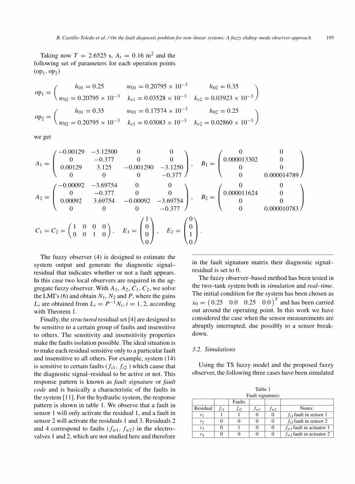
Fig. 5. Simulations: Residuals for a fault–free system

Case 1: Fault–free system. A 25 minutes running timehas been simulated. Figure 5 shows the re-sponse of the residuals for this case. As it canbe observed, the residuals have not been acti-vated, as expected, indicating that the systemis indeed free of faults.

Case 2: System with faults. Figure 6 shows the behaviorof residual signals 1 and 3 when an abrupt faultis introduced in sensor 1 at 10 minutes. As pre-dicted by the fault signature matrix, only the

Fig. 6. Simulations: Residuals corresponding to a fault in sensor 1

Fig. 7. Simulations: Residuals corresponding to a fault in sensor 2

residual 1 (r1) is activated. Note that the mag-nitude of the residual 3 is small, therefore wecan assume that the fault appears only in thesensor 1. In the same way, a fault in sensor 2has been simulated and the results in Figure 7show that the respective residual (r3) is acti-vated.

Case 3: Parametric variations. Here, parametricchanges on the values of Ai and Bi havebeen introduced. We observe in Figure 8 that

Fig. 8. Simulations: Residuals of a fault–free system withparametric variations



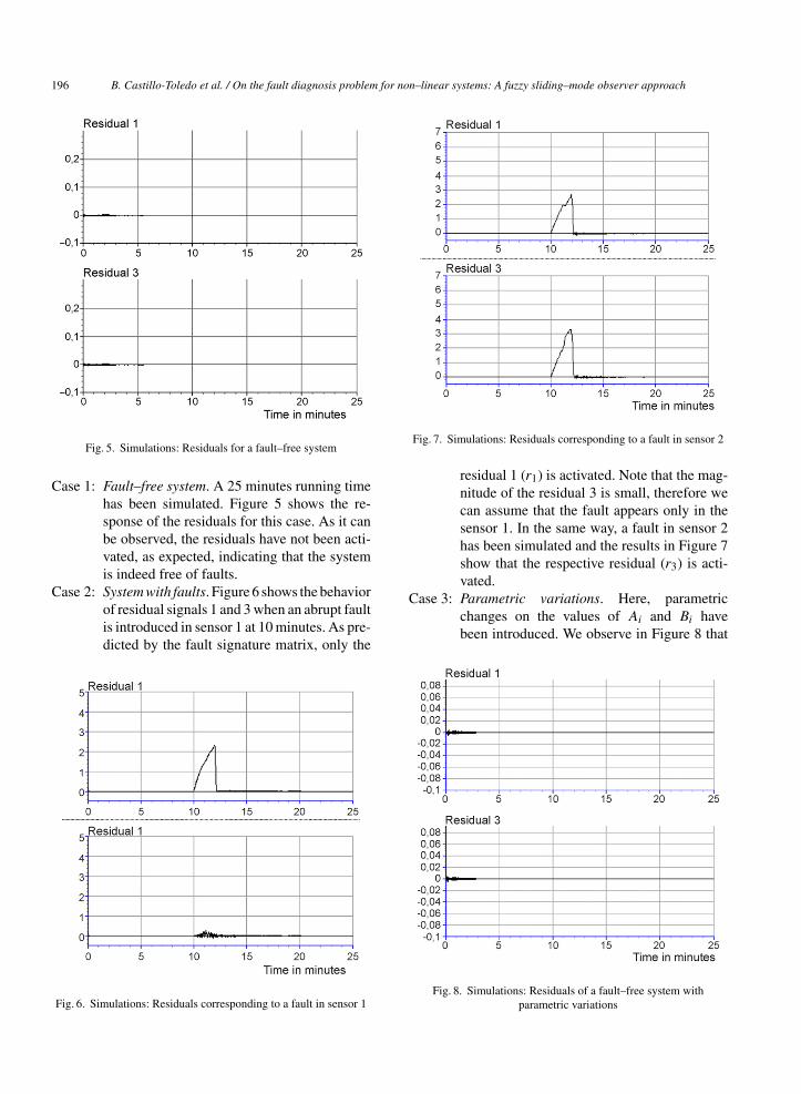
Fig. 9. Experimental results: Residuals of the fault–free two–tank system

Fig. 10. Experimental results: Residuals corresponding to a fault in sensor 1

none of the residuals are activated, showingthat the proposed scheme is robust in face ofparametric variations in a neighborhood ofthe nominal values. This is in accordance withTheorem 1, as already explained in Remark 1.

3.3. Experimental results

We have reproduced in the experimental setup thethree cases taken into account in the simulation section.In the case of fault–free, the residuals have not been ac-

tivated while the system operates in normal conditions,as shown in Figure 9.

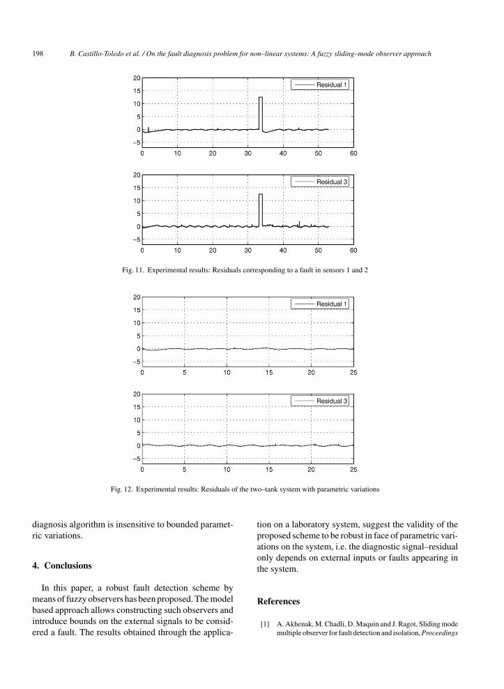
In the second case, faults in sensors 1 and 2 have beendetermined by disconnecting them for a short period.Figures 10 and 11 show that the respective residualsactivate correctly, allowing the correct detection of thefault.

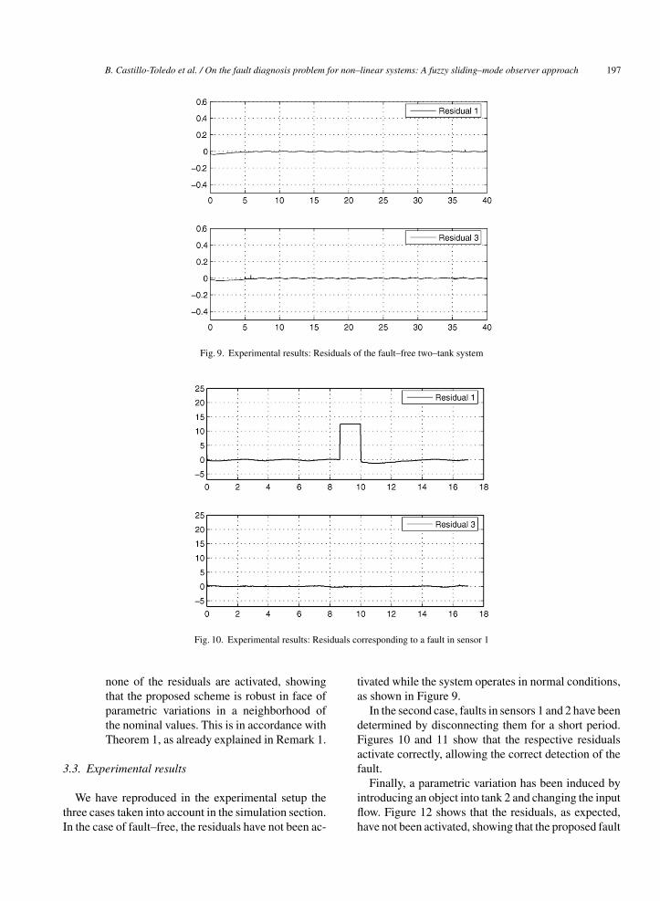
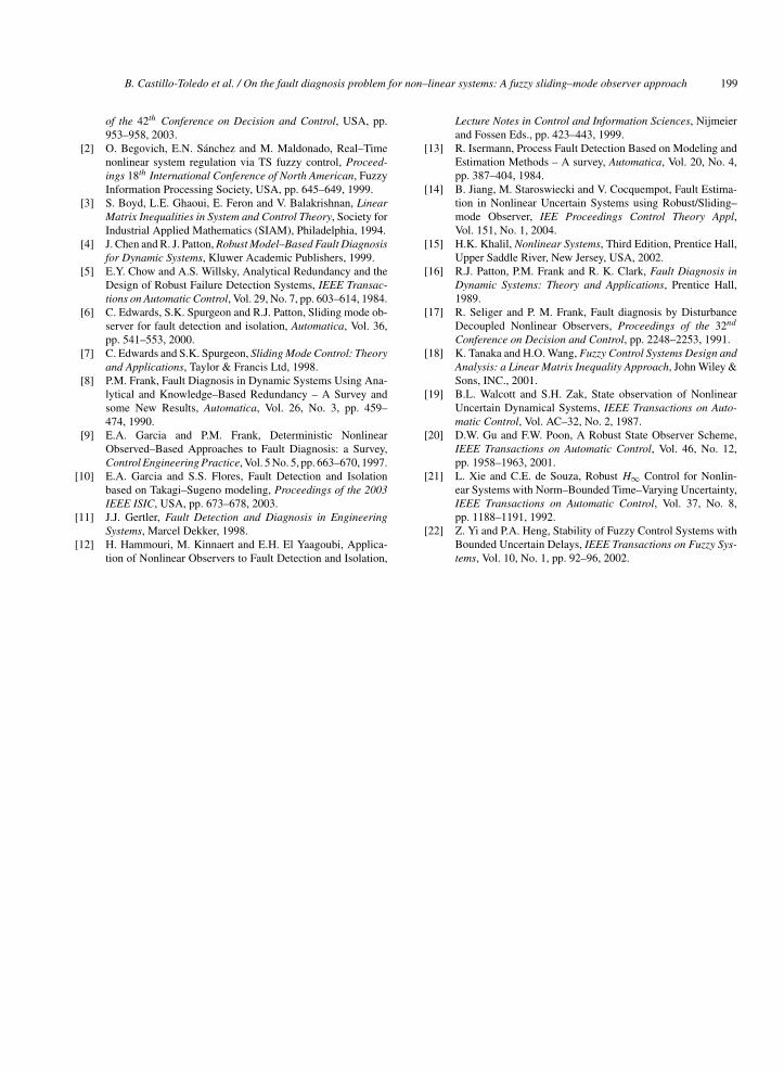
Finally, a parametric variation has been induced byintroducing an object into tank 2 and changing the inputflow. Figure 12 shows that the residuals, as expected,have not been activated, showing that the proposed fault



Fig. 11. Experimental results: Residuals corresponding to a fault in sensors 1 and 2

Fig. 12. Experimental results: Residuals of the two–tank system with parametric variations

diagnosis algorithm is insensitive to bounded paramet-ric variations.

4. Conclusions

In this paper, a robust fault detection scheme bymeans of fuzzy observers has been proposed. The modelbased approach allows constructing such observers andintroduce bounds on the external signals to be consid-ered a fault. The results obtained through the applica-

tion on a laboratory system, suggest the validity of theproposed scheme to be robust in face of parametric vari-ations on the system, i.e. the diagnostic signal–residualonly depends on external inputs or faults appearing inthe system.

References

[1] A. Akhenak, M. Chadli, D. Maquin and J. Ragot, Sliding modemultiple observer for fault detection and isolation, Proceedings



of the 42th Conference on Decision and Control, USA, pp.953–958, 2003.

[2] O. Begovich, E.N. Sanchez and M. Maldonado, Real–Timenonlinear system regulation via TS fuzzy control, Proceed-ings 18th International Conference of North American, FuzzyInformation Processing Society, USA, pp. 645–649, 1999.

[3] S. Boyd, L.E. Ghaoui, E. Feron and V. Balakrishnan, LinearMatrix Inequalities in System and Control Theory, Society forIndustrial Applied Mathematics (SIAM), Philadelphia, 1994.

[4] J. Chen and R. J. Patton, Robust Model–Based Fault Diagnosisfor Dynamic Systems, Kluwer Academic Publishers, 1999.

[5] E.Y. Chow and A.S. Willsky, Analytical Redundancy and theDesign of Robust Failure Detection Systems, IEEE Transac-tions on Automatic Control, Vol. 29, No. 7, pp. 603–614, 1984.

[6] C. Edwards, S.K. Spurgeon and R.J. Patton, Sliding mode ob-server for fault detection and isolation, Automatica, Vol. 36,pp. 541–553, 2000.

[7] C. Edwards and S.K. Spurgeon, Sliding Mode Control: Theoryand Applications, Taylor & Francis Ltd, 1998.

[8] P.M. Frank, Fault Diagnosis in Dynamic Systems Using Ana-lytical and Knowledge–Based Redundancy – A Survey andsome New Results, Automatica, Vol. 26, No. 3, pp. 459–474, 1990.

[9] E.A. Garcia and P.M. Frank, Deterministic NonlinearObserved–Based Approaches to Fault Diagnosis: a Survey,Control Engineering Practice, Vol. 5 No. 5, pp. 663–670, 1997.

[10] E.A. Garcia and S.S. Flores, Fault Detection and Isolationbased on Takagi–Sugeno modeling, Proceedings of the 2003IEEE ISIC, USA, pp. 673–678, 2003.

[11] J.J. Gertler, Fault Detection and Diagnosis in EngineeringSystems, Marcel Dekker, 1998.

[12] H. Hammouri, M. Kinnaert and E.H. El Yaagoubi, Applica-tion of Nonlinear Observers to Fault Detection and Isolation,

Lecture Notes in Control and Information Sciences, Nijmeierand Fossen Eds., pp. 423–443, 1999.

[13] R. Isermann, Process Fault Detection Based on Modeling andEstimation Methods – A survey, Automatica, Vol. 20, No. 4,pp. 387–404, 1984.

[14] B. Jiang, M. Staroswiecki and V. Cocquempot, Fault Estima-tion in Nonlinear Uncertain Systems using Robust/Sliding–mode Observer, IEE Proceedings Control Theory Appl,Vol. 151, No. 1, 2004.

[15] H.K. Khalil, Nonlinear Systems, Third Edition, Prentice Hall,Upper Saddle River, New Jersey, USA, 2002.

[16] R.J. Patton, P.M. Frank and R. K. Clark, Fault Diagnosis inDynamic Systems: Theory and Applications, Prentice Hall,1989.

[17] R. Seliger and P. M. Frank, Fault diagnosis by DisturbanceDecoupled Nonlinear Observers, Proceedings of the 32nd

Conference on Decision and Control, pp. 2248–2253, 1991.[18] K. Tanaka and H.O. Wang, Fuzzy Control Systems Design and

Analysis: a Linear Matrix Inequality Approach, John Wiley &Sons, INC., 2001.

[19] B.L. Walcott and S.H. Zak, State observation of NonlinearUncertain Dynamical Systems, IEEE Transactions on Auto-matic Control, Vol. AC–32, No. 2, 1987.

[20] D.W. Gu and F.W. Poon, A Robust State Observer Scheme,IEEE Transactions on Automatic Control, Vol. 46, No. 12,pp. 1958–1963, 2001.

[21] L. Xie and C.E. de Souza, Robust H∞ Control for Nonlin-ear Systems with Norm–Bounded Time–Varying Uncertainty,IEEE Transactions on Automatic Control, Vol. 37, No. 8,pp. 1188–1191, 1992.

[22] Z. Yi and P.A. Heng, Stability of Fuzzy Control Systems withBounded Uncertain Delays, IEEE Transactions on Fuzzy Sys-tems, Vol. 10, No. 1, pp. 92–96, 2002.

Documents

On the fault diagnosis problem for non–linear systems: A ...ing.univaq.it/digennaro/Ricerca/I24.pdf · Introduction Although the ... Many of the initial works related to fault diagnosis