HAL Id: hal-00462117https://hal-polytechnique.archives-ouvertes.fr/hal-00462117

Submitted on 8 Mar 2010

HAL is a multi-disciplinary open accessarchive for the deposit and dissemination of sci-entific research documents, whether they are pub-lished or not. The documents may come fromteaching and research institutions in France orabroad, or from public or private research centers.

L’archive ouverte pluridisciplinaire HAL, estdestinée au dépôt et à la diffusion de documentsscientifiques de niveau recherche, publiés ou non,émanant des établissements d’enseignement et derecherche français ou étrangers, des laboratoirespublics ou privés.

On the existence and uniqueness of a solution to theinterior transmission problem for

piecewise-homogeneous solidsCédric Bellis, B. B. Guzina

To cite this version:Cédric Bellis, B. B. Guzina. On the existence and uniqueness of a solution to the interior transmissionproblem for piecewise-homogeneous solids. Journal of Elasticity, Springer Verlag, 2010, in press. hal-00462117

Journal of Elasticity manuscript No.(will be inserted by the editor)

On the existence and uniqueness of a solution to the interiortransmission problem for piecewise-homogeneous solids

Cedric Bellis · Bojan B. Guzina

Received: date / Accepted: date

Abstract The interior transmission problem (ITP), which plays a fundamental role in in-verse scattering theories involving penetrable defects, is investigated within the frameworkof mechanical waves scattered by piecewise-homogeneous, elastic or viscoelastic obstaclesin a likewise heterogeneous background solid. For generality, the obstacle is allowed to bemultiply connected, having both penetrable components (inclusions) and impenetrable parts(cavities). A variational formulation is employed to establish sufficientconditions for theexistence and uniqueness of a solution to the ITP, provided that the excitation frequencydoes not belong to (at most) countable spectrum of transmission eigenvalues. The featuredsufficient conditions, expressed in terms of the mass density and elasticity parameters of theproblem, represent an advancement over earlier works on thesubject in that i) they posea precise, previously unavailable provision for the well-posedness of the ITP in situationswhen both the obstacle and the background solid are heterogeneous, and ii) they are di-mensionally consistent i.e. invariant under the choice of physical units. For the case of aviscoelastic scatterer in an elastic solid it is further shown, consistent with earlier studiesin acoustics, electromagnetism, and elasticity that the uniqueness of a solution to the ITPis maintained irrespective of the vibration frequency. When applied to the situation whereboth the scatterer and the background medium are viscoelastic i.e. dissipative, on the otherhand, the same type of analysis shows that the analogous claim of uniqueness does not hold.Physically, such anomalous behavior of the “viscoelastic-viscoelastic” case (that has eludedprevious studies) has its origins in a lesser known fact thatthe homogeneous ITP is notmechanically insulated from its surroundings – a feature that is particularly cloaked in situa-tions when either the background medium or the scatterer aredissipative. A set of numericalresults, computed for ITP configurations that meet the sufficient conditions for the existenceof a solution, is included to illustrate the problem. Consistent with the preceding analy-sis, the results indicate that the set of transmission values is indeed empty in the “elastic-viscoelastic” case, and countable for “elastic-elastic” and “viscoelastic-viscoelastic” config-urations.

Keywords interior transmission problem· transmission eigenvalues· piecewise-homogeneous media· anisotropic viscoelasticity· existence· uniqueness

Cedric BellisDepartment of Civil Engineering, University of Minnesota,Minneapolis, MN 55455, USA;Laboratoire de Mecanique des Solides (UMR CNRS 7649), Ecole Polytechnique, Palaiseau, France.E-mail: bellis@lms.polytechnique.fr

Bojan GuzinaDepartment of Civil Engineering, University of Minnesota,Minneapolis, MN 55455, USA.E-mail: guzina@wave.ce.umn.edu

2

1 Introduction

Over the past two decades mathematical theories of inverse scattering have, to a large de-gree, experienced a paradigm shift, most notably through the development of the so-calledqualitative or sampling methods [5] for non-iterative obstacle reconstruction from remotemeasurements of the scattered field. These techniques, which provide a powerful alternativeto the customary minimization approaches and weak-scatterer approximations, are com-monly centered around the development of an indicator function, that varies with coordi-nates of the interior sampling point, and projects remote observations of the scattered fieldonto a suitable functional space synthesizing the “baseline” wave motion inside the back-ground (i.e. obstacle-free) domain. Such indicator function is normally designed to reachextreme values when the sampling point “falls” inside the support of the hidden scatterer,thereby providing an computationally-effective platformfor geometric obstacle reconstruc-tion. Among the diverse field of sampling methods [41,18], one may mention thelinearsampling method[15,14] and thefactorization method[27] among the most prominent ex-amples. In the context of penetrable scatterers (e.g. elastic inclusions within the frameworkof mechanical waves), these theories have exposed the need to study and understand a non-traditional boundary value problem, termed theinterior transmission problem(ITP), wheretwo bodies with common support are subjected to a prescribedjump in Cauchy data betweentheir boundaries. Covered by no classical theory, this problem has been the subject of earlyinvestigations since late 1980’s [16,44]. The critical step in studying the ITP involves deter-mination of conditions (in terms of input parameters) underwhich the problem is well-posedin the sense of Hadamard. Invariably, this leads to the analysis of the interior transmissioneigenvalues, i.e. frequencies for which the homogeneous ITP permits a non-trivial solution.In particular, the characterization of such eigenvalue sethas become of key importance inrecent studies [40,26].

So far, two distinct methodologies have been pursued to investigate the well-posednessof the ITP, mainly within the context of Helmholtz and Maxwell equations. On the one hand,integral equation-type formulations have been developed in [16,44] for scalar-wave prob-lems, and later adapted to deal with electromagnetic waves [23,25]. One the other hand,starting from the seminal work in [24], an alternative treatment of the ITP has been devel-oped in [6] that involves a customized variational formulation combined with the compactperturbation argument. This approach has since been successfully applied in a series of pa-pers to a variety of acoustic and electromagnetic scattering problems, see e.g. [7,8].

In the context of elastic waves, investigation of the ITP hasbeen spurred by the in-troduction of the linear sampling method for far-field [1,12] and near-field [39,2,38,22]inverse scattering problems, as well as the development of the factorization method for elas-todynamics [13]. To date, the elastodynamic ITP has been investigated mainly within theframework established for the Helmholtz and Maxwell equations, notably via integral equa-tion approach [12] for homogeneous dissipative scatterers, and the variational treatment [10]for heterogeneous, anisotropic, and elastic scatterers ina homogeneous elastic background.Recently, a method combining integral equation approach and compact perturbation argu-ment has been proposed in [11] for homogeneous-isotropic elasticity to obtain sufficientconditions for the well-posedness of the ITP.

To extend the validity of the linear sampling and factorization methods to a wider andmore realistic class of inverse scattering problems, the focus of this study is the ITP forsituations where both the obstacle and the background solidare piecewise-homogeneous,anisotropic, and either elastic or viscoelastic. This typeof heterogeneity concerning thebackground solid has particular relevance to e.g. seismic imaging and non-destructive ma-

3

terial testing where layered configurations are common, as created either via natural depo-sition or the manufacturing process. For generality, the obstacle is allowed to be multiplyconnected, having both penetrable components (inclusions) and impenetrable parts (cavi-ties). In this setting, emphasis is made on the well-posendess of the visco-elastodynamicITP, and in particular on the sufficient conditions under which the set of interior transmissioneigenvalues is either countable or empty. For an in-depth study of the problem, a variationalapproach that generalizes upon the results in [6] and [10] isdeveloped, including a treat-ment of the less-understood “viscoelastic-viscoelastic”case where both the obstacle and thebackground solid are dissipative. The key result of the proposed developments are the suf-ficient conditions under which the ITP involving piecewise-homogeneous, anisotropic, andviscoelastic solids is well-posed provided that the excitation frequency does not belong to(at most) countable spectrum of transmission eigenvalues.These conditions aim to over-come some of the limitations of the earlier treatments in (visco-) elastodynamics in that:i) they pose a precise, previously unavailable provision for the well-posedness of the ITP insituations when the obstacle and the background solid are both heterogeneous, and ii) theyare dimensionally consistent i.e. invariant under the choice of physical units.

2 Preliminaries

Consider a piecewise-homogeneous, “background” viscoelastic solidΩ ⊂ R3 (not neces-

sarily bounded and isotropic) composed ofN homogeneous regular regionsΩn. Assum-ing time-harmonic motion with implicit factoreiωt and making reference to the correspon-dence principle [21], letρ> 0 and C denote respectively the piecewise-constant mass den-sity and (complex-valued) viscoelasticity tensor characterizing Ω. For clarity, all quanti-ties appearing in this study are interpreted asdimensionlessfollowing the scaling schemein Table 1 whered0 is the characteristic length,κ0 is the reference elastic modulus, andρ0 is the reference mass density. Without loss of generality,ρ0 can be taken such thatinfρ(x) : x∈Ω = 1, leaving the choice ofκ0 at this point arbitrary.

Table 1: Scaling scheme

Dimensionless quantity ScaleMass density ρ ρ0

Viscoelasticity tensor, traction vector C, t κ0

Displacement and position vectors u,x d0Vibration frequency ω d−1

0

√

κ0/ρ0

Next, letΩ be perturbed by a bounded obstacleD⊂Ω composed ofM∗ homogeneousviscoelastic inclusionsDm

∗ andMo disconnected cavitiesDjo. In this setting one may write

D = D∗∪Do, whereD∗ =⋃M∗

m=1 Dm∗ andDo =

⋃Moj=1 D

jo. Here it is assumed that the

cavities are separated from inclusions i.e.D∗∩Do = ∅, and thatΩ\Do is connected. Similarto the case of the background solid, the viscoelasticity tensorC∗ and mass densityρ∗ > 0

characterizingD∗ are understood in a piecewise-constant sense. For the purpose of thisstudy, the reference lengthd0 appearing in Table 1 can be taken asd0 = |D|1/3, i.e. as thecharacteristic obstacle size.

4

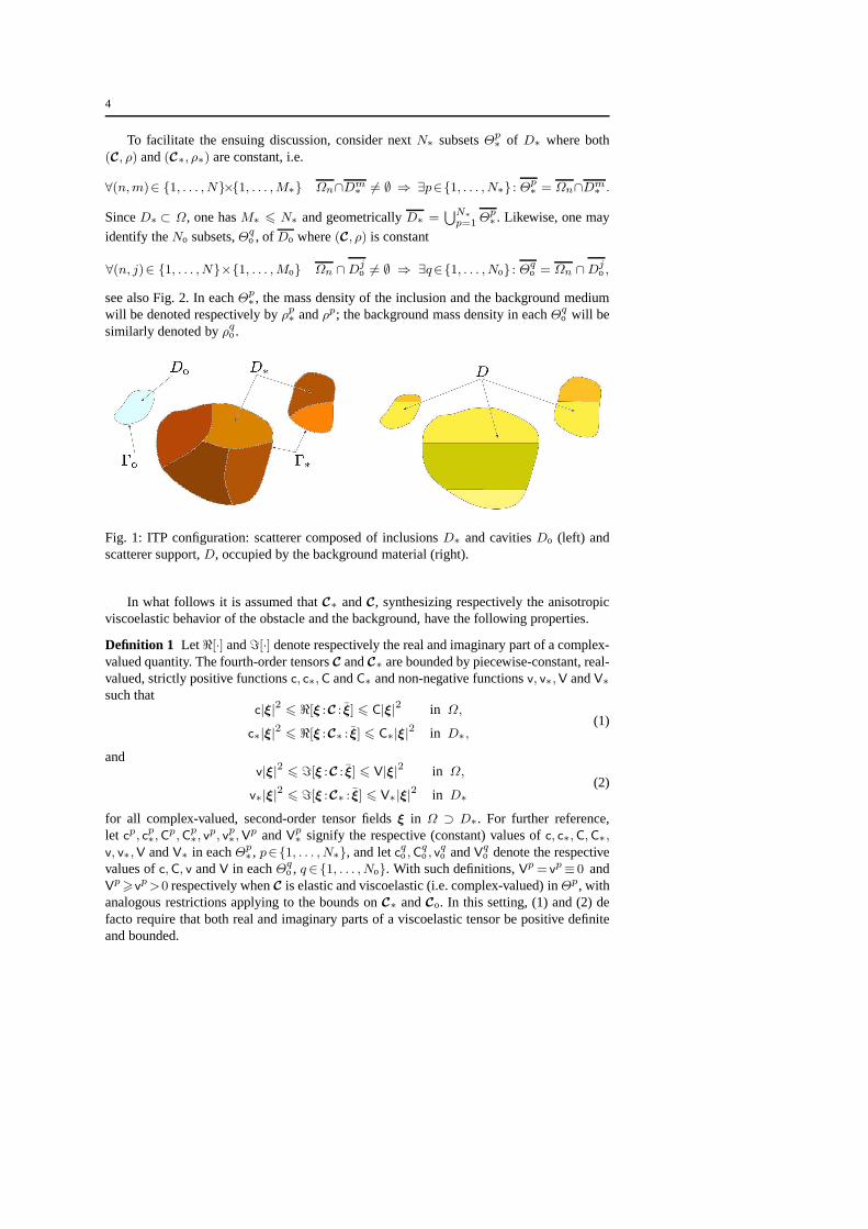
To facilitate the ensuing discussion, consider nextN∗ subsetsΘp∗ of D∗ where both

(C, ρ) and(C∗, ρ∗) are constant, i.e.

∀(n,m)∈ 1, . . . , N×1, . . . ,M∗ Ωn∩Dm∗ 6= ∅ ⇒ ∃p∈1, . . . , N∗ : Θ

p∗ = Ωn∩Dm

∗ .

SinceD∗ ⊂ Ω, one hasM∗ 6 N∗ and geometricallyD∗ =⋃N∗

p=1 Θp∗ . Likewise, one may

identify theNo subsets,Θqo , of Do where(C, ρ) is constant

∀(n, j)∈ 1, . . . , N×1, . . . ,Mo Ωn ∩Djo 6= ∅ ⇒ ∃q∈1, . . . , No : Θ

qo = Ωn ∩Dj

o ,

see also Fig. 2. In eachΘp∗ , the mass density of the inclusion and the background medium

will be denoted respectively byρp∗ andρp; the background mass density in eachΘqo will be

similarly denoted byρqo.

Fig. 1: ITP configuration: scatterer composed of inclusionsD∗ and cavitiesDo (left) andscatterer support,D, occupied by the background material (right).

In what follows it is assumed thatC∗ andC, synthesizing respectively the anisotropicviscoelastic behavior of the obstacle and the background, have the following properties.

Definition 1 Letℜ[·] andℑ[·] denote respectively the real and imaginary part of a complex-valued quantity. The fourth-order tensorsC andC∗ are bounded by piecewise-constant, real-valued, strictly positive functionsc, c∗,C andC∗ and non-negative functionsv, v∗,V andV∗

such thatc|ξ|2 6 ℜ[ξ :C : ξ] 6 C|ξ|2 in Ω,

c∗|ξ|26 ℜ[ξ :C∗ : ξ] 6 C∗|ξ|

2 in D∗,(1)

andv|ξ|2 6 ℑ[ξ :C : ξ] 6 V|ξ|2 in Ω,

v∗|ξ|26 ℑ[ξ :C∗ : ξ] 6 V∗|ξ|

2 in D∗

(2)

for all complex-valued, second-order tensor fieldsξ in Ω ⊃ D∗. For further reference,let cp, cp∗,C

p,Cp∗, v

p, vp∗,Vp andVp

∗ signify the respective (constant) values ofc, c∗,C,C∗,

v, v∗,V andV∗ in eachΘp∗ , p∈1, . . . , N∗, and letcqo,C

qo, v

qo andVq

o denote the respectivevalues ofc,C, v andV in eachΘq

o , q∈1, . . . , No. With such definitions,Vp = vp≡ 0 and

Vp>v

p>0 respectively whenC is elastic and viscoelastic (i.e. complex-valued) inΘp, withanalogous restrictions applying to the bounds onC∗ andCo. In this setting, (1) and (2) defacto require that both real and imaginary parts of a viscoelastic tensor be positive definiteand bounded.

5

Comment.With reference to the result in [34] which establishes the major symmetry of a(tensor) relaxation function by virtue of the Onsager’s reciprocity principle [45] , it followsthatC∗ andC have the usual major and minor symmetries whereby

ℜ[ξ :C : ξ] = ξ : ℜ[C] : ξ, ℜ[ξ :C∗ : ξ] = ξ : ℜ[C∗] : ξ,

ℑ[ξ :C : ξ] = ξ : ℑ[C] : ξ, ℑ[ξ :C∗ : ξ] = ξ : ℑ[C∗] : ξ.(3)

One may also note that the imposition of the upper bounds,C,C∗,V andV∗ in (1) and (2) isjustified by the boundedness of the moduli comprisingC andC∗, whereasc, c∗, v andv∗ en-sure thermomechanical stability of the system [36,20]. These upper and lower bounds can beshown to signify the extreme eigenvalues of (the real and imaginary parts of) a fourth-orderviscoelasticity tensor, defined with respect to a second-order eigentensor. Explicit treatmentof such eigenvalue problems is difficult in a general anisotropic case, which may featureup to six distinct eigenvalues per real and imaginary part. In the isotropic case, however,tensorsC andC∗ can be synthesized in terms of the respective (complex) shear moduli µandµ∗, and bulk moduliK andK∗. Under such restriction,C andC∗ have only two distincteigenvalues [28], given respectively by2µ, 3K and2µ∗, 3K∗. Depending on the signof the real parts of the underlying Poisson’s ratiosν andν∗ [42], these moduli satisfy therelationships

0 < ℜ[ν] < 12 ⇒ C = 3ℜ[K] > 2ℜ[µ] = c,

− 1 < ℜ[ν] < 0 ⇒ C = 2ℜ[µ] > 3ℜ[K] = c,

0 < ℜ[ν∗] <12 ⇒ C∗ = 3ℜ[K∗] > 2ℜ[µ∗] = c∗,

− 1 < ℜ[ν∗] < 0 ⇒ C∗ = 2ℜ[µ∗] > 3ℜ[K∗] = c∗.(4)

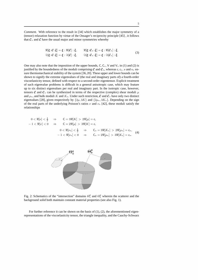
Fig. 2: Schematics of the “intersection” domainsΘp∗ andΘq

o wherein the scatterer and thebackground solid both maintain constant material properties (see also Fig. 1).

For further reference it can be shown on the basis of (1), (2),the aforementioned eigen-representations of the viscoelasticity tensor, the triangle inequality, and the Cauchy-Schwarz

6

inequality that∣

∣

∣

∣

∫

Θp∗

ξ : C∗ : η dx

∣

∣

∣

∣

6 (C∗+ V∗) ||ξ||L2(Θp∗)

||η||L2(Θp∗),

∣

∣

∣

∣

∫

Θp∗

ξ : C : η dx

∣

∣

∣

∣

6 (C+ V) ||ξ||L2(Θp∗)

||η||L2(Θp∗),

∣

∣

∣

∣

∫

Θqo

ξ : C : η dx

∣

∣

∣

∣

6 (C+ V) ||ξ||L2(Θqo ) ||η||L2(Θq

o ),

(5)

whereξ andη are square-integrable, complex-valued, second-order tensor fields inΘp∗ and

Θqo , p∈1, . . . , N∗, q∈1, . . . , No.

3 Interior transmission problem

Consider the time-harmonic scattering of viscoelastic waves at frequencyω where the so-called free fielduF, namely the displacement field that would have existed in theobstacle-free domainΩ, is perturbed (scattered) by a bounded obstacleD=D∗∪Do ⊂Ω describedearlier. This boundary value problem can be conveniently written as

∇·[C∗ :∇u∗] + ρ∗ω2u∗ = 0 in D∗, (6a)

∇·[C :∇u] + ρω2u = 0 in Ω\D, (6b)

u∗ = u+ uF on∂D∗, (6c)

t∗[u∗] = t[u] + t[uF] on ∂D∗, (6d)

t[u] + t[uF] = 0 on ∂Do (6e)

whereu∗ is the (total) displacement field within piecewise-homogeneous inclusionD∗; uis the so-called scattered field signifying theperturbationof uF in Ω\D due to the presenceof the scatterer;t∗[ϑ] = C∗ :∇ϑ ·n and t[ϑ] = C :∇ϑ ·n refer to the surface tractions on∂D; ∇ implies differentiation “to the left” [32], andn is the unit normal on the boundaryof D oriented toward its exterior. Here (6a) is to be interpretedas a short-hand notation forthe set ofM∗ governing equations applying over the respective homogeneous regionsDm

∗

(m=1, . . .M∗), supplemented by the continuity of displacements and tractions across∂Dm∗

where applicable. Analogous convention holds in terms of (6b) strictly applying over openhomogeneous regionsΩn\D.

In what follows, it is assumed that the boundary ofΩ (if any) is subject to Robin-typeconditions whereby (6) are complemented by

λ(I2−N)·u+N ·t[u] = 0 on ∂Ω, (7)

whereλ > 0 is a constant;n, implicit in the definition oft[u], is oriented outward fromΩ; andN is a suitable second-order tensor that varies continuouslyalong smooth piecesof ∂Ω. Note that (7) include homogeneous Dirichlet (N ≡ 0) and Neumann (N ≡ I2)boundary conditions as special cases. In situations whereΩ is unbounded (e.g. a half-space),(6) and (7) are completed by the generalized radiation condition [31], namely

limR→∞

∫

ΓR

[

t[u](x) · U(x,y)− u(x) · T(x,y)]

dx = 0, ∀y ∈ Ω, (8)

whereΓR = SR ∩ Ω; SR is a sphere of radiusR centered at the origin;U denotes thedisplacement Green’s tensor for the obstacle-free solidΩ, andT is the traction Green’stensor associated withU.

7

Interior transmission problem.With reference to the direct scattering framework (6)–(8),henceforth referred to as the transmission problem (TP), investigation of the associatedin-verse scatteringproblem in terms of the linear sampling and factorization methods [15,12,22,27,13] leads to the analysis of the so-called interior transmission problem (ITP) [5]. Inthe context of the present study, the ITP can be stated as the task of finding an elastodynamicfield that solves thecounterpartof (6) where the support of (6b), namelyΩ\D, is replacedby D. Previous studies have, however, shown that the analysis ofan ITP is complicated bytheloss of ellipticityrelative to its “mother” TP that is well known to be elliptic.An in-depthstudy of this phenomenon can be found in [19] who showed, making reference to acousticwaves, that the ITP is not elliptic at any frequency. Here it is also useful to recall that theTP (6)–(8) and the associated ITP can both be represented by acommon set of boundaryintegral equations (written over∂D), which leads to the well-known phenomenon of fic-titious frequencies [4,30,43] plaguing the boundary integral treatment of direct scatteringproblems.

For a comprehensive treatment of the problem, the ITP associated with (6)–(8) is nextformulated in a general setting which i) allows for the presence of body forces, and ii) in-terprets the interfacial conditions over∂D∗ as a prescribed jump in Cauchy data betweenu

andu∗. Making reference to Fig. 1 and the basic concepts of functional analysis [35], suchgeneralized ITP can be conveniently stated as a task of finding (u∗,u,uo) ∈ H1(D∗) ×H1(D∗)×H1(Do) satisfying

∇·[C∗ :∇u∗] + ρ∗ω2u∗ = f∗ in D∗, (9a)

∇·[C :∇u] + ρω2u = f in D∗, (9b)

∇·[C :∇uo] + ρω2uo = f in Do, (9c)

u∗ = u+ g on∂D∗, (9d)

t∗[u∗] = t[u] + h∗ on∂D∗, (9e)

t[uo] = ho on∂Do, (9f)

whereHk ≡ W k,2 denotes the usual Sobolev space;(f∗,f) ∈ L2(D∗)×L2(D); g ∈

H1

2 (∂D∗); (h∗,ho)∈ H− 1

2 (∂D∗)×H− 1

2 (∂Do), and

t∗[u∗] = C∗ :∇u∗ ·n ∈ H− 1

2 (∂D∗),

t[u] = C :∇u·n ∈ H− 1

2 (∂D∗), (10)

t[uo] = C :∇uo·n ∈ H− 1

2 (∂D∗).

For completeness, it is noted that (9a)–(9c) and (9d)–(10) are interpreted respectively in thesense of distributions and the trace operator whilef∗ andf , signifying the negatives of bodyforces, are placed on the right-hand side to facilitate the discussion.

Definition 2 Values ofω for which the homogeneous ITP, defined by setting(f∗,f , g,h∗,ho) =

(0,0, 0,0,0) in (9), has a non-trivial solution are calledtransmission eigenvalues.

8

Modified interior transmission problem.To deal with anticipated non-ellipticity of the fea-tured ITP, it is next useful to consider the compact perturbation of (9) as

∇·[C∗ :∇u∗]− ρ∗u∗ = f∗ in D∗ (11a)

∇·[C :∇u]− ρu = f in D∗ (11b)

∇·[C :∇uo]− ρuo = f in Do (11c)

u∗ = u+ g on∂D∗ (11d)

t∗[u∗] = t[u] + h∗ on∂D∗ (11e)

t[uo] = ho on∂Do, (11f)

see also [6] in the context of the acoustic waves. To demonstrate the compact nature of suchperturbation, one may introduce the auxiliary space

Ξ(D) :=

(u∗,u,uo) ∈ H1(D∗)×H1(D∗)×H1(Do) :

∇·[C∗ :∇u∗] ∈ L2(D∗), ∇·[C :∇u] ∈ L2(D∗), ∇·[C :∇uo] ∈ L2(Do)

, (12)

and a differential-trace operatorM representing (11) fromΞ(D) into L2(D∗)×L2(D∗)×

L2(Do)×H1

2 (∂D∗)×H− 1

2 (∂D∗)×H− 1

2 (∂Do) such that

M(u∗,u,uo) :=(

∇·[C∗ :∇u∗]−ρ∗u∗, ∇·[C :∇u]−ρu, ∇·[C :∇uo]−ρuo,

(u∗−u)|∂D∗, (t∗[u∗]−t[u])|∂D∗

, t[uo]|∂Do

)

(13)

wheret andt∗ are defined as in (10). On the basis of (11) and (13), interior transmissionproblem (9) can be identified with operatorO ≡ M+(1+ω2)P from Ξ(D) intoL2(D∗)×

L2(D∗)×L2(Do)×H1

2 (∂D∗)×H− 1

2 (∂D∗)×H− 1

2 (∂Do), where the featured perturbationoperator

P(u∗,u,uo) :=(

ρ∗u∗, ρu, ρuo, 0, 0, 0)

(14)

is clearly compact by virtue of compact embedding ofH1(D∗) into L2(D∗) andH1(Do)

into L2(Do).

Definition 3 Triplet (u∗,u,uo) ∈ H1(D∗) × H1(D∗) × H1(Do) solving (11a)–(11c) inthe sense of distributions and (11d)–(11f) in the sense of the trace operator is called astrongsolutionof the modified ITP.

3.1 Weak formulation of the modified ITP

The next step is to examine the ellipticity of the modified ITP(11) through a variationalformulation, following the methodology originally introduced in [24] and later deployedin [6,10]. To this end, recall the definition of the “background” viscoelasticity tensor andconsider the space of symmetric second-order tensor fields

W (D∗) :=

Φ ∈ L2(D∗) : Φ = ΦT, ∇·Φ ∈ L2(D∗) and ∇× [C−1 :Φ] = 0

, (15)

equipped with the inner product

(Φ1,Φ2)W (D∗) := (Φ1,Φ2)L2(D∗) + (∇·Φ1,∇·Φ2)L2(D∗), (16)

9

and implied norm‖Φ‖2W (D∗) := ‖Φ‖2L2(D∗) + ‖∇·Φ‖2L2(D∗). (17)

For clarity it is noted that the curl operator in (15), definedas that “to the left” [32], is to beinterpreted in the weak sense. With reference to (11) and (15), let further E := H1(D∗) ×W (D∗)×H1(Do) and define the sesquilinear formA : E× E → C as

A(U, V ) :=

∫

D∗

[∇u∗ : C∗ :∇ϕ∗ + ρ∗u∗ · ϕ∗] dx+

∫

D∗

[

1

ρ(∇·U)·(∇·Φ) + U : C−1 :Φ

]

dx

+

∫

Do

[∇uo : C :∇ϕ+ ρuo · ϕ] dx−

∫

∂D∗

[

u∗ · Φ · n+ (U · n) · ϕ∗

]

dx,

(18)together with the antilinear formL : E → C

L(V ) :=

∫

D∗

1

ρf · (∇·Φ) dx−

∫

Do

f · ϕ dx−

∫

D∗

f∗ · ϕ∗ dx

+

∫

∂D∗

[

h∗ · ϕ∗ − g · Φ · n]

dx+

∫

∂Do

ho · ϕ dx,(19)

whereC denotes the complex plane,U=(u∗,U ,uo) ∈ E, andV =(ϕ∗,Φ,ϕ) ∈ E.With such definitions, one may recast (11) in a variational setting as a task of finding

U=(u∗,U ,uo) ∈ E such that

A(U, V ) = L(V ) ∀V =(ϕ∗,Φ,ϕ) ∈ E. (20)

Theorem 1 If problem (11) has unique strong solution(u∗,u,uo)∈H1(D∗)×H1(D∗)×H1(Do), then the variational problem (20) has unique weak solutionU=(u∗,C :∇u,uo)∈

E. Equally, if problem (20) has unique weak solutionU = (u∗,U ,uo) ∈ E, then modifiedITP (11) has unique strong solution(u∗,u,uo) ∈ H1(D∗)×H1(D∗)×H1(Do) such that(∇u+∇Tu)/2 = C

−1 :U .

Proof The proof of this theorem has two parts. The first part establishes that(u∗,u,uo)

solves (11) if and only if(u∗,U ,uo) solves (20), while the second part demonstrates theequivalence between the existence ofuniquesolutions.

Parity between the existence of solutions.

– Suppose that(u∗,u,uo) solves (11), and defineU = C : ∇u wherebyU ∈ W (D∗).By taking theL2(D∗) scalar product of (11a) withϕ∗ ∈ H1(D∗) and applying thedivergence theorem, one finds that

∫

D∗

[∇u∗ : C∗ :∇ϕ∗ + ρ∗u∗ · ϕ∗] dx−

∫

∂D∗

(U · n) · ϕ∗ dx =

∫

∂D∗

h∗ · ϕ∗ dx−

∫

D∗

f∗ · ϕ∗ dx, (21)

by virtue of the boundary condition (11e). Similarly, application of the divergence theo-rem to theL2(Do)-scalar product of (11c) withϕ∈H1(Do) yields

∫

Do

[∇uo : C :∇ϕ+ ρuo · ϕ] dx =

∫

∂Do

ho · ϕ dx−

∫

Do

f · ϕ dx. (22)

10

Finally, by taking theL2(D∗)-scalar product of (11b) withρ−1 ∇·Φ for someΦ ∈

W (D∗) and making use of (11d), one obtains

∫

D∗

[

1

ρ(∇·U) · (∇·Φ) + U : C−1 : Φ

]

dx−

∫

∂D∗

u∗ · Φ · n dx

=

∫

D∗

1

ρf · (∇·Φ) dx−

∫

∂D∗

g · Φ · n dx.(23)

The weak statement (20) is now recovered by summing (21)–(23), which demonstratesthatU = (u∗,U ,uo) ∈ E is indeed a solution of the variational problem.

– Conversely, letU = (u∗,U ,uo) ∈ E be a weak solution to (20). Since the hypothesis∇× [C−1:U ] = 0 guarantees thatC−1:U meets the strain compatibility conditions [32],there exists a functionu ∈ H1(D∗) such that(∇u+∇Tu)/2 = C

−1 : U in the senseof a distribution, defined up to a rigid-body motion. By virtue of the fact thatU solvesthe variational problem (20) for all(ϕ∗,Φ,ϕ) ∈ E, it follows by setting the triplet ofweighting fields respectively to(ϕ∗,0,0), (0,0,ϕ), and(0,Φ,0) that(u∗,u,uo) mustbe such that (21), (22) and (23) are satisfied independently.

By way of the divergence theorem, (21) yields

∫

D∗

(∇·[C∗ :∇u∗]− ρ∗u∗ − f∗) · ϕ∗ dx

+

∫

∂D∗

(h∗ + (C :∇u) · n− (C∗ :∇u∗) · n) · ϕ∗ dx = 0, ∀ϕ∗∈ H1(D∗)

whereby(u∗,u) satisfies

∇·[C∗ :∇u∗]− ρ∗u∗ = f∗ in D∗,

t∗[u∗] = t[u] + h∗ on∂D∗.(24)

Similarly, equality (22) leads to∫

Do

(∇·[C :∇uo]− ρuo− f)·ϕ dx +

∫

∂Do

(ho − C :∇uo · n)·ϕ dx = 0, ∀ϕ∈H1(Do)

which requires(u,uo) to satisfy

∇·[C :∇uo]− ρuo = f in Do,

t[uo] = ho on∂Do.(25)

On substitutingU = C :∇u in (23), on the other hand, it follows that for allΦ ∈ W (D∗)

∫

D∗

(

1

ρ∇·[C :∇u]− u−

1

ρf

)

·(∇·Φ) dx +

∫

∂D∗

(g + u− u∗) ·Φ ·n dx = 0. (26)

To deal with (26), it is convenient to introduce the “zero-mean and zero-first-order-moment” space of vector fields

L20(D∗) =

ϕ ∈ L2(D∗) :

∫

D∗

ϕ dx = 0,

∫

D∗

x× ϕ dx = 0

,

11

and to consider solutionχ ∈ H1(D∗) of the elastostatic problem

∇·[C :∇χ] = Λ in D∗, Λ ∈ L20(D∗),

C :∇χ · n = 0 on∂D∗.

By takingΦ = C :∇χ in (26) wherebyΦ ∈ W (D∗), ∇· Φ = Λ in D∗, andΦ · n = 0

on∂D∗, one finds that∫

D∗

(

1

ρ∇·[C :∇u]− u−

1

ρf

)

· Λ dx = 0 ∀Λ∈ L20(D∗),

and consequently, using identity(ω × x)·Λ = ω ·(x× Λ), that

1

ρ∇·[C :∇u]− u−

1

ρf = c+ ω × x in D∗, (27)

which specifiesu up to an rigid-body motion given by the translation vectorc and(infinitesimal) rotation vectorω.Consider next solutionχ ∈ H1(D∗) to the problem

∇·[C :∇χ] = 0 in D∗

C :∇χ · n = Λ on∂D∗, Λ∈ L20(∂D∗).

(28)

Again takingΦ = C :∇χ in (26), which this time impliesΦ ∈ W (D∗), ∇· Φ = 0 inD∗ andΦ · n = Λ on∂D∗, leads to

∫

∂D∗

(g + u− u∗) · Λ dx = 0 ∀Λ ∈ L20(∂D∗), (29)

so thatg + u− u∗ = c

′ + ω′ × x on∂D∗, (30)

wherec′ andω′ are vector constants.On substituting (27) and (30) into (26), one finds by virtue ofthe divergence theoremand identityω × x = Ω · x whereΩ≡ω × I that∫

∂D∗

[

(c+c′)+(ω+ω

′)×x]

·Φ·n dx +

∫

D∗

Ω : Φ dx = 0 ∀Φ ∈ W (D∗). (31)

Since the second integral vanishes due to the symmetry ofΦ and antisymmetry ofΩ,(31) requires thatc′ = −c and ω = −ω′. From (24), (25), (27) and (30), it nowimmediately follows that(u∗,u+ c+ ω × x) is a solution to (11).

Parity between the existence of unique solutions.

– Assume that problem (11) has a unique strong solution, and let U1 = (u1∗,U

1,u1o)

andU2 = (u2∗,U

2,u2o) denote two weak solutions to (20). By the equivalence be-

tween solutions to the two problems, one has that(u1∗,u

1,u1o) and(u2

∗,u2,u2

o), with(∇u1+∇Tu1)/2 = C

−1 : U1 and(∇u2+∇Tu2)/2 = C−1 : U2, are consequently solu-

tions to (11). Since the latter two triplets must coincide bypremise, it follows that thatu1∗= u2

∗, U1= U2 andu1

o = u2o, i.e. that the solution to the variational problem (20) is

likewise unique.

– Conversely, assume that (20) has a unique weak solution, andlet (u1∗,u

1,u1o) and

(u2∗,u

2,u2o) denote two strong solutions to (11). Since(u1

∗,C :∇u1,u1o) and(u2

∗,C :

∇u2,u2o) are consequently solutions to (20), one must haveu1

∗ = u2∗, ∇u1+∇Tu1 =

∇u2+∇Tu2 andu1o = u2

o by premise. The proof is completed by noting thatu1 andu2 are equal up to a rigid body motion, which must vanish thanks to the boundary con-dition (11d).

⊓⊔

12

4 Existence and uniqueness of a solution to the modified ITP

Having reduced the study of the modified ITP (11) to that of itsvariational statement (20),the question arises as to the conditions under which the latter problem is well-posed. Forclarity of exposition, the focus is made on thesufficientconditions that compare theelasticparameters of the inclusion, comprisingℜ[C∗], to those of the background in terms ofℜ[C].In general, it is possible that the consideration of material dissipation (synthesized viaℑ[C∗]

andℑ[C]) may relax the “elasticity” conditions under which (11) and(20) are elliptic, andthus help establish the sufficientand necessary conditions. The latter subject is, however,beyond the scope of this study. With such restraint, the following lemma helps establish thesufficient “elasticity” conditions.

Lemma 1 With reference to Definition 1 specifying the bounds on the viscoelastic tensorsC andC∗, the sesquilinear formA is elliptic if the inequalitiesρp< ρp∗ and C

p< cp∗ hold

in each “intersection” domainΘp∗ , p ∈ 1, . . . , N∗.

Proof ForU=(u∗,U ,uo) ∈ E, one finds from (18) that

A(U,U) =

∫

D∗

[∇u∗ : C∗ :∇u∗ + ρ∗u∗ · u∗] dx+

∫

D∗

[

1

ρ(∇·U ) · (∇·U) + U : C−1 : U

]

dx

+

∫

Do

[∇uo : C :∇uo + ρuo · uo] dx−

∫

∂D∗

[

u∗ · U · n+ (U · n) · u∗]

dx.

(32)On employing the divergence theorem, the triangle inequality, the Cauchy-Schwarz inequal-ity, and definition of the “intersection” domainsΘp

∗ , one finds

∣

∣

∣

∣

∫

∂D∗

ϕ∗ · Φ · n dx

∣

∣

∣

∣

6

N∗∑

p=1

[

‖ϕ∗‖L2(Θp∗)‖∇· Φ‖L2(Θp

∗)+ ‖∇ϕ∗‖L2(Θp

∗)‖Φ‖L2(Θp

∗)

]

.

(33)By virtue of the fact that|A(U,U)| > ℜ [A(U,U)], (33), and bounds (1) on (the real partsof) the viscoelasticity tensorsC∗ andC in eachΘp

∗ , it can be further shown that

|A(U,U)| >

N∗∑

p=1

[

cp∗‖∇u∗‖

2L2(Θp

∗)+ ρp∗‖u∗‖

2L2(Θp

∗)+

1

ρp‖∇· U‖2L2(Θp

∗)+

1

Cp ‖U‖2L2(Θp∗)

]

− 2

N∗∑

p=1

[

‖u∗‖L2(Θp∗)‖∇· U‖L2(Θp

∗)+ ‖∇u∗‖L2(Θp

∗)‖U‖L2(Θp

∗)

]

+

No∑

q=1

[

cqo‖∇uo‖

2L2(Θq

o )+ ρqo‖uo‖

2L2(Θq

o )

]

.

(34)Since for every(x, y) ∈ R

2, α > 0, andβ > 0 one has

αx2 +1

βy2 − 2xy =

α+ β

2

(

x−2

α+ βy

)2

+ (α− β)

(

1

2x2 +

1/β

α+ βy2)

, (35)

13

inequality (34) can be rewritten as

|A(U,U)| >

N∗∑

p=1

[

cp∗ + C

p

2

(

‖∇u∗‖L2(Θp∗)

−2

cp∗ + Cp

‖U‖L2(Θp∗)

)2

+ (cp∗ − Cp)

(

1

2‖∇u∗‖

2L2(Θp

∗)+

1/Cp

cp∗ + Cp

‖U‖2L2(Θp∗)

)

+ρp∗ + ρp

2

(

‖u∗‖L2(Θp∗)

−2

ρp∗ + ρp‖∇· U‖L2(Θp

∗)

)2

+ (ρp∗ − ρp)

(

1

2‖u∗‖

2L2(Θp

∗)+

1/ρp

ρp∗ + ρp‖∇· U‖2L2(Θp

∗)

)]

+

No∑

q=1

[

cqo‖∇uo‖

2L2(Θq

o )+ ρqo‖uo‖

2L2(Θq

o )

]

.

(36)

On introducing the lower-bound parameter

γ = minp=1,...,N∗

q=1,...,No

(

cp∗ − C

p

2,

cp∗ − C

p

Cp(cp∗ + Cp),ρp∗ − ρp

2,

ρp∗ − ρp

ρp(ρp∗ + ρp), cqo, ρ

qo

)

, (37)

one finds thatγ > 0 sinceρp < ρp∗ andCp < cp∗ in eachΘp

∗ by premise. On the basis of thisresult one finds, by dropping the “squared-difference” terms in (36), that

|A(U, U)| > γ

N∗∑

p=1

(

‖u∗‖2H1(Θp

∗)+ ‖U‖2W (Θp

∗)

)

+

No∑

q=1

‖uo‖2H1(Θq

o )

. (38)

Recalling thatU=(u∗,U ,uo) ∈ E, the sesquilinear formA is consequently elliptic with

|A(U,U)| > γ(

‖u∗‖2H1(D∗) + ‖U‖2W (D∗) + ‖uo‖

2H1(Do)

)

, (39)

which completes the proof.⊓⊔

One is now in position to investigate the variational formulation of the modified ITP.

Theorem 2 Under the assumptions of Lemma 1, variational problem (20) has a uniqueweak solutionU = (u∗,U ,uo) ∈ E with an a priori estimate

‖u∗‖H1(D∗) + ‖U‖W (D∗) + ‖uo‖H1(Do) 6

3C

γ

(

‖f∗‖L2(D) + ‖f‖L2(D∗) + ‖g‖H

1

2 (∂D∗)+ ‖h∗‖

H−1

2 (∂D∗)+ ‖ho‖

H−1

2 (∂Do)

)

, (40)

whereγ > 0 is given by (37), andC > 0 is a constant independent off∗, f , g, h∗ andho.

Proof The norm of the antilinear operatorL in (19) can be shown, by exercising the triangleinequality, the Cauchy-Schwarz inequality, the divergence theorem (applied toΦ) and thetrace theorem, to be continuous i.e. bounded with constantC > 0 independent off∗, f , g,h∗ andho such that

||L||E⋆ 6 C(

‖f∗‖L2(D) + ‖f‖L2(D∗)

+ ‖g‖H

1

2 (∂D∗)+ ‖h∗‖

H−1

2 (∂D∗)+ ‖ho‖

H−1

2 (∂Do)

)

, (41)

14

whereE⋆ denotes the dual ofE.To establish the boundedness of the sesquilinear formA(U, V ), on the other hand, one

may introduce the notation

||U ||2E := ‖u∗‖2H1(D∗) + ‖U‖2W (D∗) + ‖uo‖

2H1(Do),

||V ||2E := ‖ϕ∗‖2H1(D∗) + ‖Φ‖2W (D∗) + ‖ϕ‖2H1(Do),

(42)

for U, V ∈E defined as in (20). In this setting, it follows from (20), the triangle inequality,(5), the Cauchy-Schwarz inequality, (33), (42), and boundssuch as||∇u∗||L2(D∗) 6 ||U ||Ethat there is a constantC′>0 such that

|A(U, V )| 6 C′ ||U ||E ||V ||E. (43)

Using the notation introduced in (42), (39) can also be rewritten more compactly as

|A(U, U)| > γ ||U ||2E. (44)

With the boundedness (43) and coercivity (44) ofA now verified, the existence of a uniquesolution to the variational problem (20) follows directly from the Lax-Milgram theorem [35]which ensures that||U ||E 6 γ−1||L||E⋆ . In this setting, a priori estimate (40) is derived as aconsequence of (41), (42a), and upper bounds such as‖u∗‖H1(D∗) 6 ||U ||E.

⊓⊔

Theorem 3 Under the hypotheses of Lemma 1, modified ITP (11) has a uniquestrong so-lution (u∗,u,uo) ∈ H1(D∗)×H1(D∗)×H1(Do) with an a priori estimate

‖u∗‖H1(D∗) + ‖u‖H1(D∗) + ‖uo‖H1(Do) 6

c(

‖f∗‖L2(D) + ‖f‖L2(D∗) + ‖g‖H

1

2 (∂D∗)+ ‖h∗‖

H−1

2 (∂D∗)+ ‖ho‖

H−1

2 (∂Do)

)

, (45)

wherec > 0 is a constant independent off∗, f , g, h∗ andho.

Proof The first part of the claim, namely the existence and uniqueness of a strong solutionto (11) follow directly from Theorems 1 and 2, while inequality (45) can be obtained on thebasis of (11) and (40). In particular, from the relationshipU = C :∇u and the fact thatusatisfies (11b), it follows via triangle inequality that

‖u‖L2(D∗) 6 α(

‖U‖W (D∗) + ‖f‖L2(D∗)

)

, (46)

for some constantα > 0. By virtue of the bounds on the viscoelasticity tensorC in (1)and (2), on the other hand, one finds

‖∇u‖L2(D∗) = ‖C−1 : U‖L2(D∗) 6 β ‖U‖W (D∗), (47)

for someβ>0. On combining (46) and (47) to obtain theH1(D∗) norm ofu, estimate (45)follows directly as a consequence of (40) with

c 6

(

2 +√

α2(1+γ)2 + β2)

C

γ.

⊓⊔

15

5 Well-posedness of the ITP

Having established the conditions under which the modified problem (11) is uniquely solv-able, one is now in position to study the existence and uniqueness of a solution to the (orig-inal) ITP (9).

Theorem 4 Under the hypothesis thatρp< ρp∗ and Cp< c

p∗ in each “intersection” domain

Θp∗ , p ∈ 1, . . . , N∗ as in Lemma 1, the set of transmission eigenvaluesω ∈ C for which

the interior transmission problem (9) does not have a uniquesolution is either empty orforms a discrete set with infinity as the only possible accumulation point.

Proof With reference to the spaceΞ(D) introduced in (12), it is recalled that the modifiedITP (11) is represented by the differential-trace operatorM as in (13), while the originalproblem (9) is identified with operatorO= M + (1+ω2)P , whereP is the compact per-turbation given by (14). In Theorem 3 it is shown thatM−1 exists, and furthermore that itis bounded i.e. continuous under the assumptions of Lemma 1.Theorem 4 claims that theoperatorM+(1+ω2)P is invertible for allω ∈ C\S, whereS is either an empty set or adiscrete set of points in the complex planeC. SinceM−1 is continuous, this claim can beestablished by showing the analogous result for the operator

I + (1+ω2)M−1P ,

whereI is the identity operator fromΞ(D) into Ξ(D). As shown in Section 3, operatorPis compact owing to the compact embedding ofH1(D) into L2(D), and so isM−1P byvirtue of the continuity ofM−1 [35]. For this situation, the Fredholm alternative applies[47] whereby

(

I + (1+ω2)M−1P)−1

exists and is bounded except for, at most, adiscreteset of transmission eigenvaluesω ∈S ⊂ C (see also Definition 2). Finally, since the countable spectrum of (compact) operatorM−1P can only accumulate at zero [46],S is further characterized by infinity as the onlypossible accumulation point.

⊓⊔

5.1 Relaxed solvability criterion

With reference to Theorem 4, it is noted that the eigenvaluesof ITP (9) may form a countableset even in situations that violate the aforestated restriction: ρp < ρp∗ andCp < c

p∗ in each

Θp∗ , p ∈ 1, . . . , N∗. Indeed, the latter condition can be relaxed in a way similarto that

proposed in [10], albeit without introducing additional complexities. To this end, recall (9)and letw denote the “combined” elastodynamic field inD = D∗∪ Do so thatu anduo

are therestrictionsof w on D∗ andDo, respectively. Given(f∗,f) ∈ L2(D∗) × L2(D),g∈H

1

2 (∂D∗), and (h∗,ho)∈H− 1

2 (∂D∗)×H− 1

2 (∂Do), the focus is then made on finding(u∗,w) ∈ H1(D∗)×H1(D) that satisfies

∇·[C∗ :∇u∗] + ρ∗ω2u∗ = f∗ in D∗,

∇·[C :∇w] + ρω2w = f in D,

u∗ = w + g on∂D∗,

t∗[u∗] = t[w] + h∗ on∂D∗,

t[w] = ho on∂Do,

(48)

16

which is simply a restatement of (9). Following the developments in Section 3, the modifiedi.e. “regularized” counterpart of ITP (48) can be written as

∇·[C∗ :∇u∗]− ρ∗u∗ = f∗ in D∗, (49a)

∇·[C :∇w]− ρw = f in D, (49b)

u∗ = w + g on∂D∗, (49c)

t∗[u∗] = t[w] + h∗ on∂D∗, (49d)

t[w] = ho on∂Do, (49e)

where(u∗,w) ∈ H1(D∗) ×H1(D). In this setting, the conditions under which the trans-mission eigenvalues of (9) i.e. (48) form a countable set (see Theorem 4) can be extendedthrough the following theorem.

Theorem 5 Under the hypothesis thatρp> ρp∗ and cp> C

p∗ in each “intersection” domain

Θp∗ , p ∈ 1, . . . , N∗, the set of transmission eigenvaluesω ∈ C for which the interior

transmission problem (48) i.e. (9) does not have a unique solution is either empty or formsa discrete set with infinity as the only possible accumulation point.

Proof The proof of the theorem follows directly from the foregoingdevelopments providedthat the variational formulation is slightly modified. To this end, define the space of second-order tensors

W∗(D∗) :=

Φ∗∈ L2(D∗) : Φ∗ = ΦT∗, ∇·Φ∗∈ L2(D∗) and∇× [C−1

∗ :Φ∗] = 0

,

(50)equipped with the norm

‖Φ∗‖2W∗(D∗) := ‖Φ∗‖

2L2(D∗) + ‖∇·Φ∗‖

2L2(D∗). (51)

Note that the only difference between (15) and (50) is thatC has been replaced byC∗. Next,let E∗ = W∗(D∗)×H1(D) and define the sesquilinear formA∗ : E∗× E∗ → C as

A∗(U,V ) :=

∫

D∗

[

1

ρ∗(∇·U∗) · (∇·Φ∗) + U∗ : C−1

∗ :Φ∗

]

dx

+

∫

D

[∇w : C :∇ϕ+ ρw · ϕ] dx −

∫

∂D∗

[

(U∗ ·n) · ϕ+w · Φ∗ ·n]

dx, (52)

together with the antilinear formL∗ : E∗ → C

L∗(V ) :=

∫

D∗

1

ρ∗f∗ · (∇·Φ∗) dx−

∫

D

f · ϕ dx

+

∫

∂D∗

[

g · Φ∗ ·n − h∗ · ϕ]

dx +

∫

∂Do

ho · ϕ dx, (53)

whereU = (U∗,w) ∈ E∗ andV = (Φ∗,ϕ) ∈ E∗.With reference to the developments in Section (3), it can be next shown that(u∗,w) ∈

H1(D∗)×H1(D) uniquely solves ITP (49)if and only if (U∗,w)∈E∗, such that(∇u∗+

∇Tu∗)/2 = C−1 :U∗, uniquely solves the variational problem

A∗(U, V ) = L∗(V ) ∀V = (Φ∗,ϕ) ∈ E∗. (54)

17

With such equivalence, one may again make use of the fact that|A(U,U)| > ℜ [A(U,U)],(33), and bounds in (1) on the real parts of the viscoelasticity tensorsC∗ andC in eachΘp

∗ ,to show that

|A∗(U,U)| >

N∗∑

p=1

[

1

ρp∗‖∇·U∗‖

2L2(Θp

∗)+

1

Cp∗‖U∗‖

2L2(Θp

∗)+ c

p‖∇w‖2L2(Θp∗)

+ ρp‖w‖2L2(Θp∗)

]

− 2

N∗∑

p=1

[

‖w‖L2(Θp∗)‖∇·U∗‖L2(Θp

∗)+ ‖∇w‖L2(Θp

∗)‖U∗‖L2(Θp

∗)

]

+

No∑

q=1

[

cqo‖∇w‖2L2(Θq

o )+ ρqo‖w‖2L2(Θq

o )

]

.

(55)On introducing the auxiliary parameter

γ∗ = minp=1,...,N∗

q=1,...,No

(

cp − C

p∗

2,

cp − C

p∗

Cp∗(cp + C

p∗)

,ρp − ρp∗

2,

ρp − ρp∗ρp∗(ρp + ρp∗)

, cqo, ρqo

)

, (56)

which is strictly positive (γ∗>0) whenρp>ρp∗ andcp>Cp∗ in eachΘp

∗ , one finds by virtueof (35) that

|A∗(U,U)| > γ∗

N∗∑

p=1

(

‖U∗‖2W∗(Θ

p∗)

+ ‖w‖2H1(Θp∗)

)

+

No∑

q=1

‖w‖2H1(Θqo )

. (57)

As a result, the sesquilinear formA∗ is coercive with

|A∗(U,U)| > γ∗ ||U ||2E∗, ||U ||2E∗

:= ‖U∗‖2W∗(D∗) + ‖w‖2H1(D). (58)

With the continuity i.e. boundedness of both antilinear form L∗ and sesquilinear formA∗

being direct consequences of the triangle inequality and the Cauchy-Schwarz inequality,the hypotheses of Lax-Milgram theorem are thus verified. This in turn guarantees a uniquesolution to the variational problem (54) with an a priori estimate

‖U∗‖W∗(D∗) + ‖w‖H1(D) 62C∗

γ∗

(

‖f∗‖L2(D) + ‖f‖L2(D∗)

+ ‖g‖H

1

2 (∂D∗)+ ‖h∗‖

H−1

2 (∂D∗)+ ‖ho‖

H−1

2 (∂Do)

)

, (59)

where constantC∗ > 0 is independent off∗, f , g, h∗ andho, cf. (40). Following the ar-gument presented in Section 4, one consequently finds that the strong solution(u∗,w) ∈H1(D∗)×H1(D) solving modified ITP (49) i.e. (11) is likewise unique with anestimate

‖u∗‖H1(D∗) + ‖w‖H1(D) 6 c∗

(

‖f∗‖L2(D) + ‖f‖L2(D∗)

+ ‖g‖H

1

2 (∂D∗)+ ‖h∗‖

H−1

2 (∂D∗)+ ‖ho‖

H−1

2 (∂Do)

)

, (60)

such that constantc∗ > 0 is independent off∗, f , g, h∗ andho, cf. (45). The proof ofTheorem 5 can be brought to a close by introducing the auxiliary space

Ξ∗(D) :=

(u∗,w) ∈ H1(D∗)×H1(D) : ∇·[C∗ :∇u∗] ∈L2(D∗), ∇·[C :∇w] ∈L2(D)

18

and abijectivedifferential-trace operatorM∗, representing (49), fromΞ∗(D) ontoL2(D∗)×

L2(D)×H1

2 (∂D∗)×H− 1

2 (∂D∗)×H− 1

2 (∂Do) such that

M∗(u∗,w) :=(

∇·[C∗ :∇u∗]−ρ∗u∗, ∇·[C :∇w]−ρw,

(u∗−w)|∂D∗, (t∗[u∗]− t[w])|∂D∗

, t[w]|∂Do

)

. (61)

On defining the perturbation operatorP∗ from Ξ∗(D) intoL2(D∗)×L2(D)×H1

2 (∂D∗)×

H− 1

2 (∂D∗)×H− 1

2 (∂Do), namely

P∗(u∗,w) := (ρ∗u∗, ρw, 0, 0, 0) (62)

that is compact by virtue of compact embedding ofH1(D∗) into L2(D∗) andH1(D) intoL2(D), one can finally apply the Fredholm alternative to the compound operatorI + (1+

ω2)M−1∗ P∗ whereby

(

I + (1+ω2)M−1∗ P∗

)−1

exists and is bounded except for at most a countable set of valuesω ∈ S∗ ⊂ C. Again,S∗ is characterized by infinity as the only possible accumulation point, since the countablespectrum ofM−1

∗ P∗ can only accumulate at zero.⊓⊔

Remark.With reference to Theorems 4 and 5, it will be assumed throughout the remainderof this study that either

ρp< ρp∗ and Cp< c

p∗, ∀p∈1, . . . , N∗, (63)

orρp> ρp∗ and c

p> Cp∗, ∀p∈1, . . . , N∗. (64)

As shown via the foregoing theorems, the compliance with either (63) or (64) represents asufficient conditionfor the ellipticity of the modified ITP (11) and thus for the unique solv-ability of ITP (9) provided thatω does not belong to a countable spectrum of transmissioneigenvalues.

6 Can the set of transmission eigenvalues be empty?

In light of the foregoing results which establish sufficientconditions for the countability ofthe transmission eigenvalue set via the analysis ofelasticparametersℜ[C] andℜ[C∗], it isnext of interest to examine whether the material attenuation, manifest viaℑ[C] andℑ[C∗],can bring about the uniqueness of a solution to the interior transmission problem (9) for allω ∈ C. To this end, it is useful to introduce two auxiliary measures of the “viscosity” of thesystem

Vmin[C, D] := infℑ[ξ :C : ξ] : x∈D > 0,

Vmax[C, D] := supℑ[ξ :C : ξ] : x∈D > 0,

whereξ is a complex-valued, second-order tensor field inD such that|ξ|2=1. On the basisof Definition 1, it is clear thatVmax[C, D] takes zero value only ifℑ[C] (and thusV) vanishesidentically inD.

19

Theorem 6 Let D′o ⊆Do andD′

∗ ⊆ D∗ denote the “viscoelastic” regions, preserving re-spectively the topology ofDo and D∗, that each have a support of non-zero measure. Ifeither

Vmin[C, D′o] > 0 and Vmin[C, D

′∗] > 0 and Vmax[C∗, D∗] = 0 (65)

or

Vmin[C, D′o] > 0 and Vmax[C, D∗] = 0 and Vmin[C∗, D

′∗] > 0 (66)

the interior transmission problem (9) has at most one solution. In other words, the multiplic-ity of solutions to ITP (9) is precluded if there is a regionD′

o ⊆Do whereC is viscoelasticand a regionD′

∗⊆D∗ where eitherC or C∗ is viscoelastic.

Proof Let (u∗,u,uo) be the algebraic difference between two solutions to the interior trans-mission problem (9). The displacement fielduo, being solution to the homogeneous Neu-mann problem overDo, vanishes identically owing to the premise thatVmin[C, D

′o]>0 where

D′o preserves the topology ofDo. From the homogeneous counterparts of (9a) and (9b), on

the other hand, one finds by employing the divergence theoremtogether with boundary con-ditionsu=u∗ andt[u]=t∗[u∗] over∂D∗ that

∫

D∗

[

∇u : C :∇u− ρω2u · u

]

dx =

∫

∂D∗

t[u] · u dx =

=

∫

∂D∗

t∗[u∗] · u∗ dx =

∫

D∗

[

∇u∗ : C∗ :∇u∗ − ρ∗ω2u∗ · u∗

]

dx. (67)

The triviality ofu andu∗ can now be established by taking the imaginary part of (67) whichreads

∫

D∗

∇u : ℑ[C] :∇u dx =

∫

D∗

∇u∗ : ℑ[C∗] :∇u∗ dx. (68)

Assuming (65) which requires the right-hand side of (68) to vanish, one finds by virtue of (2)that

0 ≤

∫

D′

∗

∇u : ℑ[C] :∇u dx ≤

∫

D∗

∇u : ℑ[C] :∇u dx = 0,

which via Korn’s inequality [37,33] yields∇u = 0 in D′∗. On recalling the field equa-

tion (9b) with f = 0, it follows thatu = 0 in D′∗ as well. By way of the Holmgren’s

uniqueness theorem for piecewise-homogeneous bodies [22]and hypothesis thatD′∗ pre-

serves the topology ofD∗, the trivial Cauchy datau=t[u]=0 on∂D′∗ can now be uniquely

extended to demonstrate thatu = 0 in D∗ and consequently thatu = t[u] = 0 on ∂D∗.On the basis of the interfacial conditions (9d) and (9e) withg= 0 andh∗ = 0, one furtherhasu∗ = t∗[u∗] = 0 on ∂D∗, so that finallyu∗ = 0 in D∗ by virtue of the Holmgren’suniqueness theorem. The companion claim, namely that the solution difference(u∗,u,uo)

vanishes identically when (66) is met, can be established inan analogous fashion.⊓⊔

One is now in position to demonstrate, under suitable restriction onC, C∗, ρ andρ∗, theexistence of a unique strong solution to the interior transmission problem (9)∀ω ∈ C.

20

Theorem 7 Assuming that either (63) or (64) hold in terms ofρ, ρ∗,ℜ[C] andℜ[C∗], andthat either (65) or (66) hold in terms ofℑ[C] andℑ[C∗], ITP (9) has a unique strong solution(u∗,u,uo) ∈ H1(D∗)×H1(D∗)×H1(Do) with an a priori estimate

‖u∗‖H1(D∗) + ‖u‖H1(D∗) + ‖uo‖H1(Do) 6 c(

‖f∗‖L2(D) + ‖f‖L2(D∗)

+ ‖g‖H

1

2 (∂D∗)+ ‖h∗‖

H−1

2 (∂D∗)+ ‖ho‖

H−1

2 (∂Do)

)

(69)

where constantc>0 is independent off∗, f , g, h∗ andho.

Proof The above claim is a direct consequence of Theorems 4, 5, and 6. To illustratethe proof, assume that (63) and either (65) or (66) are met, and recall the definition ofoperatorsM andP given respectively by (13) and (14). By Theorem 4, operatorO =

M + (1+ω2)P identified with ITP (9) is surjective, whereas Theorem 6 assures thatO isinjective. As a consequence,O is bijective with bounded inverse [5]. Thus there exists aunique solution to the interior transmission problem (9), for allω ∈ C, verifying the a prioriestimate (69). The proof when (64) holds in lieu of (63) can beestablished in an analogousfashion on the basis of Theorems 5 and 6, recalling thatu ≡ w|D∗

anduo ≡ w|Doin terms

of the “combined” fieldw such that(u∗,w) ∈ H1(D∗)×H1(D) solves (48).⊓⊔

Remark. Implicit in the foregoing analysis is the fact that the solution, uo, to the homo-geneous ITP overDo is uncoupledfrom u andu∗ in that it solves the interior Neumannproblem

∇·[C :∇uo] + ρω2uo = 0 in Do,

t[uo] = 0 on∂Do.

As a result,uo will by itself introduce discrete eigenvalues into the problem [29] as soon asthe restrictionC|Do

is elastic i.e. real-valued. This is reflected in Theorem 6 which precludessuch possibility by requiring thatVmin[C, D

′o] > 0 whereD′

o⊆Do has a support of non-zeromeasure and preserves the topology ofDo. To provide a focus in the study, this assumptionwill be retained hereon.

With the above premise, consider next the “elastic-elastic” case

Vmin[C, D′o] > 0 and Vmax[C, D∗] = 0 and Vmax[C∗, D∗] = 0,

where bothC andC∗ are real-valued everywhere inD∗. In this situation, both sides of (68)vanish which precludes the foregoing analysis from emptying the (countable) set of trans-mission eigenvalues. This is consistent with the well-known behavior of the interior Dirich-let and Neumann problems in elastodynamics [29] which are known to have discrete eigen-values.

If the same procedure as in Theorem 6 is applied to the “viscoelastic-viscoelastic” case,on the other hand, where bothC andC∗ are (at least intermittently) complex-valued suchthat

Vmin[C, D′o] > 0 and Vmin[C, D

′∗] > 0 and Vmin[C∗, D

′′∗ ] > 0, (70)

whereD′∗∩Dc 6= ∅, D′′

∗ ∩Dc 6= ∅, and Dc ⊂ D∗ is connected, one finds that both sidesof (68) are non-trivial overDc, which again fails to eliminate the transmission eigenvalues.Note that the featured assumption onD′

∗ andD′′∗ physically means that there is at least one

21

connected piece,Dc ⊂ D∗, whereboth C and C∗ are at least partially viscoelastic. Thisof course encompasses the case whereC and C∗ are complex-valued throughout. To betterunderstand such counter-intuitive result whereby the introduction of “additional” materialdissipation relative to that in Theorem 6 may lead to the lossof injectivity, it is useful tore-examine the problem within an energetic framework.

6.1 Energy balance

To establish the energetic analogue of (67) and (68), involved in the proof of Theorem 6, con-sider the case of steady-state viscoelastic vibrations as in [9]. With reference to the implicittime-harmonic factoreiωt, one may recall the expressions for thevelocityfields,v = iωu

and v∗ = iωu∗, overD∗ which allows one to interpret

ℑ[∇u :C :∇u] =1

π

∫ T

0

ℜ[C :∇u eiωt] : ℜ[∇veiωt] dt ≡1

πED,

ℑ[∇u∗ :C∗ :∇u∗] =1

π

∫ T

0

ℜ[C∗ :∇u∗ eiωt] : ℜ[∇v∗e

iωt] dt ≡1

πED∗ ,

(71)

in terms of the dissipated energy densities,ED and ED∗ in D∗, calculated per period of

vibrationsT = 2π/ω. Similarly, one finds that

ℑ[t[u]·u] =1

π

∫ T

0

ℜ[t[u]eiωt] · ℜ[veiωt] dt ≡1

πFD,

ℑ[t∗[u∗]·u∗] =

∫ T

0

ℜ[t∗[u∗]eiωt] · ℜ[v∗e

iωt] dt ≡1

πFD∗ ,

(72)

carry the meaning of energy influx densities,FD and FD∗ over∂D∗, reckoned per period of

vibrations. On the basis of (71) and (72), the imaginary partof (67) can be written as∫

D∗

ED dx =

∫

∂D∗

FD dx =

∫

D∗

ED∗ dx =

∫

∂D∗

FD∗ dx, (73)

which states that any solution to the homogeneous ITP must besuch that the dissipated en-ergies overD∗, and corresponding energy influxes over∂D∗, are the same for both bodies.In this setting it is clear that when either body is purely elastic overD∗ as specified by (65)and (66), the equality of dissipated energies (73) requiresthe displacement field in the vis-coelastic companion to vanish by virtue of the positive definiteness (2) of the imaginary partof the viscoelastic tensor. From the vanishing Cauchy data on ∂D∗, one consequently findsby virtue of the Holmgren’s uniqueness theorem [22] that thesolution in the elastic bodymust vanish as well. When both bodies are viscoelastic as in (70), on the other hand, onefinds from (73) that

∫

Dc

ED dx =

∫

∂Dc

FD dx =

∫

Dc

ED∗ dx =

∫

∂Dc

FD∗ dx > 0, (74)

where Dc is a connected piece ofD∗, and the foregoing approach provides no means topreclude the existence of non-trivial solutions to the homogeneous ITP. In particular, (74)demonstrates the homogeneous ITP isnot mechanically isolatedfrom its surroundings in thesense that it permits positive energy influx into both bodiesover∂Dc ⊂ ∂D∗ even thoughthe jump between the respective Cauchy data, specified viag andh∗, vanishes.

22

7 Results and discussion

Comparison with existing results.In Section 5, it is shown that ITP (9) is well-posed whenω does not belong to (at most) countable set of transmission eigenvalues,provided thateither (63) or (64) holds. These sufficient conditions, formulated in terms of the material-parameter distributions(C, ρ) and(C∗, ρ∗), state that

either ρp< ρp∗, Cp< c

p∗ or ρp> ρp∗, c

p> Cp∗ ∀p∈1, . . . , N∗, (75)

whereC andc signify respectively the maximum and minimum eigenvalues of the real partof a fourth-order viscoelasticity tensorC as examined earlier.

To the authors’ knowledge, the first (and only existing) study of an elastodynamic ITPinvolving heterogeneous bodies can be found in [10], who assumed that: i) the obstacle andthe background are both non-dissipative i.e. elastic; ii) the background is homogeneous withunit mass density, and iii) the obstacle is in the form of a single connected inclusion withbounded but otherwise arbitrary distribution of elastic properties. Within the framework ofthe present investigation, these hypotheses can be summarized as

ℑ[C] = ℑ[C∗] = 0, C = const., ρ = 1, C∗ < ∞, D ≡ D∗. (76)

With such assumptions, [10] employed the variational formulation analogous to that in thisstudy (following [24,6]) and obtained sufficient conditions for the countability of the trans-mission eigenvalue spectrum as

either ρmin∗ > c

min∗ >

C2

cor ρmax

∗ <c

C2, C

max∗ <

c

C2, (77)

whereρmin∗ = infρ∗ : x∈D, ρmax

∗ = supρ∗ : x∈D,

cmin∗ = infc∗ : x∈D, C

max∗ = supC∗ : x∈D.

(78)

Despite the fact that all quantities in (77) are dimensionless, conditions (77) are unfortu-nately non-informative as either set of inequalities couldbe, for a given ITP,both met andviolated depending on the choice of the reference modulusκ0 in Table 1 used to normalizeC andC∗ (note thatρ0 must equal the mass density of the background solid to haveρ = 1).As a point of reference, sufficient conditions (75) obtainedin this study can be degeneratedby virtue of (76) and (78) to conform with the hypotheses madein [10] as

either ρmin∗ > 1, c

min∗ > C or ρmax

∗ < 1, Cmax∗ < c. (79)

This counterpart of (77), that is invariant under the choiceof ρ0 andκ0, can be qualitativelydescribed as a requirement that the inclusion be either “denser and stiffer” or “lighter andsofter” than the background solid throughout – a condition which guarantees that ITP (9),subject to hypotheses (76), is characterized by a countablespectrum of transmission eigen-values.

In the context of dissipative solids, [12] considered the ITP for a homogeneous vis-coelastic obstacle in a homogeneous elastic background. For the particular case where theprescribed jump in Cauchy data, manifest viag andh∗ in the present study, is given by thetraces of the elastodynamic fundamental solution, they established the existence and unique-ness of a solution to the featured ITP via a volume integral approach. Most recently, [11]investigated the ITP in isotropic elasticity for the canonical case where both the inclusionand the background solid are homogeneous. By making recourse to the integral equation

23

approach, ellipticity of the elastostatic ITP, and the compact perturbation argument, theyarrived at sufficient conditions for the countability of thetransmission eigenvalue spectrumas

either µ∗ > µ, K∗ > K or µ∗< µ, K∗ < K. (80)

For completeness, sufficient conditions (75) can be degenerated by virtue of (4) to thehomogeneous-isotropic-elastic case as

0 < ν < 12 ⇒ either ρ∗ > ρ, 2µ∗ > 3K or ρ∗< ρ, 3K∗ < 2µ,

− 1 < ν∗ < 0 ⇒ either ρ∗ > ρ, 3K∗ > 2µ or ρ∗< ρ, 2µ∗ < 3K.(81)

Clearly, inequalities (81) are more restrictive than thosein (80), most notably in that theyentail a relationship between the mass densities of the inclusion and the background. Theprincipal reason for such distinction lies in the fact that [11] centered their analysis aroundtheelastostaticITP, deployed as an elliptic (and compact) perturbation of the featured (elas-todynamic) ITP. Unfortunately, the weak formulation of themodified ITP employed in thisstudy does not permit elastostatic analysis as it would formally require settingρ and ρ∗in (11) and thus in (18) and (19) to zero, which both introduces unbounded terms anddestroys the requiredH1-structure of the quadratic formA(U,U). Despite this apparentlimitation formulas (75) provide, for the first time, an objective set of sufficient conditionsthat ensure the well-posedness of the visco-elastodynamicITP in a fairly general situation(where both the obstacle and the background solid can be heterogeneous, anisotropic, anddissipative) provided that the excitation frequency does not belong to (at most) countablespectrum of transmission eigenvalues.

7.1 Analytical examples

Assuming that either (63) or (64) holds, it is shown in Section 5 that the set of transmissioneigenvalues characterizing ITP (9) is at most discrete. Except for the “elastic-viscoelastic”case examined in Theorem 6, however, it is not known whether this set is nonempty. Forthe ITP in acoustics, it was demonstrated in [17] that the transmission eigenvalues indeedexist for certain problem configurations. For completeness, this possibility is examined inthe context of (visco-) elastic waves via two analytical examples.

Longitudinal waves in rods.Consider the interior transmission problem involving longitu-dinal waves in two thin prismatic rods having unit length andequal cross-sectional areas.In this setting, let(E,E∗)∈ C

2 and(ρ, ρ∗)∈ R2 denote respectively the constant Young’s

moduli and mass densities of the two rods. One seeks a non-trivial displacement solution,(u, u∗), of the homogeneous ITP associated with frequencyω > 0 so that

E∗d2u∗dx2

+ ρ∗ω2u∗ = 0 in [0, 1],

Ed2u

dx2+ ρω2u = 0 in [0, 1],

u∗(0) = u(0), u∗(1) = u(1),

E∗du∗dx

(0) = Edu

dx(0), E∗

du∗dx

(1) = Edu

dx(1).

(82)

Clearly, the solution to (82) entails four unknown constants, computable from the algebraicsystem of equations whose determinant vanishes whenω is a transmission eigenvalue. To

24

examine this possibility, one may adopt the inverse of the featured determinant, termedFr,as an indicator function. On the basis of (82), on finds that

Fr =

∣

∣

∣

∣

∣

∣

∣

∣

det

1 1 −1 −1

eiωc e−iω

c −eiωc∗ −e−i ω

c∗

Ec −E

c −E∗

c∗E∗

c∗Ec e

iωc −E

c e−iω

c −E∗

c∗ei

ωc∗

E∗

c∗e−i ω

c∗

∣

∣

∣

∣

∣

∣

∣

∣

−1

, (83)

wherec =√

E/ρ andc∗ =√

E∗/ρ∗ denote the phase velocities in the two rods. The leftpanel in Fig. 3 plotsFr versusω for the “elastic-elastic” case assumingE∗ = 2E ∈ R

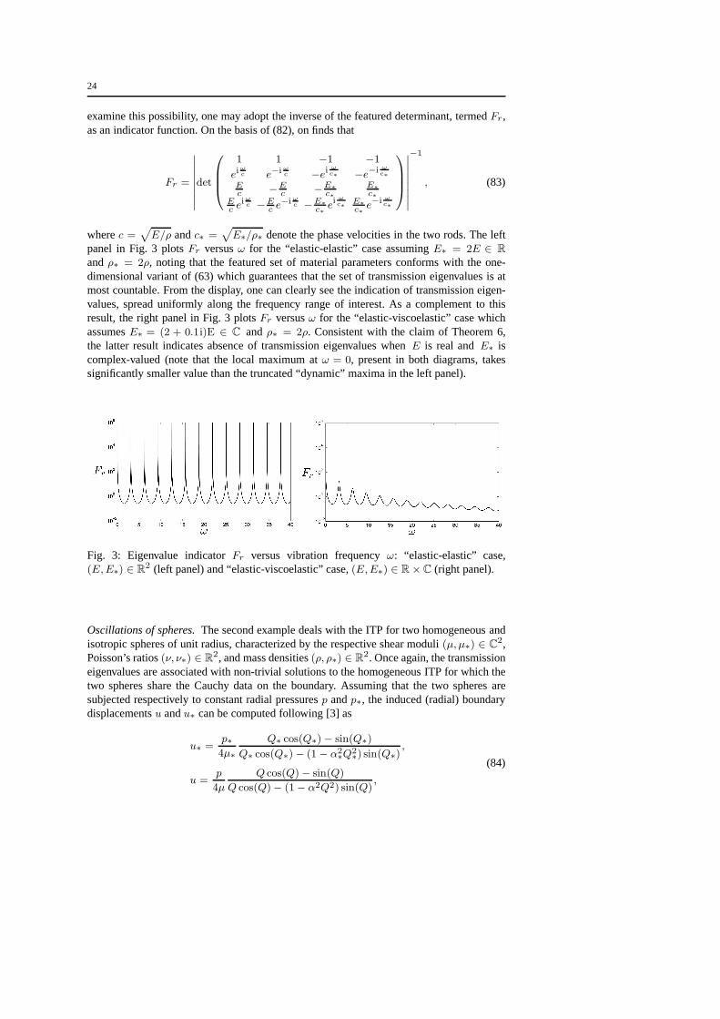
andρ∗ = 2ρ, noting that the featured set of material parameters conforms with the one-dimensional variant of (63) which guarantees that the set oftransmission eigenvalues is atmost countable. From the display, one can clearly see the indication of transmission eigen-values, spread uniformly along the frequency range of interest. As a complement to thisresult, the right panel in Fig. 3 plotsFr versusω for the “elastic-viscoelastic” case whichassumesE∗ = (2 + 0.1i)E ∈ C andρ∗ = 2ρ. Consistent with the claim of Theorem 6,the latter result indicates absence of transmission eigenvalues whenE is real andE∗ iscomplex-valued (note that the local maximum atω = 0, present in both diagrams, takessignificantly smaller value than the truncated “dynamic” maxima in the left panel).

Fig. 3: Eigenvalue indicatorFr versus vibration frequencyω: “elastic-elastic” case,(E,E∗) ∈ R

2 (left panel) and “elastic-viscoelastic” case,(E,E∗) ∈ R ×C (right panel).

Oscillations of spheres.The second example deals with the ITP for two homogeneous andisotropic spheres of unit radius, characterized by the respective shear moduli(µ, µ∗) ∈ C

2,Poisson’s ratios(ν, ν∗) ∈ R

2, and mass densities(ρ, ρ∗) ∈ R2. Once again, the transmission

eigenvalues are associated with non-trivial solutions to the homogeneous ITP for which thetwo spheres share the Cauchy data on the boundary. Assuming that the two spheres aresubjected respectively to constant radial pressuresp andp∗, the induced (radial) boundarydisplacementsu andu∗ can be computed following [3] as

u∗ =p∗4µ∗

Q∗ cos(Q∗)− sin(Q∗)

Q∗ cos(Q∗)− (1− α2∗Q

2∗) sin(Q∗)

,

u =p

4µ

Q cos(Q)− sin(Q)

Q cos(Q)− (1− α2Q2) sin(Q),

(84)

25

where

α2 =1− ν

2− 4ν, α2

∗ =1− ν∗2− 4ν∗

, Q2 =ρ ω2

4µα2 , Q2∗ =

ρ∗ω2

4µ∗α2∗. (85)

To develop an eigenvalue indicator function in the spirit ofthe previous example, one mayassume that equalityp = p∗ holds on the boundary, and define

Fs =|uu∗|

∣

∣

∣

up − u∗

p∗

∣

∣

∣

, (86)

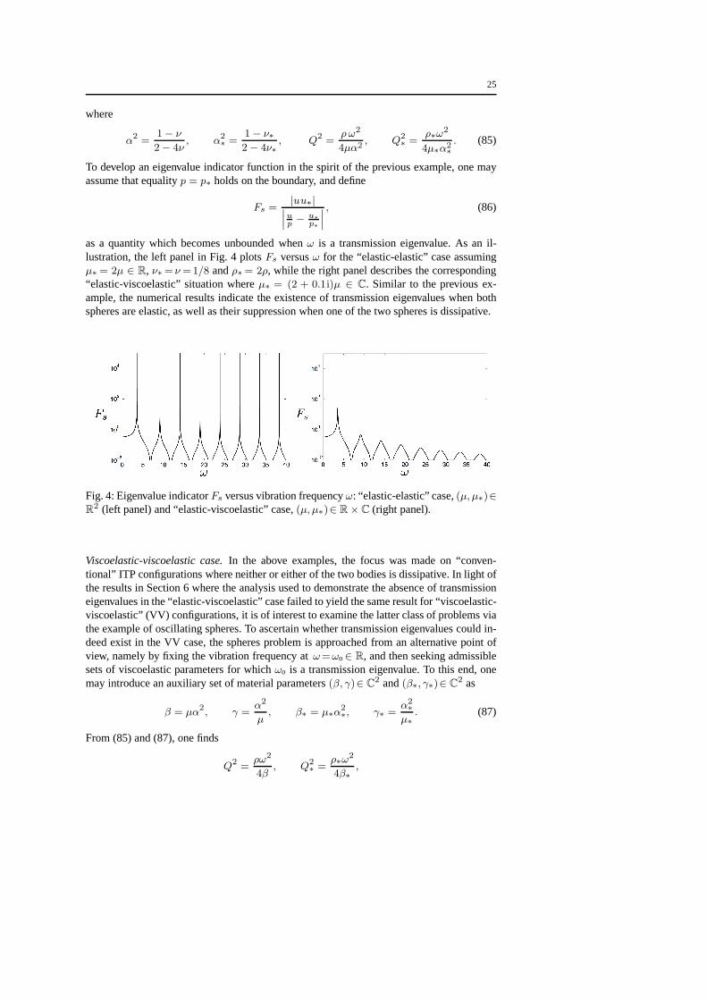
as a quantity which becomes unbounded whenω is a transmission eigenvalue. As an il-lustration, the left panel in Fig. 4 plotsFs versusω for the “elastic-elastic” case assumingµ∗ = 2µ ∈ R, ν∗= ν=1/8 andρ∗= 2ρ, while the right panel describes the corresponding“elastic-viscoelastic” situation whereµ∗ = (2 + 0.1i)µ ∈ C. Similar to the previous ex-ample, the numerical results indicate the existence of transmission eigenvalues when bothspheres are elastic, as well as their suppression when one ofthe two spheres is dissipative.

Fig. 4: Eigenvalue indicatorFs versus vibration frequencyω: “elastic-elastic” case,(µ, µ∗)∈R2 (left panel) and “elastic-viscoelastic” case,(µ, µ∗)∈ R× C (right panel).

Viscoelastic-viscoelastic case.In the above examples, the focus was made on “conven-tional” ITP configurations where neither or either of the twobodies is dissipative. In light ofthe results in Section 6 where the analysis used to demonstrate the absence of transmissioneigenvalues in the “elastic-viscoelastic” case failed to yield the same result for “viscoelastic-viscoelastic” (VV) configurations, it is of interest to examine the latter class of problems viathe example of oscillating spheres. To ascertain whether transmission eigenvalues could in-deed exist in the VV case, the spheres problem is approached from an alternative point ofview, namely by fixing the vibration frequency atω=ωo∈ R, and then seeking admissiblesets of viscoelastic parameters for whichωo is a transmission eigenvalue. To this end, onemay introduce an auxiliary set of material parameters(β, γ)∈ C

2 and(β∗, γ∗)∈ C2 as

β = µα2, γ =α2

µ, β∗ = µ∗α

2∗, γ∗ =

α2∗

µ∗. (87)

From (85) and (87), one finds

Q2 =ρω2

4β, Q2

∗ =ρ∗ω

2

4β∗,

26

which allows the boundary displacements in (84) to be rewritten as

u∗ =p∗4

(

γ∗β∗

)1

2 Q∗ cos(Q∗)− sin(Q∗)

Q∗ cos(Q∗)− [1− (β∗γ∗)1

2Q2∗] sin(Q∗)

,

u =p

4

(

γ

β

)1

2 Q cos(Q)− sin(Q)

Q cos(Q)− [1− (βγ)1

2Q2] sin(Q).

(88)

Given ωo ∈ R, (ρ, ρ∗) ∈ R2, and (β, β∗, γ∗) ∈ (C\R)3, one is now in position to seek

γ ∈ C\R such thatu = u∗ andp = p∗. On the basis of (88), the explicit solution is given by

γ =βΛ2(Q cos(Q)− sin(Q))2

[Q cos(Q)− (1 + ΛβQ2) sin(Q)]2, (89)

where

Λ =

(

γ∗β∗

)1

2 Q∗ cos(Q∗)− sin(Q∗)

Q∗ cos(Q∗)− [1− (β∗γ∗)1

2Q2∗] sin(Q∗)

. (90)

In this setting, any relevant solution in terms ofγ must also satisfy the conditions of physicaladmissibility in terms of the shear and bulk moduli

µ =

(

β

γ

)1

2

, K = 4β −4

3

(

β

γ

)1

2

,

which are subject to the ellipticity and thermomechanical stability requirements

ℜ[µ] > 0, ℑ[µ] > 0, ℜ[K] > 0, ℑ[K] > 0. (91)

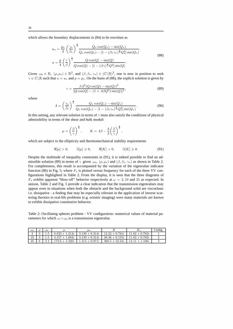
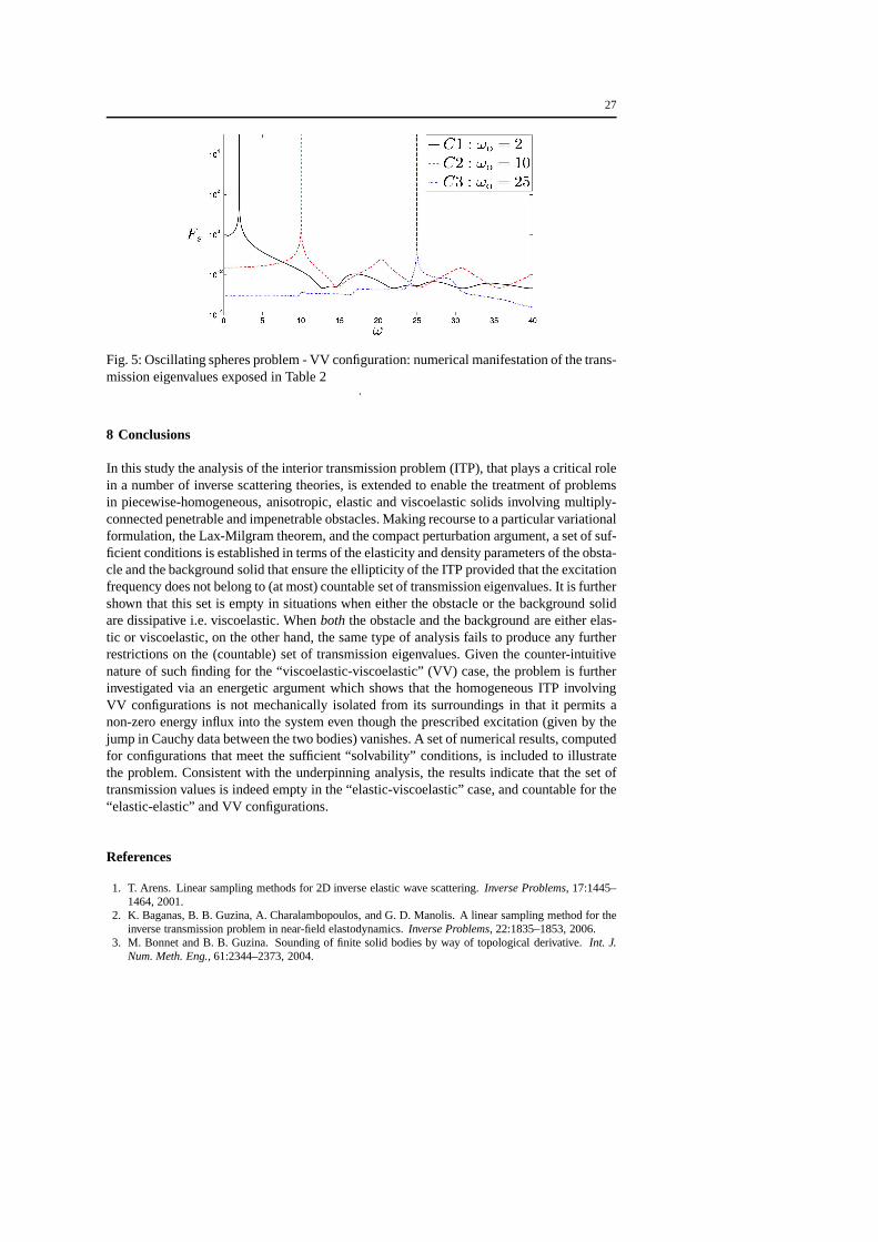
Despite the multitude of inequality constraints in (91), itis indeed possible to find an ad-missible solution (89) in terms ofγ given ωo, (ρ, ρ∗) and(β, β∗, γ∗) as shown in Table 2.For completeness, this result is accompanied by the variation of the eigenvalue indicatorfunction (86) in Fig. 5, whereFs is plotted versus frequency for each of the three VV con-figurations highlighted in Table 2. From the display, it is seen that the three diagrams ofFs exhibit apparent “blow-off” behavior respectively atω = 2, 10 and25 as expected. Inunison, Table 2 and Fig. 5 provide a clear indication that thetransmission eigenvalues mayappear even in situations when both the obstacle and the background solid are viscoelastci.e. dissipative - a finding that may be especially relevant in the application of inverse scat-tering theories to real-life problems (e.g. seismic imaging) were many materials are knownto exhibit dissipative constitutive behavior.

Table 2: Oscillating spheres problem - VV configuration: numerical values of material pa-rameters for whichω=ωo is a transmission eigenvalue.

ωo ρ ρ∗ µ µ∗ K K∗ Config.2 3 1.5 8.833 + 1.214i 3.139 + 0.314i 12.22 + 0.781i 11.82 + 0.782i 110 3 1.5 4.157 + 1.684i 3.139 + 0.314i 26.46 + 0.155i 11.82 + 0.782i 225 6 3.4 173.6 + 4.320i 1.414 + 0.071i 368.5 + 52.24i 14.11 + 1.106i 3

27

Fig. 5: Oscillating spheres problem - VV configuration: numerical manifestation of the trans-mission eigenvalues exposed in Table 2

.

8 Conclusions

In this study the analysis of the interior transmission problem (ITP), that plays a critical rolein a number of inverse scattering theories, is extended to enable the treatment of problemsin piecewise-homogeneous, anisotropic, elastic and viscoelastic solids involving multiply-connected penetrable and impenetrable obstacles. Making recourse to a particular variationalformulation, the Lax-Milgram theorem, and the compact perturbation argument, a set of suf-ficient conditions is established in terms of the elasticityand density parameters of the obsta-cle and the background solid that ensure the ellipticity of the ITP provided that the excitationfrequency does not belong to (at most) countable set of transmission eigenvalues. It is furthershown that this set is empty in situations when either the obstacle or the background solidare dissipative i.e. viscoelastic. Whenboth the obstacle and the background are either elas-tic or viscoelastic, on the other hand, the same type of analysis fails to produce any furtherrestrictions on the (countable) set of transmission eigenvalues. Given the counter-intuitivenature of such finding for the “viscoelastic-viscoelastic”(VV) case, the problem is furtherinvestigated via an energetic argument which shows that thehomogeneous ITP involvingVV configurations is not mechanically isolated from its surroundings in that it permits anon-zero energy influx into the system even though the prescribed excitation (given by thejump in Cauchy data between the two bodies) vanishes. A set ofnumerical results, computedfor configurations that meet the sufficient “solvability” conditions, is included to illustratethe problem. Consistent with the underpinning analysis, the results indicate that the set oftransmission values is indeed empty in the “elastic-viscoelastic” case, and countable for the“elastic-elastic” and VV configurations.

References

1. T. Arens. Linear sampling methods for 2D inverse elastic wave scattering.Inverse Problems, 17:1445–1464, 2001.

2. K. Baganas, B. B. Guzina, A. Charalambopoulos, and G. D. Manolis. A linear sampling method for theinverse transmission problem in near-field elastodynamics. Inverse Problems, 22:1835–1853, 2006.

3. M. Bonnet and B. B. Guzina. Sounding of finite solid bodies by way of topological derivative.Int. J.Num. Meth. Eng., 61:2344–2373, 2004.

28

4. A. J. Burton and G. F. Miller. The application of the integral equation methods to the numerical solutionof some exterior boundary-value problems.Proc. Roy. Soc. Lond. A, 323:201–210, 1971.

5. F. Cakoni and D. Colton.Qualitative methods in inverse scattering theory. Springer-Verlag, Berlin,2006.

6. F. Cakoni, D. Colton, and H. Haddar. The linear sampling method for anisotropic media.J. Comput.Appl. Math., 146:285–299, 2002.

7. F. Cakoni and H. Haddar. The linear sampling method for anisotropic media: Part 2. Preprints 26, MSRIBerkeley, California, 2001.

8. F. Cakoni and H. Haddar. A variational approach for the solution of the electromagnetic interior trans-mission problem for anisotropic media.Inverse Problems and Imaging, 1:443–456, 2007.

9. J. M. Carcione and F. Cavallini. Energy balance and fundamental relations in anisotropic-viscoelasticmedia.Wave motion, 18:11–20, 1993.

10. A. Charalambopoulos. On the interior transmission problem in nondissipative, inhomogeneous,anisotropic elasticity.J. Elasticity, 67:149–170, 2002.

11. A. Charalambopoulos and K. A. Anagnostopoulos. On the spectrum of the interior transmission problemin isotropic elasticity.J. Elasticity, 90:295313, 2008.

12. A. Charalambopoulos, D. Gintides, and K. Kiriaki. The linear sampling method for the transmissionproblem in three-dimensional linear elasticity.Inverse Problems, 18:547558, 2002.

13. A. Charalambopoulos, A. Kirsch, K. A. Anagnostopoulos,D. Gintides, and K. Kiriaki. The factorizationmethod in inverse elastic scattering from penetrable bodies. Inverse Problems, 23:27–51, 2007.

14. D. Colton, J. Coyle, and P. Monk. Recent developments in inverse acoustic scattering theory.SIAMReview, 42:369–414, 2000.

15. D. Colton and A. Kirsch. A simple method for solving inverse scattering problems in the resonanceregion. Inverse Problems, 12:383–393, 1996.

16. D. Colton, A. Kirsch, and L. Paivarinta. Far-field patterns for acoustic waves in an inhomogeneousmedium.SIAM J. Math. Anal., 20:1472–1483, 1989.

17. D. Colton and R. Kress.Inverse acoustic and electromagnetic scattering theory. Springer, 1998.18. D. Colton and R. Kress. Using fundamental solutions in inverse scattering.Inverse Problems, 22:R49–

R66, 2006.19. D. Colton, L. Paivarinta, and J. Sylvester. The interiortransmission problem.Inverse Problems and

Imaging, 1:13–28, 2007.20. W. N. Findley, J. S. Lai, and K. Onaran.Creep and Relaxation of Nonlinear Viscoelastic Materials.

Dover, New York, 1989.21. W. Flugge.Viscoelasticity. Springer-Verlag, 1975.22. B. B. Guzina and A. I. Madyarov. A linear sampling approach to inverse elastic scattering in piecewise-

homogeneous domains.Inverse Problems, 23:1467–1493, 2007.23. H. Haddar. The interior transmission problem for anisotropic maxwells equations and its applications to

the inverse problem.Math. Meth. Appl. Sci., 27:2111–2129, 2004.24. P. Hahner. On the uniqueness of the shape of a penetrable, anisotropic obstacle.J. Comput. Appl. Math.,

116:167–180, 2000.25. A. Kirsch. An integral equation approach and the interior transmission problem for maxwell’s equations.

Inverse Problems and Imaging, 1:107–127, 2007.26. A. Kirsch. On the existence of transmission eigenvalues. Inverse Problems and Imaging, 3:155–172,

2009.27. A. Kirsch and N. Grinberg.The Factorization Method for Inverse Problems. Oxford University Press,

New York, 2008.28. J. K. Knowles. On the representation of the elasticity tensor for isotropic media.J. Elasticity, 39:175–

180, 1995.29. V. D. Kupradze.Potential methods in the theory of elasticity. Israel Program for Scientific Translations,

1965.30. Y. Liu and F. J. Rizzo. Hypersingular boundary integral equations for radiation and scattering of elastic

waves in three dimensions.Comp. Meth. Appl. Mech. Eng., 107:131–144, 1993.31. A. I. Madyarov and B. B. Guzina. A radiation condition forlayered elastic media.J. Elasticity, 82:73–98,

2006.32. L. E. Malvern.Introduction to the Mechanics of a Continuous Medium. Prentice-Hall, Englewood Cliffs,

1969.33. J. E. Marsden and T. J. R. Hughes.Mathematical foundations of elasticity. Dover, 1994.34. G Mataraezo. Irreversibility of time and symmetry property of relaxation function in linear viscoelastic-

ity. Mechanics Research Communications, 28:373–380, 2001.35. W. McLean. Strongly elliptic systems and boundary integral equations. Cambridge university press,

2000.

29

36. M. M. Mehrabadi, S. C. Cowin, and C. O. Horgan. Strain energy density bounds for linear anisotropicelastic materials.J. Elasticity, 30:191–196, 1993.

37. J. Necas and I. Hlavacek.Mathematical theory of elastic and elasto-plastic bodies:an introduction.Elsevier, 1981.

38. S. Nintcheu Fata and B. B. Guzina. Elastic scatterer reconstruction via the adjoint sampling method.SIAM J. Appl. Math, 67:1330–1352, 2004.

39. S. Nintcheu Fata and B. B. Guzina. A linear sampling method for near-field inverse problems in elasto-dynamics.Inverse problems, 20:713–736, 2004.

40. L. Paivarinta and J. Sylvester. Transmission eigenvalues. SIAM J. Math. Anal., 40:738–753, 2008.41. R. Potthast. A survey on sampling and probe methods for inverse problems.Inverse Problems, 22:R1–47,

2006.42. T Pritz. The poisson’s loss factor of solid viscoelasticmaterials. Journal of Sound and Vibration,

306:790–802, 2007.43. L. Pyl, D. Clouteau, and G. Degrande. A weakly singular boundary integral equation in elastodynamics

for heterogeneous domains mitigating fictitious eigenfrequencies. Eng. Anal. Bound. Elem., 28:1493–1513, 2004.

44. B. P. Rynne and Sleeman B. D. The interior transmission problem and inverse scattering from inhomo-geneous media.SIAM J. Math. Anal., 22:1755–1762, 1991.

45. I. M. Shter. Generalization of onsager’s principle and its application.Journal of Engineering Physicsand Thermophysics, 25:1319–1323, 1973.

46. J. Wloka.Partial differential equations. Cambridge University Press, 1992.47. K. Yosida.Functional Analysis. Springer-Verlag, Berlin, 1980.