ON THE ERROR ESTIMATES FOR THE ROTATIONAL PRESSURE-CORRECTION … · 2018-11-16 · MATHEMATICS OF COMPUTATION Volume 73, Number 248, Pages 1719{1737 S 0025-5718(03)01621-1 Article

MATHEMATICS OF COMPUTATIONVolume 73, Number 248, Pages 1719–1737S 0025-5718(03)01621-1Article electronically published on December 19, 2003

ON THE ERROR ESTIMATESFOR THE ROTATIONAL PRESSURE-CORRECTION

PROJECTION METHODS

J. L. GUERMOND AND JIE SHEN

Abstract. In this paper we study the rotational form of the pressure-correc-tion method that was proposed by Timmermans, Minev, and Van De Vosse.We show that the rotational form of the algorithm provides better accuracy interms of the H1-norm of the velocity and of the L2-norm of the pressure thanthe standard form.

1. Introduction

There are numerous way to discretize the unsteady incompressible Navier-Stokesequations in time. Undoubtedly, the most popular one consists of using projectionmethods. This class of techniques has been introduced by Chorin and Temam[2, 3, 17]. They are time marching algorithms based on a fractional step techniquethat may be viewed as a predictor-corrector strategy aiming at uncoupling viscousdiffusion and incompressibility effects. The method proposed originally, althoughsimple, is not satisfactory since its convergence rate is irreducibly limited to O(δt).This limitation comes from the fact that the method is basically an artificial com-pressibility technique as shown in [11] and [13]. To cure these problems, numerousmodifications have been proposed, among which are pressure-correction methods(see [6, 20]) and splitting techniques based on extrapolated pressure boundary con-ditions (see [10, 9]).

Pressure-correction methods are widely used and have been extensively ana-lyzed. These schemes are composed of two substeps by time step: the pressure ismade explicit in the first substep and is corrected in the second one by projectingthe provisional velocity onto the space of incompressible vector fields. Rigoroussecond-order error estimates for the velocity have been proved by E and Liu [4] andShen [15] in the semi-discrete case and by Guermond [7] and E and Liu [5] in thefully discrete case. We refer also to [16] and [1] for different proofs based on normalmode analysis in the half plane and in a periodic channel, respectively.

It is well known that standard pressure-correction schemes still suffer from thenonphysical pressure boundary condition which induces a numerical boundary layer

Received by the editor February 11, 2002 and, in revised form, March 2, 2003.2000 Mathematics Subject Classification. Primary 65M12, 35Q30, 76D05.Key words and phrases. Navier-Stokes equations, projection methods, fractional step methods,

incompressibility, finite elements, spectral approximations.The work of the second author is partially supported by NFS grants DMS-0074283 and DMS-

0311915. Part of the work was completed while this author was a CNRS “Poste Rouge” visitorat LIMSI.

c©2003 American Mathematical Society

1719

License or copyright restrictions may apply to redistribution; see https://www.ams.org/journal-terms-of-use

1720 J. L. GUERMOND AND JIE SHEN

and, consequently, degrades the accuracy of the pressure approximation. In 1996,Timmermans, Minev and Van De Vosse [19] proposed a modified version of thepressure-correction scheme, which we shall hereafter refer to as the rotational formof the pressure-correction scheme for reasons we shall specify later, and they showednumerically that it leads to improved pressure approximation. Recently, Brown,Cortez and Minion [1] used normal mode analysis to study the accuracy of thisscheme in a periodic channel and showed that the pressure approximation in thisparticular case is second-order accurate. However, whether the rotational form canyield second-order pressure approximation in more general domains is still an openquestion. In fact, to the best of the authors’ knowledge, there is no rigorous analysisavailable yet in the literature for this type of algorithms in general domains.

The aim of this paper is to provide a rigorous stability and error analysis forthe rotational form of pressure-correction schemes. Our results indicate that whilethe rotational form of pressure-correction schemes does not improve the accuracyon the approximate velocity in the L2-norm, it does improve the accuracy on thisquantity in the H1-norm and that on the approximate pressure in the L2-norm fromfirst-order to 3

2 -order. Based on our numerical results, this 32 -order convergence rate

on the pressure appears to be the best possible for the rotational form of pressure-correction schemes in general domains.

This paper is organized as follows. In §2, we introduce notation and recallimportant results that are used repeatedly in the core of the paper. In §3, wepresent the rotational form of the pressure-correction algorithm using a second-order backward difference formula (BDF2) to march in time. In this section, wealso analyze a singular perturbation of the Navier-Stokes equations that mimics thecharacteristics of the new scheme. The analysis of the discrete scheme is performedin §4. We illustrate the performance of the proposed scheme in §5 by showingnumerical convergence tests using P2/P1 finite elements and PN/PN−2 spectralapproximations.

2. Notation and preliminaries

We now introduce some notation. We shall consider the time-dependent Navier-Stokes equations on a finite time interval [0, T ] and in an open, connected, andbounded domain Ω ⊂ Rd (d = 2 or 3) with a boundary Γ sufficiently smooth. Letδt > 0 be a time step and set tk = kδt for 0 ≤ k ≤ K = [T/δt].

Let φ0, φ1, . . . , φK be some sequence of functions in some Hilbert space E. Wedenote by φδt this sequence, and we use the following discrete norms:

(2.1) ‖φδt‖l2(E) :=

(δt

K∑k=0

‖φk‖2E

)1/2

, ‖φδt‖l∞(E) := max0≤k≤K

(‖φk‖E

).

We use the standard Sobolev spaces Hm(Ω) (m = 0,±1, · · · ) whose norms aredenoted by ‖ ·‖m. In particular, the norm and inner product of L2(Ω) = H0(Ω) aredenoted by ‖ · ‖ and (·, ·), respectively. We also set L2

0(Ω) = q ∈ L2(Ω) :∫

Ω qdx =0. To account for homogeneous Dirichlet boundary conditions, we define H1

0 (Ω) =v ∈ H1(Ω) : v|Γ = 0. Thanks to the Poincare inequality, for v ∈ H1

0 (Ω)d, ‖∇v‖is a norm equivalent to ‖v‖1. We also have

(2.2) ‖∇v‖2 = ‖∇·v‖2 + ‖∇×v‖2, ∀v ∈ H10 (Ω)d.


ROTATIONAL PRESSURE-CORRECTION METHOD 1721

We introduce two spaces of incompressible vector fields

H = v ∈ L2(Ω)d; ∇·v = 0; v · n|Γ = 0,(2.3)

V = v ∈ H1(Ω)d; ∇·v = 0; v|Γ = 0,(2.4)

and we define PH as the L2-orthogonal projector in H , i.e.,

(2.5) (u− PHu, v) = 0 ∀u ∈ L2(Ω)d, v ∈ H.We denote by c a generic constant that is independent of ε and δt but possibly

depends on the data and the solution. We shall use the expression A . B to saythat there exists a generic constant c such that A ≤ cB.

Next, we define the inverse Stokes operator S : H−1(Ω)d −→ V . For all v inH−1(Ω)d, (S(v), r) ∈ V × L2

0(Ω) is the solution to the following problem(∇S(v),∇w) − (r,∇·w) = 〈v, w〉, ∀w ∈ H1

0 (Ω)d,(q,∇·S(v)) = 0, ∀q ∈ L2

0(Ω),

where 〈·, ·〉 denotes the duality paring between H−1(Ω)d and H10 (Ω)d.

We assume that Γ is sufficiently smooth so that the following regularity propertieshold (cf. [18]):

(2.6) ∀v ∈ L2(Ω)d, ‖S(v)‖2 + ‖∇r‖ ≤ c‖v‖.The following properties of S are proved in [8].

Lemma 2.1. For all v in H10 (Ω)d and all 0 < γ < 1 we have

(∇S(v),∇v) ≥ (1− γ)‖v‖2 − c(γ)‖v − v?‖2, ∀v? ∈ H.In particular,

(∇S(v),∇v) = ‖v‖2, ∀v ∈ V.

Lemma 2.2. The bilinear form H−1(Ω)d × H−1(Ω)d 3 (v, w) 7−→ 〈S(v), w〉 ∈ Rinduces a semi-norm on H−1(Ω)d that we denote by | · |?, and

|v|? = ‖S(v)‖1 ≤ c‖v‖−1, ∀v ∈ H−1(Ω)d.

3. Rotational form of the pressure-correction methods

We consider the movement of an incompressible fluid inside Ω whose velocity uand pressure p are governed by the Navier-Stokes equations:

(3.1)

∂tu− ν∇2u+ u·∇u+∇p = f in Ω× [0, T ],

∇·u = 0 in Ω× [0, T ],u|Γ = 0, u|t=0 = u0 in Ω.

The boundary condition on the velocity is set to zero for the sake of simplicity, andu0 ∈ H is an initial velocity field.

Since for projection methods the treatment of the nonlinear term does not con-tribute in any essential way to the error behaviors, we shall describe the rotationalpressure-correction scheme and carry out all the error analyses for the linearizedequations only, thus avoiding technicalities associated with the nonlinearities whichobscure the essential difficulties. In fact, the error estimates established here forthe linearized equations are valid for the fully nonlinear Navier-Stokes equations,provided the solution is sufficiently smooth, and these estimates can be proved bycombining the techniques used here and those in [7, 15, 17]. In practice, the nonlin-ear terms can be treated either implicitly, semi-implicitly or explicitly depending on



various factors such as stability, simplicity, efficiency, and the practitioners’ pref-erences. Thus, to fix the ideas, we will only consider the approximation of thefollowing linearized Navier-Stokes equations (we set ν = 1 for simplicity):

(3.2)

∂tu−∇2u+∇p = f in Ω× [0, T ],

∇·u = 0 in Ω× [0, T ],u|Γ = 0, u|t=0 = u0 in Ω.

To simplify our presentation, we assume that the unique solution (u, p) to the abovesystem is sufficiently smooth in time and in space.

3.1. Description of the scheme. Before introducing the rotational form of thepressure-correction algorithm, let us recall its standard form using BDF2 to marchin time. Using the linearized version of the Navier-Stokes equations, the first sub-step accounting for viscous diffusion is

(3.3)

3uk+1 − 4uk + uk−1

2δt−∇2uk+1 +∇pk = f(tk+1),

uk+1|Γ = 0,

and the second substep accounting for incompressibility is

(3.4)

3uk+1 − 3uk+1

2δt+∇(pk+1 − pk) = 0,

∇·uk+1 = 0,uk+1 · n|Γ = 0.

This step is usually referred to as the projection step, for it is a realization of theidentity uk+1 = PH u

k+1.This scheme has been thoroughly studied (cf. [12, 4, 15, 7]). Though it is

second-order accurate on the velocity in the L2-norm, it is plagued by a numericalboundary layer that prevents it from being fully second-order on the H1-norm ofthe velocity and on the L2-norm of the pressure. Actually, from (3.4) we observethat ∇(pk+1 − pk) · n|Γ = 0 which implies that

(3.5) ∇pk+1 · n|Γ = ∇pk · n|Γ = · · ·∇p0 · n|Γ.

It is this nonrealistic Neumann boundary condition on the pressure that introducesthe numerical boundary layer referred to above and consequently limits the accuracyof the scheme.

In 1996, a modified scheme with a divergence correction has been proposed in[19]. More precisely, the second step (3.4) is replaced by

(3.6)

3uk+1 − 3uk+1

2δt+∇(pk+1 − pk +∇·uk+1) = 0,

∇·uk+1 = 0,uk+1 · n|Γ = 0.

The authors have shown numerically that the modified scheme (3.3)–(3.6) providessignificantly better approximations for the pressure. To the best of our knowledge,no rigorous analysis for the modified scheme (3.3)–(3.6) has yet been proposed inthe literature.



To understand why the modified scheme performs better, we take the sum of(3.3) and (3.6) (note from (3.6) that ∇×∇×uk+1 = ∇×∇×uk+1), and we get

(3.7)

3uk+1 − 4uk + uk−1

2δt+∇×∇×uk+1 +∇pk+1 = f(tk+1),

∇·uk+1 = 0,

with uk+1 · n|Γ = 0. We observe from (3.7) that

∂pk+1

∂n|Γ = (f(tk+1)−∇×∇×uk+1) · n|Γ,

which, unlike (3.5), is a consistent pressure boundary condition. The splitting errornow manifests itself only in the form of an inexact tangential boundary conditionfor the velocity.

In view of (3.7), where the operator∇×∇×plays a key role, we shall hereafter referto the algorithm (3.3)–(3.6) as the pressure-correction scheme in rotational form,and we shall refer to the original algorithm (3.3)–(3.4) as the pressure-correctionscheme in standard form.

The aim of this paper is to prove stability and derive error estimates for thescheme (3.3)–(3.6).

3.2. Initialization of the scheme. Note that we need (u0, u0, p0) and (u1, u1, p1)to start the scheme (3.3)–(3.6). We set

(3.8) u0 = u0, u0 = u0, p

0 = p(0),

where p(0) is determined from u0 and equations (3.2). We solve (u1, u1, p1) fromthe following first-order pressure-correction projection scheme:

(3.9)

u1 − u0

δt−∇2u1 +∇p0 = f(t1),

u1|Γ = 0

and

(3.10)

u1 − u1

δt+∇(p1 − p0) = 0,

∇·u1 = 0,u1 · n|Γ = 0.

Let us denote R1 = ut(δt) − u(δt)−u(0)δt . The error equation corresponding to (3.9)

is(u(δt)− u1)− δt∆(u(δt)− u1) = −δt∇(p(δt)− p(0))− δtR1 = O(δt2),

(u(δt)− u1)|∂Ω = 0.(3.11)

One derives immediately from the standard PDE theory that

(3.12) ‖u(δt)− u1‖+ δt12 ‖∇(u(δt)− u1)‖+ δt‖∆(u(δt)− u1)‖ . δt2.

The error equation corresponding to (3.10) is

(3.13) ∇(p(δt)− p1) = − (u(δt)− u1)− (u(δt)− u1)δt

+∇(p(δt)− p(0)).

We derive easily from (3.13) and (3.12) that

(3.14) ‖∇(p(δt)− p1)‖ . δt.



Repeating the same above procedure for (3.3)–(3.6) with k = 1, we obtain

(3.15) ‖u(2δt)− u2‖+ δt12 ‖∇(u(2δt)− u2)‖ + δt‖∆(u(2δt)− u2)‖ . δt2.

(3.16) ‖∇(p(2δt)− p2)‖ . δt.

3.3. Time continuous version: a singularly perturbed PDE. Since the essen-tial error behaviors of (3.3)–(3.6) are determined by its limiting system as δt −→ 0,it is instructive to study the following singularly perturbed system, which is ob-tained by eliminating uk from (3.3)–(3.6) and by dropping some lower-order termsas ε ∼ δt→ 0:

∂tuε −∇2uε +∇pε = f, uε|Γ = 0,(3.17)

∇·uε − ε∇2φε = 0, ∂φε

∂n |Γ = 0,(3.18)ε∂tp

ε = φε −∇·uε,(3.19)

with uε|t=0 = u(0) and pε(0) = p(0).The following lemma exhibits the essential feature of this singularly perturbed

system and is the key to prove higher order estimates.

Lemma 3.1. Provided that u and p are smooth enough in time and space, we have

‖∇·uε‖L∞(L2(Ω)) . ε32 .

Proof. We shall first derive some a priori estimates.We denote e = uε − u and q = pε − p. Subtracting (3.17) from (3.2), we find

et −∇2e+∇q = 0, e|Γ = 0,(3.20)

∇·e− ε∇2φε = 0, ∂φε

∂n |Γ = 0,(3.21)εqt = φε −∇·uε − εpt,(3.22)

with e(0) = 0 and q(0) = 0.Taking the inner product of the time derivative of (3.20) with et, we find

(3.23)12∂t‖et‖2 + ‖∇et‖2 − (qt,∇·et) = 0.

Using (3.21) and (3.22),

−(qt,∇·et) = −ε(qt,∆φεt ) = −(φε − ε∆φε − εpt,∆φεt )

=12∂t‖∇φε‖2 +

ε

2∂t‖∆φε‖2 − ε(∇pt,∇φεt )

=12∂t‖∇φε‖2 +

ε

2∂t‖∆φε‖2 − ε∂t(∇pt,∇φε) + ε(∇ptt,∇φε).

(3.24)

The above two relations lead to12∂t‖et‖2 + ‖∇et‖2 +

12∂t‖∇φε‖2 +

ε

2∂t‖∆φε‖2

= ε∂t(∇pt,∇φε)− ε(∇ptt,∇φε),(3.25)

since we have e(0) = 0 and q(0) = 0, which imply that φε(0) = 0 and et(0) = 0.Therefore, an application of the Gronwall lemma to the above relation leads to

(3.26) ‖et(t)‖2 + ‖∇φε(t)‖2 + ε‖∆φε(t)‖2 +∫ t

0

‖∇et(s)‖2ds . ε2.



We immediately obtain

(3.27) ‖∇·uε(t)‖2 = ε2‖∆φε(t)‖2 . ε3.

Lemma 3.2. Provided that u and p are smooth enough in time and space, we have

‖u− uε‖L2(L2(Ω)d) . ε2.

Proof. We take the inner product of (3.20) with S(e), where S is the inverse Stokesoperator defined in §2. Since S(e) ∈ V , we find

(3.28)12∂t|e|2? + (∇e,∇S(e)) = 0.

Thanks to Lemma 2.1, we have

(3.29)12∂t|e|2? +

12‖e‖2 . ‖e− PHe‖2.

By the definition of PH , we can write e−PHe = ∇r with ∂r∂n |∂Ω = 0. Consequently

∇·e = ∆r and from (3.21), we infer r = εφε and

(3.30) ‖e− PHe‖2 = ‖∇r‖2 = ε2‖∇φε‖2.

Applying the Gronwall lemma to (3.29) and taking into account (3.26), we derive

|e(t)|2? +∫ t

0

‖e(s)‖2ds . ε2

∫ t

0

‖∇φε(s)‖2ds . ε4.

Remark 3.1. These two lemmas are essential to understanding the arguments thatwill be used in the discrete case. They will have two discrete counterparts in theform of Lemmas 4.1 and 4.2.

4. Error estimates for the time discrete case

Let us first introduce some notation. For any sequence φ0, φ1, . . ., we set

δtφk = φk − φk−1, δttφ

k = δt(δtφk), δtttφk = δt(δttφk)

and

(4.1)ek = u(tk)− uk, ek = u(tk)− uk,ψk = p(tk+1)− pk, qk = p(tk)− pk.

The main result in this paper is

Theorem 4.1. Provided the solution to (3.2) is smooth enough in time and space,the solution (uk, uk, pk) to (3.3)–(3.6) satisfies the estimates

‖eδt‖l2(L2(Ω)d) + ‖eδt‖l2(L2(Ω)d) . δt2,‖eδt‖l2(H1(Ω)d) + ‖eδt‖l2(H1(Ω)d) + ‖qδt‖l2(L2(Ω)) . δt

32 .

The remainder of this section is devoted to the proof of the above theorem. Theproof of Theorem 4.1 will be carried out through a sequence of estimates presentedbelow.



4.1. Stability and a priori estimate on ‖∇· uk‖. We first establish a resultsimilar to that of Lemma 3.1.

Lemma 4.1. Under the hypotheses of Theorem 4.1, we have

‖∇·uδt‖l∞(L2(Ω)) . δt3/2,‖eδt − eδt‖`2(L2(Ω)d) . δt2,

‖δteδt − δteδt‖l2(L2(Ω)d) . δt5/2.

Proof. The proof of this lemma follows the same principle as that we used in §3for the time continuous version of the algorithm. The critical step here consists inworking with the time increments δtek+1 and δte

k+1, which corresponds to takingthe inner product of the time derivative of (3.20) with ∂te.

Let us first write the equations that control the time increments of the errors.We define

(4.2) Rk =3u(tk)− 4u(tk−1) + u(tk−2)

2δt− ∂tu(tk).

Then, for k ≥ 1, we have

(4.3)

3δtek+1 − 4δtek + δte

k−1

2δt−∆δtek+1 +∇δtψk = δtR

k+1,

δtek+1|Γ = 0

and

(4.4)

3

2δtδte

k+1 +∇(δtqk+1 +∇·ek+1) = 32δt

δtek+1 +∇(δtψk +∇·ek),

δtek+1 · n|Γ = 0.

We take the inner product of (4.3) with 4δt δtek+1 to get

2(δtek+1, 3δtek+1 − 4δtek + δtek−1) + 4δt‖∇δtek+1‖2 + 4δt(δtek+1,∇δtψk)(4.5)

= 4δt(δtek+1, δtRk+1) ≤ 2δt‖δtek+1‖2 + 2δt‖δtRk+1‖2.

The treatment of the first term is quite technical but similar to that in [8]. For thereaders’ convenience, we show the details below. We denote

I =2(δtek+1, 3δtek+1 − 4δtek + δtek−1)

=6(δtek+1, δtek+1 − δtek+1) + 2(δtek+1 − δtek+1, 3δtek+1 − 4δtek + δte

k−1)

+2(δtek+1, 3δtek+1 − 4δtek + δtek−1),

and we denote by I1, I2 and I3 the three terms in the right-hand side. Using thealgebraic identities

2(ak+1, ak+1 − ak) = |ak+1|2 + |ak+1 − ak|2 − |ak|2,(4.6)

2(ak+1, 3ak+1 − 4ak + ak−1) = |ak+1|2 + |2ak+1 − ak|2 + |δttak+1|2(4.7)

−|ak|2 − |2ak − ak−1|2,we derive

I1 = 3‖δtek+1‖2 + 3‖δtek+1 − δtek+1‖2 − 3‖δtek+1‖2,I3 = ‖δtek+1‖2 + ‖2δtek+1 − δtek‖2 + ‖δtttek+1‖2 − ‖δtek‖2 − ‖2δtek − δtek−1‖2.



Due to (4.4) and using the fact that ek ∈ H , we derive the equality

3

2δtI2 = 2(∇δt(qk+1 − ψk) +∇∇·δtek+1, 3δtek+1 − 4δtek + δte

k−1) = 0.

Combining all the above results, we obtain

3‖δtek+1‖2− 3‖δtek+1‖2 + 3‖δtek+1 − δtek+1‖2 + ‖δtek+1‖2(4.8)

+ ‖2δtek+1 − δtek‖2 − ‖δtek‖2 − ‖2δtek − δtek−1‖2 + ‖δtttek+1‖2

+ 4δt‖∇δtek+1‖2 + 4δt(δtek+1,∇δtψk) = 4δt(δtek+1, δtRk+1).

By taking the square of (4.4), multiplying the result by 43δt

2 and integrating overthe domain, we have

3‖δtek+1‖2+4δt2

3‖∇(δtqk+1 +∇·ek+1)‖2 = 3‖δtek+1‖2(4.9)

+4δt(δtek+1,∇(δtψk +∇·ek)) +4δt2

3‖∇(δtψk +∇·ek)‖2.

The last two terms in the above relation can be bounded as follows.The term 4δt(δtek+1,∇δtψk) cancels out with the same term in (4.8). Integrating

by parts and using (4.6), we infer

4δt(δtek+1,∇∇·ek) = −4δt(∇·(ek+1 − ek),∇·ek)

= 2δt(‖∇·ek‖2 − ‖∇·ek+1‖2 + ‖∇·δtek+1‖2).(4.10)

The term 2δt‖∇·δtek+1‖2 can be controlled by 4δt‖∇δtek+1‖2 in (4.8), thanks tothe identity (2.2), we have

(4.11) ‖∇δtek+1‖2 = ‖∇× δtek+1‖2 + ‖∇·δtek+1‖2.

For ‖∇(δtψk +∇·ek)‖2, we have

‖∇(δtψk +∇·ek)‖2 =‖∇(δtqk +∇·ek) +∇δttp(tk+1)‖2

≤(cδt2 + ‖∇(δtqk +∇·ek)‖

)2≤c δt4 + 2cδt2‖∇(δtqk +∇·ek)‖+ ‖∇(δtqk +∇·ek)‖2

≤c δt4 + cδt(δt2 + ‖∇(δtqk +∇·ek)‖2) + ‖∇(δtqk +∇·ek)‖2

≤c δt3 + (1 + cδt)‖∇(δtqk +∇·ek)‖2.

(4.12)

Combining the relations (4.8)–(4.12), we derive

3‖δt(ek+1 − ek+1)‖2 + ‖δtek+1‖2 + ‖2δtek+1 − δtek‖2 + ‖δtttek+1‖2

+ 2δt‖∇δtek+1‖2 + 2δt‖∇·ek+1‖2 +43δt2‖∇(δtqk+1 +∇·ek+1)‖2

≤ cδt5 + 2δt‖δtek+1‖2 + (1 + cδt)43δt2‖∇(δtqk +∇·ek)‖2

+ ‖δtek‖2 + ‖2δtek − δtek−1‖2 + 2δt‖∇·ek‖2 + 2δt‖δtRk+1‖2.



Finally, applying the discrete Gronwall lemma to the above relation and taking intoaccount the initial estimates (3.12)–(3.16), we obtain

δt‖∇·ek+1‖2 + ‖δtek+1‖2 + ‖2δtek+1 − δtek‖2 +k∑l=2

‖δtel+1 − δtel+1‖2

+ δtk∑l=2

‖∇δtel+1‖2 + δt2‖∇(δtqk+1 +∇·ek+1)‖2

≤ c(δt4 + δt‖∇·e2‖2 + ‖δte2‖2 + ‖2δte2 − δte1‖2 + δt2‖∇(δtq2 +∇·e2)‖2

)+ c δt

k∑l=2

‖δtRl+1‖2

≤ c δt4 + δt

k∑l=2

‖δtRl+1‖2 . δt4.

(4.13)

The estimates on ∇·uδt and δteδt − δteδt are now direct consequences of the aboveinequality. To derive the estimate on eδt − eδt, we use (3.6) to infer

ek+1 − ek+1 = −2δt3∇(δtqk+1 +∇·ek+1 − δtp(tk+1)).

Then, it is clear that

‖eδt − eδt‖`2(L2(Ω)d) . δt‖∇(δtqδt +∇·eδt)‖`2(L2(Ω)d) + δt2 . δt2.

Remark 4.1. From (4.13), we observe the remarkable fact that the bound‖∇·uδt‖l2(L2(Ω)) ≤ δt3/2 still holds even if we replace the second-order BDF2 timestepping in (3.3) and (3.6) by the first-order backward Euler time stepping (i.e., inthe case Rk+1 ∼ O(δt)).

4.2. Error estimates. We start with a result similar to that stated in Lemma 3.2.


‖eδt‖l2(L2(Ω)d) . δt2.

Proof. From (3.6), we can write

(4.14) uk+1 = uk+1 − 2δt3∇(pk+1 − pk +∇·uk+1).

Substituting the above relation in (3.3) and considering the error equation, weobtain

(4.15)3ek+1 − 4ek + ek−1

2δt−∇2ek+1 +∇γk+1 = Rk+1,

where ∇γk+1 represents all the gradient terms in the error equation and Rk+1 isdefined in (4.2).

As in the time continuous case, we make use of the inverse Stokes operator. Bytaking the inner product of (4.15) with 4δtS(ek+1) and using the identity (4.7), we



obtain

|ek+1|2? + |2ek+1 − ek|2?+|δttek+1|2? + 4δt(∇S(ek+1),∇ek+1)

= 4δt(Rk+1, S(ek+1)) + |ek|2? + |2ek − ek−1|2?.

Thanks to Lemma 2.1 and the fact that ek+1 is in H , we deduce

4δt(∇S(ek+1),∇ek+1) ≥ 2δt‖ek+1‖2 − cδt‖ek+1 − ek+1‖2.Due to (2.6), we have

4δt(Rk+1, S(ek+1)) ≤ cδt‖Rk+1‖2−1 + δt‖ek+1‖2.As a result, we obtain

|ek+1|2? + |2ek+1 − ek|2? + |δttek+1|2? + δt‖ek+1‖2

≤ cδt‖Rk+1‖2−1 + cδt‖ek+1 − ek+1‖2 + |ek|2? + |2ek − ek−1|2?.Applying the discrete Gronwall lemma and using the initial estimates (3.12), (3.15)and Lemma 2.2, we infer

‖eδt‖2l2(L2(Ω)d) ≤ c‖eδt − eδt‖2l2(L2(Ω)d) + δt4.

The desired result is now an easy consequence of Lemma 4.1.

The key for obtaining improved estimates on ‖eδt‖l2(H1(Ω)d) and ‖qδt‖l2(L2(Ω)) isto derive an improved estimate on 1

2δt (3δtek+1 − 4δtek + δte

k−1).For any sequence of functions φ0, φ1, . . ., we set Dtφk+1 = 1

2 (3φk+1−4φk+φk−1).


‖(Dte)δt‖l2(L2(Ω)d) . δt5/2.

Proof. We use the same argument as that in the proof of the L2-estimate, but weuse it on the time increment δtek+1. For k ≥ 2 we have

3δtek+1 − 4δtek + δtek−1

2δt−∇2δte

k+1 +∇δtγk+1 = δtRk+1.

By taking the inner product of the above relation with 4δtS(δtek+1) and repeatingthe same arguments as in the previous lemma, we obtain

|δtek+1|2?+|2δtek+1 − δtek|2? + |δtttek+1|2? + δt‖δtek+1‖2

≤ cδt‖δtRk+1‖2 + cδt‖δtek+1 − δtek+1‖2 + |δtek|2? + |2δtek − δtek−1|2?.Applying the discrete Gronwall lemma and using the initial estimates (3.12), (3.15)and Lemma 4.1, we obtain

‖δteδt‖2l2(L2(Ω)d) ≤ c‖δteδt − δteδt‖2l2(L2(Ω)d) + |δte2|2? + |2δte2 − δte1|2?+ cδt‖δtRk+1‖2 . δt5.

The result follows from the above estimate and the fact that 2Dtek+1 = 3δtek+1 −δte

k.

We are now in position to prove the remaining claims in Theorem 4.1.


‖eδt‖l2(H1(Ω)d) + ‖eδt‖l2(H1(Ω)d) + ‖qδt‖l2(L2(Ω)) . δt32 .



Proof. We start from the reformulated relation (3.7). Using (3.6), we have

∇×∇×uk+1 = ∇×∇×uk+1 = −∇2uk+1 +∇∇·uk+1.

Thus, the error equation corresponding to (3.7) and (3.6) can be written as anonhomogeneous Stokes system for the couple (ek+1, qk+1 +∇·ek+1):

−∇2ek+1 +∇(qk+1 +∇·ek+1) = hk+1,

∇·ek+1 = gk+1, ek+1|Γ = 0,(4.16)

where

hk+1 = Rk+1 − 3ek+1 − 4ek + ek−1

2δt,

gk+1 = −2δt3∇2(pk+1 − pk +∇·ek+1).

(4.17)

Thanks to Lemma 4.1, we have

(4.18) ‖gk+1‖ = ‖∇·ek+1‖ . δt 32 , ∀k.

Since ek = PH ek, we have

‖3ek+1 − 4ek + ek−1

2δt‖ ≤ ‖3ek+1 − 4ek + ek−1

2δt‖ =

1δt‖Dtek+1‖.

Hence, we have(4.19)

‖hk+1‖−1 ≤ ‖Rk+1‖−1 + ‖3ek+1 − 4ek + ek−1

2δt‖−1 ≤ ‖Rk+1‖−1 +

1δt‖Dtek+1‖−1.

Now, we apply the following standard stability result for nonhomogeneous Stokessystems [18] to (4.16),

(4.20) ‖ek+1‖1 + ‖(qk+1 +∇·ek+1)‖ . ‖hk+1‖−1 + ‖gk+1‖.Thanks to (4.18), (4.19) and Lemma 4.3, we derive

‖eδt‖l2(H1(Ω)d) . δt32 .

Then, from‖qk+1‖ ≤ ‖qk+1 +∇·ek+1‖+ ‖∇·ek+1‖,

we derive‖qδt‖l2(L2(Ω)) . δt

32 .

We conclude by using the fact that ‖PHv‖1 . ‖v‖1 for all v ∈ H10 (Ω)d (cf. Remark

I.1.6 in [18]).

Thus, all the bounds stated in Theorem 4.1 have been proved.

5. Numerical results and discussions

5.1. Numerical results with a spectral approximation. Let us first considera square domain Ω = (−1, 1)2 with Dirichlet boundary conditions on the velocity.We have implemented the second-order pressure-correction scheme in standard androtational forms with a Legendre-Galerkin approximation [14]. Denoting by PN thespace of polynomials of degree less than or equal to N , we approximate the velocityand the pressure in PN × PN and PN−2, respectively.



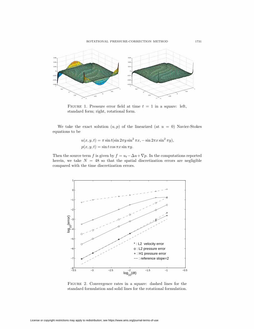
Figure 1. Pressure error field at time t = 1 in a square: left,standard form; right, rotational form.

We take the exact solution (u, p) of the linearized (at u = 0) Navier-Stokesequations to be

u(x, y, t) = π sin t(sin 2πy sin2 πx,− sin 2πx sin2 πy),

p(x, y, t) = sin t cosπx sinπy.

Then the source term f is given by f = ut−∆u+∇p. In the computations reportedherein, we take N = 48 so that the spatial discretization errors are negligiblecompared with the time discretization errors.

−3.5 −3 −2.5 −2 −1.5 −1 −0.5−8

−7

−6

−5

−4

−3

−2

−1

0

1

log10

(dt)

log 10

(err

or)

* : L2 velocity error o : L2 pressure error + : H1 pressure error −− : reference slope=2

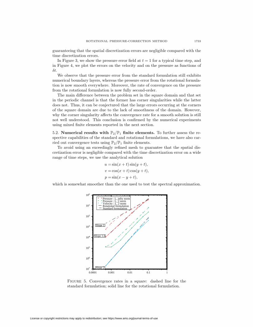
Figure 2. Convergence rates in a square: dashed lines for thestandard formulation and solid lines for the rotational formulation.



In Figure 1, we plot the pressure error field at t = 1 for a typical time step,and in Figure 2, we represent errors on the pressure and the velocity measured invarious norms as functions of the time step δt.

We note in Figure 1 that for the standard form of the algorithm, a numericalboundary layer appears on the two boundaries (x, y) : x ∈ (−1, 1), y = ±1 wherethe exact pressure is such that ∂p

∂~n 6= 0 ( ∂p∂~n = 0 on the other two boundaries). Forthe rotational form, there is no numerical boundary layer, but we observe largespikes at the four corners of the domain. These observations suggest that thedivergence correction in the rotational form, which leads to consistent approximatepressure Neumann boundary conditions, successfully cured the numerical boundarylayer problem. However, the large errors at the four corners degrade the globalconvergence rate of the pressure approximation. Indeed, we observe in Figure 2that the pressure approximation from the rotational formulation is not fully second-order accurate, though it is significantly more accurate than that calculated usingthe standard formulation. We also note that the rotational formulation does notyield any improvement on the approximation of the velocity in the L2-norm.

To better understand why there are localized large errors at the corners of the do-main, we have also implemented the standard and rotational forms of the pressure-correction scheme in a periodic channel Ω = (0, 2π)× (−1, 1). We assume that thesolution is periodic in the x direction and that the velocity is subject to a Dirichletboundary condition at y = ±1. We choose the same exact solution (u, p) as givenabove, and we use a Fourier-Legendre spectral approximation with 48× 49 modes

Figure 3. Error field on pressure at time t = 1 in a channel: left,standard form; right, rotational form.

−3.5 −3 −2.5 −2 −1.5 −1 −0.5−9

−8

−7

−6

−5

−4

−3

−2

−1

0

log10

(dt)

log 10

(err

or)

o : L2 pressure error v : Maximum pressure error * : L2 velocity error * : Maximum velocity error −− : reference slope=2

−3.5 −3 −2.5 −2 −1.5 −1 −0.5−9

−8

−7

−6

−5

−4

−3

−2

log10

(dt)

log 10

(err

or)

o : L2 pressure error

v : Maximum pressure error

* : L2 velocity error

* : Maximum velocity error

−− : reference slope=2

Figure 4. Convergence rates in a periodic channel: left, standardform; right, rotational form.



guaranteeing that the spatial discretization errors are negligible compared with thetime discretization errors.

In Figure 3, we show the pressure error field at t = 1 for a typical time step, andin Figure 4, we plot the errors on the velocity and on the pressure as functions ofδt.

We observe that the pressure error from the standard formulation still exhibitsnumerical boundary layers, whereas the pressure error from the rotational formula-tion is now smooth everywhere. Moreover, the rate of convergence on the pressurefrom the rotational formulation is now fully second-order.

The main difference between the problem set in the square domain and that setin the periodic channel is that the former has corner singularities while the latterdoes not. Thus, it can be conjectured that the large errors occurring at the cornersof the square domain are due to the lack of smoothness of the domain. However,why the corner singularity affects the convergence rate for a smooth solution is stillnot well understood. This conclusion is confirmed by the numerical experimentsusing mixed finite elements reported in the next section.

5.2. Numerical results with P2/P1 finite elements. To further assess the re-spective capabilities of the standard and rotational formulations, we have also car-ried out convergence tests using P2/P1 finite elements.

To avoid using an exceedingly refined mesh to guarantee that the spatial dis-cretization error is negligible compared with the time discretization error on a widerange of time steps, we use the analytical solution

u = sin(x+ t) sin(y + t),

v = cos(x + t) cos(y + t),

p = sin(x− y + t),

which is somewhat smoother than the one used to test the spectral approximation.

0.0001 0.001 0.01 0.1 1107

106

105

104

103

102

101

100

Pressure : L_infty normPressure : L_2 norm Velocity : L_2 norm Rotational formulation Standard formulation

Slope 1

Slope 1.6

Slope 2

Figure 5. Convergence rates in a square: dashed line for thestandard formulation; solid line for the rotational formulation.



Figure 6. Error field on pressure in a rectangular domain: left,standard formulation; right, rotational formulation.

The domain considered to perform the convergence tests is the square (0, 1)2. Weused a P2/P1 mesh composed of 14774 elements (7548 P1 nodes and 29869 P2 nodes)corresponding to the average mesh size h = 1/80. In Figure 5, we show the error onthe velocity in the L2-norm and that on the pressure in the L2-norm and L∞-norm.The errors are measured at time t = 1. The conclusions are essentially the sameas that from the tests with the spectral approximation. The rate on the velocity isclearly second-order, and the rotational formulation does not significantly improvethe accuracy on the velocity, though the error produced is systematically lower thanthat from the standard formulation. Concerning the pressure, the convergence rateson the errors in the L2-norm are slightly lower than second-order for both forms ofthe algorithm, the rotational form systematically producing better results though.The slight saturation of the errors for very small time steps is due to the spatialinterpolation error that becomes visible. For the L∞-norm, the convergence ratesare obviously different. It is 1.6 for the rotational formulation and first-order for thestandard formulation, with the departure from first-order for small time steps dueto nonuniform inverse estimates as we have verified that the position of departuremoves to the left when the mesh is refined.

We show in Figure 6 the error fields on the pressure at time t = 1 for δt = 0.00625.As for the spectral approximation, we note that the rotational form of the algorithmyields a pressure field that is free of a numerical boundary layer, whereas a boundarylayer is clearly visible on the pressure field obtained by means of the standardalgorithm. We note also that large errors are still present at the corners of thedomain for both formulations.

To clarify the effect of the smoothness of the boundary on the error on the pres-sure, we have tested the two methods on the circular domain Ω = (x, y);

√x2 + y2

≤ 0.5, using the same analytical solution as before and h = 1/80. We show in Fig-ure 7 the error field on the pressure for δt = 0.0125 at t = 2. A numerical boundarylayer is clearly visible on the entire boundary for the pressure calculated by meansof the standard formulation, but the error is uniformly small for the pressure cal-culated using the rotational formulation. This test confirms that the smoothnessof the boundary has a very important impact on the quality of the approximationoffered by the rotational formulation.



Figure 7. Error field on pressure in a circular domain: left, stan-dard formulation; right, rotational formulation.

This point is made even more clear in Figure 8. In the left graph of the figure,we show the convergence rates on the velocity in the L2-norm and that on thepressure in the L2-norm and L∞-norm, with the error measured at time t = 2.The convergence rates are all second-order for the rotational formulation, whereasthis is not the case for the standard one. In the graph in the right panel of thefigure, we compare the convergence rates on the pressure in the L∞-norm for therotational formulation only, one series of computation being made on the squareand the other on the circle. It is clear that the errors calculated on the circulardomain are O(δt2), whereas those calculated on the square are only O(δt1.6).

Figure 8. Left: convergence rates on a circular domain; dashedlines for the standard formulation; solid lines for the rotationalformulation. Right: comparison of convergence rates on pressurein L∞-norm; solid line for the circular domain; dashed line for thesquare.



5.3. Discussions on the convergence rates of the pressure approximations.There exists in the literature a substantial number of works dedicated to numer-ical and theoretical investigations on the convergence rates of the pressure usingpressure-correction schemes. For the standard form, first-order error estimates onthe pressure are established in [12, 15] for the semi-discrete case and in [7] for thefully discrete case. These results are valid in fairly general domains such as con-vex polygons. In [4], E and Liu, using asymptotic analysis in a periodic channel,obtained for the standard formulation a first-order error estimate on the pressurein the L∞-norm. All these results are consistent with the claim of Strikwerda andLee in [16] that the pressure approximation in the standard formulation can be atmost first-order accurate. This claim is based on a normal mode analysis in thehalf-plane.

In [1], using a normal mode analysis in a periodic channel, Brown, Cortez andMinion showed that the pressure approximation in the rotational formulation issecond-order accurate. This is consistent with our numerical results in a periodicchannel as well, but unfortunately, this result does not hold for general domainsas is evidenced by our numerical results. Therefore, it seems that the convergencerate of 3

2 we established here for the pressure approximation in rotational form isthe best possible for general domains.

References

1. David L. Brown, Ricardo Cortez, and Michael L. Minion. Accurate projection methods forthe incompressible Navier-Stokes equations. J. Comput. Phys., 168(2):464–499, 2001. MR2002a:76112

2. A. J. Chorin. Numerical solution of the Navier-Stokes equations. Math. Comp., 22:745–762,1968. MR 39:3723

3. A. J. Chorin. On the convergence of discrete approximations to the Navier-Stokes equations.Math. Comp., 23:341–353, 1969. MR 39:3724

4. W. E and J.G. Liu. Projection method I: Convergence and numerical boundary layers. SIAMJ. Numer. Anal., 32:1017–1057, 1995. MR 96e:65061

5. W. E and J.G. Liu. Projection method. III. Spatial discretization on the staggered grid. Math.Comp., 71(237):27–47, 2002. MR 2002k:65155

6. K. Goda. A multistep technique with implicit difference schemes for calculating two- or three-dimensional cavity flows. J. Comput. Phys., 30:76–95, 1979.

7. J.-L. Guermond. Un resultat de convergence a l’ordre deux en temps pour l’approximationdes equations de Navier–Stokes par une technique de projection. Model. Math. Anal. Numer.(M2AN), 33(1):169–189, 1999. MR 2000k:65171

8. J.L. Guermond and Jie Shen. Velocity-correction projection methods for incompressible flows.To appear in SIAM J. Numer. Anal.

9. G. E. Karniadakis, M. Israeli, and S. A. Orszag. High-order splitting methods for the incom-pressible Navier-Stokes equations. J. Comput. Phys., 97:414–443, 1991. MR 92h:76066

10. S. A. Orszag, M. Israeli, and M. Deville. Boundary conditions for incompressible flows. J. Sci.Comput., 1:75–111, 1986.

11. R. Rannacher. On Chorin’s projection method for the incompressible Navier-Stokes equations.Lecture Notes in Mathematics, vol. 1530, 1991. MR 95a:65149

12. Jie Shen. On error estimates of the projection methods for the Navier-Stokes equations: first-order schemes. SIAM J. Numer. Anal., 29:57–77, 1992. MR 92m:35213

13. Jie Shen. On pressure stabilization method and projection method for unsteady Navier-Stokesequations. In R. Vichnevetsky, D. Knight, and G. Richter, editors, Advances in Computer

Methods for Partial Differential Equations, pages 658–662, IMACS, 1992.14. Jie Shen. Efficient spectral-Galerkin method I. direct solvers for second- and fourth-order

equations by using Legendre polynomials. SIAM J. Sci. Comput., 15:1489–1505, 1994. MR95j:65150


http://www.ams.org/mathscinet-getitem?mr=2002a:76112

http://www.ams.org/mathscinet-getitem?mr=39:3723


http://www.ams.org/mathscinet-getitem?mr=96e:65061

http://www.ams.org/mathscinet-getitem?mr=2002k:65155

http://www.ams.org/mathscinet-getitem?mr=2000k:65171

http://www.ams.org/mathscinet-getitem?mr=92h:76066

http://www.ams.org/mathscinet-getitem?mr=95a:65149

http://www.ams.org/mathscinet-getitem?mr=92m:35213

http://www.ams.org/mathscinet-getitem?mr=95j:65150


15. Jie Shen. On error estimates of projection methods for the Navier-Stokes equations: second-order schemes. Math. Comp, 65:1039–1065, July 1996. MR 96j:65091

16. J. C. Strikwerda and Y. S. Lee. The accuracy of the fractional step method. SIAM J. Numer.Anal., 37(1):37–47, 1999. MR 2000h:65127

17. R. Temam. Sur l’approximation de la solution des equations de Navier-Stokes par la methodedes pas fractionnaires ii. Arch. Rat. Mech. Anal., 33:377–385, 1969. MR 39:5968

18. R. Temam. Navier-Stokes Equations: Theory and Numerical Analysis. North-Holland, Ams-terdam, 1984. MR 58:29439

19. L. J. P. Timmermans, P. D. Minev, and F. N. Van De Vosse. An approximate projec-tion scheme for incompressible flow using spectral elements. Int. J. Numer. Methods Fluids,22:673–688, 1996.

20. J. van Kan. A second-order accurate pressure-correction scheme for viscous incompressibleflow. SIAM J. Sci. Stat. Comput., 7:870–891, 1986. MR 87h:76008

LIMSI (CNRS-UPR 3152), BP 133, 91403, Orsay, France

E-mail address: [email protected]

Department of Mathematics, Purdue University, West Lafayette, Indiana 47907

E-mail address: [email protected]


http://www.ams.org/mathscinet-getitem?mr=96j:65091





Documents

ON THE ERROR ESTIMATES FOR THE ROTATIONAL PRESSURE-CORRECTION … · 2018-11-16 · MATHEMATICS OF COMPUTATION Volume 73, Number 248, Pages 1719{1737 S 0025-5718(03)01621-1 Article