Embed Size (px)
Citation preview

NCER Working Paper SeriesNCER Working Paper Series
On the Efficacy of Fourier Series Approximations for Pricing European and Digital Options
A S HurnA S Hurn K A LindsayK A Lindsay A J McClellandA J McClelland Working Paper #90Working Paper #90 January 2013January 2013
ON THE EFFICACY OF FOURIER SERIES APPROXIMATIONSFOR PRICING EUROPEAN AND DIGITAL OPTIONS
A. S. HURN∗, K. A. LINDSAY† , AND A. J. MCCLELLAND‡
Abstract. This paper investigates several competing procedures for computing the price ofEuropean and digital options in which the underlying model has a characteristic function that isknown in at least semi-closed form. The algorithms for pricing the options investigated here arethe half-range Fourier cosine series, the half-range Fourier sine series and the full-range Fourierseries. The performance of the algorithms is assessed in simulation experiments which price optionsin a Black-Scholes world where an analytical solution is available and for a simple affine model ofstochastic volatility in which there is no closed-form solution. The results suggest that the half-rangesine series approximation is the least effective of the three proposed algorithms. It is rather moredifficult to distinguish between the performance of the half-range cosine series and the full-rangeFourier series. There are however two clear differences. First, when the interval over which thedensity is approximated is relatively large, the full-range Fourier series is at least as good as thehalf-range Fourier cosine series, and outperforms the latter in pricing out-of-the-money call options,in particular with maturities of three months or less. Second, the computational time required bythe half-range Fourier cosine series is uniformly longer than that required by the full-range Fourierseries for an interval of fixed length. Taken together, these two conclusions make a strong case forthe merit of pricing options using a full-range range Fourier series as opposed to a half-range Fouriercosine series.
Key words. Fourier transform, Fourier series, characteristic function, option price
AMS subject classifications. 62P05, 91G20, 91G60
∗School of Economics and Finance, Queensland University of Technology†School of Mathematics and Statistics, University of Glasgow and School of Economics and Fi-
nance, Queensland University of Technology‡Sydney Numerix
2 HURN, LINDSAY AND MCCLELLAND
1. Introduction. This paper investigates several competing procedures for com-puting the price of European and digital options. This problem has received newimpetus in recent years with the development of particle filtering approaches to theestimation of stochastic volatility models. This procedure allows time-series returnsdata to be combined with cross-sectional options data at each point in time [11], [3],[5], [10]. The computational complexity of this approach is driven by the requirementthat each function evaluation of a search algorithm involves the calculation of around1 billion model option prices when estimating simple models with reasonable amountsof data. On a desktop PC a realistic outcome is one function evaluation per day, whichimplies one full model estimation every 6 months or so thereby rendering any estima-tion exercise infeasible. The innovations that allow this kind of computation to bereduced to a matter of hours as opposed to months stems from the fact that a particlefiltering algorithm lends itself to parallel computation. Indeed, in the parlance ofcomputer theorists the problem is “embarrassingly parallel” and computation in thiskind of environment is becoming increasingly of interest [6], [7].
While major advances are being made in computational speed due to parallelisation ongraphical processing units (GPU), the fact remains that the major numerical effort inestimating the parameters of stochastic volatility models resides in the computationalload arising from the need to price large numbers of options with various strike pricesand maturities, not to mention the management of daily changes in the value of therisk-free rate of interest. The ability to price options accurately and efficiently cannotbe overestimated and re-visiting this issue is timely.
Various strategies have been proposed for calculating the price of option contractsfrom knowledge of the conditional characteristic function of the underlying model. Itis an important fact that a surprisingly large number of models have a semi-closedexpression for their conditional characteristic function. For example, the identificationof the conditional characteristic function for multivariate affine models with/withoutjump processes leads to the solution of a family of ordinary differential equations,albeit in the complex plane. In view of the Levy-Khintchine theorem, the identificationof the conditional characteristic function for Levy processes is expressed in terms ofvarious integrals with respect to the Levy measure.
The most commonly used techniques for taking advantage of a known conditionalcharacteristic function have at their core the application of the Fast Fourier Trans-form (FFT). The most well documented of these approaches is due to Carr and Madan[4] who construct an expression for the price of a European call option in terms of anintegral over the characteristic function. This integral, which has an oscillatory ker-nel, is computed by an application of the FFT. Borak, Detlefsen and Hardle [2] applythe FFT strategy and demonstrate its efficacy by comparison with Monte Carlo sim-ulation for a variety of models. Lord, Fang, Bervoets and Oosterlee [13] and Kwok,Leung and Wong [12] demonstrate how Fourier’s convolution theorem in combina-tion with the FFT can be used to price certain exotic options from knowledge ofthe conditional characteristic function of the price of the underlying asset. A dif-ferent approach pioneered by Fang and Oosterlee [8] uses the characteristic functionto directly approximate the marginal transitional probability density of returns by aFourier cosine series. More recently Zhang, Grzelak and Oosterlee [14] demonstratehow this methodology can be extended to the pricing of early-exercise commodityoptions under the Ornstein-Uhlenbeck process.
Rather than describe in detail the nuances of these various strategies, it is useful to
OPTION PRICING 3
point out what overarching assumptions connect them. Recall that the FFT is simplya clever piece of linear algebra that reduces the arithmetical load in implementingthe Discrete Fourier Transform (DFT), namely the pair of equations connecting thecoefficients of a finite Fourier series with values of the underlying function and viceversa. Therefore the decision to use the FFT implicitly makes the assumption that theunderlying function is periodic over an interval of finite length, in practice determinedby the frequencies submitted to the characteristic function, and that the function hasbeen approximated over the interval by a finite Fourier series. The values of Fouriercoefficients calculated from the characteristic function are in error by the extent towhich the finite Fourier transform1 differs from the Fourier transform.
Thus techniques using the FFT and those based on the construction of Fourier seriesshare the same common assumptions and deficiencies. However, an important differ-ence between an implementation using the FFT approach and one using the Fourierseries approach is that the latter is parsimonious in its use of arithmetic whereasthe former typically performs more arithmetic than is necessary, albeit in an efficientway. For example, if the FFT is used to determine the value of a probability densityfunction what is recovered is the value of the function at each node of the interval,whereas all that what might be needed is the value of the probability density functionover a sub-interval.
The focus of this work is on the algorithm proposed by Fang and Oosterlee [8] whogive a convincing demonstration of the efficacy of the Fourier cosine series. This seriesis more accurately called the half-range2 cosine series because the actual function tobe expanded is defined only on half the interval of periodicity (or range), the functionbeing extended to the full range as an even-valued function. Half-range cosine seriesusually fail to represent derivatives whereas half-range Fourier series usually fail torepresent function values. While the use of the half-range Fourier cosine series is a solididea, Fang and Oosterlee Fang and Oosterlee [8] provide no motivation or explanationas to why this choice of approximating transitional density should be preferred overthe half-range Fourier sine series or the full-range Fourier series for that matter. Forexample, intuition would suggest that the latter might perform better simply becauseit uses higher frequencies which in turn translate to a more rapidly converging Fourierexpansion. Indeed this intuition is borne out in calculation, but of course speed is notthe only criterion of relevance in assessing the efficacy of a numerical procedure.
An important but subtle difference between the half-range cosine series and full-range Fourier series approximations of density and that based on the half-range sineseries is that the former assign unit probability to the interval of support when inreality probability lies outside this interval, whereas the latter imposes zero probabilitydensity at the endpoints of the interval of support in contravention of reality, but onthe other hand does not assign unit probability to the interval of support. Is oneapproach always superior to the other or is it a case of horses for courses? Intuitionmight suggest the latter. For example, when pricing a call option the most importantcomponent of the pricing error comes from the exclusion of contributions from assetprice exterior to the finite interval of support. Because the half-range cosine andfull-range Fourier series necessarily capture unit density, intuition might suggest thatthese approximations provide potential compensation for this component of pricing
1The finite Fourier transform is the integral expression defining the coefficients of a Fourier series.2Historically, half-range Fourier series largely arise as analytical tools for handling different types
of boundary conditions when solving partial differential equations using integral transforms.
4 HURN, LINDSAY AND MCCLELLAND
error. On the other hand intuition would suggest that the same approximations, whenused to price digital options, might have a tendency to exaggerate the probability ofexercise and therefore overprice this option in contrast to the half-range sine seriesapproximation of probability density.
2. Fourier series and transform. Suppose that f(y) satisfies the Dirichletconditions on [a, b ], then there are three common ways in which f(y) may be repre-sented by a Fourier series. These are the half-range Fourier cosine series, the half-rangeFourier sine series and the full-range Fourier series with their respective representa-tions
(a)a02
+
∞∑k=1
ak cos(kπ(y − a)
b− a
),
(b)
∞∑k=1
bk sin(kπ(y − a)
b− a
),
(c)a02
+
∞∑k=1
ak cos(2kπ(y − a)
b− a
)+ bk sin
(2kπ(y − a)
b− a
).
(2.1)
The use of the term “half-range” in describing expressions (a) and (b) simply refers tothe fact that the function f(y), although defined in [a, b ], has for the construction ofthe Fourier series been extended into the interval [2a−b, a] as an even-valued functionin the case of the half-range cosine series (so that sine contributions vanish) and as anodd-valued function in the case of the half-range sine series (so that the constant andcosine contributions vanish). Thus both half-range series are conventional Fourierseries taken over the interval [2a − b, b ] such that the function represented by thehalf-range Fourier cosine series is usually not differentiable at x = a, whereas thatrepresented by the half-range Fourier sine series is usually discontinuous at x = a.
In the case of the half-range cosine and sine series in expressions (2.1a) and (2.1b)respectively, the coefficients ak (k ≥ 0) and bk (k ≥ 1) are calculated from the functionf(y) via the formulae
ak =2
b− a
∫ b
a
f(y) cos(kπ(y − a)
b− a
)dy
bk =2
b− a
∫ b
a
f(y) sin(kπ(y − a)
b− a
)dy .
(2.2)
When expressed in terms of the exponential function the coefficients ak and bk become
ak =2
b− a
∫ b
a
<[f(y) exp
( kπiyb− a
)exp
(−kπiab− a
)dy],
bk =2
b− a
∫ b
a
=[f(y) exp
( kπiyb− a
)exp
(−kπiab− a
)dy].
(2.3)
In the case of the full-range Fourier series in expression (2.1c) the coefficients ak(k ≥ 0) and bk (k ≥ 1) are calculated from the function f(y) via the formulae
ak =1
b− a
∫ b
a
f(y) cos(2kπ(y − a)
b− a
)dy ,
bk =1
b− a
∫ b
a
f(y) sin(2kπ(y − a)
b− a
)dy
(2.4)
OPTION PRICING 5
both of which can be brought together in the single complex expression
ak + ibk =1
b− a
∫ b
a
f(y) exp(2kπiy
b− a
)exp
(−2kπia
b− a
)dy . (2.5)
Suppose now that f(y) is a transitional probability density function with known char-acteristic function defined formally by the equation
χ(ω) = E[ e iωy ] =
∫Rf(y) eiωy dy , (2.6)
where ω ∈ R and χ(0) = 1 irrespective of the specification of the density f(y). Anecessary condition for f(y) to be a probability density function is that f(y)→ 0 as| y | → ∞, and therefore there is guaranteed to be an interval [a, b] such that for ally ∈ (−∞, a]∪ [b,∞) it can be asserted that f(y) < ε for any arbitrary small positive ε.The implication of this observation is that the Fourier coefficients in equations (2.3)and (2.5) can be approximated from knowledge of the characteristic function via therespective formulae
ak ≈ Ak =2
b− a<[χ( kπ
b− a
)exp
(−kπiab− a
) ],
bk ≈ Bk =2
b− a=[χ( kπ
b− a
)exp
(−kπiab− a
) ],
(2.7)
while the coefficients of the full-range Fourier series can be approximated from knowl-edge of the characteristic function via the formula
ak + ibk ≈ Ak + iBk =1
b− aχ( 2kπ
b− a
)exp
(−2kπia
b− a
). (2.8)
The accuracy of approximations (2.7) and (2.8) is investigated in Section 6, where itis demonstrated that the error can be made arbitrarily small by choosing a suitablylarge interval.
3. Approximating Probability Density Functions. The quality of this prac-tical idea is now explored for three trial probability density functions with knownclosed-form expressions for their characteristic functions. The first choice is the Gaus-sian density which may be regarded as representative of distributions with super-exponentially decaying tail density. The second and third choices are the Gammadensity and the Cauchy density which are treated as representative examples of dis-tributions with exponentially decaying and algebraically decaying tail density respec-tively.
3.1. Gaussian density. It is standard knowledge that the Gaussian densitywith mean value µ and variance σ2 has characteristic function χ(ω) = exp
(i µ ω −
σ2ω2/2)
which corresponds to the equivalent specifications cn = exp(−σ2k2n/2) cos(µkn)and sn = exp(−σ2k2n/2) sin(µkn). In order to demonstrate the quality with which thetrue probability density f(x) can be reconstructed from a truncated Fourier series ofthe form of equation (2.1 c), suppose that µ = σ = 1 and take the interval of supportto be [a, b ] = [−3, 5], i.e. four standard deviations on either side of the mean value.The approximating function in this case using N/2 frequencies is
f̂(x) =1
8
[c0 + 2
N/2∑n=1
(cn cos knx+ sn sin knx
)], kn =
nπ
4. (3.1)
6 HURN, LINDSAY AND MCCLELLAND
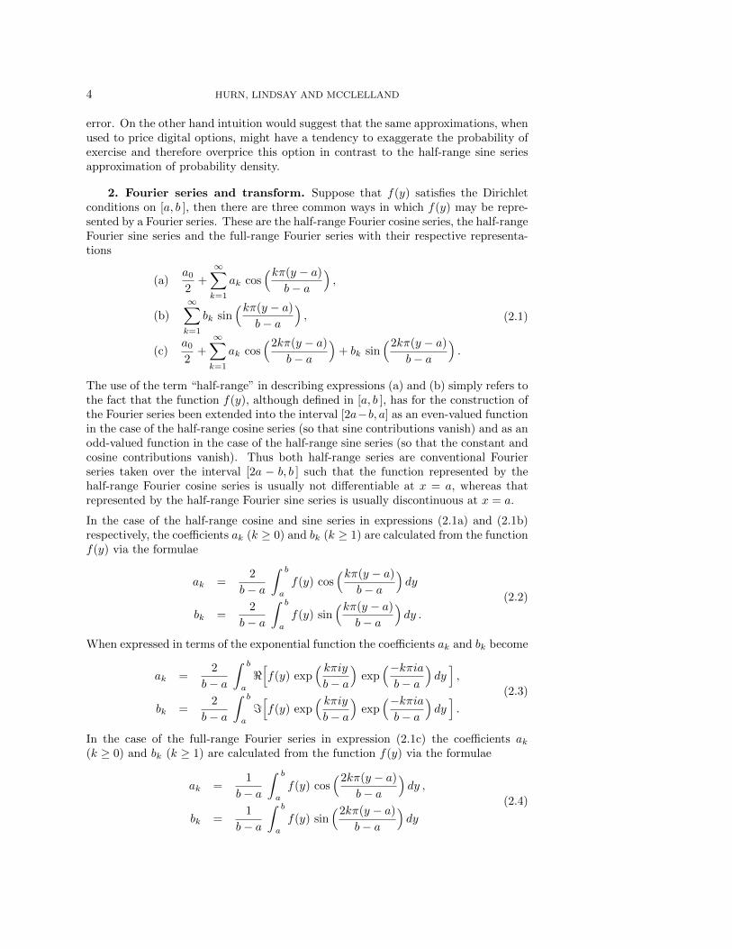
Figure 3.1 illustrates the quality of this approximation using 40 frequencies (N = 80)and using 4 frequencies (N = 8).
-3 -2 -1 0 1 2 3 4 5
0.1
0.2
0.3
0.4
Fig. 3.1. Comparison of the true Gaussian density and its approximation based on40 frequencies (solid line, N = 80) and 4 frequencies (dashed line, N = 8)
With as few as 4 frequencies it is clear that the approximating density still provides agood representation of the true density; with 40 frequencies the approximating densityfunction is indistinguishable from the true density function. The explanation of thisexcellent performance stems from the property that the error bound F (a) + 1− F (b)converges to zero super-exponentially as a→ −∞ and b→∞.
3.2. Gamma density. The Gamma density with shape parameter α and scaleparameter β has probability density function and characteristic function give by therespective formulae
f(x) =1
Γ(α)β
(xβ
)α−1e−x/β , χ(ω) =
1
(1− iβω)α. (3.2)
The approximating density is identical to expression (3.1) with b− a = 8 but now
cn =cos(α tan−1 βkn)
(1 + β2k2n)α/2, sn =
sin(α tan−1 βkn)
(1 + β2k2n)α/2.
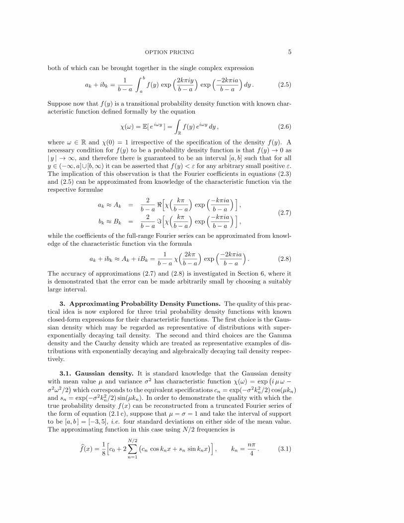
The task is again to reconstruct the Gamma probability density function from χ(ω).The fact that the deviate Y = X/β is also Gamma distributed, in this case with shapeparameter α and unit scale parameter, suggest that for the Gamma distribution theappropriate comparison is between the approximating Fourier series and a Gammadistribution with unit scale parameter. Figure 3.2 illustrates the quality of this ap-proximation for Γ( 3
2 , 1) for 50 frequencies (solid line, N = 100) and 20 frequencies(dashed line, N = 40). With the exception of the region very close to the origin,the true density and approximated density are not significantly different for even 20frequencies, and with 50 frequencies the difference between the true density and theapproximating density is not discernible with the exception of the origin which doesnot present a difficulty since the density to known to be zero there.
OPTION PRICING 7
0 1 2 3 4 5 6 7 80.0
0.1
0.2
0.3
0.4
0.5
Fig. 3.2. Comparison of the Gamma density Γ(3/2, 1) and its approximations basedon 50 frequencies (solid line, N = 100) and 20 frequencies (dashed line, N = 40)
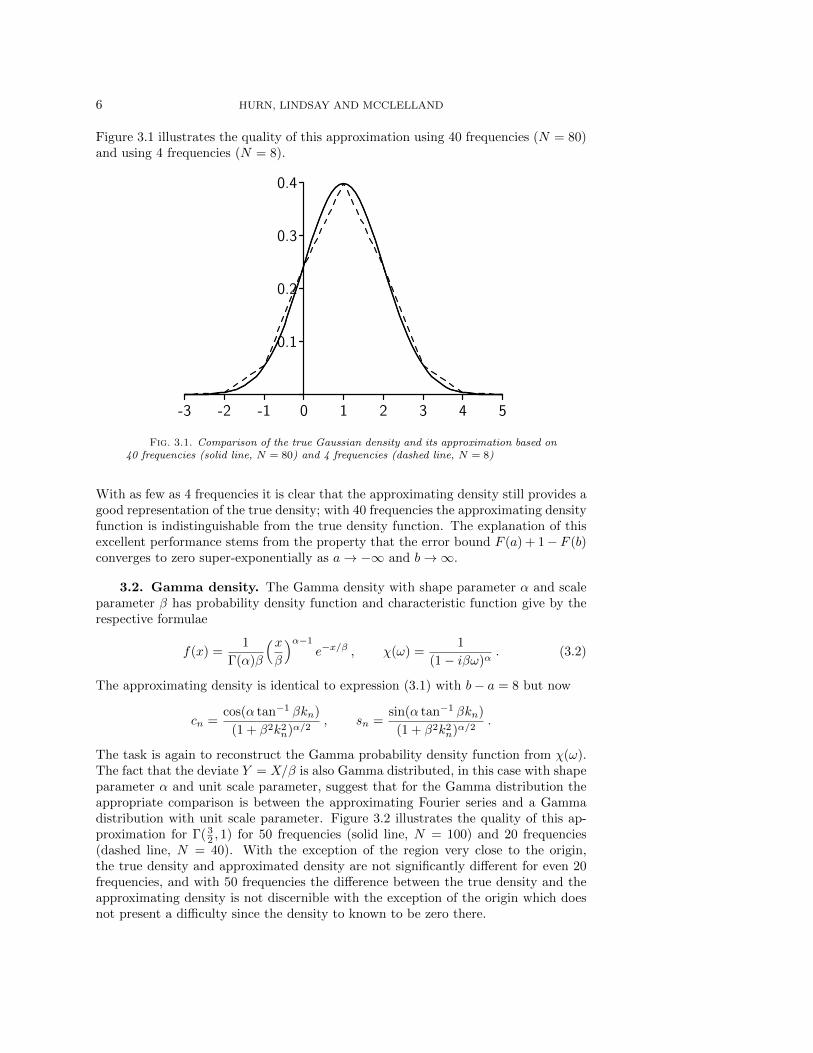
The quality of the approximation is again due to the fact that the error bound 1−F (b)converges to zero exponentially as b→∞. Typical values for the coefficient of meanreversion (say, κ = 3.0), the mean volatility (say γ = 0.02) and the volatility ofvolatility (say σ = 0.2) in Heston’s model of stochastic volatility lead to a stationarydistribution of volatility described by a Gamma density with shape parameter α =2κγ/σ2 = 3.0. A second example with α = 3 and β = 1 is illustrated in Figure 3.3.
0 1 2 3 4 5 6 7 80.0
0.1
0.2
0.3
Fig. 3.3. Comparison of the Gamma density Γ(3, 1) (solid line) and its approxi-mations based on 10 frequencies (dashed line, N = 20)
The important observation from both of these experiments is that distributions withexponentially decaying tail density can be well described by a relatively small bandof frequencies.
3.3. Cauchy density. The Cauchy density with median µ and scale parameterα has probability density function and characteristic function give by the respectiveformulae
f(x) =α
π
1
(x− µ)2 + α2, χ(ω) = eiµω−α |ω| . (3.3)
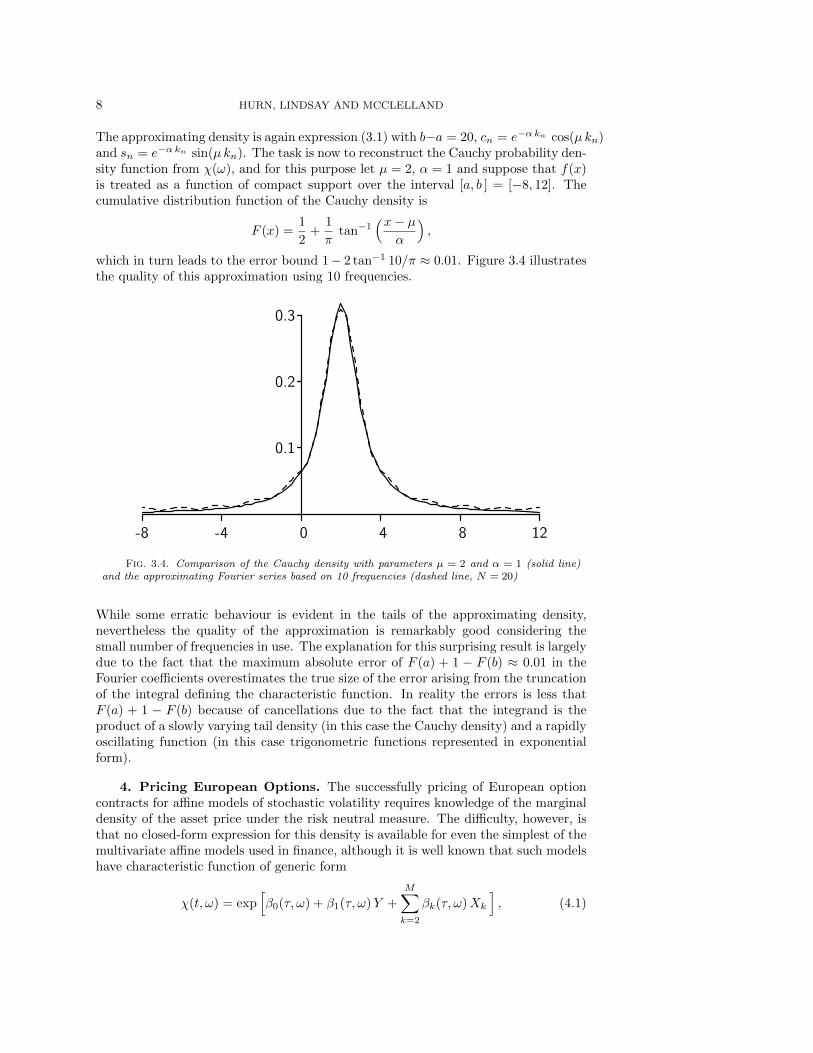
8 HURN, LINDSAY AND MCCLELLAND
The approximating density is again expression (3.1) with b−a = 20, cn = e−αkn cos(µkn)and sn = e−αkn sin(µkn). The task is now to reconstruct the Cauchy probability den-sity function from χ(ω), and for this purpose let µ = 2, α = 1 and suppose that f(x)is treated as a function of compact support over the interval [a, b ] = [−8, 12]. Thecumulative distribution function of the Cauchy density is
F (x) =1
2+
1
πtan−1
(x− µα
),
which in turn leads to the error bound 1− 2 tan−1 10/π ≈ 0.01. Figure 3.4 illustratesthe quality of this approximation using 10 frequencies.
-8 -4 0 4 8 12
0.1
0.2
0.3
Fig. 3.4. Comparison of the Cauchy density with parameters µ = 2 and α = 1 (solid line)and the approximating Fourier series based on 10 frequencies (dashed line, N = 20)
While some erratic behaviour is evident in the tails of the approximating density,nevertheless the quality of the approximation is remarkably good considering thesmall number of frequencies in use. The explanation for this surprising result is largelydue to the fact that the maximum absolute error of F (a) + 1 − F (b) ≈ 0.01 in theFourier coefficients overestimates the true size of the error arising from the truncationof the integral defining the characteristic function. In reality the errors is less thatF (a) + 1 − F (b) because of cancellations due to the fact that the integrand is theproduct of a slowly varying tail density (in this case the Cauchy density) and a rapidlyoscillating function (in this case trigonometric functions represented in exponentialform).
4. Pricing European Options. The successfully pricing of European optioncontracts for affine models of stochastic volatility requires knowledge of the marginaldensity of the asset price under the risk neutral measure. The difficulty, however, isthat no closed-form expression for this density is available for even the simplest of themultivariate affine models used in finance, although it is well known that such modelshave characteristic function of generic form
χ(t, ω) = exp[β0(τ, ω) + β1(τ, ω)Y +
M∑k=2
βk(τ, ω)Xk
], (4.1)
OPTION PRICING 9
where T is the maturity of the option, τ = T − t is the backward variable and ω is thecharacteristic variable associated with the non-dimensional variable Y , here definedto be the logarithm of the ratio of asset price to strike price. The state variablesX =
(X2, · · · , XM
)in expression (4.1) denote the values of the latent states of the
system at time t. Typically the functions β0, · · · , βM are the solution of a systemof (M + 1) ordinary differential equations with initial conditions β1(0, ω) = iω andβ0(0, ω) = β2(0, ω), · · · , βM (0, ω) = 0. In overview, there is a well trodden procedurethat starts with the specification of the multivariate affine model and ends with theconstruction of χ(t, ω).
4.1. European call option. In the case of a European call option with strikeprice K and maturity T on an asset with spot price S0, the price of the option is
e−rT∫ ∞K
(S −K)f̃Q(S0, X2 · · ·XM , T∣∣S; θ) dS ,
where f̃Q(S0, X2 · · ·XM , T∣∣S; θ) is the marginal density of the asset price at the
maturity of the option when S0 is the spot price of the asset and (X2, · · · , XM ) arethe spot values of the latent states. When expressed in terms of y = log(S/K), theprice of the option becomes
C = e−rTK
∫ ∞0
(ey − 1) fQ(ξ,X2 · · ·XM , T∣∣ y; θ) dy , (4.2)
where ξ = log(S0/K). The value of this integral is now approximated under the as-sumption that fQ(ξ,X2 · · ·XM , T
∣∣ y; θ) is well approximated by a function of compactsupport over the interval [a, b ]. Of course, the specific form taken by this approxi-mation will depend of the choice of expression (a), (b) or (c) in equations (2.1), butin each case the approximation of fQ(ξ,X2 · · ·XM , T
∣∣ y; θ) by a function of compactsupport in [a, b ] necessarily changes the interval of integration in expression (4.2) from[0,∞) to [0, b ]. Thereafter it is straightforward Calculus to show that the cost of acall option on the basis of approximations (a) and (b) is
(a) C = e−rTK[a0
2
(eb − b− 1
)+
∞∑k=1
akωke
b(−1)k − ωk cosωka− sinωka
ωk(1 + ω2k)
],
(b) C = e−rTK[ ∞∑k=1
bkωk
((eb − 1)(−1)k−1 +
ωk sinωka− cosωka+ eb(−1)k
1 + ω2k
)],
(4.3)where ωk = kπ/(b− a). Based on approximation (c) the price of a call option is
(c) C = e−rTK[a0
2
(eb − b− 1
)+
∞∑k=1
akλke
b − λk cosλka− sinλka
λk(1 + λ2k)
+bkλk
(1− eb +
λk sinλka− cosλka+ eb
1 + λ2k
)],
(4.4)
where λk = 2kπ/(b − a). The primary computational load in the computation ofexpressions (a), (b) and (c) resides in the calculation of trigonometric functions, andconsequently individual terms of expression (c) require more arithmetical effort thanthe equivalent terms of either expression (a) or (b). However this difference in com-putational load is insignificant when compared with the more rapid convergence of
10 HURN, LINDSAY AND MCCLELLAND
summation (c) compared with that of summations (a) and (b) due entirely to thefact that the frequencies used in approximation (c) are exactly double those used inapproximations (a) and (b).
4.2. Digital option. The price of a digital option with strike price K and ma-turity T on an asset with spot price S0 is
e−rT∫ ∞K
f̃Q(S0, X2 · · ·XM , T∣∣S; θ) dS ,
where f̃Q(S0, X2 · · ·XM , T∣∣S; θ) is the marginal density of the asset price at the
maturity of the option when the asset has spot price S0 and (X2, · · · , XM ) are thespot values of the latent states. When expressed in terms of the y = log(S/K), theprice of the digital becomes
D = e−rT∫ ∞0
fQ(ξ,X2 · · ·XM , T∣∣ y; θ) dy , (4.5)
where ξ = log(S0/K). The value of this integral is now approximated under the as-sumption that fQ(ξ,X2 · · ·XM , T
∣∣ y; θ) is well represented by the procedures proposedin Section 2. Specifically, the price of a digital option computed from the half-rangecosine, half-range sine and full-range Fourier series are respectively
(a) D = e−rT[a0
2b+
∞∑k=1
aksinωka
ωk
],
(b) D = e−rT∞∑k=1
bk(
cosωka− (−1)k)
ωk,
(4.6)
where ωk = kπ/(b− a). Based on approximation (c) the price of a digital option is
(c) D = e−rT[a0 b+
∞∑k=1
aksinλka
λk+bkλk
(cosλka− 1
)], (4.7)
where λk = 2kπ/(b − a). As is the case with the pricing of a call option, the fre-quencies used in approximation (c) are double those used in approximations (a) and(b) suggesting that calculations based on expression (c) can be expected to convergemore rapidly than those based on expressions (a) and (b).
5. Example of Heston’s model of stochastic volatility. Heston’s [9] risk-neutral model of stochastic volatility has expression
dY =(r − V/2
)dt+
√V(√
1− ρ2 dW1 + ρ dW2
),
dV = κQ(γQ − V
)dt+ σ
√V dW2 .
(5.1)
where Y = logS/K, V is the diffusion of asset price, r is the risk-free rate of interest3,κQ is the risk-neutral rate of mean reversion of volatility to the risk-neutral long runvalue of γQ, σ scales the volatility of diffusion, ρ is the local correlation between
3The risk-free rate of interest may be adjusted to take account of dividend earnings, but thiscomplication is ignored in order to retain simplicity in the analysis to follow.
OPTION PRICING 11
returns and volatility and dW1, dW2 are increments in the independent Brownianmotions W1 and W2. The parameter scaling the volatility premium is given by thedifference between κQ and its risk-averse value κP.
Suppose that f(Y, V, t |Y = y, V = v, t = T ) is the probability density functionof equations (5.1) expressed in terms of the backward state (Y, V ) and the forwardstate (y, v), then the backward Kolmogorov equation satisfied by the transitionalprobability density function of equations (5.1) is
∂f
∂t+(r−V/2
) ∂f∂Y
+κQ(γQ−V
) ∂f∂V
+V
2
( ∂2f∂Y 2
+ 2ρσ∂2f
∂Y ∂V+σ2 ∂
2f
∂V 2
)= 0 . (5.2)
Let χ(Y, V, t, ωY , ωV ) be the characteristic function of f(Y, V, t |Y = y, V = v, t = T )with respect to the forward variables, that is,
χ(Y, V, t, ωY , ωV ) =
∫R2
f(Y, V, t |Y = y, V = v, t = T ) ei(ωY y+ωV v) dy dv . (5.3)
By taking the Fourier transform of equation (5.2) with respect to the backward vari-ables, the function χ(Y, V, t, ωY , ωV ) is seen to satisfy the partial differential equation
∂χ
∂t+(r−V/2
) ∂χ∂Y
+κQ(γQ−V
) ∂χ∂V
+V
2
( ∂2χ∂Y 2
+ 2ρσ∂2χ
∂Y ∂V+σ2 ∂
2χ
∂V 2
)= 0 . (5.4)
with terminal condition χ(Y, V, T, ωY , ωV ) = exp[i(ωY Y + ωV V )]. Thereafter, it is
straightforward to show that the anzatz
χ(Y, V, t, ωY , ωV ) = exp[β0(τ) + β1(τ)Y + β2(τ)V
], τ = T − t , (5.5)
is a solution of equation (5.4) provided the coefficient functions β0(τ), β1(τ) and β2(τ)satisfy the ordinary differential equations
dβ0dτ
= rβ1 + κQγQβ2 ,
dβ1dτ
= 0 ,
dβ2dτ
= −β12− κQβ2 +
1
2
(β21 + 2ρσβ1β2 + σ2β2
2
).
(5.6)
The characteristic function of the marginal density of the terminal value of y =log(ST /K) requires the solution of equations (5.6) with initial conditions β0(0) = 0,β1(0) = iωY and β2(0) = 0 for the particular values of ωY needed to constructthe half-range and full-range Fourier series approximations of transitional probabilitydensity.
On a practical note, the fact that the characteristic function of log(S/K) embeds therisk-free rate of interest suggest at first sight that the coefficients β0(t), · · ·βM (t) mustbe computed whenever the risk-free rate changes, potentially each day, and not justwhen the parameters of the model are changed. The key to avoiding this difficulty isto note that the risk-free rate of interest enters the calculation of β0 alone, and thatthe behaviours of β1, · · · , βM are independent of the behaviour of β0. Consequently,the resolution of this practical dilemma is to divide the calculation of β0 into twostages with the first stage treating only those calculations that involve the risk-freerate and the second stage treating everything that is independent of the value of the
12 HURN, LINDSAY AND MCCLELLAND
risk-free rate. Each day both stages are brought together in the calculation of theexpected payoff, but only the first stage of calculation need be done on a day-to-daybasis. In particular, this calculation is very easy as it amounts to adding rTωn to thesecond stage calculation of β0 in the computation of χ(ωn).
6. Error analysis. Let fQ(y) denote the marginal density of Y = log(S/K),where K is the strike price of an asset. The purpose of this section is to demonstratethat the error in estimating the price of a call option using only that part of thedensity fQ(y) in the finite interval [a, b ] can be made arbitrarily small by choosinga suitably large interval. The function fQ(y), when truncated to the interval [a, b ],is assumed to satisfy the Dirichlet conditions and therefore is guaranteed to have aconvergent Fourier series on [a, b ].
The approximation procedure introduces three different errors, the first of which isthe error in the true price of a call option due to the loss of contributions from valuesof y exterior to [a, b ]. With this approximation in place, the price of the call optionis approximated by the expression
e−rTK
∫ b
0
(ey − 1) fQ(y) dy . (6.1)
In particular, a straightforward analysis indicates that the error in replacing the truecost of the call option by expression (6.1) is
e−rTK
∫ ∞0
(ey − 1)fQ(y) dy − e−rTK
∫ b
0
(ey − 1)fQ(y) dy
= e−rTK[(eb − 1
)(1− FQ(b)
)+
∫ ∞b
ey(1− FQ(y)
)dy],
(6.2)
where FQ(y) is the cumulative function of y. Evidently the error in pricing a calloption by truncating the marginal density of Y at y = b is the sum of two positivecontributions, both of which are driven by the extent to which the restriction of themarginal density of Y to the interval [a, b ] fails to capture density in the upper tailof the distribution of Y . Thus expression (6.1) always underestimates the true valueof the option. Clearly this error can be made arbitrarily small by taking [a, b ] to bea suitably large interval.
Moreover, at a casual glance it would appear that this error is independent of theapproximate representation chosen for fQ(y) in [a, b ]. This, however, is not strictlytrue; the total density captured by fQ(y) in [a, b ] is less that one, and so representa-tions of fQ(y) that place unit density in [a, b ] will compensate for some of the pricingerror identified through the term e−rTK (eb − 1)(1 − FQ(b) ) of equation (6.2). Theassignment of unit density to [a, b ] is a property of the half-range Fourier cosine se-ries and the full-range Fourier series approximations but not shared by the half-rangeFourier sine series approximation.
The strategy is now to replace the transitional density fQ(y) in the interval [a, b ] bythe Fourier series
fQ(y) =a02
+
∞∑k=1
ak cosωk(y − a) + bk sinωk(y − a) , (6.3)
where the choice of frequencies ωk and the values of ak, bk will depend on the choiceof Fourier representation. The two remaining errors pertain to the calculation of
OPTION PRICING 13
expression (6.1). The first error arises from the misspecification of the coefficientsak, bk in equation (6.3) by the respective coefficients Ak, Bk computed directly fromthe characteristic function χ(ωk), of fQ(y) by the formula
Ak + iBk =e−iωka
b− aχ(ωk) . (6.4)
The second error is due to the truncation of the Fourier series (6.3) at a finite numberof terms, say N terms. Therefore the price of the option based on this approximationstrategy is
C = e−rTK[A0
2
∫ b
0
(ey − 1) dy +
N∑k=1
Ak
∫ b
0
(ey − 1) cosωk(y − a) dy
+
N∑k=1
Bk
∫ b
0
(ey − 1) sinωk(y − a) dy
] (6.5)
in which fQ(y) in expression (6.1) has been replaced by the first (N + 1) terms of theFourier series (6.3) with misspecified coefficients Ak and Bk. The error introduced bythis approximation is
e−rTK
∫ b
0
(ey − 1)fQ(y) dy − C (6.6)
which has explicit expression
e−rTK[ (a0 −A0)
2
∫ b
0
(ey − 1) dy +
N∑k=1
(ak −Ak
) ∫ b
0
(ey − 1) cosωk(y − a) dy
+
N∑k=1
(bk −Bk
) ∫ b
0
(ey − 1) sinωk(y − a) dy (6.7)
+
∞∑k=N+1
ak
∫ b
0
(ey − 1) cosωk(y − a) dy + bk
∫ b
0
(ey − 1) sinωk(y − a) dy
].
The misspecification error in the coefficients ak, bk due to the use of the coefficientsAk, Bk is determined from the identity
ak + ibk =1
b− a
∫ b
a
fQ(y) eiωk(y−a) dy
= Ak + iBk −e−iωka
b− a
[ ∫ a
−∞fQ(y) eiωky dy +
∫ ∞b
fQ(y) eiωky dy].
Standard properties of integral Calculus guarantee that∣∣∣ (ak + ibk)−(Ak + iBk
) ∣∣∣ =1
b− a
∣∣∣ ∫ a
−∞fQ(y) eiωky dy +
∫ ∞b
fQ(y) eiωky dy∣∣∣
≤ ε1 =1
b− a
∫ a
−∞fQ(y) dy +
1
b− a
∫ ∞b
fQ(y) dy ,
from which it follows directly that∣∣ ak −Ak ∣∣ ≤ ε1 , ∣∣ bk −Bk ∣∣ ≤ ε1 , (6.8)
14 HURN, LINDSAY AND MCCLELLAND
for all values of k, where
ε1 =1
b− a
[FQ(a) + 1− FQ(b)
]. (6.9)
Thus the misspecification error in the Fourier coefficients is again driven entirelyby the choice of interval [a, b ] via the magnitude of the cumulative function FQ(y)at y = a and y = b. In practice this error will be significantly smaller than themaximum bound given in equation (6.8) as a result of arithmetical cancellation dueto the oscillatory nature of the integrand.
In conclusion, the total error in pricing a call option, namely
Error = e−rTK
∫ ∞0
(ey − 1)fQ(y) dy − C , (6.10)
is constructed by connecting together equation (6.2) for the error arising in the trun-cation of the density fQ(y) to the finite interval [a, b ], equation (6.5) for the value ofthe option in terms of the misspecified Fourier coefficients Ak, Bk, and equation (6.7)for the size of the resulting misspecification error in the option price. The result isthat
Error = e−rTK[(eb − 1
)(1− FQ(b)
)+
∫ ∞b
ey(1− FQ(y)
)dy]
+e−rTK[ (a0 −A0)
2
∫ b
0
(ey − 1) dy
+
N∑k=1
(ak −Ak
) ∫ b
0
(ey − 1) cosωk(y − a) dy
+
N∑k=1
(bk −Bk
) ∫ b
0
(ey − 1) sinωk(y − a) dy
+
∞∑k=N+1
ak
∫ b
0
(ey − 1) cosωk(y − a) dy
+
∞∑k=N+1
bk
∫ b
0
(ey − 1) sinωk(y − a) dy].
(6.11)
Each integral is replaced by its value and the triangle inequality is used to deducethat∣∣Error
∣∣ ≤ e−rTK [(eb − 1)(
1− FQ(b))
+
∫ ∞b
ey(1− FQ(y)
)dy
+ε12
(eb − b− 1
)+ ε1
N∑k=1
∣∣∣ sinωka− ωk(eb cosωk(b− a)− cosωka
)ωk(1 + ω2
k)
∣∣∣+ε1
N∑k=1
∣∣∣ (ebω2k − 1
)cosωk(b− a) + cosωka− ωk sinωka
ωk(1 + ω2k)
∣∣∣ (6.12)
+
∞∑k=N+1
∣∣ak∣∣ ∣∣∣ sinωka− ωk(eb cosωk(b− a)− cosωka
)ωk(1 + ω2
k)
∣∣∣+
∞∑k=N+1
∣∣bk∣∣∣∣∣ (ebω2k − 1
)cosωk(b− a) + cosωka− ωk sinωka
ωk(1 + ω2k)
∣∣∣ ] .
OPTION PRICING 15
The contribution to the error from the first, second, third and fourth terms on theright hand side of inequality (6.12) is dominated by the behaviour of FQ(a) and1− FQ(b). By choosing the interval [a, b ] suitably large FQ(a) and 1− FQ(b) can bemade arbitrarily small. The behaviour of the fifth and sixth terms on the right handside of inequality (6.12) depends on the choice of N . Bearing in mind that ωk = O(k),then it clear that there are positive constants C1 and C2 such that∣∣∣ sinωka− ωk
(eb cosωk(b− a)− cosωka
)ωk(1 + ω2
k)
∣∣∣ ≤ eb + 1
ωk√
1 + ω2k
≤ C1
k2,∣∣∣ (ebω2
k − 1)
cosωk(b− a) + cosωka− ωk sinωka
ωk(1 + ω2k)
∣∣∣ ≤eb√
1 + ω2k + 1
ωk√
1 + ω2k
≤ C2
k.
The well known result that if fQ(y) is a continuous function4 of y then∣∣ak∣∣ < K/k
and∣∣bk∣∣ < K/k leads to the conclusion that the component terms of the fourth
and fifth series of inequality (6.12) are O(k−3) and O(k−2) respectively. Thus itis straightforward to show that the fifth and sixth terms on the right hand side ofinequality (6.12) can also be made arbitrarily small by a suitably large choice of N .
In conclusion, the error in pricing a call option can be made arbitrarily small byrestricting the marginal probability density to a finite interval [a, b ] and approximatingthe density in that interval by a misspecified Fourier series constructed from thecharacteristic function at the appropriate frequencies.
7. Performance under simulation. A series of simulation experiments wasundertaken in order to examine the efficacy of the half-range Fourier cosine series,half-range Fourier sine series and full-range Fourier series in respect of how accuratelythese approximations price European Call options and Digital options. The firstexperiment prices options in a Black-Scholes world so that a closed-form solution maybe used to assess the pricing error, whereas the second experiment prices the sameoptions using Heston’s model of stochastic volatility.
7.1. Black-Scholes pricing. Assume that the asset price, S, follows a geomet-ric Brownian motion
dS = S(r dt+ σ dW )
in which dW is the increment of a Wiener process. The advantage of using thisspecification is that, following the seminal work of Black and Scholes [1], exact pricesare know for each type of option for all combinations of spot price, S0, strike price,K, and maturity, T . It follows, therefore, that the relative percentage pricing errorincurred using numerical methods based on Fourier series for a variety of differentstrike prices and maturities can be identified exactly.
Three major experiments are performed. In each of these experiments r = 0.05,σ = 0.15 per year, S0 = 1000 and the strikes K are taken to be 1200, 1000 and 800respectively so as to examine the performance of the algorithms when the options areout-of-the-money, at-the-money and in-the-money. In each simulation the accuracyof the various approximations of transitional density is assessed for prescribed values
4Sharper results can be obtained if fQ(y) ∈ Cp[a, b ] for p > 1. However the function representedby the half-range Fourier cosine series is not generally differentiable at x = a, and so the convergenceargument is based on the weakest condition satisfied by Fourier coefficients.
16 HURN, LINDSAY AND MCCLELLAND
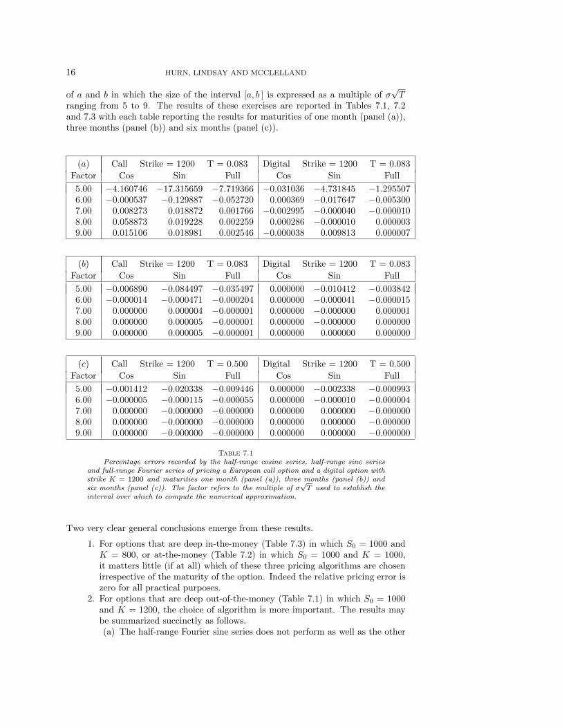
of a and b in which the size of the interval [a, b ] is expressed as a multiple of σ√T
ranging from 5 to 9. The results of these exercises are reported in Tables 7.1, 7.2and 7.3 with each table reporting the results for maturities of one month (panel (a)),three months (panel (b)) and six months (panel (c)).
(a) Call Strike = 1200 T = 0.083 Digital Strike = 1200 T = 0.083
Factor Cos Sin Full Cos Sin Full
5.00 −4.160746 −17.315659 −7.719366 −0.031036 −4.731845 −1.2955076.00 −0.000537 −0.129887 −0.052720 0.000369 −0.017647 −0.0053007.00 0.008273 0.018872 0.001766 −0.002995 −0.000040 −0.0000108.00 0.058873 0.019228 0.002259 0.000286 −0.000010 0.0000039.00 0.015106 0.018981 0.002546 −0.000038 0.009813 0.000007
(b) Call Strike = 1200 T = 0.083 Digital Strike = 1200 T = 0.083
Factor Cos Sin Full Cos Sin Full
5.00 −0.006890 −0.084497 −0.035497 0.000000 −0.010412 −0.0038426.00 −0.000014 −0.000471 −0.000204 0.000000 −0.000041 −0.0000157.00 0.000000 0.000004 −0.000001 0.000000 −0.000000 0.0000018.00 0.000000 0.000005 −0.000001 0.000000 −0.000000 0.0000009.00 0.000000 0.000005 −0.000001 0.000000 0.000000 0.000000
(c) Call Strike = 1200 T = 0.500 Digital Strike = 1200 T = 0.500
Factor Cos Sin Full Cos Sin Full
5.00 −0.001412 −0.020338 −0.009446 0.000000 −0.002338 −0.0009936.00 −0.000005 −0.000115 −0.000055 0.000000 −0.000010 −0.0000047.00 0.000000 −0.000000 −0.000000 0.000000 0.000000 −0.0000008.00 0.000000 −0.000000 −0.000000 0.000000 0.000000 −0.0000009.00 0.000000 −0.000000 −0.000000 0.000000 0.000000 −0.000000
Table 7.1Percentage errors recorded by the half-range cosine series, half-range sine series
and full-range Fourier series of pricing a European call option and a digital option withstrike K = 1200 and maturities one month (panel (a)), three months (panel (b)) andsix months (panel (c)). The factor refers to the multiple of σ
√T used to establish the
interval over which to compute the numerical approximation.
Two very clear general conclusions emerge from these results.
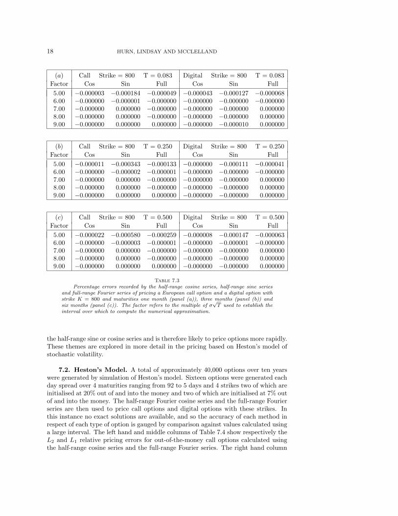
1. For options that are deep in-the-money (Table 7.3) in which S0 = 1000 andK = 800, or at-the-money (Table 7.2) in which S0 = 1000 and K = 1000,it matters little (if at all) which of these three pricing algorithms are chosenirrespective of the maturity of the option. Indeed the relative pricing error iszero for all practical purposes.
2. For options that are deep out-of-the-money (Table 7.1) in which S0 = 1000and K = 1200, the choice of algorithm is more important. The results maybe summarized succinctly as follows.(a) The half-range Fourier sine series does not perform as well as the other
OPTION PRICING 17
(a) Call Strike = 1000 T = 0.083 Digital Strike = 1000 T = 0.083
Factor Cos Sin Full Cos Sin Full
5.00 −0.000044 −0.000313 −0.001045 0.000000 −0.000159 −0.0000436.00 −0.000000 −0.000002 −0.000005 0.000000 −0.000001 −0.0000007.00 0.000000 0.000000 0.000000 0.000000 −0.000000 −0.0000008.00 −0.000000 0.000000 0.000000 0.000000 −0.000000 −0.0000009.00 −0.000000 0.000000 0.000000 0.000000 0.000000 0.000000
(b) Call Strike = 1000 T = 0.250 Digital Strike = 1000 T = 0.250
Factor Cos Sin Full Cos Sin Full
5.00 −0.000063 −0.001375 −0.000547 0.000000 −0.000202 −0.0000746.00 −0.000000 −0.000007 −0.000003 0.000000 −0.000001 −0.0000007.00 0.000000 −0.000000 −0.000000 0.000000 −0.000000 −0.0000008.00 −0.000000 −0.000000 −0.000000 0.000000 −0.000000 −0.0000009.00 −0.000000 −0.000000 −0.000000 0.000000 0.000000 0.000000
(c) Call Strike = 1000 T = 0.500 Digital Strike = 1000 T = 0.500
Factor Cos Sin Full Cos Sin Full
5.00 −0.000116 −0.002208 −0.001059 −0.000000 −0.000254 −0.0001086.00 −0.000000 −0.000012 −0.000006 −0.000000 −0.000001 −0.0000007.00 0.000000 −0.000000 −0.000000 −0.000000 −0.000000 −0.0000008.00 0.000000 −0.000000 0.000000 −0.000000 −0.000000 −0.0000009.00 0.000000 −0.000000 0.000000 −0.000000 −0.000000 −0.000000
Table 7.2Percentage errors recorded by the half-range cosine series, half-range sine series
and full-range Fourier series of pricing a European call option and a digital option withstrike K = 1000 and maturities one month (panel (a)), three months (panel (b)) andsix months (panel (c)). The factor refers to the multiple of σ
√T used to establish the
interval over which to compute the numerical approximation.
two approximations and its use is therefore not recommended.(b) The half-range Fourier cosine series and the full-range Fourier series both
perform relatively well. When the size of the interval of approximationis taken to be a relatively small multiple of σ
√T , namely either 5 or 6,
then the half-range Fourier cosine series performs better that the full-range Fourier series. As the multiple of σ
√T increases and the size
of the interval of approximation becomes larger, the full-range Fourierseries begins to dominate. When the interval of approximation has size10 × σ
√T , then the full-range Fourier series is unambiguously superior
to the half-range Fourier cosine series, particularly for options of shortmaturity.
On the basis of this analysis and on accuracy grounds, it is hard to ignore the claimthat the full-range Fourier series is the algorithm of choice when using Fourier methodsto price options. Moreover, the full-range Fourier series converges faster than either
18 HURN, LINDSAY AND MCCLELLAND
(a) Call Strike = 800 T = 0.083 Digital Strike = 800 T = 0.083
Factor Cos Sin Full Cos Sin Full
5.00 −0.000003 −0.000184 −0.000049 −0.000043 −0.000127 −0.0000686.00 −0.000000 −0.000001 −0.000000 −0.000000 −0.000000 −0.0000007.00 −0.000000 0.000000 −0.000000 −0.000000 −0.000000 0.0000008.00 −0.000000 0.000000 −0.000000 −0.000000 −0.000000 0.0000009.00 −0.000000 0.000000 0.000000 −0.000000 −0.000010 0.000000
(b) Call Strike = 800 T = 0.250 Digital Strike = 800 T = 0.250
Factor Cos Sin Full Cos Sin Full
5.00 −0.000011 −0.000343 −0.000133 −0.000000 −0.000111 −0.0000416.00 −0.000000 −0.000002 −0.000001 −0.000000 −0.000000 −0.0000007.00 −0.000000 0.000000 −0.000000 −0.000000 −0.000000 0.0000008.00 −0.000000 0.000000 −0.000000 −0.000000 −0.000000 0.0000009.00 −0.000000 0.000000 0.000000 −0.000000 −0.000000 0.000000
(c) Call Strike = 800 T = 0.500 Digital Strike = 800 T = 0.500
Factor Cos Sin Full Cos Sin Full
5.00 −0.000022 −0.000580 −0.000259 −0.000008 −0.000147 −0.0000636.00 −0.000000 −0.000003 −0.000001 −0.000000 −0.000001 −0.0000007.00 −0.000000 0.000000 −0.000000 −0.000000 −0.000000 0.0000008.00 −0.000000 0.000000 −0.000000 −0.000000 −0.000000 0.0000009.00 −0.000000 0.000000 0.000000 −0.000000 −0.000000 0.000000
Table 7.3Percentage errors recorded by the half-range cosine series, half-range sine series
and full-range Fourier series of pricing a European call option and a digital option withstrike K = 800 and maturities one month (panel (a)), three months (panel (b)) andsix months (panel (c)). The factor refers to the multiple of σ
√T used to establish the
interval over which to compute the numerical approximation.
the half-range sine or cosine series and is therefore likely to price options more rapidly.These themes are explored in more detail in the pricing based on Heston’s model ofstochastic volatility.
7.2. Heston’s Model. A total of approximately 40,000 options over ten yearswere generated by simulation of Heston’s model. Sixteen options were generated eachday spread over 4 maturities ranging from 92 to 5 days and 4 strikes two of which areinitialised at 20% out of and into the money and two of which are initialised at 7% outof and into the money. The half-range Fourier cosine series and the full-range Fourierseries are then used to price call options and digital options with these strikes. Inthis instance no exact solutions are available, and so the accuracy of each method inrespect of each type of option is gauged by comparison against values calculated usinga large interval. The left hand and middle columns of Table 7.4 show respectively theL2 and L1 relative pricing errors for out-of-the-money call options calculated usingthe half-range cosine series and the full-range Fourier series. The right hand column
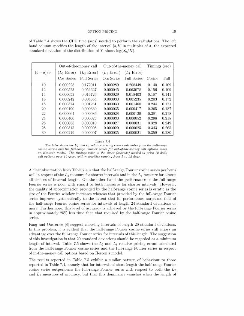
OPTION PRICING 19
of Table 7.4 shows the CPU time (secs) needed to perform the calculations. The lefthand column specifies the length of the interval [a, b ] in multiples of σ, the expectedstandard deviation of the distribution of Y about log(S0/K).
Out-of-the-money call Out-of-the-money call Timings (sec)
(b− a)/σ (L2 Error) (L2 Error) (L1 Error) (L1 Error)
Cos Series Full Series Cos Series Full Series Cosine Full
10 0.000228 0.172011 0.000289 0.208449 0.140 0.10912 0.000523 0.056627 0.000045 0.063078 0.156 0.10914 0.000053 0.016726 0.000029 0.018403 0.187 0.14116 0.000242 0.004654 0.000030 0.005235 0.203 0.17218 0.000374 0.001251 0.000030 0.001468 0.234 0.17120 0.000190 0.000330 0.000035 0.000417 0.265 0.18722 0.000064 0.000086 0.000028 0.000129 0.281 0.21824 0.000460 0.000023 0.000030 0.000052 0.296 0.21826 0.000058 0.000010 0.000027 0.000031 0.328 0.24928 0.000315 0.000008 0.000029 0.000025 0.343 0.26530 0.000219 0.000007 0.000035 0.000021 0.359 0.280
Table 7.4The table shows the L2 and L1 relative pricing errors calculated from the half-range
cosine series and the full-range Fourier series for out-of-the-money call options basedon Heston’s model. The timings refer to the times (seconds) needed to price 12 dailycall options over 10 years with maturities ranging from 5 to 92 days.
A clear observation from Table 7.4 is that the half-range Fourier cosine series performswell in respect of the L2 measure for shorter intervals and in the L1 measure for almostall choices of interval length. On the other hand the performance of the full-rangeFourier series is poor with regard to both measures for shorter intervals. However,the quality of approximation provided by the half-range cosine series is erratic as thesize of the Fourier window increases whereas that provided by the full-range Fourierseries improves systematically to the extent that its performance surpasses that ofthe half-range Fourier cosine series for intervals of length 24 standard deviations ormore. Furthermore, this level of accuracy is achieved by the full-range Fourier seriesin approximately 25% less time than that required by the half-range Fourier cosineseries.
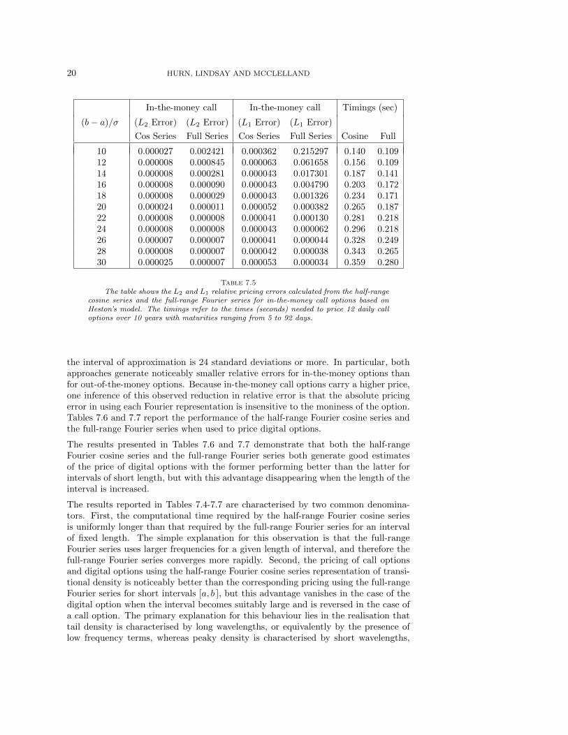
Fang and Oosterlee [8] suggest choosing intervals of length 20 standard deviations.In this problem, it is evident that the half-range Fourier cosine series still enjoys anadvantage over the full-range Fourier series for intervals of this length. The suggestionof this investigation is that 20 standard deviations should be regarded as a minimumlength of interval. Table 7.5 shows the L2 and L1 relative pricing errors calculatedfrom the half-range Fourier cosine series and the full-range Fourier series in respectof in-the-money call options based on Heston’s model.
The results reported in Table 7.5 exhibit a similar pattern of behaviour to thosereported in Table 7.4, namely that for intervals of short length the half-range Fouriercosine series outperforms the full-range Fourier series with respect to both the L2
and L1 measures of accuracy, but that this dominance vanishes when the length of
20 HURN, LINDSAY AND MCCLELLAND
In-the-money call In-the-money call Timings (sec)
(b− a)/σ (L2 Error) (L2 Error) (L1 Error) (L1 Error)
Cos Series Full Series Cos Series Full Series Cosine Full
10 0.000027 0.002421 0.000362 0.215297 0.140 0.10912 0.000008 0.000845 0.000063 0.061658 0.156 0.10914 0.000008 0.000281 0.000043 0.017301 0.187 0.14116 0.000008 0.000090 0.000043 0.004790 0.203 0.17218 0.000008 0.000029 0.000043 0.001326 0.234 0.17120 0.000024 0.000011 0.000052 0.000382 0.265 0.18722 0.000008 0.000008 0.000041 0.000130 0.281 0.21824 0.000008 0.000008 0.000043 0.000062 0.296 0.21826 0.000007 0.000007 0.000041 0.000044 0.328 0.24928 0.000008 0.000007 0.000042 0.000038 0.343 0.26530 0.000025 0.000007 0.000053 0.000034 0.359 0.280
Table 7.5The table shows the L2 and L1 relative pricing errors calculated from the half-range
cosine series and the full-range Fourier series for in-the-money call options based onHeston’s model. The timings refer to the times (seconds) needed to price 12 daily calloptions over 10 years with maturities ranging from 5 to 92 days.
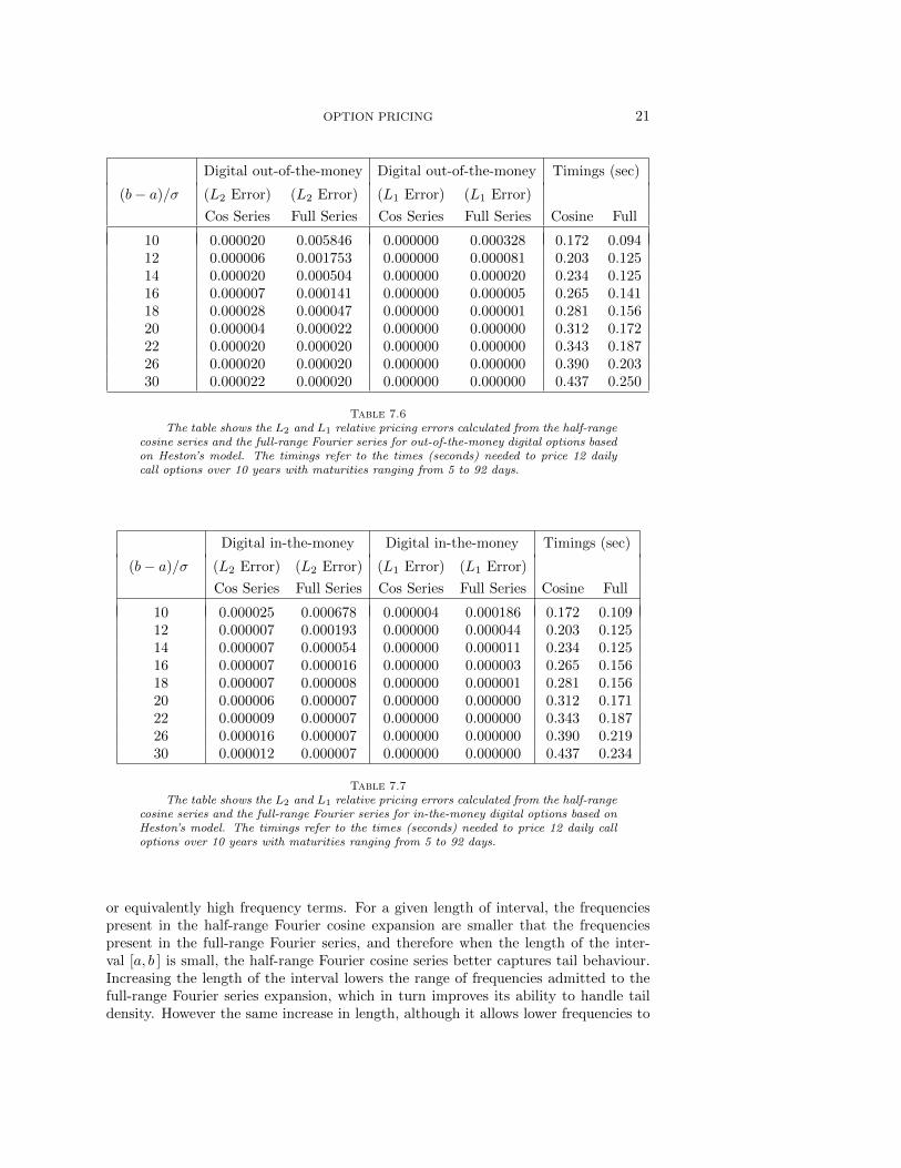
the interval of approximation is 24 standard deviations or more. In particular, bothapproaches generate noticeably smaller relative errors for in-the-money options thanfor out-of-the-money options. Because in-the-money call options carry a higher price,one inference of this observed reduction in relative error is that the absolute pricingerror in using each Fourier representation is insensitive to the moniness of the option.Tables 7.6 and 7.7 report the performance of the half-range Fourier cosine series andthe full-range Fourier series when used to price digital options.
The results presented in Tables 7.6 and 7.7 demonstrate that both the half-rangeFourier cosine series and the full-range Fourier series both generate good estimatesof the price of digital options with the former performing better than the latter forintervals of short length, but with this advantage disappearing when the length of theinterval is increased.
The results reported in Tables 7.4-7.7 are characterised by two common denomina-tors. First, the computational time required by the half-range Fourier cosine seriesis uniformly longer than that required by the full-range Fourier series for an intervalof fixed length. The simple explanation for this observation is that the full-rangeFourier series uses larger frequencies for a given length of interval, and therefore thefull-range Fourier series converges more rapidly. Second, the pricing of call optionsand digital options using the half-range Fourier cosine series representation of transi-tional density is noticeably better than the corresponding pricing using the full-rangeFourier series for short intervals [a, b ], but this advantage vanishes in the case of thedigital option when the interval becomes suitably large and is reversed in the case ofa call option. The primary explanation for this behaviour lies in the realisation thattail density is characterised by long wavelengths, or equivalently by the presence oflow frequency terms, whereas peaky density is characterised by short wavelengths,
OPTION PRICING 21
Digital out-of-the-money Digital out-of-the-money Timings (sec)
(b− a)/σ (L2 Error) (L2 Error) (L1 Error) (L1 Error)
Cos Series Full Series Cos Series Full Series Cosine Full
10 0.000020 0.005846 0.000000 0.000328 0.172 0.09412 0.000006 0.001753 0.000000 0.000081 0.203 0.12514 0.000020 0.000504 0.000000 0.000020 0.234 0.12516 0.000007 0.000141 0.000000 0.000005 0.265 0.14118 0.000028 0.000047 0.000000 0.000001 0.281 0.15620 0.000004 0.000022 0.000000 0.000000 0.312 0.17222 0.000020 0.000020 0.000000 0.000000 0.343 0.18726 0.000020 0.000020 0.000000 0.000000 0.390 0.20330 0.000022 0.000020 0.000000 0.000000 0.437 0.250
Table 7.6The table shows the L2 and L1 relative pricing errors calculated from the half-range
cosine series and the full-range Fourier series for out-of-the-money digital options basedon Heston’s model. The timings refer to the times (seconds) needed to price 12 dailycall options over 10 years with maturities ranging from 5 to 92 days.
Digital in-the-money Digital in-the-money Timings (sec)
(b− a)/σ (L2 Error) (L2 Error) (L1 Error) (L1 Error)
Cos Series Full Series Cos Series Full Series Cosine Full
10 0.000025 0.000678 0.000004 0.000186 0.172 0.10912 0.000007 0.000193 0.000000 0.000044 0.203 0.12514 0.000007 0.000054 0.000000 0.000011 0.234 0.12516 0.000007 0.000016 0.000000 0.000003 0.265 0.15618 0.000007 0.000008 0.000000 0.000001 0.281 0.15620 0.000006 0.000007 0.000000 0.000000 0.312 0.17122 0.000009 0.000007 0.000000 0.000000 0.343 0.18726 0.000016 0.000007 0.000000 0.000000 0.390 0.21930 0.000012 0.000007 0.000000 0.000000 0.437 0.234
Table 7.7The table shows the L2 and L1 relative pricing errors calculated from the half-range
cosine series and the full-range Fourier series for in-the-money digital options based onHeston’s model. The timings refer to the times (seconds) needed to price 12 daily calloptions over 10 years with maturities ranging from 5 to 92 days.
or equivalently high frequency terms. For a given length of interval, the frequenciespresent in the half-range Fourier cosine expansion are smaller that the frequenciespresent in the full-range Fourier series, and therefore when the length of the inter-val [a, b ] is small, the half-range Fourier cosine series better captures tail behaviour.Increasing the length of the interval lowers the range of frequencies admitted to thefull-range Fourier series expansion, which in turn improves its ability to handle taildensity. However the same increase in length, although it allows lower frequencies to
22 HURN, LINDSAY AND MCCLELLAND
enter the half-range Fourier cosine series representation of transitional density, theirpresence will have an impact only if there is significant tail density to be characterisedby these new frequencies. On the other hand, the half-range Fourier cosine series hasthe drawback that the (periodic) function it represents is not differentiable at x = a incontrast to the behaviour of the function represented by the full-range Fourier series.
8. Conclusion. One clear conclusion from these calculations is that the half-range Fourier cosine series and the full-range Fourier series perform uniformly betterthat the half-range Fourier sine series. The half-range Fourier cosine series and thefull-range Fourier series both perform with credit. When the length of the interval[a, b ] is relatively small, say ten or so standard deviations, it is clear that the half-rangeFourier cosine series outperforms the full-range Fourier series over the same interval.On the other hand for intervals of larger length the full-range Fourier series is at leastas good as the half-range Fourier cosine series, and outperforms the latter in pricingout-of-the-money call options, in particular, with maturities of three months or less.In fact the full-range Fourier series outperforms the half-range Fourier cosine seriesin all circumstances provided the interval [a, b ] is suitably large, although the effectis so small as not to be significant in practice. The explanation for this behaviourlies in the fact that the half-range Fourier cosine series, although not representing adifferentiable function, nevertheless always uses a lower spectrum of frequencies thanthe full-range Fourier series and therefore enjoys an initial advantage in describingtail density. As the interval length is increased, this advantage vanishes. On theother hand the larger spectrum of the full-range Fourier series guarantees more rapidconvergence. Of course, timing issues may not be important if small numbers of modelcall prices are to be calculated, but when each and every evaluation of the likelihoodfunction requires in excess of one billion calculations of the model call price as occurswith a particle filtering algorithm, timing issues are now significant once adequatenumerical accuracy is assured.
REFERENCES
[1] F. Black and M. Scholes, The pricing of options and corporate liabilities, Journal of PoliticalEconomy, 81 (1973), pp. 637 – 654.
[2] S. Borak, K. Detlefsen, and W. Hardle, FFT based option pricing, SFB Discussion Paper649, (2005).
[3] M. Broadie, M. Chernov, and M. Johannes, Model specification and risk premia: Evidencefrom futures options, Journal of Finance, 62 (2007), pp. 1453–1490.
[4] P.P. Carr and D.B. Madan, Option evaluation using the Fast Fourier Transform, Journalof Computational Finance, 2 (1999), pp. 61 – 73.
[5] P. Christoffersen, K. Jacobs, and K. Mimouni, Volatility dynamics for the s&p500: Evi-dence from realized volatility, daily returns and option prices, Review of Financial Studies,23 (2010), pp. 3141–3189.
[6] G. Durham and J. Geweke, Massively parallel sequential Monte Carlo for bayesian inference,Unpublished manuscript, (2011).
[7] , Adaptive sequential posterior simulators for massively parallel computing environments,Unpublished manuscript, (2012).
[8] F. Fang and C.W. Oosterlee, A novel pricing method for european options based on fourier-cosine series expansions, Working Paper, Munich Personal RePEc Archive, (2008).
[9] S.L. Heston, A closed-form solution for options with stochastic volatility with applications tobond and currency options, Review of Financial Studies, (1993), pp. 327–343.
[10] A.S. Hurn, K.A. Lindsay, and A.J. McClelland, Estimating the parameters of stochasticvolatility models using option price data, Unpublished Working Paper, NCER, (2012).
[11] M.S. Johannes, N.G. Polson, and J.R. Stroud, Optimal filtering of jump diffusions: Ex-tracting latent states from asset prices, Review of Financial Studies, 22 (2009), pp. 2759 –

OPTION PRICING 23
2799.[12] Y.K. Kwok, K.S. Leung, and H.Y. Wong, Efficient options pricing using the Fast Fourier
Transform, in Handbook of Computational Finance, J.C. Duan, ed., Springer, 2012.[13] R. Lord, F. Fang, F. Bervoets, and C.W. Oosterlee, A fast and accurate FFT-based
methodology for pricing early-exercise options under levy processes, SIAM Journal of Sci-entific Computing, 20 (2007), pp. 1678 – 1705.
[14] B. Zhang, L.A. Grzelak, and C.W. Oosterlee, Efficient pricing of commodity options withearly-exercise under the Ornstein-Uhlenbeck process, Applied Numerical Mathematics, 62(2012), pp. 91 – 111.