On the Effects of Surface Roughness on Boundary Layer Transition

Meelan Choudhari, Fei Li, Chau-Lyan ChangNASA Langley Research Center, Hampton, VA 23681

Jack EdwardsNorth Carolina State University, Raleigh, NC 27695

Surface roughness can influence laminar-turbulent transition in many different ways.This paper outlines selected analyses performed at the NASA Langley Research Center,ranging in speed from subsonic to hypersonic Mach numbers and highlighting the beneficialas well as adverse roles of the surface roughness in technological applications. The firsttheme pertains to boundary-layer tripping on the forebody of a hypersonic airbreathingconfiguration via a spanwise periodic array of trip elements, with the goal of understandingthe physical mechanisms underlying roughness-induced transition in a high-speed boundarylayer. The effect of an isolated, finite amplitude roughness element on a supersonicboundary layer is considered next. The other set of flow configurations examined hereincorresponds to roughness based laminar flow control in subsonic and supersonic swept wingboundary layers. A common theme to all of the above configurations is the need to applyhigher fidelity, physics based techniques to develop reliable predictions of roughness effectson laminar-turbulent transition.

I. INTRODUCTION

Surface roughness is known to have a substantial impact on boundary-layer transition and, hence, on theaerodynamic and/or aerothermodynamic predictions for flight vehicles across a wide range of Mach numbers. Smallamplitude roughness over the appropriate range of surface locations may serve as a catalyst during the excitation oftraveling wave instabilities due to free-stream unsteadiness, or act as a direct source of stationary vortex instabilitiessuch as Gortler vortices and stationary crossflow modes. A striking example of the effect of roughness-inducedreceptivity on transition has been documented in [1], where transition was noted to move from between 25 to 30percent chord to 80 percent chord when the painted leading edge was polished so as to reduce the roughnessamplitude from 1.0 gm rms (3.8 µm average peak-to-peak) to 0.3 µm rms (2.2 gm average peak-to-peak). A recentlyproposed concept for transition control over swept aerodynamic surfaces involves the use of distributed roughnesselements (DREs) near the leading edge [1, 2]. The DREs excite subdominant stationary crossflow modes that arenot strong enough to cause transition on their own but can modify the underlying basic state so as to reduce thegrowth of the linearly most unstable crossflow modes.

Roughness at intermediate heights can further lead to a substantial modification of the underlying boundary layerand also scatter any incoming instability waves, so as to exert an overall impact on the growth characteristics of theboundary layer perturbations (see, e.g., [3]). A roughness strip producing a sufficiently large perturbation in surfaceheight is often employed as a means to induce earlier transition in a laminar boundary layer. In certain other cases,the presence of unavoidable variations in surface geometry leads to unintended tripping of the boundary layer. Thedetailed physical mechanisms associated with roughness-induced tripping are not fully understood yet. Inincompressible boundary layers, however, the earlier onset of transition behind discrete roughness elements may belinked to a spontaneous onset of vortex shedding behind the element [4]. On the other hand, there is reason tobelieve that the mechanism of laminar-turbulent transition due to distributed surface roughness may be related to atransient but large growth of linearly stable perturbations excited by the surface roughness [5]. For additionalinformation pertaining to roughness effects on transition, the reader is referred to [6, 7].

This paper summarizes a select set of recent investigations involving the computations of roughness effects onboundary layer transition. For more complete descriptions of these studies, the reader is directed to Refs. [8–11].Boundary-layer tripping mechanisms associated with spanwise periodic and isolated roughness elements in a high-speed boundary layer are discussed in Section 2. Section 3 is devoted to high fidelity transition analyses for thedelay of crossflow transition in swept wing boundary layers using distributed roughness elements (DREs) near theleading edge. Because the transition delay via DREs is achieved via nonlinear effects associated with artificially

https://ntrs.nasa.gov/search.jsp?R=20090033115 2018-08-08T04:03:52+00:00Z

seeded modes, laminar flow design based on this technique intrinsically demands integrated prediction methods thatgo beyond the linear stability correlations typically employed in the context of other laminar flow controltechniques. With that in mind, this paper attempts to include the linear and nonlinear growth of primary crossflowmodes along with the linear amplification of high-frequency secondary instabilities towards more holisticpredictions of the transition behavior. Section 3 describes the application of an N-factor criterion based onsecondary instabilities of stationary crossflow modes to realistic flow configurations designed for DREs. Theseexamples highlight the critical need to achieve a balance between sufficiently large and not-too-large control inputsfor the successful implementation of the DRE technique in higher Reynolds number flows, as well as illustratinghow such balance might be achieved via higher fidelity analyses techniques. Finally, some of the remainingchallenges in applying such techniques are also pointed out.

II. Roughness-Induced Tripping in High-Speed Boundary Layers

A. Spanwise Periodic Trip Array on Hyper -X ForebodyThe computations described herein model the Hyper-X Mach 6 flow configuration from Ref. [12] at a nominal unitReynolds number of Re = 2.2 x 10 6/ft. The 0.333 scale forebody model tested in these experiments is 28 incheslong, with a trip insert location at 7.4 inches from the leading edge. The model geometry consists of a roundedleading edge with a nose radius of 0.01 inches, followed by three flat ramps providing discrete, sequential, non-isentropic flow compressions ahead of the engine. At the nominal angle of attack equal to 2 degrees, the localcompression angles for the three ramps correspond to 4.5, 5.5, and 3 degrees, respectively. The first compressioncorner (between ramps 1 and 2) is located at 12.4 inches, and the second corner at 17.7 inches. Of the various tripconfigurations tested in the experiment, trip configuration 2c (Fig. 1) was identified as providing the bestcombination of tripping effectiveness and reduced axial vorticity within the turbulent flow approaching the inlet.The results presented herein correspond to a trip spacing of S = 0.081” and a peak height of h = 0.060”. The lattertrip height was sufficient to promote transition fairly close to the trip location in the experiment. Although the tripspacing for the computations described herein is smaller than the 0.12” spacing in Ref. [12], a comparison ofcomputations for both trip spacing cases showed similar results as discussed in Ref. [8].

To obtain the mean-flow solution in the presence ofthe trip array, the compressible Navier-Stokesequations are solved using either global or local timestepping in conjunction with an implicit technique and4th order discretization of advection terms. Theimmersed boundary (IB) technique [13] is used tosimulate the effects of the trip array on the surroundingflow.

Trip 2c (Ramp Trip) The spanwise varying boundary layer displacement

Figure 1. Schematic of trip configuration 2c due to the trip elements results in the formation of

(reproduced from Ref. [8]). Here, δ denotes the strong streamwise streaks in the wake of the trip array

array spacing and h represents the maximum (Fig. 2). The velocity contours at several streamwise

height of a trip element. stations reveal that the streaks would persist for longdistances over the forebody surface if the boundary-

layer flow were to remain laminar throughout that region. The presence of longitudinal streaks behind the trip arraywas also noted in the conventional facility experiments by Berry et al. [14] as well as in the more recentmeasurements by Borg et al. [10] on the X-51A model, a configuration similar to Hyper-X, which was tested underboth quiet and noisy conditions. The computations also indicate a rapid increase in streak amplitude across thecompression corner (Fig. 3), a finding that is in qualitative agreement with the measurements in [14].

The stability characteristics of the roughness wake are examined next, with the goal of understanding whether theonset of transition behind the trip array may be related to the amplification of instability modes supported by theabovementioned streaks. Since the spanwise and wall-normal length scales of these streaks are comparable witheach other, the modified boundary-layer flow has a strongly inhomogeneous character in both y and z directions.Therefore, its stability characteristics are more appropriately studied by solving a 2D eigenvalue problem, ratherthan using the conventional linear stability analysis, which is based on the assumption of basic state inhomogeneityalong just the surface normal direction.

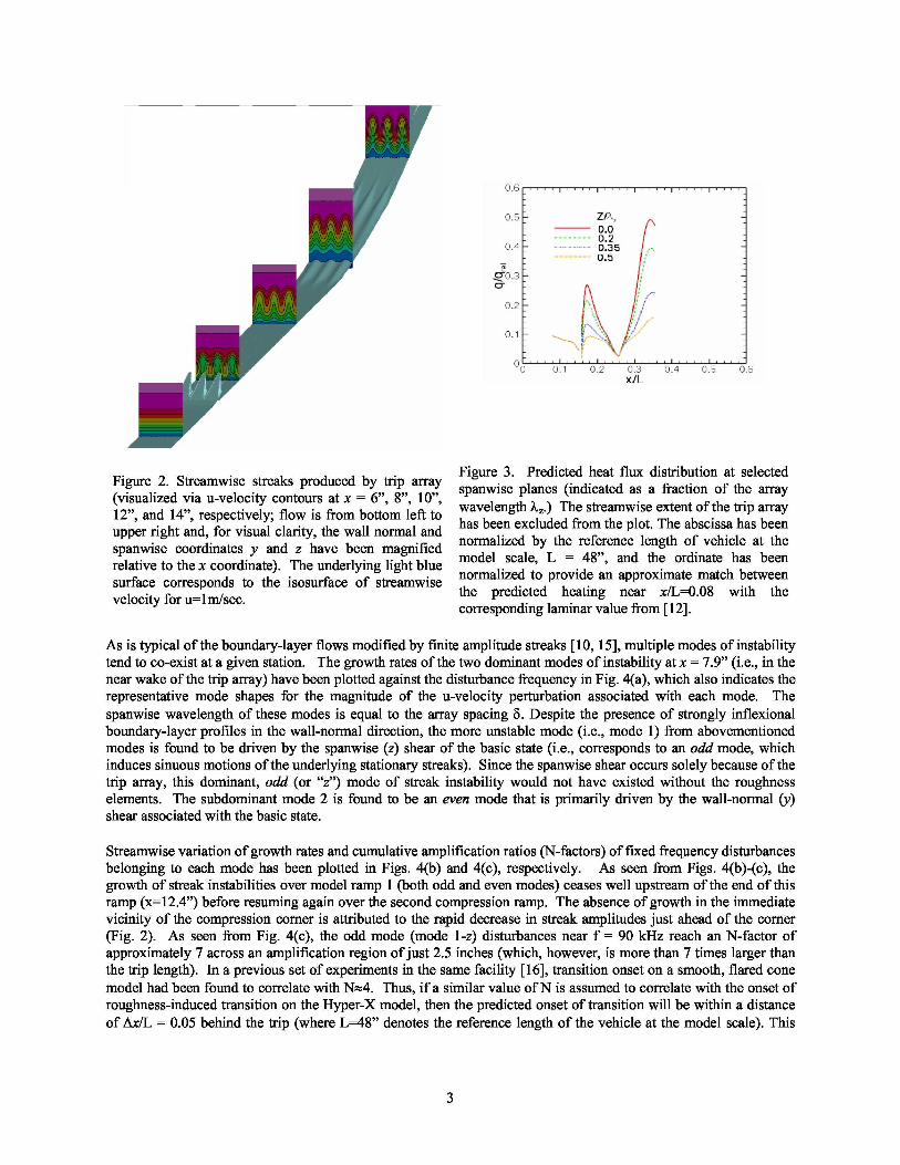
Figure 2. Streamwise streaks produced by trip array(visualized via u-velocity contours at x = 6”, 8”, 10”,12”, and 14”, respectively; flow is from bottom left toupper right and, for visual clarity, the wall normal andspanwise coordinates y and z have been magnifiedrelative to the x coordinate). The underlying light bluesurface corresponds to the isosurface of streamwisevelocity for u=1m/sec.

Figure 3. Predicted heat flux distribution at selectedspanwise planes (indicated as a fraction of the arraywavelength λz.) The streamwise extent of the trip arrayhas been excluded from the plot. The abscissa has beennormalized by the reference length of vehicle at themodel scale, L = 48”, and the ordinate has beennormalized to provide an approximate match betweenthe predicted heating near x/L=0.08 with thecorresponding laminar value from [12].

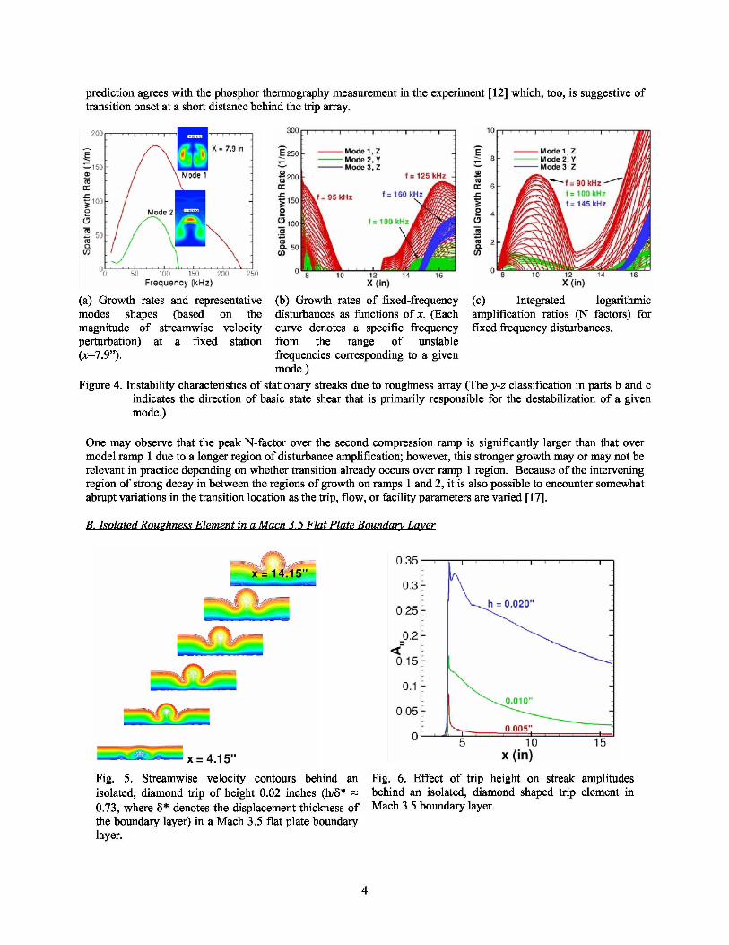
As is typical of the boundary-layer flows modified by finite amplitude streaks [10, 15], multiple modes of instabilitytend to co-exist at a given station. The growth rates of the two dominant modes of instability at x = 7.9” (i.e., in thenear wake of the trip array) have been plotted against the disturbance frequency in Fig. 4(a), which also indicates therepresentative mode shapes for the magnitude of the u-velocity perturbation associated with each mode. Thespanwise wavelength of these modes is equal to the array spacing S. Despite the presence of strongly inflexionalboundary-layer profiles in the wall-normal direction, the more unstable mode (i.e., mode 1) from abovementionedmodes is found to be driven by the spanwise ( z) shear of the basic state (i.e., corresponds to an odd mode, whichinduces sinuous motions of the underlying stationary streaks). Since the spanwise shear occurs solely because of thetrip array, this dominant, odd (or “z”) mode of streak instability would not have existed without the roughnesselements. The subdominant mode 2 is found to be an even mode that is primarily driven by the wall-normal ( y)shear associated with the basic state.

Streamwise variation of growth rates and cumulative amplification ratios (N-factors) of fixed frequency disturbancesbelonging to each mode has been plotted in Figs. 4(b) and 4(c), respectively. As seen from Figs. 4(b)-(c), thegrowth of streak instabilities over model ramp 1 (both odd and even modes) ceases well upstream of the end of thisramp (x=12.4”) before resuming again over the second compression ramp. The absence of growth in the immediatevicinity of the compression corner is attributed to the rapid decrease in streak amplitudes just ahead of the corner(Fig. 2). As seen from Fig. 4(c), the odd mode (mode 1- z) disturbances near f = 90 kHz reach an N-factor ofapproximately 7 across an amplification region of just 2.5 inches (which, however, is more than 7 times larger thanthe trip length). In a previous set of experiments in the same facility [16], transition onset on a smooth, flared conemodel had been found to correlate with N=4. Thus, if a similar value of N is assumed to correlate with the onset ofroughness-induced transition on the Hyper-X model, then the predicted onset of transition will be within a distanceof Ox/L = 0.05 behind the trip (where L=48” denotes the reference length of the vehicle at the model scale). This

prediction agrees with the phosphor thermography measurement in the experiment [12] which, too, is suggestive oftransition onset at a short distance behind the trip array.

(a) Growth rates and representativemodes shapes (based on themagnitude of streamwise velocityperturbation) at a fixed station(x=7.9”).

(b) Growth rates of fixed-frequencydisturbances as functions of x. (Eachcurve denotes a specific frequencyfrom the range of unstablefrequencies corresponding to a givenmode.)

(c) Integrated logarithmicamplification ratios (N factors) forfixed frequency disturbances.

Figure 4. Instability characteristics of stationary streaks due to roughness array (The y-z classification in parts b and cindicates the direction of basic state shear that is primarily responsible for the destabilization of a givenmode.)

One may observe that the peak N-factor over the second compression ramp is significantly larger than that overmodel ramp 1 due to a longer region of disturbance amplification; however, this stronger growth may or may not berelevant in practice depending on whether transition already occurs over ramp 1 region. Because of the interveningregion of strong decay in between the regions of growth on ramps 1 and 2, it is also possible to encounter somewhatabrupt variations in the transition location as the trip, flow, or facility parameters are varied [17].

B. Isolated Roughness Element in a Mach 3.5 Flat Plate Boundar y Layer

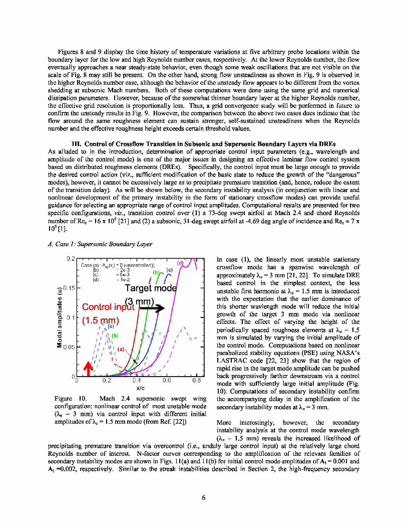
Fig. 5. Streamwise velocity contours behind anisolated, diamond trip of height 0.02 inches (h/S*0.73, where S* denotes the displacement thickness ofthe boundary layer) in a Mach 3.5 flat plate boundarylayer.

Fig. 6. Effect of trip height on streak amplitudesbehind an isolated, diamond shaped trip element inMach 3.5 boundary layer.

To further understand the effect of the compression corner, the case of an isolated trip without the destabilizinginfluence of a compression corner is examined next. Ccomputations similar to those for the Hyper-X trip array wereperformed for an isolated diamond trip mounted on a flat plate at zero incidence to the incoming free stream (Fig. 5).The flow conditions for these computations (M=3.5, Re=3x10 6/ft, T=90.2 deg K, width of each face of diamond trip= 0.05 inches) were chosen to be relevant to a planned experiment in the Supersonic Low Disturbance Tunnel atNASA Langley Research Center.

As shown in Fig. 6, streak amplitudes for the flat plate case decay nearly monotonically with distance from the trip(or the trip array), in contrast to the case of Hyper-X like compression surfaces where the rapid increase in streakstrength near the compression corner helped sustain the strong streak amplitudes over large distances (Fig. 3). Fig. 6also shows that the streak amplitudes have a strongly nonlinear dependence on the roughness height, not unlike thecase of roughness-induced streaks in low-speed flows [18, 19]. Thus, no streak instabilities of the type discussedearlier are expected to exist behind the shallowest trip of height 0.005”, whereas sufficiently strong wake instabilityis predicted to occur behind the trip element with the largest height.

c. Parameter Study for Isolated Roughness Element in a Flat Plate Boundar y LayerAdditional computations have been carried out for both 2D and 3D roughness elements at other Mach numbersusing the unstructured grid code EZ4D [9]. The 2D computations at subsonic Mach numbers reveal the presence ofvortex shedding at sufficiently large roughness heights, which is suggestive of an absolute instability in the region ofseparation near the roughness element. The vortex shedding process weakens with increasing subsonic Machnumber and no visibly obvious shedding was observed in the context of 2D computations at supersonic Machnumbers. Of course, the dominant instability modes at supersonic Mach numbers are known to be three-dimensional. Yet, as described below, no strong shedding was noted even in 3D, supersonic computations atroughness height Reynolds numbers that would have resulted in shedding in low-speed boundary layers.

Figure 7 shows the numerical Schlieren picture for a Mach 9.65 flow impinging on a flat plate with a cylindricalroughness element at approximately 3 inches from the sharp leading edge. The free-stream and wall temperaturesare 53.3 K and 308 K, respectively. The plate is at an angle of attack equal to 20 deg, and the post shock Machnumber is 4.16. The diameter and height of the cylindrical roughness element are equal to 4 mm and 2 mm,respectively. Time accurate Navier-Stokes computations were performed for two different stagnation pressures atwhich experiments have been performed at NASA Langley [20]. The corresponding Reynolds numbers based onpost-shock unit Reynolds number and the height of the roughness element are approximately 6800 and 14300,respectively. Using the Sutherland law for viscosity, the roughness height to the boundary layer thickness ratio isnearly 1.3 and 2.8, respectively.

Figure 7. Numerical Schlierenpicture at the symmetry plane andsurface pressure contours for aMach 9.65 flow over a cylindricalroughness element.

Figure 8. Time history oftemperature variation at five arbitraryprobe locations around the cylindricalroughness element at the lowerReynolds number of 6800 (Bothabscissa and ordinate are suitablynondimensionalized.)

Figure 9. Time history of temperaturevariation at five different probelocations around the cylindricalroughness element at the higherReynolds number of 14300.

Figures 8 and 9 display the time history of temperature variations at five arbitrary probe locations within theboundary layer for the low and high Reynolds number cases, respectively. At the lower Reynolds number, the floweventually approaches a near steady-state behavior, even though some weak oscillations that are not visible on thescale of Fig. 8 may still be present. On the other hand, strong flow unsteadiness as shown in Fig. 9 is observed inthe higher Reynolds number case, although the behavior of the unsteady flow appears to be different from the vortexshedding at subsonic Mach numbers. Both of these computations were done using the same grid and numericaldissipation parameters. However, because of the somewhat thinner boundary layer at the higher Reynolds number,the effective grid resolution is proportionally less. Thus, a grid convergence study will be performed in future toconfirm the unsteady results in Fig. 9. However, the comparison between the above two cases does indicate that theflow around the same roughness element can sustain stronger, self-sustained unsteadiness when the Reynoldsnumber and the effective roughness height exceeds certain threshold values.

III. Control of Crossflow Transition in Subsonic and Supersonic Boundary Layers via DREsAs alluded to in the introduction, determination of appropriate control input parameters (e.g., wavelength andamplitude of the control mode) is one of the major issues in designing an effective laminar flow control systembased on distributed roughness elements (DREs). Specifically, the control input must be large enough to providethe desired control action (viz., sufficient modification of the basic state to reduce the growth of the “dangerous”modes), however, it cannot be excessively large as to precipitate premature transition (and, hence, reduce the extentof the transition delay). As will be shown below, the secondary instability analysis (in conjunction with linear andnonlinear development of the primary instability in the form of stationary crossflow modes) can provide usefulguidance for selecting an appropriate range of control input amplitudes. Computational results are presented for twospecific configurations, viz., transition control over (1) a 73-deg swept airfoil at Mach 2.4 and chord Reynoldsnumber of Re c = 16 x 106 [21] and (2) a subsonic, 31-deg swept airfoil at -4.69 deg angle of incidence and Re c = 7 x106 [1].

Figure 10. Mach 2.4 supersonic swept wingconfiguration: nonlinear control of most unstable mode(Ȝz = 3 mm) via control input with different initial

In case (1), the linearly most unstable stationarycrossflow mode has a spanwise wavelength ofapproximately X,z = 3 mm [21, 22]. To simulate DREbased control in the simplest context, the lessunstable first harmonic at X,z = 1.5 mm is introducedwith the expectation that the earlier dominance ofthis shorter wavlength mode will reduce the initialgrowth of the target 3 mm mode via nonlineareffects. The effect of varying the height of theperiodically spaced roughness elements at X,z = 1.5mm is simulated by varying the initial amplitude ofthe control mode. Computations based on nonlinearparabolized stability equations (PSE) using NASA’sLASTRAC code [22, 23] show that the region ofrapid rise in the target mode amplitude can be pushedback progressively farther downstream via a controlmode with sufficiently large initial amplitude (Fig.10). Computations of secondary instability confirmthe accompanying delay in the amplification of thesecondary instability modes at X,z = 3 mm.

A. Case 1: Supersonic Boundary Layer

l asea1 ; 0 1x1,1 1lC'11L;11G611tudedl]

1V-2' 7^'(Target Mod

Control inp JtM)

(1.5 MM)

amplitudes of Ȝz = 1.5 mm mode (from Ref. [22]) More interestingly, however, the secondaryinstability analysis at the control mode wavelength(X,z = 1.5 mm) reveals the increased likelihood of

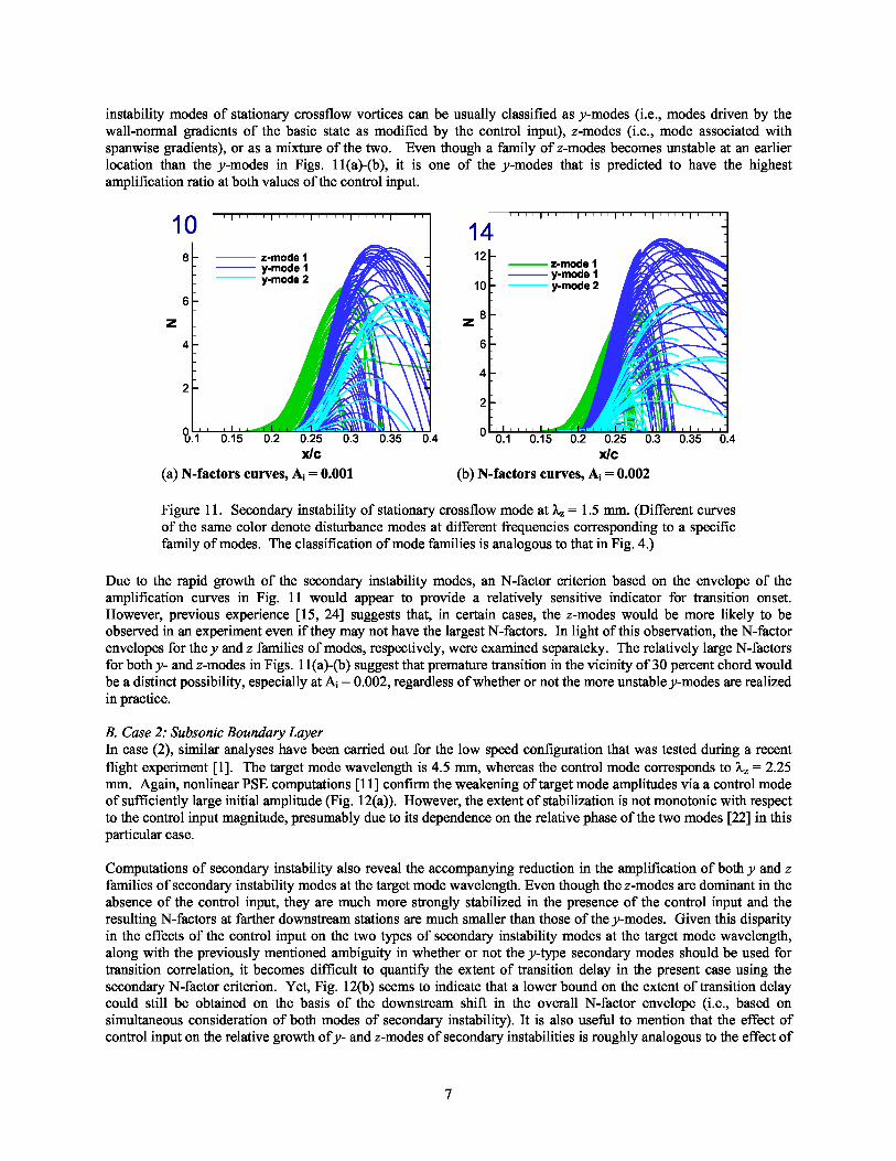
precipitating premature transition via overcontrol (i.e., unduly large control input) at the relatively large chordReynolds number of interest. N-factor curves corresponding to the amplification of the relevant families ofsecondary instability modes are shown in Figs. 1 1 (a) and 1 1 (b) for initial control mode amplitudes of Ai = 0.001 andAi =0.002, respectively. Similar to the streak instabilities described in Section 2, the high-frequency secondary

1412

z-mode 1y-mode 1

10 y-mode 2

Z 8

X/cX/c

10

10

instability modes of stationary crossflow vortices can be usually classified as y-modes (i.e., modes driven by thewall-normal gradients of the basic state as modified by the control input), z-modes (i.e., mode associated withspanwise gradients), or as a mixture of the two. Even though a family of z-modes becomes unstable at an earlierlocation than the y-modes in Figs. 11(a)-(b), it is one of the y-modes that is predicted to have the highestamplification ratio at both values of the control input.

(a) N-factors curves, A; = 0.001

(b) N-factors curves, A; = 0.002

Figure 11. Secondary instability of stationary crossflow mode at ^z = 1.5 mm. (Different curvesof the same color denote disturbance modes at different frequencies corresponding to a specificfamily of modes. The classification of mode families is analogous to that in Fig. 4.)

Due to the rapid growth of the secondary instability modes, an N-factor criterion based on the envelope of theamplification curves in Fig. 11 would appear to provide a relatively sensitive indicator for transition onset.However, previous experience [15, 24] suggests that, in certain cases, the z-modes would be more likely to beobserved in an experiment even if they may not have the largest N-factors. In light of this observation, the N-factorenvelopes for the y and z families of modes, respectively, were examined separateky. The relatively large N-factorsfor both y- and z-modes in Figs. 1 1 (a)-(b) suggest that premature transition in the vicinity of 30 percent chord wouldbe a distinct possibility, especially at A i = 0.002, regardless of whether or not the more unstable y-modes are realizedin practice.

B. Case 2: Subsonic Boundary LayerIn case (2), similar analyses have been carried out for the low speed configuration that was tested during a recentflight experiment [1]. The target mode wavelength is 4.5 mm, whereas the control mode corresponds to λz = 2.25mm. Again, nonlinear PSE computations [11] confirm the weakening of target mode amplitudes via a control modeof sufficiently large initial amplitude (Fig. 12(a)). However, the extent of stabilization is not monotonic with respectto the control input magnitude, presumably due to its dependence on the relative phase of the two modes [22] in thisparticular case.

Computations of secondary instability also reveal the accompanying reduction in the amplification of both y and zfamilies of secondary instability modes at the target mode wavelength. Even though the z-modes are dominant in theabsence of the control input, they are much more strongly stabilized in the presence of the control input and theresulting N-factors at farther downstream stations are much smaller than those of the y-modes. Given this disparityin the effects of the control input on the two types of secondary instability modes at the target mode wavelength,along with the previously mentioned ambiguity in whether or not the y-type secondary modes should be used fortransition correlation, it becomes difficult to quantify the extent of transition delay in the present case using thesecondary N-factor criterion. Yet, Fig. 12(b) seems to indicate that a lower bound on the extent of transition delaycould still be obtained on the basis of the downstream shift in the overall N-factor envelope (i.e., based onsimultaneous consideration of both modes of secondary instability). It is also useful to mention that the effect ofcontrol input on the relative growth of y- and z-modes of secondary instabilities is roughly analogous to the effect of

lowering the initial amplitude of the target mode in the no-control case. In the course of engineering analyses, itmight be possible to exploit this similarity by limiting the relatively expensive secondary instability calculations to abasic state that is based on the nonlinear evolution of the target mode alone at various initial amplitudes (i.e., withzero control input).

Figure 12(a) Modal amplitude evolution of linearlymost unstable stationary crossflow mode (λz = 4.5mm) in the presence of control input at λz = 2.25 mm

The uncertainty related to whether both y- and z-modes of secondary instability or just the z-modesshould be used for N-factor correlation also has animpact on predicting the potential for overcontrol incase (2). Specifically, secondary instability analysisat the control mode wavelength indicates that the z-modes at λz = 2.25 mm have rather small N-factorsat both A i = 0.005 and 0.0 1, but that the y-modes canreach N-factor values exceeding 9 for the largercontrol input. Thus, whether or not prematuretransition due to unduly large control input willoccur in that case would depend on the realizabilityand receptivity characteristics of the y-modes [25].The latter issues cannot be directly addressed in thecourse of the flight experiment [1]; however,measurements of the crossflow disturbanceamplitudes, together with simultaneousmeasurements of transition onset could providesufficient data to help reduce the associateduncertainty in applying a secondary N-factorcriterion to other similar configurations.

(b) N-factor envelopes for dominant y- and z-mode (c) Linear growth of X = 4.5 mm stationarysecondary instabilities with λz = 4.5 mm for initial crossflow mode with and without mean flowcontrol mode amplitudes of A i = 0, 0.005, and 0.01. correction due to control input (Initial amplitude

Ai = 0.01)Figure 12. DRE based laminar flow control on the subsonic, SWIFT flight configuration [1].

Finally, to explore a computationally easier alternative to secondary instability analysis in the context of DREs, Fig.12(c) examines the linear stability of the spanwise averaged flow in the presence of the nonlinear distortion due tothe control input. Specifically, it compares the N-factor values for the target mode as predicted via linear instabilityanalysis of the spanwise averaged mean flow without and with the control input. The figure shows that the basicstate modification due to the control mode results in a significant reduction in the peak N-factor relative to the

8

uncontrolled case (AN = 3.2 near x/c=0.6). However, additional work is necessary to establish whether and howsuch simplified analysis may be applied towards the design of DREs.

IV. SUMMARY

By applying artificial roughness elements, boundary layer transition can be either hastened or delayed, depending onthe specific requirements for flow control. In the case of boundary layer tripping over a compression surface aheadof the engine inlet on a hypersonic air-breathing configuration, roughness elements generate stationary streaks thatamplify across the compression corner and, furthermore, enhance the growth of non-stationary streak instabilitiesthat are expected to trigger an earlier transition as observed in the experiments. In the case of crossflow transitiondelay via distributed roughness elements, carefully designed roughness elements produce subdominant crossflowvortices that reduce the growth of the naturally dominant crossflow modes and hence weaken the high frequencysecondary instabilities that would have otherwise led to an earlier onset of transition. The 2D eigenvaluecomputations of secondary instabilities can play an important role in the analysis of DRE based laminar flow controlby delineating an optimal range of control input magnitude and, hence, providing approximate bounds on the extentof transition delay achievable through the DREs.

Acknowledgments

The work of NASA authors has been performed as part of Subsonic Fixed Wing, Supersonics, and HypersonicsProjects of NASA’s Fundamental Aeronautics Program (FAP). The work of Prof. Edwards has been funded underthe AFOSR grant FA9550-0701-0191. The authors thank Dr. Mujeeb Malik and Mr. Scott Berry for usefultechnical discussions.

References1. Carpenter, A.L., Saric, W.S., and Reed, H.L., “Laminar Flow Control on a Swept Wing with Distributed Roughness,”

AIAA Paper 2008-7335, 2008.2. Saric, W. S., Carillo, R. B., and Reibert, M. S., “Leading Edge Roughness as a Transition Control Mechanism,” AIAA

Paper 98-0781, Jan. 1998.3. Crouch, J.D., “Modeling Transition Physics for Laminar Flow Control,” AIAA Paper 2008-3832, 2008.4. Klebanoff, P., Cleveland, W.G., and Tidstrom, K.D., “On the Evolution of a Turbulent Boundary Layer Induced by a

Three-Dimensional Roughness Element,” J. Fluid Mech., Vol. 237, pp. 101-187, 1992.5. Reshotko, E. and Tumin, A., “Investigation of the Role of Transient Growth in Roughness-Induced Transition,” AIAA

Paper 2002-2850, 2002.6. Morkovin, M. V., “Panel Summary on Roughness,” Instability and Transition, edited by M. Y. Hussaini and R. G.

Voight, Vol. 1, Springer-Verlag, Berlin, 1990, pp. 265–271.7. Schneider, S.P., “Effects of Roughness on Hypersonic Boundary-Layer Transition,” AIAA Paper 2007-305, 20078. Choudhari, M., Li, F., and Edwards, J.A., “Stability Analysis of Roughness Array Wake in a High-Speed Boundary

Layer,” AIAA Paper 2009-0170.9. Chang, C.-L., and Choudhari, M., “Hypersonic Viscous Flow over Large Roughness Elements,” AIAA Paper 2009-0173,

2009.10. Li, F., and Choudhari, M., “Spatially Developing Secondary Instabilities and Attachment Line Instability in Supersonic

Boundary Layers,” AIAA Paper 2008-590, 2008.11. Li, F., Choudhari, M., Chang, C.-L., Streett, C.L., and Carpenter, M., “Roughness Based Crossflow Transition Control: A

Computational Assessment,” AIAA Paper 2009-4105 (To appear).12. Berry, S.A., Auslender, A.H., Dilley, A.D., and Calleja, J.F., “Hypersonic Boundary-Layer Trip Development for Hyper-

X,” J. Spacecraft and Rockets, vol. 38, No. 6, pp. 853-864, Nov.-Dec. 2001.13. Ghosh, S., Choi, J.-I., and Edwards, J.R. “RANS and hybrid LES/RANS Simulation of the Effects of Micro Vortex

Generators using Immersed Boundary Methods” AIAA Paper 2008-3728, June, 200814. Borg, M.P., and Schneider, S.P., “Effect of Freestream Noise on Roughness-Induced Transition for the X-51A Forebody,”

AIAA Paper 2008-592, 2008.15. Malik, M. R., Li, F. Choudhari, M. M. and Chang C.-L., "Secondary Instability of Crossflow Vortices and Swept-wing

Boundary-layer Transition." J. Fluid Mech. Vol. 399, 1999, pp. 85- 115.16. Horvath, T. J., Berry, S. A., Hollis, B. R., Chang, C.-L., and Singer, B. A., “Boundary Layer Transition On Slender

Cones In Conventional and Low Disturbance Mach 6 Wind Tunnels,” AIAA Paper 2002-2743, 2002.17. Berry, S.A., Nowak, R., and Horvath,, T.J., “Boundary Layer Control for Hypersonic Airbreathing Vehicles,” AIAA

Paper 2004-2246, 2004.18. White, E.B., and Ergin, F.G., “Receptivity and Transient Growth of Roughness-Induced Disturbances,” AIAA Paper

2003-4243, 2003.19. Choudhari, M. and Fischer, P., “Roughness-Induced Transient Growth” AIAA Paper 2005-4765, 2005.

20. Danehy, P.M., Garcia, A.P., Borg, S., Dyakonov, A.A., Berry, S.A., Inman, J.A., and Alderfer, D.W., “FluorescenceVisualization of Hypersonic Flow Past Triangular and Rectangular Boundary-Layer Trips,” AIAA Paper 2007-536, 2007.

21. Saric, W., and Reed, H.L., “Supersonic laminar flow control on swept wings using distributed roughness.” AIAA paper2002-147, 2002.

22. Choudhari, M, Chang, C.-L., and Jiang, L., “Towards Transition Modeling for Supersonic Laminar Flow Control,”Philosophical Transactions of Royal Society of London (Physical and Mathematical Sciences), vol. 363, no. 1830, pp.1041-1259, 2005.

23. Chang, C.-L., “Langley Stability and Transition Analysis Code (LASTRAC) Version 1.2 User Manual,” NASA/TM-2004-213233, June, 2004.

24. White E. B., and Saric W. S., “Secondary Instabilty of Crossflow Vortices.” J. Fluid Mech. Vol. 525, pp. 275-308, 2005.25. Bonfigli, G, and Kloker, M., “Secondary Instability of Crossflow Vortices: Validation of the Stability Theory by Direct

Numerical Simulation,” J. Fluid Mech., Vol. 583, pp. 229-272, 2007.

10