Embed Size (px)
DESCRIPTION
On the Effect of Greenhouse Gas Abatement in Japanese Economy: an Overlapping Generations Approach. Shimasawa Manabu Akita University March 2006. Slide2 Background. Goal of the project: the model analysis using Japanese NAMEA. Key future in this paper: multi-sector, life-cycle agents. - PowerPoint PPT Presentation
Citation preview

1
On the Effect of Greenhouse Gas Abatement in Japanese Economy: an Overlapping
Generations Approach
Shimasawa Manabu
Akita University
March 2006

2
Slide2 Background
Goal of the project: the model analysis using Japanese NAMEA.
Key future in this paper: multi-sector, life-cycle agents.
Focus is on intergenerational equity of the greenhouse gas abatement policy.

3
Slide3 Background
The policy aimed at mitigating the problems of climate change has very long time horizon.
The greenhouse gas emission abatement policy has twofold aspects:
- (i) the effects to present various industries and macro economy
- (ii) the intergenerational equity problem

4
Slide4 Background
In Japan many researchers used simulation model in order to quantify the effect of greenhouse gas abatement policy.
- MARIA (Prof.Mori Tokyo university of Science)
- AIM model (NIES)
- GAMES (Prof.Goto Univ. of Tokyo ) But they focused only one aspect, i.e., “the effects to
present various industries and macro economy .”

5
Slide5 Background
This paper presents a multi-sector overlapping generations (OLG) model that captures important characteristics of Japanese economy and industrial structure in order to explore the intergenerational effects of the CO2 emissions abatement policy.

6
Slide6 Background
A number of papers written after the seminal study by Auerbach and Kotlikoff (1987) have examined the impacts of policy changes on the intergenerational equity by using computable general equilibrium models with the overlapping generations.
- Now, A-K type OLG model has been typical tool in order to investigate the impacts of policy changes on intergenerational redistribution.

7
Slide7 Background
Why we use NOT infinitely-lived agent (ILA) model BUT overlapping generations (OLG) model ?
We believe that the OLG framework has several advantages compared to the ILA model from the following reasons.

8
Slide8 Why OLG?
- (i) to investigate distributional effects between generations of greenhouse gas abatement .
- (ii) Schelling (1995) pointed out that using the ILA model in the context of environmental problems involves a fallacy of composition on the intergenerational fairness.

9
Slide9 Structure of Presentation Background to Project and this paper Overview of the Model Simulation Analysis Comparative Analysis Main Conclusions

10
Slide10 The Model
We use Rasmussen Model(2003) with Japanese SAM.
The model assumes - overlapping generations
- perfect foresight households
- eight sectors and nine goods
- benchmark year 2000

11
Slide11 The Model
- calibrated to a 2000 SAM describing the Japanese economy
- perfect competition
- no uncertainty
- infinite supply & demand elasticities for exports and imports to and from the world market

12
Slide12 The Model
- endogenous labor supply
- The effects of greenhouse gas reduction are evaluated by considering the effects of an emissions tax that limits CO2 emissions by an amount roughly conforming to that required by the Kyoto protocol
Tobias N. Rasmussen (2003) “Modeling the economics of greenhouse gas abatement: An overlapping generations perspective” Review of Economic Dynamics

13
Slide13 The Model
8 sectors (1) Iron and Steel (2) Chemical products (3) Petroleum refining & coal prod. (4) Electric utilities (5) Gas utilities (6) Energy intensive industries (7) Other manufacturing industries (8) Other industries

14
Slide14 The Model
9 goods (1) Iron and Steel (2) Chemical products (3) Petroleum refining & coal prod. (4) Electric utilities (5) Gas utilities (6) Energy intensive industries (7) Other manufacturing industries (8) Other industries (9) Non-comp imports

15
Slide15 The Model
Production
- production activities are modeled by the nested constant elasticity of substitution (CES) and Leontief functions
16
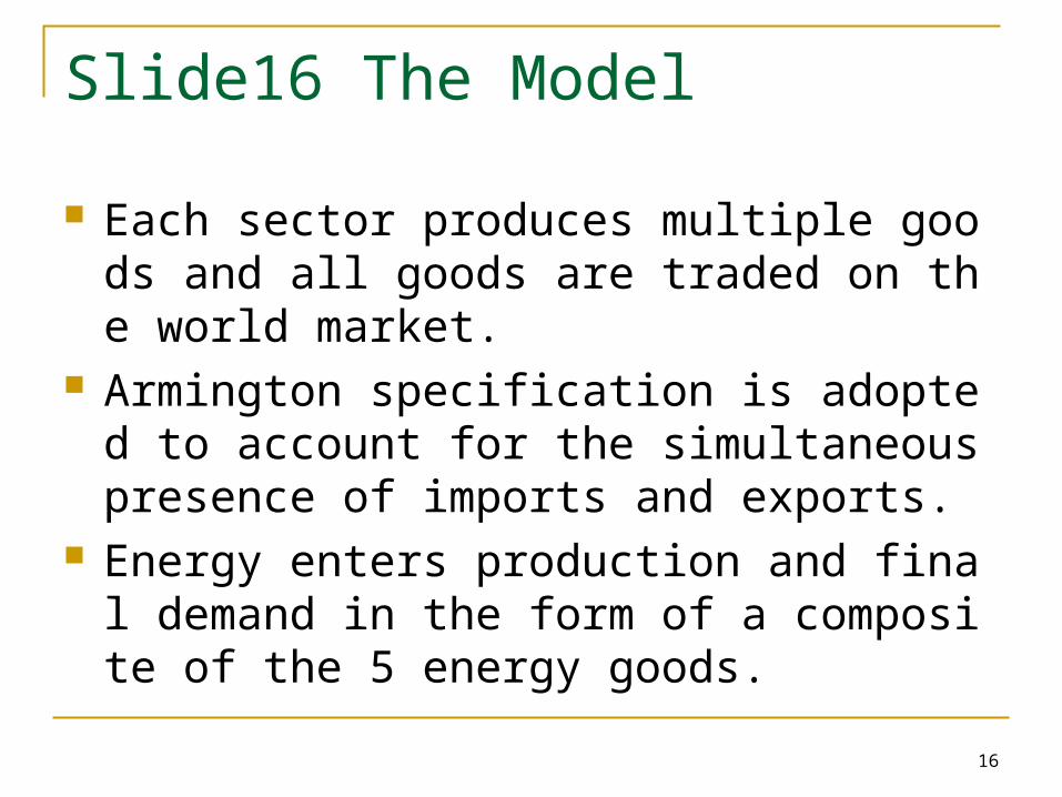
Slide16 The Model
Each sector produces multiple goods and all goods are traded on the world market.
Armington specification is adopted to account for the simultaneous presence of imports and exports.
Energy enters production and final demand in the form of a composite of the 5 energy goods.

17
Slide17 The Model
Output in non-fossil-fuel production sector
Tobias N. Rasmussen (2003) “Modeling the economics of greenhouse gas abatement: An overlapping generations perspective” Review of Economic Dynamics
18
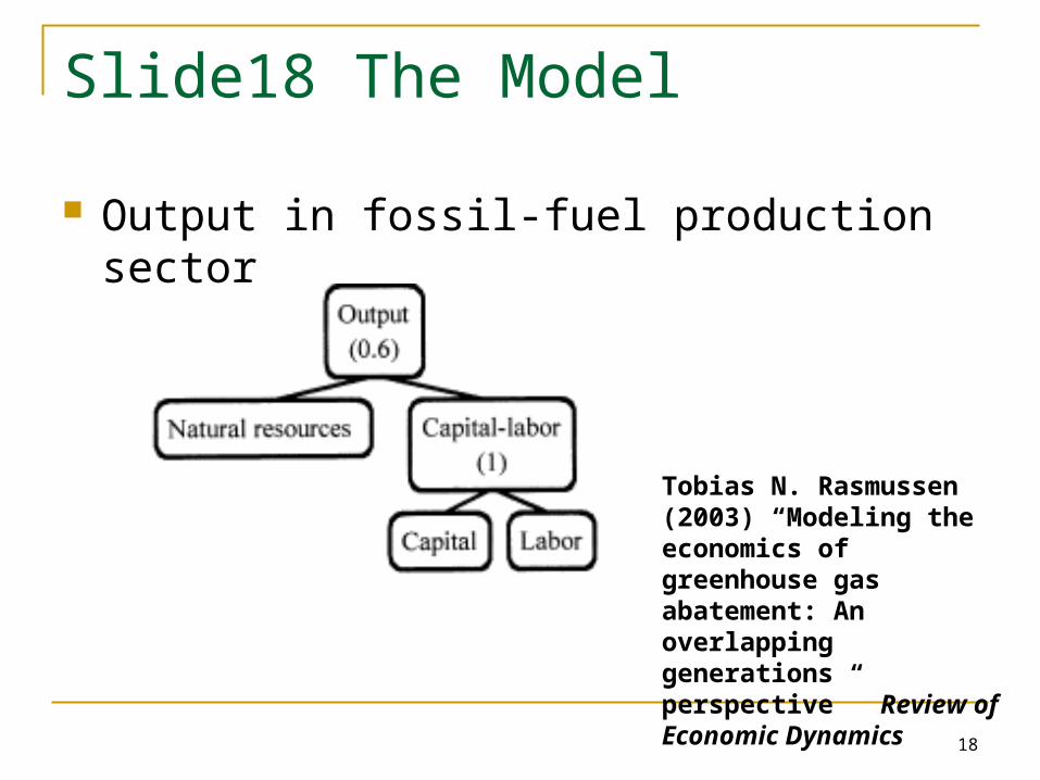
Slide18 The Model
Output in fossil-fuel production sector
Tobias N. Rasmussen (2003) “Modeling the economics of greenhouse gas abatement: An overlapping generations perspective” Review of Economic Dynamics
19
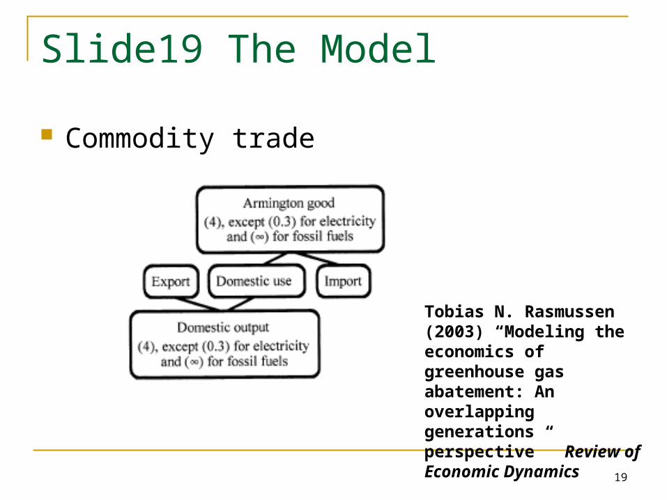
Slide19 The Model
Commodity trade
Tobias N. Rasmussen (2003) “Modeling the economics of greenhouse gas abatement: An overlapping generations perspective” Review of Economic Dynamics

20
Slide20 The Model
Energy for production and final demand
Tobias N. Rasmussen (2003) “Modeling the economics of greenhouse gas abatement: An overlapping generations perspective” Review of Economic Dynamics

21
Slide21 The Model
Household- each generation enters the model (at age 20) and die (at
age 80) at the end of year g + N (N=59).
- each generation chooses consumption and leisure to maximize his/her intertemporal utility.

22
Slide22 The Model
t , gt , gt , g
59g
gtt , g
Ftt , gt , gtt , g
59g
gt
Ct
σ-11
σ-1t , g
σ-1t , gt , g
ε-1t , g
g-t59g
gtt , gg
ωlwll
)transferplwe(wcp
)llφ-(1cφz to subject
ε-1
z
ρ11
t),(zu max
c: consumption, ll: leisure, ρ: discount rate, ε: the inverse of intertemporal elasticity of substitution, φ: weight on consumption, σ: the inverse of the elasticity of substitution between consumption and leisure, e: age-related productivity profile, ω: time endowment in efficiency units, pC: the price index for composite goods, transfer: a lump sum transfer.
c: consumption, ll: leisure, ρ: discount rate, ε: the inverse of intertemporal elasticity of substitution, φ: weight on consumption, σ: the inverse of the elasticity of substitution between consumption and leisure, e: age-related productivity profile, ω: time endowment in efficiency units, pC: the price index for composite goods, transfer: a lump sum transfer.

23
Slide23 The Model
Household demand structure
Tobias N. Rasmussen (2003) “Modeling the economics of greenhouse gas abatement: An overlapping generations perspective” Review of Economic Dynamics

24
Slide24 The Model
Model Closure
- (i) Trade balance
X: export, M: import, CAS: current account surplus at bench year, γ: effective growth rate
X: export, M: import, CAS: current account surplus at bench year, γ: effective growth rate
2000t
jt , j
jt , j CAS)γ(1M-X

25
Slide25 The Model
(ii) government budget balance
t20002000
t
jt , j
Ft , j
Mj
ht , h
Yh
Yhtt
Kttt
Lt
)γ(1GDEF-G)γ(1
MpτYpτKrτLwτ
τL: labor tax, L: aggregate labor, τK: interest rate tax, r: interest rate, K: aggregate capital stock, τh
K: commodity tax in sector h, phK: outp
ut prices in sector h, Yh: output in sector h, τjM : import tax of goods
j, pjF: import prices of goods j, G2000: government expenditure level a
t bench year, GDEF2000: government deficit level at bench year.

26
Slide26 The Model
Dynamic Equilibrium Condition
condition mequilibriu dynamic )δγYR()δ I(r
IYR
)Kδγ( I, )Kδ(rYR
YR: capital income at bench year, δ: depression rate, I: investment expenditure at bench year.
YR: capital income at bench year, δ: depression rate, I: investment expenditure at bench year.

27
Slide27 Simulation
CO2 emission
0
0.5
1
1.5
2
2.5
3
3.5
4
20
00
20
05
20
10
20
15
20
20
20
25
20
30
20
35
20
40
20
45
20
50
20
55
20
60
20
65
20
70
20
75
20
80
20
85
20
90
20
95
21
00
Benchmark Kyoto comittment

28
Slide28 Simulation
Tax on CO2 emission (thousand yen/metric ton of carbon)

29
Slide29 Simulation
Consumption level (% change from baseline)
-7
-6
-5
-4
-3
-2
-1
0
2000
2005
2010
2015
2020
2025
2030
2035
2040
2045
2050
2055
2060
2065
2070
2075
2080
2085
2090
2095
2100

30
Slide30 Simulation
Equivalent variation by generations (% change from baseline)
-3.5
-3
-2.5
-2
-1.5
-1
-0.5
0
20
00
20
05
20
10
20
15
20
20
20
25
20
30
20
35
20
40
20
45
20
50
20
55
20
60
20
65
20
70
20
75
20
80
20
85
20
90
20
95
21
00

31
Slide31 ILA model
1-γ1r1
ρ~
ε-1z
ρ~1
1)(zu max
ε
ε-1t
g-t
0ttg
)(

32
Slide32 Comparative Analysis Consumption level (% change from baseline)
-7
-6
-5
-4
-3
-2
-1
0
20
00
20
05
20
10
20
15
20
20
20
25
20
30
20
35
20
40
20
45
20
50
20
55
20
60
20
65
20
70
20
75
20
80
20
85
20
90
20
95
21
00

33
Slide33 Comparative Analysis Equivalent variation by generations (% change from baseline)
-3.5
-3
-2.5
-2
-1.5
-1
-0.5
0
20
00
20
05
20
10
20
15
20
20
20
25
20
30
20
35
20
40
20
45
20
50
20
55
20
60
20
65
20
70
20
75
20
80
20
85
20
90
20
95
21
00

34
Slide34 Main Conclusions
The cost of greenhouse gas emission abatement policy is distributed between generations unequally; small for current generations, large for future generations.
- in the OLG setup, each generation maximizes ONLY his/her own utility, NOT his/her descendants’.
- the reduction cost of CO2 abatement would rise rapidly, because we need to consume more fossil fuel in the process economy evolve under the constant technical level.