Embed Size (px)
Citation preview
On The Economic Order Quantity Model With Transportation Costs
S.I. Birbil, K. Bulbul, J.B.G. FrenkFaculty of Engineering and Natural Sciences,
Sabancı University, 34956 Istanbul, Turkey.
[email protected], [email protected], [email protected]
H.M. MulderErasmus University Rotterdam,
Postbus 1738, 3000 DR Rotterdam, The Netherlands.
Abstract: We consider an economic order quantity type model with unit out-of-pocket holding costs, unit
opportunity costs of holding, fixed ordering costs and general transportation costs. For these models, we analyze
the associated optimization problem and derive an easy procedure for determining a bounded interval containing
the optimal cycle length. Also for a special class of transportation functions, like the carload discount schedule, we
specialize these results and give fast and easy algorithms to calculate the optimal lot size and the corresponding
optimal order-up-to-level.
Keywords: EOQ-type model; transportation cost function; upper bounds; exact solution.
1. Introduction. In inventory control the economic order quantity model (EOQ) is the most funda-
mental model, which dates back to the pioneering work of Harris [8]. The environment of the model is
somewhat restricted. The demand is known and constant, shortages are not permitted, there is a fixed
setup cost and the unit purchasing and holding costs are independent of the size of the replenishment
order. In this simplest form, the model describes the trade-off between the fixed setup and the holding
costs. In the single item inventory control literature a lot of effort was put into weakening these assump-
tions [7, 14]. However, as noticed by Carter [5] most of these models did not take into consideration
the impact of the transportation costs as a separate cost component on the lot sizing decision. Carter
observes that typically in the lot sizing literature it is assumed that the transportation costs are managed
by the supplier (and hence part of the unit costs) or the transportation costs are fixed (and therefore
part of the setup costs). Carter presents some examples, in which it is clear that the transportation costs
should be taken into consideration differently. Actually, only one paper by Lee [11] is known to the
authors that incorporates a special transportation cost function (a freight discount rate charge) into the
classical EOQ model, where no shortages are allowed. The aim of the present paper is to include, in
a systematic way, the transportation costs as a separate cost component into an EOQ-type model and
investigate for which transportation cost functions it is still relatively simple to solve the corresponding
optimization problem. One of the most well-known transportation cost functions is the carload discount
schedule [12]. We present a detailed analysis for this particular schedule and related transportation
functions.
The problem setting is as follows: We consider an EOQ-type model with complete backordering,
where λ > 0 is the arrival rate and a > 0 is the fixed ordering cost. The inventory holding costs consist
of a unit out-of-pocket holding cost of h > 0 per item per unit of time and a unit opportunity cost of
holding with inventory carrying charge r ≥ 0. Moreover, the penalty cost of backlogging is b > 0 per
item per unit of time. To avoid pathological cases we assume that b > h. Clearly, when b = ∞ there
1
2 Birbil, Bulbul, Frenk, Mulder: EOQ with transportation costsTechnical Report, c©July 13, 2009
are no shortages in the problem. The function p : [0,∞) → R with p(0) = 0 represents the purchase
price function, and it is assumed that p(·) is left continuous on (0,∞). This means that the well-known
all-units-discount scheme [14] is also included in, especially the first part of, our analysis. At the same
time, the function t : [0,∞)→ Rwith t(0) = 0, denotes the transportation cost function and this function
is also assumed to be left continuous on (0,∞). The structure of the function t(·) allows us to model truck
costs. Consequently, the total transportation-purchase cost of an order of size Q is given by
c(Q) := t(Q) + p(Q), (1)
where c(·) denotes the transportation-purchase function. Since the addition of two left continuous
functions is again left continuous, the function c(·) is, in general, a left continuous function. This means
for every Q > 0 that
c(Q) = c(Q−) := limx↑Q c(x)
and
c(Q+) := limx↓Q c(x).
Using this left continuous transportation-purchase function c(·) implies that the cost rate function of an
EOQ-type model is given by
f (T, x) =
u(T)x, if x ≥ 0;
−bx, if x < 0,(2)
with
u(T) := h + r(λT)−1c(λT). (3)
For a detailed discussion of this cost rate function within a production environment, the reader is referred
to [2]. Since it is easy to see that for a given cycle length T > 0, any order-up-to-level S > λT is dominated
in cost by S = λT, we only derive the average cost expression for (S,T) control rules within the interval
0 ≤ S ≤ λT. For such control rules, the average cost g(S,T) has the form
g(S,T) =a + c(λT) +
∫ T
0f (T, S − λt)dt
T. (4)
Hence, to determine the optimal (S,T) rule, we need to solve the optimization problem
min{g(S,T) : T > 0, 0 ≤ S ≤ λT}.
By relation (4), this problem reduces to
min
{
a + c(λT) + ϕ(T)
T: T > 0
}
,
where ϕ : (0,∞)→ R is given by
ϕ(T) = min
{∫ T
0
f (T, S − λt)dt : 0 ≤ S ≤ λT
}
. (5)
Since by relation (2) it is easy to verify for 0 ≤ S ≤ λT that∫ T
0
f (T, S − λt)dt =λ−1u(T)S2
2+λ−1b(S − λT)2
2, (6)
and the derivative of this function for T fixed is equal to λ−1u(T)S+ λ−1b(S− λT), the optimal value S(T)
of the optimization problem listed in relation (5) is given by
S(T) =
bλTb+u(T) , for 0 < b < ∞;
λT, for b = ∞.
Birbil, Bulbul, Frenk, Mulder: EOQ with transportation costsTechnical Report, c©July 13, 2009
3
Hence, we obtain by relation (6) that
ϕ(T) =
λbu(T)T2
2(b+u(T)) , for 0 < b < ∞;λu(T)T2
2 , for b = ∞.
This shows by relation (3) for b < ∞ (shortages are allowed) that we need to solve the optimization
problem
min{Φb(T) : T > 0},
where
Φb(T) :=a + c(λT)
T+
bλT
2− (λbT)2
2λ(b + h)T + 2rc(λT). (7)
Similarly for b = ∞ (no shortages allowed), we obtain the optimization problem
min{Φ∞(T) : T > 0},
where
Φ∞(T) :=a + c(λT)
T+
hλT + rc(λT)
2. (8)
By the additivity of the costs, it is obvious that including the left continuous transportation-purchase
function c(·) as a separate cost component into the EOQ-type models does not change the structural
form of the objective function. However, since c(·) is left continuous, we can only conclude that the
objective functions in relations (7) and (8) are also left continuous, and hence, they may contain points
of discontinuity. In general, these functions (as a function of the length of the replenishment cycle T) are
not unimodal anymore as in the classical EOQ models. Hence, they may contain several local minima
and so, it might be difficult to guarantee that a given solution is indeed optimal.
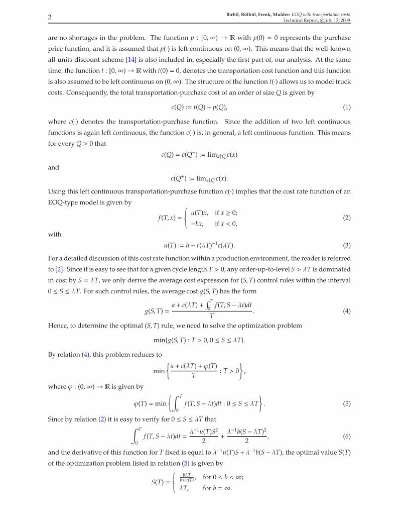
Our approach to these general models is to derive, in Section 2, a bounded interval containing the
optimal cycle length T. We will first construct an upper bound on the optimal solution for a left
continuous and increasing transportation-purchase function as shown in Figure 1(a). This upper bound
is represented by an easy analytical formula for the special case of an increasing polyhedral concave
transportation-purchase function. Such a function is shown in Figure 1(c) and represents a typical
economies of scale situation. For the other more general transportation-purchase functions, it is possible
to evaluate this upper bound by an algorithm. However, since this might take some computational
time, we also derive under some reasonable bounding condition on a transportation-purchase function,
a weaker analytical upper bound. To improve the trivial zero bound on an optimal solution, we
only derive for an increasing concave transportation-purchase function as illustrated in Figure 1(b), an
analytical positive lower bound.
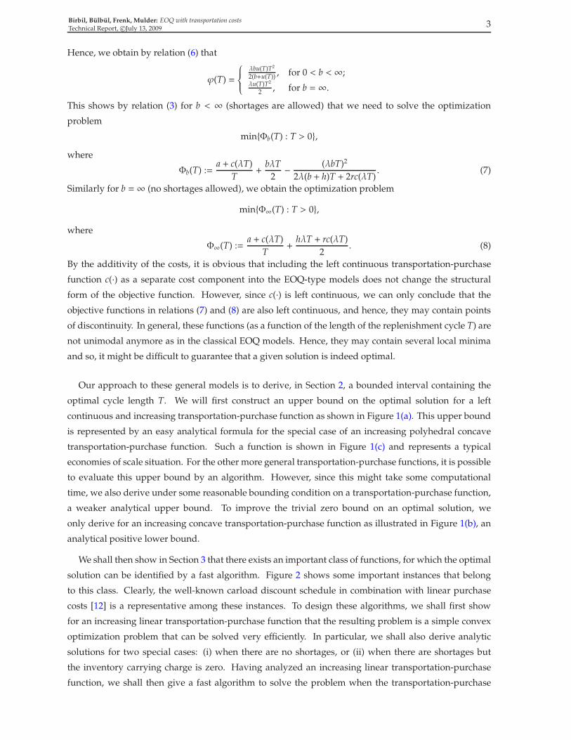
We shall then show in Section 3 that there exists an important class of functions, for which the optimal
solution can be identified by a fast algorithm. Figure 2 shows some important instances that belong
to this class. Clearly, the well-known carload discount schedule in combination with linear purchase
costs [12] is a representative among these instances. To design these algorithms, we shall first show
for an increasing linear transportation-purchase function that the resulting problem is a simple convex
optimization problem that can be solved very efficiently. In particular, we shall also derive analytic
solutions for two special cases: (i) when there are no shortages, or (ii) when there are shortages but
the inventory carrying charge is zero. Having analyzed an increasing linear transportation-purchase
function, we shall then give a fast algorithm to solve the problem when the transportation-purchase

4 Birbil, Bulbul, Frenk, Mulder: EOQ with transportation costsTechnical Report, c©July 13, 2009
c(Q)
Q
(a) General
c(Q)
Q
(b) Concave
c(Q)
Q
(c) Polyhedral concave
Figure 1: Some transportation-purchase functions for which the bounds on optimal T are studied.
function is increasing piecewise polyhedral concave as shown in Figure 2(a). This algorithm is based
on solving a series of simple problems that correspond to the increasing linear pieces on the piecewise
polyhedral concave function. To further improve the performance of the proposed algorithm, we
shall then concentrate on two particular instances as shown in figures 2(b) and 2(c). The former is a
typical carload schedule with identical setups, and the latter represents a general carload schedule with
nonincreasing truck setup costs. Both cases admit a lower bounding function, which is linear in the
former case and polyhedral concave in the latter case. These lower bounding functions, shown with
dashed lines in Figure 2, allow us to concentrate on solving only a very few simple problems. Finally, in
Section 4 we will give some numerical examples to illustrate our results.
c(Q)
Q
(a) Piecewise polyhedral concave
Q
c(Q)
(b) Typical carload schedule
c(Q)
Q
(c) General carload schedule
Figure 2: Some transportation-purchase functions for which fast algorithms are developed.
2. Bounding The Optimal Cycle Length. In this section we show that one can identify an upper
bound on the optimal cycle length of the previous EOQ-type models for left continuous increasing
transportation-purchase functions c(·) as shown in Figure 1(a). For very general functions c(·), it might
be difficult to compute this upper bound by means of an easy algorithm. Therefore, we show that under
an affine bounding condition on the function c(·), this upper bound can be replaced by a weaker upper
bound having an elementary formula. To derive these results, we first identify the general structure of
the considered EOQ-type models.
Birbil, Bulbul, Frenk, Mulder: EOQ with transportation costsTechnical Report, c©July 13, 2009
5
Let F : [0,∞)× (0,∞)→ R be given by
F(x,T) :=a + x
T+
bλT
2− (λbT)2
2λ(h + b)T + 2rx, (9)
then it follows from relation (7) that the EOQ-type optimization problem with shortages is given by
min{F(c(λT),T) : T > 0}. (Pb)
Similarly, we also introduce the function G : [0,∞)× (0,∞)→ R given by
G(x,T) :=a + x
T+
hλT + rx
2. (10)
Then, it is clear from relation (8) that the EOQ-type model with no shortages allowed (b = ∞) transforms
to
min{G(c(λT),T) : T > 0}. (P∞)
By relations (9) and (10), it is obvious that the functions F(·, ·) and G(·, ·) belong to the following class of
functions.
Definition 2.1 A function H : [0,∞) × (0,∞) → R belongs to the set H if the function H(·, ·) is continuous,
x 7→ H(x,T) is increasing on [0,∞) for every T > 0, and limT↓0 H(x,T) = limT↑∞H(x,T) = ∞ for every x ≥ 0.
Hence, both EOQ-type optimization models are particular instances of the optimization problem
min{H(c(λT),T) : T > 0}, (P)
where H(·, ·) belongs to the set H and c(·) is an increasing left continuous function on [0,∞). We show
in Lemma A.1 of Appendix A that the function T 7→ H(c(λT),T) is lower semi-continuous for any H(·, ·)belonging toH . Consequently, an optimal solution for problem (P) indeed exists, and hence, our search
for a bounded interval containing an optimal solution is justified.
2.1 Dominance Results. In this section, we shall give two simple dominance results that will be
instrumental for finding a bounded interval for different EOQ-type models. We start with the following
lemma, which has a straightforward proof. The functions c(·) and c1(·) satisfying the conditions of the
lemma are exemplified in Figure 3.
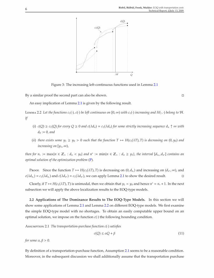
Lemma 2.1 Let the functions c1(·), c(·) be left continuous on [0,∞) with c1(·) increasing and H(·, ·) belong toH .
(i) If c(Q) ≥ c1(Q) for every Q > λd and c(λd) = c1(λd) and T 7→ H(c1(λT),T) is increasing on (d,∞), then
H(c(λT),T) ≥ H(c(λd), d) for every T > d.
(ii) If c(Q) ≥ c1(Q) for every Q ≤ λd and c(λd) = c1(λd) and T 7→ H(c1(λT),T) is decreasing on (0, d), then
H(c(λT),T) ≥ H(c(λd), d) for every T < d.
Proof. Since the function H(·, ·) belongs toH and the function c1(·) is left continuous and increasing,
it follows that
limT↓d H(c1(λT),T) = H(c1((λd)+), d) ≥ H(c1(λd), d) = H(c(λd), d).
Using again H(·, ·) ∈ H , c(λT) ≥ c1(λT) for every T > d, and T 7→ H(c1(λT),T) is increasing on (d,∞), we
have for every T > d that
H(c(λT),T) ≥ H(c1(λT),T) ≥ limT↓d H(c1(λT),T) ≥ H(c(λd), d).
6 Birbil, Bulbul, Frenk, Mulder: EOQ with transportation costsTechnical Report, c©July 13, 2009
Q
c(Q)
λd
c1(Q)
Figure 3: The increasing left-continuous functions used in Lemma 2.1
By a similar proof the second part can also be shown. �
An easy implication of Lemma 2.1 is given by the following result.
Lemma 2.2 Let the functions c1(·), c(·) be left continuous on [0,∞) with c1(·) increasing and H(·, ·) belong toH .
If
(i) c(Q) ≥ c1(Q) for every Q ≥ 0 and c(λdn) = c1(λdn) for some strictly increasing sequence dn ↑ ∞ with
d0 := 0, and
(ii) there exists some y1 ≥ y0 > 0 such that the function T 7→ H(c1(λT),T) is decreasing on (0, y0) and
increasing on [y1,∞),
then for n∗ := max{n ∈ Z+ : dn < y0} and n∗ := min{n ∈ Z+ : dn ≥ y1}, the interval [dn∗ , dn∗] contains an
optimal solution of the optimization problem (P).
Proof. Since the function T 7→ H(c1(λT),T) is decreasing on (0, dn∗) and increasing on (dn∗ ,∞), and
c(λdn∗) = c1(λdn∗ ) and c(λdn∗ ) = c1(λdn∗), we can apply Lemma 2.1 to show the desired result. �
Clearly, if T 7→ H(c1(λT),T) is unimodal, then we obtain that y1 = y0 and hence n∗ = n∗ + 1. In the next
subsection we will apply the above localization results to the EOQ-type models.
2.2 Applications of The Dominance Results to The EOQ-Type Models. In this section we will
show some applications of Lemma 2.1 and Lemma 2.2 on different EOQ-type models. We first examine
the simple EOQ-type model with no shortages. To obtain an easily computable upper bound on an
optimal solution, we impose on the function c(·) the following bounding condition.
Assumption 2.1 The transportation-purchase function c(·) satisfies
c(Q) ≤ αQ + β (11)
for some α, β > 0.
By definition of a transportation-purchase function, Assumption 2.1 seems to be a reasonable condition.
Moreover, in the subsequent discussion we shall additionally assume that the transportation purchase
Birbil, Bulbul, Frenk, Mulder: EOQ with transportation costsTechnical Report, c©July 13, 2009
7
function c(·) is increasing. Notice that the analysis up to this point applies to any type of EOQ-type
model, but with this monotonicity assumption on c(·) we exclude the all-units discount model.
c(λT)
−a
D
d
c1(λT)
c(λd) = c1(λd)
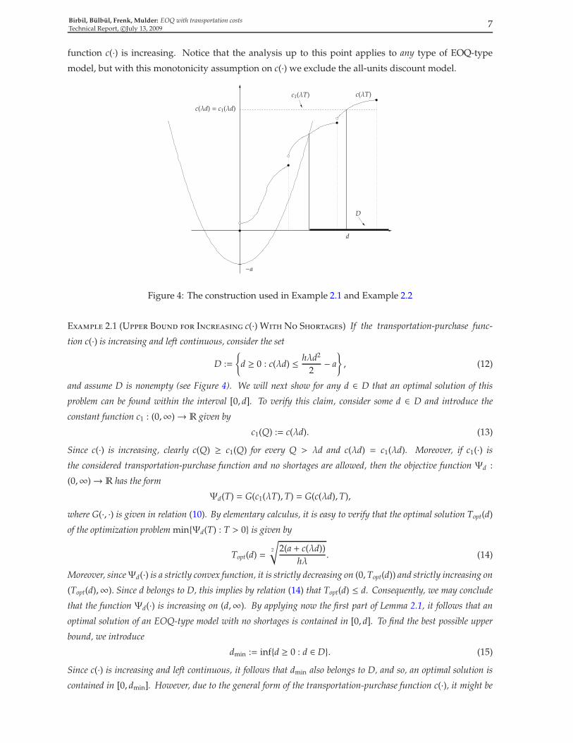
Figure 4: The construction used in Example 2.1 and Example 2.2
Example 2.1 (Upper Bound for Increasing c(·) WithNo Shortages) If the transportation-purchase func-
tion c(·) is increasing and left continuous, consider the set
D :=
{
d ≥ 0 : c(λd) ≤ hλd2
2− a
}
, (12)
and assume D is nonempty (see Figure 4). We will next show for any d ∈ D that an optimal solution of this
problem can be found within the interval [0, d]. To verify this claim, consider some d ∈ D and introduce the
constant function c1 : (0,∞)→ R given by
c1(Q) := c(λd). (13)
Since c(·) is increasing, clearly c(Q) ≥ c1(Q) for every Q > λd and c(λd) = c1(λd). Moreover, if c1(·) is
the considered transportation-purchase function and no shortages are allowed, then the objective function Ψd :
(0,∞)→ R has the form
Ψd(T) = G(c1(λT),T) = G(c(λd),T),
where G(·, ·) is given in relation (10). By elementary calculus, it is easy to verify that the optimal solution Topt(d)
of the optimization problem min{Ψd(T) : T > 0} is given by
Topt(d) =2
√
2(a + c(λd))
hλ. (14)
Moreover, sinceΨd(·) is a strictly convex function, it is strictly decreasing on (0,Topt(d)) and strictly increasing on
(Topt(d),∞). Since d belongs to D, this implies by relation (14) that Topt(d) ≤ d. Consequently, we may conclude
that the function Ψd(·) is increasing on (d,∞). By applying now the first part of Lemma 2.1, it follows that an
optimal solution of an EOQ-type model with no shortages is contained in [0, d]. To find the best possible upper
bound, we introduce
dmin := inf{d ≥ 0 : d ∈ D}. (15)
Since c(·) is increasing and left continuous, it follows that dmin also belongs to D, and so, an optimal solution is
contained in [0, dmin]. However, due to the general form of the transportation-purchase function c(·), it might be

8 Birbil, Bulbul, Frenk, Mulder: EOQ with transportation costsTechnical Report, c©July 13, 2009
difficult to give a fast procedure to compute the value of dmin. To replace dmin by an easy computable bound, we now
use Assumption 2.1 as c(λd) ≤ αλd + β. Observe this bounding condition guarantees that the set D is nonempty
and{
d ≥ 0 : αλd + β ≤ hλd2
2− a
}
⊆ D. (16)
Since it is easy to see that {d ≥ 0 : αλd + β ≤ hλd2
2 − a} = [vα,β,∞) with
vα,β := αh−1 +2
√
α2h−2 + 2h−1λ−1(a + β), (17)
we obtain by relation (16) that
vα,β ≥ dmin. (18)
Therefore, an optimal solution is contained in (0, vα,β].
Due to the specific form of the function c1(·), it follows by relation (10) that for the EOQ-type model with
no shortages and transportation-purchase function c1(·), the inventory carrying charge is a fixed cost
independent of the decision variable T. Hence, the optimal Topt(d) given by relation (14) does not contain
the value of r. This means for our procedure discussed in Example 2.1 that the constructed upper bound
on an optimal solution does not contain this parameter r and holds uniformly for every r ≥ 0. Hence, it
seems likely that this upper bound might be far away from an optimal solution of an EOQ-type model
with function c(·) and a given inventory carrying charge. We explore this issue by our computational
study in Section 4. In case we do not have any structure on c(·) –the structured case will be considered
in the next section– we might now use some discretization method over (0,wα,β] to approximate the
optimal solution for the no shortages case.
We shall consider next the general EOQ-type model with shortages. Before discussing the construction
of an upper bound for this model, we first need the following result.
Lemma 2.3 If T(r)opt(d) denotes the optimal solution of the EOQ model with shortages allowed, inventory carrying
charge r ≥ 0 and the constant transportation-purchase function c1(·) listed in relation (13), then for all r ≥ 0, we
have
T(r)opt(d) ≤ T(0)
opt(d) =
√
2(a + c(λd))
hλ
h + b
b.
Proof. The objective function of the considered EOQ-model with inventory carrying charge r > 0 is
given by T 7→ F(c1(λT),T) with F(·, ·) listed in relation (9). Since it is easy to check for every x ≥ 0 that
(λbT)2
2λ(h + b)T + 2rx=λb2
2(h + b)
(
T − rxT
λ(h + b)T + rx
)
,
we have
F(c1(λT),T) =a + c(λd)
T+
b
h + b
λhT
2+λb2r
2(h + b)
(
c(λd)T
λ(h + b)T + rc(λd)
)
. (19)
Introducing now the convex function T 7→ F0(c1(λT),T) with
F0(x,T) :=a + x
T+
b
h + b
λhT
2
and the increasing function K : (0,∞)→ R given by
K(T) :=λb2r
2(h + b)
(
c(λd)T
λ(h + b)T + rc(λd)
)
,
Birbil, Bulbul, Frenk, Mulder: EOQ with transportation costsTechnical Report, c©July 13, 2009
9
we obtain by relation (19) that
F(c1(λT),T) = F0(c1(λT),T) + K(T). (20)
By looking at relation (20), we observe that the function
T 7→ F0(c1(λT),T)
is the objective function of an EOQ-model with shortages allowed, r = 0, and the transportation-purchase
function c1(·). Also, it is easy to check in relation (20) that the remainder function K is increasing with a
positive derivative. This shows that the derivative of the function
T 7→ F(c1(λT),T)
evaluated at the optimal solution T(0)opt(d) of an EOQ-type model with shortages allowed and r = 0 is
positive. Using now relation (9) with r = 0, it is easy to check that
T(0)opt(d) =
√
2(a + c(λd))
hλ
h + b
b.
Since by the definition of T(r)opt(d) the derivative of the function T → F(c1(λT),T) evaluated at this point
equals 0, the inequality
T(r)opt(d) ≤ T(0)
opt(d)
holds once we have verified that the function T 7→ F(c1(λT),T) is unimodal. To show this property, we
first observe that the function K1 : (0,∞)→ R given by
K1(T) := TK(T)
being the ratio of a squared convex function and an affine function is convex [4]. This implies that
the function T 7→ TK1(T−1) = K(T−1) is convex [9]. Moreover, it is easy to verify by its definition
that the function T 7→ F0(c1(λT−1),T−1) is convex, and this shows by relation (20) that the function
T 7→ F(c1(λT−1),T−1) is convex implying T 7→ F(c1(λT),T) is unimodal. �
Lemma 2.3 shows that the optimal solution of an EOQ-type model with the constant transportation-
purchase function c1(·) and nonzero inventory carrying charge is bounded from above by the optimal
solution of an EOQ-type model with the transportation-purchase function c1(·) and zero inventory
carrying charge. Using this result we will construct in the next example an upper bound on the
optimal solution of an EOQ-type model with shortages allowed, inventory carrying charge r ≥ 0 and
left-continuous increasing transportation-purchase function c(·).
Example 2.2 (Upper Bound for Increasing c(·) With Shortages) If the transportation-purchase function c(·)is increasing and left continuous, consider the set
D :=
{
d ≥ 0 : c(λd) ≤ hλd2
2
b
h + b− a
}
, (21)
and assume that D is nonempty (see also Figure 4). Let d ∈ D and consider the constant function c1 : (0,∞)→ Rgiven by
c1(Q) := c(λd).
Since c is increasing clearly c(Q) ≥ c1(Q) for every Q > λd and c(λd) = c1(λd). Moreover, if shortages are
allowed, then the objective functionΨd : (0,∞)→ R has the form
Ψd(T) = F(c1(λT),T) = F(c(λd),T),

10 Birbil, Bulbul, Frenk, Mulder: EOQ with transportation costsTechnical Report, c©July 13, 2009
where F(·, ·) is given in relation (9). In the proof of Lemma 2.3, it is shown that the objective function Ψd is
unimodal, and for any r ≥ 0 we have
T(r)opt(d) ≤ T
(0)opt(d) =
2
√
2(a + c(λd))
λh
h + b
b. (22)
Applying now the unimodality of the functionΨd(·) this yields thatΨd(·) is increasing on the interval (T(r)opt(d),∞),
and since d belongs to D, we also obtain by relation (22) that
T(r)opt(d) ≤ T
(0)opt(d) ≤ d.
This shows that the functionΨd(·) is increasing on (d,∞), and by applying part (i) of Lemma 2.1, we conclude that
an optimal solution of the EOQ-type model with the general transportation-purchase function c(·) is contained in
the interval [0, d]. As in Example 2.1 the best possible upper bound is now given by
dmin := inf{d ≥ 0 : d ∈ D}. (23)
Again due to the particular instance of c(·) it might be difficult to compute dmin. To replace dmin by an easily
computable upper bound, we again use the bounding condition given in Assumption 2.1 and obtain c(λd) ≤ αλd+β.
This implies that D is nonempty and it follows as in Example 2.1 that dmin ≤ wα,β with
wα,β := αh−1(h + b)b−1 +2
√
α2h−2((h + b)b−1)2 + 2h−1λ−1(a + β)(h + b)b−1. (24)
Therefore, under the bounding condition, wα,β serves as an upper bound on an optimal solution of the original
problem.
Remark 2.1 By relations (12) and (21), it is easy to see that an upper bound on an optimal solution for an
EOQ-type model with no shortages (Example 2.1) is always smaller than an upper bound on an optimal solution
of an EOQ-type model with shortages (Example 2.2). Similarly, we obtain by relations (17) and (24) that this also
holds for the easily computable upper bounds under the bounding condition.
In case we additionally know that the function c(·) is concave, which corresponds to some incremental
discount scheme [14] for either the purchase function or the transportation cost function, it is also possible
to compute a (nontrivial) lower bound on the optimal solutions of the EOQ-type models considered in
the previous two examples. The next example discusses this lower bound explicitly for the no shortages
case.
Example 2.3 (Lower Bound for Increasing Concave c(·) WithNo Shortages) If we know additionally
that the transportation-purchase function c(·) is concave, and hence continuous, it is also possible to give a
lower bound on the optimal solution. Observe in this case that Assumption 2.1 is trivially satisfied (see Figure 5).
Take for simplicity, Q 7→ c(λd)λd Q + c(λd), which clearly satisfies Assumption 2.1 with α =
c(λd)λd and β = c(λd).
Consider now for d > 0, the function c1 : (0,∞)→ R given by
c1(Q) =c(λd)
λdQ.
By the concavity of c(·) and c(0) = 0, we obtain for every Q < λd that
c(Q) = c(Qλ−1d−1λd) ≥ Qλ−1d−1c(λd)

Birbil, Bulbul, Frenk, Mulder: EOQ with transportation costsTechnical Report, c©July 13, 2009
11
Q
c(Q)
λd
c1(Q)
c(λd) = c1(λd)
Figure 5: The construction used in Example 2.3
and this shows c(Q) ≥ c1(Q) for every Q < λd and c(λd) = c1(λd). As in Example 2.1 the objective function has
the form
Ψd(T) = G(c1(λT),T)
where G(·, ·) is given in relation (10). By elementary calculus, it is easy to verify that the optimal solution Topt(d)
of the optimization problem min{Ψd(T) : T > 0} is given by
Topt(d) = 2
√
2a
hλ + rc(λd)d−1. (25)
Since the function x 7→ c(λx)x−1 is decreasing and continuous with limx↓0 c(λx)x−1 ≤ ∞, it follows by relation
(25) that the function Topt : (0,∞)→ R is increasing and continuous. Also, by the strict convexity of the function
Ψd this function is strictly decreasing on (0,Topt(d)) and strictly increasing on (Topt(d),∞). This implies
Ψd decreasing on (0, d)⇔ Topt(d) ≥ d.
Since the set {d ≥ 0 : Topt(d) ≥ d} contains 0 it follows by the second part of Lemma 2.1 that an optimal solution of
the EOQ-type model with no shortages allowed and a concave transportation-purchase function c(·) is contained
in [dmax,∞), where
dmax := sup{d ≥ 0 : Topt(d) ≥ d} = sup{d ≥ 0 : hλd2 + rdc(λd) ≤ 2a}. (26)
Since the function d 7→ hλd2 + rdc(λd) is strictly increasing and continuous on [0,∞), we obtain that dmax is the
unique solution of the system
hλx2 + rxc(λx) = 2a.
Also, by the nonnegativity of c we obtain that
dmax ∈ [0,2√
2aλ−1h−1].
Thus, one can apply a computationally fast derivative free one-dimensional search algorithm [3] over the interval
of uncertainty [0,2√
2aλ−1h−1] to compute the lower bound dmax.
Since the derivation is very similar, we omit the lower bound for the shortages case.
12 Birbil, Bulbul, Frenk, Mulder: EOQ with transportation costsTechnical Report, c©July 13, 2009
As shown in the above examples, under the affine bounding condition stated in Assumption 2.1, it
is possible to identify by means of an elementary formula a bounded interval I containing an optimal
solution of the EOQ-type model with increasing transportation-purchase function c(·). Hence, we obtain
for the two different cases represented by the optimization problems (Pb) and (P∞) that
minT>0 H(c(λT),T) = minT∈I H(c(λT),T). (27)
However, for the general increasing left continuous transportation-purchase functions, the function
T 7→ H(c(λT),T) does not have the desirable unimodal structure. Since we are interested in finding an
optimal solution, the only thing we could do is to discretize the interval I and select among the evaluated
function values on this grid the one with a minimal value. In case the objective function has a finite
number of discontinuities and it is Lipschitz continuous between any two consecutive discontinuities
with known (maybe different) Lipschitz constants, it is possible by using an appropriate chosen grid to
give an error on the deviation of the objective value of this chosen solution from the optimal objective
value. We leave the details of this construction to the reader and refer to the literature on one-dimensional
Lipschitz optimization algorithms [10].
However, for some left continuous increasing transportation-purchase functions c(·), it is possible
to compute explicitly the value of dmin listed in relations (15) and (23) by means of an easy algorithm.
This means that for these functions we do not need the easily computable upper bound and so in
this case the upper bound on an optimal solution can be improved. An example of such a class of
transportation-purchase functions is given in the next definition.
Definition 2.2 ([13]) A function c : (0,∞)→ R is called a polyhedral concave function on (0,∞), if c(·) can be
represented as the minimum of a finite number of affine functions on (0,∞). It is called polyhedral concave on an
interval I, if c(·) is the minimum of a finite number of affine functions on I.
We will now give an easy algorithm to identify the value dmin in case c(·) is an increasing polyhedral
concave function. Observe it is easy to verify that polyhedral concave functions defined on the same
interval are closed under addition. Within the inventory theory, polyhedral concavity on [0,∞) of
the transportation-purchase function c(·) describes incremental discounting either with respect to the
purchase costs or the transportation costs or both.
Clearly, a polyhedral concave function on (0,∞) can be represented for every Q > 0 as
c(Q) = min1≤n≤N{αnQ + βn}, (28)
where N denotes the total number of affine functions, α1 > .... > αN ≥ 0, and 0 ≤ β1 < β2 < ... < βN. An
example of a polyhedral concave function c(·) is given in Figure 6. Between kn−1 and kn the minimum in
relation (28) is attained by the affine function Q 7→ αnQ + βn. To compute the values αn and βn in terms
of our original data given by the finite set of breaking points 0 = k0 < k1 < ... < kN−1 < kN = ∞, and
function values c(kn), n = 1, ...N − 1 we observe that
αn =c(kn) − c(kn−1)
kn − kn−1(29)
for n = 1, ...,N − 1 and
αN = c(kN−1 + 1) − c(kN−1). (30)

Birbil, Bulbul, Frenk, Mulder: EOQ with transportation costsTechnical Report, c©July 13, 2009
13
λdmin
α1
−a
c(Q)
Qk0 = 0 k1 k2 k3
β2
β3
β4
β1
α4
α3
α2
Figure 6: A polyhedral concave transportation-purchase function.
Also, by the same figure we obtain for kn−1 < Q ≤ kn, n = 1, ..,N that
c(Q) = c(kn−1) + αn(Q − kn−1) = αnQ + βn
and this implies
βn = c(kn−1) − αnkn−1 (31)
for n = 1, ..,N.
We will now give an easy algorithm to identify the value dmin, if c(·) is a polyhedral concave function
with the representation given in relation (28). Using now relations (15) and (23), we have
dmin = min{d > 0 : c(λd) ≤ hλd2ζ
2− a}, (32)
where ζ = 1 for the no shortages case and ζ = bh+b for the shortages case. Since c(·) is concave and
increasing, and the function d 7→ hλd2ζ2 − a is strictly convex and increasing on [0,∞) (see Figure 6), each
region D, given by relation (12) or relation (21), is an interval [dmin,∞). The next algorithm clearly yields
dmin as an output .
Algorithm 1: Finding dmin for polyhedral c(·)
n∗ := max{0 ≤ n ≤ N − 1 : c(kn) >hk2
nζ
2λ − a}1:
Determine in [kn∗ , kn∗+1] or in [kn∗ ,∞) the unique analytical solution d∗ of the equation2:
αn∗+1λd + βn∗+1 =hλd2ζ
2− a
given by
d∗ =αn∗+1λ +
√
(αn∗+1λ)2 + 2hλζ(a + βn∗+1)
hλζ
dmin ← d∗3:
In the next section we shall identify a subclass of the increasing left continuous transportation-
purchase functions, for which it is easy to identify an optimal solution instead of only a bounded
14 Birbil, Bulbul, Frenk, Mulder: EOQ with transportation costsTechnical Report, c©July 13, 2009
interval containing an optimal solution.
3. Fast Algorithms for Solving Some Important Cases. Unless we impose some additional structure
on c(·), it could be difficult to find a fast algorithm to solve optimization problem (P) due to the existence
of many local minima. Clearly, if c(·) is an affine function given by
c(Q) = αQ + β
with α > 0, β ≥ 0, it is already shown in [2] that the objective functions of both EOQ-type models given
by (Pb) and (P∞) are unimodal functions. Also for the no shortages model (P∞), it is easy to check by
relation (10) that the optimal solution Topt is given by
Topt =2
√
2(a + β)
λ(h + rα), (33)
while for the shortages model (Pb) with zero inventory carrying charge (r = 0), it follows by relation (9)
that the optimal solution Topt has the form
Topt =2
√
2(a + β)
λh
h + b
b. (34)
Finally, for the most general model with shortages allowed and nonzero inventory carrying charge, it
follows that the function
T 7→ F(c(λT−1,T−1)
is a convex function on [0,∞) (see [2, Lemma 3.2]). Hence, solving problem (Pb) using the decision
variable T−1 is an easy one-dimensional convex optimization problem, and so, we can find Topt rather
quickly. Consequently, this observation helps us to come up with fast algorithms when c(·) consists of
linear pieces. Among such functions, the most frequently used ones are the polyhedral concave functions
given in (28). Using this representation and H(·, ·) ∈ H , the overall objective function for both EOQ-type
models becomes
H(c(λT),T) = min1≤n≤N H(αnλT + βn,T). (35)
This shows by our previous observations that the function T 7→ H(c(λT−1),T−1) is simply the minimum
of N different convex functions. In general this function is not convex anymore and even not unimodal.
However, due to relation (35) it follows that
minT>0
H(c(λT−1),T−1) = min1≤n≤N
minT>0
H(αnλT−1 + βn,T−1), (36)
and by relation (36), we need to solve N one-dimensional unconstrained convex optimization problems
to determine an optimal solution. Notice by relation (35) that each of these N problems involve an affine
function. This implies that if we consider the no shortages model (Pb) or the shortages model (P∞) with
r = 0, then we have the analytic solutions (33) and (34), respectively. Therefore, solving (36) boils down
to selecting the minimum among N different values in these cases.
We next introduce a more general class containing as a subclass the polyhedral concave functions on
[0,∞). An illustration of a function in this class is given in Figure 7.
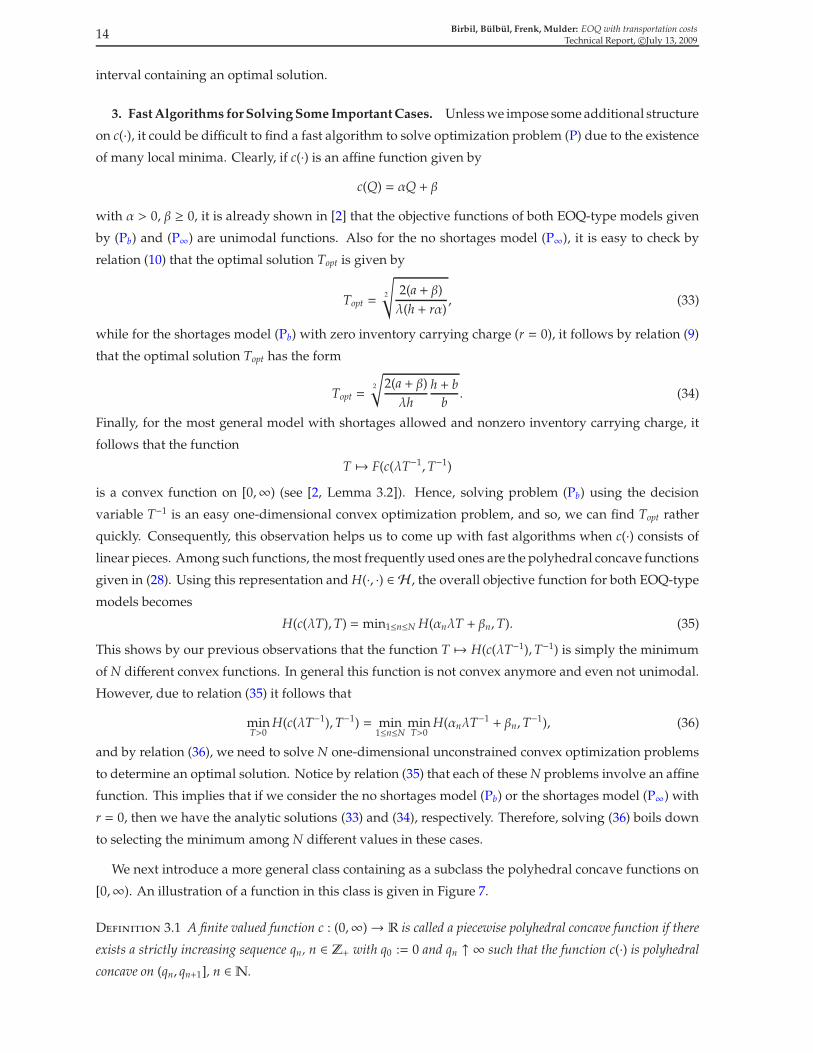
Definition 3.1 A finite valued function c : (0,∞)→ R is called a piecewise polyhedral concave function if there
exists a strictly increasing sequence qn, n ∈ Z+ with q0 := 0 and qn ↑ ∞ such that the function c(·) is polyhedral
concave on (qn, qn+1], n ∈N.
Birbil, Bulbul, Frenk, Mulder: EOQ with transportation costsTechnical Report, c©July 13, 2009
15
q0 q1 q2 q3
c(Q)
Q
Figure 7: A piecewise polyhedral concave transportation-purchase function.
A piecewise concave polyhedral function might be discontinuous at the points qn, n ∈ Z+. If the function
c(·) is a piecewise polyhedral concave function, then it follows by relation (28) that
c(Q) = min1≤n≤Nk
{αnkQ + βnk} (37)
for qk−1 < Q ≤ qk and finite Nk. If, additionally, the function c(·) satisfies Assumption 2.1, then we have
shown in Subsection 2.2 that an easily computable upper bound exists on the optimal solution. We
denote this upper bound by U. For problem (P∞), U is given by relation (17), while for problem (Pb) it is
given by relation (24). Since qn ↑ ∞ and U is a finite upper bound on an optimal solution it follows that
m∗ := min{n ∈N : qn > λU} < ∞ (38)
and an optimal solution is contained in the bounded interval [0, λ−1qm∗ ). Since c(·) is increasing this
implies that
minT>0 H(c(λT),T) = min0<T≤λ−1qm∗ H(c(λT),T)
= min1≤k≤m∗ minλ−1qk−1≤T≤λ−1qkH(c(λT),T).
By relation (37), it follows now that
minλ−1qk−1≤T≤λ−1qk
H(c(λT),T) = min1≤n≤Nk
minλ−1qk−1≤T≤λ−1qk
H(αnkλT + βnk,T),
and so, we have to solve for 1 ≤ k ≤ m∗ and n ≤ Nk, the constrained convex one-dimensional optimization
problems
minλ−1qk−1≤T≤λ−1qk
H(αnkλT−1 + βnk,T−1).
Solving these subproblems can be done relatively fast, but since we have to solve∑m∗
k=1 Nk of those
subproblems this might take a long computation time for the most general case. Observe once again, if
we only consider the no shortages model or the shortages model with zero inventory carrying charge,
the subproblems minT>0 H(αnkλT + βnk,T) have analytical solutions given by relations (33) and (34),
respectively. Hence, using the unimodality of the considered objective functions, the optimal solution
can be determined simply by checking whether the optimal solution of the unconstrained problem lies
within [λ−1qk−1, λ−1qk]. Hence, for the piecewise polyhedral transportation-purchase function, we have
the steps outlined in Algorithm 2.
16 Birbil, Bulbul, Frenk, Mulder: EOQ with transportation costsTechnical Report, c©July 13, 2009
Algorithm 2: Finding Topt for piecewise polyhedral c(·)
Determine U and determine m∗ by relation (38)1:
Solve for k = 1, ...,m∗ the optimization problems2:
ϕk := minλ−1qk−1≤T≤λ−1qk
H(c(λT),T)
nopt := arg min{ϕk : 1 ≤ k ≤ m∗}3:
Topt ← arg minλ−1qnopt−1≤T≤λ−1qnoptH(c(λT),T)4:
In Algorithm 2 we need to solve in Step 2 many relatively simple optimization problems. However, for
m∗ large this still might take some computation time. In the next example, we consider a subclass of the
set of piecewise polyhedral concave functions with some additional structure for which it is possible to
give a faster algorithm. For this class, we have to solve only one subproblem in Step 2. The well-known
carload discount schedule transportation function with identical trucks belongs to this class [12].
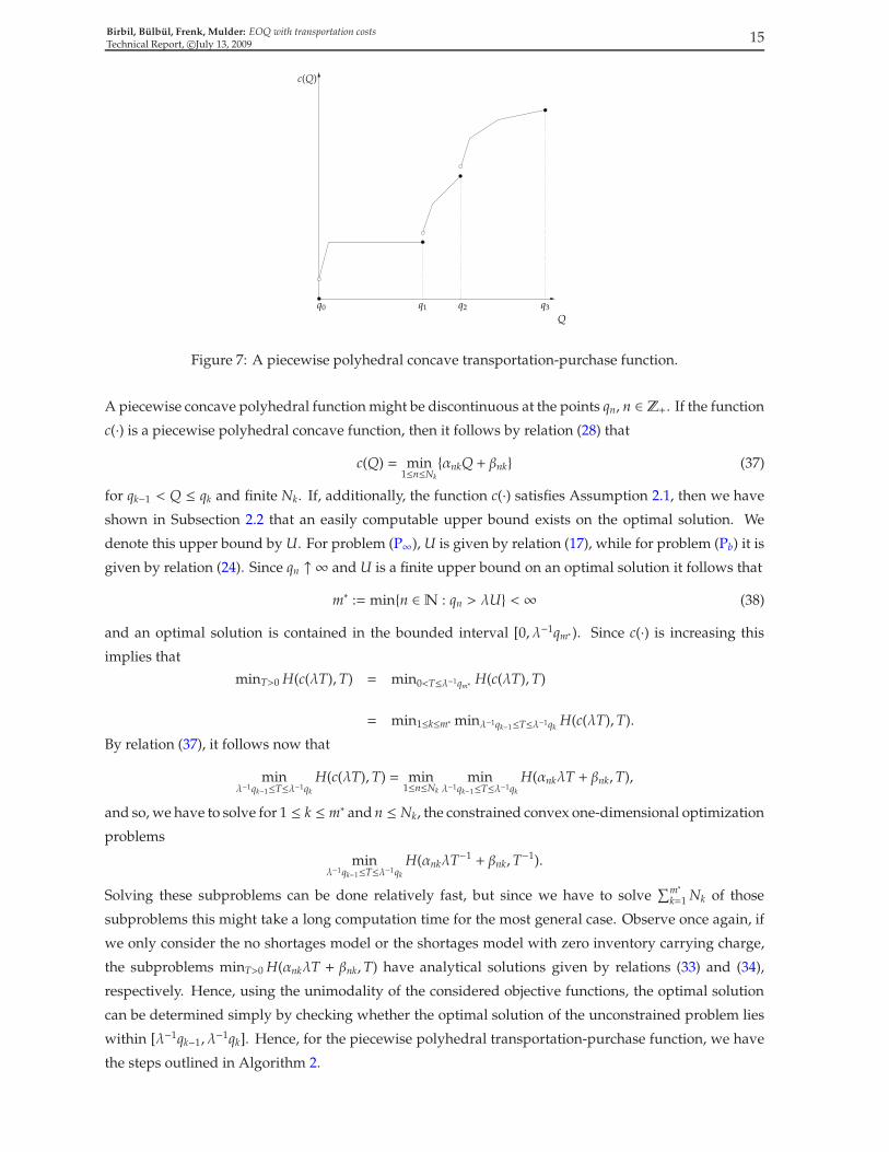
Example 3.1 (Carload Discount ScheduleWith Identical Trucks) Let C > 0 be the truck capacity, g :
(0,C] → R be an increasing polyhedral concave function satisfying g(0) = 0 and s ≥ 0 be the setup cost of
using one truck. Here, g(Q) corresponds to the transportation cost for transporting an order of size Q with
0 < Q ≤ C. If no discount is given on the number of used (identical) trucks, then the total transportation cost
function t : [0,∞)→ R has the form
t(Q) =
0, if Q = 0;
g(Q) + s, if 0 < Q ≤ C,
and
t(Q) = ng(C) + g(Q − nC) + (n + 1)s
for nC < Q ≤ (n + 1)C with integer n ≥ 1. Clearly, the above transportation function t(·) belongs to the class of
piecewise polyhedral concave functions with qn = nC. When we use the above transportation function t(·) with a
linear purchase function p(·), then we obtain a transportation-function c(·) similar to the one shown in Figure 8.
c(Q)
C 2C 3CQ
s
s
s
Figure 8: A transportation-purchase function for carload discount schedule with identical trucks.
Birbil, Bulbul, Frenk, Mulder: EOQ with transportation costsTechnical Report, c©July 13, 2009
17
For this class of functions it follows t(Q) ≥ t1(Q) for every Q ≥ 0 with
t1(Q) :=g(C) + s
CQ
and for dn := λ−1nC the equality
t(λdn) = t1(λdn)
holds for every n ∈ Z+. If the price of each ordered item equals π > 0 (no quantity discount), and hence the
purchase function p : [0,∞)→ R is given by p(Q) = πQ, it follows that the lower bounding function c1(·) of the
transportation-purchase function c(Q) = t(Q) + p(Q) is given by
c1(Q) = t1(Q) + p(Q) =
(
g(C) + s
C+ π
)
Q
and
c(λdn) = c1(λdn)
for every n ∈ Z+. Adding a linear function p(·) to the piecewise polyhedral concave function t(·) yields that
c(·) is a piecewise polyhedral concave function (see also Figure 8). Since for the EOQ-type model with linear
function c1(·) both the no shortages objective function T 7→ G(c1(λT),T) and the shortages objective function
T 7→ F(c1(λT),T) are unimodal, it follows by Lemma 2.2 that an optimal solution of the EOQ-type model with
transportation-purchase function c(·) is contained within the interval [dn∗ , dn∗+1] with
n∗ := max{n ∈ Z+ : dn ≤ Topt}, (39)
where Topt is the optimal solution of the EOQ-type model with linear transportation-purchase function c1(·). Since
dn = λ−1nC, this implies
n∗ = bλToptC−1c, (40)
where b·c denotes the floor function. In particular, if we consider the no shortages case (b = ∞), then we obtain
using relation (33) that the optimal solution Topt of the EOQ-type model with function c1(·) has an easy analytical
form given by
Topt =2
√
2a
λ(h + rp + r(g(C) + s)C−1). (41)
Likewise, for the EOQ-model with shortages (b < ∞) and no inventory carrying charge (r = 0), we obtain using
relation (34) that
Topt =2
√
2a(h + b)
λhb. (42)
Finally, for the most general EOQ-type model with shortages allowed and positive inventory carrying charge r,
there exists a fast algorithm to compute its optimal solution Topt. If Topt equals dn∗ or equivalently Topt is an integer
multiple of λ−1C the optimal solution of the EOQ model with function c(·) also equals Topt. Otherwise, as already
observed, the optimal solution of this EOQ model with function c(·) can be found in the interval (dn∗ , dn∗+1], and
so, we have to solve in the second step the optimization problem
mindn∗<T≤dn∗+1H(c(λT),T).
Algorithm 3 gives the details of solving the carload discount schedule with identical trucks.
When we generalize Example 3.1 to nonidentical trucks, we can use our results given for arbitrary
piecewise polyhedral concave functions. If we further concentrate on the carload discount schedule

18 Birbil, Bulbul, Frenk, Mulder: EOQ with transportation costsTechnical Report, c©July 13, 2009
Algorithm 3: Finding Topt for carload discount schedule with identical trucks
T∗ = arg minT>0 H(c1(λT),T)1:
if T∗ is not an integer multiple of λ−1C then2:
n∗ = bλToptC−1c3:
T∗ = arg mindn∗<T≤dn∗+1 H(c(λT),T)4:
Topt ← T∗5:
with nonincreasing truck setup costs as shown in Figure 9, then the lower lower bounding function c1(·)becomes polyhedral concave. In this case, we can develop a faster algorithm. To obtain a polyhedral
concave c1(·), we assume for n ≥ 1 that the sequence
δn :=c(qn) − c(qn−1)
qn − qn−1
is decreasing. Then, the function c1 : [0,∞)→ R becomes
c1(Q) = c(qn−1) + δn(Q − qn−1) = δnQ + γn (43)
for qn−1 ≤ Q ≤ qn, n ≥ 1 with γn = c(qn−1) − δnqn−1. As shown in Figure 9, c(qn) = c1(qn), n ∈ N, and
c(Q) ≥ c1(Q) for every Q ≥ 0.
γ1
γ2
γ3δ2
δ3
δ1
c(Q)
Qq0 q1 q2 q3
c1(Q)
Figure 9: A transportation-purchase function for carload discount schedule with nonincreasing truck
setup costs.
Since by construction c(Q) ≥ c1(Q) it follows that
H(c(λT),T) ≥ H(c1(λT),T).
We will now show by means of the concavity of the lower bounding function c1(·) that one can determine
a better upper bound than (38). We know for any d belonging to the set
Dζ = {d > 0 : c1(λd) ≤ hλd2ζ
2− a}
that
H(c1(λT),T) ≥ H(c1(λd), d) (44)

Birbil, Bulbul, Frenk, Mulder: EOQ with transportation costsTechnical Report, c©July 13, 2009
19
for any T ≥ d. By the concavity of c1(·), this implies for
n∗ := max{n ∈N : c1(qn) >hqn
2ζ
2λ− a}
that
H(c1(λT),T) ≥ H(c1(qn∗+1), λ−1qn∗+1) (45)
for every T ≥ λ−1qn∗+1. This implies by relation (44) and c(qn∗+1) = c1(qn∗+1) that
H(c(λT),T) ≥ H(c(qn∗+1), λ−1qn∗+1)
for every T ≥ λ−1qn∗+1. Hence we have shown that any optimal solution of the original EOQ model
with transportation-purchase function c(·) is contained in [0,λ−1qn∗+1]. By the discussion at the end
of Subsection 2.2 and relation (38), it follows that n∗ ≤ m∗ and this shows that the newly constructed
upper bound is at least as good as the constructed bound for an arbitrary piecewise polyhedral concave
function. Therefore, the number of subproblems to be solved could be far less than m∗. We investigate
this issue in the next section.
4. Computational Study. We designed our numerical experiments with two basic goals in mind.
First, we would like to demonstrate that the EOQ model is amenable to fast solution methods in the
presence of a general class of transportation functions introduced in this paper. Second, we aim to
shed some light into the dynamics of the EOQ model under the carload discount schedule which seems
to be the most well-known transportation function in the literature. Recall that in our analysis we
assumed that there exists an affine upper bound on the transportation-purchase function (Assumption
2.1). Though straightforward, for completeness we explicitly give in Appendix B the steps to compute
these affine bounds for the functions that are used in our computational experiments.
The algorithms we developed were implemented in Matlab R2008a, and the numerical experiments
were performed on a Lenovo T400 portable computer with an Intel Centrino 2 T9400 processor and 4GB
of memory.
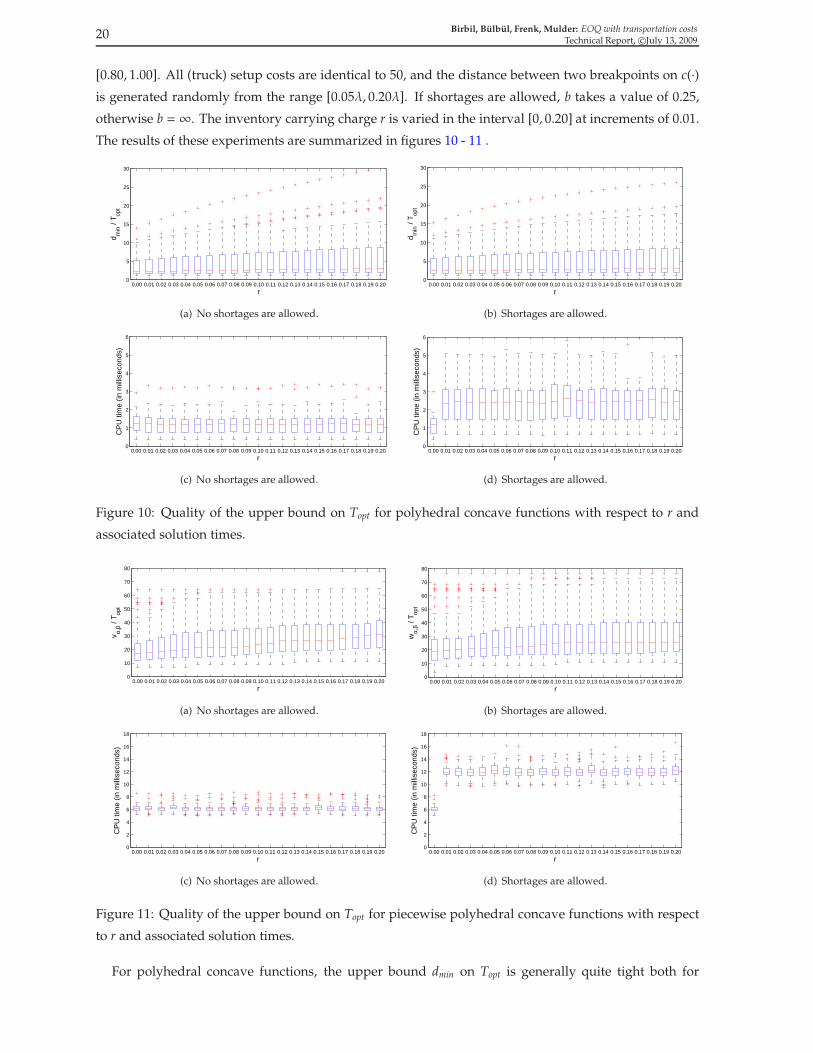
4.1 Tightness of The Upper Bounds on Topt for Polyhedral Concave and Piecewise Polyhedral
Concave c(·). In the final paragraph of Example 2.1, we reckoned that the constructed upper bound
vα,β on dmin given in (17) for the no shortages case may be weak for problems with strictly positive
inventory carrying charge r because vα,β does not contain the value of r. The same is true for the upper
bound wα,β on dmin defined in (24) if shortages are allowed. Thus, in the first part of our computational
study we explore the strength of the upper bounds on Topt as r changes. To this end, 100 instances
are created and solved for varying values of r for both polyhedral concave and piecewise polyhedral
concave transportation-purchase functions. For all of these instances, we set λ = 1500, a = 200, h = 0.05.
Piecewise polyhedral concave functions consist of 20 intervals over which the transportation-purchase
function c(·) is polyhedral concave. In this case, each polyhedral concave function is constructed by the
minimum of a number of affine functions where this number is chosen randomly from the range [2, 5].
If c(·) is polyhedral concave on [0,∞), then the number of linear pieces on c(·) is selected randomly from
the range [2, 20]. For both piecewise polyhedral concave and polyhedral concave c(·), the slope of the
first affine function on each polyhedral concave function is distributed as U[0.50, 1.00]. The following
slopes are calculated by multiplying the immediately preceding slope by a random number in the range
20 Birbil, Bulbul, Frenk, Mulder: EOQ with transportation costsTechnical Report, c©July 13, 2009
[0.80, 1.00]. All (truck) setup costs are identical to 50, and the distance between two breakpoints on c(·)is generated randomly from the range [0.05λ, 0.20λ]. If shortages are allowed, b takes a value of 0.25,
otherwise b = ∞. The inventory carrying charge r is varied in the interval [0, 0.20] at increments of 0.01.
The results of these experiments are summarized in figures 10 - 11 .
0.00 0.01 0.02 0.03 0.04 0.05 0.06 0.07 0.08 0.09 0.10 0.11 0.12 0.13 0.14 0.15 0.16 0.17 0.18 0.19 0.200
5
10
15
20
25
30
d min
/ T op
t
r
(a) No shortages are allowed.
0.00 0.01 0.02 0.03 0.04 0.05 0.06 0.07 0.08 0.09 0.10 0.11 0.12 0.13 0.14 0.15 0.16 0.17 0.18 0.19 0.200
5
10
15
20
25
30
d min
/ T op
t
r
(b) Shortages are allowed.
0.00 0.01 0.02 0.03 0.04 0.05 0.06 0.07 0.08 0.09 0.10 0.11 0.12 0.13 0.14 0.15 0.16 0.17 0.18 0.19 0.200
1
2
3
4
5
6
CP
U ti
me
(in m
illis
econ
ds)
r
(c) No shortages are allowed.
0.00 0.01 0.02 0.03 0.04 0.05 0.06 0.07 0.08 0.09 0.10 0.11 0.12 0.13 0.14 0.15 0.16 0.17 0.18 0.19 0.200
1
2
3
4
5
6
CP
U ti
me
(in m
illis
econ
ds)
r
(d) Shortages are allowed.
Figure 10: Quality of the upper bound on Topt for polyhedral concave functions with respect to r and
associated solution times.
0.00 0.01 0.02 0.03 0.04 0.05 0.06 0.07 0.08 0.09 0.10 0.11 0.12 0.13 0.14 0.15 0.16 0.17 0.18 0.19 0.200
10
20
30
40
50
60
70
80
v α,β /
T opt
r
(a) No shortages are allowed.
0.00 0.01 0.02 0.03 0.04 0.05 0.06 0.07 0.08 0.09 0.10 0.11 0.12 0.13 0.14 0.15 0.16 0.17 0.18 0.19 0.200
10
20
30
40
50
60
70
80
wα,
β / T op
t
r
(b) Shortages are allowed.
0.00 0.01 0.02 0.03 0.04 0.05 0.06 0.07 0.08 0.09 0.10 0.11 0.12 0.13 0.14 0.15 0.16 0.17 0.18 0.19 0.200
2
4
6
8
10
12
14
16
18
CP
U ti
me
(in m
illis
econ
ds)
r
(c) No shortages are allowed.
0.00 0.01 0.02 0.03 0.04 0.05 0.06 0.07 0.08 0.09 0.10 0.11 0.12 0.13 0.14 0.15 0.16 0.17 0.18 0.19 0.200
2
4
6
8
10
12
14
16
18
CP
U ti
me
(in m
illis
econ
ds)
r
(d) Shortages are allowed.
Figure 11: Quality of the upper bound on Topt for piecewise polyhedral concave functions with respect
to r and associated solution times.
For polyhedral concave functions, the upper bound dmin on Topt is generally quite tight both for
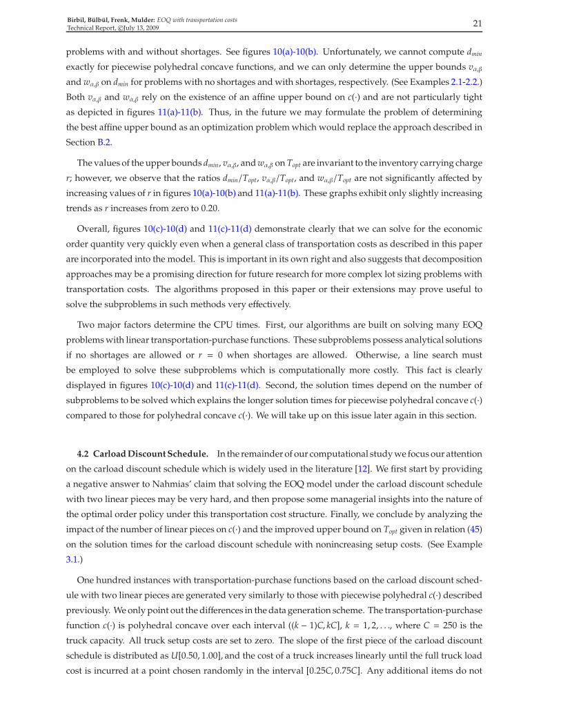
Birbil, Bulbul, Frenk, Mulder: EOQ with transportation costsTechnical Report, c©July 13, 2009
21
problems with and without shortages. See figures 10(a)-10(b). Unfortunately, we cannot compute dmin
exactly for piecewise polyhedral concave functions, and we can only determine the upper bounds vα,β
and wα,β on dmin for problems with no shortages and with shortages, respectively. (See Examples 2.1-2.2.)
Both vα,β and wα,β rely on the existence of an affine upper bound on c(·) and are not particularly tight
as depicted in figures 11(a)-11(b). Thus, in the future we may formulate the problem of determining
the best affine upper bound as an optimization problem which would replace the approach described in
Section B.2.
The values of the upper bounds dmin, vα,β, and wα,β on Topt are invariant to the inventory carrying charge
r; however, we observe that the ratios dmin/Topt, vα,β/Topt, and wα,β/Topt are not significantly affected by
increasing values of r in figures 10(a)-10(b) and 11(a)-11(b). These graphs exhibit only slightly increasing
trends as r increases from zero to 0.20.
Overall, figures 10(c)-10(d) and 11(c)-11(d) demonstrate clearly that we can solve for the economic
order quantity very quickly even when a general class of transportation costs as described in this paper
are incorporated into the model. This is important in its own right and also suggests that decomposition
approaches may be a promising direction for future research for more complex lot sizing problems with
transportation costs. The algorithms proposed in this paper or their extensions may prove useful to
solve the subproblems in such methods very effectively.
Two major factors determine the CPU times. First, our algorithms are built on solving many EOQ
problems with linear transportation-purchase functions. These subproblems possess analytical solutions
if no shortages are allowed or r = 0 when shortages are allowed. Otherwise, a line search must
be employed to solve these subproblems which is computationally more costly. This fact is clearly
displayed in figures 10(c)-10(d) and 11(c)-11(d). Second, the solution times depend on the number of
subproblems to be solved which explains the longer solution times for piecewise polyhedral concave c(·)compared to those for polyhedral concave c(·). We will take up on this issue later again in this section.
4.2 Carload Discount Schedule. In the remainder of our computational study we focus our attention
on the carload discount schedule which is widely used in the literature [12]. We first start by providing
a negative answer to Nahmias’ claim that solving the EOQ model under the carload discount schedule
with two linear pieces may be very hard, and then propose some managerial insights into the nature of
the optimal order policy under this transportation cost structure. Finally, we conclude by analyzing the
impact of the number of linear pieces on c(·) and the improved upper bound on Topt given in relation (45)
on the solution times for the carload discount schedule with nonincreasing setup costs. (See Example
3.1.)
One hundred instances with transportation-purchase functions based on the carload discount sched-
ule with two linear pieces are generated very similarly to those with piecewise polyhedral c(·) described
previously. We only point out the differences in the data generation scheme. The transportation-purchase
function c(·) is polyhedral concave over each interval ((k − 1)C, kC], k = 1, 2, . . ., where C = 250 is the
truck capacity. All truck setup costs are set to zero. The slope of the first piece of the carload discount
schedule is distributed as U[0.50, 1.00], and the cost of a truck increases linearly until the full truck load
cost is incurred at a point chosen randomly in the interval [0.25C, 0.75C]. Any additional items do not
22 Birbil, Bulbul, Frenk, Mulder: EOQ with transportation costsTechnical Report, c©July 13, 2009
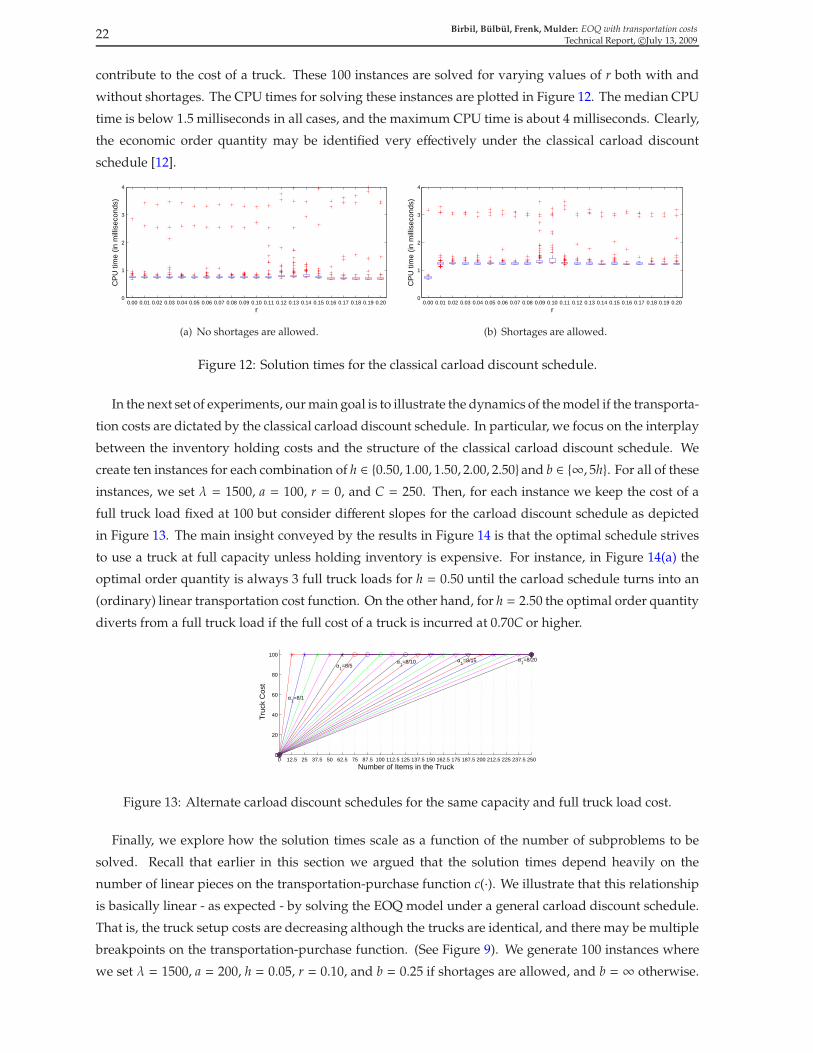
contribute to the cost of a truck. These 100 instances are solved for varying values of r both with and
without shortages. The CPU times for solving these instances are plotted in Figure 12. The median CPU
time is below 1.5 milliseconds in all cases, and the maximum CPU time is about 4 milliseconds. Clearly,
the economic order quantity may be identified very effectively under the classical carload discount
schedule [12].
0.00 0.01 0.02 0.03 0.04 0.05 0.06 0.07 0.08 0.09 0.10 0.11 0.12 0.13 0.14 0.15 0.16 0.17 0.18 0.19 0.200
1
2
3
4
CP
U ti
me
(in m
illis
econ
ds)
r
(a) No shortages are allowed.
0.00 0.01 0.02 0.03 0.04 0.05 0.06 0.07 0.08 0.09 0.10 0.11 0.12 0.13 0.14 0.15 0.16 0.17 0.18 0.19 0.200
1
2
3
4
CP
U ti
me
(in m
illis
econ
ds)
r
(b) Shortages are allowed.
Figure 12: Solution times for the classical carload discount schedule.
In the next set of experiments, our main goal is to illustrate the dynamics of the model if the transporta-
tion costs are dictated by the classical carload discount schedule. In particular, we focus on the interplay
between the inventory holding costs and the structure of the classical carload discount schedule. We
create ten instances for each combination of h ∈ {0.50, 1.00, 1.50, 2.00, 2.50}and b ∈ {∞, 5h}. For all of these
instances, we set λ = 1500, a = 100, r = 0, and C = 250. Then, for each instance we keep the cost of a
full truck load fixed at 100 but consider different slopes for the carload discount schedule as depicted
in Figure 13. The main insight conveyed by the results in Figure 14 is that the optimal schedule strives
to use a truck at full capacity unless holding inventory is expensive. For instance, in Figure 14(a) the
optimal order quantity is always 3 full truck loads for h = 0.50 until the carload schedule turns into an
(ordinary) linear transportation cost function. On the other hand, for h = 2.50 the optimal order quantity
diverts from a full truck load if the full cost of a truck is incurred at 0.70C or higher.
0 12.5 25 37.5 50 62.5 75 87.5 100 112.5 125 137.5 150 162.5 175 187.5 200 212.5 225 237.5 2500
20
40
60
80
100
α1=8/1
α1=8/5
α1=8/10 α
1=8/15 α
1=8/20
Number of Items in the Truck
Tru
ck C
ost
Figure 13: Alternate carload discount schedules for the same capacity and full truck load cost.
Finally, we explore how the solution times scale as a function of the number of subproblems to be
solved. Recall that earlier in this section we argued that the solution times depend heavily on the
number of linear pieces on the transportation-purchase function c(·). We illustrate that this relationship
is basically linear - as expected - by solving the EOQ model under a general carload discount schedule.
That is, the truck setup costs are decreasing although the trucks are identical, and there may be multiple
breakpoints on the transportation-purchase function. (See Figure 9). We generate 100 instances where
we set λ = 1500, a = 200, h = 0.05, r = 0.10, and b = 0.25 if shortages are allowed, and b = ∞ otherwise.
Birbil, Bulbul, Frenk, Mulder: EOQ with transportation costsTechnical Report, c©July 13, 2009
23
0 0.05 0.1 0.15 0.2 0.25 0.3 0.35 0.4 0.45 0.5 0.55 0.6 0.65 0.7 0.75 0.8 0.85 0.9 0.95 10
0.05
0.1
0.15
0.2
0.25
0.3
0.35
0.4
0.45
0.5
0.55
0.6
Full Truck Cost Incurred at (Expressed As a Fraction of Truck Capacity C)
Top
t
h=0.50h=1.00h=1.50h=2.00h=2.50
(a) No shortages are allowed.
0 0.05 0.1 0.15 0.2 0.25 0.3 0.35 0.4 0.45 0.5 0.55 0.6 0.65 0.7 0.75 0.8 0.85 0.9 0.95 10
0.05
0.1
0.15
0.2
0.25
0.3
0.35
0.4
0.45
0.5
0.55
0.6
Full Truck Cost Incurred at (Expressed As a Fraction of Truck Capacity C)
Top
t
h=0.50h=1.00h=1.50h=2.00h=2.50
(b) Shortages are allowed.
0 0.05 0.1 0.15 0.2 0.25 0.3 0.35 0.4 0.45 0.5 0.55 0.6 0.65 0.7 0.75 0.8 0.85 0.9 0.95 1950
1000
1050
1100
1150
1200
1250
1300
1350
1400
1450
1500
1550
Full Truck Cost Incurred at (Expressed As a Fraction of Truck Capacity C)
Tot
al C
ost
h=0.50h=1.00h=1.50h=2.00h=2.50
(c) No shortages are allowed.
0 0.05 0.1 0.15 0.2 0.25 0.3 0.35 0.4 0.45 0.5 0.55 0.6 0.65 0.7 0.75 0.8 0.85 0.9 0.95 1950
1000
1050
1100
1150
1200
1250
1300
1350
1400
1450
1500
1550
Full Truck Cost Incurred at (Expressed As a Fraction of Truck Capacity C)
Tot
al C
ost
h=0.50h=1.00h=1.50h=2.00h=2.50
(d) Shortages are allowed.
Figure 14: Optimal cycle length and cost for alternate carload discount schedules and different h values.
As before, the truck capacity is C = 250, and the transportation-purchase function c(·) is polyhedral
concave over each interval ((k − 1)C, kC], k = 1, 2, . . .. The setup cost of the first truck is distributed as
U[50, 100], and for each following truck the setup cost is computed by multiplying that of the previous
truck with a random number in the range [0.50, 1.00]. For each truck, the number of breakpoints on
the discount schedule is created randomly in the range [2, 20], and the distance between two successive
breakpoints is calculated by multiplying the remaining capacity of the truck by a random number in
[0.05, 0.20]. The slope of the first linear piece is distributed as U[0.50, 1.00] and subsequent slopes are
obtained by multiplying the slopes of the immediately preceding pieces by a random number in the
range [0.80, 1.00]. The final slope is always zero. In Figure 15, we plot the solution times against the
number of subproblems solved and conclude that the relationship between these two quantities is linear.
The dotted lines in the figure are fitted by simple linear regression through the origin. We also observe
that the relatively tighter upper bound on Topt given in relation (45) for carload discount schedules with
nonincreasing setup costs provides computational savings of 22% and 28% on average for instances with
and without shortages, respectively.

24 Birbil, Bulbul, Frenk, Mulder: EOQ with transportation costsTechnical Report, c©July 13, 2009
0 500 1000 1500 2000 2500 3000 3500 4000 45000
100
200
300
400
500
600
Number of Linear Pieces on the Transportation−Purchase Function
CP
U T
ime
(in m
illis
econ
ds)
Based on m*
Based on n*
(a) No shortages are allowed.
0 500 1000 1500 2000 2500 3000 3500 4000 45000
100
200
300
400
500
600
Number of Linear Pieces on the Transportation−Purchase Function
CP
U T
ime
(in m
illis
econ
ds)
Based on m*
Based on n*
(b) Shortages are allowed.
Figure 15: Solution times for the carload discount schedule with nonincreasing setup costs and multiple
linear pieces.
Birbil, Bulbul, Frenk, Mulder: EOQ with transportation costsTechnical Report, c©July 13, 2009
25
5. Conclusion and Future Research. In this work, we have analyzed the impact of the transportation
cost in EOQ-type models. We investigated the structures of the resulting problems and derived bounds
on their optimal cycle lengths. Observing that the carload discount schedule is frequently used in
the real practice, we have identified a subclass of problems that also includes the well-known carload
discount schedule. Due to their special structure, we have shown that the problems within this class are
relatively easy to solve. Using our analysis, we have also laid down the steps of several fast algorithms.
To support our analysis and results, we have setup a thorough computational study and discussed our
observations from different angles. Overall, we have concluded that a large group of EOQ-type problems
with transportation costs can be considered as simple problems and they can be solved very efficiently
in almost no time. In the future, we intend to study the extension of the EOQ-type problems to stochastic
single item inventory models with arbitrary transportation costs.
Acknowledgments. We would like to acknowledge The Scientific and Technological Research Coun-
cil of Turkey (TUBITAK) for their support under grant 2221.
26 Birbil, Bulbul, Frenk, Mulder: EOQ with transportation costsTechnical Report, c©July 13, 2009
Appendix A. Existence Result. In this appendix we show that the optimization problem (P) with
H(·, ·) belonging toH and c(·) an increasing left continuous function has an optimal solution.
Definition A.1 A function f : [0,∞)→ R is called lower semi-continuous at x ≥ 0 if
lim infk↑∞ f (xk) ≥ f (x)
for every sequence xk satisfying limk↑∞ xk = x. The function is called lower semi-continuous if it is lower semi-
continuous at every x ≥ 0.
It is well known (see for example [13] or [6]) that the function f : [0,∞)→ R is lower semi-continuous
if and only if for every α ∈ R the lower level set
L(α) = {x ∈ [0,∞) : f (x) ≤ α}
is closed. It is now possible to show the next result. Observe we extend the EOQ-type function
T 7→ H(c(T),T) defined on (0,∞) to [0,∞) by defining H(c(0), 0) = ∞.
Lemma A.1 If c(·) is an increasing left continuous function and H belongs to H (·, ·), then the function T 7→H(c(T),T) is lower semi-continuous on [0,∞).
Proof. By the previous remark we have to show that the lower level set L(α) := {T ∈ [0,∞) :
H(c(T),T) ≤ α} is closed for every α ∈ R. Let α ∈ R be given and consider some sequence (Tn)n∈N ⊆ L(α)
satisfying limk↑∞ Tk = T. Consider now the following two mutually exclusive cases. If there exists an
infinite setN0 ⊆N satisfying T ≤ Tn for every n ∈ N0, then by the monotonicity of c it follows c(T) ≤ c(Tn)
for every n ∈ N0. This implies by the monotonicity of the function x 7→ H(x,T) for every T > 0 that
H(c(T),Tn) ≤ H(c(Tn),Tn) ≤ α
for every n ∈ N0. Since N0 is an infinite set and limn∈N0↑∞ Tn = T we obtain by the continuity of
x 7→ H(c(T), x) that
H(c(T),T) = limn∈N0↑∞H(c(T),Tn) ≤ α.
If there does not exist an infinite setN0 ⊆N satisfying T ≤ Tn for every n ∈ N0, then clearly one can find
a strictly increasing sequence (Tn)n∈N1satisfying limn∈N1
Tn ↑ T. This implies by the left continuity of c
that limn∈N1c(Tn) = c(T) and applying now the continuity of H it follows
α ≥ limn∈N1H(c(Tn),Tn) = H(c(T),T)
Hence for both cases we have shown that H(c(T),T) ≤ α and so L(α) is closed. �
By Lemma A.1 and H(·, ·) belonging toH implying
limT↓0 H(x,T) = limT↑∞H(x,T) = ∞
for every x ≥ 0 we obtain by the Weierstrass-Lebesgue lemma [1] that the optimization problem (P) has
an optimal solution.
Birbil, Bulbul, Frenk, Mulder: EOQ with transportation costsTechnical Report, c©July 13, 2009
27
Appendix B. Computing The Affine Upper Bounds. In this appendix, we demonstrate how an
affine function may be computed that satisfies (11) for both the carload discount schedule and the
piecewise polyhedral concave transportation-purchase functions.
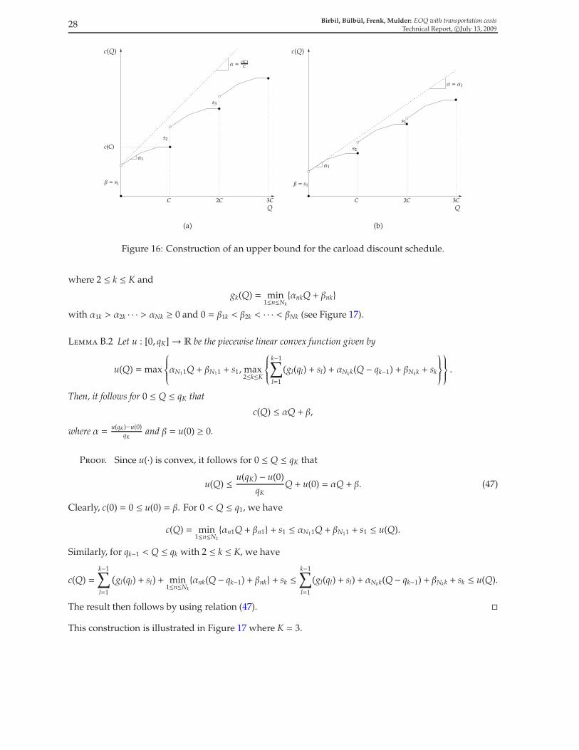
B.1 The Carload Schedule. Without loss of generality, we only consider carload discount schedules
with nonincreasing truck setup costs which also includes trucks with identical setup costs as a special
case. Similar to the construction in Example 3.1, we let g : (0,C] → R be an increasing polyhedral
concave function satisfying g(0) = 0 and si with si ≥ si−1 ≥ 0, i ≥ 1 be the setup cost of the ith truck. We
then define
c(Q) =
0, if Q = 0;
g(Q) + s1, if 0 < Q ≤ C,
where
g(Q) = min1≤k≤N
{αkQ + βk} (46)
with α1 > α2 > · · · > αN ≥ 0 and 0 = β1 < β2 < · · · < βN, and
c(Q) =
n+1∑
i=1
si + ng(C) + g(Q − nC)
for nC < Q ≤ (n + 1)C with integer n ≥ 1 (see Figure 16).
Lemma B.1 For a discount carload schedule with nonincreasing setup costs si ≥ 0, i ≥ 1 it follows that
c(Q) ≤ αQ + β,
where α = max(α1, c(C)C−1) and β = s1.
Proof. Since s1 ≥ 0, we have c(0) = 0 ≤ s1 = β. For 0 < Q ≤ C, it follows by relation (46) that
c(Q) = min1≤k≤N
{αkQ + βk} + s1 ≤ α1Q + s1 ≤ max(α1, c(C)C−1)Q + s1 = αQ + β.
For nC < Q ≤ (n + 1)C with integer n ≥ 1, we have
c(Q) =∑n+1
i=1 si + ng(C) + g(Q − nC) ≤ (n + 1)s1 + ng(C) + g(Q − nC)
= n(s1 + g(C)) + g(Q − nC) + s1
= nc(C) + g(Q − nC) + s1
≤ max(α1, c(C)C−1)nC +min1≤k≤N{αk(Q − nC) + βk} + s1
≤ max(α1, c(C)C−1)nC + α1(Q − nC) + s1
≤ max(α1, c(C)C−1)Q + s1
= αQ + β.
�
B.2 Piecewise Polyhedral Concave Functions. We next compute an affine bound for a piecewise
polyhedral concave function over the predefined interval [0, qK], where K corresponds to the number
of trucks under consideration. Let gk : (qk−1, qk] → R be an increasing polyhedral concave function
satisfying gk(0) = 0 and si ≥ 0 be the setup cost of the ith truck. We then define
c(Q) =
0, if Q = 0;
g1(Q) + s1, if 0 < Q ≤ q1;∑k−1
l=1
(
gl(ql) + sl)
+ gk(Q − qk−1) + sk, if qk−1 < Q ≤ qk,
28 Birbil, Bulbul, Frenk, Mulder: EOQ with transportation costsTechnical Report, c©July 13, 2009
Q
c(Q)
α =c(C)
C
s2
s3
c(C)
β = s1
α1
C 2C 3C
(a)
c(Q)
Q
α = α1
s3
α1
C 2C 3C
s2
β = s1
(b)
Figure 16: Construction of an upper bound for the carload discount schedule.
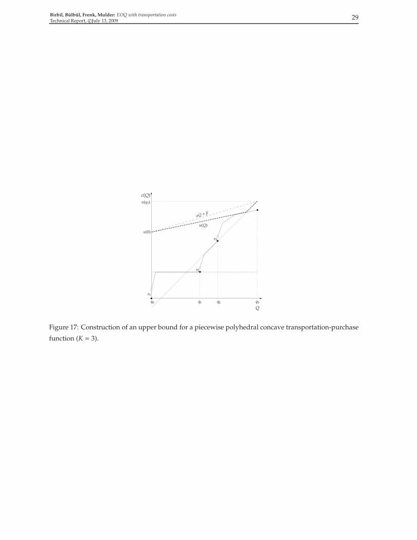
where 2 ≤ k ≤ K and
gk(Q) = min1≤n≤Nk
{αnkQ + βnk}
with α1k > α2k · · · > αNk ≥ 0 and 0 = β1k < β2k < · · · < βNk (see Figure 17).
Lemma B.2 Let u : [0, qK]→ R be the piecewise linear convex function given by
u(Q) = max
αN11Q + βN11 + s1,max2≤k≤K
k−1∑
l=1
(gl(ql) + sl) + αNkk(Q − qk−1) + βNkk + sk
.
Then, it follows for 0 ≤ Q ≤ qK that
c(Q) ≤ αQ + β,
where α =u(qK)−u(0)
qKand β = u(0) ≥ 0.
Proof. Since u(·) is convex, it follows for 0 ≤ Q ≤ qK that
u(Q) ≤u(qK) − u(0)
qKQ + u(0) = αQ + β. (47)
Clearly, c(0) = 0 ≤ u(0) = β. For 0 < Q ≤ q1, we have
c(Q) = min1≤n≤N1
{αn1Q + βn1} + s1 ≤ αN11Q + βN11 + s1 ≤ u(Q).
Similarly, for qk−1 < Q ≤ qk with 2 ≤ k ≤ K, we have
c(Q) =
k−1∑
l=1
(
gl(ql) + sl)
+ min1≤n≤Nk
{αnk(Q− qk−1) + βnk} + sk ≤k−1∑
l=1
(gl(ql) + sl) + αNkk(Q− qk−1) + βNkk + sk ≤ u(Q).
The result then follows by using relation (47). �
This construction is illustrated in Figure 17 where K = 3.
Birbil, Bulbul, Frenk, Mulder: EOQ with transportation costsTechnical Report, c©July 13, 2009
29
q0 q1 q2 q3
Q
c(Q)
u(Q)
αQ + β
u(q3)
s2
u(0)
s3
s1
Figure 17: Construction of an upper bound for a piecewise polyhedral concave transportation-purchase
function (K = 3).

30 Birbil, Bulbul, Frenk, Mulder: EOQ with transportation costsTechnical Report, c©July 13, 2009
References
[1] Aubin, J.B. Optima and Equilibra (An introduction to nonlinear analysis), volume 140 of Graduate Texts
in Mathematics. Springer Verlag, Berlin, 1993.
[2] Bayındır, Z.P., Birbil, S.I and J.B.G., Frenk. The joint replenishment problem with variable production
costs. European Journal of Operational Research, 175(1):622–640, 2006.
[3] Bazaraa, M.S., Sherali, H.D. and C.M. Shetty. Nonlinear Programming: Theory and Algorithms (second
edition). Wiley, New York, 1993.
[4] Bector, C.R. Programming problems with convex fractional functions. Operations Research, 16(2):383–
391, 1968.
[5] Carter, J.R and B.G. Ferrin. Transportation costs and inventory management: Why transportation
costs matter. Production and Inventory Management Journal, 37(3):58–62, 1996.
[6] Frenk, J.B.G. and G. Kassay. Introduction to convex and quasiconvex analysis. In Hadjisav-
vas, N., Komlosi, S. and S. Schaible, editor, Handbook of Generalized Convexity and Generalized Mono-
tonicity, pages 3–87. Springer, Dordrecht, 2005.
[7] Hadley, G. and T.M. Whitin. Analysis of Inventory Systems. Prentice Hall, Englewood Cliffs, 1963.
[8] Harris, F.W. How many parts to make at once. Factory, The Magazine of Management, 10(2):135–136,
1913.
[9] Hiriart-Urruty, J.B. and C. Lemarechal. Convex Analysis and Minimization Algorithms, volume 1.
Springer Verlag, Berlin, 1993.
[10] Horst, R., Pardalos, P.M. and N.V. Thoai. Introduction to Global Optimization. Kluwer Academic
Publishers, Dordrecht, 1995.
[11] Lee, C. The economic order quantity for freight discount costs. IIE Transactions, 18(3):318–320, 1986.
[12] Nahmias, S. Production and Operations Analysis (third edition). Irwin/McGraw-Hill, New York, 1997.
[13] Rockafellar, R.T. Convex Analysis. Princeton University Press, New Jersey, 1972.
[14] Zipkin, P.H. Foundations of Inventory Management. McGraw-Hill, New York, 2000.


![TROXLER TRANSPORTATION GUIDE - … offered by Troxler) Transportation Guide 3. ... and quantity of radioactive material in most Troxler nuclear ... [§172.403(g)]: Contents – the](https://img.pdfslide.us/doc/110x75/5b3e76e77f8b9a0e628eec1b/troxler-transportation-guide-offered-by-troxler-transportation-guide-3-and.jpg)