On the dynamic control of matching queues

Itai GurvichNorthwestern University

i-gurvich@northwestern.edu

Amy WardUniversity of Southern Californiaamyward@marshall.usc.edu

January 2013

Abstract

We consider the optimal control of matching queues with dynamically arriving jobs. In thismodel, jobs arrive to their dedicated queues, and wait to be matched with jobs from other(possibly many) queues. Given that all jobs in a match are present in the system, the matchingitself is instantaneous. The objective is to minimize cumulative job holding costs. In the specialcase of linear (and equal across classes) holding costs, this is equivalent to maximizing thenumber of matched jobs. The key control question is whether to match myopically, or to keep“inventory” of jobs, to facilitate more profitable matches in the future. Problems of holding costminimization have been well-studied in the processing networks literature, and, in the traditionalparallel server setting, MaxWeight scheduling policies and variants thereof have been proved toperform well. The heavy-traffic phenomena of state-space collapse and the ensuing reduction ofthe problem to a one-dimensional Brownian control problem (under appropriate resource poolingconditions), that are the drivers of these well-known results, do not hold in the matching queuesetting that we study here. This difference is driven by the fundamentally different notions ofcapacity underlying the two settings.

We introduce a multi-dimensional imbalance process, that at each time t, is given by a linearfunction of the cumulative arrivals to each of the job types. In essence, the imbalance at a time tcaptures the number of additional jobs required so that some control policy could have matchedall the jobs that have arrived by that time (thus leaving the queues empty). The imbalancefacilitates the construction of a lower bound that is specified, at each time point, by a solutionto a simple constrained optimization problem. Achieving this lower bound requires, in general,“re-shuffling” past matches. Under a so-called match-pooling condition, we are able to devisea discrete-review matching policy that asymptotically – as the arrival rates becomes large –achieves the imbalance-based lower bound. Our optimality results hold for both stationary andnon-stationary arrivals.

1 Introduction

We consider the matching of dynamically arriving jobs. Jobs of different types arrive sequentiallyaccording to a random process and wait in their respective queues – a queue for each type. Jobsleave the system only after they are matched to jobs of other types. Matchings can be pairwise(matching only two jobs) or include multiple jobs in which case they are referred to as chains. Onceseveral jobs are matched they leave the system together. We refer to such systems as matchingqueues and are concerned with their optimal control.

1

3 2 4

1

A B

λ2 λ3 λ1 λ4

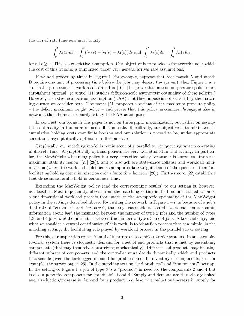
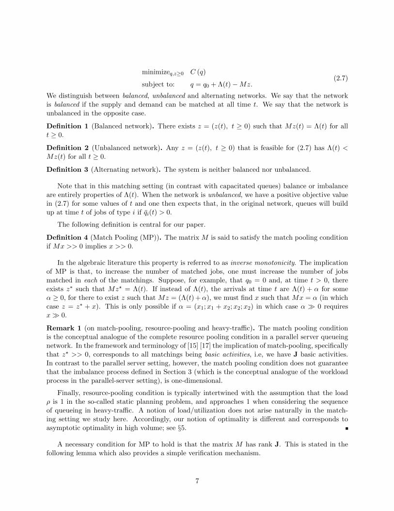
Figure 1: A network with four input streams and two matchings: (a) the chains view (b) a queueingnetwork view

In the example depicted in Figure 1, there are 4 types of jobs, and each type of job arrives inaccordance with a time-varying Poisson process having instantaneous rate λi(t), i = 1, 2, 3, 4. Jobsof type 1 can be matched to jobs of type 2. Jobs of type 2 can be matched with jobs of types 3and 4. When a type-1 job is matched with a type-2 job they both leave the system. A job of type4 must be matched to both a type-3 and a type-2 job to leave the system. The decision of thecontroller in such a network is when to perform a matching. There are clear tradeoffs underlyingthis decision. In Figure 1, suppose that there is a job available in each of the type-1, type-2 andtype-4 queues but none in the type-3 queue, one may be myopic and match the type-1 job withthe type-2 job. This would result in two jobs being matched and leaving the system. It may be,however, better to reserve some of the type-2 jobs and wait until a type-3 job arrives and match itwith a type-2 and type-4 jobs – depleting 3 jobs at once.

In the preceding example, type-2 jobs play the dual role of a “server” that is a resource for atype-1 job, and a “customer”, that is in need of a type-3 job. This is a fundamental observation thatis true of all job types. Its significance is that it is not possible to rapidly deplete one of the queues byfocusing processing resources on that queue, as is true in parallel server queueing systems that satisfya complete resource pooling condition (see, for example, [18], [31], and [22]). As a consequence,it is not straightforward to apply the “standard Brownian approximation methodology” proposedin [14] to find good control policies for the matching queue network. In particular, it is not clearwhat the so-called “workload process” is in the matching queue network.

A natural first question is to characterize the stability region for the network. For generalmatching models, this is known to be a very difficult question; see e.g. [9] and [8]. In our matchingsetting stability is not attainable and it is sensible instead to search for matching policies underwhich the build-up of jobs is minimal. In Figure 1, in order to avoid a significant build-up of jobs,

2

the arrival-rate functions must satisfy∫ t

0λ2(s)ds =

∫ t

0(λ1(s) + λ3(s) + λ4(s))ds and

∫ t

0λ3(s)ds =

∫ t

0λ4(s)ds,

for all t ≥ 0. This is a restrictive assumption. Our objective is to provide a framework under whichthe cost of this buildup is minimized under very general arrival rate assumptions.

If we add processing times in Figure 1 (for example, suppose that each match A and matchB require one unit of processing time before the jobs may depart the system), then Figure 1 is astochastic processing network as described in [16]. [10] prove that maximum pressure policies arethroughput optimal. (a sequel [11] studies diffusion-scale asymptotic optimality of these policies.)However, the extreme allocation assumption (EAA) that they impose is not satisfied by the match-ing queues we consider here. The paper [21] proposes a variant of the maximum pressure policy– the deficit maximum weight policy – and proves that this policy maximizes throughput also innetworks that do not necessarily satisfy the EAA assumption.

In contrast, our focus in this paper is not on throughput maximization, but rather on asymp-totic optimality in the more refined diffusion scale. Specifically, our objective is to minimize thecumulative holding costs over finite horizon and our solution is proved to be, under appropriateconditions, asymptotically optimal in diffusion scale.

Graphically, our matching model is reminiscent of a parallel server queueing system operatingin discrete-time. Asymptotically optimal policies are very well-studied in that setting. In particu-lar, the MaxWeight scheduling policy is a very attractive policy because it is known to attain themaximum stability region ([27] [28]), and to also achieve state-space collapse and workload mini-mization (where the workload is defined as an appropriate weighted sum of the queues) – thereforefacilitating holding cost minimization over a finite time horizon ([26]). Furthermore, [22] establishesthat these same results hold in continuous time.

Extending the MaxWeight policy (and the corresponding results) to our setting is, however,not feasible. Most importantly, absent from the matching setting is the fundamental reduction toa one-dimensional workload process that underlies the asymptotic optimality of the MaxWeightpolicy in the settings described above. Re-visiting the network in Figure 1 – it is because of a job’sdual role of “customer” and “resource”, that any reasonable notion of “workload” must containinformation about both the mismatch between the number of type 2 jobs and the number of types1,3, and 4 jobs, and the mismatch between the number of types 3 and 4 jobs. A key challenge, andwhat we consider a central contribution of this work, is to identify a process that can mimic, in thematching setting, the facilitating role played by workload process in the parallel-server setting.

For this, our inspiration comes from the literature on assemble-to-order systems. In an assemble-to-order system there is stochastic demand for a set of end products that is met by assemblingcomponents (that may themselves be arriving stochastically). Different end-products may be usingdifferent subsets of components and the controller must decide dynamically which end productsto assemble given the backlogged demand for products and the inventory of components; see, forexample, the survey paper [25]. In the matching setting “end products” and “components” overlap.In the setting of Figure 1 a job of type 3 is a “product” in need for the components 2 and 4 butis also a potential component for “products” 2 and 4. Supply and demand are thus closely linkedand a reduction/increase in demand for a product may lead to a reduction/increase in supply for

3

another. Still, the concept of an imbalance process as defined in [23] (and termed shortage in theirpaper) is key to our analysis. The main difference is that the imbalance process must be definedmuch differently than in [23], in order to account for the fact that in the matching setting demandcontains supply information and vice versa.

Similar to the way in which the workload vector is obtained from the dual to the static planningproblem in the parallel-server setting, we use the dual to an instantaneous matching problem todefine a multi-dimensional imbalance process that captures how many jobs are missing for us tobe able to match all jobs currently present in the system. An appealing property of the imbalanceprocess is that, like the workload process in [22], it is exogenous and does not depend on actualdecisions taken. Unlike that workload process, however, the way in which the imbalance process isconstructed from arrivals (rather than from queues) allows to cover in a single framework (station-ary) critically loaded and overloaded networks as well as networks with non-stationary arrivals. (wewill use the more appropriate terms “balanced” and “unbalanced” instead of “critically loaded” or“overloaded”; see §2.)

Our main result characterizes conditions on the underlying network under which a discretereview policy that solves the aforementioned instantaneous matching problem at each decisionepoch is asymptotically optimal as the volume of demand in the various arrival streams growslarge. We first identify a sample path lower bound that is a function of the imbalance process. Thedifficulty in tracking this lower bound is that may involve disregarding past matching decisionsand continuously “re-shuffling” matches. However, we establish that our proposed policy achievesthis lower bound, provided that the matching matrix, denoted by M , satisfies the following matchpooling condition: Mz 0 (strictly greater than 0) implies that z 0. Informally, the matchpooling condition means that to match all customers one must use all feasible matchings/chains –that is, the network has no redundancies.

Thus, our contributions are two fold. First, we provide asymptotically optimal policies formatching queues. Second, our model is the first to position the study of matching queues withinthe context of the vast theory of capacitated queueing networks. As is clear from the aboveas well as from the analysis that follows, our model builds conceptually on the framework ofequivalent workload formulation for stochastic processing networks and the notion of completeresource pooling. However, these ideas must be re-interpreted and re-developed for the matchingqueue network.

Notation: We let R denote the real numbers and R+ denote the positive real numbers. The setof integers is Z and N denotes the non-negative integers. For a set S, |S| denotes its cardinality.All vectors are assumed to be column vectors. The transpose of a vector v is denoted by vT . Thenotation v >> 0 means the vector v has all of its components strictly positive. The notation |v|denotes the Euclidean norm of v. We let e be the vector of all 1’s, and ej be the vector of all0’s except with a 1 in the jth place. All processes considered in what follows are assumed to beright continuous with left limits, and Dd[0,∞) denotes the space of such functions from [0,∞) toRd. For a process x ∈ Dd[0,∞) and a constant u > 0 we let ‖x‖u = sup0≤s≤u |x(s)| and define∆x(t) := x(t)− x(t−).

For asymptotic optimality we consider a sequence of systems indexed by n ∈ R+. We use thenotation⇒ to denote convergence in distribution as n→∞ in the space Dd[0,∞). We use the same

4

notation for weak convergence of random variables and the correct interpretation will be clear fromthe context. For a sequence of random variables Xn and a sequence of non-negative numbers an

we say that Xn = oP (an) if |Xn|/an → 0 in probability, as n→∞. Finally, the notation ≤st (≥st)denotes less than (greater than) or equal to in the usual stochastic ordering sense

Organization of the paper: Our model is formally introduced in §2. We discuss an importantstatic/fluid matching problem in §2.1 where we also state our key assumptions. A imbalanceformulation is introduced in §3 as well as the aforementioned “re-shuffle” lower bound. In §4 wepropose a dynamic matching policy and proceed to establish that is asymptotically optimal as thearrival rate grows large in §5. The numerical examples in §6 compare the performance of our policyto that of the lower bound. Some concluding remarks appear in §7. Throughout, proofs of lemmasare relegated to the appendix.

2 The Matching Model

The model consists of a set of input streams, or job types I, and a set of matchings J . A matchingcorresponds to a subset of I that contains at least two types. We let I(j) be the set of job typesparticipating in matching j ∈ J and J (i) be the set of matchings which involve job type i ∈ I.The matching matrix M ∈ 0, 1I×J, where I = |I| and J = |J |, has Mij = 1 if i ∈ I(j) and 0otherwise. We assume that for each i, there exists at least one j such that Mij = 1; that is, eachjob type is connected to at least one matching. For example, in Figure 1,

I = 1, 2, 3, 4 and J = A,B, for A = 1, 2 and B = 2, 3, 4,

I(A) = 1, 2, I(B) = 2, 3, 4,J (1) = A,J (2) = A,B, and J (3) = J (4) = B,

and

M =

1 01 10 10 1

.

Type-i jobs arrive according to a (possibly non-stationary) Poisson process Ai = (Ai(t), t ≥ 0)with instantaneous rate λi(t) at time t and we assume that 0 < λmin ≤ λi(t) ≤ λmax < ∞ for alli ∈ I and t ≥ 0. The control is the vector of processes Dj = (Dj(t), t ≥ 0), j ∈ J , where Dj(t)tracks the cumulative number of times matching j has been performed in [0, t], and has

D(0) = 0, ∆D(t) ∈ NJ. (2.1)

Let q0,i be the number of jobs in queue i at time 0. The number of type i ∈ I jobs waiting at timet ≥ 0 is then

Qi(t;D) = q0,i +Ai(t)−∑j∈J (i)

Dj(t),

or, in vector notationQ(t;D) = q0 +A(t)−MD(t). (2.2)

5

We only consider controls under which

Q(t;D) ≥ 0 for all t ≥ 0. (2.3)

Finally, since matching j ∈ J is only possible at times t ≥ 0 in which at least one job is waiting ineach of the queues i ∈ I(j), we require that for all j ∈ J

∆Dj(t) > 0 implies Qi(t−;D) + ∆Ai(t) > 0 for all i ∈ I(j), (2.4)

A control D is admissible if (2.1)-(2.4) hold.

Given a non-negative, convex function C : RI+ → R+ that has C(0) = 0 and is increasing with

respect to the natural partial order on RI+, we seek to solve the problem

minimize

∫ u

0C (Q(t;D)) dt over all admissible controls D, (2.5)

for any given u > 0, where the minimization should be interpreted in a stochastic sense. In words,we wish to minimize the finite horizon costs of having jobs waiting (holding costs).

A natural objective in the context of matching is to maximize the total number of jobs matched.This is obtained as a special case of (2.5) by setting the cost function to

C(q) =∑i∈I

qi for q ∈ RI+. (2.6)

Since the cumulative number of jobs that arrive in [0, t] minus all jobs in queue at that timemust equal the cumulative number of jobs that were matched in [0, t], minimizing total queues isequivalent to maximizing the number of matched jobs.

The problem (2.5) is difficult to solve exactly. Our plan, instead, is to construct solutions thatare asymptotically optimal for networks with large arrival rates. The first step is to introduce thestatic matching problem.

2.1 The Fluid Problem

The matching problem that we introduce next can be thought of as a deterministic (fluid) proxyof the system behavior. This first step is conventionally used in the queueing literature to identifyfirst-order properties of the underlying problem. These first-order properties are then used to studythe (more refined) stochastic system.

We initially ignore the discrete and stochastic nature of job arrivals, and pretend that jobsarrive as a continuous flow according to their arrival rate λ(t) so that, at time t > 0, Λi(t) :=∫ t0 λi(s)ds >> 0 jobs of type i had arrived. If we perform zj j-matchings the number of jobs

remaining in the queues at time t is given

q(t) = q0 + Λ(t)−Mz.

This motivates the following instantaneous static matching problem

6

minimizeq,z≥0 C (q)

subject to: q = q0 + Λ(t)−Mz.(2.7)

We distinguish between balanced, unbalanced and alternating networks. We say that the networkis balanced if the supply and demand can be matched at all time t. We say that the network isunbalanced in the opposite case.

Definition 1 (Balanced network). There exists z = (z(t), t ≥ 0) such that Mz(t) = Λ(t) for allt ≥ 0.

Definition 2 (Unbalanced network). Any z = (z(t), t ≥ 0) that is feasible for (2.7) has Λ(t) <Mz(t) for all t ≥ 0.

Definition 3 (Alternating network). The system is neither balanced nor unbalanced.

Note that in this matching setting (in contrast with capacitated queues) balance or imbalanceare entirely properties of Λ(t). When the network is unbalanced, we have a positive objective valuein (2.7) for some values of t and one then expects that, in the original network, queues will buildup at time t of jobs of type i if qi(t) > 0.

The following definition is central for our paper.

Definition 4 (Match Pooling (MP)). The matrix M is said to satisfy the match pooling conditionif Mx >> 0 implies x >> 0.

In the algebraic literature this property is referred to as inverse monotonicity. The implicationof MP is that, to increase the number of matched jobs, one must increase the number of jobsmatched in each of the matchings. Suppose, for example, that q0 = 0 and, at time t > 0, thereexists z∗ such that Mz? = Λ(t). If instead of Λ(t), the arrivals at time t are Λ(t) + α for someα ≥ 0, for there to exist z such that Mz = (Λ(t) +α), we must find x such that Mx = α (in whichcase z = z∗ + x). This is only possible if α = (x1;x1 + x2;x2;x2) in which case α 0 requiresx 0.

Remark 1 (on match-pooling, resource-pooling and heavy-traffic). The match pooling conditionis the conceptual analogue of the complete resource pooling condition in a parallel server queueingnetwork. In the framework and terminology of [15] [17] the implication of match-pooling, specificallythat z? >> 0, corresponds to all matchings being basic activities, i.e, we have J basic activities.In contrast to the parallel server setting, however, the match pooling condition does not guaranteethat the imbalance process defined in Section 3 (which is the conceptual analogue of the workloadprocess in the parallel-server setting), is one-dimensional.

Finally, resource-pooling condition is typically intertwined with the assumption that the loadρ is 1 in the so-called static planning problem, and approaches 1 when considering the sequenceof queueing in heavy-traffic. A notion of load/utilization does not arise naturally in the match-ing setting we study here. Accordingly, our notion of optimality is different and corresponds toasymptotic optimality in high volume; see §5.

A necessary condition for MP to hold is that the matrix M has rank J. This is stated in thefollowing lemma which also provides a simple verification mechanism.

7

Lemma 1. Any matrix M that satisfies the MP assumption has rank J. Further, the following areequivalent when the matrix M has rank J.

(i) For each j, the problemmax yT es.t. yTM ≤ ej ,

y ≥ 0,(2.8)

is either unbounded or has an optimal solution that is strictly greater than 0.

(ii) The MP condition holds.

The following summarizes our initial assumptions with respect to the problem primitives. Theseare enforced for the remainder of the paper. Given the matching matrix M , a cost function C(·) andarrival-rate function λ(t), and initial queues q0, we refer to the tuple (M,C, λ, q0) as the networkprimitives.

Assumption 1. The following holds for the network primitives:

(i) M satisfies the MP condition.

(ii) Let q(t), t ≥ 0 be optimal for (2.7). Then, there exists η < 1 such that, for all s, t ≥ 0,

q(t)− q(s) ≤ η(Λ(t)− Λ(s)). (2.9)

Assumption 1 is enforced for the remainder of the paper. We note that item (i) implies item(ii) in the case of balanced networks provided that q0 = 0. In this case q(t) = 0 for all t ≥ 0 anditem (ii) follows from the fact that Λi(t)−Λi(s) ≥ λmin(t− s) for all s, t ≥ 0 and i ∈ I. In general,this condition requires that, in the fluid model, a non-negligible fraction of each job type is servedon any time interval. Finally, note that while the MP condition is a property of the matchingmatrix M , q depends also on Λ(t), the cost function C and the initial condition q0 (see Example1). One additional assumption is introduced in §4 (see Assumption 2 there) after we have builtsome necessary infrastructure.

To gain intuition, we conclude this section with several examples covering cases for which ourkey assumption holds and some that violate our assumption.

Example 1. The matching matrix M for the network in Figure 1 satisfies the MP condition since

Mz =

zA

zA + zBzBzB

>> 0 implies z >> 0.

This is also predicted by Lemma 1 noting that (2.8) has the solution y = (1, 0, 0, 0) for j = 1and y = (0, 0, 0, 1) for j = 2. Hence, item (i) of that lemma holds and the MP condition is satisfied.

This network also serves to show that item (ii) in Assumption 1 does not in general followfrom item (i). Assume that the holding costs are linear, i.e., C(x) = hTx with h1 = 0 and

8

1 2 3 4 A C

λ1 λ3 λ2

B

λ4

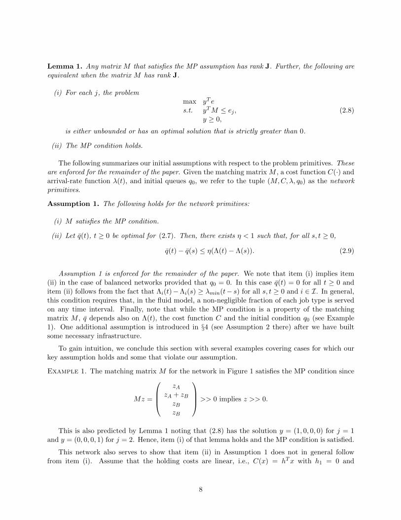
Figure 2: An example with matrix M that has rank strictly less than J.

h2 = h3 = h4 > 0. Suppose that λ = (1, 1, 1, 1). Then, the unique solution to (2.7) is given byz(t) ≡ z = (0, 1) (with an optimal cost of 0). In particular, q1(t) = λ1t so that Assumption 1(ii) isviolated.

Example 2. The M associated with Figure 2

M =

1 0 11 0 10 1 10 1 1

has rank 2 < J = 3 so that, by Lemma 1, the MP condition must be violated.

In a sense, this network is “overly” connected. From a practical point of view, however, onemight think that this can be fixed. Matching B can be restricted to job-types 2 and 3. The resultingnetwork is equivalent in terms of optimality to the one depicted in Figure 3 (every time that B isactivated in the original network one could simultaneously activate A,B,C in the new one). Thatnetwork, however, also violates the MP condition; see below. Thus, a rank strictly less than J doesnot have an “easy” fix.

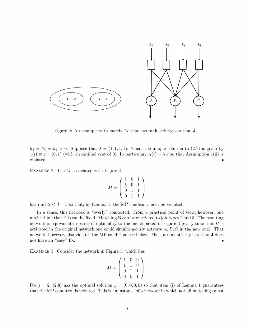
Example 3. Consider the network in Figure 3, which has

M =

1 0 01 1 00 1 10 0 1

.

For j = 2, (2.8) has the optimal solution y = (0, 0, 0, 0) so that item (i) of Lemma 1 guaranteesthat the MP condition is violated. This is an instance of a network in which not all matchings must

9

1 2 3 4 A B

λ2=1 λ1=1 λ3=1

C

λ4=1

Figure 3: An example with no pooling

be used. When λ(t) ≡ λ = (1, 1, 1, 1)T , for example, the unique z that solves (2.7) for all t ≥ 0is z = (zA, zB, zC)T = (1, 0, 1)T , meaning that matching B is not used in the context of the staticmatching problem. For a policy to be optimal in such a setting it would have to be careful not tooveruse matching B but, rather, use it only rarely. This is reminiscent of the notion of non-basicactivities in the context of capacitated queueing networks; see e.g. [19].

A slightly modified network does however satisfy the MP condition; see Example 4.

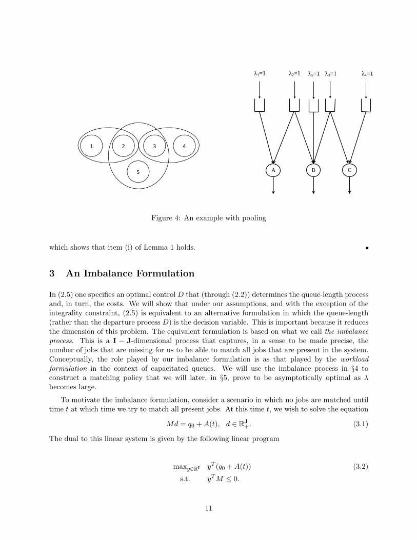
Example 4. Consider the network in Figure 4, which has

M =

1 0 01 1 00 1 10 0 10 1 0

.

Since

Mz =

zA

zA + zBzB + zCzCzB

>> 0 implies z >> 0,

the MP assumption is satisfied. Note that the solution to (2.8) for j = 1, 2, 3 is

j yT

1 (1, 0, 0, 0, 0)2 (0, 0, 0, 0, 1)3 (0, 0, 0, 1, 0)

,

10

1 2 3 4

5

A B

λ2=1 λ1=1 λ3=1

C

λ4=1 λ5=1

Figure 4: An example with pooling

which shows that item (i) of Lemma 1 holds.

3 An Imbalance Formulation

In (2.5) one specifies an optimal control D that (through (2.2)) determines the queue-length processand, in turn, the costs. We will show that under our assumptions, and with the exception of theintegrality constraint, (2.5) is equivalent to an alternative formulation in which the queue-length(rather than the departure process D) is the decision variable. This is important because it reducesthe dimension of this problem. The equivalent formulation is based on what we call the imbalanceprocess. This is a I − J-dimensional process that captures, in a sense to be made precise, thenumber of jobs that are missing for us to be able to match all jobs that are present in the system.Conceptually, the role played by our imbalance formulation is as that played by the workloadformulation in the context of capacitated queues. We will use the imbalance process in §4 toconstruct a matching policy that we will later, in §5, prove to be asymptotically optimal as λbecomes large.

To motivate the imbalance formulation, consider a scenario in which no jobs are matched untiltime t at which time we try to match all present jobs. At this time t, we wish to solve the equation

Md = q0 +A(t), d ∈ RJ+. (3.1)

The dual to this linear system is given by the following linear program

maxy∈RI yT (q0 +A(t)) (3.2)

s.t. yTM ≤ 0.

11

Strong duality implies that (3.1) has a feasible solution if and only if (3.2) has a finite optimalsolution y∗ (any such solution must have here (y∗)T (q0 + A(t)) = 0). This, in turn, holds if andonly if there exists no y such that yTM ≤ 0 and yTA(t) > 0. By complementary slackness wemust have (y∗)T (Md − (q0 + A(t))) = 0. Since d ≥ 0, this implies that (y∗)TM = 0. Thus, afeasible matching d is guaranteed to exist iff there exists an optimal solution y∗ to the dual suchthat (y∗)T (q0 +A(t)) = 0 and (y∗)TM = 0. Any deviation (i.e. if yT (q0 +A(t)) > 0 for some y withyTM ≤ 0) implies that we have a imbalance of jobs: that the arrivals by time t prohibit matchingall the present jobs.

We re-visit this interpretation in Example 5 below. By varying t we can construct a processS = (S(t), t ≥ 0) having S(t) = 0 if there exists d ≥ 0 such that Md = q0 + A(t) and S(t) 6= 0otherwise. More specifically, fix a matrix Y whose rows span

Y = y ∈ RI : yTM = 0, (3.3)

and defineS(t) := Y T (q0 +A(t)) for all t ≥ 0. (3.4)

The process S(t) obtains values in the subspace

M := s ∈ RI−J : Y Tx = s, for some x ≥ 0. (3.5)

The definition of the imbalance process is not unique as there may be multiple choices forthe matrix Y . The choice of Y does not, however, affect our results so we do not make thisdependence explicit in our notation. Regardless of how Y is chosen, its rank is I − J (recall thatrank(M) = J < I). Taking the stochastic-processing-network view (see Remark 1) and recallingthat, under the match pooling condition, there are J basic activities, the fact that the dimensionof the imbalance process is I − J is the perfect analogue of the fact that the dimension of theworkload process in the capacitated setting is I− J under the standard resource pooling condition;see Corollary 6.2 in [7]. Finally, we note that for Y to carry useful information, we must have thatY 6= 0 which may be violated if the MP condition fails to hold, as in Example 3.

The following lemma shows that (S(t), t ≥ 0) plays the desired role in that when S(t) = 0 wecan match all jobs that arrived by time t (assuming they are all present in the network at thattime).

Lemma 2. For each x ≥ 0 such that Y Tx = 0 there exists a unique solution d to the system ofequations Md = x, and this solution is non-negative.

Example 5 (Example 1 Continued). Consider the network in Figure 1 and assume that q0 = 0.Then, y = (1,−1, a, 1− a)T (with any a ∈ (0, 1)) satisfies yTM = yTλ = 0. One possible choice forY is then

Y =

(1 −1 1/2 1/20 0 1 −1

),

so that

S(t) =

(A1(t)−A2(t) + 1

2 (A3(t) +A4(t))A3(t)−A4(t)

).

12

Then, S2(t) = 0 only if A3(t) = A4(t), which is consistent with the fact that all type 3 and 4jobs can be matched only if the exact same number of each type is present. Assuming S2(t) = 0,S1(t) = 0 only if

A2(t) = A1(t) +1

2(A3(t) +A4(t))

= A1(t) +A3(t),

so that there are enough type-2 jobs to match all jobs of types 1, 3, and 4 that are present in thequeues at time t. On the other hand, if S2(t) > 0 when S1(t) = 0 there is a imbalance of type-2jobs, and when S2(t) < 0 there is a imbalance of other job types.

The objective value in the original problem formulation (2.5) is trivially lower bounded by aproblem which is identical with the exception of relaxing the integrality requirements on D: theproblem of minimizing

∫ u0 C (Q(t;D)) dt subject to

Q(t) = q0 +A(t)−MD(t),

D(0) = 0, D(t) is increasing ,∫ ∞0

1Qi (t−) + ∆Ai(t) = 0 for any i ∈ I(j)dDj(t) = 0,

Q(t) ≥ 0, j ∈ J ,

(3.6)

in which the integrality restrictions in (2.5) have been removed. Consider now the following problem:

min

∫ u

0C(q(s))ds,

s.t. Y T q(t) = S(t), for all 0 ≤ t ≤ u,A(t)−A(s) ≥ q(t)− q(s), for all 0 ≤ s ≤ t ≤ u,q(t) ≥ 0, for all 0 ≤ t ≤ u.

(3.7)

An admissible solution to (3.7) is an RCLL process (q(t), t ≥ 0). Under the MP condition the twoformulations are equivalent in a sense made precise in the next theorem.

Theorem 1. If (Q,D) is an admissible solution for (3.6), then, Q is admissible for (3.7) . Con-versely, if Q is an admissible solution for (3.7), then there exists a process D such that (Q,D) isadmissible for (3.6).

Proof: Let (Q,D) be an admissible solution for (3.6). Then, the first equation in (3.6) togetherwith the fact that D is an increasing process guarantee that A(t)−A(s) ≥ Q(t)−Q(s). Also, sinceY TM = 0 by definition, we have that Y TQ(t) = Y T (q0+A(t))−Y TMD(t) = Y T (q0+A(t)) = S(t).Hence, Q is feasible for (3.7). Next, we will show that if Q is a solution to (3.7) then there exists aprocess D such that (Q,D) is a solution to (3.6). This assertion follows, however, easily from thefact that any optimal solution to (3.2) has yTM = 0. Specifically, we construct the process D(t) asfollows: Let x(t) = q0+A(t)−Q(t). Note that since Q is a solution to the formulation (3.7) we have,in particular, that x(t) ≥ 0 and Y Tx(t) = 0. Using Lemma 2 let D(t) be the unique solution to

13

MD(t) = x(t). We claim that the process D(t) constructed this way is, in fact, increasing. Indeed,by construction M(D(t)−D(s)) = x(t)− x(s). Since x(t)− x(s) ≥ 0 (by the second constraint in(3.7)) and since Y Tx(t) = Y Tx(s) = 0, we have by Lemma 2 that D(t)−D(s) must be the unique(non-negative solution) to this system. Thus, D(t) is increasing. Finally, since A(t) is RCLL and sois, by definition q(t), they both have a finite number of discontinuity points on any finite interval.Thus, to show that the third constraints in (3.6) holds, it suffices to show that if (s, t] is an intervalsuch that q(u−) + ∆Ai(u) = 0 u ∈ (s, t] then D(t)−D(s) = 0. This follows, however, noting thatthen Dj(t)−Dj(s)) must be equal to 0 for all j ∈ J (i) (otherwise, we would necessarily have that(M(D(t)−D(s)))i > 0.

Remark 2. It is important that if (Q,D) is a feasible solution to (3.6), then the feasibility ofQ for (3.7) does not require the MP condition. It follows, in particular, that regardless of anyassumptions the optimal value in (3.7) serves as a lower bound for (3.6) and, in turn, for (2.5).

A further lower bound is obtained by removing the constraint A(t) − A(s) ≥ q(t) − q(s) from(3.4).

min

∫ u

0C(q(s))ds,

s.t. Y T q(t) = S(t), for all 0 ≤ t ≤ u,q(t) ≥ 0, for all 0 ≤ t ≤ u,

(3.8)

In our asymptotic optimality proofs we will show that this lower bound is achieved. This willhinge on showing that, in high volume, the constraint A(t) − A(s) ≥ q(t) − q(s) is rarely binding(see Lemma 3 below), so that (3.8) is, in a sense, equivalent to (3.4) which, in turn, by Theorem 1is equivalent to (3.6).

Remark 3 (A “re-shuffle” interpretation). The imbalance formulation (3.8) is similar in spirit tothe workload formulation in [22]. Our multidimensional imbalance process, as their one dimensionalworkload process are invariant to the control that is used and this is the essence of their usefulness.

This formulation has an appealing interpretation within the matching setting related to the dualdemand-supply role discussed in the introduction. When making a matching decision at a giventime t, one is constrained by past matching decisions: jobs that were matched up to time t are notavailable for matching. Ideally, one could ignore past matchings and re-shuffle the matchings madeup to time t. The formulation (3.8) pretends that this is the case.

The problem (3.8) has a trivial solution. Specifically, given a sample path of the imbalanceprocess (S(t), t ≥ 0), an optimal solution for (3.8) is (Q(S(t)), t ≥ 0) where, Q : M→ RI

+ (recall(3.5)) satisfies

Q(s) ∈ argminq≥0

C(q) : Y T q = s. (3.9)

The convexity and monotonicity of C guarantee that (3.9) has an optimal solution (for feasibility, ifs = Y Tx take q = x). We will impose certain requirements onQ. In the next section, we will imposea Lipschitz continuity requirement on Q. Most importantly that it is Lipschitz in its argument (orat least can be selected as such if not unique). We will formally introduce these requirements after

14

1 2 3

A B

λ2=2 λ3=1 λ1=1

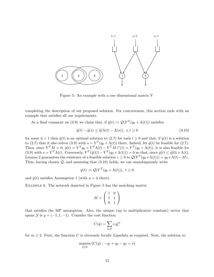
Figure 5: An example with a one dimensional matrix Y

completing the description of our proposed solution. For concreteness, this section ends with anexample that satisfies all our requirements.

As a final comment on (3.9) we claim that, if q(t) := Q(Y T (q0 + Λ(t))) satisfies

q(t)− q(s) ≤ η(Λ(t)− Λ(s)), s, t ≥ 0 (3.10)

for some η < 1 then q(t) is an optimal solution to (2.7) for each t ≥ 0 and that, if q(t) is a solutionto (2.7) that it also solves (3.9) with s = Y T (q0 + Λ(t)) there. Indeed, let q(t) be feasible for (2.7).Then, since Y TM = 0, q(t) = Y T q0 + Y TΛ(t)− Y TMz?(t) = Y T (q0 + Λ(t)), it is also feasible for(3.9) with s = Y TΛ(t). Conversely, Y T (q(t))−Y T (q0 + Λ(t))) = 0 so that, since q(t) ≤ q(0) + Λ(t),Lemma 2 guarantees the existence of a feasible solution z ≥ 0 to Q(Y T (q0+Λ(t))) = q0+Λ(t)−Mz.Thus, having chosen Q, and assuming that (3.10) holds, we can unambiguously write

q(t) := Q(Y T (q0 + Λ(t))), t ≥ 0

and q(t) satisfies Assumption 1 (with η = η there).

Example 6. The network depicted in Figure 5 has the matching matrix

M =

1 01 10 1

that satisfies the MP assumption. Also, the unique (up to multiplicative constant) vector thatspans Y is y = (−1, 1,−1). Consider the cost function

C(q) =∑i∈I

ciqmi

for m ≥ 2. First, the function C is obviously locally Lipschitz as required. Next, the solution to

argminq≥0

C(q) : −q1 + q2 − q3 = s

15

for s ∈M, is

Q1(s) = [−s]+(

(2c1)− 1

m−1

(2c1)− 1

m−1 + (2c3)− 1

m−1

), Q2(s) = [s]+, and Q3(s) = [−s]+

((2c3)

− 1m−1

(2c1)− 1

m−1 + (2c3)− 1

m−1

),

so that Q is, in particular, Lipschitz continuous in s (regardless of m). It is also easily verified that,with c1, c2, c3 > 0 and since λmin(t − s) ≤ Λi(t) − Λi(s) ≤ λmax(t − s) for all s, t and i ∈ I, thereexists η < 1 (not depending on q0) such that q(t) := Q(Y T (q0 + Λ(t))) satisfies Assumption 1(ii).

4 The Proposed Policy

We propose a discrete-review control policy, D?, that solves a static matching problem at reviewtime points

tm = m

(1

λmax

)2/3

for m = 0, 1, 2, . . . , (4.1)

where λmax ≥ λi(t), i ∈ I, t ≥ 0, and does nothing at all other times. We initialize with D?(0) = 0and, at each subsequent review epochs, we perform matchings so as to minimize the instantaneousholding cost; that is, we solve for (dm, qm)

mindm,qm≥0

C(q) (4.2)

subject to:

Y T qm = S(tm), (4.3)

qm = Q(tm−1) +A(tm)−A(tm−1)−Mdm, for each i ∈ I. (4.4)

and then setD?(tm) = D?(tm−1) + d and Q(tm, D?) = qm. (4.5)

The choice for qm is consistent with the pathwise equation for Q in (2.2) and it is straightforward toobserve that the control D? satisfies (2.1)-(2.4) and is thus admissible. If one removes the constraint(4.4), this reduces to the imbalance formulation in (3.8).

Our proposed policy D? does not account for the effect of matchings made in the current periodon future costs that arise due to the constraint (4.4) – it is myopic. We will prove, however, thatwhen the arrival rate is large, the review periods can be carefully chosen so they are (i) sufficientlyshort so that costs do not accumulate between review period, but also (ii) sufficiently long so thatsufficiently many jobs are available for matching at each review period and, in particular, so that(4.4) is (with significant probability) non-binding.

Remark 4 (If Q is not unique). If, for each x ≥ 0, the solution Q(x) in (3.9) is guaranteed to beunique (say, if C(·) is strictly convex), the explicit form of Q is not required in order to use ouralgorithm and generate the optimality results that follow. In the absence of apriori uniqueness wemodify the algorithm slightly and use the explicit expression for Q.

At review epoch tm, if there exists dm ≥ 0 such that (dm,Q(S(tm))) satisfies (4.4) (and,in turn, is optimal for (4.2)-(4.4)) choose this solution, i.e, set Q(tm, D?) = Q(S(tm)) andD?(tm) = D?(tm−1) + dm.

16

In other words, at review epoch tm the algorithm chooses Q(S(tm)) whenever feasible.

Remark 5 (A queue-based implementation). To compute S(t) we must know the cumulativearrivals up to time t, A(t) and the initial queues at time 0, q0. From an implementation point ofview it may be preferable to use real-time queue-length information as in the following alternativealgorithm:

At each review epoch solve for (d, q)

mind,q≥0

C(q) (4.6)

subject to:

Y T qm = Y TQ(tm−), (4.7)

qm = Q(tm−)−Mdm,j , for each i ∈ I. (4.8)

and then proceed as before.

The two algorithms are, of course, closely related. Our original policy is intended (and will beshown to) make the queue length track Q(S(t)). Assume that this goal is achieved up to time tm−1,that is, that Q(tm−1) = Q(S(tm−1)) and, consequently, Y TQ(tm−1) = Y T (q0 + A(tm−1)). SinceQi(tm−) = Qi(tm−1)+Ai(tm−)−Ai(tm−1), we would then have Y TQ(tm−) = Y TA(tm) = S(tm−)and, in words, that the queue length an instant before the review epoch carries the requiredimbalance information.

Before proceding to the asymptotic optimality results, we formalize our requirements on theparametric behavior of solutions to (3.9). This will complete the description of the family ofnetworks that our covered by our analysis.

Lipschitz optimizers in (3.9): The first of our requirements is that Q is (or at least can bechosen so that it is) Lipschitz continuous in s. This is a fairly standard requirement in the contextof asymptotically optimal control; two closely related instances are [23] and [22]; see also [4, 12].Lipschitz selection has been extensively studied in the optimization literature and holds in relativegenerality; see e.g. [5], [13] and also the book [6] where this is discussed.

The second requirement arises from the scope of our results covering both balanced, unbalancedand alternating networks in a single result, whereas typically the focus in the heavy-traffic literatureis on the balanced case (referred to generally as the critically loaded case). Indeed, item (ii) of theassumption is redundant in the case of balanced networks (see below) but holds also beyond.

LetQt(x) := Q(Y T (q0 + Λ(t)) + x)

and recall that q(t) = Q(Y T (q0 + Λ(t)) then Qt below considers fine perturbations around q(t).

Qt(x) = Qt(x)− q(t), and Mt := x ∈ RI−J : Y T (q0 + Λ(t)) + x ∈M

Assumption 2 (properties of Q). The network primitives (M,C, λ, q0) are such that

17

(i) Lipschitz selection: There exists a function Q(·) such that, Q(s) is a minimizer in (3.9)that satisfies (3.10) and, for some κ,

|Q(s1)−Q(s2)| ≤ κ|s1 − s2|, s1, s2 ∈M.

(ii) Directional Lipschitz perturbations: There exists γ > 0 so that

|Qt(x)− Qs(y)| ≤ γ|x− y|+ g(s, t)(|x|+ |y|),

for all x ∈Mt, y ∈Ms and s ≤ t where g(·, ·) is such that, for some δ > 0,

limε→0

supt∈(ε,δ)

g(t− ε, t)4√ε

= 0, and sups,t≥δ

g(s, t) <∞.

If the network is balanced item (ii) of Assumption 2 follows from item (i) since, then, Λ(t) =Mz(t) and, in turn, Y TΛ(t) = Y TMz(t) = 0, so that Assumption 2 (ii) is satisfied with g(·, ·) ≡ 0and γ = κ.

In general, i.e, beyond balanced networks, item (ii) has to be verified for each given combinationof network primitives (general theory can be, again, found in [6]). The reader should thus keep inmind that, in terms of the covered cost functions, our results for the unbalanced case may be morerestrictive than in the balanced case.

Example 6 is an instance in which both parts of our Assumption 2 can be seen to hold (regardlessof whether the network is balanced) or not through direct calculation of Q. Below is anotherexample.

Example 7 (homogeneous costs and arrival functions). A function C(·) : RI+ → R+ is said to behomogeneous if there exists δ such that for all x ∈ R+ and all κ > 0 C(κx) = κδC(x). Assumethat q0 = 0, C(·) is homogeneous and there exists a function c : R+ → R+ such that λi(t) = aic(t).In this case item (ii) of Assumption 2 is implied by item (ii).

To see this, fix s, t > 0 and consider the optimization problem minC(q) : Y T q = Y TΛ(t) + xand minC(q) : Y T q = Y TΛ(s)+y. Then, due to homogeneity these two problems are equivalent,in terms of their optimal-solution sets to the two problems minC(q) : Y T q = Y T + a + x andminC(q) : Y T q = Y Ta+ y. Then, for s, t > 0,

|Qt(x)− Qs(y)| = |tQ(x/t)−Q(y/s)|≤ |sQ(x/t)− sQ(y/s)|+ (t− s)|Q(x/t)|

≤ κ|x− y|+ κ|t− s|t|x|+ κ

(t− s)t|x|,

where κ is the Lipschitz constant from item (i) of Assumption 2. If s = 0 or t = 0 we further haveby item (i) that |f(t, x)− f(s, x)| ≤ κ(|x|+ |y|). Letting γ = κ and

g(s, t) = 1t > 02κ|t− s|/t+ 1t = 0κ

we conclude that|f(t, x)− f(s, y)| ≤ γ|x− y|+ g(s, t)(|x|+ |y|)

and g(·, ·) can be easily verified to satisfy the requirements of the assumption.

18

5 Asymptotic Optimality

In this section we prove that our proposed policy D? is asymptotically optimal in high volume(when λ is large). We consider a sequence of systems, indexed by n. The arrival rate in the nthnetwork is λn(t) := nλ(t) so that λni (t) := nλi(t) is the instantaneous arrival rate of type-i jobsat time t. We assume, without loss of generality, that λmax = 1, so that n is interpreted as themaximal aggregate arrival rate over the time horizon. Per (4.1), we have

tnm = m

(1

n

)2/3

for m = 1, 2, . . . , (5.1)

and bun2/3c review epochs on [0, u]. Our convention is to superscript any process or quantityassociated with the network having arrival rate vector λn by n. Thus, for example, qn0 is the initialqueue-length vector in the nth network. It is standard to construct non-stationary Poisson processfrom unit-rate Poisson processes (Ai, i ∈ I) as follows

Ani (t) = Ai(nΛi(t)), for i ∈ I.

When considering a sequence of networks as above we say that Assumptions 1 and 2 holduniformly in n if they hold for each network in the sequence with constants η (in Assumption 1)and κ, γ in Assumption 2 that are uniform in n.

Given a control Dn, the queue process Qn is constructed exactly as in (2.1)-(2.4) with theexception of A being replaced by An. With some abuse of terminology we henceforth say that asequence Dn is an admissible control if Dn is admissible for each n (i.e., Dn satisfies (2.1)-(2.4)).

From the functional central limit theorem for renewal processes it follows that

An :=An − Λn√

n⇒ A := B Λ, as n→∞, (5.2)

where B is a standard I-dimensional Brownian motion. In turn,

Sn :=Sn − Y T qn0 − Y TΛn√

n⇒ S := Y T A, as n→∞. (5.3)

Recalling the discussion at the end of §3 one expects that, under an optimal policy,

Qn − qn ≈√n,

where qn(t) is the solution to the fluid problem (2.7). If C is Lipschitz continuous then, informally,

C(Qn(t))− C(qn(t)) ≈ Qn − qn ≈√n, (5.4)

and, following standard notions a policy is asymptotically optimal if it induces an error that issmaller than the above “cost of stochasticity”. With general convex cost functions, (5.4) is replacedwith

C(Qn(t))− C(qn(t)) ≈ L(qn(t))(Qn(t)− qn(t)) ≈ L(qn(t))√n, (5.5)

19

where, for κ > 0, L(κ) <∞ is the local Lipschitz constant, i.e,1

L(κ) := supq,q:|q|∨|q|≤κ

|C(q)− C(q)||q − q|

An expansion of the standard notion of asymptotic optimality is then to say that a policy isasymptotically optimal if its distance from the optimum is negligible compared to that cost ofstochasticity.

For the statement of our main theorem, let

Lnu(K) = L(K√n+ ‖qn‖u

).

The next theorem establishes that our proposed control Dn? is asymptotically optimal in high

volume. It applies to both our original policy as well as to the alternative in Remark 5.

Theorem 1. Let u ≥ 0 and suppose that Assumptions 1 and 2 hold uniformly in n. Also, supposethat qn0 = Q(Y T qn0 ). Then,

(i) For any admissible control Dn, and all n,∫ u

0C (Qn(t,Dn)) dt ≥

∫ u

0C(Q(Sn(t)))dt, almost surely. (5.6)

(ii) For the proposed control Dn? and any K > 0,

1√n‖Qn −Q(Sn)‖u ⇒ 0 as n→ 0, (5.7)

and ∫ u

0C(Qn(t,Dn

? ))dt−∫ u

0C(Q(Sn(t)))dt = oP (Lnu(K)

√n), as n→∞. (5.8)

Remark 6 (Initial conditions). As is commonly the case in such asymptotic analysis, it is notnecessary to assume that qn0 = Q(Y T qn0 ). One can extend the result to the case where qn0 −Q(Y T qn0 ) = O(

√n) provided that a relaxed version of (3.10), namely, that there exists t1 > 0 such

that (3.10) holds for s = 0, t = t1/√n and then for all s, t ≥ t1/

√n. In this case the algorithm

is changed to have the first review period be at time tn1 = t1/√n. Our proofs can be adapted to

show that (5.7) turns into suptn1≤t≤u |Qn(t) − Q(Sn(t))|/

√n ⇒ 0 and from there to establishing

asymptotic optimality over [tn1 , u].

It is important that the generality that we allow in terms of initial conditions is more restrictedthan is common in the parallel-sever capacitated case. This is, again, driven by the dual role ofjobs as both supply and demand. As an example consider the simple network in Example 6 withc1 = c2 = c3 = 1. Then, Q1(s) = Q3(s) = [−s]+/2. Assume that λ1 = λ2 = λ3 = 1. Then, it iseasily verified that if qn0 = (3

√n, 0,√n), we are not able to make the queues of type 1 and 3 equal

within a O(1/√n) time. This is driven by “insufficient supply” of type-2 arrivals.

Thus, in contrast to the capacitated case, we can not freely direct capacity to deplete a specificqueue so as to quickly pull it into the so-called invariant manifold. Here, such ability dependsstrongly on arrivals of other job-types.

1Convexity guarantees that the function C is locally Lipschitz.

20

Remark 7 (Some special cases). If C(·) is Lipschitz continuous then the optimality gap is oP (√n)

regardless of whether or not the network is balanced. Note that the optimality holds regardlessof whether or not the lower bound actually converges to a proper limit. Still, in some cases, limitresults can be obtained; see Corollary 1 below.

More generally, the optimality depends on the local Lipschitz constant around the “fluid”.Consider, as in Example 6 separable costs of the form C(q) =

∑i ciq

mi then, Lnu(0) = m(‖qn‖u)m−1.

Thus, if ‖qn‖u = 0, we have that the gap is oP (√n), but if ‖qn‖u ≈ n (as one expects, e.g. in the

unbalanced case), then the optimality gap is oP (nm−1√n).

Remark 8 (General arrival processes). We restricted Theorem 1 to Poisson arrival processes asthis facilitates covering stationary and non-stationary arrivals in one result. This is not, however,strictly necessary. In the case that Λi(t) = λit for all t ≥ 0 and i ∈ I, Theorem 1 is valid withoutchange provided that bounds as in Lemma 7.1 in our appendix hold. This would be the case, forexample, if An1 , ..., A

nI are independent renewal processes with finite 5th moment for the inter-arrival

time (see the proof of Lemma 7.1 and the references therein). In this case, An would also satisfyan FCLT as in (5.2) (with properly defined diffusion coefficients).

Before proceeding the proof of Theorem 1 we state and prove a simple corollary for the balancedlinear-cost case. Below, S is as in (5.3).

Corollary 1 (linear costs and balanced network). Let u ≥ 0 and assume that C(x) = hTx, thenetwork is balanced and that qn0 = Q(Y T qn0 ) for qn0 that satisfies qn0 /

√n→ q0 as n→∞. Then,

(i) For any admissible control Dn, and all n,

lim infn→∞

1√n

∫ u

0hTQn(t,Dn)dt ≥st

∫ u

0hTQ

(Y T q0 + S(t)

)dt.

(ii) For the proposed control Dn? ,

1√n

∫ u

0hTQn(t,Dn

? )dt⇒∫ u

0hTQ

(Y T q0 + S(t)

)dt, as n→∞.

Proof: Part (i) follows directly from part (i) of Theorem 1. Next, as Y TM = 0 we have in thebalanced case that Y TΛn(t) = Y TnΛ(t) = nY TMz?(t) = 0. In turn, Y T (qn0 + An(t)) = Y T (qn0 +

An(t)− Λn(t)) = Y T qn0 +√nSn and Q(Sn(t)) = Q(Y T qn0 +

√nSn(t)). It is easily established that

Q(·) must satisfy for a > 0, that hTQ(x/a) = hTQ(x)/a. In particular, hT (Q(Y T qn0 /√n+ Sn)) =

hT (Q(Y T qn0 +√nSn)/

√n). The Lipschitz continuity of Q, the weak convergence of the imbalance

process in (5.3) and the fact that qn0 /√n→ q0 guarantee that Q(Y T qn0 +

√nSn)⇒ Q(Y T q0 + S).

Equation (5.7) and the Converging Together Theorem imply that

Qn√n⇒ Q(Y T q0 + S) as n→∞.

The continuity of the integral map, and the Continuous Mapping Theorem then show that

1√n

∫ u

0hTQn(t)dt⇒

∫ u

0hTQ(Y T q0 + S(t))dt, as n→∞,

21

as required.

The key to proving Theorem 1 is the following lemma that shows that the queue length is (atleast at review epochs) tracking the value of Q that induces the lower bound.

Lemma 3. Let u ≥ 0 and suppose that the condition of Theorem 1 hold. Then, under the proposedcontrol Dn

? ,

lim infn→∞

PQn (tnm) = Q (Sn(tnm)) for all m = 1, . . . , bun2/3c

= 1, (5.9)

and for any ε > 0 there exists K(ε) such that

lim supn→∞

P‖Qn‖u ∨ ‖Q(Sn)‖u ≥ LnK(ε)

√n≤ ε. (5.10)

Proof of Theorem 1:

From Remark 2, the further lower bound (3.8) and its solution (3.9) it follows that for all n and allt ≥ 0,

C (Qn(t,Dn)) ≥ C(Q(Sn(t)),

which immediately proves (5.6) and we turn to (5.7) and (5.8). In what follows we write Qn(·)instead of Qn(·, Dn

? ).

We claim that (5.8) readily follows from (5.7). Let

An(ε) := ω ∈ Ω : ‖Qn‖u + ‖Q(Sn)|u ≤ LK(ε)

√n.

By Lemma 3, PAn(ε) ≤ 2ε and, on An(ε),

‖C(Qn)− C(Q(Sn))‖u ≤ Lnu(K) ‖Qn −Q(Sn)‖u ,

so that from (5.7) it follows that

P‖C(Qn)− C(Q(Sn))‖u ≥ εL

nK(ε)

≤ 3ε.

Since ε was arbitrary this implies (5.8).

To prove (5.7), note that

‖Qn −Q (Sn)‖u = maxm=0,1,2,...,bu(n)2/3c

suptnm≤t≤t

n+1m

|Qn(t)−Q (Sn(t))| .

Since matches are only made at the review epochs we have that

Qn(t) = Qn(tnm) +An(t)−An(tnm),

22

for t ∈ [tnm, tnm+1). Thus,

1√n‖Qn −Q (Sn)‖u

= maxm=0,1,2,...,bu(n)2/3c

suptnm≤t≤t

n+1m

1√n

∣∣∣∣Qn(tnm)−Q (Sn(tnm)) +An(t)−An(tnm)√

n+Q (Sn(tnm))−Q (Sn(t))

∣∣∣∣≤ max

m=0,1,2,...,bu(n)2/3c

1√n|Qn(tnm)−Q (Sn(tnm))| (5.11)

+ maxm=0,1,2,...,bu(n)2/3c

∣∣∣An(tnm+1)− A(tnm)∣∣∣+ n−1/6λmax (5.12)

+ maxm=0,1,2,...,bu(n)2/3c

suptnm≤t≤tnm+1

1√n|Q (Sn(tnm))−Q (Sn(t))| . (5.13)

The term (5.12) is obtained noting that An(t) − An(s) = Λn(t) − Λn(s) +√n(An(t) − An(s))

and recalling that |Λ(t)−Λ(s)| ≤ λmax(t− s). The term (5.11) weakly converges to 0 by Lemma 3.The weak convergence of An to a continuous limit process in (5.2) implies that the term (5.12)weakly converges to 0. Finally, to prove that (5.13) weakly converges to 0, note that

|Sn(tnm)− Sn(t)| =∣∣Sn(tnm)− Sn(t)− nY T (Λ(tnm+1)− Λ(t))

∣∣+ |Y Tn(Λ(t)− Λ(tnm))|≤

∣∣Sn(tnm+1)− Sn(tnm))− n(Λ(tnm+1)− Λ(tnm))∣∣+ 2yn1/3

≤√n∣∣∣Sn (tnm+1

)− Sn (tnm)

∣∣∣+ 2yn1/3,

for t ∈ (tnm, tnm+1] where y = maxkl |Ykl| and we used the fact that λmax = 1 and tnm+1− tnm = n−2/3.

The Lipschitz continuity of Q then implies

1√n|Q (Sn(tnm))−Q (Sn(t))| ≤ κ

(∣∣∣Sn (tnm+1

)− Sn (tnm)

∣∣∣+ 2n−1/6).

Finally, the right-hand side converges to 0 by the weak convergence of Sn to a continuous limit(5.3), and we may conclude that (5.13) weakly converges to 0 and, in turn, that (5.7) holds.

6 Numerical experiments

We provide some numerical examples for the balanced, unbalanced and non-stationary settings.We use the networks in Figures 1 and 4 and for which the MP condition was verified to hold(see Examples 1 and 4). We refer to these as network I and network II respectively. We considerseparable quadratic cost of the form C(q) =

∑i ciq

2i with the coefficients cT = (2, 1, 5, 7) for network

I and cT = (3, 1, 5, 7, 0) for network II. Separable costs are chosen for implementation simplicity asthey can be specified entirely in terms of the coefficient vector.

We use Poisson arrivals that are stationary or non-stationary depending on the experiment. Wefix the horizon to be [0, 1]. Given a sample path of the arrivals (A(t), 0 ≤ t ≤ 1) we generate two

23

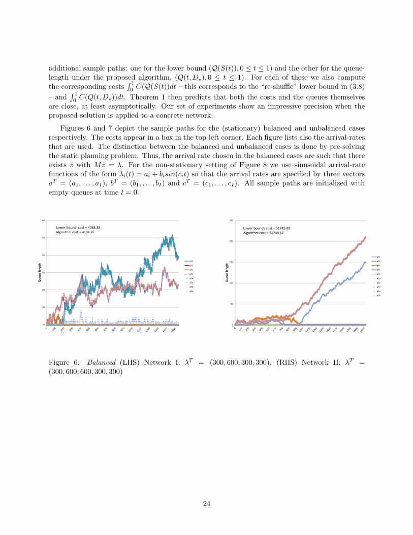
additional sample paths: one for the lower bound (Q(S(t)), 0 ≤ t ≤ 1) and the other for the queue-length under the proposed algorithm, (Q(t,D?), 0 ≤ t ≤ 1). For each of these we also computethe corresponding costs

∫ 10 C(Q(S(t))dt – this corresponds to the “re-shuffle” lower bound in (3.8)

– and∫ 10 C(Q(t,D?))dt. Theorem 1 then predicts that both the costs and the queues themselves

are close, at least asymptotically. Our set of experiments show an impressive precision when theproposed solution is applied to a concrete network.

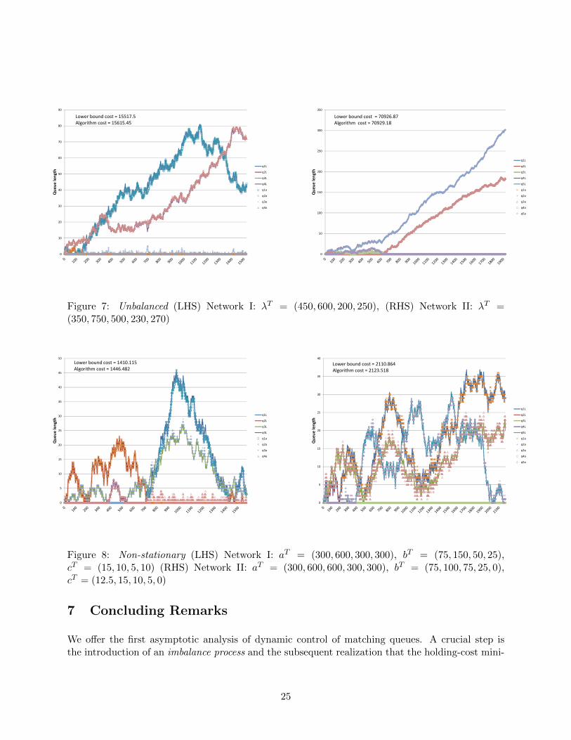
Figures 6 and 7 depict the sample paths for the (stationary) balanced and unbalanced casesrespectively. The costs appear in a box in the top-left corner. Each figure lists also the arrival-ratesthat are used. The distinction between the balanced and unbalanced cases is done by pre-solvingthe static planning problem. Thus, the arrival rate chosen in the balanced cases are such that thereexists z with Mz = λ. For the non-stationary setting of Figure 8 we use sinusoidal arrival-ratefunctions of the form λi(t) = ai + bisin(cit) so that the arrival rates are specified by three vectorsaT = (a1, . . . , aI), b

T = (b1, . . . , bI) and cT = (c1, . . . , cI). All sample paths are initialized withempty queues at time t = 0.

0

10

20

30

40

50

60

Que

ue length

q1L

q2L

q3L

q4L

q1a

q2a

q3a

q4a

Lower bound cost = 4063.38Algorithm cost = 4194.87

0

50

100

150

200

250

Que

ue length

q1L

q2L

q3L

q4L

q5L

q1a

q2a

q3a

q4a

q5a

Lower bounds cost = 51745.89 Algorithm cost = 51749.67

Figure 6: Balanced (LHS) Network I: λT = (300, 600, 300, 300), (RHS) Network II: λT =(300, 600, 600, 300, 300)

24

0

10

20

30

40

50

60

70

80

90

Que

ue length

q1L

q2L

q3L

q4L

q1a

q2a

q3a

q4a

Lower bound cost = 15517.5Algorithm cost = 15615.45

0

50

100

150

200

250

300

350

Que

ue length

q1L

q2L

q3L

q4L

q5L

q1a

q2a

q3a

q4a

q5a

Lower bound cost = 70926.87Algorithm cost = 70929.18

Figure 7: Unbalanced (LHS) Network I: λT = (450, 600, 200, 250), (RHS) Network II: λT =(350, 750, 500, 230, 270)

0

5

10

15

20

25

30

35

40

45

50

Que

ue length

q1L

q2L

q3L

q4L

q1a

q2a

q3a

q4a

Lower bound cost = 1410.115Algorithm cost = 1446.482

0

5

10

15

20

25

30

35

40

Que

ue length

q1L

q2L

q3L

q4L

q5L

q1a

q2a

q3a

q4a

q5a

Lower bound cost = 2110.864Algorithm cost = 2123.518

Figure 8: Non-stationary (LHS) Network I: aT = (300, 600, 300, 300), bT = (75, 150, 50, 25),cT = (15, 10, 5, 10) (RHS) Network II: aT = (300, 600, 600, 300, 300), bT = (75, 100, 75, 25, 0),cT = (12.5, 15, 10, 5, 0)

7 Concluding Remarks

We offer the first asymptotic analysis of dynamic control of matching queues. A crucial step isthe introduction of an imbalance process and the subsequent realization that the holding-cost mini-

25

mization problem can be solved asymptotically by considering an equivalent imbalance formulation.Our use of the equivalent imbalance formulation is conceptually similar to that of the equivalentworkload formulation in the context of parallel-server queueing networks.

The execution, however, differs substantially. In the matching setting arrivals play (also) therole of capacity. From a control perspective, the implication is an inability to instantaneously“re-balance” the queues by focusing processing resources on a subset of the queues. Then, it isa priori unclear what the conceptual equivalents of ”workload” and ”resource pooling” are in thematching setting. Even though the matching setting shares with the parallel-server capacitatedsetting the phenomena of dimensionality reduction, the equivalent imbalance formulation is notone dimensional. Furthermore, under a match pooling condition, we show how to exploit theimbalance process to construct a sample path lower bound and a discrete-review matching policythat asymptotically attains this lower bound as the arrival rates become large, for both stationaryand time-varying arrivals. This stands in contrast with the parallel-server capacitated setting,where non-stationary arrivals are more difficult to handle.

From a queueing-optimal-control perspective, dynamic matching is closely related to so-calledfork-join queues in which a join station is, in fact, a matching queue: the server can process jobsonly when there are available jobs in all the queues served at that station. We believe that theidea of considering imbalances rather than workloads could contribute to the understanding of suchnetworks that, so far, have received limited attention compared to other types of queueing networks.

Another interesting direction for future research is the application of the ideas in this modelto the centralized control problem for kidney exchanges. In that setting, a job consists of a pair– consisting of a “needy” person and a “donor”. The donor is not necessarily compatible withthe needy and so may not be able to directly donate a kidney to his needy partner. A givenpair, however, may be matched with another pair such that the needy person of the first pair iscompatible with the donor of the second. This can also be part of larger (i.e., including more thantwo pairs) chains. [2] and [1] both argue that allowing for long chains is important. However, itcan be seen from [29] that allowing for long chains is hard. We are hopeful that the constructionof an equivalent imbalance formulation in this setting may be helpful, because it allowed for us tomove beyond analyzing bipartite matching structures.

Appendix

Proof of Lemma 1:

For the first part of the lemma suppose towards contradiction that rank(M) < J. Then, thereexists z 6= 0 such that Mz = 0. Fix any z ≥ 0 such that λ := Mz 0 (this can be done since, foreach i there exists j with Mij = 1). Then, for any constant K

M (z −Kz) = λ.

By the definition of MP, and since λ 0 we must have that z −Kz ≥ 0. However, since z 6= 0we can now K with |K| large enough so that z−Kz < 0. This is a contradiction. In turn, we must

26

have that rank(M) = J.

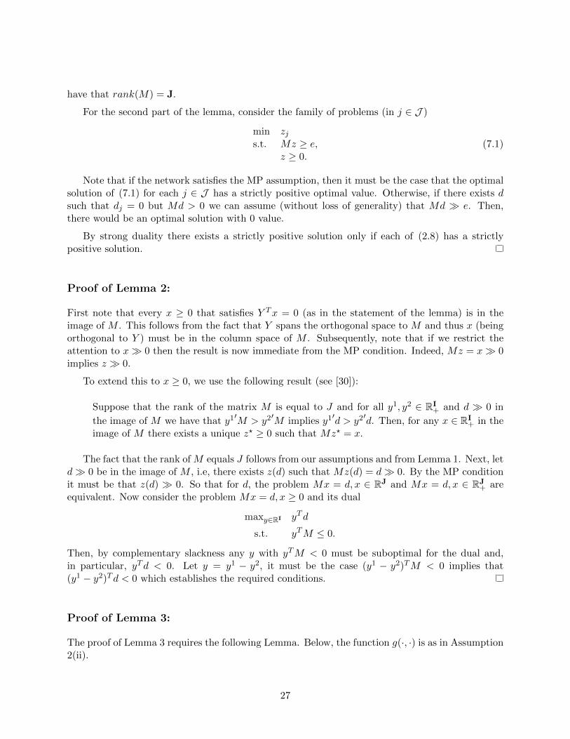
For the second part of the lemma, consider the family of problems (in j ∈ J )

min zjs.t. Mz ≥ e,

z ≥ 0.(7.1)

Note that if the network satisfies the MP assumption, then it must be the case that the optimalsolution of (7.1) for each j ∈ J has a strictly positive optimal value. Otherwise, if there exists dsuch that dj = 0 but Md > 0 we can assume (without loss of generality) that Md e. Then,there would be an optimal solution with 0 value.

By strong duality there exists a strictly positive solution only if each of (2.8) has a strictlypositive solution.

Proof of Lemma 2:

First note that every x ≥ 0 that satisfies Y Tx = 0 (as in the statement of the lemma) is in theimage of M . This follows from the fact that Y spans the orthogonal space to M and thus x (beingorthogonal to Y ) must be in the column space of M . Subsequently, note that if we restrict theattention to x 0 then the result is now immediate from the MP condition. Indeed, Mz = x 0implies z 0.

To extend this to x ≥ 0, we use the following result (see [30]):

Suppose that the rank of the matrix M is equal to J and for all y1, y2 ∈ RI+ and d 0 in

the image of M we have that y1′M > y2

′M implies y1

′d > y2

′d. Then, for any x ∈ RI

+ in theimage of M there exists a unique z? ≥ 0 such that Mz? = x.

The fact that the rank of M equals J follows from our assumptions and from Lemma 1. Next, letd 0 be in the image of M , i.e, there exists z(d) such that Mz(d) = d 0. By the MP conditionit must be that z(d) 0. So that for d, the problem Mx = d, x ∈ RJ and Mx = d, x ∈ RJ

+ areequivalent. Now consider the problem Mx = d, x ≥ 0 and its dual

maxy∈RI yTd

s.t. yTM ≤ 0.

Then, by complementary slackness any y with yTM < 0 must be suboptimal for the dual and,in particular, yTd < 0. Let y = y1 − y2, it must be the case (y1 − y2)TM < 0 implies that(y1 − y2)Td < 0 which establishes the required conditions.

Proof of Lemma 3:

The proof of Lemma 3 requires the following Lemma. Below, the function g(·, ·) is as in Assumption2(ii).

27

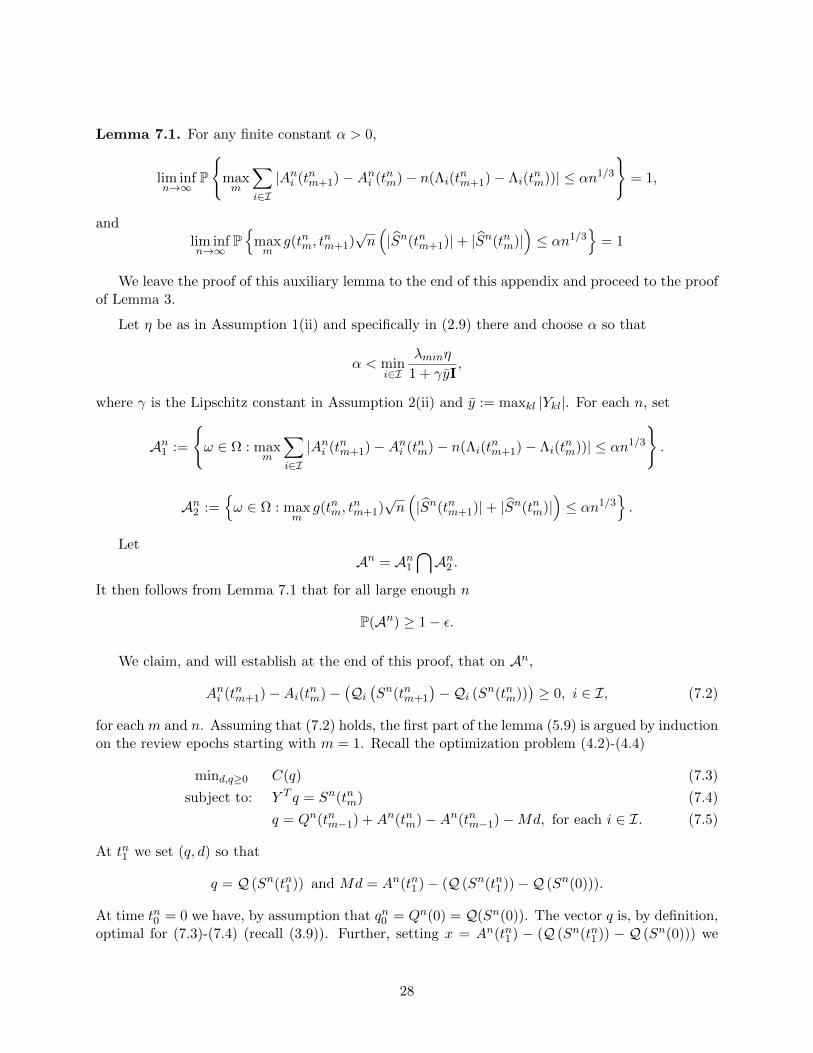
Lemma 7.1. For any finite constant α > 0,

lim infn→∞

P

maxm

∑i∈I|Ani (tnm+1)−Ani (tnm)− n(Λi(t

nm+1)− Λi(t

nm))| ≤ αn1/3

= 1,

andlim infn→∞

P

maxm

g(tnm, tnm+1)

√n(|Sn(tnm+1)|+ |Sn(tnm)|

)≤ αn1/3

= 1

We leave the proof of this auxiliary lemma to the end of this appendix and proceed to the proofof Lemma 3.

Let η be as in Assumption 1(ii) and specifically in (2.9) there and choose α so that

α < mini∈I

λminη

1 + γyI,

where γ is the Lipschitz constant in Assumption 2(ii) and y := maxkl |Ykl|. For each n, set

An1 :=

ω ∈ Ω : max

m

∑i∈I|Ani (tnm+1)−Ani (tnm)− n(Λi(t

nm+1)− Λi(t

nm))| ≤ αn1/3

.

An2 :=ω ∈ Ω : max

mg(tnm, t

nm+1)

√n(|Sn(tnm+1)|+ |Sn(tnm)|

)≤ αn1/3

.

LetAn = An1

⋂An2 .

It then follows from Lemma 7.1 that for all large enough n

P(An) ≥ 1− ε.

We claim, and will establish at the end of this proof, that on An,

Ani (tnm+1)−Ai(tnm)−(Qi(Sn(tnm+1

)−Qi (Sn(tnm))

)≥ 0, i ∈ I, (7.2)

for each m and n. Assuming that (7.2) holds, the first part of the lemma (5.9) is argued by inductionon the review epochs starting with m = 1. Recall the optimization problem (4.2)-(4.4)

mind,q≥0 C(q) (7.3)

subject to: Y T q = Sn(tnm) (7.4)

q = Qn(tnm−1) +An(tnm)−An(tnm−1)−Md, for each i ∈ I. (7.5)

At tn1 we set (q, d) so that

q = Q (Sn(tn1 )) and Md = An(tn1 )− (Q (Sn(tn1 ))−Q (Sn(0))).

At time tn0 = 0 we have, by assumption that qn0 = Qn(0) = Q(Sn(0)). The vector q is, by definition,optimal for (7.3)-(7.4) (recall (3.9)). Further, setting x = An(tn1 ) − (Q (Sn(tn1 )) − Q (Sn(0))) we

28

have by (7.2) that x ≥ 0 and Y Tx = 0 so that by Lemma 2, d as above exists. Thus, (q, d) isfeasible and optimal for (7.3)-(7.5).

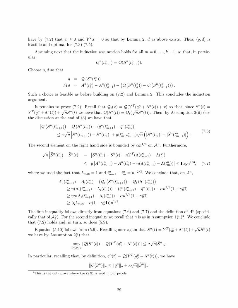
Assuming next that the induction assumption holds for all m = 0, . . . , k− 1, so that, in partic-ular,

Qn(tnk−1) = Q(Sn(tnk−1)).

Choose q, d so that

q = Q (Sn(tnk))

Md = An(tnk)−An(tnk−1)−(Q (Sn(tnk))−Q

(Sn(tnk−1)

)).

Such a choice is feasible as before building on (7.2) and Lemma 2. This concludes the inductionargument.

It remains to prove (7.2). Recall that Qt(x) = Q(Y T (qn0 + Λn(t)) + x) so that, since Sn(t) =

Y T (qn0 + Λn(t)) +√nSn(t) we have that Q(Sn(t)) = Qt(

√nSn(t)). Then, by Assumption 2(ii) (see

the discussion at the end of §3) we have that∣∣Q (Sn(tnm+1))−Q (Sn(tnm))− (qn(tnm+1)− qn(tnm))

∣∣≤ γ√n∣∣∣Sn(tnm+1))− Sn(tnm)

∣∣∣+ g(tnm, tnm+1)

√n(|Sn(tnm)|+ |Sn(tnm+1)|

).

(7.6)

The second element on the right hand side is bounded by αn1/3 on An. Furthermore,

√n∣∣∣Sn(tnm)− Sn(t)

∣∣∣ =∣∣Sn(tnm)− Sn(t)− nY T (Λ(tnm+1)− Λ(t))

∣∣≤ y

∣∣An(tnm+1)−An(tnm)− n(Λ(tnm+1)− Λ(tnm))∣∣ ≤ Iαyn1/3, (7.7)

where we used the fact that λmax = 1 and tnm+1 − tnm = n−2/3. We conclude that, on An,

Ani (tnm+1)−Ai(tnm)−(Qi(Sn(tnm+1)

)−Qi (Sn(tnm))

)≥ n(Λi(t

nm+1)− Λi(t

nm)))− (qn(tnm+1)− qn(tnm))− αn1/3(1 + γyI)

≥ ηn(Λi(tnm+1)− Λi(t

nm)))− αn1/3(1 + γyI)

≥ (ηλmin − α(1 + γyI))n1/3.

The first inequality follows directly from equations (7.6) and (7.7) and the definition of An (specifi-cally that of An2 ). For the second inequality we recall that η is as in Assumption 1(ii)2. We concludethat (7.2) holds and, in turn, so does (5.9).

Equation (5.10) follows from (5.9). Recalling once again that Sn(t) = Y T (qn0 +Λn(t))+√nSn(t)

we have by Assumption 2(i) that

sup0≤t≤u

|Q(Sn(t))−Q(Y T (qn0 + Λn(t)))| ≤ κ√n|Sn|u.

In particular, recalling that, by definition, qn(t) = Q(Y T (qn0 + Λn(t))), we have

‖Q(Sn)‖u ≤ ‖qn‖u + κ√n‖Sn‖u.

2This is the only place where the (2.9) is used in our proofs.

29

We next consider Qn. Recall that (5.7) in Theorem 1 does not use (5.10) so we may use it here.Specifically, by (5.7), we have

‖Q(Sn)‖u ∨ ‖Qn‖u ≤ ‖Q(Sn)‖u ∨ (‖Q(Sn)‖u +√nεn) (7.8)

with εn → 0 in probability as n→∞. Since Sn converges weakly (see (5.3)), it is also stochasticallybounded and given ε > 0 we may choose K(ε) such that

P‖Q(Sn)‖u ∨ ‖Qn‖u > K(ε)√n+ ‖qn‖u ≤ Pκ‖Sn‖u > K(ε)/2 ≤ ε, (7.9)

as required.

Proof of Lemma 7.1: The first part follows from [3] (see the explanation in the proof of Lemma4.1 in [23]). We do not repeat the proof. For the second part note by strong approximationtheorems we have that, on [0, u],

√nAn(t) = Bi(nΛ(t))+O(n1/4 log n). More precisely, there exists

a Brownian motion Bi and a constant c such that

lim supn→∞

P sup0≤t≤λmaxu

√n|Ani (t)−Bi(t))| > cn1/4(log n)3/4 = 0;

see e.g. [20, Theorem 2.1]. For simplicity of notation we let B(t) be B(Λ(t)). For all sufficientlylarge n, cn1/4 log n < αn1/3 so that it suffices to focus on the Brownian term and, specifically, provethat

lim infn→∞

P

maxm

g(tnm, tnm+1)

√ny(|B(tnm+1)|+ |B(tnm)|

)> αn1/3

= 0.

Let mn = dn1/6e and let xnm := g(tnm, tnm+1)

√ny(|B(tnm+1)|+ |B(tnm)|

). Then,

P

maxm≤bun2/3c

xnm > αn1/3≤ P

maxm≤mn

xnm > αn1/3

+ P

maxmn<m<bun2/3c

xnm > αn1/3, (7.10)

and we will argue that each of the elements on the right-hand side converges to 0 as n→∞ startingwith the latter. Specifically, note that

P

maxm>mn

xnm > αn1/3≤ P

maxm>mn

g(tnm, tnm+1)

√n2y‖B‖u > αn1/3

= P

maxm>mn

g(tnm, tnm+1)n

1/62y‖B‖u > α

→ 0

and the convergence follows from basic properties of Brownian motion and the assumption on thefunction g(s, t). Indeed, by Assumption 2(ii), given θ, there exists ε(θ) such that g(t−ε, t) ≤ 4

√ε for

all ε ≤ ε(θ). In turn, we can choose θn → 0 and ε(θn)→ 0 such that θn > n−2/3 for all sufficientlylarge n and so that g(t − n−2/3, t) ≤ θnn−1/6 and, in turn, that n1/6g(tnm, t

nm+1) → 0 as n → ∞.

It then follows from basic properties of Brownian motion (see e.g. [24, Excercise II.1.23]) thatP‖B‖u > 1/θn → 0, as n→∞.

We turn to treat the first element on the right-hand side of (7.10). Observe that for m ≤ n1/6,tnm ≤ 2/

√n. In turn, |B(tnm)| + |B(tnm+1)| ≤ 2‖B‖2/√n. So that, since g = sups,t≤u g(s, t) < ∞ by

Assumption 2(ii) we have that

P

maxm≤mn

g(tnm, tnm+1)

√ny(|B(ntnm+1)|+ |B(ntnm)|

)> αn1/3

≤ P

2gy√n‖B‖2/√n > αn1/3

→ 0,

30

where the convergence follows again from basic properties of Brownian motion.

Acknowledgements: We thank Rakesh Vohra for suggestions that motivated this work. Weare extremely grateful to Kibaek Kim for writing the simulation and optimization code for ournumerical experiments.

References

[1] I. Ashlagi, D. Gamarnik, M. A. Rees, and A. E. Roth. The need for (long) chains in kid-ney exchange, 2011. National Bureau of Economic Research Market Design Working GroupMeeting.

[2] I. Ashlagi and A.E. Roth. New challenges in multi-hospital kidney exchange. AmericanEconomic Review, Papers and Proceedings, 2012. forthcoming.

[3] B. Ata and S. Kumar. Heavy traffic analysis of open processing networks with completeresource pooling: Asymptotic optimality of discrete review policies. Annals of Applied Proba-bility, 2005.

[4] R. Atar. Scheduling control for queueing systems with many servers: Asymptotic optimalityin heavy traffic. The Annals of Applied Probability, 15(4):2606–2650, 2005.

[5] J.P. Aubin. Lipschitz behavior of solutions to convex minimization problems. Mathematics ofOperations Research, pages 87–111, 1984.

[6] J.F. Bonnans and A. Shapiro. Perturbation analysis of optimization problems. Springer Verlag,2000.

[7] M. Bramson and RJ Williams. Two workload properties for brownian networks. QueueingSystems, 45(3):191–221, 2003.

[8] A. Busic, V. Gupta, and J. Mairesse. Stability of the bipartite matching model, 2010. Workingpaper, available through ArXiv.

[9] R. Caldentey, E. H. Kaplan, and G. Weiss. FCFS infinite bipartite matching of servers andcustomers. Adv. Appl. Probab, 41(3):695–730, 2009.

[10] J. G. Dai and W. Lin. Maximum pressure policies in stochastic processing networks. OperationsResearch, 53(2):197–218, 2005.

[11] J. G. Dai and W. Lin. Asymptotic optimality of maximum pressure policies in stochasticprocessing networks. The Annals of Applied Probability, 18(6):2239–2299, 2008.

[12] I. Gurvich and W. Whitt. Scheduling flexible servers with convex delay costs in many-serverservice systems. Manufacturing & Service Operations Management, 11(2):237–253, 2009.

31

[13] W.W. Hager. Lipschitz continuity for constrained processes. SIAM Journal on Control andOptimization, 17:321, 1979.

[14] J. M. Harrison. The BIGSTEP approach to flow management in stochastic processing networks.In F. Kelly, S. Zachary, and I. Ziedins, editors, Stochastic Networks: Theory and Applications,pages 57–90. Oxford University Press, 1996.

[15] J. M. Harrison. Brownian models of open processing networks: Canonical representation ofworkload. Ann. Appl. Prob., 10:75–103, 2000.

[16] J. M. Harrison. A broader view of Brownian networks. Ann. Appl. Probab., 13:1119–1150,2003.

[17] J. M. Harrison. Correction: Brownian models of open processing networks: Canonical repre-sentation of workload. Ann. Appl. Prob., 16(3):1703–1732, 2006.

[18] J. M. Harrison and M. J. Lopez. Heavy traffic resource pooling in parallel-server systems.Queueing Systems, 33:339–368, 1999.

[19] J.M. Harrison and M.J. Lopez. Heavy traffic resource pooling in parallel-server systems.Queueing systems, 33(4):339–368, 1999.

[20] L. Horvath. Strong approximation of renewal processes. Stochastic processes and their appli-cations, 18(1):127–138, 1984.

[21] L. Jiang and J. Walrand. Stable and utility-maximizing scheduling for stochastic processingnetworks. In Forty-Seventh Allerton Conferece Proceedings, Sept. 30 - Oct. 2 2009.

[22] A. Mandelbaum and S. Stolyar. Scheduling flexible servers with convex delay costs: Heavy-traffic optimality of the generalized cµ-rule. Operations Research, 52:836–855, 2004.

[23] Erica L. Plambeck and Amy R. Ward. Optimal control of a high-volume assemble-to-ordersystem. Mathematics of Operations Research, 31(3):453–477, 2006.

[24] D. Revuz and M. Yor. Continuous martingales and Brownian motion, volume 293. SpringerVerlag, 1999.

[25] J. S. Song and P. Zipkin. Supply chain operations: Assemble-to-order and configure-to-ordersystems. In Handbooks in Operations Research and Management Science, volume XXX, pages561–593, 2003.

[26] A. L. Stoylar. Maxweight scheduling in a generalized switch: State space collapse and workloadminimization in heavy traffic. The Annals of Applied Probability, 14(1):1–53, 2004.

[27] L. Tassiulas and A. Ephremides. Stability properties of constrained queueing systems andscheduling policies for maximum throughput in multihop radio networks. IEEE Trans. Au-tomat. Control, 37:1936–1948, 1992.

[28] L. Tassiulas and A. Ephremides. Dynamic server allocation to parallel queues with randomlyvarying connectivity. IEEE Trans. Inform. Theory, 39:466–478, 1993.

32

[29] M. Unver. Dynamic kidney exchange. Review of Economic Studies, 77(1):372–414, 2010.

[30] A. Villar. The generalized linear production model: solvability, nonsubstitution and produc-tivity measurement. The BE Journal of Theoretical Economics, 3(1):1, 2003.

[31] R. J. Williams. On dynamic scheduling of a parallel server system with complete resourcepooling. In D. R. McDonald and S. R. E. Turner, editors, Analysis of Communication Net-works: Call Centres, Traffic and Performance, volume 28 of Fields Institute Communications.American Mathematical Society, 2000.

33