Embed Size (px)
Citation preview
On the Distribution and Dynamics of Health
Care Costs
Eric French
Federal Reserve Bank of Chicago
230 South LaSalle Street
Chicago, IL 60604-1413
John Bailey Jones∗
Department of Economics, BA-110
University at Albany
State University of New York
Albany, New York 12222
November 4, 2003
Abstract
Using data from the Health and Retirement Survey and the Assets and Health Dy-
namics of the Oldest Old survey, we estimate the stochastic process that determines both
the distribution and dynamics of health care costs. We find that the data generating
process for log health costs is well represented as the sum of a white noise process and
a highly persistent AR(1) process. We also find that the innovations to this process can
be modelled with a normal distribution that has been adjusted to capture the risk of
catastrophic health care costs. Simulating this model, we find that in any given year
0.1% of households receive a health cost shock with a present value of at least $125,000.
∗We thank John Rust for encouraging us to write this paper. We also thank Meredith Crowley, HampLankford, Jonathan Skinner, Dan Sullivan, and seminar participants at the Conference on Social Insuranceand Pensions Research in Aarhus, Denmark, the Econometric Society, the Chicago Fed, and the NBERsummer institute for useful comments. Three anonymous referees and especially editor Bent Jesper Christensenprovided extremely detailed and helpful comments. Diwakar Choubey, Kate Godwin, Ken Housinger, KirtiKamboj, Tina Lam, and Santadarshan Sadhu provided excellent research assistance. The research reportedherein was funded in part by a grant from the U.S. Social Security Administration (SSA) to the Center forRetirement Research at Boston College. The views of the authors do not necessarily reflect those of the FederalReserve System or the SSA.
1

1 Introduction
Despite nearly universal health insurance coverage, America’s elderly still face the risk of
catastrophic health care expenses (Crystal et al., 2000). In response to this problem, there
have been many proposals to expand the coverage provided by Medicare, America’s public
health insurance system for the elderly.1 Hoping to clarify the debate on Medicare reform,
numerous researchers have documented the health cost risk that older Americans face in any
given year. However, this literature typically does not consider the distribution of health
care expenditures over extended periods.2 Using panel data from the Health and Retirement
Survey (HRS) and the Assets and Health Dynamics of the Oldest Old (AHEAD) survey,
we analyze both the distribution and dynamics of health care expenditures. This allows us
to consider not only the risk of catastrophic expenses in a single year, but also the risk of
moderate but persistent expenses that accumulate into a catastrophic lifetime cost.
We begin our analysis by examining the time series properties of health costs. To our
knowledge, the only time series model of the health cost process from a nationally representa-
tive sample is that of Feenberg and Skinner (1994).3 We re-evaluate Feenberg and Skinner’s
results, using data that are 20 years more recent and a sample that is, in several ways, more
comprehensive. We find that the autocorrelation structure of log health costs is reasonably
well represented by the sum of an AR(1) component and a white noise component. The
AR(1) component is quite persistent, so that health cost shocks can have a large impact on
lifetime wealth. Because this sum can be rewritten as an ARMA(1,1) process, our results
comport with Feenberg and Skinner’s findings.
We then consider the cross-sectional distribution of health costs. Feenberg and Skinner
assume that the cross section follows a lognormal distribution. Rust and Phelan (1997) argue
that the right tail of the health cost distribution is better represented by a Pareto distribution.
When these two distributions have the same variance, the Pareto distribution has a fatter
1For example, Medicare does not pay for drugs or nursing home or hospital stays over 150 days.2The persistence of health care costs has been considered more carefully in the literature investigating
whether the elderly maintain high asset levels (Hubbard et al., 1994; Palumbo, 1999; Dynan et al., 2002)or delay retirement (Rust and Phelan, 1997; Blau and Gilleskie, 2001; French and Jones, 2003) in order to“buffer” themselves against uncertain medical expenses.
3We are aware of two other papers that consider the persistence of health costs. Eichner et al. (1998)non-parametrically model health costs of insured individuals from a single firm. Palumbo (1999) models thepersistence of health costs coming from persistence in health status. Both models are useful contributions,but neither can be used to infer the lifetime incidence of health costs for a representative sample.
2
right tail than the lognormal, implying a higher probability of catastrophic health care costs.
Neither set of authors, however, formally tests between the two distributions.
Using the likelihood ratio test developed by Vuong (1989), we conclude that the (trun-
cated) lognormal and Pareto specifications fit the top decile of the health cost distribution
equally well. In contrast, we find that the lognormal does a much better job of fitting the
entire distribution. The lognormal distribution that best fits the overall cross section (in
log-likelihood terms), however, understates the right tail of the distribution, and thus under-
states the risk of a catastrophic health cost shock. To address this problem, we construct the
“fitted” lognormal distribution, which matches exactly the mean and the 99.5th percentile
of the empirical distribution. This model fits the upper, catastrophic, portion of the health
cost distribution much more closely than the standard lognormal model.
To complete our model of the stochastic process for health care costs, we need the distri-
bution of log health cost innovations. Because the sum of an AR(1) and a white noise process
is not a Markov process, we cannot use our time series model to back out an empirical distri-
bution of log health cost innovations. We can, however, infer the innovation distribution from
the cross-sectional distribution: if the innovations in our time series model follow a normal
distribution, the cross-sectional distribution will follow a normal distribution as well. This
allows us to estimate a complete model, by finding the Gaussian time series model that best
matches the autocorrelation structure of log health costs and the mean and 99.5th percentile
of health costs themselves. Using this model to simulate health cost histories, we find that
in any given year 0.1% of households receive a health cost shock that exceeds $125,000 in
present value. This is considerably more risk than is generated by the models of Feenberg
and Skinner (1994) and Hubbard et al. (1994).
The rest of the paper is organized as follows. In Section 2, we describe the health cost
data contained in the HRS and AHEAD surveys. In Section 3, we examine the correlation of
health care costs across time, and in Section 4, we examine the cross-sectional distribution. In
Section 5, we estimate lifetime health cost risk by simulating our preferred health cost model.
We conclude in Section 6. Additional results and discussion, including technical appendices,
can be found in a companion paper that is available on line.4
4The companion paper can be found at http://www.chicagofed.org/economists/EricFrench.cfm/ andhttp://www.albany.edu/~jbjones/papers.htm.
3

2 Data
We use data from the HRS and AHEAD surveys. Because the HRS and the AHEAD
data are collected by the same researchers at the University of Michigan, the two data sets
have similar sample designs, allowing us to merge them together. The HRS is a sample of
non-institutionalized individuals, aged 51-61 in 1992, and their spouses. A total of 12,652
individuals in 7,608 households were interviewed in 1992. These individuals were interviewed
again in 1994, 1996, 1998, and 2000. The AHEAD is a sample of non-institutionalized
individuals, aged 70 or older in 1993. A total of 8,222 individuals in 6,047 households were
interviewed for the AHEAD survey in 1993. These individuals were interviewed again in
1995, 1998, and 2000. Because the health insurance and health cost data are incomplete in
wave 1 of both datasets, we use waves 2 through 5 in the analyses below.
Table 1 presents means and standard deviations of variables that measure health care
costs, health insurance coverage, health care utilization, and demographic features. All of
these variables are measured at the household level. To annualize the data, we divide the
health cost and health care utilization measures by the number of years since the individual
was last interviewed, which is, on average, two.
Virtually all Americans aged 65 and older are eligible for insurance through the govern-
ment’s Medicare program. We therefore split the sample between those younger than 65 and
those older than 65. Note that after age 65 nearly everyone has some form of insurance,
although the fraction of individuals with employer-provided coverage falls, as many workers
lose their employer-provided coverage when they leave their job. The other major form of
publicly-provided health insurance is Medicaid, which is available to individuals with low
income and very few assets. Those who report not having any insurance are assigned to the
“none” category.
The variable of interest in this study is the total amount of health care costs paid by
the household. Health care costs are the sum of what the household spends on insurance
premia, drug costs, and costs for hospital, nursing home care, doctor visits, dental visits, and
outpatient care.5 For our sample, mean household health care costs for those younger than
65 are $2,365 and mean costs for those aged 65 and older are $2,805. This compares to the
US average of $2,832 per capita for households headed by a non-institutionalized individual
5See French and Kamboj (2003) for a more detailed description of the data.
4

Age < 65 Age ≥ 65Variable Mean Std. Dev. Mean Std. Dev.
Annual health care costs (in 1998 dollars) 2, 365 (4, 271) 2, 805 (6, 072)Male head of household 0.64 (0.48) 0.51 (0.50)Married 0.48 (0.50) 0.37 (0.48)Age 58.5 (3.6) 76.9 (8.1)No insurance (none) 0.15 (0.36) 0.01 (0.11)Employer-provided insurance 0.61 (0.49) 0.28 (0.45)Privately-purchased insurance 0.10 (0.31) 0.25 (0.43)Medicaid 0.09 (0.28) 0.15 (0.36)Medicare 0.05 (0.22) 0.31 (0.46)Income (in 000s of 1998 dollars) 49.8 (100.5) 29.6 (45.5)Assets (in 000s of 1998 dollars) 249.8 (756.9) 298.0 (1, 113)Annual doctor visits 6.2 (10.3) 7.2 (9.9)Annual nursing home nights 0.7 (14.9) 8.0 (48.6)Annual hospital nights 1.2 (4.9) 2.1 (6.8)
N = 15, 990 N = 18, 903
Table 1: Sample Statistics
aged 65 or older (Federal Interagency Forum on Aging-Related Statistics, 2000). Note that
even though most individuals are insured, there is a great deal of variation in health care
costs. The standard deviation of health care costs is $4,271 for those younger than 65 and
$6,072 for those older than 65. Although this figure is large, it is not surprising, because most
health insurance plans have deductible and/or co-pay provisions. Moreover, many insurance
plans (such as Medicare) do not cover prescription drugs.
One important reason why average health care costs in the HRS/AHEAD data are below
the national average is that individuals in the HRS/AHEAD spend far fewer nights in a
nursing home.6 In our sample, individuals aged 65 or older spent 8.0 nights per year in
a nursing home, as opposed to the national average of 15.8 nights (National Center for
Health Statistics, 1999). Because the HRS/AHEAD sample was initially drawn from the
non-institutionalized population, which excludes individuals in nursing homes, this difference
is not surprising. HRS/AHEAD members who enter a nursing home after the initial interview,
however, are retained in the sample, and re-interviewed. In wave 5, individuals aged 65 or
older spent 12.7 nights in a nursing home, which is much closer to the national average.
6Selden et al. (2001) find that 9% of total aggregate health costs and 13% of costs paid out-of-pocket arisefrom nursing home visits. Because of the skewness of nights spent in a nursing home, Palumbo (1999) arguesthat nursing homes are a significant source of health cost uncertainty for the elderly.
5

3 The Persistence of Health Care Costs
We begin our analysis by estimating the autocorrelation structure of log health costs.
Feenberg and Skinner (1994) find that the autocorrelation structure is well represented by
an ARMA(1,1) process. To re-examine their findings, we evaluate several time series models
with a commonly-used error components methodology.7 This approach works well with short
panels and it requires no distributional assumptions.
We estimate the following error components model:
lnhcit = X ′
itβ +Rit, (1)
Rit = fi + ait + uit, (2)
ait = ρait−1 + ǫit, (3)
uit = ψit + φψit−1, (4)
where X ′
itβ is the expectation of health costs conditional on the vector Xit, and Rit is the
residual, which can be decomposed into: fi, a permanent person-specific component; ait,
an autoregressive component; and uit, a moving average component. Note that t denotes a
two-year period.
The estimation procedure has two stages. In the first stage, we estimate the parameter
vector β in equation (1) by regressing log health costs on the demographic and health in-
surance variables that households can use to forecast future health costs.8 Table 2 presents
the parameter estimates. We use the OLS estimates throughout the paper, but the GLS
estimates are very similar.9
Of particular interest is the coefficient on log income of 0.179. Households have some
control over the quality of care they receive; ideally, the variation induced by this choice
should be omitted from our measure of health cost risk.10 Most of the remaining parameter
7See Abowd and Card (1989) and Pischke (1995) for similar approaches.8In all the analyses that follow, health care costs below $250 (including reports of no expenditures) were
recoded to $250. One alternative bottom-coding scheme is employed by Hubbard et al. (1994), who dropzero-cost observations, but recode none of the others. Applying their rule would lead us to drop about 10%of our observations.
9The GLS estimates account for the correlation of observations using the empirical covariance matrix inTable 3. Both OLS and GLS standard errors account for the correlation of observations.
10Conversely, to the extent that income or health insurance coverage are driven by health costs, our estimatesof β and health cost risk could be inconsistent.
6

estimates are of the expected sign. The one surprising finding is that those with no health
insurance have lower health care costs than those with employer-provided insurance, even
though our estimates exclude employer expenditures, which average over $2,700 per employee
(Employee Benefit Research Institute, 1999). As French and Kamboj (2002) show, one reason
for this is that those with employer-provided insurance are more likely to obtain health care
services. Households receiving Medicaid spend significantly less. Given that the government
provides Medicaid for free to those with low income and assets, this is hardly surprising.
OLS Estimates GLS EstimatesVariable Coefficient (S.E.) Coefficient (S.E.)
Male −0.121 (0.020) −0.106 (0.019)Married 0.729 (0.020) 0.718 (0.019)Age 0.0451 (0.009) 0.062 (0.008)Age2 −0.00020 (0.00006) −0.00032 (0.00005)Employer-provided × (age < 65) 0.227 (0.026) 0.269 (0.023)Privately-purchased × (age < 65) 1.34 (0.035) 1.18 (0.031)Medicaid × (age < 65) −0.309 (0.039) −0.281 (0.034)None or Medicare × (age ≥65) −0.019 (0.033) −0.043 (0.029)Employer-provided × (age ≥ 65) 0.186 (0.033) 0.201 (0.030)Privately-purchased × (age ≥ 65) 0.972 (0.034) 0.844 (0.031)Medicaid × (age ≥ 65) −0.481 (0.037) −0.438 (0.033)Log income 0.179 (0.009) 0.155 (0.008)Wave dummies included
N = 34, 893 R2 = 0.30, σ = 1.05 R2 = 0.30, σ = 1.05
Table 2: Least Squares Regressions of Log Health Costs
In the second stage of the estimation procedure, we estimate the covariance matrix of the
residuals from the first step regression, and fit to it the model described in equations (2)−(4).
For tractability, we assume that ait is a stationary process (|ρ| < 1 and ǫit is homoskedastic)
and that the components in equations (1)−(4) are mutually orthogonal. We also assume that
the person-specific effect fi is unchanging over time, so that:
V ar(fi) = σ2f ; V ar(ait) = σ2
a; V ar(ǫit) = σ2ǫ = σ2
a(1 − ρ2). (5)
We allow for heteroskedasticity, however, in the innovation to the MA(1) component:
V ar(ψit) = σ2ψt. (6)
7
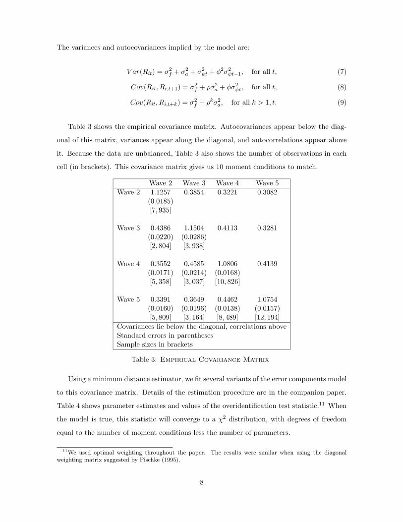
The variances and autocovariances implied by the model are:
V ar(Rit) = σ2f + σ2
a + σ2ψt + φ2σ2
ψt−1, for all t, (7)
Cov(Rit, Ri,t+1) = σ2f + ρσ2
a + φσ2ψt, for all t, (8)
Cov(Rit, Ri,t+k) = σ2f + ρkσ2
a, for all k > 1, t. (9)
Table 3 shows the empirical covariance matrix. Autocovariances appear below the diag-
onal of this matrix, variances appear along the diagonal, and autocorrelations appear above
it. Because the data are unbalanced, Table 3 also shows the number of observations in each
cell (in brackets). This covariance matrix gives us 10 moment conditions to match.
Wave 2 Wave 3 Wave 4 Wave 5
Wave 2 1.1257 0.3854 0.3221 0.3082(0.0185)[7, 935]
Wave 3 0.4386 1.1504 0.4113 0.3281(0.0220) (0.0286)[2, 804] [3, 938]
Wave 4 0.3552 0.4585 1.0806 0.4139(0.0171) (0.0214) (0.0168)[5, 358] [3, 037] [10, 826]
Wave 5 0.3391 0.3649 0.4462 1.0754(0.0160) (0.0196) (0.0138) (0.0157)[5, 809] [3, 164] [8, 489] [12, 194]
Covariances lie below the diagonal, correlations aboveStandard errors in parenthesesSample sizes in brackets
Table 3: Empirical Covariance Matrix
Using a minimum distance estimator, we fit several variants of the error components model
to this covariance matrix. Details of the estimation procedure are in the companion paper.
Table 4 shows parameter estimates and values of the overidentification test statistic.11 When
the model is true, this statistic will converge to a χ2 distribution, with degrees of freedom
equal to the number of moment conditions less the number of parameters.
11We used optimal weighting throughout the paper. The results were similar when using the diagonalweighting matrix suggested by Pischke (1995).
8
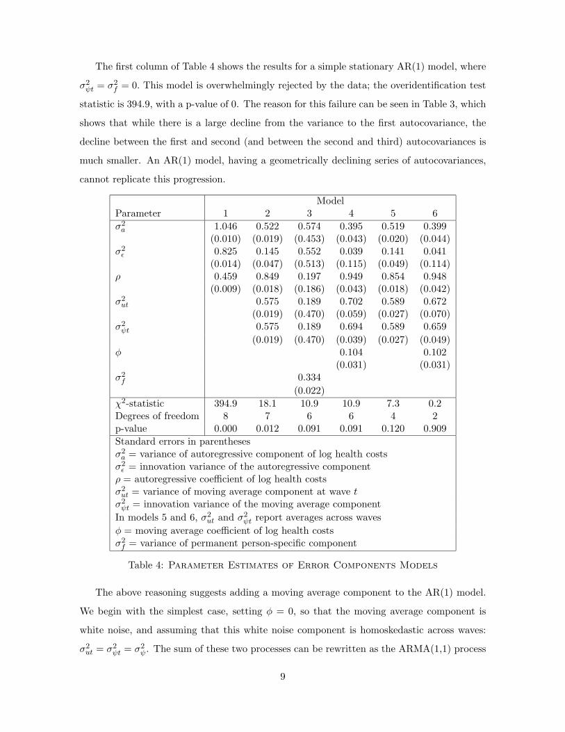
The first column of Table 4 shows the results for a simple stationary AR(1) model, where
σ2ψt = σ2
f = 0. This model is overwhelmingly rejected by the data; the overidentification test
statistic is 394.9, with a p-value of 0. The reason for this failure can be seen in Table 3, which
shows that while there is a large decline from the variance to the first autocovariance, the
decline between the first and second (and between the second and third) autocovariances is
much smaller. An AR(1) model, having a geometrically declining series of autocovariances,
cannot replicate this progression.
ModelParameter 1 2 3 4 5 6
σ2a 1.046 0.522 0.574 0.395 0.519 0.399
(0.010) (0.019) (0.453) (0.043) (0.020) (0.044)σ2ǫ 0.825 0.145 0.552 0.039 0.141 0.041
(0.014) (0.047) (0.513) (0.115) (0.049) (0.114)ρ 0.459 0.849 0.197 0.949 0.854 0.948
(0.009) (0.018) (0.186) (0.043) (0.018) (0.042)σ2ut 0.575 0.189 0.702 0.589 0.672
(0.019) (0.470) (0.059) (0.027) (0.070)σ2ψt 0.575 0.189 0.694 0.589 0.659
(0.019) (0.470) (0.039) (0.027) (0.049)φ 0.104 0.102
(0.031) (0.031)σ2f 0.334
(0.022)
χ2-statistic 394.9 18.1 10.9 10.9 7.3 0.2Degrees of freedom 8 7 6 6 4 2p-value 0.000 0.012 0.091 0.091 0.120 0.909
Standard errors in parenthesesσ2a = variance of autoregressive component of log health costsσ2ǫ = innovation variance of the autoregressive componentρ = autoregressive coefficient of log health costsσ2ut = variance of moving average component at wave tσ2ψt = innovation variance of the moving average component
In models 5 and 6, σ2ut and σ2
ψt report averages across waves
φ = moving average coefficient of log health costsσ2f = variance of permanent person-specific component
Table 4: Parameter Estimates of Error Components Models
The above reasoning suggests adding a moving average component to the AR(1) model.
We begin with the simplest case, setting φ = 0, so that the moving average component is
white noise, and assuming that this white noise component is homoskedastic across waves:
σ2ut = σ2
ψt = σ2ψ. The sum of these two processes can be rewritten as the ARMA(1,1) process
9
studied by Feenberg and Skinner.12 Estimates for this model are reported in the second
column of Table 4. The overidentification test statistic is 18.1, implying a considerably
better fit than the AR(1). Given that we have only 7 degrees of freedom, however, the model
is still rejected, with a p-value of 0.012.
A common error components model of wages (see Abowd and Card, 1989, for example)
includes a permanent person-specific effect, fi, and allows the moving average component of
wages to follow an MA(1) process instead of white noise. Columns 3 and 4 of Table 4 show
the effects of these two changes. These models fit the data better than the AR(1) with white
noise,13 although they are still rejected at the 10% level.
Allowing for heteroskedasticity in ψit across waves also improves goodness of fit. Such
heteroskedasticity could reflect the wave-to-wave variation that exists in the survey questions
used to generate the health cost measure. Results from this model are shown in column 5
of Table 4.14 Given that the empirical variance of health costs changes significantly from
wave to wave, allowing for heteroskedasticity significantly improves the fit; the χ2 statistic
falls to 7.3.15 This model is not rejected at the 10% level. One last attempt to improve the
fit of the model allows the moving average component of health costs to be an MA(1) with
heteroskedastic innovations. Estimates are in column 6. The model does fit the data better,
but introduces two additional parameters, leaving us with only two degrees of freedom.
For the exercises in Section 5 below, we use the AR(1)-plus-homoskedastic white noise
time series model. Although the heteroskedastic models provide better fits, much of this
heteroskedasticity likely reflects wave-specific differences in the wording of questions, rather
than changing health cost risk over time. The homoskedastic model is also more parsimonious,
and is more easily compared to other studies. Fortunately, the parameters ρ, σ2a, and σ2
ut
seem reasonably stable across models 2, 4, 5 and 6, so that all of the models have similar
time series implications.
12See Hamilton (1994, p. 393) for a derivation.13In both cases, moving from the AR(1)-plus-homoskedastic white noise model (model 2) to the more general
model (model 3 or 4) reduces the χ2 statistic by 7.2. Under the null that model 2 is correct, these decreasesin χ2 statistics are both distributed χ2(1) (as models 3 and 4 both have one more parameter than model 2),so that the observed decrease of 7.2 has a p-value of 0.007.
14The reported estimates and standard errors for σ2
ψt and σ2
ut are averages across waves.15Moving from model 2 to model 5 adds three parameters and reduces the χ2 statistic by 10.8. With a
χ2(3) distribution, this decrease has a p-value of 0.013.
10

4 Cross-Sectional Distribution
For the risk-averse, the possibility of catastrophic health care costs may be a matter of
great concern. This means that when modelling the cross-sectional distribution of health
care costs, special attention must be given to fitting the far right tail. Moreover, even if one
prefers a nonparametric approach, the scarce data of the upper tail might require employing
a parametric model. We thus proceed in two steps, considering first the upper tail, and then
the entire distribution.
4.1 The Upper Tail
Previous studies have identified two statistical models for the upper tail of the health cost
distribution. Feenberg and Skinner (1994) use the lognormal distribution. This implies that
the conditional density function for large health costs, f(.), is
f(lnhc| lnhc ≥ lnhcL) =1
1 − Φ([lnhcL − µ]/σ)φ([lnhc− µ]/σ)
1
σ, (10)
where Φ and φ are the standard normal cdf and pdf, respectively; µ and σ are the mean and
standard deviation of the untruncated distribution; and hcL is the truncation point used to
define the upper tail. Rust and Phelan (1997) use the Pareto distribution, which has the
density
g(hc|hc ≥ hcL) = γhcγLhc−(1+γ). (11)
A change of variables shows that if hc has a Pareto distribution, its logarithm has an expo-
nential distribution:
g(lnhc| lnhc ≥ lnhcL) = γe−γ[lnhc−lnhcL]. (12)
The two models can be compared formally with the likelihood ratio test developed by
Vuong (1989) and extended by Rivers and Vuong (2002). Consider a sample of log health
costs of size N . Let LN (µN , σ2N ) and LN (γN ) denote the maximized sample log-likelihoods for
the truncated normal and exponential models, respectively. Suppose that 1N ω
2N consistently
estimates the variance of 1N [LN (µN , σ
2N )−LN (γN )], the mean log-likelihood difference. Since
the two models in question are strictly non-nested, it follows from Vuong (Theorem 5.1) and
Rivers and Vuong (Theorems 1 and 3) that the adjusted statistic
11

DN ≡ N−1/2
(1
ωN[LN (µN , σ
2N ) − LN (γN )] − 1
)(13)
will converge in distribution to a standard normal variable if the two models are equivalent.
On the other hand, if the truncated normal model better represents the data generating
process for log health costs, DN will converge to infinity and the estimated p-value will
converge to 0; if the exponential model is better, DN will converge to negative infinity and
the p-value to 1.
To perform the Vuong test, we treat our panel of health cost data as a single cross
section.16 To account for the effects of age, gender, marital status, income, wave, and health
insurance type, we repeat the linear regression shown in Table 2, compute the residuals,
and add back the mean.17 The first column of Table 5 presents parameter estimates, log-
likelihoods, and p-values of the Vuong statistic DN for the top decile of this modified cross
section. Recalling the discussion above, the p-value of 0.266 shown on the bottom line of
Table 5 suggests that the two models are roughly equivalent.
EntireItem Sample Wave 5
90th percentile of log health costs (lnhc0.9) 8.41 8.47Number of observations in top decile (N) 3,490 1,220Truncated NormalµN -24.13 -24.29
(0.2224) (0.1567)σ2N 21.70 22.31
(0.3117) (0.1275)Log-likelihood -1,938.2 -707.8
ExponentialγN 1.56 1.52
( 0.0264 ) (0.0436)Log-likelihood -1,938.7 -707.4
p-value of the Vuong test statistic DN 0.2664 0.7925
Standard errors in parentheses
Table 5: Parameter Estimates and Log-Likelihood Values for the Top Decile
16Although a household’s health care costs are correlated across waves, we can calculate the likelihood valuesas if the observations were independent—the Vuong test is valid even if both of the competing models aremisspecified. The variance estimate ω2
N must be calculated, however, in a way that captures this correlation;see the companion paper for details.
17We also controlled for the conditioning variables by breaking the data into cells by age, marital status, andhealth insurance type and repeating the analysis of this section for each cell. The companion paper containsthese detailed results, which are qualitatively similar to the results presented here.
12

Recall that the wave 5 data may do a better job of capturing nursing home costs, which
could skew the health cost distribution to the right. We therefore repeat the conditioning
regression (with wave variables omitted) and the estimation with the wave 5 data alone. Per-
haps not surprisingly, the second column of Table 5 shows that the fatter-tailed exponential
model better fits the wave 5 data, although the difference is not significant at standard levels.
4.2 The Entire Cross Section
Although the Pareto and lognormal models fit the upper tail of the empirical health cost
distribution equally well, the overall cross section allows us to discriminate between the two.
Figure 1 shows the cross-sectional distribution for the entire sample. Once the effects of
the conditioning variables have been removed, the empirical distribution is fairly close to
lognormal.
Figure 1: Distribution of Health Care Costs
This conclusion is reinforced by the first four columns of Table 6, which show that the
“standard” Pareto distribution, the one estimated on the entire cross section (with hcL set
to the sample minimum), is markedly inferior to the “standard” lognormal model in every
dimension. Even if we could somehow extend a Pareto model of the top decile to the entire
13
health cost distribution, we would have difficulty incorporating it into the time series models
estimated in section 3.18 While a stationary ARMA process with normal innovations (that is
common across households) will generate a normally-distributed cross section, to our knowl-
edge there is no closed-form innovation distribution for log health costs that generates an
exponential cross section. These concerns lead us to abandon the Pareto as a model of the
overall cross section.
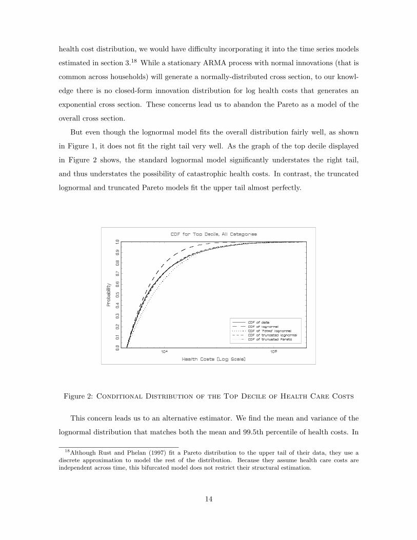
But even though the lognormal model fits the overall distribution fairly well, as shown
in Figure 1, it does not fit the right tail very well. As the graph of the top decile displayed
in Figure 2 shows, the standard lognormal model significantly understates the right tail,
and thus understates the possibility of catastrophic health costs. In contrast, the truncated
lognormal and truncated Pareto models fit the upper tail almost perfectly.
Figure 2: Conditional Distribution of the Top Decile of Health Care Costs
This concern leads us to an alternative estimator. We find the mean and variance of the
lognormal distribution that matches both the mean and 99.5th percentile of health costs. In
18Although Rust and Phelan (1997) fit a Pareto distribution to the upper tail of their data, they use adiscrete approximation to model the rest of the distribution. Because they assume health care costs areindependent across time, this bifurcated model does not restrict their structural estimation.
14
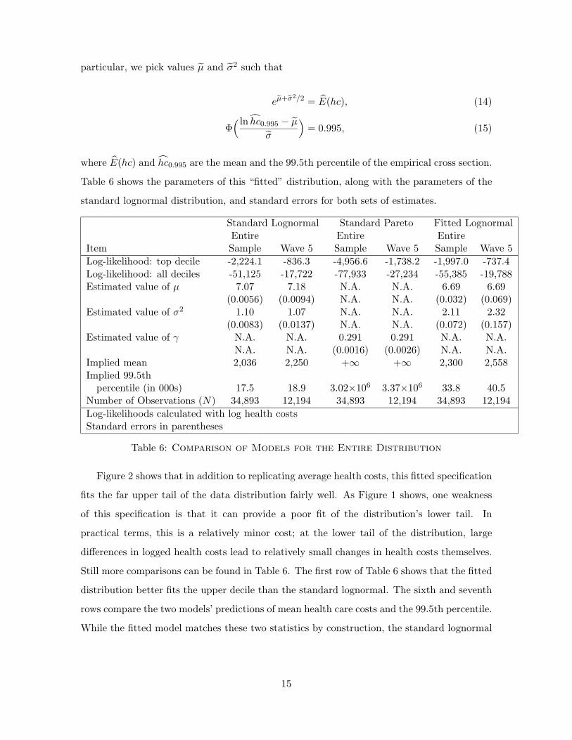
particular, we pick values µ and σ2 such that
eµ+σ2/2 = E(hc), (14)
Φ( ln hc0.995 − µ
σ
)= 0.995, (15)
where E(hc) and hc0.995 are the mean and the 99.5th percentile of the empirical cross section.
Table 6 shows the parameters of this “fitted” distribution, along with the parameters of the
standard lognormal distribution, and standard errors for both sets of estimates.
Standard Lognormal Standard Pareto Fitted LognormalEntire Entire Entire
Item Sample Wave 5 Sample Wave 5 Sample Wave 5
Log-likelihood: top decile -2,224.1 -836.3 -4,956.6 -1,738.2 -1,997.0 -737.4Log-likelihood: all deciles -51,125 -17,722 -77,933 -27,234 -55,385 -19,788Estimated value of µ 7.07 7.18 N.A. N.A. 6.69 6.69
(0.0056) (0.0094) N.A. N.A. (0.032) (0.069)Estimated value of σ2 1.10 1.07 N.A. N.A. 2.11 2.32
(0.0083) (0.0137) N.A. N.A. (0.072) (0.157)Estimated value of γ N.A. N.A. 0.291 0.291 N.A. N.A.
N.A. N.A. (0.0016) (0.0026) N.A. N.A.Implied mean 2,036 2,250 +∞ +∞ 2,300 2,558Implied 99.5th
percentile (in 000s) 17.5 18.9 3.02×10⁶ 3.37×10⁶ 33.8 40.5Number of Observations (N) 34,893 12,194 34,893 12,194 34,893 12,194
Log-likelihoods calculated with log health costsStandard errors in parentheses
Table 6: Comparison of Models for the Entire Distribution
Figure 2 shows that in addition to replicating average health costs, this fitted specification
fits the far upper tail of the data distribution fairly well. As Figure 1 shows, one weakness
of this specification is that it can provide a poor fit of the distribution’s lower tail. In
practical terms, this is a relatively minor cost; at the lower tail of the distribution, large
differences in logged health costs lead to relatively small changes in health costs themselves.
Still more comparisons can be found in Table 6. The first row of Table 6 shows that the fitted
distribution better fits the upper decile than the standard lognormal. The sixth and seventh
rows compare the two models’ predictions of mean health care costs and the 99.5th percentile.
While the fitted model matches these two statistics by construction, the standard lognormal
15

model often misses by a large margin.19 For the full sample, the standard lognormal implies
a 99.5th percentile that is half of what is seen in the data.20
A good model of the health cost distribution should be able to accurately measure the
welfare losses associated with health cost uncertainty. We therefore conduct a simple numeri-
cal experiment, where we estimate the welfare loss that a household with certain health costs
would experience if its health costs became uncertain. Assuming that lifetime utility is given
by V (A − hc), where V (.) is a value function and A is assets, we compute welfare losses by
comparing E(V (A − hc)) to V (A − E(hc)), using three different health cost distributions:
the empirical cross section; the standard lognormal; and the fitted lognormal. The results of
the experiment, which we describe in some detail in the companion paper, show that while
the fitted lognormal model and the empirical distribution generate similar welfare losses, the
welfare losses generated by the standard lognormal are much smaller. By understating the
risk of a catastrophic shock, the standard lognormal model understates the welfare cost of
health care uncertainty.
Finally, it is useful to compare the parameter estimates in Table 6 to the lognormal esti-
mates for the top decile shown in Table 5. The lognormal parameters estimated for the top
decile are quite different from the lognormal parameters estimated for the full distribution,
and are unlikely to fit the overall distribution very well. For example, the lognormal parame-
ters shown on the first column of Table 5 imply that mean health care costs are less than one
cent. All of these factors suggest that in terms of simultaneously matching both the overall
distribution and its upper tail, the fitted lognormal provides the best approximation.
19The mean implied by the fitted distribution, $2,300, is below the raw data mean of $2,600, because thefitted distribution is estimated with data that have been purged of income, wave and demographic effects.Because this filtering reduced the variance of log health costs without changing their mean, health coststhemselves are lower.
20When the data are bottom-coded with Hubbard et al.’s rules (see footnote 8), the standard lognormalmodel fits the upper tail much better, and, moreover, is very close to the alternative model we develop here.Our alternative model, however, is estimated mostly from the upper tail, and does not rely on bottom-codingdecisions.
16

5 Lifetime Health Cost Risk
5.1 The Annual Stochastic Process
The stochastic process for log health costs can be found by combining the time series
model estimated in Section 3 with a model for the distribution of log health cost innovations.
Unfortunately, the error components model that we estimate does not allow us to back out
an empirical distribution of log health cost innovations, because the sum of an AR(1) and an
MA process is not a Markov process. On the other hand, the lognormal model in Section 4
implies that the innovations are normal: if log health costs are normally distributed in the
cross-section and follow a stationary ARMA process, then the innovations to that process
must be normally distributed.21 Therefore, our preferred model of the health cost process
combines the AR(1)-plus-homoskedastic white noise time series model (discussed in Section 3)
with the fitted lognormal approximation of the cross section (discussed in Section 4).
An important limitation of this model is that the health cost data which it fits consist
of two-year averages. In order to make our results comparable to other papers, we fit an
annual model of log health costs to the data, using the Method of Simulated Moments. By
simulating a large number of health cost histories at a one-year frequency and aggregating
them into two-year data, we can find the summary statistics for two-year data implied by any
set of one-year parameters. We estimate the model by finding the parameter values that come
closest to replicating the mean and 99.5th percentile of health costs (as in Section 4), and
the first three autocorrelations of the log health cost residuals, found in the HRS/AHEAD
data. Details of our approach are in the companion paper. This “fitted lognormal” model is
analogous to the fitted lognormal model derived above. We also estimate a one-year analog
to the standard lognormal model, where we match mean log health costs and the variance
and first three autocovariances of the log health cost residuals. Comparing the two models
gives a sense of how failing to match the upper tail may lead to an understatement of health
cost risk.
Table 7 presents estimates of the annual health cost process for the entire data set. As
21More generally, if households share a common stationary and ergodic health cost process, the unconditionalhealth cost distribution for an individual household must equal the cross-sectional distribution across thepopulation. A rigorous discussion of the necessary conditions for a stationary cross-sectional distribution canbe found in Stokey and Lucas (1989). (Although the discussion there is couched in terms of Markov processes,one can derive stationary cross-sectional distributions for each component of our model, and then consider thesum.)
17
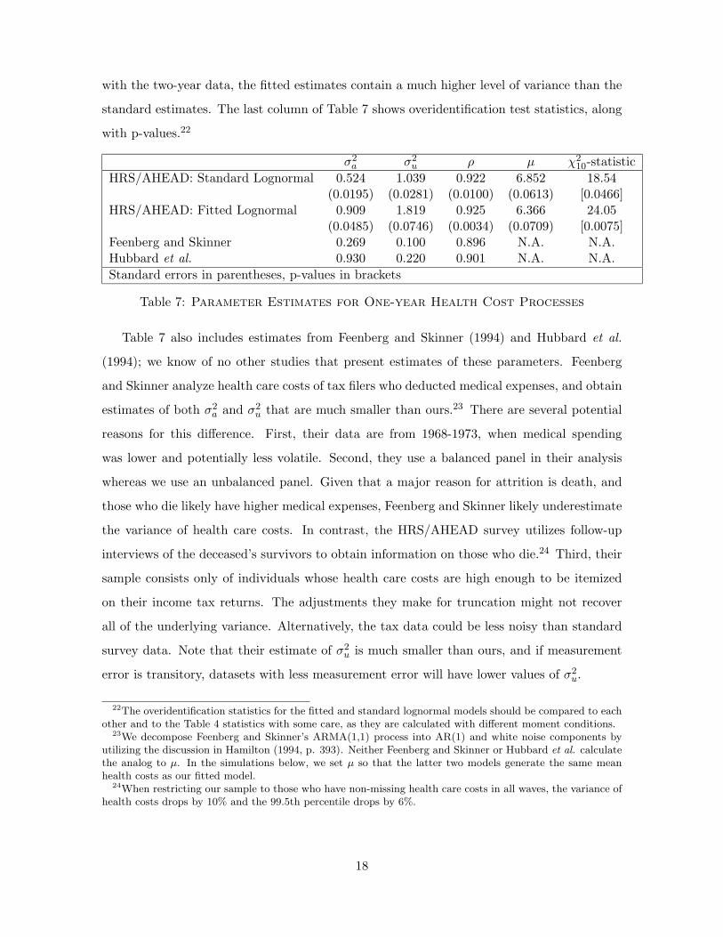
with the two-year data, the fitted estimates contain a much higher level of variance than the
standard estimates. The last column of Table 7 shows overidentification test statistics, along
with p-values.22
σ2a σ2
u ρ µ χ210-statistic
HRS/AHEAD: Standard Lognormal 0.524 1.039 0.922 6.852 18.54(0.0195) (0.0281) (0.0100) (0.0613) [0.0466]
HRS/AHEAD: Fitted Lognormal 0.909 1.819 0.925 6.366 24.05(0.0485) (0.0746) (0.0034) (0.0709) [0.0075]
Feenberg and Skinner 0.269 0.100 0.896 N.A. N.A.Hubbard et al. 0.930 0.220 0.901 N.A. N.A.
Standard errors in parentheses, p-values in brackets
Table 7: Parameter Estimates for One-year Health Cost Processes
Table 7 also includes estimates from Feenberg and Skinner (1994) and Hubbard et al.
(1994); we know of no other studies that present estimates of these parameters. Feenberg
and Skinner analyze health care costs of tax filers who deducted medical expenses, and obtain
estimates of both σ2a and σ2
u that are much smaller than ours.23 There are several potential
reasons for this difference. First, their data are from 1968-1973, when medical spending
was lower and potentially less volatile. Second, they use a balanced panel in their analysis
whereas we use an unbalanced panel. Given that a major reason for attrition is death, and
those who die likely have higher medical expenses, Feenberg and Skinner likely underestimate
the variance of health care costs. In contrast, the HRS/AHEAD survey utilizes follow-up
interviews of the deceased’s survivors to obtain information on those who die.24 Third, their
sample consists only of individuals whose health care costs are high enough to be itemized
on their income tax returns. The adjustments they make for truncation might not recover
all of the underlying variance. Alternatively, the tax data could be less noisy than standard
survey data. Note that their estimate of σ2u is much smaller than ours, and if measurement
error is transitory, datasets with less measurement error will have lower values of σ2u.
22The overidentification statistics for the fitted and standard lognormal models should be compared to eachother and to the Table 4 statistics with some care, as they are calculated with different moment conditions.
23We decompose Feenberg and Skinner’s ARMA(1,1) process into AR(1) and white noise components byutilizing the discussion in Hamilton (1994, p. 393). Neither Feenberg and Skinner or Hubbard et al. calculatethe analog to µ. In the simulations below, we set µ so that the latter two models generate the same meanhealth costs as our fitted model.
24When restricting our sample to those who have non-missing health care costs in all waves, the variance ofhealth costs drops by 10% and the 99.5th percentile drops by 6%.
18
Hubbard et al. use cross-sectional data from the 1977 National Health Care Expenditures
Survey and the 1977 National Nursing Home Survey to estimate the total cross-sectional
variance of health care costs. Their estimated total, σ2a + σ2
u, is smaller than either of our
estimates, perhaps because their data are 20 years older than ours and lack the health costs
of those who died.25 Because Hubbard et al. allocate total variance between σ2a and σ2
u
largely on the basis of Feenberg and Skinner’s estimates, they also attribute much more of
the cross-sectional variance to the autoregressive component, σ2a, than we do.
5.2 Lifetime Health Cost Risk
Using the stochastic processes described in Table 7, we can estimate the lifetime health
cost risk that households face. In particular, we simulate 30-year health cost sequences for
1 million households. Each household begins at age 64 with a draw of ai64 from its invariant
distribution and then realizes a 30-year sequence of innovations, {ǫit, uit}94t=65. Adding µ to
these sequences of shocks and exponentiating yields a health cost history for each individ-
ual.26 To measure lifetime health care costs, we discount this sequence back to age 65, using
an annual interest rate of 3% and age- (but not health- or health cost-) specific mortality
adjustments. Holding all other variables fixed, we then recompute the sequence with one or
both of the age-65 innovations, (ǫi65, ui65), set to zero. The differences between the various
discounted sequences give the lifetime effects of the age-65 innovations.
Table 8 shows the effects of the age-65 innovations on age-65 and lifetime health care
costs. The first column of Table 8 shows results for the standard lognormal model, while
the second column shows results for the fitted lognormal model. When the AR(1) and
white noise innovations are considered together, the fitted lognormal implies that the lifetime
cost variation induced by the age-65 shocks has a standard deviation of $12,870. This is
considerably larger than the standard deviation of the age-65 variation, $7,990, indicating
that persistence in health care costs is important. Moreover, the variation induced by the
AR(1) innovation, ǫi65, has a lifetime standard deviation of $10,440 and an age-65 standard
25Although Hubbard et al. do not explicitly match extreme health cost events when estimating theirvariance, their bottom-coding decisions largely attenuate this problem. When we use Hubbard et al.’s bottom-coding rule (see footnote 8), the cross-sectional variance of the standard lognormal model increases from 1.56to 2.35.
26To restore the age effects that have been removed from the stochastic processes in Table 7, we let µ varyby age, using the coefficients given in Table 2. We have not attempted to account for other differences withinor across individuals.
19

deviation of $2,840. Although transitory shocks generate most of the cross-sectional and
short-term variance, it is the persistent shocks (reflecting chronic conditions) that generate
most of the lifetime health cost risk. Turning to catastrophic shocks, we find that under our
fitted lognormal model, 1% of the population will receive an age-65 shock to lifetime health
costs of at least $43,500, and 0.1% will receive a shock of at least $124,700. This is much
more risk than is implied by the standard lognormal model.
HRS/AHEAD: HRS/AHEAD: Feenberg- HubbardStandard Fitted Skinner et al.
Standard Deviation of Age-65 Health Care Costs (in $000s)Due to ǫi65 1.19 2.84 0.61 1.59Due to ǫi65 + ui65 3.63 7.99 1.01 2.29
Standard Deviation of Lifetime Health Care Costs (in $000s)Due to ǫi65 5.58 10.44 3.74 8.70Due to ǫi65 + ui65 6.57 12.87 3.82 8.86
Change in Lifetime Health Care Costs Due to ǫi65 + ui65 (in $000s)99th percentile 23.9 43.5 11.8 31.799.9th percentile 54.7 124.7 19.9 71.1
Total Increase in Lifetime Costs Given a $1 Increase in Age-65 CostsMedian ratio $1.55 $1.61 $3.01 $3.82
Table 8: Effects of Age-65 Shocks on Lifetime Health Care Costs
The amount of health cost risk implied by our estimates is considerably higher than
that found by Feenberg and Skinner. Redoing the simulations with Feenberg and Skinner’s
parameter values, we find that the lifetime cost effects have a standard deviation of $3,820,
of which $3,740 is attributable to the AR(1) innovation. When Hubbard et al.’s parameter
values are used, the standard deviations rise to $8,860 and $8,700.
Lastly, we compute the total increase in lifetime health care costs associated with a $1
increase in health care costs at age 65. For each simulated household we divide the change
in lifetime costs generated by ǫi65 + ui65 by the change in age-65 costs caused by the same
two shocks. Taking the median of this ratio, we find that a $1 shock to current health care
costs leads to somewhere between $1.55 and $1.61 of total lifetime health care costs. Using
Feenberg and Skinner’s parameter values and our methodology, we find that a $1 health cost
shock today leads to $3.01 of lifetime health costs.27 Using Hubbard et al.’s parameter values,
the corresponding figure is $3.82. Given that our estimates attribute a much smaller fraction
27When mortality risk is omitted from the simulations, the lifetime effect rises from $3.01 to $3.62. This isvery close to Feenberg and Skinner’s reported value of $3.65.
20

of the variance to the autoregressive component, it is not surprising that health cost shocks
have less persistent effects in our model.
6 Conclusion
Using data from the Health and Retirement Survey and the Assets and Health Dynamics
of the Oldest Old survey, this paper presents estimates of the stochastic process that deter-
mines the distribution and dynamics of health care costs. We find that the data generating
process for log health costs is well represented as the sum of an AR(1) and a white noise
process. We also find that the innovations to the log health cost process can be modelled
with a normal distribution. However, the variance of this innovation distribution and the
mean for the overall process should be adjusted so that the model matches the mean and the
99.5th percentile of the empirical health cost distribution. This fitted lognormal distribution
matches the right tail of the health cost distribution much better than the standard lognor-
mal model, which understates the probability of catastrophic health costs. Simulating this
fitted distribution reveals significant catastrophic health cost risk: in any given year 0.1% of
households suffer a shock that costs at least $125,000 over their lifetimes. The risk implied
by our model is considerably more than is implied by previous estimates.
We conclude by pointing out six caveats to our analysis. First, to the extent that our
data suffer from classical measurement error, our estimates will overstate the transitory vari-
ation in health care costs. Second, because the initial sample excluded those who were in
nursing homes, we may be understating health care costs from this source, leading us to
underestimate both the level and variability of health care costs. The third problem is that
the quantity of health care services consumed is, to some extent, a choice. This means that
households can reduce their health care costs by reducing the amount of medical services
they consume. Fourth, low income, low wealth households have access to Medicaid, making
health care services very inexpensive. While we have conditioned our estimates on several
factors, including income and health insurance type, we might not have completely removed
these two effects. Fifth, those with high health care costs often die shortly after their health
cost shock. Because they die so soon, people who suffer from massive health cost shocks face
less risk of being financially destitute (Pauly, 1990). Finally, we have assumed that health
costs have no effect on income. However, it is likely to be the case that many of the shocks
21

that affect a household’s health care costs also affect its members’ ability and/or willingness
to work.
References
[1] Abowd, J., and David Card (1989), “On the Covariance Structure of Earnings andHours Changes”, Econometrica, 57(2), 411-445.
[2] Blau, D., and D. Gilleskie (2000), “A Dynamic Structural Model of Health Insuranceand Retirement”, manuscript.
[3] Crystal, S., R. Johnson, J. Harman, U. Sambamoorthi, and R. Kumar (2000),“Out-of-Pocket Health Care Costs Among Older Americans”, Journal of Gerontology
Series B: Psychological Sciences and Social Sciences, 55(1), S51-62.
[4] Dynan, K., J. Skinner, and S. Zeldes (2002), “The Importance of Bequests and Life-Cycle Saving in Capital Accumulation: A New Answer”, American Economic Review,92(2), 274-278.
[5] Eichner, M., M. McClellan, and D. Wise (1998), “Insurance or Self-Insurance?Variation, Persistence, and Individual Health Accounts”, in D. Wise, ed., Inquiries in
the Economics of Aging, 19-45.
[6] Employee Benefit Research Institute (1999), Health Benefits Databook, EBRI-ERF.
[7] Feenberg, D., and J. Skinner (1994), “The Risk and Duration of Catastrophic HealthCare Expenditures”, The Review of Economics and Statistics, 76(4), 633-647.
[8] Federal Interagency Forum on Aging-Related Statistics (2000), Older Ameri-
cans 2000: Key Indicators of Well-Being, U.S. Government Printing Office, available athttp://www.agingstats.gov/chartbook2000/default.htm.
[9] French, E., and J. Jones (2003), “The Effects of Health Insurance and Self-Insuranceon Retirement Behavior”, manuscript.
[10] French, E., and K. Kamboj (2003), “The Effect of Health Insurance on Health Costsand Health Care Utilization of the Elderly”, Economic Perspectives, 26(3), 60-72.
[11] Hamilton, J. (1994), Time Series Analysis, Princeton University Press.
[12] Hubbard, R., J. Skinner, and S. Zeldes (1994), “The Importance of PrecautionaryMotives in Explaining Individual and Aggregate Saving”, Carnegie-Rochester Series on
Public Policy, 59-125.
[13] National Center for Health Statistics (1999), Health and Aging Chartbook, Hy-attsville, MD.
[14] Palumbo, M. (1999), “Uncertain Medical Expenses and Precautionary Saving Nearthe End of the Life Cycle”, Review of Economic Studies, 66(2), 395-421.
[15] Pauly, M. (1990), “The Rational Non-Purchase of Long Term-Care Insurance”, Journal
of Political Economy, 98(1), 153-168.
22
[16] Pischke, J-S (1995), “Measurement Error and Earnings Dynamics: Some EstimatesFrom the PSID Validation Study”, Journal of Business & Economics Statistics, 13(3),305-314.
[17] Rivers, D., and Q. Vuong (1997), “Model Selection Tests for Nonlinear DynamicModels”, Econometrics Journal, 5, 1-39.
[18] Rust, J. and C. Phelan (1997), “How Social Security and Medicare Affect RetirementBehavior in a World of Incomplete Markets”, Econometrica, 65(4), 781-831.
[19] Selden, T., K. Levit, J. Cohen, S. Zuvekas, J. Moeller, D. McKusick, and
R. Arnett (2001), “Reconciling Medical Expenditure Estimates from the MEPS andNHA, 1996”, Health Care Financing Review, 23(1), 161-178.
[20] Stokey, N., and R. Lucas (1989), Recursive Methods in Economic Dynamics, HarvardUniversity Press.
[21] Vuong, Q. (1989), “Likelihood Ratio Tests for Model Selection and Non-nested Hy-potheses”, Econometrica, 57(2), 307-333.
23