UNIVERSITE LIBRE DE BRUXELLES

Ecole Polytechnique de Bruxelles

IRIDIA - Institut de Recherches Interdisciplinaires

et de Developpements en Intelligence Artificielle

On the Design and Implementation of anAccurate, Efficient, and Flexible Simulator for

Heterogeneous Swarm Robotics Systems

Carlo PINCIROLI

Promoteur de These:Prof. Marco DORIGO

Co-Promoteur de These:Prof. Mauro BIRATTARI

These presentee en vue de l’obtention du titre deDocteur en Sciences de l’Ingenieur

Annee academique 2013-2014

Abstract

Swarm robotics is a young multidisciplinary research field at the in-tersection of disciplines such as distributed systems, robotics, artifi-cial intelligence, and complex systems. Considerable research effort hasbeen dedicated to the study of algorithms targeted to specific problems.Nonetheless, implementation and comparison remain difficult due to thelack of shared tools and benchmarks. Among the tools necessary to en-able experimentation, the most fundamental is a simulator that offersan adequate level of accuracy and flexibility to suit the diverse needs ofthe swarm robotics community. The very nature of swarm robotics, inwhich systems may comprise large numbers of robots, forces the designto provide runtimes that increase gracefully with increasing swarm sizes.

In this thesis, I argue that none of the existing simulators offers satis-factory levels of accuracy, flexibility, and efficiency, due to fundamentallimitations of their design. To overcome these limitations, I presentARGoS—a general, multi-robot simulator that currently benchmarks asthe fastest in the literature.

In the design of ARGoS, I faced a number of unsolved issues. First,in existing simulators, accuracy is an intrinsic feature of the design. Forsingle-robot applications this choice is reasonable, but for the large num-ber of robots typically involved in a swarm, it results in an unacceptabletrade-off between accuracy and efficiency. Second, the prospect of swarmrobotics spans diverse potential applications, such as space exploration,ocean restoration, deep-underground mining, and construction of largestructures. These applications differ in terms of physics (e.g., motiondynamics) and available communication means. The existing general-purpose simulators are not suitable to simulate such diverse environ-ments accurately and efficiently.

To design ARGoS I introduced novel concepts. First, in ARGoS ac-curacy is framed as a property of the experimental setup, and is tunableto the requirements of the experiment. To achieve this, I designed thearchitecture of ARGoS to offer unprecedented levels of modularity. Theuser can provide customized versions of individual modules, thus as-signing computational resources to the relevant aspects. This featureenhances efficiency, since the user can lower the computational cost of

i

unnecessary aspects of a simulation.To further decrease runtimes, the architecture of ARGoS exploits the

computational resources of modern multi-core systems. In contrast toexisting designs with comparable features, ARGoS allows the user todefine both the granularity and the scheduling strategy of the paralleltasks, attaining unmatched levels of scalability and efficiency in resourceusage.

A further unique feature of ARGoS is the possibility to partition thesimulated space in regions managed by dedicated physics engines run-ning in parallel. This feature, besides enhancing parallelism, enablesexperiments in which multiple regions with different features are simu-lated. For instance, ARGoS can perform accurate and efficient simula-tions of scenarios in which amphibian robots act both underwater andon sandy shores.

ARGoS is listed among the major results of the Swarmanoid project.1

It is currently the official simulator of 4 European projects (ASCENS,2

H2SWARM,3 E-SWARM,4 Swarmix5) and is used by 15 universitiesworldwide. While the core architecture of ARGoS is complete, exten-sions are continually added by a community of contributors. In particu-lar, ARGoS was the first robot simulator to be integrated with the ns3network simulator,6 yielding a software able to simulate both the physicsand the network aspects of a swarm. Further extensions under devel-opment include support for large-scale modular robots, construction of3D structures with deformable material, and integration with advancedstatistical analysis tools such as MultiVeStA.7

1http://www.swarmanoid.org/2http://ascens-ist.eu/3http://www.esf.org/activities/eurocores/running-programmes/eurobiosas/

collaborative-research-projects-crps/h2swarm.html4http://www.e-swarm.org/5http://www.swarmix.org/6http://www.nsnam.org/7http://code.google.com/p/multivesta/

ii

To my family

iii

Acknowledgements

I would like to express my deep gratitude to Prof. Marco Dorigo for giv-ing me the opportunity to work at IRIDIA, a laboratory with a livelyand stimulating environment. Marco’s constant support in the devel-opment of my work has been a precious source of motivation. Duringmy years at IRIDIA, Marco’s advice and criticism have been crucial toshape me as a researcher and as a person. I look up to Marco for hisability to lead, and for his sharp vision of future research directions.

I would also like to thank Dr. Mauro Birattari. The interactionsI had with Mauro during my doctoral studies exceeded his role as asupervisor. While teaching me how to be a good researcher, Mauro hasalso helped me to accept my limits and strengthen my abilities. I amproud to call Mauro a friend.

I also wish to thank Prof. Andrea Roli for the interesting and pleasantdiscussions we had. I cherish our collaborations, and I consider them aprecious occasion to learn and grow as a researcher.

I wish to thank the people who helped me design and develop AR-GoS: Frederick Ducatelle, Gianni Di Caro, Istvan Fehervari, MichaelAllwright, and Vito Trianni. Without their feedback, criticism, andcontributions, ARGoS probably would not exist.

IRIDIA is a fantastic working environment populated by a variegatedgang of remarkable characters. My doctoral period has spanned three‘generations’ of iridians. While people joined and left, IRIDIA’s uniquemixture of professionalism, creativity, and fun remained intact. Thanksto Hughes Bersini and Thomas Stutzle for contributing to the creationof the IRIDIA gang and for constantly nurturing it.

Among those of the ‘old’ (pre-Swarmanoid) generation, I wish tothank Anders Lyhne Christensen, Bruno Marchal, Christos Ampatzis,and Elio Tuci for the interesting discussions and the beers we shared.

Among those of the Swarmanoid generation, I first wish to thankRehan O’Grady. His excellent vision and communication skills havebeen an invaluable source of inspiration for me.

I would also like to thank Manuele Brambilla, Giovanni Pini, EliseoFerrante, Marco Montes de Oca, and Arne Brutschy. You are a pleasureto work with and great friends.

v

I also wish to thank Alexandre Campo, Alessandro Stranieri, An-tal Decugniere, Francesco Sambo, Matteo Borrotti, Navneet Bhalla,Nithin Mathews, Prasanna Balaprakash, and Yara Khaluf for havingcontributed to making IRIDIA the unique place it is.

I want to thank the ‘new’ generation of iridians, who is taking goodcare of IRIDIA’s traditions of great research and epic fun: Anthony An-toun, Dhananjay Ipparthi, Gaetan Podevijn, Gabriele Valentini, Gian-piero Francesca, Giovanni Reina, Leonardo Bezerra, Leslie Perez Caceres,Lorenzo Garattoni, Roman Miletitch, Tarik Roukny, and Touraj Soley-mani.

Special thanks to my officemates: Ali Turgut and Kiyohiko Hattori.It was great fun to chat and share the office with you.

I am grateful to Muriel Decreton, for her kindness and our chats, andto Carlotta Piscopo, for always finding a way to make me smile.

During my doctoral studies, I had the luck to participate to the AS-CENS project. This project gave me the opportunity to interact withextraordinary researchers whose interests and backgrounds are differ-ent from mine, motivating me to widen my knowledge and follow newpaths. I wish to thank in particular Prof. Martin Wirsing for his con-stant support and encouragement. I would also like to thank Prof. UgoMontanari, Prof. Franco Zambonelli, Michele Loreti, Rosario Pugliese,Francesco Tiezzi, Nora Koch, Matthias Holzl, Mariachiara Puviani, andAnnabelle Klarl for the stimulating and pleasant discussions we had.

I would also like to thank Prof. Francesco Mondada, Michael Bonani,and their group at EPFL for their essential role in providing the robotswe use at IRIDIA, and for keeping them in working condition.

I would like to thank Rachael for having dedicated time and patienceto reading and correcting my English, both written and oral, on a dailybasis. Your love and encouragement make my life complete.

My final thought is to thank my family, to which I dedicate this work.You gave me the freedom and the means to choose my own path, andsupported my choices unconditionally and lovingly.

vi

Contents

Abstract i

Acknowledgements v

Contents vii

List of Figures ix

1 Introduction 11.1 Problem Statement . . . . . . . . . . . . . . . . . . . . . . 41.2 Thesis Structure and Research Contributions . . . . . . . . 51.3 Other Scientific Contributions . . . . . . . . . . . . . . . . 7

2 Context and State of the Art 92.1 Context: Swarm Robotics Systems . . . . . . . . . . . . . 102.2 Simulation of Swarm Robotics Systems . . . . . . . . . . . 27

3 The ARGoS Architecture 433.1 Requirements . . . . . . . . . . . . . . . . . . . . . . . . . 433.2 Modularity . . . . . . . . . . . . . . . . . . . . . . . . . . . 443.3 Entity Indexing . . . . . . . . . . . . . . . . . . . . . . . . 523.4 Multiple Physics Engines . . . . . . . . . . . . . . . . . . . 533.5 Multiple Threads . . . . . . . . . . . . . . . . . . . . . . . 55

4 Achieving Flexibility 614.1 Requirements . . . . . . . . . . . . . . . . . . . . . . . . . 614.2 Modules as Plug-ins . . . . . . . . . . . . . . . . . . . . . . 634.3 Arbitrary Interactions among Modules . . . . . . . . . . . 69

5 Efficiency Assessment 775.1 Experimental Setup . . . . . . . . . . . . . . . . . . . . . . 785.2 2D-Dynamics Physics Engine . . . . . . . . . . . . . . . . . 805.3 Results with Other Physics Engines . . . . . . . . . . . . . 83

vii

6 Validation 876.1 Flocking . . . . . . . . . . . . . . . . . . . . . . . . . . . . 886.2 Cooperative Navigation . . . . . . . . . . . . . . . . . . . . 926.3 Task Partitioning in Cooperative Foraging . . . . . . . . . 946.4 Discussion . . . . . . . . . . . . . . . . . . . . . . . . . . . 98

7 Team Recruitment and Delivery in a HeterogeneousSwarm 1017.1 Introduction . . . . . . . . . . . . . . . . . . . . . . . . . . 1017.2 Related Work . . . . . . . . . . . . . . . . . . . . . . . . . 1037.3 Methodology . . . . . . . . . . . . . . . . . . . . . . . . . . 1047.4 Hardware . . . . . . . . . . . . . . . . . . . . . . . . . . . . 1057.5 Active Shelters . . . . . . . . . . . . . . . . . . . . . . . . . 1077.6 Scalability Assessment . . . . . . . . . . . . . . . . . . . . 115

8 Conclusions and Future Work 125

A Other Scientific Contributions 129A.1 Swarm Robotics . . . . . . . . . . . . . . . . . . . . . . . . 129A.2 Boolean Network Robotics . . . . . . . . . . . . . . . . . . 137A.3 Other Publications . . . . . . . . . . . . . . . . . . . . . . 138

B Compiling and Installing ARGoS 141B.1 Licensing . . . . . . . . . . . . . . . . . . . . . . . . . . . . 141B.2 Downloading ARGoS . . . . . . . . . . . . . . . . . . . . . 141B.3 Compiling ARGoS . . . . . . . . . . . . . . . . . . . . . . . 142B.4 Using ARGoS from the source tree . . . . . . . . . . . . . 145B.5 Installing ARGoS from the compiled binaries . . . . . . . . 146

C An Example of ARGoS in Use 149C.1 The Robot Control Code . . . . . . . . . . . . . . . . . . . 149C.2 The Experiment Configuration File . . . . . . . . . . . . . 153

Bibliography 159

viii

List of Figures

3.1 The architecture of ARGoS. The white boxes correspond touser-definable plug-ins. . . . . . . . . . . . . . . . . . . . . . . 44

3.2 Screen-shots from different visualizations. (a) Qt-OpenGL;(b) POV-Ray. . . . . . . . . . . . . . . . . . . . . . . . . . . . 48

3.3 (a) The foot-bot; (b) The eye-bot. . . . . . . . . . . . . . . . . 50

3.4 Simplified pseudo-code of the main simulation loop of AR-GoS. Each ‘for all’ loop corresponds to a phase of the mainsimulation loop. Each phase is parallelized as shown in Fig-ure 3.5. . . . . . . . . . . . . . . . . . . . . . . . . . . . . . . . 55

3.5 The multi-threading schema of ARGoS is scatter-gather. Themaster thread (denoted by ‘m’) coordinates the activity ofthe slave threads (denoted by ‘s’). The sense+control, actand physics phases are performed by P parallel threads. Pis defined by the user. . . . . . . . . . . . . . . . . . . . . . . 56

3.6 Information flow in the various phases of the main simulationloop of ARGoS. The robot entities live in the global space.A controller and a set of sensors and actuators are associatedto each robot. (a) In the initial phase, robot sensors collectinformation from the global space. Subsequently, robot con-trollers query the sensors and update the actuators with thechosen actions to perform. (b) The chosen actions stored inthe actuators are executed, that is, the robot state is updated.At this point, positions and orientations have not been up-dated yet. (c) The physics engines calculate new positionsand orientations for the mobile entities under their responsi-bility. Collisions are solved where necessary. . . . . . . . . . . 57

4.1 A high-level diagram representing the required interactionsamong developers, users, and the ARGoS core. . . . . . . . . 62

4.2 A UML class diagram of the basic plug-in hierarchy in ARGoS. 64

ix

4.3 A UML class diagram of the ARGoS plug-in manager. In thisdiagram, I use the notation A ## B to express the string con-catenation operator of the C++ pre-processor. In the C++pre-processor, the expansion of a symbol X corresponds to itsdefinition, if the symbol was previously defined; otherwise itsexpansion corresponds to the symbol itself. Thus, A ## B isthe string resulting from the concatenation of the expansionsof A and B. . . . . . . . . . . . . . . . . . . . . . . . . . . . . . 67

4.4 A UML class diagram for an example problem of inter-modulecommunication. In this diagram, two entities must be addedto a physics engine. The entities and the physics engine areimplemented by three different developers, out of the ARGoScore. . . . . . . . . . . . . . . . . . . . . . . . . . . . . . . . . 70

5.1 A screen-shot from ARGoS showing the simulated arena cre-ated for experimental evaluation. . . . . . . . . . . . . . . . . 77

5.2 The different space partitionings (A1 to A16) of the environ-ment used to evaluate ARGoS’ performance (a screen-shot isreported in Figure 5.1). The thin lines denote the walls. Thebold dashed lines indicate the borders of each region. Eachregion is updated by a dedicated instance of a physics engine. 79

5.3 Average wall clock time and speedup for a single physicsengine (A1). Each point corresponds to a set of 40 experi-ments with a specific configuration 〈N,P, A1〉. Each exper-iment simulates T = 60 s. In the upper plot, points underthe dashed line signify that the simulations were faster thanthe corresponding real-world experiment time; above it, theywere slower. Standard deviation is omitted because its valueis so small that it would not be visible on the graph. . . . . . 80

5.4 Average wall clock time and speedup for partitionings A2 toA16. Each point corresponds to a set of 40 experiments with aspecific configuration 〈N,P, AE〉. Each experiment simulatesT = 60 s. In the upper plots, points under the dashed linesignify that the simulations were faster than the correspond-ing real-world experiment time; above it, they were slower.Standard deviation is omitted because its value is so smallthat it would not be visible on the graph. . . . . . . . . . . . 82

x

5.5 Average wall clock time and speedup for experiments with2D-kinematics engines and 3D-dynamics engines. Each pointcorresponds to a set of 40 experiments with a specific con-figuration 〈N,P, A16〉. Each experiment simulates T = 60 s.In the upper plots, points under the dashed line signify thatthe simulations were faster than the corresponding real-worldexperiment time; above it, they were slower. Standard devia-tion is omitted because its value is so small that it would notbe visible on the graph. . . . . . . . . . . . . . . . . . . . . . . 84

6.1 A screen-shot from the flocking validation experiments of Sec-tion 6.1. The robot with the yellow LEDs lit is the only oneaware of the target direction. . . . . . . . . . . . . . . . . . . 88

6.2 Results of the flocking validation experiments of Section 6.1.The plots on the left show the result obtained in simulation,while those on the right report the results in reality. Thecolored areas span the result distribution from the first tothe third quartile. Each plots reports the data obtained withthree different motion control strategies: HCS, ICS, and SCS.Refer to Section 6.1.2 for more details on the motion controlstrategies. . . . . . . . . . . . . . . . . . . . . . . . . . . . . . 89

6.3 Results of the validation experiments of Section 6.1. Theplots on the left show a comparison of the flocking order ob-tained in simulation and with real robots. The plot on theleft show a comparison of flocking accuracy. Each plot is com-posed of two stacked elements: the top element reports thedata, the second element reports the results of a Wilcoxonsigned-ranked test on the difference between simulated andreal-world data. . . . . . . . . . . . . . . . . . . . . . . . . . . 90

6.4 Setup of the validation experiments of Section 6.2. The pic-ture on the left shows the real arena in which the experimentswere conducted. The target locations the robots must visitare marked by dedicated robots. The diagram on the rightdepicts the equivalent simulated arena. The empty and filledcircles represent the target positions, and the camera marksthe location in which the picture on the left was taken. . . . . 93

6.5 Results of the validation experiments of Section 6.2. Thenavigation delay is the time necessary for a robot to reachthe target location. Here, the graph shows its average. . . . . 93

6.6 When the same speed is applied to the foot-bot treels, therobot does not cover a straight line, due to an asymmetry inthe construction of the treel motors. . . . . . . . . . . . . . . 95

xi

6.7 The throughput of object transportation in simulation withand without noise and on real robots. The top plot shows theinterquartile range (Q25–Q75) of the raw data; the bottomplot reports the results of a Wilcoxon signed-rank test on thedifference between simulation without noise and real robots,and simulation with noise and real robots. . . . . . . . . . . . 96

6.8 Positioning error of the foot-bots with respect to their targetlocation. I report both the data sampled from real robotexperiments and from the dead-reckoning model described inSection 6.3.3. . . . . . . . . . . . . . . . . . . . . . . . . . . . 97

7.1 The robot platforms I simulated for the experiments in thisstudy. (a) The foot-bot; (b) the eye-bot. . . . . . . . . . . . . 106

7.2 A schematic representation of the mathematical model de-scribed in Section 7.5.1 with three active shelters. . . . . . . . 107

7.3 Length of phase 2 in the simulations of the mathematicalmodel for different values of the decay period δ. . . . . . . . . 108

7.4 Results with the mathematical model presented in Section 7.5.1.The experiments are composed of three phases. In phase 1,two shelters are active. In phase 2 (starting at time T1), athird shelter is activated. In phase 3 (starting at time T3),shelter 2 is deactivated. The experiment ends at time T3.The length of each phase depends on the dynamics of thesystem. P1 and P2 account for the desired group size of eachshelter. Parameter δ corresponds to the decay period for theprobability to leave a shelter. . . . . . . . . . . . . . . . . . . 109

7.5 State transition logic for robots at each time step. InRange()and JustInRange() are functions returning true when therobot is within the communication range of a shelter, and hasjust entered it, respectively. Rand() is a function returning arandom number in U(0, 1). ji is the join probability for shelteri, li is the leave probability. State transition conditions arerepresented be the symbol C and a subscript. For example,Cin group→in group represents the conditions under which anaggregated robot will stay aggregated in its group in a singletime step. . . . . . . . . . . . . . . . . . . . . . . . . . . . . . 112

xii

7.6 Results with physically simulated robots following the behav-ior explained in Section 7.5.2. The experiments are composedof three phases. In phase 1, two shelters are active. In phase2 (starting at time T1), a third shelter is activated. In phase3 (starting at time T2), shelter 2 is deactivated. The experi-ment ends at time T3. The top plots shows a representativeexperimental sample in the pool of the 100 repetitions I ran.The middle plot reports the average system behavior. Thebottom plot shows the ratio between the current and the de-sired group size. . . . . . . . . . . . . . . . . . . . . . . . . . . 113

7.7 Snapshot from scalability experiments with physically simu-lated robots. Left: Simulation snapshot. Right: Abstractedrepresentation of this simulation snapshot—the gray intensitylevel of each square is proportional to the recruited group sizeof the correspondingly positioned shelter (i.e., to the numberof robots recruited by that shelter). . . . . . . . . . . . . . . 116

7.8 Scalability experiments testing the convergence and spread-ing properties of the system. Results are shown for two setsof experiments with 16 shelters (a) and 25 shelters (b). 80experimental runs per set of experiments. The top plots showthe behavior of the system in a single sample experiment thatI have selected. The grids of squares represent snapshots ofthe state of the system at given moments in time during thissample experiment. The gray intensity of each individualsquare corresponds to the number of mobile robots recruitedat that time by a single shelter. The min-max lines show thesize of the largest recruited group of mobile robots and thesize of the smallest recruited group of foot-bots at any givenmoment. The 1Q and 3Q lines show the inter-quartile rangeof the distribution of recruited group sizes among the shelters.The 1Q is the first quartile and shows the minimum recruitedgroup size once I discard the lowest 25% of groups. The 3Qline is the third quartile, and shows the maximum recruitedgroup size once I discard the highest 25% of the data. Thebottom plot shows the same data averaged over all 80 runs. . 118

7.9 Set of experiments testing the spreading property of the sys-tem. All experiments run with 9 shelters and 180 mobilerobots in a recruitment area consisting of a 3x3 shelter for-mation. Results are shown for two sets of experiments. Eachexperimental run lasts for 1,500 s. 20 experimental runs wereconducted for each set of experiments. Top plots in each setrepresent selected sample runs, while bottom plots representdata averaged over all 20 runs. For a more detailed explana-tion of the plots see previous caption from Figure 7.8. . . . . 119

xiii

7.10 Set of experiments testing the spreading property of the sys-tem. All experiments run with 9 shelters and 180 mobilerobots in a recruitment area consisting of a 3x3 shelter for-mation. Results are shown for two sets of experiments. Eachexperimental run lasts for 1,500 s. 20 experimental runs wereconducted for each set of experiments. Top plots in each setrepresent selected sample runs, while bottom plots representdata averaged over all 20 runs. For a more detailed explana-tion of the plots see previous caption from Figure 7.8. . . . . 120

7.11 Set of experiments on local perturbation. In these experi-ments, the propagation of the reset signal is limited to thedirect neighbors. Results are shown for two sets of experi-ments (a,b). 20 experimental runs were conducted for eachset of experiments. Each experimental run lasts 1,500 s. Topplots in each set represent selected sample runs, while bot-tom plots represent data averaged over all 20 runs. For amore detailed explanation of the plots see previous captionfrom Figure 7.8. . . . . . . . . . . . . . . . . . . . . . . . . . . 122

7.12 Set of experiments on local perturbation. In these experi-ments, the propagation of the reset signal is limited to thesecond-level neighbors (i.e., the direct neighbors of the directneighbors of the signal originator). Results are shown for twosets of experiments (a,b). 20 experimental runs were con-ducted for each set of experiments. Each experimental runlasts 1,500 s. Top plots in each set represent selected sam-ple runs, while bottom plots represent data averaged over all20 runs. For a more detailed explanation of the plots seeprevious caption from Figure 7.8. . . . . . . . . . . . . . . . . 123

xiv

Chapter 1

Introduction

Swarm robotics (Beni, 2005) is a scientific field that originated from col-lective robotics and swarm intelligence (Bonabeau et al., 1999; Dorigoet al., 2000; Dorigo and Birattari, 2007). With respect to collectiverobotics, swarm robotics shares the fundamental challenges, i.e., design-ing effective control strategies for large groups of autonomous robotsto perform complex tasks. With respect to swarm intelligence, swarmrobotics shares principles and methods to achieve coordination (Beni,2005): fully distributed control, local communication and sensing, andself-organization (Camazine et al., 2003).

The observation of natural swarm systems offers the primary motiva-tions to pursuing this line of research. Natural swarm systems display anumber of desirable properties, such as robustness to environmental per-turbations, individuals mistakes, and/or death of a part of the swarm;adaptability to new operational and environmental conditions; and scal-ability, that is, the ability to maintain the overall performance withinacceptable bounds for wide ranges of the swarm size (Sahin, 2005).

Since its origin in the 90’s, swarm robotics has been linked to re-search in natural swarm intelligence systems. Researchers have appliedmodels of natural swarm systems to robotic scenarios, either to pro-pose new algorithms based on the original model (Balch et al., 2006;Schmickl, 2011), or to validate the model itself (Balch et al., 2006; Gar-nier, 2011; Mitri et al., 2013). In the first case, natural swarm systemsserve as a basis to understand how an artificial swarm system of com-parable characteristics can be realized. Experiments typically assess theperformance of the artificial system, and do not consider the degree ofsimilarity of the behavior of the artificial system and its natural coun-terpart. Conversely, in the second case, swarm robotics systems areused as fully controllable models of their natural counterpart, and ex-periments are designed to confirm or negate a hypothesis on the naturalswarm system under study. As an example of the former case, Garnieret al. (2008) proposed an aggregation algorithm inspired by Jeanson

1

et al. (2005)’s study on cockroaches. Example works for the latter caseare Beckers et al. (1994)’s robot implementation of Deneubourg et al.(1990) ant clustering model, and Garnier et al. (2013)’s work on antroute construction.

In the last decade, the research scope has widened considerably. Be-sides the original scientific trend, a new trend has emerged that em-phasizes the engineering aspects of the design of swarm robotics sys-tems (Brambilla et al., 2013; Dorigo et al., 2014). The engineeringtrend finds its raison d’etre in the development of new approaches totackle problems whose current solution is either impractical, danger-ous, or non-existent (Hinchey et al., 2007). A few examples of long-term applications are power-line maintenance, unexploded ordnance re-moval, search-and-rescue in disaster areas, space exploration, construc-tion, deep-underground mining, underwater environment restoration,and nanosurgery.

Research in swarm robotics is still at an early stage. The path torealize artificial systems that match the performance of natural swarmsremains long and presents many open problems. To date, the majorachievements in this field consist of algorithms that tackle specific prob-lem instances. The performance of these algorithms strongly dependsupon the context in which they are developed (i.e., hardware capabilitiesand assumptions on the environment). Given this state of affairs, repro-ducing results and comparing algorithms is difficult, and this hindersthe development of the research field as a whole. Despite the impor-tance of this issue, little work has been devoted to a standardizationof the robot capabilities, and to the creation of common platforms forexperimentation.

In this thesis, I deal with the problem of simulating swarm roboticssystems. Simulation is a fundamental tool for experimentation in thisfield, and its importance often surpasses that of the robots themselves.Over the last decade, a wealth of different robots suitable for swarmrobotics has appeared. In addition to the classical two-wheeled robotssuch as the Jasmine1, the Alice (Caprari et al., 1998), and the e-puck(Mondada et al., 2006), new concepts for ground robots (e.g., the Kilobot(Rubenstein et al., 2012)), flying robots (e.g., the AR-Drone (Krajnıket al., 2011)), and self-assembling robots (e.g., the s-bot (Mondada et al.,2004)) have been introduced to study algorithms for several applications,such as distributed exploration, monitoring, and morphogenesis. How-ever, today’s main challenge remains the prohibitive cost of building andmaintaining dozens or hundreds of robots in working condition (Caoet al., 1997; Carlson et al., 2004). For this reason, swarm algorithmsare more easily prototyped and analyzed in simulation. Simulated ex-

1http://www.swarmrobot.org/

2

periments do not risk harming humans and robots. A simulator offerscontrollable and repeatable experimental conditions, which are vital toassess the performance of an algorithm. Additionally, simulations canbe repeated hundreds of times, thus enabling the fast and inexpensivecollection of large amounts of data for analysis. The very nature ofswarm systems pushes for experiments involving thousands of individ-uals, which are simply impossible with current hardware. Simulationcan also enable experiments with yet-to-be-built robots, thus providinginformation (i) to support the design of sensors and actuators, and (ii)to assess the CPU and memory requirements of the behaviors understudy. For all these reasons, in the typical development cycle of swarmalgorithms, experimentation with real robots is performed solely as afinal step to validate the simulated experiments.

Despite the central role that simulation plays in the design of swarmalgorithms, in the current state of the art no significant effort has beendevoted to the creation of a genuinely general-purpose simulator forswarm robotics. This is in striking contrast with other branches ofrobotics, such as humanoid, in which practical knowledge of establishedsimulators such as Gazebo (Koenig and Howard, 2004) is considered anasset to obtain a job.

The lack of a general simulator for swarm robotics is due to the factthat creating a dedicated tool is often considered an uninteresting, yetunavoidable, technical chore of the experimental activities. Differentlyfrom the case of humanoid robotics, the models involved in a swarm sim-ulation tend to be extremely simple. While the simulation of a humanoidrobot requires extensive knowledge of mechanics, the agents involved ina swarm are often represented as collections of interacting mass-less par-ticles. Thus, in the case of humanoid robotics, the effort required to cre-ate a personal, single-use simulator is significant; conversely, in the caseof swarm robotics, the effort is typically negligible. Consequently, thedesign challenges posed by a truly general-purpose simulator for swarmrobotics are considered too complex and time-consuming to motivateattention.

In this thesis, I argue that the creation of a general-purpose simulatoris a necessary step to support the development of swarm robotics. Inaddition to the mentioned necessity regarding reproducibility and com-parability of swarm algorithms, a general-purpose simulator acts as acommon ground to enable cooperation and sharing of code. This as-pect is key to create the premises to identify best practices—the basicbuilding block of any engineering approach. Moreover, the prospectiveapplications of swarm systems target complex scenarios, thus requiringadvanced tools that support the design, implementation, and analysis ofcomplex swarm behaviors. These requirements exceed the capabilitiesof any single-use simulator, and necessitate innovative, general-purpose

3

platforms.

1.1 Problem Statement

The main focus of this thesis is the design and implementation of asimulator for large-scale, heterogeneous swarm robotics systems. To beuseful, a simulator must provide four main features.

The first feature is support for a natural development cycle, to allowthe user to prototype solutions, measure their performance, and seam-lessly validate them onto real robots. In other words, a simulator mustintegrate a set of tools, thus forming a coordinated software ecosystemthat constitutes a productive development framework.

The second required feature is simulating accurately the dynamics ofthe robots and of the environment, as well as the interactions amongrobots and between the robots and the environment. The simulationmust consider the space-network nature of swarm robotics systems: Theagents composing these systems possess a body and move in the physi-cal space; while, at the same time, the agents communicate, forming anetwork. At any moment, the state of a swarm is the composition ofboth spatial and network aspects. Spatial aspects include linear/rota-tional momentum and applied forces; network aspects include topologyand exchanged messages. Spatial aspects are inherently continuous, andtheir dynamics over time are typically modeled by classical mechanics.Network aspects, on the other hand, are discrete and proceed in anevent-based fashion.

The third feature necessary for the simulation of a swarm derivesfrom the large-scale and distributed nature of swarm robotics systems.This requires efficient simulation techniques. In this thesis, efficiencycorresponds to a wise usage of computational resources that aims tominimize the duration of a simulation.

The fourth required feature is flexibility. In the context of this work,flexibility refers to the possibility for the user to add new features, suchas new robots, sensors, and actuators. A truly flexible simulator canexecute any kind of experiment, provided the right set of models.

Accuracy, efficiency, and flexibility are generally viewed as divergingrequirements. Reaching a satisfactory degree of accuracy often entailsemploying models with high computational costs, which negatively af-fects run-times and, thus, efficiency. Flexibility entails very abstractand general designs, often imposing constraints on the data structuresused to store the state of the simulated world. As a result, the benefitsderived from a flexible design might limit the type of allowed models(hindering accuracy) and offer little opportunity for optimization (lim-iting efficiency). A design that offers satisfactory levels of accuracy, ef-

4

ficiency, and flexibility is a challenging problem whose solution requiresnovel concepts.

1.2 Thesis Structure and Research Contributions

In the past 15 years, development tools for robotics have increased expo-nentially. In particular, simulators that target fairly general use cases,such as Gazebo (Koenig and Howard, 2004), Webots (Michel, 2004),and USARSim (Balakirsky and Messina, 2006), have been introduced.These simulators, while covering a wide range of requirements for singlerobot systems, fail to provide the necessary features when increasinglylarger-scale multi-robot systems are involved.

This thesis is situated in this gap, providing solutions to realize anaccurate, efficient, and flexible simulator for large-scale swarm roboticssystems. The result of my work is a multi-robot simulator called ARGoS(Autonomous Robots Go Swarming). ARGoS was the official robot sim-ulator of the EU-funded project Swarmanoid,2 and it is currently usedin four European projects: ASCENS,3 H2SWARM,4 E-SWARM,5 andSwarmix.6 ARGoS is open source (under the terms of the MIT license)and is being continually updated.7

In the rest of this section, I present an overview of this thesis structureand list the publications I produced during my Ph.D.

In Chapter 2, I frame this work within the related literature. Thechapter is divided into two sections. The first provides context, by(i) presenting long-term applications of swarm robotics and existinghardware platforms, and (ii) sketching approaches to design, modeling,analysis, and implementation. The second section in this chapter is areview of existing simulation approaches and tools.

In Chapter 3, I provide a high-level overview of the design of ARGoS.In Section 3.1, I discuss the main design requirements. In Section 3.2,I describe the structure of the ARGoS architecture. In Section 3.3 Iexplain how ARGoS organizes spatial data. In Section 3.4, I presentone of the most distinctive features of ARGoS: how the simulated spacecan be partitioned into multiple physics engines executed in parallel.In Section 3.5, I illustrate the parallelization of execution into multiplethreads. The work in this chapter was published in:

• C. Pinciroli, V. Trianni, R. O’Grady, G. Pini, A. Brutschy, M. Bram-billa, N. Mathews, E. Ferrante, G. Di Caro, F. Ducatelle, T. Stir-

2http://www.swarmanoid.org/3http://ascens-ist.eu/4http://www.esf.org/activities/eurocores/running-programmes/eurobiosas/

collaborative-research-projects-crps/h2swarm.html5http://www.e-swarm.org/6http://www.swarmix.org/7ARGoS can be downloaded at http://iridia.ulb.ac.be/argos/.

5

ling, A. Gutierrez, L. M. Gambardella, M. Dorigo. ARGoS: aModular, Multi-Engine Simulator for Heterogeneous SwarmRobotics. Proceedings of the IEEE/RSJ International Conferenceon Intelligent Robots and Systems (IROS 2011), pages 5027–5034.IEEE Computer Society Press, Los Alamitos, CA, 2011.

In Chapter 4, I detail the low-level aspects of the ARGoS implemen-tation. More specifically, I show how the high-level principles and ideaspresented in Chapter 3 are realized in practice.

In Chapter 5, I report the experimental activities I conducted toassess the efficiency of ARGoS. In Section 5.1, I introduce the experi-mental setup. In Section 5.2, I show the results obtained by partitioningthe simulated space with multiple instances of the default 2D-dynamicsengine. In Section 5.3, I report the results of analogous experiments per-formed with the default 3D-dynamics engine and 2D-kinematics engine.The work in this chapter was published in:

• C. Pinciroli, V. Trianni, R. O’Grady, G. Pini, A. Brutschy, M. Bram-billa, N. Mathews, E. Ferrante, G. Di Caro, F. Ducatelle, M. Birat-tari, L. M. Gambardella, M. Dorigo. ARGoS: a Modular, Par-allel, Multi-Engine Simulator for Multi-Robot Systems.Swarm Intelligence, 6(4):271–295, 2012.

In Chapter 6, I present three complex research experiments thatshowcase the features of ARGoS, and validate the simulated resultsthrough real experiments. In Section 6.1, I present an experiment inwhich a large swarm of mobile robots performs flocking according tothree different strategies. This work shows the validity of the sensor/ac-tuator models provided by ARGoS by default. This work was publishedin:

• E. Ferrante, A. E. Turgut, C. Huepe, A. Stranieri, C. Pinciroli,M. Dorigo. Self-Organized Flocking with a Mobile RobotSwarm: a Novel Motion Control Method. Adaptive Behav-ior, 20(6):460–477, 2012.

In Section 6.2, I illustrate the results of an experiment in which anemergent swarm behavior observed in simulation is confirmed by real-robot experiments. This work was published in:

• F. Ducatelle, G. Di Caro, A. Forster, M. Bonani, M. Dorigo,S. Magnenat, F. Mondada, R. O’Grady, C. Pinciroli, P. Retornaz,V. Trianni, L. M. Gambardella. Cooperative Navigation inRobotic Swarms. Swarm Intelligence, available online at http://link.springer.com/article/10.1007%2Fs11721-013-0089-4#page-1, 2013.

In Section 6.3.1, I focus on an experiment in which the standard modelsprovided by ARGoS were not able to capture the dynamics of the real

6

robot swarm. I show how the problem was identified, and how ARGoSwas extended to deal with the issue. This work was published in:

• G. Pini, A. Brutschy, C. Pinciroli, M. Dorigo, M. Birattari. Au-tonomous Task Partitioning in Robot Foraging: an Ap-proach Based on Cost Estimation. Adaptive Behavior, 21(2):118–136, 2013.

In Chapter 7, I report a set of experiments that involve two types ofrobots—the foot-bot and the eye-bot. In these experiments, the eye-botcoordinate the formation of multiple groups of foot-bots, which mustperform several tasks in parallel. This work was published in:

• C. Pinciroli, R. O’Grady, A. L. Christensen, M. Birattari, M. Dorigo.Parallel Formation of Differently Sized Groups in a RoboticSwarm. SICE Journal of the Society of Instrument and ControlEngineers, 52(3):213–226, 2013.

• R. O’Grady, C. Pinciroli, A. L. Christensen, M. Dorigo. Super-vised Group Size Regulation in a Heterogeneous RoboticSwarm. 9th Conference on Autonomous Robot Systems and Com-petitions (Robotica 2009). IPCB, Castelo Branco, Portugal, pages113-119, 2009.

• C. Pinciroli, R. O’Grady, A. L. Christensen, M. Dorigo. Self-Organised Recruitment in a Heterogeneous Swarm. 14thInternational Conference on Advanced Robotics (ICAR 2009). Pro-ceedings on CD-ROM, paper ID 176, 8 pages, 2009.

In Chapter 8, I conclude the thesis and discuss directions for futurework.

1.3 Other Scientific Contributions

Over the course of my doctorate, I have conducted a number of studiesnot directly related to the main topic of this thesis. These works touchseveral topics, and can be divided into two categories: swarm roboticsand Boolean network robotics. For a detailed list, refer to Appendix A.

7

Chapter 2

Context and State of the Art

The objective of this chapter is to provide a definition of the phrase‘general-purpose simulator’. The content is divided in two parts.

In Section 2.1, I focus on defining the scope of the expression ‘general-purpose,’ by providing a broad sketch of the most significant research inswarm robotics. The presentation is tailored to highlight those aspectsthat impact the design of a simulator and its role in the developmentprocess of artificial swarm systems.

The meaning of ‘general-purpose’ is partially linked to the longevityof a simulator design. To be successful, a design must overcome thechallenge of time accommodating the increasing complexity of futureuse cases. In Section 2.1.1 I list a number of long-term applications inwhich swarm-based solutions are envisioned. These applications exceedthe current capability of swarm algorithms. As such, they provide visionfor the challenges that are yet to be tackled, and establish a referencefor the requirements of simulator design.

A truly ‘general-purpose’ simulator is capable of supporting any kindof robot. In swarm robotics, the number of available robot types hasincreased considerably over the last ten years, currently comprising avery heterogeneous family of platforms. For the foreseeable future, thistrend is set to continue. However, it is possible to identify a numberof common capabilities any robot must offer to be suitable for swarmapplications. In Section 2.1.2, I briefly illustrate the current state-of-the-art in robot hardware, and encode the capabilities these robots share intoa reference robot architecture.

Integration is another aspect that contributes to the meaning of‘general-purpose’. A simulator constitutes the center of an ecosystemof software with diverse purposes, namely design, implementation, andmodeling.

In Section 2.1.3, I discuss the current approaches in the design ofswarm robotics systems, and emphasize the impact of these approacheson the primitive operations a simulator must offer.

9

In Section 2.1.4, I concentrate on the implementation of swarm algo-rithms. Enabling this phase of the development process is arguably themost important requirement a simulator must meet. The complexity ofswarm systems, however, poses peculiar implementation challenges thatfostered the advent of several programming languages based on diverseconcepts. In this section, I present the most significant advancements inprogramming languages for swarm robotics, and discuss the issues forsupporting them in a simulator.

The second part of this chapter, Section 2.2, deals with the currentstate of the art in the simulation of swarm systems.

Section 2.2.1 is dedicated to modeling techniques for swarm sys-tems. Because it is located at the intersection of many disciplines,swarm robotics lends itself to a multitude of modeling approaches. Inthis section, I argue that despite the wealth of modeling approaches,physics-based simulation remains an unavoidable technique, due to thegenerality of the approach, and the minimal assumptions upon which itrelies.

In Section 2.2.2, I present a number of traditional techniques to modelthe physics of individual robots, and provide an overview of the mostwidely used software packages for physics simulation.

Finally, in Section 2.2.3, I discuss the current state of the art in robotsimulation. I critically analyze the design of a number of simulators thateither enjoy wide acceptance, or provide innovative features that relateto the problem of simulating swarm systems.

2.1 Context: Swarm Robotics Systems

2.1.1 Long-Term Applications

Swarm robotics systems are envisioned for large-scale application sce-narios that require reliable, scalable, and autonomous behaviors. In thissection, I present a number of such scenarios in which swarm roboticsmight provide key solutions.

Power-line Maintenance

Power grids are arguably among the fundamental systems upon whichmost of our technology relies. Maintaining such systems in workingcondition is critical. Power grids are massively distributed systems scat-tered across large areas. Currently, maintenance and reparation requiresubstantial human intervention, and these tasks prove dangerous andexpensive (Elizondo et al., 2010).

In the last decade, the concept of smart grid has started to gain mo-mentum. Smart grids are envisioned as power distribution systems capa-ble of intelligent monitoring, control, and communication, in which hu-

10

man intervention is minimal (Allan, 2012). Solutions based on roboticsare essential to the realization of this vision. The large-scale nature ofpower grids naturally involves solutions that limit centralization and,instead, rely on swarm-based algorithms.

Swarms are envisioned to perform tasks such as monitoring, mapping,fault detection, and reparation (Elizondo et al., 2010; Allan, 2012). Forelevated power-lines, UAVs are beginning to be employed for monitoringand mapping activities, while specialized line rovers have performed mi-nor maintenance tasks (Elizondo et al., 2010). Advancements in roboticsfor underground power-lines have been limited to cable inspection (Al-lan, 2012).

Unexploded Ordnance Removal

Unexploded ordnance removal is a dangerous but necessary task to im-prove life conditions in post-conflict zones, and to facilitate the reuse ofland for living and cultivation (Habib, 2007).

The current approach to this task involves human specialists, who de-tect and remove the explosive material manually. While this approachis thorough and accurate, the process is very slow and highly danger-ous (Habib, 2007). To mitigate these issues, robots have been introducedto help human operators (Carpenter, 2013). This can be seen as a steptowards replacing humans with autonomous robots.

In the near future, robots could be employed to explore large areas,detect landmines, and report on their position. This task is made diffi-cult by the fact that reliably detecting landmines is currently an unsolvedchallenge, and that navigation on the uneven terrains where landminesare hidden is a slow and dangerous operation for robots (Habib, 2007).

Search-and-Rescue

Search-and-rescue is a scenario in which victims of an accident mustbe located and brought to safety. Dangers are present both for therescuers and the victims. The rescuers are exposed to hazardous andoften unknown environments, and must perform activities that mightendanger their lives as well as those of the victims.

To solve these problems researchers have started to study robotics-based solutions. The most typical incarnation of the search-and-rescuescenario involves a collapsed building whose topology is unknown. Therobots must spread, build a map, locate the victims, and bring them tosafety.

Countless variants of this scenario have since been introduced. Thesevariants differ in various aspects, such as the type of robots employed(flying, wheeled, insect-like), the type of environment (2D/3D), the na-ture of the interactions between the robot and the environment (e.g.,

11

whether the robots can modify the environment to remove obstacles, ornot). An international competition1 is held every year to showcase andcompare research advances.

Space Exploration

Future scenarios of space exploration involve activities such as coordi-nated observation, planet monitoring, and on-orbit self-assembly (Izzoet al., 2005). The size and complexity of the spacecraft involved inthese activities is limited by the cost of building and launching theminto space. Additionally, space environments are harsh, and our abilityto maneuver a spacecraft promptly to avoid damage decreases with itsdistance from us (Goldsmith, 1999).

The distributed nature of these scenarios, coupled with the technolog-ical limitations in the construction of the spacecraft are compelling spaceagencies to consider missions in which large groups of small-scale satel-lites cooperate. To realize this vision, NASA and ESA have launchedpioneering programs such as APIES (D’Arrigo and Santandrea, 2006)and ANTS (Curtis et al., 2000) to study methods for distributed au-tonomous coordination in space.

Collective Construction

The construction of large structures is an activity that currently requireshuman intervention and involves no automation. Statistics on fatal orserious accidents expose the high risk that construction entails (Li andPoon, 2013).

Autonomous robotics has the potential to offer solutions that coulddecrease accidents, increase efficiency, and enable construction projectsin locations that today would be considered too dangerous for humans.

Research in this field is exploring several multi-robot approachessuch as collective block deposition (Petersen et al., 2011), smart mate-rials (Fernandez and Khademhosseini, 2010), and self-assembling struc-tures (Werfel et al., 2006).

Deep-Underground Mining

Deep-underground mining is a problem whose importance is quickly ris-ing, due to the increasing scarcity of near-surface raw materials (Rubio,2012).

Direct human intervention is generally considered impossible due tothe extreme conditions of deep-underground environments—lack of oxy-gen, absence of light, need for complex supply mechanisms (Donoghue,2004).

1http://www.robocuprescue.org/

12

Autonomous robotics system have been proposed as a possible so-lution to perform this task (Green and Plumb, 2011; Huh et al., 2011;Green, 2012). The large environments in which the robots are expectedto act require highly parallel and distributed solutions, in which large-scale robot swarms act in a coordinated fashion.

Underwater Environment Exploration and Restoration

Underwater environment exploration (Aro, 2012) and restoration (Rinke-vich, 2005) are necessary tasks to cope with the large-scale and poten-tially catastrophic damages caused by bottom fishing, marine pollution,and climate change (Jackson et al., 2001; Knowlton and Jackson, 2008;C. Hongo, 2012). Restoration is currently performed by human divers,but this activity is both slow and dangerous.

The use of swarms of Autonomous Underwater Vehicles (AUV) isexpected to provide viable solutions to improve both the efficiency andthe safety of the restoration process.

Nanotechnologies

Nanorobotics is a futuristic branch of robotics that deals with machinesoperating at scales in the order of 10−6 m. The cost-effective productionof this kind of robots is an ambitious goal that requires major break-throughs in molecular manufacturing (Sivasankar and Durairaj, 2012).

Nanorobotics finds potential applications in medicine, to permit treat-ment of diseases that are currently incurable. Future applications of thistechnology include cancer treatment, gene therapy, treatment of brainaneurysm, and dentistry.

The limits imposed by the small scale of these robots and the pecu-liar characteristics of the environment in which they will operate (thehuman body) create novel and unexplored challenges for robot con-trol (Mavroidis and Ferreira, 2013). The low-resource and simplisticnature of swarm behaviors is likely to play an important role in thedevelopment of this technology.

Discussion

These application scenarios can be characterized according to severalaspects. For the design of a simulator, the most prominent are scale,heterogeneity, physical properties, and communication means.

Scale. Regarding scale, I refer to the fact that the size of the agentsinvolved (more precisely, their sensor and actuation range) is minusculewith respect to the size of the overall scenario. Effective solutions arelikely to require systems that involve large numbers of agents acting inparallel and in a coordinated fashion.

13

Heterogeneity. The complexity of the above application scenarios re-quires robots with specific abilities. To maintain a high level of per-formance while keeping the production cost of the swarm low, a viableapproach is to employ heterogeneous robot swarms, i.e., swarms com-posed of individuals specialized in a subset of the necessary tasks. Atthe simplest level, robots could be divided in two classes—sensing andacting. Sensing robots would be equipped with high-quality sensory de-vices, and their task would be primarily exploration, map-building, andmonitoring. Conversely, acting robots would feature effective devicesto modify the environment, e.g., defusing the explosives in unexplodedordnance removal.

Physical Properties. The third distinguishing feature of the aforemen-tioned application scenarios is the physical properties of the environ-ment and of the robots. For example, one could consider the way inwhich robots navigate in the environment. In power-line maintenance, infirst approximation, the motion along the power network can be consid-ered one-dimensional. In unexploded ordnance removal, motion is two-dimensional, and can be modeled through kinematics equations. Spaceexploration is inherently three-dimensional, and in first approximationthe agents can be modeled as point-masses. Motion in an underwaterenvironment is similarly three-dimensional, but fluid dynamics plays afundamental role. In construction tasks, navigating a three-dimensionalstructure requires mechanical models. Deep-underground mining occursin muddy and/or heavily littered 3D environments, which can be cap-tured by voxel-based models. Finally, the motion physics of nanosystemsis dominated by colloidal effects.

Communication Means. Finally, effective coordination in these sce-narios depends dramatically on the available communication means.For instance, WiFi is a possible solution in some variants of search-and-rescue scenarios, but is unusable in underwater environments; stig-mergy could be employed by the robots to mark already explored areasin unexploded ordnance removal, but it is not available in deep spaceexploration.

2.1.2 Swarm Robotics Hardware

Several robotics platforms have been used to study swarm robotics ap-plications. However, to date, no platform can be considered a standardin the field, due to heterogeneity of interests and requirements acrossthe research community.

In this section, I identify a number of basic capabilities that a robotmust offer to be eligible for swarm robotics applications. These capabil-

14

ities constitute a robot reference architecture that identifies the type ofmodels and architectures that best suit a simulator for swarm robotics.

Locomotion

The simplest approach to locomotion is a differential drive system thatemploys two wheels, each powered by an electric gear motor. This de-sign is employed by a large number of robots, such as the Jasmine2,the s-bot (Mondada et al., 2004), the e-puck (Mondada et al., 2006),the Alice (Caprari et al., 1998), the marXbot (Bonani et al., 2010), andthe r-one (McLurkin et al., 2013). The main advantages of wheel-baseddifferential-drive locomotion are (i) the simplicity of motion modelingand control, and (ii) the fact that motor encoders provide odometry in-formation without the need for additional devices. The major drawbackof wheel-based motion is its relatively high cost in terms of componentsand manufacturing. For this reason, in the design of the Kilobot, Ruben-stein et al. (2012) substituted wheels with vibration motors, which offerthe same differential-drive motion control at a much lower cost. How-ever, vibration motors do not provide odometry information, and posestrict constraints on the type of surfaces on which the robot can move.

Recent years have seen the introduction of a large number of afford-able flying robots. To date, the most successful design approach is thequad-rotor configuration. Quad-rotors are inexpensive to build, and easyto model and control (Mellinger and Kumar, 2011). Notable examples inthis category are Parrot’s low-cost commercial robot AR.Drone (Krajnıket al., 2011), and the open-source designs AeroQuad and ArduCopter.

Communication

The ability to communicate is a fundamental requirement in swarmrobotics, because it enables the interactions upon which self-organizationis built. The most common communication modality in swarm roboticsis one-to-many, in the sense that the data originating from a robotreaches multiple robots within a limited range. Frequently, upon receiv-ing data, a robot is able to detect the relative positioning of its origin.This modality goes under the name of situated communication (Støy,2001).

One way to implement one-to-many situated communication is throughvision, by using robots equipped RGB LEDs and cameras. Vision hasbeen used to convey the internal state of the robots (Christensen et al.,2008), their role in the swarm (Nouyan et al., 2008), and to indicatedocking slots in self-assembly (Christensen et al., 2007). Vision-basedcommunication is possible on many robotic platforms, such as the s-bot,

2http://www.swarmrobot.org/

15

the marXbot, and the e-puck.3 The primary advantage of vision is thesimplicity of its implementation, since colored-blob detection algorithmsare freely available in the open-source library OpenCV.4 The fundamen-tal weaknesses of vision are (i) the limited number of bits that can beexchanged per control step, (ii) the high computational cost of visionalgorithms, and (iii) the fact that the communication quality is heavilydependent on proper parameter calibration, which in turn depends onenvironmental light conditions.

The disadvantages of vision can be partially overcome through short-range wireless communication. Gutierrez et al. (2009) proposed an ex-tension board for the e-puck in which data is exchanged through infraredsignals. The board is equipped with 12 modules composed of infraredemitters and receivers. The modules can be controlled individually tosimultaneously send different messages. Through this board, robots canachieve a maximum bandwidth of 160 b/s for each module. The com-munication board of the marXbot, designed by Roberts et al. (2009),uses two different methods to exchange data and detect the sender. Totransmit data, a radio signal is used; the detection of the sender relieson the exchange of infrared signals. The maximum bandwidth of thisboard is 800 b/s. The principal flaw of these boards is the added cost perunit they entail. A simpler, low-cost, yet limited solution to this prob-lem has been used in the design of the Kilobot. This robot is equippedwith a single infrared transmitter/receiver module pointed downwardsat the floor. This system works under the assumption that the floor isreflective, and offers a theoretical maximum bandwidth of 9.6 kb/s.

Sensing

Sensing allows the robot to collect information about the environmentin which it operates, and about other robots.

Among the many devices mounted on swarm robots, one ubiquitousdevice is the proximity sensor. This type of sensor provides the robotwith spatial data concerning nearby obstacles and robots. In its sim-plest form, the proximity sensor can be used to avoid obstacles; morecomplex devices that provide long-range data can permit SimultaneousLocalization and Mapping (SLAM).

Proximity sensors can be implemented in several ways. An infraredproximity sensor is a combination of two devices: an infrared light emit-ter and an infrared light receiver. The sensor works exploiting the factthat the emitted infrared light is reflected back upon hitting an object.The sensor is capable of estimating the distance between the emitter andthe object by measuring the difference in voltage between the emitted

3Through a third party extension board.4http://opencv.org/

16

light beam (which is known to the device) and the received one (which ismeasured). These sensors are cheap and easy to integrate on any robot,but their measures typically display high levels of noise. Many robotsare equipped with infrared proximity sensors: the Alice, the e-puck, thes-bot, and the marXbot, to name a few. Ultrasound sensors work on asimilar principle, i.e., listening to the echo of an emitted sound wave.Ultrasound sensors have a longer range than infrared proximity sensors,but they are more expensive and their measures depend on the composi-tion of the objects upon which the sound waves bounce. Laser scannersare an option that ensures precise measurements, but their high costrenders them unattractive for swarm applications.

Cameras are another widespread sensing device. Camera sensorsare relatively inexpensive to include on a robot, and their versatilityjustifies the extra cost. As discussed, camera sensors enable color-basedcommunication. In addition, they can be used to detect objects andlandmarks, and to reconstruct geometric environmental features.

Robot swarms are often equipped with a diverse set of other sensors.Ground sensors allow robots to detect the features of the ground. In-frared sensors, such as those mounted on the e-puck and the marXbot,allow the robot to detect differences in the color of the ground. RFIDcards are also employed to achieve stigmergy5, by storing data on RFIDtags scattered through the environment (Johansson and Saffiotti, 2009).Light sensors are employed to provide the robots with a global gradient,marking in this way the position of an important location in the envi-ronment (O’Grady et al., 2005), and smoke sensors are used to estimatethe origin of a fire (Marjovi et al., 2009).

Assembly and Manipulation

While motion and communication are ubiquitous features in roboticsplatforms, the capability to assemble with kin robots or manipulateobjects is only present in a minority. However, these capabilities areoften mentioned among the most interesting a robotic swarm can offer,because they enable self-assembly (Groß and Dorigo, 2008; Patil et al.,2013), and collective construction (Petersen et al., 2011).

Self-assembling robots can be categorized in three families: lattice-based, chain-based, and mobile robot architectures (Yim et al., 2002).

In lattice-based architecture, the robots connect into regular pat-terns, such as cubic or hexagonal. Some examples of robots in this cat-egory are I-Cube (Unsal et al., 2001), Proteo (Yim et al., 2001), mole-

5Stigmergy is a form of indirect communication among members of a swarm. Typically,stigmergy occurs as a byproduct of the modifications individuals perform on the environment.These modifications affect the behavior of other individuals working on the same area. Theconcept of stigmergy was introduced by Grasse (1959) to explain the fundamental interactionsthat occur among ants during nest building.

17

cube (Mytilinaios et al., 2004), and ATRON (Jørgensen et al., 2004).These robots are equipped with multiple docking devices that form rigidstructures.

Chain-based architectures are capable of connecting into chain-like ortree-like structures. Differently from lattice-based architectures, chain-based architectures display articulation, allowing them to change the po-sition and orientation of each module dynamically. Prominent examplesof this family of robots are PolyBot (Yim et al., 2000), CONRO (Cas-tano et al., 2002), and M-TRAIN (Murata et al., 2002).

Mobile robot architectures are capable of locomotion and self-assembly.The robots falling into this category are able to form different types ofstructures. Two prominent examples exist: CEBOT (Fukuda, 1991),a heterogeneous collection of robotic modules with sensing and dock-ing capabilities; and the s-bot (Mondada et al., 2004), the first fullyautonomous robot platform capable of locomotion and reconfigurableself-assembly into arbitrary shapes.

Robotic hardware for collective construction is still at a very earlystage. The essential concerns that complicate the design of fully func-tional robots are the manipulation/deposition of construction material,and the navigation of partially assembled structures.

Early attempts to tackle these issues target the construction of 2Dstructures. Everist et al. (2004) have proposed a construction systemusing specially-designed blocks, and Werfel et al. (2006) achieved com-parable results using struts.

Research on 3D structures includes cooperative assembly by com-plex robots (Sellner et al., 2006; Stroupe et al., 2006), manipulating andmaneuvering over specialized blocks (Terada and Murata, 2008), andstrut-climbing robots that become part of the structure they build (De-tweiler et al., 2006). The first fully autonomous robotic architecture toachieve complex construction of three-dimensional structures is TER-MES (Petersen et al., 2011), which is based on an integrated design of apassive block and a robot capable of manipulating/depositing the blockand navigating the assembled structure.

Discussion

Robotic hardware for swarm applications is very diverse. A general-purpose simulator that encompasses this wide variety of hardware ar-chitectures must prove extremely flexible.

The main source of heterogeneity is the dynamics of these devices.Motion, as well as assembling and manipulation, are obtained in differentways depending on the hardware platform. The primary shared aspectamong all these platforms is the fact that swarms are formed by largenumbers of identical robots. Heterogeneity and large quantities of robots

18

are intertwined aspects. A large number of specialized robots is lessexpensive to build, and easier to study and control.

In addition, it is possible to model these systems in an optimizedway with tailored approaches. As it will be discussed in Section 2.2.3,this fact has promoted the creation of domain-specific simulators thatcombine accuracy and efficiency, at the cost of flexibility.

2.1.3 Swarm Robotics System Design

Designing effective swarm robotics systems is a complex task. This com-plexity is rooted in the fact that swarm robotics systems are located atthe intersection between several domains, with which swarm roboticssystems share requirements and open problems. First, swarm roboticssystems can be seen as an instance of distributed systems. In this per-spective, the design of swarm robotics systems aims to achieve effectiveparallelism, while dealing with asynchronous dynamics and stochastic-ity. Second, swarm robotics systems are expected to be autonomous, toadapt to changing environmental conditions, and to display robustnessto failure. All these requirements are typical of artificial intelligence.Third, the fundamental role of local interactions among the compo-nents of a swarm can be modeled as a complex network. Finally, swarmrobotics systems share the typical complications of classical robotics sys-tems (cost, energy efficiency, robustness, . . . ), with the added challengeof enabling mass production of large numbers of robots.

In all these domains individually, sound design approaches and en-gineering methodologies are currently under study. As a consequence,a general and universally accepted theory of swarm systems remainsundefined (Schweitzer, 2003). Such theory is expected to provide ananalytical framework to design and predict the behavior of a swarmrobotics system prior to its implementation. In particular, this theoryshould offer a solution to the problem of translating a swarm-level be-havior into individual-level behaviors.

Because of the lack of general-purpose methodologies, the design ofswarm robotics systems currently focuses on small-scale, specific appli-cation scenarios within a limited, well-defined scope. The result of thisactivity depends strongly on the experience and ingenuity of the de-signer, and success stories are difficult to generalize. The approachesto designing swarm behaviors can be categorized along many dimen-sions. Regarding the design of a simulator, three dimensions are partic-ularly important: who realizes the design, where the design abstractionis placed, and how the behaviors are structured.

19

Who is the Designer?

With regard to the first dimension, design approaches can be dividedinto manual and automatic.

In manual methods, the human designer works on the system directly.The designer studies ways to achieve self-organization by factorizing theproblem into simpler instances and identifying recurring patterns. Mostworks that take inspiration from natural swarms fall into this category.

Conversely, in automatic methods, the self-organizing behavior isthe result of an algorithm configured by the human designer to searchfor the solution that best fits the requirements. Thus, the designerworks on the system indirectly. Methods in the fields of reinforcementlearning (Sutton and Barto, 1998) and evolutionary robotics (Nolfi andFloreano, 2004) are typical examples of this category.

Manual and automatic methods have two important differences. First,in manual methods, the experience on the problem domain and the in-genuity of the designer strongly affect the quality of the final result; inautomatic methods, the quality of the result depends on the algorithmused—the experience of the designer is required more for configuringthe algorithm properly, rather than for the problem domain. Second,manual methods tend to yield solutions whose structure is easier to un-derstand, maintain, and modify with respect to those solutions foundwith automatic methods. On the other hand, automatic methods areusually better at finding unexpectedly good solutions, which would beerroneously discarded by a human designer.

Where is the Design Abstraction Placed?

With respect to the second dimension, i.e., where the design abstrac-tion is placed, design approaches can be categorized into top-down andbottom-up.

The top-down abstraction views the swarm as a unique entity. Atthis level, the designer assumes that the mechanisms for coordinationare given, and works directly on swarm-level mechanisms.

The bottom-up abstraction considers the swarm as a collection ofseparate components. The designer develops mechanisms to achievecooperation among the components in order to perform a task. In swarmrobotics, this means that the level of abstraction is placed at the levelof the individual robots.

The bottom-up approach is currently the most widespread and suc-cessful abstraction. This is due to the fact that a fundamental pre-requisite of the top-down abstraction is currently missing—a widely es-tablished formalism that describes the behavior of a large-scale swarmsystem. Until this issue is solved, effective modeling approaches to pre-dict swarm behaviors and tools/programming languages to implement

20

swarm-level behaviors will not be fully achievable. However, researchon implementing the top-down abstraction is active and a number ofinteresting results exist. These results are presented in Section 2.1.4.

How is the Behavior Structured?

With respect to the third dimension, design approaches can be cate-gorized into monolithic approaches, modular approaches, and virtualphysics.

Monolithic behaviors are self-contained and typically single-task-oriented.It is not possible to readily identify simpler components in this type ofbehaviors. Most swarm behaviors from the field of evolutionary roboticsfall into this category, as neural networks, the typical structure targetedin evolutionary robotics works, are difficult to analyze.

Modular systems, on the other hand, are explicitly factorized intointercommunicating components, organized in various ways. The mostwidespread approach to connect sub-behaviors is to consider them asnodes in a graph, in which arcs encode the condition under which a robotswitches from the current sub-behavior to another. In the literature, thisapproach goes under the name of Finite State Machine (FSM) (Minsky,1967). The type of condition associated to the arcs further qualifies thetype of FSM—for instance, if each arc is associated with a probabilisticcondition, it is called a probabilistic FSMs. A hierarchical organizationof the behavior, such as the subsumption architecture (Brooks, 1986),has also been proposed in the literature.

In virtual physics, the robots are imagined to be immersed in a virtualpotential field. This field is ‘virtual’ because it is derived by a robot fromsensor data. The robots move according to the forces that result fromthe potential field. This approach was introduced by Khatib (1986), andlater refined and extended by Reif and Wang (1999), and Spears et al.(2004).

The main difference between the modular and virtual physics meth-ods is that, in the former, the current swarm state is discrete, becauseit corresponds to the set of the behaviors of the robots; conversely, invirtual physics methods, the state of the system is continuous, as it corre-sponds to the state of the virtual potential. Thus, in a modular behavior,a state change corresponds to a behavior switch, by one or more robots;whereas, in a virtual physics behavior, a state change corresponds to the(dis)appearance of a ‘fold’ in the potential field. Furthermore, in mod-ular behaviors, self-organization is the result of the interaction amongthe current behaviors of each individual. Hence, the design process mustconsider the possible combinations of individual behaviors explicitly. Incontrast, the virtual potential metaphor expresses self-organization asthe implicit process of relaxation of the swarm system towards a state

21

of minimum virtual energy.For this reason, modular methods are a natural choice to structure

behaviors in which it is easy to identify discrete phases and/or events.Classical examples in the literature are foraging (Liu et al., 2007), chain-ing (Nouyan et al., 2008), and self-assembly (Christensen et al., 2007).Swarm behaviors such as task allocation (Gerkey and Mataric, 2004),pattern formation (Pinciroli et al., 2008) and flocking (Ferrante et al.,2013), characterized by a continuous swarm state, are more suitablytackled by virtual physics methods.

Discussion

A development framework for swarm robotics must support all of theabove design methods. The proposed categorization maps directly torequirements on the desired architecture of the framework.

To enable manual design methods, a framework must offer suitablefunctionality to inspect and analyze swarm behaviors. This functionalitycan be interactive or non-interactive. Interactive functionality is usuallyoffered by a Graphical User Interface (GUI), and allows for (i) inspectionof the robot states (e.g., current sensor readings), and (ii) modification ofthe course of an experiment, such as adding/removing/moving an object.Non-interactive functionality includes the possibility to run hundreds ofexperiments and collect statistics.

To enable automatic methods, the framework must be designed tobe integrated within other tools. For instance, in evolutionary robotics,the framework must allow the user to employ a neural network libraryas behavioral code, and give control of when an experiment must bestarted to the genetic algorithm.

The bottom-up abstraction requires the development framework toprovide primitives to control the devices of the individual robots. Thetop-down approach, on the other hand, requires functionality such ascommunication mechanisms that are transparent to the developer.

Regarding behavior structuring, the framework must offer (i) thecorrect primitives to interact with the robots, and (ii) the means tointegrate the behavior with external tools such as an FSM library.

2.1.4 Swarm Robotics System Implementation

One of the most difficult challenges for the implementation of swarmbehaviors for real applications is programming. The faceted nature ofswarm robotics systems admits multiple approaches to behavior pro-gramming.

Analogously to design approaches, one possible categorization of pro-gramming approaches is bottom-up and top-down. Bottom-up approaches

22

correspond to programming the behavior of each robot individually; top-down approaches allow the developer to program the swarm as a singleentity, translating the swarm-level program into instructions for eachindividual automatically.

Bottom-up Programming Approaches

To date, the bottom-up approach is the most widespread. The lackof general, top-down design methodologies often forces the developer tothink at the individual level. Thus, it is natural to translate a bottom-updesign into a bottom-up implementation.

Additionally, a large number of programming languages can be usedto implement robot behaviors in a bottom-up fashion. Virtually allrobots are natively programmed in C and offer a C API, making thislanguage a natural choice. On the downside, C forces the programmerto focus on low-level aspects such as memory management and cre-ation of basic data structures (e.g., linked lists and trees). Thus, manypractitioners prefer object-oriented languages such as C++ and (occa-sionally) Java, for the higher-level abstraction they offer and their largelibrary collection. Following the recent increase in computational poweravailable on robotic platforms, scripting languages have also startedto become a viable alternative. Among the many, Lua6 and Python7

are the most successful. Lua is a very simple and extensible script-ing language designed for low-memory embedded systems. Lua is idealas a low-resource extension language. Python, on the other hand, isa feature-rich, general-purpose scripting language employed for an ex-tensive variety of applications, including artificial intelligence and dataanalysis.

The bottom-up approach also includes popular middleware for robotics,such as ROS,8 OROCOS,9 and YARP.10 The purpose of this kind of mid-dleware is twofold: (i) providing high-level functions for procedures ofgeneral use, such as image analysis, pattern recognition, and mapping;and (ii) offering primitives to structure and compose complex behav-ioral code. Despite its advantages, this type of middleware has foundlittle success in the swarm robotics community, due to the relativelyhigh computational resources it requires, and the lack of primitives forreal-time and multi-robot coordination.

6http://www.lua.org/7http://www.python.org/8http://www.ros.org/9http://www.orocos.org/

10http://wiki.icub.org/yarp/

23

Top-down Programming Approaches

In the last ten years, the research community has started to study top-down approaches. This effort is motivated by the observation that mostof the development time in the bottom-up approach is spent implement-ing low-level, ad hoc communication and coordination procedures. Forthe success of the aggregate behavior, these procedures must prove ro-bust to failure and performance degradation in presence of a high num-ber of interactions per second. The top-down approach, on the otherhand, assumes the presence of dedicated mechanisms of coordinationand communication, thus allowing the developer to reason at the swarmlevel.

The first research efforts towards the top-down approach occurredin the sensor network community. An ample set of abstractions andprogramming languages has been proposed (Mottola and Picco, 2011),some of which have evolved into languages that target robotics applica-tions. To date, two languages offer the most interesting features: Protoand Meld.

Proto (Beal and Bachrach, 2006) is a language that emphasizes thespatial aspects of a computing network. In other words, Proto is alanguage that programs ‘spatial computers,’ that is, a collection of con-nected computing devices scattered in a physical space. The spatialcomputer is modeled as a continuous medium in which each point isassociated to a value, i.e., a field. The primitive operations of Protoact on this field. There are four types of operations: (i) point-wiseoperations, which are applied to each point in a field; (ii) restriction op-erations, which allow for the selection of a sub-field upon which a certainoperation is performed (a form of spatial if construct); (iii) feedbackoperations, which encode the notion of evolution over time, allowingthe developer to store state; and (iv) neighborhood operations, whichexpress the flow of information across the medium. Originally, Protowas designed for non-mobile networks. Bachrach et al. (2010) extendedthe language to include motion by adding the notion of density at anyposition in the medium. In this perspective, motion is implemented asa mass flow across the medium.

Meld (Ashley-Rollman et al., 2007, 2009) works from a top-down ap-proach by allowing the developer to specify a high-level, logic descriptionof what the swarm as a whole should achieve. The low-level (commu-nication/coordination) mechanisms that reify the high-level goals (i.e.,the how) are left to the language implementation and are transparentto the developer. For this reason, the syntax of Meld follows the declar-ative paradigm. The core concepts of the language are facts and rules.A fact encodes a piece of information that the system considers trueat a given time. A special kind of fact is an action, that encodes an

24

operation that a robot must perform on the environment. Rules havethe role of producing new facts, and are triggered as soon as their asso-ciated condition is met. Rules can entail side effects, such as falsifyingfacts in the knowledge base. The language automatically deletes factsthat have become false. A computation in Meld consists of applying thespecified rules progressively to produce all true facts, until no furtherproduction is possible. A powerful feature of the language is the pos-sibility to specify rules that work on a subset of the entire knowledgebase. In Meld parlance, these rules are called aggregates. Two types ofaggregates exist: (i) selection rules, that allow to single out an elementin the input fact set (e.g., the fact with the maximum value), and (ii)computation rules, that perform a computation over the input fact set(e.g., the sum of all the fact values).

Proto and Meld are two very different solutions for the top-downdevelopment approach.

One important point on which these languages differ is in the man-agement of the underlying network topology. The continuous mediumabstraction of Proto does not allow for explicit representation of thenetwork topology, nor to refer to individual robots in the swarm. Incontrast, in Meld, the topology of the network is represented explicitly,and the language can express rules involving specific robots. In fact, theimplementation of Meld imposes the distribution of facts across robots,and, by design, each true fact is stored in a single robot. If a rule requiresfacts known by different robots, the robot executing the rule requests thefact base of the robot that owns the necessary fact. To make communi-cation possible, every robot R stores a fact neighbor(R,N) for each robotN in its neighborhood. This feature is desirable in applications such asmodular robotics and self-assembly, in which the relative positioning ofrobots often affects the overall behavior.

Another important difference between Meld and Proto is their syntaxand semantics. Meld follows the declarative programming paradigm.Meld rules are expressed as logic statements, and computation occursby iteratively applying rules, producing new facts. Thus, in a non-trivialMeld program, it is difficult to predict the possible effects of a certainrule solely from the program source. Debugging a Meld program requirescarefully following the chain of productions. This issue is exacerbated bythe fact that facts might be deleted as a result of robot motion, makingit difficult to reproduce erroneous executions. In contrast, Proto is afunctional language, with a syntax similar to LISP. Proto statementsrepresent the computation as a composition of mathematical functions.For a human developer, Proto statements are readable and the executionof the program is usually predictable from the source code.

A desirable feature in any programming language is compositionality,i.e., the possibility to organize instructions into functions and libraries.

25

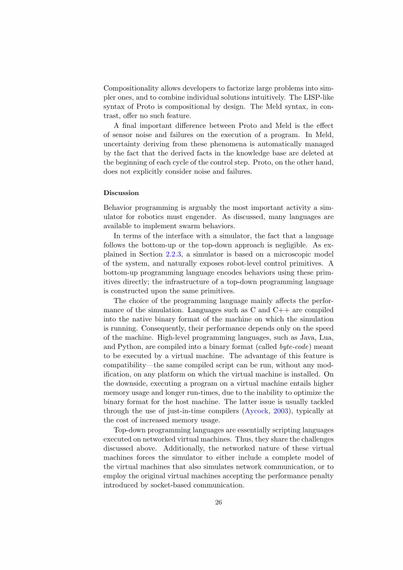
Compositionality allows developers to factorize large problems into sim-pler ones, and to combine individual solutions intuitively. The LISP-likesyntax of Proto is compositional by design. The Meld syntax, in con-trast, offer no such feature.

A final important difference between Proto and Meld is the effectof sensor noise and failures on the execution of a program. In Meld,uncertainty deriving from these phenomena is automatically managedby the fact that the derived facts in the knowledge base are deleted atthe beginning of each cycle of the control step. Proto, on the other hand,does not explicitly consider noise and failures.

Discussion

Behavior programming is arguably the most important activity a sim-ulator for robotics must engender. As discussed, many languages areavailable to implement swarm behaviors.

In terms of the interface with a simulator, the fact that a languagefollows the bottom-up or the top-down approach is negligible. As ex-plained in Section 2.2.3, a simulator is based on a microscopic modelof the system, and naturally exposes robot-level control primitives. Abottom-up programming language encodes behaviors using these prim-itives directly; the infrastructure of a top-down programming languageis constructed upon the same primitives.

The choice of the programming language mainly affects the perfor-mance of the simulation. Languages such as C and C++ are compiledinto the native binary format of the machine on which the simulationis running. Consequently, their performance depends only on the speedof the machine. High-level programming languages, such as Java, Lua,and Python, are compiled into a binary format (called byte-code) meantto be executed by a virtual machine. The advantage of this feature iscompatibility—the same compiled script can be run, without any mod-ification, on any platform on which the virtual machine is installed. Onthe downside, executing a program on a virtual machine entails highermemory usage and longer run-times, due to the inability to optimize thebinary format for the host machine. The latter issue is usually tackledthrough the use of just-in-time compilers (Aycock, 2003), typically atthe cost of increased memory usage.

Top-down programming languages are essentially scripting languagesexecuted on networked virtual machines. Thus, they share the challengesdiscussed above. Additionally, the networked nature of these virtualmachines forces the simulator to either include a complete model ofthe virtual machines that also simulates network communication, or toemploy the original virtual machines accepting the performance penaltyintroduced by socket-based communication.

26

2.2 Simulation of Swarm Robotics Systems

Real-robot experimentation is difficult due to the unreliability of today’srobotic hardware (Cao et al., 1997). As the number of robots involved inan experiment grows, maintaining the swarm in working condition be-comes prohibitive (Carlson et al., 2004). Thus, to date, the only methodto design and test for scalability is to employ modeling techniques, andvalidate the results with targeted real-robot experiments.

In this section, I present an overview of the techniques to modelrobot swarms. In Section 2.2.1, I provide a general view of the modelingtechniques. In Section 2.2.2, I focus on physics-based approaches.

2.2.1 Modeling Robot Swarms

The literature abounds in modeling approaches that differ widely inpurpose and level of abstraction.

Regarding their purpose, modeling techniques can be qualified withrespect to their role in the development life cycle. A non-executablemodel typically describes the required properties of the system prior toits implementation. Executable models, on the other hand, reproducethe dynamics of the running system. To date, due to the difficulty ofpredicting swarm behaviors, non-executable models have received lit-tle attention in the literature. Two notable exceptions exist: Winfieldet al. (2005), who apply temporal logic to model self-organization; andBrambilla et al. (2012), who propose a multi-level approach to swarmdesign based on formal methods. The vast majority of work in swarmmodeling, however, focuses on executable models.

Furthermore, based on the level of abstraction, we can divide modelsin three families: macroscopic, microscopic, and mesoscopic.

Macroscopic models represent the system from the global point ofview, as a single entity. Many modeling techniques in this family areinspired by chemistry or physics (e.g., thermodynamics and synerget-ics). These models best capture behaviors such as flocking, aggregation,and diffusion, in which individuals can be represented as gas particles.However, these techniques are not suitable for describing behaviors inwhich individuals are more complex than randomly walking particles.In most complex swarm behaviors, aspects such as the robot body, itscapabilities, and the logic of its decision-making play a fundamentalrole (Hamann and Schmickl, 2012).

Microscopic models lay at the opposite end of the spectrum, as theyconsider the properties of each robot individually. Agent-based modelsinspired from biology fall in this category. However, the applicability ofthese models to swarm robotics is limited because natural and artificialsystems differ in two critical aspects. First, a given swarm behaviorcan be the result of a variety of individual behaviors (Edelstein-Keshet,

27

2001); second, robots and animals differ widely in terms of capabili-ties (e.g., sensing, locomotion) and communication means. As a con-sequence, models that explain natural behaviors might be extremelysuboptimal, or even not applicable to swarm robotics applications. Analternative approach to microscopic modeling based on control theoryhas been proposed by Gazi and Passino (2003). This approach, whileallowing one to prove the stability of a swarm behavior, assumes fullsynchronization, global communication, and absence of uncertainty.

Mesoscopic models place their focus between the two previous cate-gories by including both micro- and macroscopic elements, thus linkingmacroscopic phenomena to microscopic events. In the works of Marti-noli et al. (2004); Lerman et al. (2005); Correll and Martinoli (2006),the swarm is modeled considering the fraction of robots in a certainstate. The time evolution of these fractions is expressed through rateequations. While this method is relatively general and mathematicallytractable, it neglects the spatial aspects of a swarm. To overcome thisissue, Hamann and Worn (2008) proposed a modeling approach basedon Brownian motion.

2.2.2 Physics-Based Robot Modeling

The ultimate goal of a swarm model is to shed light on the relationshipbetween the macroscopic properties of the swarm and the microscopicinteractions of the individuals. To achieve this, the model must beexpressed at the suitable abstraction level, and allow for analytical in-vestigations. Despite the effort of the research community in the lastdecade, and the relatively large number of different approaches avail-able, to date, a commonly accepted ‘theory’ of swarm systems remainsunarticulated (Schweitzer, 2003). Moreover, the heterogeneity of theavailable approaches is an obstacle to the adoption of diverse methods,due to the steep learning curve of each.

To date, physics-based simulation remains the main technique to de-sign, prototype, and test swarm robotics systems. Physics-based modelsrely on minimal assumptions about the system, which can be summa-rized as ‘the robots possess a body.’ Additionally, physics-based model-ing is very general, as it targets a necessary feature of swarm systems—motion.

Modeling Motion

There exist several ways to model the motion of a robot (Gazi and Fidan,2007). In this section, I present four of the most employed models.

Kinematic Model. The simplest possible model to capture the motionof a robot in space is the kinematic model. In this model, the position

28

p of a robot follows the lawp = u,

where u is the control parameter. A robot modeled according to this lawbehaves like a mass-less particle capable of changing direction instanta-neously. Because of its low computational cost, this model is employedfor motion planning and for proof-of-concept navigation experiments.Additionally, this model is frequently used to study approaches to pat-tern formation and flocking inspired by virtual physics.

Point-Mass Model. The point-mass model is an extension of the kine-matic model in which the robot is represented as a geometrical point ofmass m. The motion of the robot follows the law:{

p = vmv = u + f ,

where p is the position of robot, v its speed, u is the control parameter,and f represents the effect of external forces, such as gravity. This modelis used for higher-precision simulations in the same situations in whichthe kinematic model proves useful.

Differential Steering Model. The differential steering model capturesthe motion dynamics of a two-wheeled robot. The robot state is [px, py, θ],where px, py indicate the position and θ the orientation of the robot.Denoting with ur and ul the right and left linear wheel speeds set bythe control system, and with b the inter-wheel distance, the model is:

px =ur + ul

2cos θ,

py =ur + ul

2sin θ,

θ =ur − ul

b.

This model is widely used to capture the motion of non-holonomicrobots. In addition, a robot can use it to perform dead reckoning fromodometry information.

Fully Actuated Model. The most complete model of robot motion isthe fully actuated model. This model captures the complete dynamicsof a robot composed of connected rigid bodies under the effect of variousforces. The model is:

M(q)q + f(q, q) = u,

where q ∈ Rn is the robot state (e.g., q = [p,v]), u is the control param-eter, M(q) is the inertia matrix, and f(q, q) is a function that accounts

29

for various effects such as: centripetal and Coriolis forces deriving fromrobot motion, external forces due to gravity and collisions, and randomdisturbances. This model captures the dynamics of mechanically com-plex and modular robots, in which multiple bodies are connected byjoints. Often, the term f(q, q) is expressed as a sum of two terms:

f(q, q) = fk(q, q) + fu(q, q),

in which fk(q, q) represents known forces, and fu(q, q) represents un-known disturbance. The inclusion of the unknown disturbance is em-ployed to develop algorithms that provide robustness to noise and/orperturbations.

Software for Physics Simulation

Several software packages for physics simulation (i.e., physics engines)are available. In their simplest form, these packages enable the simula-tion of the motion of a body in the space. Additionally, many physics en-gines include functionality such as collision detection and management,and provide means to interact with the internal spatial data structureand implement custom space-aware algorithms. Often, these softwarepackages constitute the core component around which robot simulatorsare built. In this section, I present the most significant physics enginescurrently available. All of these physics engines are based on the fullyactuated model.

Chipmunk Physics. Chipmunk Physics11 is a fast 2D physics enginewritten in C. It is designed to offer high performance for gaming and sci-entific applications. Chipmunk supports rigid bodies, and spatial datais organized into a space hash (Teschner et al., 2003). For this rea-son, Chipmunk excels at simulating hundreds of objects of similar size.To maintain high performance, Chipmunk internally uses an Euler in-tegrator. The basic version of Chipmunk is free and open source, andan enhanced version is available for a fee. In addition to the C inter-face, Chipmunk offers an API in Objective C and can be employed as aplug-in for the Unity Game Engine12.

Box2D. Box2D13 is a free and open source physics engine designed toperform fast simulations of rigid bodies. Similar to Chipmunk, Box2Demploys an Euler integrator. However, differently from Chipmunk, inBox2D objects are stored into a dynamic AABB tree (Zachmann, 2002).This structure is essentially a binary tree optimized to provide best

11http://chipmunk-physics.net/12http://unity3d.com/13http://box2d.org/

30

performance when the size of the simulated objects is heterogeneous.Box2D is written in C++, and offers an API in Objective C.

Open Dynamics Engine. Open Dynamics Engine (ODE)14 is a 3Dphysics engine that targets the simulation of rigid bodies. Over the lastdecade, ODE has been used for both gaming and scientific applications.In comparison to modern physics engines, the scalability of ODE forincreasing numbers of connected objects is known to be poor. ODEoffers two integration methods, a fast but unstable Euler integrator, anda slower but more stable fourth-order Runge-Kutta integrator. ODE wasoriginally written in C, but recently a C++ API has been added by thedeveloper community.

Bullet. Bullet15 is a state-of-the-art 3D physics engine capable of sim-ulating both rigid and soft bodies (cloth, ropes, deformable objects).Internally, spatial data is organized into a dynamic AABB tree (Zach-mann, 2002). Bullet can handle a large number of objects through CPUmulti-threading and its experimental GPU interface. Bullet offers bothEuler and Runge-Kutta integrators. Since its inception, Bullet has en-joyed increasing success and is now employed in a wide variety of soft-ware for gaming, visual effects for cinema, and scientific simulations.It is free and open source software, written in C++. Bullet can inter-operate with a large number of software packages such as Unity GameEngine16, Autodesk Maya16, and Blender17.

NVIDIA PhysX. NVIDIA PhysX18 is another state-of-the-art 3D physicsengine capable of a wide variety of simulations, including rigid and softbody dynamics, vehicle dynamics, volumetric fluid simulation, and clothsimulation. PhysX can handle a very large number of objects through itsnative support for multi-threading both on CPU and GPU, and integra-tion with NVIDIA Physics Processing Unit (PPU). PhysX is proprietarysoftware distributed with a free-to-use license for educational purposes.NVIDIA PhysX finds applications in gaming, CAD, visual effects forcinema, and scientific simulations. It offers a C++ interface and it isincluded in software packages such as Unity Game Engine8, AutodeskMaya20, Unreal Engine19, and Microsoft Robotics Studio20.

14http://ode-wiki.org/wiki/index.php?title=Main Page15http://www.bulletphysics.org/16http://www.autodesk.com/maya17http://www.blender.org/18https://developer.nvidia.com/physx19Since version 3, http://www.unrealengine.com/20http://www.microsoft.com/robotics/

31

Vortex. Vortex21 is a commercial 3D physics engine designed to sim-ulate complex multi-body simulations and robotics manipulation withhigh fidelity. It includes rigid body dynamics and a particle engine. Vor-tex is written in C++ and offers a wide variety of plug-ins to simulatesensing, grasping, and vehicle dynamics. Vortex has been employed in alarge number of applications in the military sector, as well as in gamingand scientific simulations.

Newton Game Dynamics. Newton Game Dynamics22 is a 3D physicsengine that simulates rigid body dynamics. Newton Game Dynamicssets itself apart from its competitors due to its deterministic collisionsolver, that yields truly reproducible simulations. On the downside, theperformance of this engine is inferior to Bullet’s and PhysX’. A multi-threaded version of Newton Game Dynamics (for both CPU and GPUcomputation) is currently under development, and it promises signif-icantly higher performance. Newton Game Dynamics is open sourcesoftware written in C++. It has been used for gaming and scientificsimulations.

Physics Abstraction Layer. Physics Abstraction Layer23 (PAL) is aunified interface for the most widespread physics engines. Rather thandirectly providing low-level functionality to perform physics simulations,PAL allows developers to construct physics-based software abstractingthe details of the underlying engine. In this way, the underlying physicsengine can be changed without affecting the rest of the application.Currently, PAL supports the following physics engines: Box2D, Bullet,Newton Game Dynamics, Open Dynamics Engine, and NVIDIA PhysX.

2.2.3 Simulators for Robotics

In this section, I review a number of important multi-robot simulatorsand discuss their features with respect to flexibility and scalability. Irestrict my focus to mainstream simulators, i.e., those widely used by theresearch community, and to less known simulators whose designs relateto ARGoS’. For a broader, although dated, discussion of developmenttools for robotics applications, including but not limited to simulators,I suggest the survey of Kramer and Scheutz (2006).

Simulators Targeting Flexibility

The design of general and flexible simulators is a relatively recent achieve-ment. Before the 2000s, CPU speed and RAM size on an average per-

21http://www.vxsim.com/en/software/why vortex/index.php22http://newtondynamics.com/forum/newton.php23http://pal.sf.net/

32

sonal computer were insufficient to support extensible designs while en-suring acceptable simulation performance. In the last decade, a fewsimulators able to support different types of robots were developed.

Gazebo. Gazebo24 (Koenig and Howard, 2004) is currently one of themost successful simulators in robotics. It is designed as a general toolfor a wide spectrum of applications. Gazebo allows users to define virtu-ally any kind of robot or environment through an XML-based simulationdescription format. This description is subsequently translated into low-level configuration for the physics engines and the other modules. Atthe time of writing, Gazebo offers two physics engines, ODE and Bul-let. The architecture of Gazebo is a publish-subscribe system formed byfour main processes, each dedicated to a specific task: physics simula-tion, sensor simulation, graphical visualization, and coordination of thesimulation loop. As a multi-process system, simulations in Gazebo pro-ceed in a parallel fashion. The primary benefits of a publish-subscribearchitecture lay in its high level of abstraction and generality, whichrender Gazebo very flexible. The physics process, for instance, exportsa message interface that can interoperate with the rest of the systemindependently of the specific choice of physics engine. Additionally, themessage-centric nature of this architecture lends itself to the creationof powerful analysis tools that act as consumers of the information ex-changed between the processes. The benefits of Gazebo’s architecturecome at the expense of efficiency, for two reasons. First, inter-processcommunication occurs through files and sockets, which are slow me-dia when the number of robots in a simulation increases. Second, theabstract message interface of Gazebo prevents the optimization of theaccess to the data structures that store the state of the simulated work.Gazebo is open source software written in C++. It is developed by theOpen Source Robotics Foundation25, which also maintains ROS. Thepublish-subscribe architecture of Gazebo is inspired by ROS and sharespart of the code-base. As a result, robot behaviors developed with ROScan be executed in Gazebo seamlessly.

Webots. Webots26 (Michel, 2004) is a commercial 3D simulator thattargets a wide variety of robotics applications. The Webots architectureis designed around the ODE physics engine. The environment and therobots are described in VRML, and are represented internally through atree structure. It is possible to interface directly to the underlying ODEstate, thus retrieving data useful for sensing, actuation, and creationof user extensions. However, this interface is available only for licensed

24http://gazebosim.org25http://osrfoundation.org/26http://www.cyberbotics.com/

33

copies of the software, and its use requires knowledge of both ODE andWebots internals. The scalability of ODE is known to be poor whencompared to state-of-the-art physics engines such as Bullet and NVIDIAPhysX. The main limitation of ODE is the lack of multi-threading, whichseverely limits its performance. For this reason, Webots is not suitablefor large-scale simulations involving thousands of robots. Webots iscommercial software written in C++. It offers models for a large varietyof common robotic platforms. Robot behavior can be written in C,C++, Java, Python, Matlab, and URBI.

USARSim. USARSim27 (Carpin et al., 2007a) is a 3D simulator de-signed for generic robotics scenarios. Since its inception, USARSim hasenjoyed increasing usage, and it is now the chief simulation frameworkfor the RoboCup Urban Search-and-Rescue League.1 With respect toother simulators, the community supporting USARSim has devoted sig-nificant effort to the validation of the robot models (Carpin et al., 2007b;Balakirsky et al., 2009). USARSim is built on top of Unreal Engine28,a commercial game engine released by Epic Games29. Unreal Engineprovides state-of-the-art technology for both physics simulation and re-alistic rendering. The models for robots, sensors, and other simulatedobjects, as well as the map of the environment, are specified in the pro-prietary format of Unreal Engine. At run-time, USARSim interacts withthe Unreal Engine through a socket-based interface. This interface al-lows users to specify control code for the robots. USARSim also providesadvanced debugging and monitoring tools implemented as ‘Unreal spec-tators’. The network-based architecture of USARSim imposes limits onthe number of robots that can take part in a simulation. Consequently,USARSim is unfit for large-scale experiments involving thousands ofrobots. Additionally, the dependency on a commercial game engine ren-ders adopting and extending USARSim problematic. USARSim is opensource software written in C++. It supports a wide variety of robots,and offers mechanisms to simulate wireless communication. USARSimallows the user to specify robot behaviors through Gamebot (Kaminkaet al., 2002), MOAST (Balakirsky and Messina, 2006; Balakirsky et al.,2008), and Player (Gerkey et al., 2003).

MuroSimF. MuroSimF30 (Friedmann et al., 2008) is a general-purposesimulator for multi-robot scenarios involving any kind of robot. Themain novelty of MuroSimF is the possibility to model any aspect of arobot with adjustable levels of accuracy. To obtain this feature, physics

27http://usarsim.sourceforge.net/28http://www.unrealengine.com/29http://www.epicgames.com/30http://www.dribblers.de/research/simulator.en.php?language=en

34

simulation in MuroSimF is not based on any mainstream physics en-gine. Instead, simulated objects are structured into tree-like compounds.Each object is assigned a dedicated model for simulation. Objects canalso be linked to simulate arms and grippers. Objects can also be as-sociated to a dedicate controller, thus realizing behaviors whose logic isdistributed across the subsystems of a robot. Parallelism in MuroSimFis achieved by submitting computation tasks (e.g., the update of anobject) to a scheduler, which distributes tasks across a pre-configuredthread pool. The architecture of MuroSimF allows the user to assigncomputational resources to those aspects of the simulation that are mostimportant for the current experiment. This feature is important, becauseit allows the user to avoid wasting computational resources on unimpor-tant aspects of the simulation. As a consequence, the performance ofMuroSimF is remarkable—experiments show that MuroSimF can sim-ulate dozens of robots in real-time with a simulation step as short as1/1000th of a second. The performance of MuroSimF is currently lim-ited by the fact that only part of the computation can be parallelized.In particular, collision detection and handling in MuroSimF are still ex-ecuted in a single thread. MuroSimF is open source software written inC++.

OpenRave. OpenRave31 (Diankov, 2010) is a simulator designed tosupport prototyping of motion planning and manipulation behaviors inindustrial applications. The architecture of OpenRave is organized infour components, internally called layers: (i) the ‘core’ layer acts as acoordinator of the activities of the other layers; (ii) the ‘plug-in’ layerdefines the basic interfaces for the modules executed in a simulation;(iii) the ‘scripting’ layer offers the means to specify the robot behaviors;and (iv) the ‘robot database’ layer provides a set of functions for theanalysis of robot behaviors based on metrics collected at run-time. Theexecution of a simulation is distributed across multiple threads. Onethread is dedicated to managing the environment, including physics andsensor calculations. The other threads execute the control logic. Thisdesign choice presents both advantages and disadvantages. The mainadvantage is the clear separation between environment simulation andcontrol logic. As mentioned, the target use case of OpenRave is motionplanning and manipulation for complex industrial applications. Thus,the control logic is likely to entail calculations whose computational costmight be comparable with the simulation of the environment. On thedownside, in this design the environment is a shared resource amongmultiple threads. Consequently, to prevent race conditions and ensureexclusive access to each thread, the entire environment must be locked

31http://www.openrave.org/

35

through a mutex. The assumptions upon which OpenRave’s design isconstructed are not true for swarm robotics. In swarm robotics, thecontrol logic typically has a negligible computational cost with respectto the simulation of the environment. In addition, it is not acceptablefor each access to the environment to be exclusive, as this prevents thecomputation to exploit parallelism efficiently. OpenRave is open sourcesoftware written in C++. It is integrated with Player, and allows devel-opers to specify robot behaviors in ROS, Python, and Octave/Matlab.

Morse. Morse32 (Echeverria et al., 2011) is a simulator designed forgeneral robotics scenarios. It is constructed around the Blender gameengine33, an extension of the Blender 3D rendering software that en-ables the creation of interactive animations with high-quality graphics.To simulate physics, the Blender game engine uses Bullet. The archi-tecture of Morse is multi-process. Morse allows the user to factorize thecomputation across processes, assigning a subset of the robots to eachof them. In this way, a complex simulation can be executed on a com-puting cluster, accelerating its execution. The processes are organizedinto a centralized system, in which a server node coordinates the workof the clients. The performance limitations of a multi-process architec-ture discussed for Gazebo also apply in the case of Morse. Additionally,the simulator is extended through Python scripts, imposing an abstrac-tion layer over C++ that further affects performance. Consequently,this design is not suitable for large-scale multi-robot scenarios. Simi-larly to its competitors, Morse is open source software written in C++.Additionally to the Python scripting interface, Morse allows the userto specify behaviors through popular middleware for robotics such asROS and YARP, and exposes a socket-based interface to enable furtherthird-party bindings.

SwarmSimX. SwarmSimX34 (Lachele et al., 2012) is a 3D simula-tor designed for real-time robotics applications, such as hardware- andhuman-in-the-loop scenarios. The main distinctive trait of SwarmSimXis the fact that the simulation loop is synchronized with wall-clock-timeto enable a realistic interactive simulation. SwarmSimX is built aroundNVIDIA PhysX, although the architecture permits the addition of newphysics engines. The architecture of SwarmSimX is extremely generic,as it revolves around three high-level concepts: visual representation,physical representation, and behavioral logic. The visual and physi-cal representations are independently specified. Both representationsare structured as trees. The visual representation has the purpose of

32http://www.openrobots.org/wiki/morse/33http://wiki.blender.org/index.php/Doc:2.6/Manual/Game Engine34https://svn.kyb.mpg.de/kyb-robotics

36

rendering a simulated object; the physical representation simulates itsdynamics. The behavioral logic is divided into ‘drivers’ and ‘sensors’.Drivers represent the behavior of a simulated object, while sensors pro-vide drivers with information on the simulated environment. A simu-lated object is represented through the concept of ‘artifact’, which is acomposition of visual/physical representation and behavioral logic. Thearchitecture of SwarmSimX achieves parallelism by assigning a dedi-cated thread to each artifact. Among the general-purpose simulators,SwarmSimX offers the best performance for multi-robot scenarios. Ex-periments in (Lachele et al., 2012) show that SwarmSimX is capable ofreaching real-time performance in a simulation with hundreds of quad-rotors. SwarmSimX is open source software written in C++. Behaviorscan be specified through ROS. In addition, SwarmSimX is integratedwith the TeleKyb framework (Lachele et al., 2013) for quad-rotor con-trol.

ReMod3D. ReMod3D35 (Collins et al., 2013) is a 3D simulator con-ceived for self-reconfigurable robotics. The main purpose of this softwareis to support the design of both physical and behavioral aspects of mod-ular robots. The architecture of ReMod3D is composed of a core modulethat manages a set of working modules. The working modules are ca-pable of connecting to each other in arbitrary topologies that can bemodified at run-time. A notable aspect of the design of ReMod3D is thepresence of explicit mechanisms for inter-module communication. Theflexibility of this design mainly revolves around the use of the genericC++ container Boost::any36. This container is used to handle modules,and to envelope exchanged messages across modules. The performanceof ReMod3D is remarkable. Experiments show that ReMod3D is capa-ble of simulating hundreds of modules in real-time. This performanceis primarily due to the GPU acceleration of the NVIDIA PhysX engineemployed to simulate the physics of the modules. However, reachingthousands of simulated modules in real time under the same experimen-tal conditions seems problematic with this design, due to the central roleof Boost::any. In fact, the generality of this container comes at thecost of forcing the system to perform a large number time-consumingtype conversions. ReMod3D is open source software written in C++.To the best of my knowledge, the authors do not provide any integrationwith third-party software.

V-Rep. V-REP37 (Rohmer et al., 2013) is among the most flexibleand feature-rich simulators available. V-REP targets a wide variety of

35http://www.isi.edu/robots/remod3d/36http://www.boost.org/doc/libs/1 55 0/doc/html/any.html37http://www.coppeliarobotics.com/

37

robotics applications, including navigation, motion planning, and ma-nipulation. The architecture of V-REP is complex and very general.Essentially, the architecture is a composition of modules with specificpurposes. Modules perform activities such as physics simulation (cur-rently through Bullet, ODE, or Vortex), sensor data retrieval, and robotcontrol. Modules can be freely added by the user. With respect to theprocess executing the main simulation loop, a module can be executedin three ways: (i) as a different process; (ii) in a dedicated thread; or(iii) on the same machine and thread. The core of the architecture ex-ports a Lua scripting interface, which is the primary mean to implementmodules in V-REP. Modules can be implemented also in C, C++, Java,Python, and URBI. The main strength of V-REP is its large collectionof extension libraries. V-REP is equipped with libraries for inverse/-forward kinematics, particle simulation, vision, and path planning. Themain limitation of V-REP is its high level of abstraction, which, similarlyto other designs analyzed in this section, prevents low-level optimization.V-REP is capable of executing multi-robot simulations, but to the bestof my knowledge performance evaluation has not been released. V-REPis written in C++ and it has been recently open sourced for academicuse. Its general architecture enables integration with any third-partyframework for robot control. Among the many, V-REP offers a ROSnode that interfaces with the ROS publish/subscribe network.

Simulators Targeting Efficiency

Stage. Stage38 (Vaughan, 2008) is a simulator designed to execute nav-igation experiments involving large groups of robots. The architectureof Stage revolves around a custom-made, 2D physics engine that mod-els robots through the kinematic and the differential steering models.The physics engine is capable of detecting collisions and perform basicray-cast queries. The shape of the simulated objects is represented asa collection of convex polygons, spatially indexed in a grid to improveperformance. Multi-threading is implemented by spawning one workerthread per CPU core. A master thread maintains a list of computa-tional tasks to perform and distributes the tasks to the worker threads.Stage’s performance is excellent in navigation-based experiments. Ex-perimental evaluation shows that Stage can simulate thousands of robotsin real-time. The underlying disadvantage of Stage is the simplicity ofits architecture, which renders it impossible to extend the simulator toperform more complex experiments. For instance, the kinematic natureof the models employed in Stage excludes the possibility to simulateself-assembly and foraging experiments. Another limitation of Stage isthe lack of noise in sensors and actuators. Stage is open source software

38https://github.com/rtv/Stage

38

written in C++. It is part of the Player project, and behaviors can bewritten both through Player and ROS.

Roborobo! Roborobo!39 (Bredeche et al., 2013) is a simple 2D simula-tor conceived for evolutionary experiments involving robot navigation.Similarly to Stage, Roborobo! is built around a custom-made physics en-gine. However, Roborobo!’s engine is simpler than Stage’s. The robotsare represented as particles, and motion simulation is limited to the kine-matic model. Collision detection exploits a slow pixel-based method,based on SDL’s getPixel32() function40. Roborobo!’s architecture issingle-threaded, and this severely limits its performance. Roborobo! isopen source software written in C++.

DPRSim and DPRSim2. The Claytronics project (Goldstein et al.,2009) aims to create a new kind of programmable matter formed by mil-lions of sub-millimeter robots. The technological difficulties to face inorder to reach this goal force the researchers in this project to prototypetheir solutions in simulation. However, the massively large-scale natureof the systems under study exceeds the capability of any known robotsimulator to offer acceptable performance. For these reasons, Ashley-Rollman et al. (2011) designed DPRSim, a software that simulates large-scale robot ensembles. DPRSim is based on a modified version of ODE,that is capable of multi-threaded computation with a reduced memoryfootprint with respect to the original implementation. These modifica-tions allowed Ashley-Rollman et al. (2011) to simulate ∼ 105 sphericalnanorobots in real time. To further improve performance and reach theobjective of ∼ 106 simulated robots in real time, Ashley-Rollman et al.(2011) designed DPRSim2, an improved version of DPRSim executed ona computing cluster. In DPRSim2, the simulated objects are distributedacross the computing nodes. The work of these nodes is coordinated bya dedicated master node, which maintains synchronization by issuing a‘tick’ signal that triggers an update across the other nodes. To improveperformance, the motion of the objects is not simulated; rather, objectsare ‘magically’ transported to their final destination at the due time.The impressive performance of DPRSim and DPRSim2 stems from de-sign choices tailored for a specific use case. As such, the design of thesesimulators is instructive but not generalizable. DPRSim and DPRSim2are open source software written in C++.

39https://code.google.com/p/roborobo/40http://www.libsdl.org/

39

2.2.4 Discussion

Marrying flexibility and efficiency while ensuring satisfactory levels ofaccuracy is a difficult problem.

The simulators designed for flexibility fulfill their purpose throughmodularity and abstraction. Modularity is an obvious design choice toachieve flexibility, and its combination with high-level abstraction gen-erates designs that can suit a wide set of robotics applications. However,an abstract and modular architecture forces the developers to work farfrom key low-level aspects, such as data structures and the related al-gorithms to handle them. In other words, in an abstract and modulararchitecture, the presence of layers of abstraction imposes static choicesexactly where users would want to make modifications.

Conversely, the simulators designed for speed avoid abstraction andmodularity, in favor of an approach that targets a limited set of usecases.

In addition to this trade-off between efficiency and flexibility, the ar-chitectures of the analyzed simulators are ultimately wrappers arounda physics engine. When the number of robots taking part in an exper-iment rises, the physics engine becomes an increasingly larger factor inthe performance of the simulation. Beyond a certain level of perfor-mance degradation, these designs offer no solution to restore acceptablelevels of performance in physics simulation.

Summary

The design of a general-purpose simulator for swarm robotics is influ-enced by several factors.

First, swarm robotics is a research field with a wide range of long-term applications. These applications, despite their diversity, share com-mon aspects: (i) the robots have a minuscule scale with respect to thesize of the environment; (ii) the swarms are likely to be heterogeneousin terms of capabilities and assigned roles; both (iii) the physical prop-erties of environments and robots, and (iv) the communication meansvary considerably across applications.

Second, a simulator must be able to capture the capabilities of therobots composing the swarm in terms of locomotion, communication,self-assembling, and sensing. The wealth of long-term applications isreflected by the abundance in robotic platforms targeted to specific sce-narios, pushing for general and flexible simulator designs. At the sametime, the large numbers involved in swarm systems necessitate efficientand minimal (i.e., robot-specific) models.

Third, a simulator must act as a platform that enables both the de-sign and the implementation of artificial swarm systems. Currently, the

40

most widespread approach is bottom-up, whereby the designer conceivesthe system as a collection of intercommunicating individuals. Physics-based simulation is a precious tool to make this approach possible, dueto the minimal and general assumptions upon which it is founded.

A large number of physics-based simulators exist in the literature.Those simulators that concentrate on flexibility typically offer modularand general architecture capable of simulating any kind of robot. How-ever, such generality and flexibility are obtained at the cost of efficiency,due to the high level of abstraction of the architectural structure andthe mechanisms involved. Other simulators concentrate on efficiency,thus enabling experiments with hundreds, thousands, or even millionsof robots. These simulators obtain these remarkable results by sacrific-ing flexibility and accuracy, in favor of simpler and faster robot models.

41

Chapter 3

The ARGoS Architecture

In this chapter, I present the architecture of ARGoS. In Section 3.1 Idiscuss the requirements a simulator for swarm robotics must satisfy.Subsequently, I dedicate one section to each design choice: modularity(Section 3.2), customizable indexing (Section 3.3), execution of multiplephysics engines (Section 3.4), and multi-threading (Section 3.5).

3.1 Requirements

The main requirement a simulator must meet is accuracy. Accuracy is afunction of the fidelity of the individual models used in an experiment.It is a measurable property, whose threshold of acceptability dependson the application. For this reason, it is not uncommon to consider thecreation of an application-specific simulator as an integral part of theexperimental activities. Ideally, a simulator should display perfect ac-curacy. However, this is an unrealistic expectation, either for practicallimitations in the computational aspects of the employed models (e.g.,memory limitations, insufficient precision in floating-point operations,etc.), or for the lack of suitable models (e.g., sensor noise). The limit-edness of accuracy with respect to the real phenomena under study isoften called reality gap. In robotics, the reality gap is a serious issuethat hinders the transfer of behaviors developed in simulation onto thereal platforms (Meeden, 1998).

The second requirement a simulator must satisfy is efficiency. Anal-ogously to accuracy, efficiency cannot be considered an inherent featureof a simulator. Rather, it is a measurable property whose acceptancethreshold is set by the user considering the available resources (e.g., time,computation power). It is possible to identify two types of efficiency:static efficiency and dynamic efficiency. Static efficiency corresponds tothe wise use of computational resources (e.g., time, memory, CPU cores)in a specific experimental setup. Dynamic efficiency refers to the degra-dation of performance due to progressive changes in the parameters of

43

Loo

pfu

nct

ions

Controller

Sensors Actuators

Entities

Simulated 3D Space

PhysicsEngines

Media Visualizations

Control Interface

Figure 3.1: The architecture of ARGoS. The white boxes correspond to user-definable plug-ins.

the experimental setup. In swarm robotics, the main parameter of inter-est in an experimental setup is the swarm size, and dynamic efficiencycoincides with the concept of scalability.

The third requirement considered in this thesis is flexibility. Differ-ently from accuracy and efficiency, flexibility is an inherent property ofa simulator design. Flexibility can be generally defined as the capabilityof a simulator design to encompass a wide set of use cases. In this thesis,a design is considered flexible if it is capable of supporting any kind ofrobot swarm (see Section 2.1.2) and it allows researchers to perform anykind of experiment of relevance in the field (see Section 2.1.1).

These three requirements are interdependent. Increasing accuracy of-ten forces researchers to employ models with higher computational cost,thus lowering efficiency. A highly flexible design, as discussed in Sec-tion 2.2.4, is based on abstractions that prevent the user from optimizinglow-level aspects such as data structures and associated algorithms. Asa result, efficiency is lowered. In addition, the impossibility to imple-ment algorithms might result in a limitation of the models a simulatorcan execute, leading to lower accuracy.

3.2 Modularity

In software design, it is common practice to decouple a complex archi-tecture into several interacting modules. As discussed in Section 2.2.3,flexible simulators typically allow the user to modify modules or add newimplementations of modules to customize and enhance the functionalityof the program. The advantage of modularizing the robot model lies inthe possibility to choose which modules to employ for an experiment.Different modules are characterized by different accuracy and computa-

44

tional costs. Thus, the choice of which modules to employ correspondsto the allocation of accuracy where the user deems it necessary. I referto the possibility to allocate accuracy as tunable accuracy.

Tunable accuracy is one of the cornerstones of ARGoS design, as itenhances both flexibility and efficiency. Regarding flexibility the usercan define which modules to use for each aspect of the simulation. Effi-ciency is boosted by the fact that computational resources are allocatedonly where necessary.

In Figure 3.1, I report a diagram of the ARGoS architecture. Thewhite boxes in the figure correspond to user-definable plug-ins. As il-lustrated, not only controllers, robot and device models can be selected,but also physics engines and visualizations. In the rest of this section, Idescribe the features of each plug-in type in depth.

3.2.1 The Simulated 3D Space

The simulated 3D space, depicted at the center of Figure 3.1, is a collec-tion of data structures that contains the complete state of the simulation.This state information includes the position and the orientation of eachobject such as obstacles or robots. The state of objects composed ofdifferent parts or equipped with special devices, such as sets of coloredLEDs, is also stored in this space.

The data is organized into basic items referred to as entities. ARGoSnatively offers several entity types, and the user can customize them oradd new ones if necessary. Each type of entity stores information abouta specific aspect of the simulation.

For instance, to store the complete state of a wheeled robot, a com-posable entity is used. Composable entities are logical containers thatare used to group other entities. Composable entities can be nested toform trees of arbitrary complexity. The controllable entity is a compo-nent that stores a reference to the user-defined control code and to therobot’s sensors and actuators. The embodied entity component storesthe position, orientation and 3D bounding box of the robot. The currentwheel speed is stored into the wheeled entity component. If the robot isequipped with colored LEDs, their state is stored in a component calledLED-equipped entity.

Entity types are organized in hierarchies. For instance, the embodiedentity is an extension of the simpler positional entity, which containsjust the position and orientation of an object, but not its boundingbox. These design choices (entity composition and extension) ensureflexibility, enhance code reuse and diminish information redundancy.

Entity types are indexed in efficient data structures optimized foraccess speed. In this way, the performance of the plug-ins that accessthe simulated 3D space is enhanced (see Section 3.3).

45

3.2.2 Sensors and Actuators

Sensors and actuators are plug-ins that access the state of the simulated3D space. Sensors are granted read-only access to the simulated 3Dspace, while actuators are allowed to modify it. As explained in Sec-tion 3.2.1, information about the simulation state is stored in a numberof specialized entities. Sensors and actuators are designed to only accessthe necessary entities. For instance, the calculations of a distance sensoronly need to access information about the embodied entities around arobot, and can ignore other entities. In the same way, a robot’s LEDactuator needs only to update the state of that robot’s LED-equippedentity.

Tightly linking sensors and actuators to entity components has threebenefits: (i) these plug-ins can be implemented targeting specific com-ponents instead of the complete robot, often resulting in general (ratherthan robot-specific) models; (ii) the robot components associated withsensors and actuators that are not used in an experiment do not need tobe updated, avoiding waste of computational resources; (iii) new robotscan be created faster and more reliably by incorporating existing com-ponents, ensuring that all the sensors/actuators depending on them willwork without modification. Effects (i) and (iii) improve flexibility, whileeffect (ii) enhances efficiency.

3.2.3 Physics Engines

As illustrated in Section 3.2.1, an embodied entity is a component thatstores the position and orientation of a physical object in the 3D space.The state of the embodied entities is updated by the physics engines.

As it is explained in Section 3.4, physics engines are assigned non-overlapping portions of the 3D space. At each time step, each physicsengine is responsible for the update of the embodied entities that occupyits assigned portion of space. This design choice makes it possible to runmultiple engines of different types in parallel during an experiment.

Physics engines operate on a custom representation of their assignedportion of the 3D space. For instance, the position (x, y, z) of an objectin the 3D space could be stored as (x′, y′) in a 2D engine. At eachtime step, the 2D physics engine performs calculations to update itsinternal representation (x′, y′) and then transforms it into the common3D space representation. This design choice enables one to optimizeeach physics engine’s internal representation of space for speed, memoryusage and/or accuracy. Currently, ARGoS is equipped with four kindsof physics engines, designed to accommodate the most general use cases:(i) a 3D-dynamics engine based on ODE, (ii) a 3D particle engine, (iii)a 2D-dynamics engine based on the open source physics engine library

46

Chipmunk,1 and (iv) a 2D-kinematics engine.

3.2.4 Media

Communication is a fundamental aspect in the simulation of swarm sys-tems. It is only through communication that a swarm can achieve coor-dination. In Section 2.1.2, I have listed the many forms communicationcan take within a swarm. Essentially, communication occurs as a spa-tially localized phenomenon, in that robots can exchange messages onlywithin a limited range. In addition, devices such as cameras and therange-and-bearing system introduce the requirement that informationexchange can occur only if the involved robots are in direct line-of-sight.In other words, communication in swarms does not only involve dataexchange, but it also includes spatial aspects such as positioning andocclusions.

For this reason, simulating localized communication efficiently is dif-ficult. To allow third-party extension developers to select the best optionfor each type of communication mean, ARGoS offers two main methodsto simulate communication.

The first method simply consists in realizing pairs of dedicated sen-sors/actuators associated with communication-specific entity types. Ev-ery time a robot emits data, the actuator sets the data in the associ-ated communication entity, and the sensors of other robots receive thesedata by scanning the space for nearby communication entities. Whilethis method is simple to implement, it is often inefficient. The maincauses of inefficiency are two. First, if robot R1 can communicate withrobot R2, it is often the case that the inverse is true as well — R2 cancommunicate with R1. This is the case, for instance, of the range-and-bearing system. The second cause of inefficiency is the low locality ofthe data structures involved in the simulation of communication (seealso Section 3.3). In fact, every time a robot scans its neighborhood forcommunication entities, the data structures that store the wanted enti-ties must be loaded in cache, used once, and discarded to make room forthe next scan. Optimizing memory access in this context is difficult, andit is likely to entail a significant increase in the architecture complexity.

To cope with these issues, the ARGoS architecture offers a specializedmodule type called medium. A medium can be considered as a ‘physicsengine’ for communication. A medium stores the information aboutcommunicating entities in optimized data structures, and, analogouslyto a physics engine, upon update it executes the necessary data transferamong communication-specific entities. Media are very general moduletypes, and they can be used to simulate any kind of communicationexchange. Currently, ARGoS offers two types of media: (i) the range-

1http://code.google.com/p/chipmunk-physics/

47

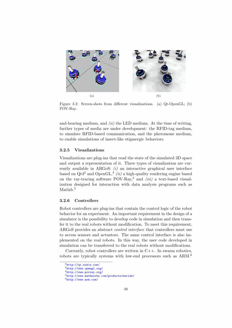
(a) (b)

Figure 3.2: Screen-shots from different visualizations. (a) Qt-OpenGL; (b)POV-Ray.

and-bearing medium, and (ii) the LED medium. At the time of writing,further types of media are under development: the RFID-tag medium,to simulate RFID-based communication, and the pheromone medium,to enable simulations of insect-like stigmergic behaviors.

3.2.5 Visualizations

Visualizations are plug-ins that read the state of the simulated 3D spaceand output a representation of it. Three types of visualization are cur-rently available in ARGoS: (i) an interactive graphical user interfacebased on Qt42 and OpenGL,3 (ii) a high-quality rendering engine basedon the ray-tracing software POV-Ray,4 and (iii) a text-based visual-ization designed for interaction with data analysis programs such asMatlab.5

3.2.6 Controllers

Robot controllers are plug-ins that contain the control logic of the robotbehavior for an experiment. An important requirement in the design of asimulator is the possibility to develop code in simulation and then trans-fer it to the real robots without modification. To meet this requirement,ARGoS provides an abstract control interface that controllers must useto access sensors and actuators. The same control interface is also im-plemented on the real robots. In this way, the user code developed insimulation can be transferred to the real robots without modifications.

Currently, robot controllers are written in C++. In swarm robotics,robots are typically systems with low-end processors such as ARM.6

2http://qt.nokia.com/3http://www.opengl.org/4http://www.povray.org/5http://www.mathworks.com/products/matlab/6http://www.arm.com/

48

Thus, transferring code from a personal computer to a real robot requiresrecompilation. Aside from the recompilation step, however, simulatedcode is directly usable on real robots.

I intend to integrate other programming languages that would notrequire recompilation to transfer code from simulation to real platforms.At the moment of writing, the ASEBA (Magnenat et al., 2010) and Luascripting languages have already been integrated in ARGoS, and furtherlanguage bindings (e.g., Python, PROTO) are under study.

3.2.7 Beyond Modularity: Loop Functions

It is very difficult to identify a set of features that can cover all the possi-ble use cases of multi-robot systems. Even though some features, such asrobot motion, are almost always necessary, many other features dependon the type of experiment considered. For instance, the metrics againstwhich statistics must be calculated depend on the experiment. Also, ifthe environment presents custom dynamics, such as objects being addedor removed as a result of the actions of the robots, these mechanismsneed to be implemented in the simulator. The need for specific andoften divergent features renders the design of a generic simulator ex-tremely complex. Furthermore, the approach of trying to add a myriadof features in the attempt to cover every possible use case usually ren-ders the learning curve of a tool much steeper, hindering usability andmaintainability.

To cope with these issues, I followed the common approach of pro-viding user-defined function hooks in strategic points of the simulationloop. In ARGoS, these hooks are called loop functions. The user cancustomize the initialization and the end of an experiment, and add cus-tom functionality executed before and/or after each simulation step. Itis also possible to define custom end conditions for an experiment.

Loop functions allow one to access and modify the entire simulation.In this way, the user can collect figures and statistics, and store complexdata for later analysis. It is also possible to interact with the simula-tion by moving, adding or removing entities in the environment, or bychanging their internal state.

Finally, loop functions can be used to prototype new features beforethey are promoted to the core ARGoS code.

3.2.8 Case Study: The Foot-bot and the Eye-bot

To discuss ARGoS modularity, I describe how two extremely differentrobots are modeled in ARGoS. The two robots I chose for this casestudy are the foot-bot (Bonani et al., 2010) and the eye-bot (Robertset al., 2007). The foot-bot is a ground-based robot that moves with a

49

Omnidirectionalcamera

Beacon

Range-and-bearingsystem

RGB-LED ring

Proximity + Lightsensor ring

RFID read/write

Ceiling/frontalcamera

Distancescanner

Gripper

Treels

Groundsensor

(a)

Ceiling attachment

Propellers

Range-and-bearingsystem

RGB-LED rings

Pan-and-tilt camera

(b)

Figure 3.3: (a) The foot-bot; (b) The eye-bot.

50

combination of wheels and tracks (called treels). The eye-bot is a quad-rotor aerial robot. Both robots are equipped with various sensors andactuators that allow them to interact with the surrounding environment.The robots and their devices are depicted in Figure 3.3.

Sensors and Actuators. Both robots are equipped with numerous sen-sors and actuators, and a few of them present similar features. In thefollowing discussion, I focus on the sensors and the actuators of the tworobots that share common aspects. It is important to note that somerobot devices may function both as a sensor and an actuator. In thesecases, in ARGoS two plug-ins are necessary—one for the sensor and onefor the actuator. One of the simplest devices present on both robots isthe on-board clock. The state of the clock is read by the clock sensor.Given its simplicity, ARGoS natively offers a single implementation ofthe clock sensor suitable for all the robots. Both the foot-bot and theeye-bot are equipped with LEDs. However, the specifics of the controlinterface of the LEDs are different, because the LEDs are distributeddifferently on the two robots. On the foot-bot, there are two kinds ofLEDs: a ring that surrounds the body, composed of 12 RGB LEDs,and a beacon positioned at the center of the robot body. The eye-bot isequipped with two rings of 16 LEDs each: an upper ring and a lower ring.The upper ring is primarily visible from the side, while the lower ring isvisible from beneath the robot. Although the control interface for theLEDs is different, the plug-ins share the same code base, thanks to theLED-equipped entity. Both the foot-bot and the eye-bot are equippedwith cameras. The foot-bot has two: an omnidirectional camera and acamera that can be mounted looking upwards or frontally. The eye-bothas a pan-and-tilt camera, that is, a camera mounted on a rotating de-vice. The implementation of the cameras is specific to each robot. Thecameras of the foot-bots are pure sensors, while the eye-bot’s pan-and-tilt camera has an associated actuator that controls the attitude of thecamera. Notwithstanding these differences, the implementations of thecamera sensors are based on a common definition that is extended tosuit the specific needs of each camera type, thus ensuring code reuse.

The foot-bot and the eye-bot can communicate with each other throughthe range-and-bearing communication device (Roberts et al., 2009), whichallows the robots in line-of-sight to exchange messages within a limitedrange. The particularity of this communication device is that a robot,upon receipt of a message, can calculate the relative position (distanceand angle) of the sender. The implementation of this device is dividedinto two parts: the range-and-bearing sensor and the range-and-bearingactuator. The role of the former is to manage the receipt of messagesfrom other robots. The role of the latter is to set the message to send.The implementation of this device is shared between the foot-bot and

51

the eye-bot.

Composing Entities. Both the foot-bot and the eye-bot are imple-mented as composable entities. They share most components. Bothare composed by an embodied entity, a controllable entity, and an LED-equipped entity. In addition, the state of the distance scanner is storedin a distance-scanner-equipped entity, while the state of the range-and-bearing communication system is stored into a range-and-bearing equippedentity. Both the LED-equipped entity and the range-and-bearing equippedentity are associated to their respective media, enabling communicationamong the robots. The cameras of the robots are represented by ded-icated camera-equipped entities. In particular, the foot-bot containsan omnidirectional-camera-equipped entity, while the eye-bot contains apan-and-tilt-camera-equipped entity. The foot-bot possesses a number ofentities that are not in common with the eye-bot, such as the ground-sensor-equipped entity, the light-sensor-equipped entity, the proximity-sensor-equipped entity, and the gripper-equipped entity. Data on motionactuation is stored into a wheeled entity for the foot-bot, and into apropeller-equipped entity for the eye-bot.

3.3 Entity Indexing

An important component of any physics-based robot simulation is howspatial data is handled. Spatial data structures are employed for all themost computationally intensive chores, such as collision detection, sens-ing, and communication. The choice of data structure heavily impactsthe performance of a simulator.

The main operations that must be performed over the spatial datastructure are insertion, deletion, update, and query. Insertion and dele-tion typically occur during the initialization and destruction phases ofa simulation, and affect performance only marginally. Update is usuallyexecuted once per loop. Query is the most frequent operation, being thebasis of the vast majority of the calculations for sensing and collisiondetection.

For this reason, in the choice of a data structure, priority is usuallygiven to the time complexity of the query operation. However, in allbut the most trivial cases, the time performance of a query depends onthe memory storage characteristics of the data structure. The memoryof a modern computer is organized into a multi-level hierarchy. Thetop-level memory, called L1 cache, is physically connected to the CPUand ensures the fastest access performance. This type of memory isexpensive and limited in size. Ideally, the necessary data to performa computation should not exceed the size of the L1 cache, and all thenecessary data should be present in this cache when needed. In practice,

52

however, maintaining the contents of this cache in optimal conditionsis a difficult problem. Whenever data is missing, (i.e., a cache missoccurs), the processor must wait for the data to be loaded from thelower-level cache, L2, losing precious time. Cache misses can occur atany level of the memory hierarchy, generating a cascade of load requeststhat eventually reach the main RAM storage. The time taken by aload request increases with the depth of such request in the hierarchy.Consequently, the time performance of a query operation on a spatialdata structure depends on the way the data is organized in memory. Inthis respect, an important desired property for a spatial data structureis locality, i.e., the capability to pack data in such a way to minimizethe number of cache misses.

The spatial data of a physics-based simulation is of two types: point-based data and object-based data (Samet, 2006). Point-based data con-sists of a vector x ∈ Rn, with n = 2 for two-dimensional simulationsand n = 3 of three-dimensional ones. This kind of data typically rep-resents the position of an object in the space. For simulations basedon the kinematic or point-mass models, point-based data is a commonrepresentation. Object-based data, on the other hand, is representedby an area or a volume in space. For instance, in collision detection,it is common to query the space to discover whether the body of anobject is intersecting another body. A common solution to this problemis wrapping every body of arbitrary shape with an axis-aligned bound-ing box, and calculate intersections among bounding boxes. For eachdetected bounding box intersection, the bodies therein are checked forintersection.

In ARGoS, spatial indexing is implemented as a policy (Alexan-drescu, 2001), and it can be used by any plug-in to index entities. Theability to specify the spatial indexing as part of the simulation setupis a unique feature of ARGoS with respect to existing designs. Thisfeature allows the user to fine-tune the performance of the simulation,thus increasing efficiency without affecting accuracy.

3.4 Multiple Physics Engines

The most distinctive feature of ARGoS is the possibility to partition thesimulated 3D space into non-overlapping portions of arbitrary size, andassign each portion to a different physics engine. For instance, in anenvironment formed by several rooms connected by corridors, the differ-ent rooms and the corridor could each be assigned a dedicated physicsengine. The volumes assigned to 3D engines are specified as right prismswhose size is user-defined, while the areas assigned to 2D engines arespecified as polygons in the 3D space. The user must define the effect ofa robot crossing the face of a prism (or the side of a polygon). There are

53

two kinds of faces (sides): walls and gates. Walls cannot be traversed—when a robot tries to cross a wall, the physics engine does not allow theaction. Conversely, when a robot traverses a gate, the robot is trans-ferred to another physics engine defined by the user in the experimentconfiguration file. This migration is performed automatically by ARGoSas robots navigate in the environment.

In practice, this partitioning is obtained by dividing the set of embod-ied entities in multiple subsets, and assigning each subset to a differentphysics engine. To avoid conflicts of responsibility among the physicsengines, I distinguish between mobile and non-mobile embodied entities.Mobile embodied entities are such that their state (position, orientation,3D bounding box) changes over time. Robots, as well as passive objectsthat can be pulled or pushed, fall into this category. Non-mobile embod-ied entities, on the other hand, never change state. Typical examples ofthis category are the structural elements of the experimental arena, suchas walls and columns. To ensure the correctness of the state of the sim-ulated space, I impose the condition that mobile embodied entities canbe managed by only one physics engine at a time. Non-mobile entities,instead, can be associated to as many engines as necessary. In this way,the structural elements of the arena are shared among all the engines,resulting in a consistent representation of the simulated 3D space.

When two robots are managed by different physics engines, they cannot interact physically (i.e., collide or grip each other). However, com-munication and sensing work across the physics engines. For example,ray casting is a typical method to simulate point-to-point communica-tion, occlusion checking and sensing. To check for ray intersections, asensor queries the simulated 3D space. The simulated 3D space con-structs a list of candidate embodied entities whose 3D bounding boxesintersect the ray. This step is very efficient because embodied entitiesare indexed in a space index (see Section 3.3). Next, each candidateembodied entity queries the physics engine in charge of its update toperform the actual ray-body intersection. The result is then returned tothe sensor that issued the check. Thus, even if the check is performedby a physics engine, the sensor does not need to interact directly withthe physics engine. This renders sensor development easy, because thereis no dependency between sensors and physics engines.

Because robots updated by different physics engines do not interactphysically, compenetrations are possible at the border between two en-gines. It is the user’s task to partition the space in such a way as to avoidthis phenomenon or to limit its impact on accuracy. A typical method,used, for example, in the experiments of Chapter 5, is to exploit the factthat robots can sense each other across physics engines and implementefficient obstacle avoidance strategies. Another solution is partitioningthe space appropriately. For example, in an experiment with flying and

54

1: Initialize2: Visualize the simulated 3D space3: while experiment is not finished do4: for all robots do5: Update sensor readings6: Execute control step7: end for8: for all robots do9: Update robot status

10: end for11: for all physics engines do12: Update physics13: end for14: Visualize the simulated 3D space15: end while16: Cleanup

} sense+control

} act

} physics

Figure 3.4: Simplified pseudo-code of the main simulation loop of ARGoS.Each ‘for all’ loop corresponds to a phase of the main simulation loop. Eachphase is parallelized as shown in Figure 3.5.

wheeled robots, flying robots could be assigned to one physics engine andwheeled robots to another. As long as the flying robots stay sufficientlyhigh, collisions with wheeled robots are not possible.

In Chapter 5 I empirically demonstrate that the use of multiplephysics engines results in a significant decrease in simulation time.

3.5 Multiple Threads

To maximize simulation speed, the ARGoS architecture is designed toexploit modern CPU architectures. In practice, this is obtained by paral-lelizing the main simulation loop reported in Figure 3.4. During the ex-ecution of the loop, sensors and visualizations read simulated 3D space,while actuators and physics engines modify it. Thus, simulated 3Dspace is a shared resource. In multi-threaded applications, simultaneousread/write access on shared resources requires careful design, as accessconflicts (race conditions) could potentially occur. A typical solution toprevent race conditions is to employ mutexes or semaphores. However,these solutions typically entail significant performance costs (Tanen-baum, 2001). Therefore, to improve performance, I designed the mainloop and the simulated 3D space in such a way as to avoid race condi-tions altogether. These design choices benefit not only performance: thelack of race conditions means that plug-ins do not need to synchronizeor manage resource access explicitly, thus simplifying their development.

55

s1

s2

..

.

sP

s1

s2

..

.

sP

s1

s2

..

.

sP

m m m m

main main main main

sense+control act physics

Figure 3.5: The multi-threading schema of ARGoS is scatter-gather. Themaster thread (denoted by ‘m’) coordinates the activity of the slave threads(denoted by ‘s’). The sense+control, act and physics phases are performed byP parallel threads. P is defined by the user.

The main simulation loop is composed of three phases executed in se-quence: sense+control, act and physics. In the first phase (sense+control,lines 4–7 of the algorithm in Figure 3.4), the robot sensors read the stateof the simulated 3D space. The robot controllers use such informationto execute the control step. At the end of this phase, the actions chosenby the robot controllers are stored into the actuators, but the actionshave not yet been executed. Therefore, this phase is read-only, and raceconditions are not possible. In the second phase, act (lines 8–10 of thealgorithm in Figure 3.4), the actions stored in the actuators are exe-cuted. All the component entities of each robot in the simulated 3Dspace are updated, with the exception of the embodied entities. Raceconditions cannot occur because, as explained in Section 3.2, each actu-ator is linked to a single robot component, and two actuators cannot belinked to the same component of a specific robot. In the third and finalphase, physics (lines 11–13 of the algorithm in Figure 3.4), the physicsengines update the state of the embodied entities. Race conditions arenot possible because, as explained in Section 3.4, in each simulation step,mobile embodied entities are associated to one and only one physics en-gine, and embodied entities in different physics engines do not interact.Furthermore, physics engines do not need synchronization, because theduration of the simulation step is set as a parameter in the experimentconfiguration file and is common to all the physics engines.

Each phase is executed by a set of P slave threads. This parameteris chosen by the user in the experiment configuration file. Experimentalevaluation demonstrates that maximum performance is reached whenP matches the number of available processor cores (see Chapter 5). Amaster thread coordinates the beginning and the end of each phase. InFigure 3.5 the master thread is indicated by ‘m’ and the slave threadsare indicated by ‘s’. Execution proceeds in a scatter-gather fashion.At the beginning of each phase, the slave threads are idle. When the

56

Robot1

Sensors

Actuators

Controller . . . RobotN

Sensors

Actuators

Controller

Global Space

(a) Sensor update and control step.

Robot1

Sensors

Actuators

Controller . . . RobotN

Sensors

Actuators

Controller

Global Space

(b) Robot state update, excluding physics-related information.

Entity1

Entity2

. . . EntityL− 1

EntityL

Global Space

PhysicsEngine 1

PhysicsEngine

M

(c) Update of the physics-related entity information.

Figure 3.6: Information flow in the various phases of the main simulation loopof ARGoS. The robot entities live in the global space. A controller and a setof sensors and actuators are associated to each robot. (a) In the initial phase,robot sensors collect information from the global space. Subsequently, robotcontrollers query the sensors and update the actuators with the chosen actionsto perform. (b) The chosen actions stored in the actuators are executed, thatis, the robot state is updated. At this point, positions and orientations havenot been updated yet. (c) The physics engines calculate new positions andorientations for the mobile entities under their responsibility. Collisions aresolved where necessary.

57

master thread sends the ‘start’ signal, the slave threads execute theirwork. Upon completion, the slave threads send the ‘finish’ signal to themaster thread and switch back to idle state. When all the slave threadsare done, the master thread sends the ‘start’ signal for the next phase.

The computation to be executed in each phase is decoupled in tasksassigned to the P slave threads. In the sense+control phase, a task isto update a robot’s sensors and then execute its controller. In the actphase, a task is to update a robot’s actuators. In the physics phase,a task is to update one physics engine. Two methods are available inARGoS to assign tasks to threads. The first method is to pre-computetask assignment at the beginning of the experiment, distributing thetasks evenly among the threads. The assignment is kept constant unlessrobots are added or removed during the experiment. This method givesthe best performance when the tasks performed by each thread havesimilar computational costs. This occurs, for instance, when all of therobots execute the same controller and the robots are evenly distributedacross the physics engines. Otherwise, the duration of each phase of theloop corresponds to the time spent by the slowest thread to perform itspart of the work. To solve this problem, a second method, called h-dispatch (Holmes et al., 2010), is available in ARGoS to assign tasks tothreads. In this method, an additional thread called dispatcher is used.The dispatcher manages the list of tasks to perform at each phase. Toperform a task, a thread receives it from the dispatcher. When the taskis completed, the thread requests a new task until all the tasks have beenperformed. Then, the master thread sends a signal to the dispatcher tomanage the tasks of the next phase, and the slave threads are awakenand resume fetching tasks. This method gives best performance whenthe tasks are very diverse. For example, if a slave thread happens toreceive a long task from the dispatcher, the other slave threads canperform multiple shorter tasks in the meantime. However, if the tasksare very similar to each other, this method proves to be slower thanpre-assignment, as the slave threads tend to finish at the same time andspend most of the time waiting for the dispatcher thread to assign newtasks to them. The choice of the thread assignment method is left tothe user as a parameter in the experiment configuration file.

The scheduling strategy in ARGoS is implemented as a policy, anal-ogously to spatial indexing. This design choice makes it possible to addnew scheduling strategies to ARGoS. This choice is conceived to enablefuture research in optimal task scheduling, possibly including strategiescapable of self-configuring depending on the type of experiment at hand.

58

Summary

In this chapter, I presented the ideas that underlie the design of ARGoS.From the discussion in Chapter 2, I derived a number of requirementsthat a successful design must respect: (i) accuracy, which is the degree ofcorrespondence between results obtained in simulation and in real-worldexperiments; (ii) efficiency, in the form of static efficiency (i.e., the wiseuse of computational resources) and dynamic efficiency (i.e., the capa-bility to maintain the simulation performance within acceptable boundsfor the parameter range in which experimentation is performed); and(iii) flexibility, cast as the possibility to execute any kind of experiment,given the appropriate models. While flexibility is an intrinsic propertyof a simulator design, accuracy and efficiency are extrinsic, because theydepend on the needs of the experimenter.

The first design choice to achieve the above requirements is modu-larity. Differently from the abstract, high-level nature of the simulatorarchitectures discussed in Chapter 2, the architecture of ARGoS is de-composed into modules that map directly to the aspects a user mightwant to override, namely entities, sensors, actuators, physics engines,media, controllers, and even visualizations. For added flexibility, AR-GoS offers a special kind of module, called ‘loop functions,’ that allowsthe user to interact with the simulation by injecting experiment-specificlogic to derive statistics, modify the course of an experiment, or insertnew functionality. Through the wise choice of modules, the user cantune the accuracy of the simulation, and at the same time enhance effi-ciency by assigning less computational resources to the aspects that donot influence its dynamics.

The second design choice of ARGoS stems from the fact that a largepart of the computational resources is dedicated to managing spatialdata. Many algorithms for spatial indexing exist, and their performancevaries depending on the characteristics of the objects to handle. For in-stance, array-based methods offer best performance when a large numberof similar objects is simulated; however, when the objects vary in size,tree-based methods tend to perform better. To ensure maximum per-formance, in ARGoS spatial indexes are cast as policies, and the usercan select the most appropriate in a case-by-case fashion.

The third design choice is the possibility to partition the physicalspace into multiple regions, assigning each region to a dedicated physicsengine. This feature of ARGoS distinguishes it among the existing sim-ulators. By employing multiple physics engines, the simulation is exe-cuted faster, because each engine must handle a lower number of entities.Additionally, each engine can be specialized for a scenario, such as un-derwater experiments or navigation on a shore. In this way, complexexperiments can be executed while, at the same time, maintaining the

59

right level of accuracy for each aspect and ensuring efficiency.The fourth design choice is multi-threading. In ARGoS, multi-threading

is realized by considering the update of each part of a robot as a sep-arate task. In this way, the granularity of the tasks is very thin, andparallelism is enhanced. The time taken by different tasks is typicallyvery diverse, creating the problem of properly scheduling the executionof the tasks. ARGoS currently offers two scheduling algorithms: thefirst is designed to efficiently schedule tasks whose duration is similar;the second is designed to provide best results when the task duration isheterogeneous. Task scheduling is implemented as a policy, thus makingroom for future improvements.

60

Chapter 4

Achieving Flexibility

In Chapter 3, I presented an abstract view of the structure of ARGoS.I highlighted the fact that the ARGoS architecture is organized into anumber of modules, each of which fulfills a specific purpose. From thearchitectural point of view, a user extension is essentially an instance ofa specific module. The extremely flexible nature of ARGoS primarilyderives from this design choice.

In this chapter, I present the approach adopted in ARGoS to realizethe architectural view of Chapter 3. In Section 4.1, I illustrate require-ments and desired features, arguing that realizing the ARGoS architec-ture is challenging. In Section 4.2, I focus on the basic aspects of thedesign of the ARGoS architecture. By “basic”, I mean those aspectsthat do not constitute a challenge. In Section 4.3, I move my atten-tion to the real design challenges, by (i) highlighting the shortcomingsof a number of common approaches, and (ii) presenting the approach Ifollowed in the design of the ARGoS architecture.

4.1 Requirements

Figure 4.1 reports a high-level representation of the required interactionsamong the ARGoS core, the developers of new modules, and the usersthat run simulations. As it can be inferred from the figure, realizing thearchitectural vision of Chapter 3 translates into designing mechanismsto achieve two purposes: (i) managing the available modules effectively,and (ii) separating the work of extension developers and end users. Thedesign of these mechanisms are challenging because they must meet anumber of diverse requirements that involve several aspects.

From the point of view of the design of the ARGoS core itself, tworequirements are paramount: independence and efficiency. Independencemeans that the addition of new modules must avoid any modification ofthe ARGoS core. In other words, the ARGoS core must not depend onany specific module—although the implementation of a module depends

61

developer 1

developer 2

module 1

module 2

develops

develops

operates on ARGoScore

register

into

registerinto

user

requests

list/help to

behavior/ loop

functions

register

into

.argos

file

develops

writes

configures

Figure 4.1: A high-level diagram representing the required interactions amongdevelopers, users, and the ARGoS core.

on the current version of the ARGoS core. Efficiency refers to theability of the core to manage the life cycle of the different modules withminimum computational overhead.

From the point of view of the developer of extensions, flexibility andtype safety are the main concerns. The different types of modules thatcompose the ARGoS architecture categorize the possible types of exten-sions ARGoS accepts. However, the actual logic contained in a moduleimplementation is completely unforeseeable by ARGoS. To respect therequirements of efficiency and tunable accuracy, the ARGoS architec-ture must prove flexible enough to allow for highly optimized imple-mentations of a certain module. In addition, often a certain moduleimplementation involves direct interactions with other modules. It isimportant to notice that also the type of interaction between modulesis unforeseeable by ARGoS, thus the core must provide a mechanismto enable arbitrary module-to-module interactions. For this kind of in-teractions to occur, besides flexibility ARGoS must ensure type safety,i.e., ARGoS must prevent incorrect interactions from happening. Forinstance, consider the interaction between entities and visualizations.Entities are added to the space, and the visualization has the task ofrepresenting the state of the space to the user, usually through graph-ics. To this aim, the visualization module must possess a specializedmodel for each type of entity, and display the right model accordinglyto the state of each actual entity. To obtain its state, the visualizationmust interface directly with the entity—for independence, the ARGoScore cannot possess specific information on an entity. In this example,type safety is ensured if ARGoS prevents a visualization from renderingan entity with the wrong model. Also, in case a model for a certainentity type is missing, ARGoS must provide mechanisms to inform theuser that the corresponding entities cannot be visualized. Without type

62

safety, extension development would be cumbersome and error-prone,forcing the developer to include error-checking routines that are likelyto lower the performance of an experiment run.

From the point of view of the user, simplicity is the key requirement.Operations such as choosing and loading a module should be performedwith minimal effort. To ease the choice of the most suitable modules, thesystem must construct, manage, and present a list of available modules,along with a detailed usage guide. In addition, it is desirable that themechanism to load experiment-specific logic (e.g., robot control code andloop functions) is analogous (or, preferably, identical) to the mechanismto load other modules, such as sensors and actuators.

Satisfying all of the above requirements is challenging. In the sub-sequent discussion, I divide the presentation of the final design in twoparts. In Section 4.2, I illustrate the basic mechanisms to store modulesand load them at the beginning of an experimental run. In Section 4.3,I criticize a number of classical techniques to enable arbitrary interac-tions among modules, highlighting their limitations with respect to therequirements above mentioned; subsequently, I explain the solution Iemployed to satisfy all the requirements.

4.2 Modules as Plug-ins

To satisfy the independence requirement, i.e., new extensions must notforce a change into the ARGoS core, modules are implemented as plug-ins. Plug-ins are the classical approach to enable third-party additionsto a software without modifying its architecture nor requiring recompi-lation (independence). Plug-ins are software libraries that can be linked(and unlinked) at any moment during the life-time of the target soft-ware. In modern computing, plug-ins constitute the backbone of manyprograms of widespread use. For instance, modern web browsers useplug-ins to visualize special content such as Flash videos; media play-ers encapsulate audio/video codecs into plug-ins; software developmentenvironments support additional programming languages through ex-tensions implemented as plug-ins.

In this section, I will sketch the design of the plug-in manager ofARGoS. In Section 4.2.1, I explain how the various plug-in types areorganized. In Section 4.2.2, I describe the actual plug-in manager.

4.2.1 The Plug-in Hierarchy

Regardless of its intended task, the life-time of a plug-in is usually com-posed of at least three phases: initialization, execution, and destruc-tion. Initialization consists in performing the necessary duties for theexecution to occur. Typically, configuration and memory allocation are

63

CBaseConfigurableResource

+Init(TConfigurationNode&):void

+Reset():void

+Destroy():void

CCI Controller

+Init(TConfigurationNode&):void

+ControlStep():void

+Reset():void

+Destroy():void

CLoopFunctions

+Init(TConfigurationNode&):void

+PreStep():void

+PostStep():void

+Reset():void

+Destroy():void

CCI Actuator

+Init(TConfigurationNode&):void

+Reset():void

+Destroy():void

CPhysicsEngine

+Init(TConfigurationNode&):void

+Update():void

+Reset():void

+Destroy():void

CCI Sensor

+Init(TConfigurationNode&):void

+Reset():void

+Destroy():void

CMedium

+Init(TConfigurationNode&):void

+PostSpaceInit():void

+Update():void

+Reset():void

+Destroy():void

CVisualization

+Init(TConfigurationNode&):void

+Execute():void

+Reset():void

+Destroy():void

CEntity

+Init(TConfigurationNode&):void

+Update():void

+Reset():void

+Destroy():void

Control InterfaceSimulator

Figure 4.2: A UML class diagram of the basic plug-in hierarchy in ARGoS.

64

performed during this phase. The execution phase contains the actuallogic of the plug-in. Destruction reverts the actions performed duringinitialization, such as disposing of memory and closing open files. InARGoS, beyond these phases, a fourth one is present—reset. The resetphase has the task of reverting the state of the simulation to what itwas right after initialization.

Figure 4.2 depicts a class diagram of the plug-in hierarchy of theARGoS core. The basic plug-in type is CBaseConfigurableResource,which contains three methods—Init(), Destroy(), and Reset(). Thesemethods execute the corresponding three phases in the plug-in life cycle.The fourth phase, execution, is not present in the base class. I madethis choice for two reasons.

First, because the execution logic of a plug-in is not always containedin one method. For instance, the execution logic of the CLoopFunctionsclass is split in two methods, PreStep() and PostStep(), executed rightbefore and right after a complete simulation update step has occurred.Also the CCI Sensor and CCI Actuator classes require special treat-ment. As depicted in Figure 3.1, the purpose of the control interface isto abstract away the fact that the underlying robot is simulated or real.The control interface, in fact, is composed of a set of interfaces that in-herit from the CCI Sensor and CCI Actuator classes. The “real” workis performed by suitable implementations of these classes. On the realrobot, a sensor’s job is to collect data from the robot; in a simulation, asensor’s job is to calculate the same data. Similarly, on the real robot,an actuator must use the platform primitives to execute the actions dic-tated by the control logic; in a simulation, an actuator must modify therobot state. On the real robot, the implementation of these classes de-pends on the internals of the robotic platform. Often, data between thecontrol interface and the robot subsystems is exchanged asynchronously,either through interrupts (e.g. the e-puck) or message passing (e.g., thefoot-bot). In this case, a single update method is useless. In the sim-ulator, on the other hand, data is managed synchronously, which callsfor an explicit update method.

The second reason for not having an explicit execution method in thebase plug-in class is that it is desirable, for readability purposes, thatthe name corresponding to the execution method is somehow related tothe kind of logic it is supposed to contain. For instance, ControlStep()is a good choice for the CCI Controller class, and Update() fits wellthe purposes of the CPhysicsEngine and CEntity classes.

4.2.2 Plug-in Management

In general, the plug-in manager is a software component that performstwo basic tasks: (i) allowing the system to create new instances of a

65

given plug-in when necessary; and (ii) registering new plug-in imple-mentations.

Regarding the creation of new plug-in instances, the classical ap-proach is to employ the Factory Method pattern (Gamma et al., 1994).This design pattern tackles the problem of creating an instance of a classwithout knowing its interface. The main idea is to provide an interfaceto create an object, and defer the actual operations to perform this taskto a type-specific implementation. Since in ARGoS many plug-in typesexist, I slightly generalized this pattern (see Section 4.2.3). As an addedbenefit in terms of independence and flexibility, the resulting systemcan be exploited by an extension developer or by the end user to createfurther plug-in types with only a couple of lines of code.

In order to register a new plug-in, the plug-in manager requires notonly its implementation, but also a certain quantity of metadata. In theEclipse IDE,1 for example, each plug-in is bundled with an XML filecalled manifest that contains the human-readable name of the plug-in,its version, details about the functionality it implements, as well as a linkto the actual plug-in binary. Upon initialization, the Eclipse core spansthe plug-in directories, opens each bundle, and retrieves the informationon every available plug-in. This system is effective and widespread inplug-in-based software. However, its main drawback is forcing the coreto open and parse a large number of text files upon initialization, whichresults in long start-up times when many plug-ins must be scanned. Toavoid this issue, for ARGoS I chose to include the metadata directly intothe plug-in binary. This approach, explained in Section 4.2.3, has thebenefit that the metadata is pre-parsed and automatically loaded intothe ARGoS core, making initialization and help queries extremely fast.

4.2.3 The Plug-in Factory

The class diagram of the plug-in manager is reported in Figure 4.3.The CFactory template is the core of the plug-in manager. Its in-

terface offers three methods—GetTypeMap(), Register(), and New(),to query the available plug-ins, register a new plug-in, and create aninstance of a specific plug-in, respectively. Internally, CFactory uses ahash map of STypeInfo structs to store the plug-in metadata and afunction pointer to the plug-in creator. In the hash map, each struct isassociated to a string label that identifies a specific plug-in implementa-tion. CFactory is a static class because, besides the hash map, it doesnot need to maintain any state information.

CFactory is a template whose parameter T corresponds to the baseof the plug-in hierarchy (e.g., CCI Controller, CPhysicsEngine, etc.),

1http://www.eclipse.org/

66

CFactory

+GetTypeMap():TTypeMap&

+Register(...):void

+New(string& label):void

T=PluginBase

<<struct>>

CFactory::STypeInfo

+Creator:TCreator*

+Author:string

+Version:string

+BriefDescription:string

+LongDescription:string

+Status:string

T=PluginBase

string

1

<<function pointer>>

TCreator:(T*)(*)()

T* U ## Creator {return new U;

}

T=PluginBase

U=MyPlugin

1

Maps the plug-in labelto its metadata

PluginBase

C ## U ## Proxy

+C ## U ## Proxy() {CFactory<T>::

Register(..., U ## Creator);

}

T=PluginBase

U=MyPlugin

calls

uses

MyPlugin

+MyPlugin()

uses

Figure 4.3: A UML class diagram of the ARGoS plug-in manager. In thisdiagram, I use the notation A ## B to express the string concatenation operatorof the C++ pre-processor. In the C++ pre-processor, the expansion of asymbol X corresponds to its definition, if the symbol was previously defined;otherwise its expansion corresponds to the symbol itself. Thus, A ## B is thestring resulting from the concatenation of the expansions of A and B.

indicated in the diagram as PluginBase . The choice of using a tem-plate class is a generalization of the classical Factory Method pattern.In the latter, CFactory is a class rather than a template, because theFactory Method pattern is designed to create plug-ins from a single hi-erarchy whose base is known in advance. However, in ARGoS, severalplug-in types exist (see also Figure 4.2). If one were to follow the clas-sical pattern strictly, the interface of the CFactory class would have toinclude dedicated methods GetTypeMap(), Register(), and New() foreach plug-in type. Thus, whenever a new plug-in type is added to AR-GoS, the interface of CFactory would require modifications. By makingCFactory a template whose parameter is the base of the plug-in hier-archy, these modifications are not necessary, and CFactory can be usedto create plug-ins from multiple hierarchies whose bases are not knownin advance. The benefits in terms of independence and flexibility aresignificant—the plug-in manager can even be used by extension devel-

67

opers and end-users to add custom plug-in types independently from theARGoS core.

Plug-in Creation

The creation of a plug-in instance occurs through the CFactory<T>::New()method.

This method accepts as a parameter the identifying label of thewanted plug-in implementation. Using this label, the method searchesin the hash map for the corresponding CFactory::STypeInfo struct.

The latter contains a function pointer (TCreator*) to the plug-increator function. As its name suggests, the role of the creator functionis to return a new instance of the wanted plug-in. For each type of plug-in, there exists a dedicated creator function, registered in the system asexplained in Section 4.2.3.

Plug-in Registration

The registration of a plug-in in ARGoS occurs through a mechanismcalled auto-registration. This mechanism exploits the way Unix-compatiblesystems link the global symbols of a library into an executable to piggy-back a call to CFactory<T>::Register().

The operation of linking a library into an executable is composedof a few phases. One of the earliest phases is the so-called static ini-tialization. During this phase, the linker collects information about theglobal symbols and, in particular, creates the global variables presentin the library. Normally, the creation of a global variable only impliesallocating memory. However, if the global variable is a class, it is alsopossible to include arbitrary code in its constructor.

The auto-registration mechanism consists in including a call to CFactory::Register() within the constructor of a suitably defined class declaredas global variable. The class is defined specifically for the plug-in im-plementation to register. In the class diagram of Figure 4.3, the plug-inimplementation class is MyPlugin. Thus, the registration class is namedCMyPluginProxy, which is the result of applying the ## operator to C## U ## Proxy when U is set to MyPlugin (see the figure caption for anexplanation on the ## operator).

In addition to the registration class, one must also define a plug-in-specific creator function. In Figure 4.3, the function is called MyPluginCreator,result of the operation U ## Creator.

The above actions are encapsulated into a macro called REGISTER SYMBOL.For the extension developer and the end user, registering a new plug-inimplementation is merely a matter of calling this macro.

68

Discussion

The registration of plug-in implementations and the creation of newinstances is a well-understood problem.

A slight generalization of the classical Factory Method pattern solvesthe problem of creating new plug-in instances, when multiple plug-inhierarchies exist whose base classes are not known in advance. Fromthe point of view of an extension developer, this solution guaranteesextreme flexibility; from the point of view of the ARGoS core design,the independence requirement is fully respected.

Registering new plug-in implementations is an equally simple prob-lem to solve, provided some knowledge of the internals of the Unix oper-ating system. The final result is a system that can register any plug-inusing the same underlying machinery. In addition, from the point ofview of the end user, the simplicity requirement is respected, becausethe internals of the registration logic are completely encapsulated in asingle macro definition.

4.3 Arbitrary Interactions among Modules

The requirement of allowing for arbitrary interactions among modulesmainly stems from the particular role that entities play with respect tothe other modules. In fact, entities store part of the state of a simulatedobject. Other modules, such as physics engines and visualizations, accessthe entities to perform their work—modifying the entity state or readingit. In other words, entities act as a mediator between other moduletypes. As discussed in Chapter 3, this design choice results in a clearfactorization of responsibilities among different modules, which, in turn,makes it possible to achieve multi-threading without introducing raceconditions.

4.3.1 Issues

A General View

The main issue in the realization of this design choice is that entities aremodules themselves, because developers must be given the possibility toadd new ones (e.g., robots or other objects) at will.

To better understand this issue, refer to Figure 4.1. In the figure, Ischematize the case in which two developers work separately. Developer1 implements module 1, and developer 2 implements a different module,module 2, which interacts with module 1. A third independent party,the user, downloads both modules and employs them in an experiment.For the sake of explanation, module 1 corresponds to a new robot, andmodule 2 corresponds to a new physics engine. Since I assume that thetwo developers work separately, developer 2 does not know in advance

69

CEntity CPhysicsEngine

+AddEntity(CEntity&):void

CMyEntity1

CMyPhysicsEngine

+AddEntity(CEntity&):void

CMyEntity2

add?

ARGoS core

Figure 4.4: A UML class diagram for an example problem of inter-modulecommunication. In this diagram, two entities must be added to a physicsengine. The entities and the physics engine are implemented by three differentdevelopers, out of the ARGoS core.

the features of the robot implemented by developer 1. Thus, the easiestsolution for developer 2 is to provide an API to create physics models forrobots, and leave the task of providing the models to other people. Con-versely, since an entity is supposed to be a mediator between modulescoded by several people, developer 1 must be able to define the featuresof the robot entity without having a specific module in mind. In otherwords, in this example, the problem is how to associate a physics modelfor a specific physics engine to a generic robot entity, when the two par-ties have been developed by different people. To make the picture evermore ambitious, the simplicity requirement dictates that these imple-mentation details are hidden from the user, who just wants to use themodules without knowledge of their internals; and the efficiency require-ment pushes towards a solution with minimal computational overhead.

It is easy to imagine that the machinery to realize arbitrary interac-tions between entities and other modules could be useful to enable otherinter-module interactions, too. A visualization, for instance, could in-terface directly with a specific sensor implementation to visualize extradata for debugging purposes.

Common Implementation Approaches

For the sake of explanation, in this section I will consider the interactionsbetween entities and physics engines, but the discussion is applicable toany kind of module. Figure 4.4 reports a UML diagram of the example.

70

In terms of classes, the problem of inter-module communication canbe expressed as follows. The ARGoS core maintains a number of datastructures, each dedicated to a specific module type. In particular, AR-GoS maintains a list of pointers to CEntity objects and a list of point-ers to CPhysicsEngine objects. Among the many interactions betweenthese two kinds of modules, consider the addition of an entity to aphysics engine. To achieve this, the physics engine must create an in-ternal representation of the entity body. Thus, the physics engine mustknow the exact type of the entity being added. However, the types ofboth the physics engine and the entity are defined outside the ARGoScore and known only at run-time. Consequently, the logic that addsa specific entity to a specific physics engine must be selected at run-time. In computer science, this problem is often referred to as dynamicdispatch (Lippman, 1996).

ARGoS is written in C++, because this language offers a good bal-ance between abstraction and performance. However, C++ has onlypartial support for dynamic dispatching—single dispatching.2 Singledispatching refers to the capability of the language to select the rightimplementation of a method based on the type of the class to which themethod belongs. This mechanism is one of the cornerstones of polymor-phism in C++. For the problem at hand, polymorphism (and, thus,single dispatching) is not sufficient. In essence, polymorphism refers tothe possibility to use a single interface for different objects, and to callthe right method implementations depending on the run-time type ofthe objects. In the example of Figure 4.4, this means that if the inter-face CPhysicsEngine exposes a public method AddEntity(CEntity&),and CMyPhysicsEngine implements AddEntity(CEntity&), then C++can select CMyPhysicsEngine::AddEntity(CEntity&) from a pointerto CPhysicsEngine. This mechanism does not achieve the completeresult because it is necessary to also dispatch over the argument ofthe CMyPhysicsEngine::AddEntity() method to select the right en-tity type. To work around this limitation of C++, several techniquesexist.

The Observer Pattern. In the Observer pattern (Gamma et al., 1994),an object, called the subject, maintains a list of other objects, called theobservers. Whenever its state changes, the subject notifies the observersof the fact. This pattern is often employed to implement event handlingmechanism, such as signal/slot. For the problem at hand, this pat-tern can be applied in two alternative ways. First, by equipping theCEntity class with a method for each possible operation a module canperform on it. This solution is not acceptable, because this would cre-

2Although an extension to support multiple dispatching has been proposed by Pirkelbaueret al. (2007)

71

ate a dependency between the ARGoS core (the CEntity class) and theuser-defined modules. The second way would consist in equipping theCPhysicsEngine class with a method for each operation it can performon entities. The problem with this solution is that, in the Observer pat-tern, the subject notifies all of its observers. Thus, a further mechanismshould be added to identify which entities must be set as observers—a mechanism that would be dependent on the entity type, once morebreaking independence.

The Mediator Pattern. The Mediator Pattern aims to simplify themanagement of the interactions among multiple classes (Gamma et al.,1994). In this pattern, the designer defines a dedicated class type thatencapsulates the necessary interactions. The Mediator pattern, ratherthan tackling a dispatching problem, captures the situation in which arelatively large number of classes interact in complex ways. In otherwords, the mediator decouples the design of the interacting classes. Tobe able to perform its work, however, the mediator must know the exactinterface of the interacting classes at compile time—which is preciselythe missing information for the problem at hand.

The Visitor Pattern. The aim of the visitor pattern is to separate thedefinition of the operations from the object structure on which theyare applied (Gamma et al., 1994). In particular, the visitor patternallows developers to add new operations to an existing object struc-ture, without modifying it. In the example at hand, the visitor pat-tern is realized adding a function Accept(CAbstractOperation& o) tothe CEntity class. CAbstractOperation is the base class of an hi-erarchy of user-defined operations, and it consists of a list of meth-ods Visit(CMyEntity1&) . . . Visit(CMyEntityN&). Each entity im-plements Accept(CAbstractOperation& o) with a single line of code:o.Visit(*this). In essence, this technique is a way to achieve doubledispatching: the first dynamic dispatch occurs when CEntity::Accept()is called, and the second occurs when o.Visit(*this) is executed.This method works best when the object structure on which the op-erations are applied is (i) known a priori, because the object structureis necessary to define the class CAbstractOperation, and (ii) stable,because any modification to the object structure entails a modificationof CAbstractOperation and each of its descendants. For the problemat hand, none of these conditions is satisfied.

4.3.2 Solution: The Cooperative Visitor

The core of the problem of generic inter-module communication is thatthe selection of a specific operation depends on the run-time properties

72

of both modules involved. As mentioned, this problem can be solvedthrough multiple dispatching. In particular, since dispatching occursover two module types, what is necessary is a technique that achievesdouble dispatching.

The Visitor pattern, as discussed, offers a way to achieve double dis-patching, but it creates a dependency between the ARGoS core andthe modules. For the design of ARGoS, I chose to pursue an approachthat generalizes the Visitor pattern, respects the independence require-ment, and even allows for further extensions. This approach is calledCooperative Visitor (Krishnamoorthi, 2007).

The combination of the Cooperative Visitor with the plug-in man-agement mechanisms explained in Section 4.2 is rather complex. In thissection, I will focus only on the most important aspects of the design. Iencourage the interested reader to refer to (Krishnamoorthi, 2007) for anintroduction to the Cooperative Visitor, and to inspect the commentedcode in the following files:

• argos3/src/core/simulator/entity.h, which contains the defi-nition of the basic entity operation, its management, and its regis-tration logic;

• argos3/src/core/utility/vtable.h, which contains the defini-tion of the tagging engine and the virtual table (see below);

• argos3/src/plugins/simulator/physics engines/dynamics 2d/dynamics 2d.h, which contains an example of use of the Cooper-ative visitor to manage the addition of entities into ARGoS’ 2Ddynamics engine.

4.3.3 Operations

An operation is represented as a class that contains a single method,ApplyTo(), with two arguments: a pointer to the context and a pointerto the operand. The context, in our example, is CMyPhysicsEngine, andthe operand is either CMyEntity1 or CMyEntity2.

Analogously to plug-ins, operations are registered into ARGoS througha dedicated macro. Upon registration, an operation is stored in a datastructure. This data structure enables the ARGoS core to call the oper-ation without knowing the run-time properties of the modules involved.

To hide the types of the context and of the operand, an operation iswrapped into an adapter (Gamma et al., 1994). The adapter is a classthat exposes an interface based on information known to ARGoS (e.g.,CEntity and CPhysicsEngine) and that internally performs the neces-sary transformations to execute the wanted operation. In other words,the adapter internally performs the double dispatch.3 In the example,

3In the jargon of compiler design, an adapter with this behavior is referred to as thunk.

73

the first dispatch is the transformation of the pointer to CPhysicsEngineinto CMyPhysicsEngine; the second dispatch is the transformation of thepointer to CEntity into CEntity1 or CEntity2 (depending on whichis the operand). Typically, these transformations must be performedthrough the type-safe (but slow) dynamic cast C++ command. How-ever, due to the guarantees offered by the data structure that man-ages the operations (described below), it is possible to spare the cost ofdynamic cast, and use the faster static cast command instead, thusenhancing efficiency sensibly.

The adapter is implemented as a class template that takes as param-eters the context, the operand, and the return type of the ApplyTo()method. This ensures flexibility, because not only the adapter can beused with any kind of module, but it also allows the developer to defineoperations that return arbitrary types.

Storing and Retrieving an Operation

The Cooperative Visitor is based on the idea that operations are storedinto a structure that associates each operation to a unique tag. Kr-ishnamoorthi (2007), following the jargon of compiler design, refers tothis structure as virtual table. Since ARGoS cannot know the run-timetype of the operations, the virtual table actually associates a tag to theadapter of an operation.

At any moment during the execution of ARGoS, multiple virtual ta-bles exist. Each virtual table refers to a particular type of operation.For instance, a virtual table exists to store all the operations that addan entity to CMyPhysicsEngine. The creation of a virtual table occursat run-time as soon as ARGoS registers a new operation for a module.If the table does not already exist, it is created on-the-fly and the op-eration is added. Subsequent operations of the same type are stored inthis virtual table. To identify a certain type of operation (not an actualoperation), the developer is required to provide any valid C++ symbolupon registering an operation. The symbol is internally used as a la-bel for the table. In practice, since operations in ARGoS are typicallystructured into a hierarchy, the base class of such hierarchy is employedto label a virtual table.

As explained, each virtual table associates a tag to an operation.Since a virtual table collects all the operations of the same type (e.g.,adding CMyEntity1 or CMyEntity2 to CMyPhysicsEngine), a tag mustidentify the operand (e.g., CMyEntity1 and CMyEntity2). To this aim,the Cooperative Visitor employs a template-based tag engine that as-signs a unique integer to all classes in a hierarchy. The base class (e.g.,CEntity) is assigned the value 0, and subsequent entities, upon regis-tration, are automatically assigned increasing (an unique) values. Using

74

integers as tags is a convenient design choice because the virtual tablecan be implemented as an array of adapters. Besides its simplicity, thisapproach is also efficient both in terms of time complexity (O(1)) andspace complexity (O(N), where N is the number of registered entityclasses).

Executing an Operation

The selection and execution of an operation follows a number of phases.For instance, when a robot is added into the ARGoS space, its em-

bodied entity component is also added. Upon adding the embodiedentity, ARGoS identifies which physics engine is in charge of manag-ing it. Subsequently, ARGoS calls the AddEntity(CEntity&) methodof the physics engine. At this stage, ARGoS has used a pointer toCPhysicsEngine to call AddEntity(), and the argument passed to thismethod is a reference to a CEntity.

Through polymorphism, C++ can dispatch the call to AddEntity()to CMyPhysicsEngine::AddEntity(). The implementation of this func-tion, upon receiving as argument a reference to CEntity, cannot rely onany information on the specific type of entity received. Thus, it mustemploy the cooperative visitor.

To this aim, the physics engine calls a convenience macro offered byARGoS. This macro retrieves the virtual table corresponding to the typeof operation to execute, e.g., adding an entity to CMyPhysicsEngine.Next, it retrieves the tag of the entity, and uses it to obtain a pointer tothe adapter of the wanted operation. With the adapter, the macro canexecute the operation passing as arguments a pointer to itself (context)and a pointer to the entity (operand). The adapter performs the doubledispatch and calls the operation. Finally, the operation performs thenecessary activities to insert the right model into the wanted physicsengine.

Discussion

The Cooperative Visitor satisfies all of the requirements. It ensures

• independence, through the adapter;

• efficiency, through the use of static cast for type conversion andinteger tags to identify the entities;

• type safety, through the use of unique identifiers for entities andlabels to categorize operations into virtual tables; and

• simplicity, because this mechanism is completely hidden to theuser, and exported to the developer as a set of easy-to-use macros.

In addition, with the Cooperative Visitor it is simple to handle casessuch as missing operations for a certain entity type. It is enough to

75

associate a default operation for the CEntity class that provides thewanted logic.

Finally, the implementation of the virtual table and of the taggingengine is completely generic. It is not designed to work specifically withentities. Consequently, it possible to reuse the same mechanisms toenable arbitrary interactions among modules. In this way, for instance, avisualization can display debugging information on the data of a sensor.

Summary

This chapter was devoted to the low-level implementation aspects ofthe ARGoS architecture. In order to realize the high-level descriptionin Chapter 3, a number of requirements must be satisfied. From thepoint of view of the ARGoS core, the mechanisms to handle the mod-ules must ensure independence (i.e., the core does not depend on anyspecific module implementation) and efficiency (i.e., the computationalcost of handling modules must be as low as possible). From the pointof view of a third-party developer extending ARGoS, the architecturemust prove flexible: It must allow for any kind of extension, and it mustenable generic and type-safe inter-module communication. This is par-ticularly important because entities, in ARGoS, act as mediators amongthe other modules. Finally, from the point of view of the user, config-uring an experiment, selecting modules, and executing the code mustprove simple. To meet these requirements, I made two design choices.

First, modules are implemented as plug-ins, i.e., software modulesloaded at run-time. Plug-ins are organized into a simple hierarchy struc-tured to offer both abstraction and flexibility. Abstraction is achieved byfixing a shared life-cycle for any module type (i.e., init/update/reset/de-stroy); flexibility is ensured by leaving the specification of the updatephase of the life-cycle to the specific module type. The creation and de-struction of plug-ins is performed by ARGoS through a general-purposefactory, available to the user for further extensions.

Second, to enable arbitrary interactions among modules in a type-safe manner, I employed the Cooperative Visitor. This design pattern isa generalization of the well-known Visitor Pattern that offers the sameguarantees of the latter in terms of type-safety, efficiency, and generality.In addition, the Cooperative Visitor removes the primary defect of theVisitor Pattern—the dependency between the module implementationand the ARGoS core. The resulting system is flexible, efficient, and easyto use.

76

Chapter 5

Efficiency Assessment

In this chapter, I discuss the experimental evaluation I conducted toassess the efficiency of ARGoS. To ease the analysis of the results, theexperiments do not involve multiple types of robots, but rather employa single type. I point the reader interested in experiments with ARGoSthat employ different types of robots to Chapter 7 and to the followingpapers: (Ducatelle et al., 2010, 2011; Mathews et al., 2010; Montes deOca et al., 2010; Pinciroli et al., 2009).

The chapter is organized as follows. In Section 5.1, I present theexperimental setup. In Section 5.2, I discuss the results obtained withthe 2D-dynamics physics engine. In Section 5.3, I analyze the resultsobtained with the other two physics engines available in ARGoS, the2D-kinematic and 3D-dynamics engines.

Figure 5.1: A screen-shot from ARGoS showing the simulated arena createdfor experimental evaluation.

77

5.1 Experimental Setup

So far, little work has been devoted to characterize the performanceof simulators for more than a few dozens of robots. The only remark-able exception is offered by Stage’s performance evaluation by Vaughan(2008). Vaughan proposes a benchmark experiment in which thousandsof wheeled robots diffuse in a large environment while avoiding obstacles.Despite its simplicity, this benchmark is appropriate because it tests thecore functionality of a simulator (mostly ray casting and collision-relatedcalculations). In addition, the robots perform a meaningful task for theswarm robotics community.

To test ARGoS against this benchmark, I setup an arena that mimicsan indoor environment (see Figure 5.1). The arena is a square whosesides are 40 m long. Similarly to Stage’s benchmark, I employed thesimplest wheeled robot available in ARGoS, the e-puck (Mondada et al.,2006). Each robot executes a simplified version of the diffusion algorithmproposed by Howard et al. (2002).

I assess performance with two standard measures: wall clock timeand speedup. Wall clock time, hereinafter denoted by w, is a measureof the time elapsed between an experiment’s start and its completion.Wall clock time is typically affected by the quantity and the type ofother applications running simultaneously on the same machine. Forthe purposes of this analysis, I conducted the experiments on dedicatedmachines, in which I limited the running processes to those necessary forthe normal execution of the operating system and ARGoS. The secondperformance measure I employ is the speedup, denoted by u. To obtainthis measure, I first consider the total CPU time (denoted by c) of theprocess running ARGoS. Such time differs from the wall clock time inthat the CPU time increases only when the process is actively using theCPU. On multi-core CPUs, I obtain a measure ci for each core. Thus, thetotal CPU time c is given by the sum of the ci: c =

∑i ci. The speedup

is then calculated as the ratio between the total CPU time and thewall clock time: u = c/w. Intuitively, the speedup measures the extentto which parallelism was exploited by the process during its execution.Therefore, in single-core CPUs or in single-threaded applications, u ≤ 1.In contrast, in multi-threaded applications running on multi-core CPUs,the objective is to obtain speedup measures significantly greater than 1.

In the analysis, I focus on three factors that strongly influence per-formance: (i) the number of robots N , (ii) the number of parallel slavethreads P , and (iii) the way the environment is partitioned into regions,each assigned to a different physics engine. Concerning the number ofrobots, I conducted experiments with N = 10i, where i ∈ {0, 1, 2, 3, 4, 5}.To test the effect of the number of threads P , I run the experiments on

78

(a) A1 (b) A2 (c) A4

(d) A8 (e) A16

Figure 5.2: The different space partitionings (A1 to A16) of the environmentused to evaluate ARGoS’ performance (a screen-shot is reported in Figure 5.1).The thin lines denote the walls. The bold dashed lines indicate the bordersof each region. Each region is updated by a dedicated instance of a physicsengine.

four machines with 16 cores each,1 and let P ∈ {0, 2, 4, 8, 16}. WhenP = 0, the master thread executes all tasks without spawning the slavethreads. Finally, I define five ways to partition the environment amongmultiple physics engines, differing from each other in how many enginesare used and how they are distributed. I refer to a partitioning with thesymbol AE , where E ∈ {1, 2, 4, 8, 16} is the number of physics enginesemployed. E also corresponds to the number of regions in which thespace is partitioned. The partitionings are depicted in Figure 5.2. Foreach experimental setting 〈N,P, AE〉, I ran 40 experiments. The simu-lation time step is 100 ms long. Each experiment simulates T = 60 s ofvirtual time, for a total of 600 time steps. In order to avoid artifacts inthe measures of w and u due to initialization and cleanup of the exper-iments, the measures of wall clock time and speedup include only themain simulation loop. For the same reason, I conducted the experimentswithout graphical visualizations.

In the rest of this chapter, I discuss the results I obtained usingdifferent types of physics engines. In Section 5.2, I focus on the re-

1Each machine has two AMD Opteron Magny-Cours processors type 6128, each processorwith 8 cores. The total size of the RAM is 16 GB.

79

100

101

102

103

104

Avg

Wal

lC

lock

Tim

ew

[log

sec] P=0 threads

P=2 threadsP=4 threadsP=8 threadsP=16 threads

T

100 101 102 103 104 105

1

2

3

4

Number of Robots N [log]

Avg

Spee

dup

u

Figure 5.3: Average wall clock time and speedup for a single physics engine(A1). Each point corresponds to a set of 40 experiments with a specific con-figuration 〈N,P, A1〉. Each experiment simulates T = 60 s. In the upper plot,points under the dashed line signify that the simulations were faster than thecorresponding real-world experiment time; above it, they were slower. Stan-dard deviation is omitted because its value is so small that it would not bevisible on the graph.

sults obtained with ARGoS’ 2D-dynamics engine. In Section 5.3, I dis-cuss the result obtained with other two engines: 2D-kinematics and3D-dynamics.

5.2 2D-Dynamics Physics Engine

In the first set of experiments, I employ ARGoS’ 2D-dynamics engine.This engine is based on the scalable, state-of-the-art library ChipmunkPhysics, which is widely used in both scientific applications and games.For more information on Chipmunk Physics, refer to Section 2.2.2.

5.2.1 Single Engine

In this section, I discuss the results of the experiments in which onephysics engine updates all embodied entities in the arena (partitioningA1).

The results are reported in Figure 5.3. I plot the average over 40experiments of the wall clock time and the speedup for different values

80

of N and P . The graphs show that multi-threading has beneficial effectson performance when the number of robots is greater than 102. Perfor-mance improves as the number of threads is increased, and the lowestwall clock time is measured when P = 16. In particular, let us focuson N = 105 and take as baseline the wall clock time measured when nothreads are employed. Comparatively, with 16 threads ARGoS is twiceas fast.

Moreover, when threads are used, speedup is always greater than 1.Its maximum, whose value is approximately 3.04, corresponds to P = 16and N = 103. The observation that speedup decreases after hitting themaximum can be explained by the fact that only one physics engineis responsible for all embodied entities. Thus, in the physics phase,only one thread runs the physics engine, while the others are idle, notcontributing to the measure of the CPU time c.2 The more robots areemployed in the simulation, the longer the thread updating the physicsengine must work, while the others remain idle. Thus, the one threadin charge of physics increasingly dominates the measure of the speedup,worsening it as the number of robots grows.

As the plots illustrate, the threads negatively impact performancewhen N < 102. Profiling data revealed that, with few robots, the timespent on updating the robots and physics engine is comparable to thetime taken by the master threads to manage the slave threads. There-fore, with few robots, it is better to avoid such overhead and let themaster thread perform all the work. Supporting evidence for this ex-planation is offered by the very low values measured for speedup. WithN = 1 and P = 2, the speedup is approximately 1 and with P = 16 itis 1.39.

5.2.2 Multiple Engines

In this section, I discuss the results of experiments in which the arena ispartitioned into multiple regions managed by different physics engines.The results are showed in Figure 5.4.

A first important result is that the use of two physics engines, cor-responding to space partitioning A2, is already sufficient to perform asimulation of 104 robots that runs at the same rate as the correspondingreal-world swarm. This result is reached when the maximum numberof threads is utilized, P = 16. The trends of w and u with respect tothe number of threads are qualitatively identical to those of partitioningA1. Employing more threads results in increasingly better performancewhen N > 102 and the speedup is best for P = 16. Comparing wallclock times with N = 104 and P = 16 for partitioning A2 and A1, Iobtain that w(A2)/w(A1) is about 0.6.

2However, the sense+control and act phases are still executed in parallel.

81

100

101

102

103

104

Avg

Ela

psed

Tim

ew

[log

sec]

P=0 threadsP=2 threadsP=4 threadsP=8 threadsP=16 threads

100 101 102 103 104 105

12

4

8

12

Number of Robots N [log]

Avg

Spee

dup

u

100 101 102 103 104 105

Number of Robots N [log]

A2 A4

100

101

102

103

104

Avg

Ela

psed

Tim

ew

[log

sec]

100 101 102 103 104 105

12

4

8

12

Number of Robots N [log]

Avg

Spee

dup

u

T

100 101 102 103 104 105

Number of Robots N [log]

A8 A16

Figure 5.4: Average wall clock time and speedup for partitionings A2 to A16.Each point corresponds to a set of 40 experiments with a specific configuration〈N,P, AE〉. Each experiment simulates T = 60 s. In the upper plots, pointsunder the dashed line signify that the simulations were faster than the cor-responding real-world experiment time; above it, they were slower. Standarddeviation is omitted because its value is so small that it would not be visibleon the graph.

82

Performance constantly improves with the number of engines andof threads. The most remarkable result in Figure 5.4 is obtained forA16, N = 104 and P = 16. In this configuration, the measured wallclock time is about 0.6T , which means that ARGoS can simulate 104

robots in 60% of the corresponding real-world experiment time. Fornumbers of robots from N = 103 to N = 105 wall clock time growsroughly linearly. Moreover, for N = 105, wall clock time is about 10T .Regarding speedup, the more robots are employed, the more parallelismis efficient. In the experiments, the largest speedup was observed withP = 16, A16 and N = 105.

5.2.3 Comparison with Stage

Vaughan (2008) conducted Stage’s performance evaluation on an AppleMacBook Pro, with a 2.33 GHz Intel Core 2 Duo processor and 2 GBRAM. For the evaluation, each core in the machines I utilized offerscomparable features: 2 GHz speed, 1 GB RAM per thread when P =16.3

Stage can simulate approximately 103 robots in real-time, accordingto the results of experiments run without graphics, in a large environ-ment with obstacles and with simple wheeled robots (Vaughan, 2008).These results were obtained with Stage version 3, whose architecture issingle-threaded and physics is limited to 2D-kinematics equations. Un-der similar circumstances, when ARGoS is executed without threadsand with a single 2D-dynamics physics engine, 103 robots are simulatedin 24% of the corresponding real-world experiment time.

5.3 Results with Other Physics Engines

5.3.1 2D-Kinematics Engine

One of the engines available in ARGoS is a custom-made 2D-kinematicsengine. This engine is designed to support simple navigation-based ex-periments involving a low number of robots (up to a few hundred).No effort was made to optimize the code for scalability. For instance, inthis engine the computational complexity of collision checking is O(N2).Due to its extreme simplicity, the 2D-kinematics engine is a good testto prove the advantages of running multiple engines in parallel.

The left side of Figure 5.5 shows the average wall clock time andspeedup of the benchmark experiment when a custom 2D-kinematicsengine is employed. All the experiments summarized in the plot wereperformed with P = 16 threads, and with space partitioning A1 to A16.Results indicate that, when the space is partitioned among 16 kinematics

3With N = 105 robots, ARGoS used about 800MB of RAM.

83

100

101

102

103

104

Avg

Ela

psed

Tim

ew

[log

sec]

partitioning A1

partitioning A2

partitioning A4

partitioning A8

partitioning A16

100 101 102 103 104

12

4

8

12

Number of Robots N [log]

Avg

Spee

dup

u

100 101 102 103 104

Number of Robots N [log]

2D-kinematics engine 3D-dynamics engine

Figure 5.5: Average wall clock time and speedup for experiments with 2D-kinematics engines and 3D-dynamics engines. Each point corresponds to a setof 40 experiments with a specific configuration 〈N,P, A16〉. Each experimentsimulates T = 60 s. In the upper plots, points under the dashed line signifythat the simulations were faster than the corresponding real-world experimenttime; above it, they were slower. Standard deviation is omitted because itsvalue is so small that it would not be visible on the graph.

84

engines, ARGoS is able to simulate N = 104 robots in approximatelyreal-experiment time. Thus, even though the kinematics engine was notdesigned to scale, by using multiple instances of this engine it is possibleto enhance performance to simulate thousands of robots.

5.3.2 3D-Dynamics Engine

The most capable physics engine in ARGoS is a 3D-dynamics enginebased on the ODE library. As explained in Section 2.2.2, this engine isused by Webots and Gazebo, two very successful robot simulators.

In the right side of Figure 5.5, I report the results of the benchmarkexperiments conducted with this engine. Analogously to the experi-ments with the 2D-kinematics engine, these experiments were run withP = 16 threads and with space partitionings A1 to A16. In the wall clocktime graph, the measured timings are very close to each other, althoughthe best result is obtained when E = 16 engines are used. The lowestwall clock time obtained for N = 104 is approximately T , so, once more,ARGoS can simulate N = 104 robots in real-experiment time even withan accurate 3D-dynamics engine.

Summary

In this chapter, I reported the experimental activities I conducted toassess the efficiency of ARGoS. The analysis is based on a benchmarkexperiment derived from the performance assessment of the Stage sim-ulator (Vaughan, 2008). The benchmark consists of a swarm of robotsthat diffuse in a large structured environment. I identified three mainfactors in the run-time performance of ARGoS: the number of robotsinvolved, the number of threads employed, and the number of regions inwhich the physical space is partitioned. I constructed each experimentalsetup selecting a specific value for each factor.

I performed a first set of experiments using the 2D-dynamics engineof ARGoS. The experiments show that the benefit of using more threadsand partitioning the space into more engines increases with the numberof robots. Thus, for little swarms, it is advisable to employ one physicsengine and configure ARGoS to work with one thread; for large swarms,however, parallelism and space partitioning are paramount to increaseefficiency. The most remarkable result obtained in this set of experi-ments is that ARGoS is capable of simulating 10,000 robots in 60% ofreal-time.

I ran further sets of experiments with the other two physics enginesavailable in ARGoS, the 3D-dynamics and the 2D-kinematics, under thesame experimental conditions. The results confirm the findings of thefirst experiment set. Additionally, even when a physics engine has not

85

been designed for efficiency, the results show that ARGoS is capable ofensuring high levels of efficiency.

86

Chapter 6

Validation

In this chapter, I present three experiments that showcase the correspon-dence of the results obtained in simulation with respect to those obtainedin real-world experiments. These experiments have been conducted aspart of research projects in which I cooperated. My contribution tothese projects was designing and implementing the software infrastruc-ture, both for the simulations and for the real robots. Participating tothese experiments provided me with precious feedback on the design ofARGoS, allowing me to refine and improve it.

The ultimate aim of validation is to confirm that predictions made bysimulation are matched by real-world experiments in comparable con-ditions. For this reason, in the experiments presented in this chapter,I concentrate on the correspondence between simulated and real-worldswarm behaviors, rather than on the accuracy of each individual modelemployed in ARGoS. In other words, I consider the models accurateenough if the swarm behavior they predict matches the findings in thereal world.

The first experiment, described in Section 6.1, involves a swarm ofrobots performing flocking in different situations. These experimentssuggest that the standard models of ARGoS are capable of capturing theessential motion and communication features of the robots employed.

The second experiment, illustrated in Section 6.2, consists in a sce-nario in which the robots must navigate an unknown environment ex-changing information. The behavior of the robots in simulation displaysan interesting emergent property that is confirmed by real-world exper-imentation.

The third experiment, discussed in Section 6.3.1, shows a case inwhich the available models are not accurate enough to ensure an ac-ceptable correspondence between simulation and real robots. Thus, Idescribe how ARGoS was extended with new device models that pro-vide the necessary level of accuracy.

87

Figure 6.1: A screen-shot from the flocking validation experiments of Sec-tion 6.1. The robot with the yellow LEDs lit is the only one aware of thetarget direction.

6.1 Flocking

Often, in swarm robotics scenarios, groups of robots are required tonavigate in cohesive groups towards a target location. In the literature,this behavior is called flocking. In this section, I describe and comparethree flocking algorithms (Ferrante et al., 2013). As it will be illustrated,results indicate that the standard device models available in ARGoS aresufficiently accurate to characterize the behavior of these algorithms.

6.1.1 Experimental Setup

The experiments take place in three scenarios. All involve a group of 8foot-bots deployed in an arena in which a light source is placed far fromthe robots. This light is used by the robots as common environmentalcue to build a shared reference frame.

In scenario 1, hereinafter single-target stationary, a target location isplaced at one end of the arena, far from the light and the robots. Onerobot, chosen at random before the beginning of the experiment, cansense the position of the target location. This is the informed robot.The other robots are non-informed, i.e., they have no direct informationabout the position of the target location (see also Figure 6.1).

Scenario 2, hereinafter single-target non-stationary, begins like sce-nario 1. However, midway through the experiment, the target locationis moved to the opposite end of the arena with respect to its currentposition. In addition, the currently informed robot is demoted to non-informed and a different robot is selected at random to replace it.

88

0

0.2

0.4

0.6

0.8

1

0 20 40 60 80 100 120 140 160 180 200

Floc

king

Acc

urac

y

Time [s]

HCSICSSCS 0

0.2

0.4

0.6

0.8

1

0 20 40 60 80 100 120 140 160 180 200

Floc

king

Acc

urac

y

Time [s]

HCSICSSCS

(a) Single-target non-stationary. Flocking accuracy.

0

0.2

0.4

0.6

0.8

1

0 20 40 60 80 100 120 140 160 180 200

Floc

king

Ord

er

Time [s]

HCSICSSCS 0

0.2

0.4

0.6

0.8

1

0 20 40 60 80 100 120 140 160 180 200

Floc

king

Ord

er

Time [s]

HCSICSSCS

(b) Double-target non-stationary. Flocking order.

0

0.2

0.4

0.6

0.8

1

0 20 40 60 80 100 120 140 160 180 200

Floc

king

Acc

urac

y

Time [s]

HCSICSSCS 0

0.2

0.4

0.6

0.8

1

0 20 40 60 80 100 120 140 160 180 200

Floc

king

Acc

urac

y

Time [s]

HCSICSSCS

(c) Double-target non-stationary. Flocking accuracy.

Figure 6.2: Results of the flocking validation experiments of Section 6.1. Theplots on the left show the result obtained in simulation, while those on the rightreport the results in reality. The colored areas span the result distribution fromthe first to the third quartile. Each plots reports the data obtained with threedifferent motion control strategies: HCS, ICS, and SCS. Refer to Section 6.1.2for more details on the motion control strategies.

Scenario 3, double-target non-stationary, proceeds like scenario 2.Initially, a single target location is present and a single robot (R1 ) isinformed. Midway through the experiment a new target location isadded, and a new robot (R2 ) is promoted to the informed state. How-ever, differently from scenario 2, the first target location is not removed.Thus, two informed robots with opposite target locations coexist in theswarm. The new target location is assigned the highest priority, so theswarm must abandon the path to the first target location and switchto the new one as quickly as possible. Finally, after a certain period

89

0

0.2

0.4

0.6

0.8

1

Floc

king

Ord

er

Real robotsSimulation

-1

-0.5

0

0.5

1

0 25 50 75 100 125 150 175 200

Diff

in O

rder

Time [s]

0

0.2

0.4

0.6

0.8

1

Floc

king

Acc

urac

y

Real robotsSimulation

-1

-0.5

0

0.5

1

0 25 50 75 100 125 150 175 200

Diff

in A

ccur

acy

Time [s]

(a) Single-target non-stationary, ICS motion control.

0

0.2

0.4

0.6

0.8

1

Floc

king

Ord

er

Real robotsSimulation

-1

-0.5

0

0.5

1

0 25 50 75 100 125 150 175 200

Diff

in O

rder

Time [s]

0

0.2

0.4

0.6

0.8

1

Flo

ckin

g A

ccur

acy Real robots

Simulation

-1

-0.5

0

0.5

1

0 25 50 75 100 125 150 175 200

Dif

f in

Acc

urac

y

Time [s]

(b) Double-target non-stationary, SCS motion control.

Figure 6.3: Results of the validation experiments of Section 6.1. The plots onthe left show a comparison of the flocking order obtained in simulation andwith real robots. The plot on the left show a comparison of flocking accuracy.Each plot is composed of two stacked elements: the top element reports thedata, the second element reports the results of a Wilcoxon signed-ranked teston the difference between simulated and real-world data.

of time, the new location is removed and R2 is reset to non-informedstate. Thus, the swarm is required to resume navigation towards thefirst target location.

6.1.2 The Robot Behaviors

The aim of these experiments is to compare the correspondence of thedynamics of three algorithms in simulation and in the real world. The al-gorithms share the same communication modalities and the same struc-ture. The robots communicate locally and wirelessly through the rangeand bearing system, and move according to vector f = αp + βgj + γh.Vector p accounts for attraction and repulsion to nearby robots. It iscalculated as described by Hettiarachchi and Spears (2009). Vector gj

encodes the goal direction, i.e., the direction to the target location. Thevalue of j indicates the information available to a robot. When j = 0,

90

the robot is non-informed, thus g0 = 0. When j > 0, the robot is in-formed about the j-th target location. Vector h is used to let the robotswarm align towards a common direction. The calculation of this vectorassumes that (i) the robots can measure their attitude with respect tothe common reference frame defined by the light and that (ii) the robotscommunicate attitude information to each other. It is important to notethat sensor noise strongly affects the attitude measurement of a robot,and, thus, the behavior of the algorithms. In fact, the attitude is derivedfrom the position of the light in the environment, which is perceived bythe robots through noisy light sensors. Each robot calculates vector has the average of the attitude information received by nearby robots.The three algorithms being compared differ in the data communicatedamong the robots.

In the first algorithm, Heading Communication Strategy (HCS) (Tur-gut et al., 2008), the robots communicate their current attitude withrespect to the common reference frame.

In the second, Information-Aware Communication Strategy (ICS)(Ferrante et al., 2010), the informed robots broadcast the angle of thegoal direction and the non-informed robots broadcast the angle of theaverage attitude direction received at the previous control step.

In the third algorithm, Self-Adaptive Communication Strategy (SCS)(Ferrante et al., 2013), the data sent by a robot R depends on (i) whetherR is informed or not, and (ii) on the level of confidence in the informationto be sent. In brief, if R is informed and its confidence is high, itbroadcasts the direction to the target area. On the other hand, if R isnon-informed and its confidence is low, R broadcasts the average of thedirections received from the other robots at the previous control step.For medium levels of confidence, R sends a linear combination of thegoal direction (if R is informed) and the average of the other directionsreceived. An important aspect to note for validation purposes is that,in all three algorithms, sensor noise strongly affects the calculation of h.

6.1.3 Performance Measures

To compare the results obtained in simulation and in reality, we em-ployed two performance measures: flocking order and flocking accuracy.

Flocking order is calculated as the sum of the attitude vectors of therobots in the swarm. The length of each robot’s attitude vector is setto 1, so the length of the resulting vector sum is in the range [0 : 1].When flocking order is close to 1, the robots are aligned. Lower valuescorrespond to robots pointing in different directions.

Flocking accuracy measures the difference between the sum of theattitude vectors and the target direction. Values close to 1 correspondto high accuracy. Exceptionally, in the second phase of the double-

91

target non-stationary scenario, since the target direction is opposite tothe direction of the other phases, values close to 0 correspond to highaccuracy.

6.1.4 Results

We ran 100 experiments in simulation and 10 in reality for each sce-nario. Figure 6.2 shows a selection of results obtained in simulation andreality in scenario 2 and 3 with the three algorithms. Qualitatively, theperformance of the algorithms in simulation and with real robots is verysimilar.

To further analyze the correspondence of results in simulation and inreality on a quantitative level, we performed a set of Wilcoxon signed-rank tests on the difference between them. More precisely, for each timestep of an experiment (in a specific scenario and with a specific algo-rithm), we have 100 measures in simulation and 10 measures in realityfor flocking order, and the same for flocking accuracy. We executed aWilcoxon signed-rank test on the difference between the two data setsfor each performance measure. The result is illustrated in Figure 6.3.The top plot of each block reports the raw measure, while the bottomplot shows the minimum and maximum bounds on their difference. Asit can be seen from these results, the correspondence of the behavior ofthe algorithms is very high. These results support the statement thatpredictions based on simulations in ARGoS about the algorithms understudy hold true for experiments with real robots.

It is common for algorithms developed in simulation to require mod-ifications to work on real robots. Modifications typically span fromparameter tuning to code rewriting. Remarkably, in the presented ex-periments, such high level of accuracy was achieved without any modi-fication.

6.2 Cooperative Navigation

In this section, I discuss the results obtained with an algorithm for co-operative navigation in an unknown environment. The algorithm allowsa robot to reach a target location in the arena under the guidance ofother kin robots. The experimental scenario is reported in Figure 6.4.The left side of the figure shows the real robot arena, while the rightside depicts the equivalent simulated arena.

6.2.1 The Robot Behavior

The navigation algorithm is based on line-of-sight wireless communica-tion — two robots can communicate only if there is no obstacle betweenthem. In addition, upon receipt of a message, a robot receives not only

92

Figure 6.4: Setup of the validation experiments of Section 6.2. The picture onthe left shows the real arena in which the experiments were conducted. Thetarget locations the robots must visit are marked by dedicated robots. Thediagram on the right depicts the equivalent simulated arena. The empty andfilled circles represent the target positions, and the camera marks the locationin which the picture on the left was taken.

0

50

100

150

200

250

1 4 6 8 10

Navig

ation d

ela

y (

s)

Number of robots

Single robot, simulationSingle robot, real

Collective, simulationCollective, real

Figure 6.5: Results of the validation experiments of Section 6.2. The navigationdelay is the time necessary for a robot to reach the target location. Here, thegraph shows its average.

the payload of the message, but also the location (angle and distance)from which the message was sent. On the foot-bot, the range-and-bearing communication device provides these communication features.

The robots exchange navigation information through the wireless net-work, in order to guide the searching robot to the location of the target.In practice, each robot maintains a table containing information aboutknown target robots, including estimated distance and age of each piece

93

of information. Each robot periodically broadcasts the content of itstable to the neighbors. Upon receipt of information from a neighbor, arobot updates its table accordingly. In addition, the distances are up-dated using odometry information. The searching robot traverses thenetwork, monitoring at the same time the information broadcast by theguiding robots. The searching robot follows the highest quality informa-tion (with respect to age and distance to the target). For more detailsabout this algorithm see (Ducatelle et al., 2013).

6.2.2 Results

The algorithm was tested in two scenarios. In both scenarios, two targetlocations are marked by static robots. In the first, a single robot mustgo back and forth between the two locations, while the other robotsperform random walk and provide guidance. In the second scenario, theentire swarm is engaged in navigation between the two locations. Thisalgorithm is a good validation test because, despite the simplicity of itsimplementation, it shows rich dynamics.

In the first scenario, the searching robot follows navigation informa-tion to reach the target, following paths that become shorter when thenumber of guiding robots increases. In the second scenario, the entireswarm spontaneously self-organizes into a spinning loop structure thatincludes the two target locations. Also in this case, navigation efficiencyimproves as the number of moving robots increases. Both simulatedand real experiments showed the same qualitative dynamics in the twoscenarios.

To better quantify the correspondence between simulated and realexperiment, as performance measure we defined the time needed by arobot to go from its initial location to the target area (called navigationdelay). We tested the algorithms in both scenarios with numbers ofmoving robots ranging from 1 to 10. In the experiments with real robots,we ran one 30-minute-long experiment for each number of robot, to allowthe robots to visit the two target locations several times. The graph inFigure 6.5 reports the average navigation delay for each experimentalsetup. Results confirm a satisfactory correspondence between simulatedand real experiment for both scenarios.

6.3 Task Partitioning in Cooperative Foraging

In this section, I describe an experiment in which the standard foot-bot model provided by ARGoS proves to be not sufficiently accurate. Idiscuss how ARGoS can be extended to include a better robot model,thus providing the necessary accuracy.

94

Figure 6.6: When the same speed is applied to the foot-bot treels, the robotdoes not cover a straight line, due to an asymmetry in the construction of thetreel motors.

The experiment involves cooperative foraging by a swarm of foot-bots. The robots’ behavior is designed to face non-trivial, real-worldissues that significantly impact both the exploration of the environmentand the transportation of target objects.

6.3.1 Experimental Setup

A swarm of 6 foot-bots is deployed in an area of the environment, calledthe nest. The robots must bring some objects to the nest. These ob-jects are placed 4 m far from the nest, in a location, the source, which isunknown to the robots. Thus, the robots must first explore the environ-ment to discover the source, and then proceed with object transporta-tion. At any moment, each robot is capable of transporting one objectat most. The robots continue the exploration/transportation routineuntil a certain time limit is reached.

The primary issue in this scenario is navigation from the nest to thesource and vice-versa. The literature abounds with methods to navigatebetween two locations. To maintain minimal requirements on the robots,in this scenario, we assume that a robot can only use dead-reckoning,that is, it can estimate its position with respect to a certain location fromthe integration of odometry information. This method, however, is verysensitive to sensor noise. In fact, as a robot navigates, the integrationof noisy odometry information causes an accumulation of the estimationerror on the position of the target location. On the real foot-bot, overtime the amount of error becomes so high that the robot must discardodometry information and return to exploration. This error is mainlycaused by an asymmetry in the construction of the wheel motors. Asshown in Figure 6.6, if both wheels of a foot-bot are set at the sameforward speed, the robot’s trajectory slants to the left. Analogously,when moving backwards, the trajectory is slanted to the right. Thus,a robot that moves back and forth between two points draws an S-shaped trajectory instead of a straight one. The magnitude of the slant

95

0 1 2 3 4 5 6 7 8

Thro

ughp

utSim. without noiseSim. with noiseReal robots

-4-2 0 2 4 6

0 5 10 15 20 25 30

Thro

ughp

ut D

iff

Time [min]

Real robots - Sim. without noiseReal robots - Sim. with noise

Figure 6.7: The throughput of object transportation in simulation with andwithout noise and on real robots. The top plot shows the interquartile range(Q25–Q75) of the raw data; the bottom plot reports the results of a Wilcoxonsigned-rank test on the difference between simulation without noise and realrobots, and simulation with noise and real robots.

is different across each trip and it is undetectable by the on-board motorsensors.

6.3.2 The Robot Behavior

The behavior of the robots is based on the idea that the estimation errorincreases with the distance covered by a robot. Thus, to limit the error,it is enough to limit the range of motion of the robots. In practice, thetask of moving an object from the source to the nest is partitioned intoseveral sub-tasks consisting of moving the object for a short distance.Each step of this process is performed by a different robot. For moredetails about this behavior, see (Pini et al., 2013).

6.3.3 Dead-reckoning Model

The standard implementation of the wheel motors in ARGoS does notinclude noise. This is a common choice in many simulators (e.g., Stage,Gazebo, Webots) because, as demonstrated by the experiments in Sec-

96

0

1

2

3

4

-3 -2 -1 0 1 2 3

Erro

r alo

ng Y

[m]

Error along X [m]

Real robotsSim. with noise

Figure 6.8: Positioning error of the foot-bots with respect to their target lo-cation. I report both the data sampled from real robot experiments and fromthe dead-reckoning model described in Section 6.3.3.

tions 6.1 and 6.2, in the vast majority of experiments the impact of thiskind of noise is negligible.

However, in the experiment under study, such noise plays a funda-mental role. In Figure 6.7 I report the throughput of objects broughtto the nest. The throughput is calculated as the number of objects thatreached the nest in the previous fifteen minutes. Throughput samplesare collected every two minutes. At the top of Figure 6.7 I report theraw throughput data in three cases: simulation without noise, simu-lation with noise and real robots. As shown, when no noise is addedto the actuators, the results in simulation do not reflect the data col-lected with real robots. A quantitative measure of the correspondence,or lack thereof, between the two data sets is reported at the bottom ofthe same figure. The bottom plot shows the 95% confidence intervalon the difference between the data sets computed through a Wilcoxonsigned-rank test. The result of this test on the difference between thedata in simulation without noise and on real robot demonstrates that,for this experiment, the predictions of the standard ARGoS model istoo optimistic. Thus, we constructed a noise model and added a new

97

actuator with such model into ARGoS.To construct the noise model, we analyzed a set of videos of the

motion of real foot-bots during navigation to the source. We collecteda set of 61 positions, derived the noise model, and implemented a newARGoS module for the actuator. To reproduce the slanted motion, theactuated wheel speed is obtained by summing a random term to thedesired wheel speed set by the robot. If the motion is forwards (positivespeed value), the random term is summed to the desired right wheelspeed; if the motion is backward (negative speed value), the randomterm is subtracted from the desired left wheel speed. The random term isobtained by multiplying the desired speed by a term µ, taken at randomfrom a Rayleigh distribution (σ = 0.00134). The value of µ is chosen atrandom at the beginning of the experiment, and subsequently changedevery time a robot grips an object. Figure 6.8 reports the samples fromreal robot experiments and the data obtained with the described model.

This model is very simple and does not include an explicit represen-tation of the wheel motors. Despite its simplicity, the results illustratedin Figure 6.7 confirm that the throughput of the robots in simulationmatches the throughput in real robot experiments.

6.3.4 Implementation in ARGoS

As discussed in Section 3.2, ARGoS offers two approaches to includenew features or better models.

The first approach involves creating a new module implementation.For instance, in the experiment under consideration, the improved dead-reckoning model can be included in a new implementation of the wheelencoder sensor of the foot-bot. Alternatively, the experimenter can codea suitable loop function hook (see Section 3.2.7).

For sensors and actuators, the first approach is usually preferablewhen the added features cover relatively general use cases. In contrast,if the added feature is considered experiment-specific or of little generalinterest, a loop function hook is a wiser choice.

For the implementation of the noise model above discussed, we se-lected the first approach. On the other hand, the loop functions provedto be necessary to implement two aspects of the experiment: (i) the logicwhereby a target object dropped in the nest is moved back to the sourcearea, and (ii) the collection of data reported in Figure 6.7 and 6.8.

6.4 Discussion

The experiments presented in this chapter confirm that the basic mod-els in ARGoS cover a wide range of applications, and are capable ofpredicting swarm-level behaviors. In addition, when the models offered

98

by ARGoS do not provide satisfactory accuracy, it is easy to define andutilize a new model that provides the desired accuracy.

An interesting aspect about the models employed in the experimentsin Sections 6.1 and 6.2 is that capturing complex real-world behaviordoes not require the use of computationally expensive models. In otherwords, the dynamics of swarm behavior appears to be sufficiently robustto cope with low accuracy in the basic models, provided that the latterat least capture the essential features of the system. This aspect isnot completely surprising, because it is well-known that swarm roboticssystems are capable of providing reasonable levels of performance evenin presence of significant noise (Hoff et al., 2011). Low model accuracycould be considered as a form of noise over the dynamics of the swarmsystem. In any case, I believe that the question of ‘minimal’ modelingof swarm systems is open and worthy of further investigation.

Summary

In this chapter, I presented three sets of experiments meant to validatethe results obtained with ARGoS in simulation against results obtainedin real-world experiments.

The first set of experiments involved a problem of coordinated mo-tion (often referred to as ‘flocking’). The experiments confirmed thatthe default motion and communication models in ARGoS are sufficientto predict the behavior of a swarm of flocking robots under various con-ditions.

The second set of experiments consisted in a scenario of cooperativenavigation in an unknown environment. In a preliminary experiment, aswarm of robots guides a robot between two points in the environment.In a second experiment, the entire swarm is engaged in mutual guidance.For both scenarios the predictions of ARGoS were matched by real-world experimentation. In particular, in the swarm-wide experiment,simulations correctly predicted an emergent behavior whereby robotsform a spinning loop between the two target points in the environment.

The third set of experiments showed a case in which the defaultmodels of ARGoS were not sufficient to capture the essential featuresof the robot dynamics. I discussed the limits of the models and showedhow new models have been derived and inserted into ARGoS, resultingin a simulation that matched the real-world dynamics.

99

Chapter 7

Team Recruitment and Deliveryin a Heterogeneous Swarm

In this chapter, I present a scientific work that demonstrates the capa-bilities of ARGoS. The work consists in a novel, distributed approach toform multiple groups of mobile robots with precise control on the groupsize. This approach takes inspiration from the aggregation behavior ofcockroaches under shelters.

In nature, shelters are passive landmarks beneath which cockroachesstop. In this system, mobile robots play the roles of cockroaches. Bymaking shelters into active components with basic communication andsensing capabilities, I obtained a system that achieves the formation ofmultiple groups of robots in parallel.

I assessed the properties of the system through mathematical modelsand experiments based on physical simulations. In particular, I show-case the performance of the system in a challenging scenario, in whichhundreds of robots must be organized into dozens of groups.

7.1 Introduction

One of the main benefits of swarm robotics systems is their potentialfor parallelism. To achieve parallelism in real-world scenarios, it is im-portant to be able to split the swarm into appropriately sized groups fordifferent concurrent tasks.

Imagine a swarm of robots that must be deployed to monitor thespread of an environmental hazard. Different hazard areas of varioussizes will need correspondingly sized groups of robots, and the hazardsites may be spread far apart. As in any such real-world scenario, it islikely that there will not be enough robots to allocate the ideal numberto each hazard site. In this chapter, I propose a distributed mechanismto solve this type of group formation problem, whereby large numbersof robots must be divided into multiple groups in parallel. When thenumber of available robots is sufficient, this system is capable of forming

101

groups of different, pre-defined sizes. When the available robots are lessthan the sum of the desired sizes, the system distributes robots fairlyacross groups, ensuring that each group grows at the same rate.

Existing approaches to parallel group formation in multi-robot sys-tems have limitations that render them inappropriate for this type ofscenario. Decentralized task allocation and task partitioning approachesscale well, but they only work when the tasks are located close to eachother and the density of robots is sufficiently high (Gerkey and Mataric,2004). Centralized approaches, on the other hand, can efficiently dividea population of robots into specific group sizes matching different tasks,but do not scale to large swarms of robots due to high communicationoverheads (Dias et al., 2006). The only decentralized approaches thathave tackled the formation of specific group sizes in swarms of robotshave restricted themselves to forming or counting a single group of robotsat a time (Melhuish et al., 1999; Brambilla et al., 2009).

This work is inspired by the aggregation behavior of cockroachesunder shelters. The dynamics of this behavior are well understood,and predict different aggregated group sizes in an environment withdifferent sized shelters. In (Ame et al., 2006) cockroaches are modeled assimple agents that walk randomly in an environment, and have a certainprobability of stopping that increases with the presence of a shelter andwith proximity to other stopped cockroaches. This model is a goodfit for the parallel group size selection problem in robotics, as there isno communication required between agents. This approach does not,therefore, suffer from the scalability limits of centralized approaches. Iuse ‘active shelters,’ that can affect the probability of robots stoppingunderneath them within a certain communication range. By varyingthe stopping probabilities associated with different shelters, I reproducethe effect of different shelter sizes and create robotic groups of differentrequired sizes.

In Section 7.2, I contextualize the work with respect to other relatedstudies. In Section 7.3, I sketch the methodology by showing how I ap-ply the cockroach model, and by introducing the properties the systemmust display. In Section 7.4, I illustrate the hardware necessary for theimplementation of the system, and present the actual devices I used forthis study. In Section 7.5, I introduce a basic version of the system. Imodel the system mathematically and analyze it compliance to the de-sired properties. Subsequently, I show how the system can be improvedto satisfy better the desired properties. In Section 7.6, I show that thesystem displays scalability for increasing numbers of robots and shelters.

102

7.2 Related Work

In swarm robotics, existing approaches to the problem of splitting up aswarm of robots into groups revolve around distributed forms of task al-location (Gerkey and Mataric, 2004)—scalable, decentralized approacheswith low or zero communication overheads. In these approaches, indi-vidual robots have a mechanism for testing the task and allocating them-selves to different tasks or sub-tasks. Testing by robots can, for example,take the form of determining whether an object is moving in a grouptransport scenario (O’Grady et al., 2011), or testing the time taken toperform a task or sub-task (Pini et al., 2011). The performance (and/orconvergence time) of these methods typically depends on the numberof interactions among robots per time unit, which, in turn, depends onthe density of robots in the environment. An ideal density range exists,in which these methods perform best. Below a certain density thresh-old, the robots interact too rarely for these methods to be practicallyapplicable. Above a certain threshold, the robots spend significant timeavoiding each other rather than performing their assigned tasks. Inreal-world scenarios, the available robots are often scarce, tasks may belocated far apart from one another, and explicit group sizes may needto be allocated based on some external (human) assessment of the prob-lem. Under these circumstances, task-allocation-based approaches maynot be feasible.

Explicit group size formation has been demonstrated as feasible inthe swarm robotics context, but only for a single group at a time. Mel-huish et al. (1999) controlled group sizes in a swarm of abstract agentsusing a firefly-like synchronization mechanism. However, only one groupwas formed at a time and the physics of the agents was not taken intoaccount. Brambilla et al. (2009) used physically embodied robots, buttheir system could only passively count the number of robots in a singleexisting group (rather than generating a group of a priori determinedtarget size). Hsieh et al. (2008) have studied an abstraction of the prob-lem I study, whereby robots must distribute across multiple sites inpredefined ratios. Hsieh et al.’s work is based on statistical models ofhouse hunting ants.

In multi-robot systems formed by a low number of individuals, market-based approaches provide a good solution to the problem of parallelgroup formation of explicit group sizes (Dias et al., 2006). Market-based approaches, however, have intrinsic scalability problems that ren-der them less applicable to swarm robotics systems. In market-basedapproaches, all robots participate in an auction, and market forces deter-mine the most appropriate allocation of robots to groups correspondingto particular tasks. However, the fact that every robot must partic-ipate in the auction process means that bandwidth and computation

103

requirements increase quickly with the number of robots.Our approach is inspired by the aggregation behavior of cockroaches

(Rust et al., 1995). Cockroach behavior is accurately mimicked by Jean-son et al. (2004) model in which cockroaches stochastically switch fromstopping to performing a random walk and back. The probability ofstopping rather than random walking increases with the number of othernearby stopped cockroaches. A positive feedback mechanism then re-sults in aggregation into groups. When multiple shelters of differentsizes are available in the environment, cockroaches may form groupsof different sizes that correspond to the sizes of shelter available (Ameet al., 2006).

Previous robotics studies have shown how cockroach behavior canbe faithfully mimicked by a group of robots. Existing robotic imple-mentations share key features of the cockroach model. In particular,the equilibrium distribution of agents depends passively on the initialconfiguration of the environment and on the static mapping of environ-mental conditions to stop/go probabilities (Garnier et al., 2005). Noneof the existing studies, however, have used the model to generate a prioridesired group sizes, or explored how many such groups could be formedin parallel.

7.3 Methodology

The approach is inspired by the behavior of cockroaches under shel-ters. This behavior has been modeled using decentralized agent-basedmodels, whereby each cockroach agent is attracted to the shelters andto other cockroaches (Ame et al., 2006; Jeanson et al., 2004). In thesemodels, cockroaches wander randomly in the environment, and decideprobabilistically when to stop under a given shelter, and when to leavea shelter based on the stopping probability parameters of the model.Ame et al. (2006)’s cockroach model predicts different aggregated groupsizes in an environment with different sized shelters.

I mimic some of the basic dynamics of these cockroach models toachieve parallel group formation. In the system, mobile ground-basedrobots play the role of cockroaches, and simple ceiling-based devices playthe role of shelters. Instead of using shelters of different sizes, however, Imake the shelters active, in the sense that they can calculate the robots’stop/go probabilities and communicate them to the mobile robots. Inpractice, each active shelter continuously transmits stop/go probabilitiesto mobile robots in a limited radius. I refer to this local communicationradius as the communication range of an active shelter.

Analogously to cockroaches, robots wander randomly in the environ-ment. Occasionally, a robot encounters a shelter and decides proba-bilistically whether to stop underneath it or not. The decision is based

104

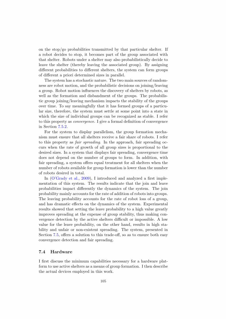
on the stop/go probabilities transmitted by that particular shelter. Ifa robot decides to stop, it becomes part of the group associated withthat shelter. Robots under a shelter may also probabilistically decide toleave the shelter (thereby leaving the associated group). By assigningdifferent probabilities to different shelters, the system can form groupsof different a priori determined sizes in parallel.

The system has a stochastic nature. The two main sources of random-ness are robot motion, and the probabilistic decisions on joining/leavinga group. Robot motion influences the discovery of shelters by robots, aswell as the formation and disbandment of the groups. The probabilis-tic group joining/leaving mechanism impacts the stability of the groupsover time. To say meaningfully that it has formed groups of a particu-lar size, therefore, the system must settle at some point into a state inwhich the size of individual groups can be recognized as stable. I referto this property as convergence. I give a formal definition of convergencein Section 7.5.2.

For the system to display parallelism, the group formation mecha-nism must ensure that all shelters receive a fair share of robots. I referto this property as fair spreading. In the approach, fair spreading oc-curs when the rate of growth of all group sizes is proportional to thedesired sizes. In a system that displays fair spreading, convergence timedoes not depend on the number of groups to form. In addition, withfair spreading, a system offers equal treatment for all shelters when thenumber of robots available for group formation is lower than the numberof robots desired in total.

In (O’Grady et al., 2009), I introduced and analyzed a first imple-mentation of this system. The results indicate that the join and leaveprobabilities impact differently the dynamics of the system. The joinprobability mainly accounts for the rate of addition of robots into groups.The leaving probability accounts for the rate of robot loss of a group,and has dramatic effects on the dynamics of the system. Experimentalresults showed that setting the leave probability to a high value greatlyimproves spreading at the expense of group stability, thus making con-vergence detection by the active shelters difficult or impossible. A lowvalue for the leave probability, on the other hand, results in high sta-bility and unfair or non-existent spreading. The system, presented inSection 7.5, offers a solution to this trade-off, so as to ensure both easyconvergence detection and fair spreading.

7.4 Hardware

I first discuss the minimum capabilities necessary for a hardware plat-form to use active shelters as a means of group formation. I then describethe actual devices employed in this work.

105

(a) (b)

Figure 7.1: The robot platforms I simulated for the experiments in this study.(a) The foot-bot; (b) the eye-bot.

7.4.1 Minimum Generic Requirements

An active shelter is capable of monitoring the number of grouped robotsover time, with coarse periodicity. In addition, it must be capable ofbroadcasting the join/leave probabilities to the robots in range. Finally,active shelters must be able to broadcast a 1-bit signal to nearby shelters.

A mobile robot must be capable of navigating the environment avoid-ing other robots. To coordinate the motion of robots joining/leavinga group as described in Section 7.5.2, each robot must convey 2-bitstate information (joined-group/leaving-group/free) to nearby robotsand shelters. A robot must detect the state of nearby robots and re-ceive the join/leave probabilities from the closest shelter. Finally, arobot must be able to perceive nearby robots.

7.4.2 Devices Used in This Study

In the experiments, I employed the foot-bot (Bonani et al., 2010) asmobile robot (Figure 7.1 (a)). The foot-bot navigates the environmentthrough a set of wheels and tracks called treels. It can convey its state(joined-group/leaving-group/free) through a colored LED ring that sur-rounds its body, and detect other robots’ state and relative locationthrough an omnidirectional camera.

To realize active shelters I used the eye-bot robot (Figure 7.1 (b)).The eye-bot (Roberts et al., 2007) is a quad-rotor robot able to attachto the ceiling. To detect mobile robots, the eye-bot is equipped with apan-and-tilt camera.

106

Group formation area

x0

x1 x2 x3

p1x0 l1x1 p2x0 l2x2 p3x0 l3x3

Figure 7.2: A schematic representation of the mathematical model describedin Section 7.5.1 with three active shelters.

Eye-bot–to–foot-bot and eye-bot–to–eye-bot communication occursthrough the range-and-bearing communication system (Roberts et al.,2009) present on all robots. This device allows the eye-bot to broadcasta message containing a 8-byte payload. The message can be received bynearby eye-bots and by foot-bots on the floor in a limited range.

The robots, as well as the range-and-bearing communication system,were developed in the Swarmanoid project (Dorigo et al., 2013).

7.5 Active Shelters

In this section, I present the system to achieve group formation controlthrough active shelters. I analyze its properties and identify its limita-tions. In Section 7.5.1, I present a mathematical model that capturesthe most important aspects of the system. In Section 7.5.2, I present thecomplete implementation of the system and analyze it through targetedphysics-based simulations.

7.5.1 Mathematical Model

The model.

In Figure 7.2, I illustrate the abstraction of the system upon which I basethe mathematical model. The shelters are distributed in a rectangulararea. The communication range of the shelters is displayed as a circulargray area. I assume that the communication ranges of a shelter do notoverlap with those of the other shelters. For the purposes of this model,I neglect the actual motion of the robots across the environment. Iassume that the robots perform a diffusion algorithm such as (Howardet al., 2002), so as to uniformly distribute in the environment. Thus,the probability c for a robot to be located within the communicationrange of a shelter is given by

c =Area(shelter)

Area(group formation area).

A robot joins the group of shelter i with probability ji. This probabilityis set by the active shelter depending on the desired group size. The

107

100

101

102

103

104

105

106

107

100 101 102 103 104 105

Len

gth

of p

hase

2 [

log]

Decay period [log]

[0.75,0.5,0.25][0.25,0.5,0.75]

Figure 7.3: Length of phase 2 in the simulations of the mathematical modelfor different values of the decay period δ.

probability pi for a robot to discover that shelter and join its group isgiven by pi = cji. The probabilities pi are assumed constant throughoutthe duration of a run.

A robot that is part of group i has a probability to leave it, denotedby li. As discussed in Section 7.3, setting li to a fixed value causes atrade-off between fair spreading with difficult convergence on one side,and stable convergence with unfair spreading on the other (O’Gradyet al., 2009). Thus, to reconcile convergence and spreading, the leaveprobability li must vary between a value that promotes fair spread-ing (hereinafter denoted by lhi), and a value that ensures convergence(hereinafter denoted by llow). At the beginning of the experiments, eachshelter i is configured with a probability li = lhi = 10−2. I thus ensurea good spread of robots early on in the group formation process. Overa period of time, each shelter exponentially decreases the value of its li,until it reaches llow = 10−5, thus allowing the system to gradually settleinto a stable state. More specifically, the values of the li’s are set asfollows:

li(t) = (lhi − llow)e−γt + llow, (7.1)

in which γ is the decay constant. I define γ as a function of a parameterδ that represents the number of time steps required by the exponentialto drop by 90%:

γ =ln 10

δ⇒ e−γδ = 0.1.

I denote the fraction of robots engaged in group i > 0 at time t as

108

0

0.2

0.4

0.6

0.8

1

T1=226

Rob

ot fr

actio

n

Time steps [log]

T2=7808

Shelt. 1Shelt. 2Shelt. 3

Free

T3=8124

(a) P1 = {0.75, 0.5, 0.25}; δshort = 102

0

0.2

0.4

0.6

0.8

1

T1=1265

Rob

ot fr

actio

n

Time steps [log]

T2=2712

Shelt. 1Shelt. 2Shelt. 3

Free

T3=4074

(b) P1 = {0.75, 0.5, 0.25}; δlong = 103

0

0.2

0.4

0.6

0.8

1

T1=249

Rob

ot fr

actio

n

Time steps [log]

T2=117692

Shelt. 1Shelt. 2Shelt. 3

Free

T3=117977

(c) P2 = {0.25, 0.5, 0.75}; δshort = 102

0

0.2

0.4

0.6

0.8

1

T1=1487

Rob

ot fr

actio

n

Time steps [log]

T2=3388

Shelt. 1Shelt. 2Shelt. 3

Free

T3=4750

(d) P2 = {0.25, 0.5, 0.75}; δlong = 103

Figure 7.4: Results with the mathematical model presented in Section 7.5.1.The experiments are composed of three phases. In phase 1, two shelters areactive. In phase 2 (starting at time T1), a third shelter is activated. In phase3 (starting at time T3), shelter 2 is deactivated. The experiment ends at timeT3. The length of each phase depends on the dynamics of the system. P1 andP2 account for the desired group size of each shelter. Parameter δ correspondsto the decay period for the probability to leave a shelter.

xi(t), and the free robots (i.e., not part of any group) as x0(t). Consid-ering the probabilities pi and li as rates of group joining and leaving,respectively, and denoting with n the number of shelters in the groupformation area, yields the following model:

x0(t + 1) = x0(t)−

(n∑

i=1

pi

)x0(t) +

n∑i=1

li(t)xi(t)

xi(t + 1) = xi(t) + pix0(t)− li(t)xi(t) (with i ∈ [1, n])

109

Model Behavior

To study the behavior of the model with respect to convergence andspreading, I set up a three-phase experiment. Initially, two sheltersform groups of different sizes for a certain period T1. At time t = T1, athird shelter is activated and it starts recruiting robots. Subsequently,at time t = T2, shelter 2 is disabled, thus freeing all the robots withinits group. The simulation ends at time t = T3.

The length of these three phases is not fixed, but depends on thedynamics of the system. To study convergence at each phase, I recordthe times T1, T2, and T3 in which the system reaches convergence ateach phase. Convergence is reached when all fractions (grouped andfree robots) change by a sufficiently little quantity. More precisely, Ideclare convergence at time t∗ if ∀k ∈ [0, n] |xk(t∗)− xk(t∗− 1)| < 10−6.

Whenever a new shelter is activated or deactivated spreading is im-portant to ensure fair resource distribution. The newly activated or de-activated shelter thus sends a signal to nearby shelters to notify them ofthe change to the system. The shelters react by forwarding this signalto their neighbors and resetting their leave probability value back to lhi.

To study spreading, I ran simulations with two different settings forthe values of the join probabilities: P1 = {0.75, 0.5, 0.25} and P2 ={0.25, 0.5, 0.75}. With P1, shelters 1 and 2 initially must recruit mostof the robots. Shelter 3 is the least demanding, so, upon its activationat time T1, the system must redistribute only a few robots to shelter 3.Conversely, with P2, shelter 3 is the most demanding. Its activation att = T1 forces the system to redistribute most of the robots.

I ran several experiments with different values for parameter δ. Theexperiments revealed that the most problematic event in the setting isthe addition of shelter 3 at the beginning of phase 2. As reported inFigure 7.3, the length of this phase decreases with the increase of thedecay period in the range [101, 103]. For δ = 104, the length of phase 2slightly increases with respect to δ = 103.

A sample of the dynamics of the system for different values of δ isreported in Figure 7.4. In these experiments, I tested δ = δshort = 102

and δ = δlong = 103 time steps. As the plots show, the length ofthe decay period of the leave probability has a strong impact on thebehavior of the system and the values of T1, T2 and T3. If the decayperiod is short (δ = δshort), the value of the leaving probability dropsquickly and the system behavior results in unfair spreading and verylong convergence times. A long decay period (δ = δlong), on the otherhand, has a positive effect on both properties, because the robots havesufficient time to spread across the shelters.

110

7.5.2 Physically Simulated Robot

Implementation

I performed experiments using ARGoS to validate the predictions of themodel in a physically realistic robotic system. A prominent aspect thataffects the system performance is interference among mobile robots. Inthe system, interference occurs mainly under the active shelters. Themobile robots must organize in tight aggregates under the shelters, whilepermitting the flow of leaving and joining robots.

In the physics-based simulations, I assume that the robots are ran-domly distributed in a group formation area in which shelters are dis-tributed. At any moment, a robot performing random walk across theenvironment can either be under a specific shelter or in a shelter-freearea. The robot behavior is described by the simple state machine re-ported in Figure 7.5. The meaning of the states are as follows:

• state free: A robot does not belong to any group. The robot per-forms random walk with obstacle avoidance. This state is conveyedwith LEDs lit up in green.

• state in group: A robot is part of a group. This state is conveyedwith LEDs lit up in red.

• state leaving: A robot is leaving a group to which it previouslybelonged. This state is conveyed with LEDs lit up in blue.

Join probability

When a robot in state free enters the communication range of shelteri, it transitions to state in group with probability ji. This probabilityis related to the target group size qi associated to the shelter. I aim tofind a simple relationship between ji and qi. The communication rangeof a shelter is limited in size and, thus, can house a maximum numberof robots, which I denote with f . I assume that all the shelters haveidentical communication ranges, so f is a constant across the sheltersknown a priori. In addition, I assume that the target group sizes qi

cannot exceed f . Each shelter constantly monitors the number of robotscurrently engaged in its group. If the group size exceeds the target size,the shelter must stop recruiting robots. From these considerations, Iderive the following simple definition for ji:

ji =

{qi/f if current size of group i < qi,

0 otherwise.

111

Cfree−>free Cin_group−>in_group

leaving−>freeC

Cleaving−>leaving

Cin_group−>leaving

Cin_group−>free

Cfree−>in_group

LEAVING

IN_GROUPFREE

State transition conditionsCfree→in group JustInRange() = true and Rand() ≤ ji

Cfree→free InRange() = false or (JustInRange() = trueand Rand() > ji)

Cin group→free InRange() = falseCin group→leaving InRange() = true and Rand() ≤ liCin group→in group InRange() = true and Rand() > liCleaving→free InRange() = falseCleaving→leaving InRange() = true

Figure 7.5: State transition logic for robots at each time step. InRange()and JustInRange() are functions returning true when the robot is within thecommunication range of a shelter, and has just entered it, respectively. Rand()is a function returning a random number in U(0, 1). ji is the join probability forshelter i, li is the leave probability. State transition conditions are representedbe the symbol C and a subscript. For example, Cin group→in group representsthe conditions under which an aggregated robot will stay aggregated in itsgroup in a single time step.

Leave Probability

A robot in state in group beneath shelter i transitions to state freewith probability li. The probability li decays exponentially follow-ing (7.1).

Robots Joining and Leaving a Group

Physical interference among grouped robots may have severe effects onthe system, especially when the density of robots under a shelter be-comes high. Upon deciding to leave, a robot located in the center ofa group needs a clean path out of it. However, if the area beneath ashelter is crowded, the formation of the exit path is likely to push somerobots located at the border of the group out of the communication area,thus losing contact with the shelter. Thus, interference reduces stability,especially in large groups.

112

C1

C2 C3 C1 C3

Shelter 1 Shelter 2 Shelter 3

0

5

10

15

20

0

5

10

15

20

0

0.25

0.5

0.75

1

Gro

up S

ize

Gro

up S

ize

Avg

Avg

/ D

esire

d G

roup

Siz

e

0 T1 1000 2000 T2 3000 4000 5000

Time [sec]

D1

D2

D3

D1

D2

D3

(a) Target sizes: [15, 10, 20]

Shelter 1 Shelter 2 Shelter 3

0

5

10

15

20

0

5

10

15

20

0

0.25

0.5

0.75

1

Gro

up S

ize

Gro

up S

ize

Avg

Avg

/ D

esire

d G

roup

Siz

e

C1

C2C3

C1C3

0 T1 1000 2000 T2 3000 4000 5000

Time [sec]

D1,D2,D3

D1,D2,D3

(b) Target sizes: [12, 12, 12]

Figure 7.6: Results with physically simulated robots following the behaviorexplained in Section 7.5.2. The experiments are composed of three phases. Inphase 1, two shelters are active. In phase 2 (starting at time T1), a third shelteris activated. In phase 3 (starting at time T2), shelter 2 is deactivated. Theexperiment ends at time T3. The top plots shows a representative experimentalsample in the pool of the 100 repetitions I ran. The middle plot reports theaverage system behavior. The bottom plot shows the ratio between the currentand the desired group size. 113

To solve these issues, I consider each robot to be immersed in twovirtual potential fields (Spears et al., 2004). The first field attractsrobots that decide to be part of a group towards the center of suchgroup, or repels those who decide to leave the group. The second fieldallows a robot that decides to leave the group to push its way out withoutdisrupting the integrity of the group.

Convergence Detection

It is important for a shelter to be able to detect convergence. However,due to the probabilistic nature of the system, the group size displayscontinuous fluctuations. Thus, the notion of convergence to a targetgroup size must be linked to these fluctuations. Intuitively, a shelter candeclare convergence when the magnitude of the fluctuations remains fora certain period of time within a specific range.

In practice, each shelter monitors the fluctuations of the number ofits aggregated robots over a period of time TC . If the magnitude of thefluctuations stays within some tolerance boundaries for the entire pe-riod, the shelter considers the system to have converged. The toleranceboundary B is defined as a function of the leave probability llow, thelength of the monitoring period TC and the size of the aggregate gi atthe beginning of the monitoring period:

B =√

TCgillow(1− llow)

B is derived by considering the changing number of aggregated robotsunder a shelter as a time series produced by a binomial distribution inwhich p = llow. B is calculated as the standard deviation of such a timeseries over the monitoring period TC .

7.5.3 Experimental Evaluation

Experimental Setup

I ran experiments with a 3-phase setup analogous to what I presented forthe mathematical model. The values of T1 = 50 s, T2 = 250 s, and T3 =500 s were chosen to give the system sufficient time to reach convergenceat each stage.

I distributed 30 robots in the group formation area. In the first phase,the target sizes of shelter 1 and 2 are always set so that their sum is lessthan 30. This first phase therefore allows us to test whether the systemis capable of converging to the correct group sizes in the simple casewhere there are enough robots to satisfy all target sizes. The secondphase, in which also shelter 3 is activated, tests the spreading propertyof the system in response to the activation of new shelters. In particular,I set shelter 3’s target size to make the sum of the target sizes greater

114

than the total number of robots in the group formation area. The thirdand final phase tests the spreading property of the system, this time inresponse to the release of robots by shelter 2. The convergence propertyof the system is tested in all three phases of the experiments.

For the experiments in this section, I tested two target size configu-rations: [15, 10, 20] and [12, 12, 12]. In the first configuration, shelter 3’starget size is greater than those of shelter 1 and shelter 2, thus requiringthe system to redistribute robots. This corresponds to setting P2 of theexperiments with the mathematical model. The second configurationwas chosen to specifically assess the spreading property. For the decayperiod, I selected the value δ = δlong = 103.

Results

The results are reported in Figure 7.6. The plots show that convergenceis reached in both experimental settings, regardless of desired groupsizes. The detection of convergence in phase 2, which is the most criticalphase in the experiment, is achieved by all robots within slightly lessthan 10 simulated minutes from the beginning of the phase.

Regarding spreading, the bottom plots of Figures 7.6(a)-(b) showthe average fulfilling percentage of the groups. In both experimentalsettings, regardless of the desired group size, these percentages stabilizeon the same value in all phases.

7.6 Scalability Assessment

One of the key motivations to create a new group formation mechanismis to achieve scalability (see Section 7.2). This motivation is the drivingforce behind the choice of a decentralized cockroach-inspired model. Inthis section, I test the scalability properties of the approach. I conductexperiments with hundreds of mobile robots that must be divided indozens of groups. Parallel group formation with these numbers wouldbe difficult to achieve with existing group formation approaches.

7.6.1 Experimental Setup

The shelters are distributed in a N×N grid. I set the desired group sizeto 25 for all the shelters. The experimental setup is shown in Figure 7.7.Figure 7.7 (a) is a snapshot of the simulated group formation area.Figure 7.7 (b) is an abstract representation of the same group formationarea in which the gray intensity of each square is proportional to thenumber of grouped robots. This representation allows for visual analysisof the sizes of the groups and their spatial distribution in the groupformation area over time.

115

Figure 7.7: Snapshot from scalability experiments with physically simulatedrobots. Left: Simulation snapshot. Right: Abstracted representation of thissimulation snapshot—the gray intensity level of each square is proportional tothe recruited group size of the correspondingly positioned shelter (i.e., to thenumber of robots recruited by that shelter).

In all the experiments, I set the number of available mobile robotsto 20N2. In this way, if fair spreading occurs, at convergence, a groupof 20 robots should have been formed under each shelter.

7.6.2 Convergence

In this section, I present a set of experiments designed to test the con-vergence property of the system. I ran experiments with 16 and 25shelters (320 and 500 mobile robots, respectively). The duration of eachexperiment was set to 750 s.

The results are reported in Figure 7.8. The top plots shows thedynamics of a sample run taken at random from the 80 experiment rep-etitions. I also display three snapshots at 250 s, 500 s and 750 s. Afteran initial period of instability, in which the group sizes grow with largefluctuations, the system converges in both experimental settings. Thelength of the decay period δ in these experiments was set to 350 s, whichexplains the duration of the fluctuating phase, about 400 s. At conver-gence, for both experimental settings, the distribution of the group sizesis centered around the target value of 20. In particular, the median ofthe group size distribution is 21. With 16 shelters, the first quartile ofgroup size is 14 and the third quartile is 23, while with 25 shelters theinter-quartile extrema are 15 and 25.

The average behavior of the system over 80 runs, showed by thebottom plots of Figure 7.8, confirms these observations. The median ofthe formed groups grows to 22, and the extrema of the inter-quartilerange of the final sizes I observed are 15 and 25.

The plots also show that the time to reach convergence is very similarwith 16 and 25 shelters. The convergence time of the system appears tobe practically independent of the number of robots, thus confirming thatthe proposed group formation mechanism displays the spreading prop-

116

erty. This result is expected because the system is completely paralleland based on local interactions among mobile robots and shelters.

7.6.3 Spreading

To test spreading, I devised a two-phase experimental setting. In thefirst phase, the system is given 750 s to reach convergence. At the be-ginning of the second phase, I activate or deactivate a shelter. Theseevents force the system to redistribute the mobile robots and reach anew convergence state, thus providing a good test of how capable thesystem is of spreading robots between shelters. The length of the secondphase is set to 750 s.

As I explained in Section 7.5, upon activation and deactivation, ashelter broadcasts a signal to its neighbors. The neighbors of a shelterare those shelters in direct line of sight. The signal forces the recipientsto reset the leaving probability to lhi and to restart the decay process.

An important aspect in the system is the transmission range of thereset signal. In Section 7.6.3, I analyze the results I obtained in ex-periments in which the reset signal is broadcast globally throughoutthe system. In Section 7.6.3, I discuss the results I obtained when thetransmission range of the signal is limited.

Global Reset Signal

In this section, I analyze the results I obtained with a global broadcast ofthe reset signal across the shelters. In these experiments I use 9 sheltersand 180 robots.

To study whether the starting point of the (de)activation event affectsthe system behavior, I explore the cases in which the event occurs atthe corner and at the center of the shelter grid.

The results are reported in Figures 7.9 and 7.10. In all the experi-mental settings, at the end of phase 1 the system reaches convergence toa state in which the group size distribution is tightly packed around thetarget value 20. The event causes the shelters to release the groupedrobots. The subsequent dynamics, in the average plots, shows that,regardless of the location of the event and its type (activation/deacti-vation), the system is able to reach a new convergence state. The finaldistribution of the group sizes is tightly packed around 20 robots.

The snapshots in Figures 7.9 and 7.10 of the sample experimentsshow that the initial location of the event does not affect the final dis-tribution of the robots. The gray levels in the snapshot do not displayany visible bias towards a specific region of the group formation area,thus indicating that spreading is fair.

117

0 5 10 15 20 25 30

250 500 750 0 5 10 15 20 25 30

Gro

up s

ize

Time [sec]

Min - Max1Q - 3Q

250 500 750 0 5 10 15 20 25 30

Gro

up s

ize

Time [sec]

T = 250 T = 500 T = 750

Min - Max1Q - 3Q

(a) 16 shelters, 320 mobile robots.

0 5 10 15 20 25 30

250 500 750 0 5 10 15 20 25 30

Gro

up s

ize

Time [sec]

Min - Max1Q - 3Q

250 500 750 0 5 10 15 20 25 30

Gro

up s

ize

Time [sec]

T = 250 T = 500 T = 750

Min - Max1Q - 3Q

(b) 25 shelters, 500 mobile robots.

Figure 7.8: Scalability experiments testing the convergence and spreading prop-erties of the system. Results are shown for two sets of experiments with 16shelters (a) and 25 shelters (b). 80 experimental runs per set of experiments.The top plots show the behavior of the system in a single sample experimentthat I have selected. The grids of squares represent snapshots of the state ofthe system at given moments in time during this sample experiment. The grayintensity of each individual square corresponds to the number of mobile robotsrecruited at that time by a single shelter. The min-max lines show the sizeof the largest recruited group of mobile robots and the size of the smallestrecruited group of foot-bots at any given moment. The 1Q and 3Q lines showthe inter-quartile range of the distribution of recruited group sizes among theshelters. The 1Q is the first quartile and shows the minimum recruited groupsize once I discard the lowest 25% of groups. The 3Q line is the third quartile,and shows the maximum recruited group size once I discard the highest 25%of the data. The bottom plot shows the same data averaged over all 80 runs.

118

0 5 10 15 20 25 30

250 500 750 1000 1250 1500 0 5 10 15 20 25 30

Gro

up s

ize

Time [sec]

Min - Max1Q - 3Q

250 500 750 1000 1250 1500 0 5 10 15 20 25 30

Gro

up s

ize

Time [sec]

T = 250 T = 500 T = 750 T = 1000 T = 1250 T = 1500

Min - Max1Q - 3Q

(a) Corner robot activates at time 750 s

0 5 10 15 20 25 30

250 500 750 1000 1250 1500 0 5 10 15 20 25 30

Gro

up s

ize

Time [sec]

Min - Max1Q - 3Q

250 500 750 1000 1250 1500 0 5 10 15 20 25 30

Gro

up s

ize

Time [sec]

T = 250 T = 500 T = 750 T = 1000 T = 1250 T = 1500

Min - Max1Q - 3Q

(b) Center robot activates at time 750 s

Figure 7.9: Set of experiments testing the spreading property of the system.All experiments run with 9 shelters and 180 mobile robots in a recruitmentarea consisting of a 3x3 shelter formation. Results are shown for two sets ofexperiments. Each experimental run lasts for 1,500 s. 20 experimental runswere conducted for each set of experiments. Top plots in each set representselected sample runs, while bottom plots represent data averaged over all 20runs. For a more detailed explanation of the plots see previous caption fromFigure 7.8.

119

0 5 10 15 20 25 30

250 500 750 1000 1250 1500 0 5 10 15 20 25 30

Gro

up s

ize

Time [sec]

Min - Max1Q - 3Q

250 500 750 1000 1250 1500 0 5 10 15 20 25 30

Gro

up s

ize

Time [sec]

T = 250 T = 500 T = 750 T = 1000 T = 1250 T = 1500

Min - Max1Q - 3Q

(a) Center robot deactivates at time 750 s

0 5 10 15 20 25 30

250 500 750 1000 1250 1500 0 5 10 15 20 25 30

Gro

up s

ize

Time [sec]

Min - Max1Q - 3Q

250 500 750 1000 1250 1500 0 5 10 15 20 25 30

Gro

up s

ize

Time [sec]

T = 250 T = 500 T = 750 T = 1000 T = 1250 T = 1500

Min - Max1Q - 3Q

(b) Corner robot deactivates at time 750 s

Figure 7.10: Set of experiments testing the spreading property of the system.All experiments run with 9 shelters and 180 mobile robots in a recruitmentarea consisting of a 3x3 shelter formation. Results are shown for two sets ofexperiments. Each experimental run lasts for 1,500 s. 20 experimental runswere conducted for each set of experiments. Top plots in each set representselected sample runs, while bottom plots represent data averaged over all 20runs. For a more detailed explanation of the plots see previous caption fromFigure 7.8.

120

Local Reset Signal

Although a global reset signal allows for fair spreading after the ac-tivation and deactivation of shelters, its application to real scenariosis problematic. In fact, if the frequency of these events is too high,the system may have insufficient time to reach convergence, resultingin constantly fluctuating group sizes. To prevent constant fluctuations,the convergence results of Section 7.6.2 suggest that the time betweenactivation/deactivation events must be greater than the decay periodδ. As the size of the scenario grows, and with it the number of groupformation requests per time unit, the frequency of the events is likely toexceed δ−1, thus causing constant fluctuations. A possible solution tothis problem is to limit the range of transmission of the reset signal.

In this series of experiments, I test the impact on the spreading abilityof the system when the reset signal is not globally broadcast. I use16 and 25 shelters (to which correspond 320 and 500 mobile robots,respectively) and deactivate only one corner shelter.

Short range. Figure 7.11 shows the results of experiments in whichthe reset signal was transmitted only to the closest neighbors of a per-turbed shelter (i.e., the shelters in the Moore neighborhood). The finalstate reached by the system presents two regions, one affected by theperturbation and one not affected by it. In the region affected by theperturbation, the final group sizes are visibly lower than in the otherregion. Thus, spreading is not fair. This phenomenon can be explainedby observing that, upon leaving a group, the direction chosen by a robotis random and uniformly distributed. Thus, part of the robots leakedfrom the perturbed region to the unperturbed one.

Medium range. Figure 7.12 shows the results of experiments in whichthe reset signal was transmitted in a medium range. The reset signalreaches the neighbors of the neighbors of the originally perturbed shel-ter. Analogously to the previous case, the final state of the system ischaracterized by two regions, one affected by perturbation and one notaffected. Since a larger part of the system takes part into the redistri-bution process, the distribution of the final group size is more even thanthe non-propagated signal case, but still spreading is not very fair.

Discussion

The communication range of the reset signal characterizes the abilityof the system to redistribute the robots. The experiments show that,when the frequency of the perturbations exceeds δ−1, limiting the rangeof the reset signal is not enough, by itself, to ensure fair redistribution.This problem is due to the fact that the robots that leave the perturbed

121

0 5 10 15 20 25 30

250 500 750 1000 1250 1500 0 5 10 15 20 25 30

Gro

up s

ize

Time [sec]

Min - Max1Q - 3Q

250 500 750 1000 1250 1500 0 5 10 15 20 25 30

Gro

up s

ize

Time [sec]

T = 250 T = 500 T = 750 T = 1000 T = 1250 T = 1500

Min - Max1Q - 3Q

(a) 16 shelters, 320 mobile robots.

0 5 10 15 20 25 30

250 500 750 1000 1250 1500 0 5 10 15 20 25 30

Gro

up s

ize

Time [sec]

Min - Max1Q - 3Q

250 500 750 1000 1250 1500 0 5 10 15 20 25 30

Gro

up s

ize

Time [sec]

T = 250 T = 500 T = 750 T = 1000 T = 1250 T = 1500

Min - Max1Q - 3Q

(b) 25 shelters, 500 mobile robots.

Figure 7.11: Set of experiments on local perturbation. In these experiments,the propagation of the reset signal is limited to the direct neighbors. Results areshown for two sets of experiments (a,b). 20 experimental runs were conductedfor each set of experiments. Each experimental run lasts 1,500 s. Top plotsin each set represent selected sample runs, while bottom plots represent dataaveraged over all 20 runs. For a more detailed explanation of the plots seeprevious caption from Figure 7.8.

122

0 5 10 15 20 25 30

250 500 750 1000 1250 1500 0 5 10 15 20 25 30

Gro

up s

ize

Time [sec]

Min - Max1Q - 3Q

250 500 750 1000 1250 1500 0 5 10 15 20 25 30

Gro

up s

ize

Time [sec]

T = 250 T = 500 T = 750 T = 1000 T = 1250 T = 1500

Min - Max1Q - 3Q

(a)

0 5 10 15 20 25 30

250 500 750 1000 1250 1500 0 5 10 15 20 25 30

Gro

up s

ize

Time [sec]

Min - Max1Q - 3Q

250 500 750 1000 1250 1500 0 5 10 15 20 25 30

Gro

up s

ize

Time [sec]

T = 250 T = 500 T = 750 T = 1000 T = 1250 T = 1500

Min - Max1Q - 3Q

(b)

Figure 7.12: Set of experiments on local perturbation. In these experiments,the propagation of the reset signal is limited to the second-level neighbors (i.e.,the direct neighbors of the direct neighbors of the signal originator). Results areshown for two sets of experiments (a,b). 20 experimental runs were conductedfor each set of experiments. Each experimental run lasts 1,500 s. Top plotsin each set represent selected sample runs, while bottom plots represent dataaveraged over all 20 runs. For a more detailed explanation of the plots seeprevious caption from Figure 7.8.

123

shelters tend to leave the group in all the directions. As a consequence,only a part of the leaving robots are directed towards other perturbedshelters. The other robots join already stable groups. In this way, tworegions are formed in the system—one region with a surplus of robots,and a region with a deficit of robots. A possible solution for this problem,currently under study, is to prevent the robots from navigating towardsthe unperturbed regions of the system.

Summary

In this chapter I presented a novel, distributed approach to the formationof multiple groups of mobile robots. The main feature of the algorithmis the ability to fairly distribute robots across group of different targetsizes even in presence of scarce resources. The method takes inspirationfrom the behavior of cockroach aggregation under shelters. In the sys-tem, shelters are simple, active devices able to monitor the number ofaggregated robots, and calculate and locally broadcast probabilities forthe robots to join and leave the aggregate.

I showed that the stability of the groups is mainly dependent on theleaving probability, and presented a system in which shelters vary thisprobability over time to control group size. I demonstrated that, toachieve group size convergence and fair robot spreading, it is sufficientto let the leaving probability decay gradually from a high value to a lowvalue.

I assessed the performance of the system in a large, challenging sce-nario in which hundreds of robots must be aggregated into dozens ofgroups. The results suggest that, due to its parallelism, the convergencetime of the system is basically independent of the size of the scenario.Regarding spreading, the system is able to distribute the robots evenlyamong the shelters. In presence of perturbations, such as activation/de-activation of a shelter, spreading is fair if the time between two of theseevents is longer than the decay period of the leaving probabilities.

Future work involves studying methods to modify the system to en-hance spreading with a high frequency of perturbations. A possible wayto improve the system is to keep the propagation of the perturbationslocal, and prevent the robots that are temporarily freed from leaking tothe non-perturbed region.

124

Chapter 8

Conclusions and Future Work

The long-term vision for swarm robotics applications is extremely di-verse. Construction, search-and-rescue, space exploration, and surgeryare but a few of the many applications foreseen in the distant future.At present, however, developing effective swarm robotics systems is adifficult endeavor due to the lack of general methodologies. Successfulattempts to design these systems concentrate on specific scenarios, withlittle opportunity for generalization.

One of the most crucial hurdles to develop a general methodologyfor the design of swarm robotics systems is the lack of dedicated de-velopment tools. Development tools, such as simulators, programminglanguages, and robot platforms, constitute the backbone around whichmethodologies are conceived and validated.

This thesis deals with ARGoS, the first physics-based robot simula-tor specifically designed for swarm robotics applications. The facetednature of swarm systems entails three main requirements: (i) accuracy,to ensure satisfactory correspondence between the results predicted bythe simulation and the results obtained through real-world experiments;(ii) flexibility, to support any kind of robot and experiment; and (iii)efficiency, to minimize the time necessary to complete a simulation.

In the design of ARGoS, I have considered accuracy not as an intrinsicproperty of the simulator, but as a measurable quantity whose thresholdof acceptance is decided by the experimenter. Consequently, in ARGoSaccuracy is tunable. Accuracy tuning consists in choosing the modelsinvolved in a simulation. Models are encapsulated into modules, thatthe user selects as part of the configuration of the experiment. To thisend, the architecture of ARGoS offers unprecedented levels of modular-ity, allowing the user to override any aspect of the simulation: sensors,actuators, physics engine, communication media, and visualizations.

Flexibility is a direct consequence of ARGoS’ modularity. A uniquefeature of ARGoS is the possibility to execute the simulation using mul-tiple physics engines, dedicating each engine to a portion of the physical

125

space. In addition, ARGoS is implemented as a library with a power-ful API, which renders embedding it into larger applications easy andfast. For instance, ARGoS has been interfaced to genetic algorithms toperform evolutionary robotics experiments.

Efficiency in ARGoS is obtained through a wide set of techniques anddesign choices that span multiple levels of the architecture. Tunable ac-curacy allows the user to assign computational resources to the relevantaspects of a simulation, and to employ less accurate (and, thus, faster)models for unimportant aspects. Differently from any existing simula-tor, in ARGoS, spatial indexing is implemented as a policy. This allowsthe user to select the best spatial index for the experiment at hand.Additionally, multi-threading ensures a good use of modern, multi-corearchitectures. A unique feature of ARGoS in this respect is the possi-bility to choose the scheduling strategy for assigning tasks to threads.

Experimental evaluation demonstrates that ARGoS is capable of sim-ulating thousands of robots in a fraction of real time. In particular,experiments on an average computer show that ARGoS can complete anavigation experiment involving 10,000 robots in 60% of real-time —anunmatched result in the literature so far.

ARGoS is open source software released under the terms of the MITlicense. Over the years, it has been employed for a large number ofresearch works in swarm robotics including navigation, pattern forma-tion, self-assembly, foraging, task allocation, and construction. At themoment of writing, ARGoS is used in 15 laboratories worldwide, andit is the official robot simulator of the projects Swarmanoid, ASCENS,E-SWARM, H2SWARM, and Swarmix. A little community of contrib-utors is providing support in the form of bug reports and third-partyextensions. For instance, ARGoS has been integrated by Kudelski et al.(2013) with the well-known network simulator ns3,1 producing the firstsoftware capable of both simulating the physics and the WiFi commu-nication capabilities of a robot swarm accurately.

Future work on ARGoS will follow several directions. One directionis to further improve its performance, possibly reaching hundreds ofthousands of robots in real time. One possible way to achieve this resultis integrating ARGoS with data structures that exploit the graphicalprocessing unit (GPU) onboard any modern personal computer. Ad-ditionally, the architecture of ARGoS could be redesigned to be multi-process as well as multi-threaded. Multi-process architectures are al-ready employed by several simulators, such as Gazebo and Morse. How-ever, multi-processing in these simulators is implemented as a central-ized system in which a special node coordinates the operations of theother nodes. To improve performance, a possible alternative could be a

1https://www.nsnam.org/

126

peer-to-peer architecture, in which nodes exchange information directly,without the need for a centralized coordinator.

Another direction for future work is integrating ARGoS with othertools, such as programming languages and analysis tools. Regarding lan-guages, users can now program robot control code in C++, ASEBA, andLua, and integration with languages such as Proto and ROS is planned.Furthermore, ARGoS will soon be integrated with the advanced statis-tical analyzer MultiVeStA (Sebastio and Vandin, 2013).

Last but not least, effort will be put in the integration of more robotsand more experimental modalities. For instance, realistic models forunderwater experiments, and voxel-based physics engines to simulateshores and construction with deformable materials are currently understudy. Additionally, improved support for modular robots, magnetism,and articulated robots is currently being developed.

Looking forward, my hope is that ARGoS will play an increasinglyimportant role in the development of swarm robotics. In particular, byits very nature, ARGoS is suitable to tackle research questions that havereceived little attention so far. Among these questions, I believe thatthree are paramount: (i) how to realize effective human-swarm interac-tion, that allows an operator to influence the behavior of an autonomousswarm in tasks such as search-and-rescue, exploration, and construction;(ii) how to develop, debug, and maintain large-scale swarm behaviors;and (iii) how to establish general benchmarks to characterize and com-pare existing approaches, thus fostering the emergence of best practicesand solid methodologies.

127

Appendix A

Other Scientific Contributions

Over the course of my doctorate, I have conducted a number of studiesnot directly related to the main topic of this thesis. These works touchseveral topics, and can be divided into two categories: swarm roboticsand Boolean network robotics.

A.1 Swarm Robotics

A.1.1 Pattern Formation and Flocking

• C. Pinciroli, M. Birattari, E. Tuci, M. Dorigo, M. Del Rey Zapa-tero, T. Vinko, D. Izzo. Self-Organizing and Scalable ShapeFormation for a Swarm of Pico Satellites. Proceedings of theNASA/ESA Conference on Adaptive Hardware and Systems (AHS-2008). IEEE-CS Press, Washington, DC, USA, pages 57–61, 2008.

• C. Pinciroli, M. Birattari, E. Tuci, M. Dorigo, M. Del Rey Za-patero, T. Vinko, D. Izzo. Lattice Formation in Space fora Swarm of Pico Satellites. The Sixth International Confer-ence on Ant Colony Optimization and Swarm Intelligence (ANTS-2008). Springer LNCS 5217, Berlin, Germany, pages 347–354,2008.

Pattern formation is an activity whereby mobile robots displace them-selves autonomously so as to form a predefined shape. In these works,we have explored the problem of forming patterns with small satellitesorbiting a planet.

• A. Stranieri, E. Ferrante, A. E. Turgut, V. Trianni, C. Pinciroli,M. Birattari, M. Dorigo. Self-Organized Flocking with a Het-erogeneous Mobile Robot Swarm. Advances in Artificial Life(ECAL 2011). MIT press, Cambridge, MA, pages 789–796, 2011.

• E. Ferrante, A. E. Turgut, C. Huepe, A. Stranieri, C. Pinciroli,M. Dorigo. Self-Organized Flocking with a Mobile Robot

129

Swarm: a Novel Motion Control Method. Adaptive Behav-ior, 20(6):460–477, 2012.

While pattern formation aims to create a static shape, the purpose offlocking is to coordinate the motion of a group of mobile robots towardsa target location. As a result of coordination, the robot swarm movesas a unique entity.

An important research question is whether explicit alignment nego-tiation among the robots is required to achieve flocking. To shed lighton this question, I have cooperated to two works. In the first, therobot swarm is divided in two groups, aligning and non-aligning. Align-ing robots exchange information to negotiate a direction; non-aligningrobots lack this capability. Results show that indeed flocking is possi-ble even in presence of non-aligning robots, but flocking performanceincreases with the fraction of aligning ones. In the second work, wemoved our attention to an overlooked aspect of the flocking mechanism—motion control. Motion control is the component that translates theproximal and alignment components into actual movement. We pro-posed a novel motion control rule, which increases flocking performancesensibly with non-aligning robots.

• E. Ferrante, A. E. Turgut, A. Stranieri, C. Pinciroli, M. Birattari,M. Dorigo. A Self-Adaptive Communication Strategy forFlocking in Stationary and Non-Stationary Environments.Natural Computing, 2014. In press.

In another work, we explored the case in which a small group ofrobots in a swarm possesses information regarding the target location,and must guide the rest of the swarm. We proposed an algorithm thatallows the robots to flock in the following conditions: (i) the targetlocation is constant over time; (ii) the target location changes over time;(iii) two groups of robots have information about contrasting targetlocations.

The experiments on flocking have been conducted with ARGoS, bothin simulation and with real robots.

A.1.2 Cooperative Navigation

• F. Ducatelle, G. Di Caro, C. Pinciroli, F. Mondada, L. M. Gam-bardella. Communication Assisted Navigation in RoboticSwarms: Self-Organization and Cooperation. Proceedingsof the IEEE/RSJ International Conference on Intelligent Robotsand Systems (IROS 2011). IEEE Computer Society Press, LosAlamitos, CA, pages 4981–4988, 2011.

In this set of works, we investigated distributed methods to route in-dividual robots towards a destination. All these method revolve around

130

the idea that robots form a network. Depending on the position ofthe robots with respect to the target locations, these methods dictatehow information flows in the network, in order to guide a robot to itsdestination.

We investigated the idea of guiding wheeled robots using a swarmof flying robots. The wheeled robots are unaware of the structure ofthe environment and must navigate between two locations. To optimizethe path followed by the wheeled robots, the flying robots adapt theirposition over time to the motion of the wheeled robots. To the best of ourknowledge, this method is the first example of self-organized cooperationin a physically heterogeneous swarm.

• F. Ducatelle, G. Di Caro, C. Pinciroli, L. M. Gambardella. Self-Organised Cooperation between Robotic Swarms. SwarmIntelligence, 5(2):73–96, 2011.

• F. Ducatelle, G. Di Caro, A. Forster, M. Bonani, M. Dorigo,S. Magnenat, F. Mondada, R. O’Grady, C. Pinciroli, P. Retornaz,V. Trianni, L. M. Gambardella. Cooperative Navigation inRobotic Swarms. Swarm Intelligence, available at http://link.springer.com/article/10.1007%2Fs11721-013-0089-4#page-1,2013.

In the above method, the wheeled robots use information from theflying robots to navigate. The fact that the flying robots adapt theirposition to the motion of the wheeled robots can be interpreted as a way,for the wheeled robots, to achieve a form of stigmergic communication.

In subsequent works, we studied methods based on other forms ofcommunication to produce behaviors that achieve cooperative naviga-tion. In particular, we concentrated on the problem of routing a homo-geneous swarm of wheeled robots between two locations, maintainingthe assumption that the robots do not possess nor construct an explicitrepresentation of the environment.

We proposed a method inspired by routing algorithms in mobile adhoc networks. Each robot maintains a routing table containing theshortest path to each known target location. The target locations arefirst discovered by the robots that can perceive it directly. The informa-tion on a target location is broadcast periodically and propagated by allrobots throughout the network. This algorithm allows a single robot tobe routed to a specific destination. In addition, when the entire swarm isrequired to navigate between two points, this algorithm autonomouslyconverges to a chain-like formation between the two locations. Thisswarm behavior occurs also in presence of obstacles.

• A. Gutierrez, A. Campo, F. C. Santos, C. Pinciroli, M. Dorigo. So-cial Odometry in Populations of Autonomous Robots. TheSixth International Conference on Ant Colony Optimization and

131

Swarm Intelligence (ANTS-2008). Springer LNCS 5217, Berlin,Germany, pages 371–378, 2008.

In a further paper, we show that a similar chaining behavior can beobtained if robots exchange distance information estimated from odom-etry data. Since the error of this estimate increases with the distancefrom the target, the robots communicate the level of confidence alongwith the information on the distance. This paper shows that this sim-ple mechanism is sufficient to achieve a stable chain between two targetlocations.

All the above experiments have been conducted with ARGoS, bothin simulation and with real robots.

A.1.3 Self-Assembly

• R. O’Grady, C. Pinciroli, R. Groß, A. L. Christensen, F. Mondada,M. Bonani, M. Dorigo. Swarm-bots to the Rescue. EuropeanConference on Artificial Life (ECAL 2009). Springer LNCS 5777,Berlin, Germany, pages 165–172, 2009.

In self-assembly, groups of robots connect to each other to performtasks that would not be feasible individually.

One of today’s open problems in self-assembly is when to trigger theself-assembling process. In this paper, we propose an algorithm thatallows robots to decide between performing a task individually and co-operating by forming physical connections to other robots. We test ouralgorithm in rescue scenario in which broken robots must be transportedto safety by rescuer robots. Each broken robot requires a different num-ber of rescuers to be transported. The algorithm assumes that rescuersare not aware a priori of the required number of robots to complete atransport.

• R. O’Grady, A. L. Christensen, C. Pinciroli, M. Dorigo. RobotsAutonomously Self-Assemble into Dedicated Morpholo-gies to Solve Different Tasks. Proceedings of the 9th Interna-tional Conference on Autonomous Agents and Multiagent Systems(AAMAS 2010). International Foundation for Autonomous Agentsand Multiagent Systems, Richland, SC, pages 1517–1518, 2010.

In this work, we investigated another important open problem in self-assembly: Which morphology must be selected for a given task? Theresult of our work is a distributed algorithm that can autonomouslyselect between three possible morphologies capable of solving tasks thatappear to the robots in an unknown order.

132

A.1.4 Design of Artificial Swarm Systems

• M. Brambilla, C. Pinciroli, M. Birattari, M. Dorigo. Property-driven Design for Swarm Robotics. Proceedings of the 11thInternational Conference on Autonomous Agents and MultiagentSystems (AAMAS 2012). International Foundation for AutonomousAgents and Multiagent Systems, pages 139–146, 2012.

In this paper, we present a novel approach to the design of swarmrobotics systems that tackles the problem of linking macroscopic prop-erties to microscopic behaviors. The typical design process consists in acode-and-fix loop that revolves around the concept that the design mustspecify how a swarm behavior is achieved. In contrast, the idea behindour approach is to start from a specification of what the system mustachieve—its properties. The resulting design process is factorized in fourphases. The result of each subsequent phase is an increasingly detailedmodel of the system. The final result is a complete, executable specifi-cation of the system. At each phase, the model is expressed through aformalism that allows the designer to verify the dynamics of the modelagainst the target properties of the system. The experiments in thispaper have been conducted with ARGoS, both in simulation and withreal robots.

• E. Gjondrekaj, M. Loreti, R. Pugliese, F. Tiezzi, C. Pinciroli,M. Brambilla, M. Birattari, M. Dorigo. Towards a Formal Veri-fication Methodology for Collective Robotic Systems. Pro-ceedings of the 14th International Conference on Formal Engineer-ing Methods (ICFEM 2012). Springer, Berlin, Germany, 7635:54–70, 2012.

To apply the property-driven design approach, it is required to iden-tify suitable formalisms to express the properties of the system thatenable verification. In this paper, we propose an approach to formalverification that captures the main features of a distributed foraging be-havior. The experiments in this paper have been conducted with ARGoSin simulation.

• M. Puviani, C. Pinciroli, G. Cabri, L. Leonardi, F. Zambonelli.Is Self-Expression Useful? Evaluation by a Case Study.IEEE 22nd International Workshop on Enabling Technologies: In-frastructure for Collaborative Enterprises (WETICE 2013), IEEEPress, Piscataway, NJ, pages 62–67, 2013.

Designing distributed systems that are able to adapt is one of thegrand challenges of our field. A current trend in the research in dis-tributed systems is the identification of adaptation patterns, i.e., recur-rent behavioral schema that display a form of adaptivity. Self-expression

133

is the ability of a system to (i) detect the need for a change in adapta-tion pattern, and (ii) switch to a different adaptation pattern that suitsthe new operational conditions. In this paper, we explore the impact ofself-expression on the performance of a swarm of robots that performs aforaging task. The experiments in this paper have been conducted withARGoS in simulation.

A.1.5 Task Allocation and Task Partitioning

One of the basic research topics in swarm robotics involves the relation-ship between the tasks to perform and the available robots. The studyof this topic can be conducted along two complementary paths.

• A. Brutschy, G. Pini, C. Pinciroli, M. Birattari, M. Dorigo. Self-organized Task Allocation to Sequentially InterdependentTasks in Swarm Robotics. Autonomous Agents and Multi-Agent Systems, 28(1):101–125, 2014.

The first path concerns the mechanisms to assign robots to a setof given tasks. In the vast majority of the papers on this subject, thetasks are assumed independent and always active. In this paper, weexplore a scenario that has so far been overlooked in the literature:assigning robots to non-independent tasks. More specifically, in ourwork the tasks are sequentially interdependent. In practice, the robotsmust transport objects from a source location to a target destination.Every object, in order to reach its destination, must first be depositedin an area located in the middle of the arena. The purpose of thisarea is to parallelize the transportation task, potentially improving thethroughput. During the experiment, a robot must choose whether totransport objects between the source and the middle of the arena, ofbetween the middle and the destination. The proposed method does notrequire explicit communication among the robots; rather, it is based onthe individual perception of delay experienced every time a robot waitsfor an object to be deposited in the middle area. Results show that ouralgorithm is able to reach a state in which throughput is near-optimal.

• G. Pini, A. Brutschy, C. Pinciroli, M. Dorigo, M. Birattari. Au-tonomous Task Partitioning in Robot Foraging: an Ap-proach Based on Cost Estimation. Adaptive Behavior, 21(2):118–136, 2013.

The second research path deals with the dual problem, i.e., howto partition a task into parts that can be executed by the robots inparallel. In this paper, we propose a method to achieve efficient taskpartitioning in which the robots estimate the cost of performing a task.The experimental scenario consists in transporting objects from a sourcelocation to a target destination. The robots do not possess nor construct

134

a map of the environment, and rely on odometry information to estimatetheir position with respect to the two locations. Thus, in this scenario,the cost of performing the transportation corresponds to the time spentnavigating between the two locations. With the increase of the distancebetween source and target, the information based on odometry becomesnoisier, the likelihood that a robot gets lost augments, and the costassociated with the task grows. As a consequence, the robots preferto perform the task partially, leaving its completion to other robots.Results show that this method has beneficial effects on the throughputof objects reaching the destination.

All the above experiments have been conducted with ARGoS, bothin simulation and with real robots.

A.1.6 Swarm Size Estimation

• M. Brambilla, C. Pinciroli, M. Birattari, M. Dorigo. A ReliableDistributed Algorithm for Group Size Estimation withMinimal Communication Requirements. 14th InternationalConference on Advanced Robotics (ICAR 2009). Proceedings onCD-ROM, paper ID 137, 6 pages, 2009.

In this paper, we propose an algorithm that allows robots in a swarmto estimate the size of the swarm in a distributed fashion. The algorithmis loosely inspired by the signaling behavior of fireflies and crickets. Theexperiments in this paper have been conducted with ARGoS in simula-tion.

A.1.7 Collective Decision Making

Collective decision-making is a process whereby the members of a groupdecide on a course of action by consensus.

• M. A. Montes de Oca, E. Ferrante, A. Scheidler, C. Pinciroli, M. Bi-rattari, M. Dorigo. Majority-Rule Opinion Dynamics withDifferential Latency: A Mechanism for Self-Organized Col-lective Decision-Making. Swarm Intelligence, 5(3-4):305–327,2011.

In this paper, we introduce an algorithm that allows a swarm ofrobots to make a collective choice between two actions that have thesame effect, but different execution time. The algorithm assumes thatthe robots do not possess a priori information on the execution time ofeither action. The experimental setup involves an asymmetric loop-likearena in which a location is marked as source, and another is markedas destination. The task consists in transporting an object from sourceto destination. The object is too heavy for a single robot to transport,so teams of three robots are employed. The robots must negotiate the

135

direction to follow to complete the transportation task. Both directionseventually lead to the destination, but one direction is much shorter thanthe other. Results show that the algorithm converges to the optimalchoice for all the teams involved. The experiments in this paper havebeen conducted with ARGoS, both in simulation and with real robots.

• A. Campo, A. Gutierrez, S. Nouyan, C. Pinciroli, V. Longchamps,S. Garnier, M. Dorigo. Artificial Pheromone for Path Selec-tion by a Foraging Swarm of Robots. Biological Cybernetics,103(5):339–352, 2010.

In this paper, we studied the problem of path selection from insightsinspired by ant pheromone trails. The robots communicate in a networkand exchange messages that behave as virtual ants. The objective ofthe work is to route the messages so as to create paths between variouslocations in the environment marked by nearby robots. The proposedmethod converges to the creation of optimal paths. Experimentation isconducted with mathematical models and real robots.

A.1.8 Heterogeneous Swarm Robotics

• M. Dorigo, D. Floreano, L.M. Gambardella, F. Mondada, S. Nolfi,T. Baaboura, M. Birattari, M. Bonani, M. Brambilla, A. Brutschy,D. Burnier, A. Campo, A. L. Christensen, A. Decugniere, G. DiCaro, F. Ducatelle, E. Ferrante, A. Forster, J. Guzzi, V. Longchamp,S. Magnenat, J. Martinez Gonzalez, N. Mathews, M. Montes deOca, R. O’Grady, C. Pinciroli, G. Pini, P. Retornaz, J. Roberts,V. Sperati, T. Stirling, A. Stranieri, T. Stutzle, V. Trianni, E. Tuci,A.E. Turgut, F. Vaussard. Swarmanoid: a Novel Conceptfor the Study of Heterogeneous Robotic Swarms. IEEERobotics & Automation Magazine, 20(4):60–71, 2013.

In this paper, we present the main findings in the FET project Swar-manoid (2006-2010). This project dealt with the design and implemen-tation of the first heterogeneous swarm of robots capable of operatingin 3D. Among the main results of the project, we list three novel robotplatforms—the foot-bot, a ground-based robot; the eye-bot, a fully au-tonomous flying robot; and the hand-bot, a robot capable of climbing abookshelf—, ARGoS, and a number of novel coordination algorithms.

A.1.9 Collective Transport

• A. Decugniere, B. Poulain, A. Campo, C. Pinciroli, B. Tartini,M. Osee, M. Dorigo, M. Birattari. Enhancing the Coopera-tive Transport of Multiple Robots. The Sixth InternationalConference on Ant Colony Optimization and Swarm Intelligence

136

(ANTS-2008). Springer LNCS 5217, Berlin, Germany, pages 307–314, 2008.

Object transport is often used as a testbed to assess the performanceof many swarm algorithms. Often, the experimental scenarios involvean object whose weight exceeds the transport capabilities of a singlerobot. Thus, transport is performed by a team of cooperating robots.In this paper, we introduce a concept design for a robotic cart capableof collecting and storing multiple objects. The cart is conceived to betransported by a team of robots. Using the cart, mobile robots cantransport a higher number of objects, thus improving the performanceof the system.

A.2 Boolean Network Robotics

Boolean networks were introduced by Stuart Kauffmann as a simplemodel of gene regulatory networks. The study of this kind of networksrevealed that, despite the simplicity of their implementation, Booleannetworks exhibit complex dynamics. Depending on their configuration,the dynamics of these networks display very diverse features. Threeregimes of behavior have been identified: (i) stationary, which occurswhen the network dynamics converges to a small number of stable at-tractors, each robust to external perturbations; (ii) chaotic, in whichthe dynamics present a large number of attractors, and perturbationscause dramatic changes in the network behavior; and (iii) critical, inwhich the dynamics are formed by a small number of diverse attractorsthat allow the network to be both robust to small perturbations, andadaptive to large ones.

The richness of the dynamics, joined with the simplicity of imple-menting them, convinced us that Boolean networks could be fruitfullyemployed as robot control systems, similarly to the evolutionary roboticsapproach.

• A. Roli, M. Manfroni, C. Pinciroli, M. Birattari. On the Designof Boolean Network Robots. Proceedings of EVOApplications2011. Springer LNCS 6624, Berlin, Germany, pages 43–52, 2011.

• A. Roli, S. Benedettini, M. Birattari, C. Pinciroli, R. Serra, M. Vil-lani. Robustness, Evolvability and Complexity in BooleanNetwork Robots. European Conference on Complex Systems(ECCS 2011). Poster.

In a series of preliminary studies, we investigated the feasibility of thisapproach in simple phototaxis experiments involving an e-puck robot.Results demonstrated that indeed Boolean networks are capable of act-ing as a control system that reacts to basic external stimuli.

137

• A. Roli, S. Benedettini, M. Birattari, C. Pinciroli, R. Serra, M. Vil-lani. A Preliminary Study on BN-Robots’ Dynamics. Pro-ceedings of the Italian Workshop on Artificial Life and Evolution-ary Computation (WIVACE 2012). Published on CD, ISBN 978-88-903581-2-8, 2012.

• A. Roli, S. Benedettini, M. Birattari, C. Pinciroli, R. Serra, M. Vil-lani. State Space Properties of Boolean Networks Trainedfor Sequence Tasks. European Conference on Complex Systems(ECCS 2012). Extended abstract and poster, 2012.

• A. Roli, M. Villani, R. Serra, L. Garattoni, C. Pinciroli, M. Bi-rattari. Identification of Dynamical Structures in Artifi-cial Brains: An Analysis of Boolean Network ControlledRobots. AI*IA 2013. Springer, Berlin, Germany, LNAI 8249,pages 324–335, 2013.

• S. Benedettini, M. Villani, A. Roli, R. Serra, M. Manfroni, A. Gagliardi,C. Pinciroli, M. Birattari. Dynamical Regimes and LearningProperties of Evolved Boolean Networks. Neurocomputing,99:111–123, 2013.

In three subsequent studies, we analyzed the structure of the statespace in which successfully trained Boolean networks operate. Our find-ings show that (i) attractors encode basic behaviors, (ii) Boolean net-works are capable of solving tasks in which memory is required, and (iii)Boolean networks display effective learning capabilities.

• L. Garattoni, A. Roli, M. Amaducci, C. Pinciroli, M. Birattari.Boolean Network Robotics as an Intermediate Step inthe Synthesis of Finite State Machines for Robot Con-trol. ECAL 2013, MIT Press, Cambridge, MA, pages 783–790,2013.

In a further paper, we demonstrated that the structure of the statespace of non-trivial Boolean networks can be represented as a finite statemachine. As a consequence, we argue that Boolean networks could beemployed as a low-cost intermediate step towards the synthesis of finitestate machines for robot control.

A.3 Other Publications

• M. A. Montes de Oca, J. Pena, T. Stutzle, C. Pinciroli, M. Dorigo.Heterogeneous Particle Swarm Optimizers. IEEE Congresson Evolutionary Computation (CEC 2009). IEEE Press, Piscat-away, NJ, pages 698–705, 2009.

This paper deals with particle swarm optimization, a class of meta-heuristic algorithms inspired by Boyd’s model of bird flocking. In these

138

algorithms, the position of each particle in the space represents a candi-date solution to the optimization problem. The classical implementationof this class of algorithms assumes a homogeneous set of particles. Inthis paper, we show that using different kinds of particles diversifiesthe exploration of the solution space, resulting in a lower number ofiterations necessary to find good solutions.

139

Appendix B

Compiling and Installing ARGoS

B.1 Licensing

ARGoS is released under the terms of the MIT license:

The MIT License (MIT)Copyright (c) 2014 Carlo PinciroliPermission is hereby granted, free of charge, to any personobtaining a copy of this software and associated documen-tation files (the ”Software”), to deal in the Software with-out restriction, including without limitation the rights to use,copy, modify, merge, publish, distribute, sublicense, and/orsell copies of the Software, and to permit persons to whomthe Software is furnished to do so, subject to the followingconditions:The above copyright notice and this permission notice shall beincluded in all copies or substantial portions of the Software.THE SOFTWARE IS PROVIDED ”AS IS”, WITHOUT WAR-RANTY OF ANY KIND, EXPRESS OR IMPLIED, INCLUD-ING BUT NOT LIMITED TO THE WARRANTIES OFMERCHANTABILITY, FITNESS FOR A PARTICULAR PUR-POSE AND NONINFRINGEMENT. IN NO EVENT SHALLTHE AUTHORS OR COPYRIGHT HOLDERS BE LIABLEFOR ANY CLAIM, DAMAGES OR OTHER LIABILITY,WHETHER IN AN ACTION OF CONTRACT, TORT OROTHERWISE, ARISING FROM, OUT OF OR IN CON-NECTION WITH THE SOFTWARE OR THE USE OR OTHERDEALINGS IN THE SOFTWARE.

B.2 Downloading ARGoS

You can download a binary package of ARGoS from http://iridia.ulb.ac.be/argos/download.php. Alternatively, you can download the

141

development sources through git:

$ git clone https://github.com/ilpincy/argos3.git argos3

B.3 Compiling ARGoS

B.3.1 Requirements

If you downloaded the sources of ARGoS and want to compile its code,you need:

• A UNIX system (Linux or MacOSX; Microsoft Windows is notsupported)

• g++ ≥ 4.3 (on Linux)

• clang ≥ 3.1 (on MacOSX)

• cmake ≥ 2.6

If you want to compile the simulator, you need:

• gsl ≥ 1.15

• FreeImage ≥ 3.15

The OpenGL-based graphical visualization is compiled only if the fol-lowing libraries are found:

• Qt ≥ 4.6

• freeglut ≥ 2.6.0

• libxi-dev (on Ubuntu and other Debian-based systems)

• libxmu-dev (on Ubuntu and other Debian-based systems)

If you want to create the Lua wrapper you need:

• lua == 5.1

If you want to create the documentation you need:

• To create the API:

– Doxygen ≥ 1.7.3

– Graphviz/dot ≥ 2.28

• To create the HTML version of the README:

– asciidoc ≥ 8.6.2

Debian

On Debian, you can install all of the necessary requirements with thefollowing command:

$ sudo apt-get install libgsl0-dev libfreeimage-dev libqt4-dev \freeglut3-dev libxi-dev libxmu-dev liblua5.1-dev lua5.1 \doxygen graphviz-dev asciidoc

142

OpenSuse

On openSUSE 12.3, you can install all of the necessary requirementswith the following commands:

$ sudo zypper ar -n openSUSE-12.3-Graphics \http://download.opensuse.org/repositories/graphics/openSUSE_12.3/ \graphics

$ sudo zypper refresh

$ sudo zypper install git cmake gcc gcc-c++ gsl-devel freeimage-devel \doxygen graphviz asciidoc lua51-devel libqt4-devel freeglut-devel \rpmbuild

Mac OSX

On Mac, you can install all of the necessary requirements using Home-Brew.1 On the command line, type the following command:

$ brew install pkg-config cmake gsl libpng freeimage lua qt \docbook asciidoc graphviz doxygen

B.3.2 Compiling the code

The compilation of ARGoS is configured through CMake.2

Fast compilation instructions

Compiling the ARGoS simulator:

$ cd argos3$ mkdir build_simulator$ cd build_simulator$ cmake ../src$ make

Compiling ARGoS for a robot:

$ cd argos3$ mkdir build_myrobot$ cd build_myrobot$ cmake -DARGOS_BUILD_FOR=myrobot ../src$ make

Compiling the documentation:

1http://http://brew.sh/2http://www.cmake.org/

143

$ cd argos3$ cd build_simulator # or ’cd build_myrobot’$ make doc

ARGoS sources under Eclipse

To use Eclipse with the ARGoS sources, you must have the CDT3

installed. Optionally, you can also install CMakeEd4 to modify theCMakeLists.txt files comfortably within Eclipse.

To configure the ARGoS sources for Eclipse, it is better to avoid com-piling the code in a separate build directory (for more details, see http://www.vtk.org/Wiki/Eclipse CDT4 Generator#Out-Of-Source Builds).Thus, execute CMake as follows:

$ cd argos3$ cmake -G "Eclipse CDT4 - Unix Makefiles" src/

Now open Eclipse. Click on File→ Import..., select Existing projectinto workspace, and click on Next. Set the base argos3 directory asthe root directory in the dialog that appears. Click on Next and you’reready to go.

B.3.3 Advanced compilation configuration

The compilation of ARGoS can be configured through a set of CMakeoptions:

Variable Type Meaning [default value]

CMAKE BUILD TYPE STRING Build type (Debug, Release, etc.) [empty]CMAKE INSTALL PREFIX STRING Install prefix (/usr, /usr/local, etc.)

[/usr/local]ARGOS BUILD FOR STRING Target of compilation (simulator or robot

name) [simulator]ARGOS BUILD NATIVE BOOLEAN Whether to use platform-specific instruc-

tions [OFF]ARGOS THREADSAFE LOG BOOLEAN Use or not the thread-safe version of

LOG/LOGERR. [ON]ARGOS DYNAMIC LOADING BOOLEAN Compile (and use) dynamic loading facili-

ties [ON]ARGOS USE DOUBLE BOOLEAN Use double (ON) or float (OFF) [ON]ARGOS DOCUMENTATION BOOLEAN Create documentation (API, manpage,

etc.) [ON]

You can pass the wanted values from the command line. For instance,if you wanted to set explictly all the default values, you would write:

$ cd argos3/build_simulator$ cmake -DCMAKE_BUILD_TYPE=Debug \

3http://www.eclipse.org/cdt/4http://cmakeed.sourceforge.net/

144

-DCMAKE_INSTALL_PREFIX=/usr/local \-DARGOS_BUILD_FOR=simulator \-DARGOS_BUILD_NATIVE=OFF \-DARGOS_THREADSAFE_LOG=ON \-DARGOS_DYNAMIC_LOADING=ON \-DARGOS_USE_DOUBLE=ON \-DARGOS_DOCUMENTATION=ON \../src

IMPORTANT. When ARGOS BUILD FOR is set to simulator, ARGOS THREADSAFE LOGand ARGOS DYNAMIC LOADING must be ON.

TIP. For production environments, it is recommended to compile AR-GoS with CMAKE BUILD TYPE set to Release. If you want to debugARGoS, it is recommended to set CMAKE BUILD TYPE to Debug. Theother standard settings (empty and RelWithDebInfo) are supported butshould be avoided.

TIP. If you want to squeeze maximum performance from ARGoS, alongwith compiling with CMAKE BUILD TYPE set to Release, you can also setARGOS BUILD NATIVE to ON. This setting instructs the compiler to usethe compiler flags -march=native and -mtune=native. The code willrun faster because you use the entire instruction set of your processor,but the generated binaries won’t be portable to computers with differentprocessors.

B.4 Using ARGoS from the source tree

IMPORTANT. You can’t install ARGoS system-wide and run thesource version at the same time. If you intend to run ARGoS fromthe sources, you must uninstall it from the system.

B.4.1 Running the ARGoS simulator

If you don’t want to install ARGoS on your system, you can run it fromthe sources tree. In the directory build simulator/ you’ll find a bashscript called setup env.sh. Executing this script, you configure thecurrent environment to run ARGoS:

$ cd argos3$ cd build_simulator$ . setup_env.sh # or ’source setup_env.sh’$ cd core$ ./argos3 -q all # this shows all the plugins recognized by

# \argos

145

If you execute ARGoS with the graphical visualization, you’ll notice thaticons and textures are missing. This is normal, as ARGoS by defaultlooks for them in the default install location. To fix this, you need toedit the file $HOME/.config/Iridia-ULB/ARGoS.conf as follows:

[MainWindow]## other stuff#icon_dir=/path/to/argos3/src/plugins/simulator/visualizations/\qt-opengl/icons/texture_dir=/path/to/argos3/src/plugins/simulator/visualizations/\qt-opengl/textures/## more stuff#

B.4.2 Debugging the ARGoS simulator

You can debug the ARGoS code using gdb. Since the code in scat-tered across multiple directories, you need a .gdbinit file. Luckily foryou, this file is created automatically when you compile ARGoS. To useit, you just need to remember to run the ARGoS simulator from thebuild simulator/core/ directory:

$ cd argos3/build_simulator/core$ gdb ./argos3

B.5 Installing ARGoS from the compiled binaries

To install ARGoS after having compiled the sources, it is enough towrite:

$ cd argos3$ cd build_simulator # or ’cd build_myrobot’$ make doc # documentation is required!$ sudo make install

Alternatively, one can create a package. To build all the packages sup-ported by your system, run these commands:

$ cd argos3$ git tag -a X.Y.Z-release # give the package a unique version

# the format must be as shown# X = version major# Y = version minor# Z = version patch

146

# release = a textual label$ cd build_simulator # or ’cd build_myrobot’$ cmake . # let CMake read the newly set tag$ make doc # documentation is required!$ make # compile the code$ sudo make package # make the package

This typically creates a self-extracting .tar.gz archive, a .tar.bz2archive, a .zip archive, and a platform-specific archive (.deb, .rpm, ora MacOSX package). You can determine which packages to create by set-ting the variables CPACK BINARY DEB, CPACK BINARY RPM, CPACK BINARY STGZ,CPACK BINARY TBZ2, CPACK BINARY TGZ, CPACK BINARY TZ.

IMPORTANT. The creation of source packages through the commandmake package source is not supported. An easier option is to in-stall ARGoS from a package distributed at http://iridia.ulb.ac.be/argos/download.php.

147

Appendix C

An Example of ARGoS in Use

C.1 The Robot Control Code

C.1.1 Header File

1 /*

2 * AUTHOR: Carlo Pinciroli <cpinciro@ulb .ac.be >

3 *

4 * An example diffusion controller for the foot -bot.

5 *

6 * This controller makes the robots behave as gas particles . The

7 * robots go straight until they get close enough to another

8 * robot , in which case they turn , loosely simulating an elastic

9 * collision . The net effect is that over time the robots diffuse

10 * in the environment .

11 *

12 * The controller uses the proximity sensor to detect obstacles

13 * and the wheels to move the robot around.

14 *

15 * This controller is meant to be used with the XML files:

16 * experiments / diffusion_1 .argos

17 * experiments / diffusion_10 .argos

18 */

1920 #ifndef FOOTBOT_DIFFUSION_H

21 #define FOOTBOT_DIFFUSION_H

2223 /*

24 * Include some necessary headers.

25 */

26 /* Definition of the CCI_Controller class. */

27 #include <argos3/core/control_interface/ci_controller.h>

28 /* Definition of the differential steering actuator */

29 #include <argos3/plugins/robots/generic/control_interface/

ci_differential_steering_actuator.h>

30 /* Definition of the foot -bot proximity sensor */

31 #include <argos3/plugins/robots/foot -bot/control_interface/

ci_footbot_proximity_sensor.h>

3233 /*

34 * All the ARGoS stuff in the ’argos ’ namespace .

35 * With this statement , you save typing argos :: every time.

36 */

37 using namespace argos;

38

149

39 /*

40 * A controller is simply an implementation of the CCI_Controller

41 * class.

42 */

43 class CFootBotDiffusion : public CCI_Controller {

4445 public:

4647 /* Class constructor . */

48 CFootBotDiffusion ();

4950 /* Class destructor . */

51 virtual ~CFootBotDiffusion () {}

5253 /*

54 * This function initializes the controller .

55 * The ’t_node ’ variable points to the <parameters > section in

56 * the XML file in the <controllers >

57 * <footbot_diffusion_controller > section.

58 */

59 virtual void Init(TConfigurationNode& t_node);

6061 /*

62 * This function is called once every time step.

63 * The length of the time step is set in the XML file.

64 */

65 virtual void ControlStep ();

6667 /*

68 * This function resets the controller to its state right after

69 * the Init ().

70 * It is called when you press the reset button in the GUI.

71 * In this example controller there is no need for resetting

72 * anything , so the function could have been omitted. It’s here

73 * just for completeness .

74 */

75 virtual void Reset () {}

7677 /*

78 * Called to cleanup what done by Init () when the experiment

79 * finishes.

80 * In this example controller there is no need for clean

81 * anything up , so the function could have been omitted. It’s

82 * here just for completeness .

83 */

84 virtual void Destroy () {}

8586 private:

8788 /* Pointer to the differential steering actuator */

89 CCI_DifferentialSteeringActuator* m_pcWheels;

90 /* Pointer to the foot -bot proximity sensor */

91 CCI_FootBotProximitySensor* m_pcProximity;

9293 /*

94 * The following variables are used as parameters for the

95 * algorithm . You can set their value in the <parameters >

96 * section of the XML configuration file , under the

97 * <controllers >< footbot_diffusion_controller > section.

98 */

99100 /* Maximum tolerance for the angle between

150

101 * the robot heading direction and

102 * the closest obstacle detected. */

103 CDegrees m_cAlpha;

104 /* Maximum tolerance for the proximity reading between

105 * the robot and the closest obstacle.

106 * The proximity reading is 0 when nothing is detected

107 * and grows exponentially to 1 when the obstacle is

108 * touching the robot.

109 */

110 Real m_fDelta;

111 /* Wheel speed. */

112 Real m_fWheelVelocity;

113 /* Angle tolerance range to go straight.

114 * It is set to [-alpha ,alpha ]. */

115 CRange <CRadians > m_cGoStraightAngleRange;

116117 };

118119 #endif

C.1.2 Implementation File

1 /* Include the controller definition */

2 #include "footbot_diffusion.h"

3 /* Function definitions for XML parsing */

4 #include <argos3/core/utility/configuration/argos_configuration.h>

5 /* 2D vector definition */

6 #include <argos3/core/utility/math/vector2.h>

78 /* ************************************** */

9 /* ************************************** */

1011 CFootBotDiffusion :: CFootBotDiffusion () :

12 m_pcWheels(NULL),

13 m_pcProximity(NULL),

14 m_cAlpha (10.0f),

15 m_fDelta (0.5f),

16 m_fWheelVelocity (2.5f),

17 m_cGoStraightAngleRange(-ToRadians(m_cAlpha),

18 ToRadians(m_cAlpha)) {}

1920 /* ************************************** */

21 /* ************************************** */

2223 void CFootBotDiffusion ::Init(TConfigurationNode& t_node) {

24 /*

25 * Get sensor/actuator handles

26 *

27 * The passed string (ex. " differential_steering ") corresponds

28 * to the XML tag of the device whose handle we want to have.

29 * For a list of allowed values , type at the command prompt:

30 *

31 * $ argos3 -q actuators

32 *

33 * to have a list of all the possible actuators , or

34 *

35 * $ argos3 -q sensors

36 *

37 * to have a list of all the possible sensors.

38 *

151

39 * NOTE: ARGoS creates and initializes actuators and sensors

40 * internally , on the basis of the lists provided the

41 * configuration file at the <controllers ><footbot_diffusion >

42 * <actuators > and <controllers ><footbot_diffusion ><sensors >

43 * sections. If you forgot to list a device in the XML and then

44 * you request it here , an error occurs.

45 */

46 m_pcWheels = GetActuator <CCI_DifferentialSteeringActuator >("

differential_steering");

47 m_pcProximity = GetSensor <CCI_FootBotProximitySensor >("

footbot_proximity" );

48 /*

49 * Parse the configuration file

50 *

51 * The user defines this part. Here , the algorithm accepts

52 * three parameters and it’s nice to put them in the config

53 * file so we don ’t have to recompile if we want to try other

54 * settings.

55 */

56 GetNodeAttributeOrDefault(t_node , "alpha", m_cAlpha , m_cAlpha);

57 m_cGoStraightAngleRange.Set(-ToRadians(m_cAlpha), ToRadians(

m_cAlpha));

58 GetNodeAttributeOrDefault(t_node , "delta", m_fDelta , m_fDelta);

59 GetNodeAttributeOrDefault(t_node , "velocity", m_fWheelVelocity ,

m_fWheelVelocity);

60 }

6162 /* ************************************** */

63 /* ************************************** */

6465 void CFootBotDiffusion :: ControlStep () {

66 /* Get readings from proximity sensor */

67 const CCI_FootBotProximitySensor :: TReadings& tProxReads =

m_pcProximity ->GetReadings ();

68 /* Sum them together */

69 CVector2 cAccumulator;

70 for(size_t i = 0; i < tProxReads.size(); ++i) {

71 cAccumulator += CVector2(tProxReads[i].Value , tProxReads[i].

Angle);

72 }

73 cAccumulator /= tProxReads.size();

74 /* If the angle of the vector is small enough and the closest

75 * obstacle is far enough , continue going straight , otherwise

76 * curve a little.

77 */

78 CRadians cAngle = cAccumulator.Angle ();

79 if(m_cGoStraightAngleRange.

WithinMinBoundIncludedMaxBoundIncluded(cAngle) &&

80 cAccumulator.Length () < m_fDelta ) {

81 /* Go straight */

82 m_pcWheels ->SetLinearVelocity(m_fWheelVelocity ,

m_fWheelVelocity);

83 }

84 else {

85 /* Turn , depending on the sign of the angle */

86 if(cAngle.GetValue () > 0.0f) {

87 m_pcWheels ->SetLinearVelocity(m_fWheelVelocity , 0.0f);

88 }

89 else {

90 m_pcWheels ->SetLinearVelocity (0.0f, m_fWheelVelocity);

91 }

92 }

152

93 }

9495 /* ************************************** */

96 /* ************************************** */

9798 /*

99 * This statement notifies ARGoS of the existence of the

100 * controller .

101 * It binds the class passed as first argument to the string

102 * passed as second argument.

103 * The string is then usable in the configuration file to refer

104 * to this controller .

105 * When ARGoS reads that string in the configuration file , it

106 * knows which controller class to instantiate .

107 * See also the configuration files for an example of how this

108 * is used.

109 */

110 REGISTER_CONTROLLER(CFootBotDiffusion , "

footbot_diffusion_controller")

C.2 The Experiment Configuration File

C.2.1 Single-Robot Experiment

1 <?xml version="1.0" ?>

2 <argos -configuration >

34 <!-- ************************* -->

5 <!-- * General configuration * -->

6 <!-- ************************* -->

7 <framework >

8 <!--

9 System configuration:

10 - threads: the number of slave threads to parallelize the

11 computation . For less than 100 robots thread management

12 is not beneficial , so here we set it to 0. When set to

13 0, it means that the computation is not parallelized:

14 the main thread does everything .

15 -->

16 <system threads="0" />

17 <!--

18 Experiment configuration:

19 - length: total experiment time in seconds (0 means

20 the experiment has no time limit)

21 - ticks_per_second: number of ticks per second

22 (int value)

23 - random_seed: seed of the main random number

24 generator . If unset or set to zero , this value is

25 taken from the clock and a warning message is

26 displayed .

27 -->

28 <experiment length="0"

29 ticks_per_second="10"

30 random_seed="124" />

31 </framework >

3233 <!-- *************** -->

34 <!-- * Controllers * -->

35 <!-- *************** -->

36 <controllers >

153

3738 <!--

39 Here you list the controllers to be used in the

40 experiment .

41 The XML tag is set by the

4243 REGISTER_CONTROLLER (class , "tag") macro.

4445 You find it in the .cpp file of your controller .

46 For this example , the macro is called in

47 controllers / footbot_diffusion .cpp:100.

48 -->

4950 <!--

51 The attributes are:

52 - id: a unique a identifier for this controller , to be

53 used in the subsequent <arena > section to say which

54 robots use which controller

55 - library: the path to the compiled library containing

56 your controller .

57 -->

58 <footbot_diffusion_controller id="fdc"

59 library="build/controllers/

footbot_diffusion/

libfootbot_diffusion.so">

60 <!--

61 The <actuators > section contains a list of the actuators

62 used by this controller .

63 If you forget a to mention an actuator here and then

64 request it in the controller , an error occurs.

65 For a list of the possible actuators , type at the

66 command prompt:

6768 $ launch_argos -q actuators

6970 Multiple implementations of an actuator are possible. To

71 identify which one you want to use , pass it in the

72 ’implementation ’ attribute below. When you type the

73 ’argos3 -q’ command , the implementation is in the square

74 brackets following the name of the device:

7576 $ argos3 -q actuators

77 ...

78 footbot_wheels [default]

79 ...

80 -->

81 <actuators >

82 <differential_steering implementation="default" />

83 </actuators >

84 <!--

85 The <sensors > section contains a list of the sensors

86 used by this controller .

87 If you forget a to mention a sensor here and then

88 request it in the controller , an error occurs.

89 For a list of the possible sensors , type at the command

90 prompt:

9192 $ argos3 -q sensors

93 -->

94 <sensors >

95 <footbot_proximity implementation="default" show_rays="

true" />

154

96 </sensors >

97 <!--

98 The <params > section is passed as -is to the controller

99 Init () function.

100 The user , writing the controller , defines how it is

101 organized .

102 To understand what these parameters are for , check the

103 controller header file in

104 controllers / footbot_diffusion / footbot_diffusion .h.

105 -->

106 <params alpha="7.5" delta="0.1" velocity="5" />

107 </footbot_diffusion_controller >

108109 </controllers >

110111 <!-- *********************** -->

112 <!-- * Arena configuration * -->

113 <!-- *********************** -->

114 <!--

115 Here you place all the objects in the arena.

116 All linear measures are expressed in meters.

117 Angles are expressed in degrees.

118 The ’size’ attribute contains the size of the arena around

119 the origin.

120 To get help about which entities are available , type at the

121 command prompt:

122123 $ argos3 -q entities

124125 and to get help about a specific entity (for instance ,

126 the box)

127128 $ argos3 -q box

129 -->

130 <arena size="3, 3, 1" center="0,0,0.5">

131132 <!-- Place four boxes in a square to delimit the arena -->

133 <box id="wall_north" size="2 ,0.1 ,0.5" movable="false">

134 <body position="0,1,0" orientation="0,0,0" />

135 </box>

136 <box id="wall_south" size="2 ,0.1 ,0.5" movable="false">

137 <body position="0,-1,0" orientation="0,0,0" />

138 </box>

139 <box id="wall_east" size="0.1 ,2 ,0.5" movable="false">

140 <body position="1,0,0" orientation="0,0,0" />

141 </box>

142 <box id="wall_west" size="0.1 ,2 ,0.5" movable="false">

143 <body position=" -1,0,0" orientation="0,0,0" />

144 </box>

145146 <!-- Place a foot -bot in the origin and bind it to the

147 controller -->

148 <foot -bot id="fb_0">

149 <body position="0,0,0" orientation="0,0,0" />

150 <controller config="fdc"/>

151 </foot -bot>

152153 </arena >

154155 <!-- ******************* -->

156 <!-- * Physics engines * -->

157 <!-- ******************* -->

155

158 <!--

159 In ARGoS , multiple physics engines can run at the same time.

160 In this section you say which engines to use for the

161 experiment .

162 To know which engines are available , type at the command

163 prompt:

164165 $ argos3 -q physics_engines

166 -->

167 <physics_engines >

168 <!--

169 Use a 2D dynamics engine.

170 -->

171 <dynamics2d id="dyn2d" />

172 </physics_engines >

173174 <!-- ********* -->

175 <!-- * Media * -->

176 <!-- ********* -->

177 <!--

178 Here you specify the media in use. Media allow robots to

179 communicate .

180 In this experiment , robots do not communicate , so no media

181 are specified .

182 To know which media are available , type at the command

183 prompt:

184185 $ argos3 -q media

186 -->

187 <media />

188189 <!-- ****************** -->

190 <!-- * Visualization * -->

191 <!-- ****************** -->

192 <!--

193 Here you specify which visualization to use.

194 You can also not specify a visualization at all , in which

195 case ARGoS will run without showing anything.

196 Having no visualization is useful when you run ARGoS in a

197 batch of experiments to collect statistics .

198 To know which visualizations are available , type at the

199 command prompt:

200201 $ argos3 -q visualizations

202 -->

203 <visualization >

204 <qt -opengl />

205 </visualization >

206207 </argos -configuration >

C.2.2 Multi-Robot Experiment

1 <?xml version="1.0" ?>

2 <argos -configuration >

34 <!-- ************************* -->

5 <!-- * General configuration * -->

6 <!-- ************************* -->

7 <framework >

156

8 <system threads="0" />

9 <experiment length="0"

10 ticks_per_second="10"

11 random_seed="124" />

12 </framework >

1314 <!-- *************** -->

15 <!-- * Controllers * -->

16 <!-- *************** -->

17 <controllers >

1819 <footbot_diffusion_controller id="fdc"

20 library="build/controllers/

footbot_diffusion/

libfootbot_diffusion.so">

21 <actuators >

22 <differential_steering implementation="default" />

23 </actuators >

24 <sensors >

25 <footbot_proximity implementation="default"

26 show_rays="true" />

27 </sensors >

28 <params alpha="7.5" delta="0.1" velocity="5" />

29 </footbot_diffusion_controller >

3031 </controllers >

3233 <!-- *********************** -->

34 <!-- * Arena configuration * -->

35 <!-- *********************** -->

36 <arena size="5, 5, 1" center="0,0,0.5">

3738 <box id="wall_north" size="4 ,0.1 ,0.5" movable="false">

39 <body position="0,2,0" orientation="0,0,0" />

40 </box>

41 <box id="wall_south" size="4 ,0.1 ,0.5" movable="false">

42 <body position="0,-2,0" orientation="0,0,0" />

43 </box>

44 <box id="wall_east" size="0.1 ,4 ,0.5" movable="false">

45 <body position="2,0,0" orientation="0,0,0" />

46 </box>

47 <box id="wall_west" size="0.1 ,4 ,0.5" movable="false">

48 <body position=" -2,0,0" orientation="0,0,0" />

49 </box>

5051 <!--

52 You can distribute entities randomly. Here , we distribute

53 10 foot -bots in this way:

54 - the position is uniformly distributed

55 on the ground , in the square whose corners are

56 (-2,-2) and (2 ,2)

57 - the orientations are non -zero only when rotating around

58 Z and chosen from a gaussian distribution , whose mean is

59 zero degrees and standard deviation is 360 degrees.

60 -->

61 <distribute >

62 <position method="uniform" min=" -2,-2,0" max="2,2,0" />

63 <orientation method="gaussian"

64 mean="0,0,0" std_dev="360,0,0" />

65 <entity quantity="10" max_trials="100">

66 <foot -bot id="fb">

67 <controller config="fdc" />

157

68 </foot -bot>

69 </entity >

70 </distribute >

7172 <!--

73 We distribute 5 boxes uniformly in position and rotation

74 around Z.

75 -->

76 <distribute >

77 <position method="uniform" min=" -2,-2,0" max="2,2,0" />

78 <orientation method="uniform" min="0,0,0" max="360,0,0" />

79 <entity quantity="5" max_trials="100">

80 <box id="b" size="0.3 ,0.3 ,0.5" movable="false" />

81 </entity >

82 </distribute >

8384 <!--

85 We distribute cylinders uniformly in position and with

86 constant rotation (rotating a cylinder around Z does not

87 matter)

88 -->

89 <distribute >

90 <position method="uniform" min=" -2,-2,0" max="2,2,0" />

91 <orientation method="constant" values="0,0,0" />

92 <entity quantity="5" max_trials="100">

93 <cylinder id="c"

94 height="0.5"

95 radius="0.15"

96 movable="false" />

97 </entity >

98 </distribute >

99100 </arena >

101102 <!-- ******************* -->

103 <!-- * Physics engines * -->

104 <!-- ******************* -->

105 <physics_engines >

106 <dynamics2d id="dyn2d" />

107 </physics_engines >

108109 <!-- ********* -->

110 <!-- * Media * -->

111 <!-- ********* -->

112 <media />

113114 <!-- ****************** -->

115 <!-- * Visualization * -->

116 <!-- ****************** -->

117 <visualization >

118 <qt -opengl />

119 </visualization >

120121 </argos -configuration >

158

Bibliography

A. Alexandrescu. Modern C++ Design: Generic Programming and De-sign Patterns Applied, chapter Policy-Based Class Design. C++ InDepth Series. Addison-Wesley, 2001.

J.-F. Allan. Robotics for distribution power lines: Overview of thelast decade. In 2nd International Conference on Applied Robotics forthe Power Industry (CARPI), pages 96–101. IEEE Press, Piscataway,NJ, Sept. 2012. ISBN 978-1-4673-4587-3. doi: 10.1109/CARPI.2012.6473344.

J.-M. Ame, J. Halloy, C. Rivault, C. Detrain, and J.-L. Deneubourg.Collegial decision making based on social amplification leads to op-timal group formation. Proceedings of the National Academy ofSciences of the United States of America, 103(15):5835–5840, Apr.2006. ISSN 0027-8424. doi: 10.1073/pnas.0507877103. URL http://dx.doi.org/10.1073/pnas.0507877103.

E. Aro. The utility of an autonomous multi-robot system of underwaterfloats. In 2nd IFAC Workshop on Multivehicle Systems, pages 55–59.IFAC, 2012.

M. P. Ashley-Rollman, S. C. Goldstein, P. Lee, T. C. Mowry, and P. Pil-lai. Meld: A declarative approach to programming ensembles. In2007 IEEE/RSJ International Conference on Intelligent Robots andSystems, pages 2794–2800. IEEE Press, Piscataway, NJ, Oct. 2007.ISBN 978-1-4244-0911-2. doi: 10.1109/IROS.2007.4399480.

M. P. Ashley-Rollman, P. Lee, S. C. Goldstein, P. Pillai, and J. D. Camp-bell. A language for large ensembles of independently executing nodes.In P. M. Hill and D. S. Warren, editors, Proceedings of the Interna-tional Conference on Logic Programming (ICLP ’09), pages 265–280.Springer Berlin Heidelberg, 2009. doi: 10.1007/978-3-642-02846-5\24.

M. P. Ashley-Rollman, P. Pillai, and M. L. Goodstein. Simulating multi-million-robot ensembles. In 2011 IEEE International Conference onRobotics and Automation, pages 1006–1013, Shanghai, China, May

159

2011. IEEE Press, Piscataway, NJ. ISBN 978-1-61284-386-5. doi:10.1109/ICRA.2011.5979807.

J. Aycock. A brief history of just-in-time. ACM Computing Surveys, 35(2):97–113, 2003. doi: 10.1145/857076.857077.

J. Bachrach, J. Beal, and J. McLurkin. Composable continuous-space programs for robotic swarms. Neural Computing and Appli-cations, 19(6):825–847, May 2010. ISSN 0941-0643. doi: 10.1007/s00521-010-0382-8.

S. Balakirsky and E. Messina. MOAST and USARSim - A CombinedFramework for the Development and Testing of Autonomous Systems.In Proceedings of the 2006 SPIE Defense and Security Symposium,2006.

S. Balakirsky, F. Proctor, C. Scrapper, and T. Kramer. A MobileRobot Control Framework: From Simulation to Reality. In S. Carpin,I. Noda, E. Pagello, M. Reggiani, and O. Stryk, editors, Simulation,Modeling, and Programming for Autonomous Robots, volume 5325 ofLecture Notes in Computer Science, pages 111–122, Berlin, Heidel-berg, 2008. Springer Berlin Heidelberg. ISBN 978-3-540-89075-1. doi:10.1007/978-3-540-89076-8.

S. Balakirsky, S. Carpin, G. Dimitoglou, and B. Balaguer. From Sim-ulation to Real Robots with Predictable Results: Methods and Ex-amples. In R. Madhavan, E. Tunstel, and E. Messina, editors, Per-formance Evaluation and Benchmarking of Intelligent Systems, chap-ter 6, pages 113–137. Springer New York Dordrecht Heidelberg Lon-don, 2009. ISBN 978-1-4419-0491-1. doi: 10.1007/978-1-4419-0492-8.

T. Balch, F. Dellaert, A. Feldman, A. Guillory, C. Isbell, Z. Khan,A. Stein, and H. Wilde. How Multirobot Systems Research will Ac-celerate our Understanding of Social Animal Behavior. Proceedings ofthe IEEE, 94(7):1445–1463, 2006. doi: 10.1109/JPROC.2006.876969.

J. Beal and J. Bachrach. Infrastructure for on Sensor / Actua-tor Networks. IEEE Intelligent Systems, 21(2):10–19, 2006. doi:10.1109/MIS.2006.29.

R. Beckers, O. E. Holland, and J.-L. Deneubourg. From Local Actionsto Global Tasks: Stigmergy and Collective Robotics. In R. A. Brooksand P. Maes, editors, Artificial Life IV: Proceedings of the FourthInternational Workshop on the Synthesis and Simulation of LivingSystems, pages 181—-189. MIT Press Cambridge, MA, 1994.

G. Beni. From Swarm Intelligence to Swarm Robotics. Swarm Robotics,3342:1–9, 2005.

160

E. Bonabeau, M. Dorigo, and G. Theraulaz. Swarm Intelligence: FromNatural to Artificial Systems. Santa Fe Institute Studies in the Sci-ences of Complexity. Oxford University Press, New York, NY, 1999.

M. Bonani, V. Longchamp, S. Magnenat, P. Retornaz, D. Burnier,G. Roulet, F. Vaussard, H. Bleuler, and F. Mondada. The marXbot,a miniature mobile robot opening new perspectives for the collective-robotic research. In Proceedings of the IEEE/RSJ International Con-ference on Intelligent Robots and Systems (IROS), pages 4187–4193.IEEE Press, Piscataway, NJ, 2010.

M. Brambilla, C. Pinciroli, M. Birattari, and M. Dorigo. A reliabledistributed algorithm for group size estimation with minimal com-munication requirements. In Fourteenth International Conference onAdvanced Robotics (ICAR 2009), pages 1–6, 2009. Proceedings onCD-ROM, paper ID 137.

M. Brambilla, C. Pinciroli, M. Birattari, and M. Dorigo. Property-driven design for swarm robotics. In AAMAS’12 - Proceedings of the11th International Conference on Autonomous Agents and MultiagentSystems, volume 1, pages 139–146. International Foundation for Au-tonomous Agents and Multiagent Systems Richland, SC, 2012.

M. Brambilla, E. Ferrante, M. Birattari, and M. Dorigo. Swarmrobotics: a review from the swarm engineering perspective. SwarmIntelligence, 7(1):1–41, Jan. 2013. ISSN 1935-3812. doi: 10.1007/s11721-012-0075-2.

N. Bredeche, J.-M. Montanier, B. Weel, and E. Haasdijk. Roborobo! aFast Robot Simulator for Swarm and Collective Robotics. TechnicalReport Ppsn, arXiv.org, 2013.

R. Brooks. A robust layered control system for a mobile robot. IEEEJournal of Robotics and Automation, 2(1):14–23, 1986. doi: 10.1109/JRA.1986.1087032.

K. G. C. Hongo, H. Kawamata. Catastrophic impact of typhoon waveson coral communities in the ryukyu islands under global warming.Journal of Geophysical Research, 117:2005–2012, 2012.

S. Camazine, J.-L. Deneubourg, N. R. Franks, J. Sneyd, G. Theraulaz,and E. Bonabeau. Self-Organization in Biological Systems. PrincetonUniversity Press, 2003.

Y. U. Cao, A. S. Fukunaga, and A. B. Kahng. Cooperative MobileRobotics : Antecedents and Directions. Autonomous Robots, 4:1–23,1997.

161

G. Caprari, P. Balmer, R. Piguet, and R. Siegwart. The autonomousmicro robot ”Alice”: a platform for scientific and commercial ap-plications. In MHA’98. Proceedings of the 1998 International Sym-posium on Micromechatronics and Human Science, pages 231–235.IEEE Press, Piscataway, NJ, 1998. ISBN 0-7803-5130-4. doi:10.1109/MHS.1998.745787.

J. Carlson, R. Murphy, and A. Nelson. Follow-up analysis of mobilerobot failures. In Proceedings of the IEEE International Conferenceon Robotics and Automation ICRA ’04, volume 5, pages 4987–4994.IEEE Press, Piscataway, NJ, 2004.

J. Carpenter. The Quiet Professional: An investigation of U.S. mili-tary Explosive Ordnance Disposal personnel interactions with every-day field robots. PhD dissertation, University of Washington, 2013.

S. Carpin, M. Lewis, J. Wang, and S. Balakirsky. USARSim : a robotsimulator for research and education. In Proceedings of the 2007 IEEEInternational Conference on Robotics and Automation, pages 1400–1405. IEEE Press, Piscataway, NJ, 2007a. ISBN 1424406021. doi:10.1109/ROBOT.2007.363180.

S. Carpin, M. Lewis, J. Wang, S. Balakirsky, and C. Scrapper. Bridgingthe Gap Between Simulation and Reality in Urban Search and Rescue.In G. Lakemeyer, E. Sklar, D. G. Sorrenti, and T. Takahashi, editors,RoboCup 2006: Robot Soccer World Cup X, volume 4434 of LectureNotes in Computer Science, pages 1–12, Berlin, Heidelberg, 2007b.Springer Berlin Heidelberg. ISBN 978-3-540-74023-0. doi: 10.1007/978-3-540-74024-7.

A. Castano, A. Behar, and P. M. Will. The CONRO modules for recon-figurable robots. IEEE/ASME Transactions on Mechatronics, 7(4):403–409, 2002.

A. L. Christensen, R. O’Grady, and M. Dorigo. Morphology control inmultirobot system. IEEE Robotics and Automation Magazine, 14(4):18–25, 2007.

A. L. Christensen, R. O’Grady, M. Birattari, and M. Dorigo. Faultdetection in autonomous robots based on fault injection and learning.Autonomous Robots, 24(1):49–67, 2008.

T. Collins, N. O. Ranasinghe, and W.-M. Shen. ReMod3D: A High-Performance Simulator for Autonomous, Self-Reconfigurable Robots.Technical Report Section I, University of South California, 2013.

162

N. Correll and A. Martinoli. System Identification of Self-OrganizingRobotic Swarms. In M. Gini and R. Voyles, editors, Distributed Au-tonomous Robotic Systems 7, chapter 4, pages 31–40. Springer Japan,2006. ISBN 978-4-431-35881-7. doi: 10.1007/4-431-35881-1\ 4.

E. Sahin. Swarm Robotics: From Sources of Inspiration to Domainsof Application. In E. Sahin and W. M. Spears, editors, Proceedingsof the 2004 international conference on Swarm Robotics (SAB 2004),volume 3342, pages 10–20. Springer Berlin Heidelberg, 2005.

S. Curtis, J. Mica, J. Nuth, G. Marr, M. Rilee, and M. Bhat. ANTS (au-tonomous nano-technology swarm): An artificial intelligence approachto asteroid belt resource exploration. In International AstronauticalFederation, 2000.

P. D’Arrigo and S. Santandrea. The APIES mission to explore theasteroid belt. Advances in Space Research, 38(9):2060–2067, 2006.

J.-L. Deneubourg, S. Goss, N. R. Franks, A. B. Sendova-Franks, C. De-train, and L. Chretien. The Dynamics of Collective Sorting Robot-Like Ants and Ant-Like Robots. In S. Wilson and J. A. Meyer, edi-tors, Proceedings of the First International Conference on Simulationof Adaptive Behavior on From Animals to Animats, pages 356–363.MIT Press Cambridge, MA, 1990.

C. Detweiler, M. Vona, K. Kotay, and D. Rus. Hierarchical controlfor self-assembling mobile trusses with passive and active links. InProceedings of the IEEE International Conference on Robotics andAutomation ICRA ’06, pages 1483–1490. IEEE Press, Piscatway, NJ,2006.

R. Diankov. Automated construction of robotic manipulation programs.PhD thesis, Carnegie Mellon University, Aug. 2010.

M. B. Dias, R. Zlot, N. Kalra, and A. Stentz. Market-based multirobotcoordination: A survey and analysis. Proceedings of the IEEE, 94(7):1257–1270, 2006.

A. M. Donoghue. Occupational health hazards in mining: an overview.Occupational Medicine, 54(5):283–289, 2004.

M. Dorigo and M. Birattari. Swarm intelligence. Scholarpedia, 2(9):1462, Jan. 2007. ISSN 0002-7979.

M. Dorigo, E. Bonabeau, and G. Theraulaz. Ant algorithms and stig-mergy. Future Generation Computer Systems, 16(8):851–871, 2000.

M. Dorigo, D. Floreano, L. Gambardella, F. Mondada, S. Nolfi,T. Baaboura, M. Birattari, M. Bonani, M. Brambilla, A. Brutschy,

163

D. Burnier, A. Campo, A. Christensen, A. Decugniere, G. Di Caro,F. Ducatelle, E. Ferrante, A. Forster, J. Guzzi, V. Longchamp,S. Magnenat, J. Martinez Gonzales, N. Mathews, M. Montes de Oca,R. O’Grady, C. Pinciroli, G. Pini, P. Retornaz, J. Roberts, V. Sperati,T. Stirling, A. Stranieri, T. Stutzle, V. Trianni, E. Tuci, A. Turgut,and F. Vaussard. Swarmanoid: a novel concept for the study of het-erogeneous robotic swarms. IEEE Robotics & Automation Magazine,20(4):60–71, 2013.

M. Dorigo, M. Birattari, and M. Brambilla. Swarm robotics. Scholar-pedia, 9(1):1463, 2014.

F. Ducatelle, G. Di Caro, and L. Gambardella. Cooperative self-organization in a heterogeneous swarm robotic system. In Proceedingsof the Genetic and Evolutionary Computation Conference (GECCO).ACM, New York, NY, 2010. Proceedings on CD-ROM.

F. Ducatelle, G. Di Caro, C. Pinciroli, and L. M. Gambardella. Self-organised cooperation between robotic swarms. Swarm Intelligence, 5(2):73–96, 2011.

F. Ducatelle, G. Di Caro, A. Forster, M. Bonani, M. Dorigo, S. Magne-nat, F. Mondada, R. O’Grady, C. Pinciroli, P. Retornaz, V. Trianni,and L. M. Gambardella. Cooperative navigation in robotic swarms.Swarm Intelligence, 2013. http://link.springer.com/article/10.1007%2Fs11721-013-0089-4#page-1.

G. Echeverria, N. Lassabe, A. Degroote, and S. Lemaignan. Modularopen robots simulation engine: MORSE. In 2011 IEEE InternationalConference on Robotics and Automation, pages 46–51. Ieee, May 2011.ISBN 978-1-61284-386-5. doi: 10.1109/ICRA.2011.5980252.

L. Edelstein-Keshet. Mathematical models of swarming and social ag-gregation. In Proceedings of the 2001 International Symposium onNonlinear Theory and its Applications, pages 1–7, 2001.

D. Elizondo, T. Gentile, H. Candia, and G. Bell. Overview of roboticapplications for energized transmission line work Technologies, fieldprojects and future developments. In 1st International Conference onApplied Robotics for the Power Industry (CARPI 2010), pages 1–7.IEEE Press, Piscataway, NJ, Oct. 2010. ISBN 978-1-4244-6633-7. doi:10.1109/CARPI.2010.5624478.

J. Everist, K. Mogharei, S. Harshit, N. Ranasinghe, B. Khoshnevis,P. Will, and W.-m. Shen. A system for in-space assembly. In 2004IEEE/RSJ International Conference on Intelligent Robots and Sys-tems (IROS 2004), volume 3, pages 2356–2361. IEEE Press, Piscat-away, NJ, 2004. doi: 10.1109/IROS.2004.1389761.

164

J. G. Fernandez and A. Khademhosseini. Micro-masonry: Constructionof 3d structures by microscale self-assembly. Advanced Materials, 22(23):2538–2541, 2010.

E. Ferrante, A. E. Turgut, N. Mathews, M. Birattari, and M. Dorigo.Flocking in stationary and non-stationary environments: A novel com-munication strategy for heading alignment. In R. Schaefer, C. Cotta,J. Ko lodziej, and G. Rudolph, editors, Parallel Problem Solving fromNature – PPSN XI, volume 6239 of Lecture Notes in Computer Sci-ence, pages 331–340, Berlin, Germany, 2010. Springer Verlag.

E. Ferrante, A. E. Turgut, A. Stranieri, C. Pinciroli, M. Birattari, andM. Dorigo. A self-adaptive communication strategy for flocking in sta-tionary and non-stationary environments. Natural Computing, 2013.In press.

M. Friedmann, K. Petersen, and O. von Stryk. Simulation of Multi-Robot Teams with Flexible Level of Detail. In S. Carpin, I. Noda,E. Pagello, M. Reggiani, and O. Stryk, editors, Simulation, Modeling,and Programming for Autonomous Robots, volume 5325 of LectureNotes in Computer Science, pages 29–40, Berlin, Heidelberg, 2008.Springer Berlin Heidelberg. ISBN 978-3-540-89075-1. doi: 10.1007/978-3-540-89076-8.

T. Fukuda. Cell structured robotic system CEBOT: Control, planningand communication methods. Robotics and Autonomous Systems, 7(2–3):239–248, 1991.

E. Gamma, R. Helm, R. Johnson, and J. Vlissides. Design Patterns: El-ements of Reusable Object-Oriented Software. Addison-Wesley, 1994.ISBN 0-201-63361-2.

S. Garnier. From Ants to Robots and Back : How Robotics Can Con-tribute to the Study of Collective Animal Behavior. In Y. Meng andY. Jin, editors, Bio-Inspired Self-Organizing Robotic Systems, Stud-ies in Computational Intelligence, chapter 5, pages 105–120. SpringerBerlin Heidelberg, 2011. doi: 10.1007/978-3-642-20760-0.

S. Garnier, C. Jost, R. Jeanson, J. Gautrais, M. Asadpour, G. Caprari,and G. Theraulaz. Aggregation behaviour as a source of collectivedecision in a group of cockroach-like robots. Advances in ArtificialLife, 3630:169–178, 2005.

S. Garnier, C. Jost, J. Gautrais, M. Asadpour, G. Caprari, R. Jeanson,A. Grimal, and G. Theraulaz. The embodiment of cockroach aggrega-tion behavior in a group of micro-robots. Artificial life, 14(4):387–408,Jan. 2008. ISSN 1064-5462. doi: 10.1162/artl.2008.14.4.14400.

165

S. Garnier, M. Combe, C. Jost, and G. Theraulaz. Do ants needto estimate the geometrical properties of trail bifurcations to findan efficient route? A swarm robotics test bed. PLoS computa-tional biology, 9(3):e1002903, Mar. 2013. ISSN 1553-7358. doi:10.1371/journal.pcbi.1002903.

V. Gazi and B. Fidan. Coordination and control of multi-agent dynamicsystems: Models and approaches. In E. Sahin, W. M. Spears, andA. F. T. Winfield, editors, Swarm Robotics, Lecture Notes in Com-puter Science, pages 71–102. Springer Berlin Heidelberg, 2007. ISBN978-3-540-71541-2. doi: 10.1007/978-3-540-71541-2\ 6.

V. Gazi and K. M. Passino. Stability analysis of swarms. IEEE Trans-actions on Automatic Control, 48(4):692–697, 2003.

B. P. Gerkey and M. Mataric. A formal analysis and taxonomy of taskallocation in multi-robot systems. International Journal of RoboticsResearch, 23(9):939–954, 2004.

B. P. Gerkey, R. T. Vaughan, and A. Howard. The Player/Stage Project:Tools for Multi-Robot and Distributed Sensor Systems. In Proceedingsof the International Conference on Advanced Robotics (ICAR 2003),pages 317–323. IEEE Press, Piscataway, NJ, 2003.

D. Goldsmith. Voyage to the Milky Way: The Future of Space Explo-ration. TV Books, NY, 1999. ISBN 978-1575000466.

S. C. Goldstein, T. C. Mowry, J. D. Campbell, M. P. Ashley-Rollman,M. De Rosa, S. Funiak, J. F. Hoburg, M. E. Karagozler, B. Kirby,P. Lee, P. Pillai, J. R. Reid, D. D. Stancil, and M. P. Weller. BeyondAudio and Video: Using Claytronics to Enable Pario. AI Magazine,30(2):29–45, 2009. doi: 10.1609/aimag.v30i2.2241.

P. Grasse. La reconstruction du nid et les coordinations inter-individuelles chez bellicositermes natalensis et cubitermes sp. latheorie de la stigmergie: Essai d’interpretation des termites construc-teurs. Insects Sociaux, 6:41–83, 1959.

J. Green. Underground mining robot: A csir project. In 2012 IEEEInternational Symposium on Safety, Security, and Rescue Robotics(SSRR), pages 1–6. IEEE, Piscataway, NJ, 2012.

J. Green and S. Plumb. Mobile robot competition. underground mining:A challenging application in mobile robotics. In IEEE Africon 2011,pages 1–6. IEEE, Piscataway, NJ, 2011.

R. Groß and M. Dorigo. Self-assembly at the macroscopic scale. Pro-ceedings of the IEEE, 96(9):1490–1508, 2008.

166

a. Gutierrez, A. Campo, M. Dorigo, J. Donate, F. Monasterio-Huelin,and L. Magdalena. Open E-puck Range & Bearing miniaturized boardfor local communication in swarm robotics. In 2009 IEEE Interna-tional Conference on Robotics and Automation (ICRA 2009), pages3111–3116. IEEE Press, Piscataway, NJ, May 2009. ISBN 978-1-4244-2788-8. doi: 10.1109/ROBOT.2009.5152456.

M. K. Habib. Humanitarian Demining: Reality and the Challenge ofTechnology - The State of the Arts. International Journal of AdvancedRobotics Systems, 4(2):151–172, 2007.

H. Hamann and T. Schmickl. Modelling the swarm: Analysing bio-logical and engineered swarm systems. Mathematical and ComputerModelling of Dynamical Systems, 18(1):1–12, Feb. 2012. ISSN 1387-3954. doi: 10.1080/13873954.2011.601426.

H. Hamann and H. Worn. A Framework of Space-Time ContinuousModels for Algorithm Design in Swarm Robotics. Swarm Intelligence,2(2-4):209–239, 2008. doi: 10.1007/s11721-008-0015-3.

S. Hettiarachchi and W. Spears. Distributed adaptive swarm for ob-stacle avoidance. International Journal of Intelligent Computing andCybernetics, 2(4):644–671, 2009.

M. G. Hinchey, R. Sterritt, and C. Rouff. Swarms and Swarm Intelli-gence. Computer, 40(4):111–113, 2007. doi: 10.1109/MC.2007.144.

N. Hoff, R. Wood, and R. Nagpal. Effect of sensor and actuator qual-ity on robot swarm algorithm performance. 2011 IEEE/RSJ Interna-tional Conference on Intelligent Robots and Systems, pages 4989–4994,Sept. 2011. doi: 10.1109/IROS.2011.6094529.

D. W. Holmes, J. R. Williams, and P. Tilke. An events based algo-rithm for distributing concurrent tasks on multi-core architectures.Computer Physics Communications, 181(2):341–354, Feb. 2010. ISSN00104655. doi: 10.1016/j.cpc.2009.10.009.

A. Howard, M. Mataric, and G. Sukhatme. Mobile sensor network de-ployment using potential fields: A distributed, scalable solution to thearea coverage problem. In Proceedings of the International Symposiumon Distributed Autonomous Robotic Systems (DARS), pages 299–308.Springer, New York, 2002.

M. A. Hsieh, A. Halasz, S. Berman, and V. Kumar. Biologicallyinspired redistribution of a swarm of robots among multiple sites.Swarm Intelligence, 2(2-4):121–141, Sept. 2008. ISSN 1935-3812. doi:10.1007/s11721-008-0019-z.

167

S. Huh, U. Lee, H. Shim, J.-B. Park, and J.-H. Noh. Development ofan unmanned coal mining robot and a tele-operation system. In 201111th International Conference on Control, Automation and Systems(ICCAS), pages 31–35. IEEE, Piscataway, NJ, 2011.

D. Izzo, L. Pettazzi, and M. Ayre. Mission Concept for Autonomous onOrbit Assembly of a Large Reflector in Space. In 56th InternationalAstronautical Congress, pages IAC–05–D1.4.03, 2005.

J. B. C. Jackson, M. X. Kirby, W. H. Berger, K. A. Bjorndal, L. W.Botsford, B. J. Bourque, R. H. Bradbury, R. Cooke, J. Erlandson,J. A. Estes, T. P. Hughes, S. Kidwell, C. B. Lange, H. S. Lenihan,J. M. Pandolfi, C. H. Peterson, R. S. Steneck, M. J. Tegner, andR. R. Warner. Historical overfishing and the recent collapse of coastalecosystems. Science, 293:629–637, 2001.

R. Jeanson, C. Rivault, J.-L. Denebourg, S. Blanco, R. Fournier, C. Jost,and G. Theraulaz. Self-organized aggregation in cockroaches. AnimalBehavior, 69:169–180, 2004.

R. Jeanson, C. Rivault, J.-L. Deneubourg, S. Blanco, R. Fournier,C. Jost, and G. Theraulaz. Self-organized aggregation in cockroaches.Animal Behaviour, 69(1):169–180, Jan. 2005. ISSN 00033472. doi:10.1016/j.anbehav.2004.02.009.

R. Johansson and A. Saffiotti. Navigating by stigmergy: A realization onan rfid floor for minimalistic robots. In IEEE International Conferenceon Robotics and Automation (ICRA’09), pages 245–252. IEEE Press,Piscataway, NJ, 2009. doi: 10.1109/ROBOT.2009.5152737.

M. Jørgensen, E. H. Østergaard, and H. H. Lund. Modular ATRON:modules for a self-reconfigurable robot. In Proceedings of theIEEE/RSJ International Conference on Intelligent Robots and Sys-tems (IROS ’04), pages 2068–2073. IEEE, Piscatway, NJ, 2004.

G. A. Kaminka, M. M. Veloso, S. Schaffer, C. Sollitto, R. Adobbati,A. N. Marshall, A. Scholer, and S. Tejada. GameBots: A Flexible TestBedfor Multiagent Team Research. Communications of the ACM, 45(1):43–45, 2002.

O. Khatib. Real-time obstacle avoidance for manipulators and mobilerobots. The International Journal of Robotics Research, 5(1):90–98,1986.

N. Knowlton and J. Jackson. Shifting baselines, local impacts, andglobal change on coral reefs. PLoS One, 6:e54, 2008.

168

N. Koenig and A. Howard. Design and use paradigms for gazebo,an open-source multi-robot simulator. In 2004 IEEE/RSJ Interna-tional Conference on Intelligent Robots and Systems (IROS), vol-ume 3, pages 2149–2154. Ieee, 2004. ISBN 0-7803-8463-6. doi:10.1109/IROS.2004.1389727.

T. Krajnık, V. Vonasek, D. Fiser, and J. Faigl. AR-drone as a plat-form for robotic research and education. In D. Obdrzalek andA. Gottscheber, editors, Research and Education in Robotics - EU-ROBOT 2011, pages 172–186. Springer-Verlag GmbH Berlin Heidel-berg, 2011. doi: 10.1007/978-3-642-21975-7\ 16.

J. Kramer and M. Scheutz. Development environments for autonomousmobile robots: A survey. Autonomous Robots, 22(2):101–132, Dec.2006. ISSN 0929-5593. doi: 10.1007/s10514-006-9013-8.

A. S. Krishnamoorthi. Cooperative visitor: A template technique forvisitor creation. http://www.artima.com/cppsource/cooperativevisitor.html, July 11th 2007. Accessed: 2014-02-09.

M. Kudelski, L. M. Gambardella, and G. a. Di Caro. RoboNetSim:An integrated framework for multi-robot and network simulation.Robotics and Autonomous Systems, 61(5):483–496, Feb. 2013. ISSN09218890. doi: 10.1016/j.robot.2013.01.003.

J. Lachele, A. Franchi, H. Bulthoff, and P. Robuffo Giordano. Swarm-SimX: Real-Time Simulation Environment for Multi-robot Systems.In I. Noda, N. Ando, D. Brugali, and J. J. Kuffner, editors, Sim-ulation, Modeling, and Programming for Autonomous Robots, vol-ume 7628, pages 375–387. Springer Berlin Heidelberg, 2012. doi:10.1007/978-3-642-34327-8\ 34.

J. Lachele, M. Riedel, P. Robuffo Giordano, and A. Franchi. Swarm-SimX and TeleKyb : Two ROS-integrated Software Frameworks forSingle- and Multi-Robot Applications. In Proceedings of the 2013IEEE Conference on Robotics and Automation (ICRA 2013). IEEEPress, Piscataway, NJ, 2013.

K. Lerman, A. Martinoli, and A. Galstyan. A Review of ProbabilisticMacroscopic Models. In E. Sahin and W. M. Spears, editors, SAB 2004International Workshop, pages 143–152. Springer Berlin Heidelberg,2005. doi: 10.1007/978-3-540-30552-1\ 12.

R. Y. M. Li and S. W. Poon. Construction Safety. Risk Engineering.Springer, Berlin Heidelberg, 2013.

S. B. Lippman. Inside the C++ Object Model. Addison-Wesley, 1996.ISBN 0-201-83454-5.

169

W. Liu, A. F. T. Winfield, J. Sa, J. Chen, and L. Dou. Towards En-ergy Optimization: Emergent Task Allocation in a Swarm of ForagingRobots. Adaptive Behavior, 15(3):289–305, Sept. 2007. ISSN 1059-7123. doi: 10.1177/1059712307082088.

S. Magnenat, P. Retornaz, M. Bonani, V. Longchamp, and F. Mon-dada. ASEBA: A modular architecture for event-based control ofcomplex robots. IEEE/ASME Transactions on Mechatronics, PP(99):1–9, 2010.

A. Marjovi, J. Nunes, L. Marques, and A. de Almeida. Multi-robotexploration and fire searching. In IEEE/RSJ International Conferenceon Intelligent Robots and Systems (IROS 2009), pages 1929–1934.IEEE Press, Piscataway, NJ, 2009. doi: 10.1109/IROS.2009.5354598.

A. Martinoli, K. Easton, and W. Agassounon. Modeling Swarm RoboticSystems: a Case Study in Collaborative Distributed Manipulation.The International Journal of Robotics Research, 23(4):415–436, Apr.2004. ISSN 02783649. doi: 10.1177/0278364904042197.

N. Mathews, A. Christensen, E. Ferrante, R. O’Grady, and M. Dorigo.Establishing spatially targeted communication in a heterogeneousrobot swarm. In Proceedings of 9th International Conference on Au-tonomous Agents and Multiagent Systems (AAMAS 2010), pages 939–946. IFAAMAS, Toronto, Canada, 2010.

C. Mavroidis and A. Ferreira. Nanorobotics: Past, Present, and Future.In C. Mavroidis and A. Ferreira, editors, Nanorobotics, pages 3–27.Springer New York, New York, NY, 2013. ISBN 978-1-4614-2118-4.doi: 10.1007/978-1-4614-2119-1.

J. McLurkin, A. J. Lynch, S. Rixner, T. W. Barr, A. Chou, K. Fos-ter, and S. Bilstein. A Low-Cost Multi-robot System for Research,Teaching, and Outreach. In A. Martinoli, F. Mondada, N. Correll,G. Mermoud, M. Egerstedt, M. A. Hsieh, L. E. Parker, and K. Stø y,editors, Distributed Autonomous Robotic Systems: The 10th Interna-tional Symposium, pages 597–609. Springer Berlin Heidelberg, 2013.doi: 10.1007/978-3-642-32723-0\ 43.

L. Meeden. Bridging the gap between robot simulations and reality withimproved models of sensor noise. In J. Koza, editor, Proceedings ofthe Third Annual Genetic Programming Conference, pages 824–831.Morgan Kauffmann Publishers, San Francisco, CA, 1998.

C. Melhuish, O. Holland, and S. Hoddell. Convoying: Using chorusing toform travelling groups of minimal agents. Robotics and AutonomousSystems, 28:207–216, 1999.

170

D. Mellinger and V. Kumar. Minimum snap trajectory generation andcontrol for quadrotors. In Proc. of the International Conference onRobotics and Automation (ICRA 11), Shanghai, China, May 2011.

O. Michel. Webots: Professional Mobile Robot Simulation. Journal ofAdvanced Robotics Systems, 1(1):39–42, Dec. 2004.

M. Minsky. Computation: Finite and Infinite Machines. Prentice-Hall,Upper Saddle River, NJ, 1967.

S. Mitri, S. Wischmann, D. Floreano, and L. Keller. Using robots tounderstand social behaviour. Biological reviews of the CambridgePhilosophical Society, 88(1):31–9, Feb. 2013. ISSN 1469-185X. doi:10.1111/j.1469-185X.2012.00236.x.

F. Mondada, G. Pettinaro, A. Guignard, I. Kwee, D. Floreano, J.-L.Deneubourg, S. Nolfi, L. Gambardella, and M. Dorigo. SWARM-BOT: a new distributed robotic concept. Autonomous Robots, specialIssue on Swarm Robotics, 17(2-3):193–221, 2004.

F. Mondada, M. Bonani, X. Raemy, J. Pugh, C. Cianci, A. Klaptocz,J.-C. Zufferey, D. Floreano, and A. Martinoli. The e-puck , a RobotDesigned for Education in Engineering. In P. J. S. Goncalves, P. J. D.Torres, and C. M. O. Alves, editors, Proceedings of Robotica 2009– 9th Conference on Autonomous Robot Systems and Competitions,volume 1, pages 59–65. IPCB, Castelo Branco, Portugal, 2006.

M. A. Montes de Oca, E. Ferrante, N. Mathews, M. Birattari, andM. Dorigo. Opinion dynamics for decentralized decision-making ina robot swarm. In M. Dorigo et al., editors, Proceedings of the Sev-enth International Conference on Swarm Intelligence (ANTS 2010),LNCS 6234, pages 251–262. Springer, Berlin, Germany, 2010.

L. Mottola and G. P. Picco. Programming wireless sensor networks:Fundamental concepts and state of the art. ACM Computing Surveys(CSUR), 43(3):Paper ID 19, 2011. doi: 10.1145/1922649.1922656.

S. Murata, E. Yoshida, A. Kamimura, H. Kurokawa, K. Tomita, andS. Kokaji. M-TRAN: self-reconfigurable modular robotic system.IEEE/ASME Transactions on Mechatronics, 7(4):431–441, 2002.

E. Mytilinaios, M. Desnoyer, D. Marcus, and H. Lipson. Designed andevolved blueprints for physical self-replicating machines. In Proceed-ings of the 9th International Conference on the Simulation and Syn-thesis of Living Systems (Artificial Life IX), pages 15–20. MIT Press,Cambridge, MA, 2004.

171

S. Nolfi and D. Floreano. Evolutionary Robotics: The Biology, Intelli-gence, and Technology of Self-Organizing Machines. A Bradford Book,MIT Press, Cambridge, MA, 2004. ISBN 978-0262640565.

S. Nouyan, A. Campo, and M. Dorigo. Path formation in a robot swarm:Self-organized strategies to find your way home. Swarm Intelligence,2(1):1–23, 2008.

R. O’Grady, R. Groß, F. Mondada, M. Bonani, and M. Dorigo. Self-assembly on demand in a group of physical autonomous mobile robotsnavigating rough terrain. In Advances in Artificial Life, volume 3630of Lecture Notes in Computer Science, pages 272–281. Springer, BerlinHeideleberg, 2005.

R. O’Grady, C. Pinciroli, A. L. Christensen, and M. Dorigo. Super-vised group size regulation in a heterogeneous robotic swarm. InProceedings of ROBOTICA 2009 - 9th International Conference onAutonomous Robot Systems and Competitions, pages 113–119. IPCB,Castelo Branco, Portugal, 2009. ISBN 978-972-99143-7-9.

R. O’Grady, C. Pinciroli, R. Groß, A. L. Christensen, F. Mondada,M. Bonani, and M. Dorigo. Swarm-bots to the rescue. In G. Kampis,I. Karsai, and E. Szathmry, editors, Advances in Artificial Life: 10thEuropean Conference (ECAL 2009), volume 5777 of Lecture Notesin Artificial Intelligence, pages 165–172. Springer, Berlin, Germany,2011. doi: http://dx.doi.org/10.1007/978-3-642-21283-3 21.

M. Patil, T. Abukhalil, and T. Sobh. Hardware Architecture Review ofSwarm Robotics System: Self-Reconfigurability, Self-Reassembly, andSelf-Replication. ISRN Robotics, 2013:1–11, 2013. ISSN 2090-8806.doi: 10.5402/2013/849606.

K. Petersen, R. Nagpal, and J. Werfel. TERMES: An autonomousrobotic system for three-dimensional collective construction. InH. Durrant-Whyte, N. Roy, and P. Abbeel, editors, Robotics: Sci-ence and Systems Conference VII, pages Paper ID 35, Proceedings onCD–ROM. MIT Press, Cambridge, MA, 2011.

C. Pinciroli, M. Birattari, E. Tuci, M. Dorigo, M. D. R. Zapatero,T. Vinko, and D. Izzo. Lattice formation in space for a swarm ofpico satellites. In Proceedings of the Sixth International Conferenceon Ant Colony Optimization and Swarm Intelligence (ANTS-2008),number 5217 in Lecture Notes in Computer Science, pages 347–354.Springer, Berlin, Germany, September 2008.

C. Pinciroli, R. O’Grady, A. Christensen, and M. Dorigo. Self-organisedrecruitment in a heterogeneous swarm. In The 14th International Con-

172

ference on Advanced Robotics (ICAR 2009), page 8, 2009. Proceedingson CD-ROM, paper ID 176.

G. Pini, A. Brutschy, M. Frison, A. Roli, M. Dorigo, and M. Birat-tari. Task partitioning in swarms of robots: An adaptive methodfor strategy selection. Swarm Intelligence, 5(3–4):283–304, 2011. doi:http://dx.doi.org/10.1007/s11721-011-0060-1.

G. Pini, A. Brutschy, C. Pinciroli, M. Dorigo, and M. Birattari. Au-tonomous task partitioning in robot foraging: an approach based oncost estimation. Adaptive Behavior, 21(2):118–136, 2013.

P. Pirkelbauer, Y. Solodkyy, and B. Stroustrup. Open multi-methodsfor c++. In Proceedings of the ACM 6th International Conference onGenerative Programming and Component Engineering (GPCE), pages123–134. ACM New York, NY, 2007.

J. Reif and J. Wang. Social potential fields: a distributed behavioralcontrol for autonomous robots. Robotics and Autonomous Systems,27(3):171–194, 1999.

B. Rinkevich. Conservation of coral reefs through active restorationmeasures: recent approaches and last decade progress. EnvironmentalScience and Technology, 39:4333–4342, 2005.

J. Roberts, T. Stirling, J. Zufferey, and D. Floreano. Quadrotor usingminimal sensing for autonomous indoor flight. In European Micro AirVehicle Conference and Flight Competition (EMAV), 2007. Proceed-ings on CD-ROM.

J. Roberts, T. Stirling, J.-C. Zufferey, and D. Floreano. 2.5d infraredrange and bearing system for collective robotics. In IEEE/RSJ Inter-national Conference on Intelligent Robots and Systems (IROS 2009).IEEE Press, Piscataway, NJ, 2009.

E. Rohmer, S. P. N. Singh, and M. Freese. V-REP : a Versatile andScalable Robot Simulation Framework. In 2013 IEEE/RSJ Interna-tional Conference on Intelligent Robots and Systems (IROS), pages1321–1326. IEEE Press, Piscataway, NJ, 2013. doi: 10.1109/IROS.2013.6696520.

M. Rubenstein, C. Ahler, and R. Nagpal. Kilobot: A low cost scalablerobot system for collective behaviors. 2012 IEEE International Con-ference on Robotics and Automation, pages 3293–3298, May 2012. doi:10.1109/ICRA.2012.6224638.

R. F. Rubio. Mining: The challenge knocks on our door. Mine Waterand the Environment, 31(1):69–73, 2012.

173

M. Rust, J. Owens, and D. Reierson. Understanding and controlling thegerman cockroach. Oxford University Press, UK, 1995.

H. Samet. Foundations of Multidimensional and Metric Data Struc-tures. Data Management Series. Morgan Kaufmann, San Francisco,CA, 2006. ISBN 978-0-12-369446-1.

T. Schmickl. How to Engineer Robotic Organisms and Swarms? InY. Meng and Y. Jin, editors, Bio-Inspired Self-Organizing RoboticSystems, number 216342 in Studies in Computational Intelligence,pages 25–52. Springer Berlin Heidelberg, 2011. doi: 10.1007/978-3-642-20760-0\ 2.

F. Schweitzer. Brownian Agents and Active Particles. On the Emergenceof Complex Behavior in the Natural and Social Sciences. Springer-Verlag, Berlin, Germany, 2003.

S. Sebastio and A. Vandin. MultiVeStA: Statistical model checking fordiscrete event simulators. Technical report, IMT Lucca, Italy, 2013.

B. Sellner, F. Heger, L. Hiatt, R. Simmons, and S. Singh. Coordinatedmulti-agent teams and sliding autonomy for large-scale assembly. Pro-ceedings of the IEEE, 94:1425–1444, 2006.

M. Sivasankar and R. Durairaj. Brief Review on Nano Robots in BioMedical Applications. Advances in Robotics and Automation, 1(1):1–4, 2012. doi: 10.4172/ara.1000101.

W. M. Spears, D. F. Spears, J. C. Hamann, and R. Heil. Distributed,Physics-Based Control of Swarms of Vehicles. Autonomous Robots, 17(2/3):137–162, Sept. 2004. ISSN 0929-5593. doi: 10.1023/B:AURO.0000033970.96785.f2.

K. Støy. Using situated communication in distributed autonomous mo-bile robots. In Proceedings of the 7th Scandinavian Conference onArtificial Intelligence, pages 44–52. IOS Press, 2001.

A. Stroupe, A. Okon, M. Robinson, T. Huntsberger, H. Aghazarian,and E. Baumgartner. Sustainable cooperative robotic technologies forhuman and robotic outpost infrastructure construction and mainte-nance. Autonomous Robots, 20:113–123, 2006.

R. S. Sutton and A. G. Barto. Reinforcement Learning: An Introduction.MIT Press, Cambridge, MA, 1998. ISBN 978-0262193986.

A. S. Tanenbaum. Modern Operating Systems. Prentice-Hall, New Jer-sey, NJ, second edition, 2001.

174

Y. Terada and S. Murata. Automatic modular assembly system andits distributed control. International Journal of Robotics Research, 27(3–4):445–462, 2008.

M. Teschner, B. Heidelberger, M. Mueller, D. Pomeranets, andM. Gross. Optimized spatial hashing for collision detection of de-formable objects. In Proceedings of the Vision, Modeling, and Visu-alization Conference, pages 47–54. Aka, Heidelberg, Germany, 2003.

A. E. Turgut, H. Celikkanat, F. Gokce, and E. Sahin. Self-organizedflocking in mobile robot swarms. Swarm Intelligence, 2(2-4):97–120,Aug. 2008. ISSN 1935-3812. doi: 10.1007/s11721-008-0016-2.

C. Unsal, c. H. Kili c and P. K. Khosla. Modular self-reconfigurablebipartite robotic system: implementation and motion planning. Au-tonomous Robots, 10(1):23–40, 2001.

R. Vaughan. Massively multi-robot simulation in stage. Swarm Intel-ligence, 2(2-4):189–208, Aug. 2008. ISSN 1935-3812. doi: 10.1007/s11721-008-0014-4.

J. Werfel, Y. Bar-Yam, D. Rus, and R. Nagpal. Distributed constructionby mobile robots with enhanced building blocks. In Proceedings ofthe 2006 IEEE International Conference on Robotics and Automation(ICRA 2006), pages 2787–2794. IEEE, Piscataway, NJ, 2006. doi:10.1109/ROBOT.2006.1642123.

A. F. T. Winfield, J. Sa, M.-C. Fernandez-Gago, and C. Dixon. OnFormal Specification of Emergent Behaviours in Swarm Robotic Sys-tems. International Journal of Advanced Robotics Systems, 2(4):363–370, 2005.

M. Yim, D. G. Duff, and K. D. Roufas. PolyBot: a modular reconfig-urable robot. In Proceedings of the IEEE International Conferenceon Robotics and Automation, pages 514–520. IEEE Computer SocietyPress, Washington, DC, 2000.

M. Yim, Y. Zhang, J. Lamping, and E. Mao. Distributed control for 3dmetamorphosis. Autonomous Robots, 10(1):41–56, 2001.

M. Yim, Y. Zhang, and D. Duff. Modular robots. IEEE Spectrum, 39(2):30–34, 2002.

G. Zachmann. Minimal hierarchical collision detection. In Proceedingsof the ACM symposium on Virtual reality software and technology(VRST ’02), pages 121–128. ACM New York, NY, 2002. doi: 10.1145/585740.585761.

175