Nonlinear DynDOI 10.1007/s11071-016-2916-9

ORIGINAL PAPER

On the control and stability of variable-order mechanicalsystems

J. Orosco · C. F. M. Coimbra

Received: 20 January 2016 / Accepted: 19 June 2016© Springer Science+Business Media Dordrecht 2016

Abstract This work investigates the control and sta-bility of nonlinear mechanics described by a systemof variable-order (VO) differential equations. The VObehavior results from damping with order varying con-tinuously on the bounded domain. A model-predictivemethod is presented for the development of a time-varying nominal control signal generating a desirablenominal state trajectory in the finite temporal horizon.A complimentarymethod is also presented for develop-ment of the time-varying control of deviations from thenominal trajectory. The latter method is extended intothe time-invariant infinite temporal horizon. Simulationerror dynamics of a reference configuration are com-pared over a range of damping coefficient values. Usinga normal mode analysis, a fractional-order eigenvaluerelation—valid in the infinite horizon—is derived forthe dependence of the system stability on the dampingcoefficient. Simulations confirm the resulting analyti-cal expression for perturbations of ordermuch less thanunity. It is shown that when deviations are larger, thefundamental stability characteristics of the controlledVO system carry dependence on the initial perturba-tion and that this feature is absent from a correspondingconstant (integer or fractional) order system. It is then

J. Orosco · C. F. M. Coimbra (B)Department of Mechanical and Aerospace Engineering,Jacobs School of Engineering, University of California,San Diego, CA, USAe-mail: ccoimbra@ucsd.edu

J. Oroscoe-mail: jrorosco@ucsd.edu

empirically demonstrated that the analytically obtainedcritical damping value accurately defines—for simu-lations over the entire temporal horizon—a boundarybetween rapidly stabilizing solutions and those whichpersistently oscillate for longtimes.

Keywords Fractional derivative · Variable-orderderivative · Stability · Nonlinear systems · Pendulumdynamics · Eigenvalue relation

1 Introduction

Some of the earliest contributions to applied fractionalcalculus were made by Oliver Heaviside in the last partof the nineteenth century (for a more complete his-torical account of the early development of FractionalCalculus see [31,34,38]).Within the framework of hisoperational calculus, Heaviside successfully describedthe behavior of electric transmission lines using theequivalent of fractional derivatives [31]. Since then,the analysis of physical phenomena with more com-plex constitutive relations has successfully employedfractional-order (FO) descriptions in a number of areassuch as electrochemistry, biology, fluid mechanics,electronic circuits, geophysics, and rheology, amongmany others [1,11,12,16,26,30,33,44,46]. Aided inpart by the availability of increasingly accurate experi-mental data, evidence of this behavior has been demon-strated empirically by several authors. Anastasio [1]showed that fractional differentiation can describe the

123

J. Orosco, C. F. M. Coimbra

phase shift across frequencies observed in the activityof premotor neurons (a feature of FO systems dynam-ics demonstrated as a byproduct of the present work)and that fractional integration of the signal is successfulin recovering the time series of this activity. Coimbraet al. [16] and L’Espérance et al. [26] have shown con-clusively the relevance of fractional history effects indetermining the motion of a particle in high-frequencylow-Reynolds-number oscillatory flows. FO dynamicshave also been shown to arise inherently in unsteadydiffusive problems as described in [34] and [44].

It is well understood by control theorists that themodeling and control of dynamic systems are not sep-arate issues, but should be interpreted together to arriveefficiently at a control solution. Thus, it makes sensethat systems characterized by FO behavior—often,those possessing a strong ‘memory’ or characterized byresponse delays—stand to benefit from some form ofFO control. Indeed, much work has been done recentlyin the analysis and control of FO systems toward thisend. In [28], Lorenzo and Hartley demonstrated theimportance of proper initialization of FO systems andexpanded the theory in terms of initialization func-tions, denoting the result ‘Initialized Fractional Cal-culus’. Charef et al. [13] described a method of sin-gularity structures—composed of the superposition ofpole-zero pairs on the negative real axis—that approx-imate fractional slopes on a log-log Bode plot. In [23],Hwang et al. propose two numerical methods for theinversion of FO Laplace transforms that provide someimprovement in accuracy and convergenceover the pre-vious standard analytical and approximating inversionmethods used in the solution of FO differential equa-tions. Podlubny [35,36] described the generalizationof the well-known integer-order PID controller to theFO PIλDμ controller and demonstrated its benefit overits predecessor in the control of FO systems. Bagleyand Calico [3] described the construction of FO state-space realizations for initially quiescent systems anddescribed their solution in terms of the matrix Mittag-Leffler function. Hartley and Lorenzo [22] extendedthis work—within the framework of their InitializedFractional Calculus—to systems with a nonzero ini-tialization term, providing analysis of their stabilityin the w-plane (a transformation of the s-plane), anddescribing the expansion of traditional methods of con-trol design to such systems. In [27], Li and Chen derivea FO linear-quadratic regulator for the optimal controlof FO linear time-invariant systems. A more compre-

hensive review of current methods in the analysis andcontrol of FO systems—including applications and anoverview of the implementation of these methods inmodern computing environments – is provided in [32].

An extension of FO systems, variable-order (VO)systems are those described by systems of differentialequations containing at least one differintegral termwhose order of differentiation is functionally depen-dent on the independent variable, the dependent vari-able, or some combination thereof. We call such oper-ators variable-order differential operators (VODOs)and the differential equations utilizing these operatorsvariable-order differential equations (VODEs). In com-parisonwith FO systems, relatively little work has beendone in the area of VO systems and operators. Untilrecently, the majority of the work in this topic wasrestricted to the mathematical characterization of pro-posed operators, as in the work of Samko and Ross[39,40]. In [29], Lorenzo and Hartley extend their ear-lier work in constant FO operators to those of VO, con-sidering several possible definitions and investigatingthe mathematical properties associated with each (e.g.,time dependence, nature and strength of memory, lin-earity, and semigroup adherence). Ingman et al. [24]proposed a VO integral operator for the descriptionof the dynamics of a material whose behavior underloading varies in some continuous manner from elas-tic (order 0) to viscous (order 1), with order dependenton material state (which is itself dependent on time).Coimbra [15] defined a physically consistentVOdiffer-ential operator and demonstrated its efficacy in describ-ing physical processes bymodeling an oscillating-masssystem with variable viscoelastic damping. The result-ing systemdescription provided thefirst intuitive exam-ple ofmechanics involvingVODOs asmodeled by con-sistent VODEs. Soon et al. [42] extended this work,developing a second-order accurate numerical methodfor the evaluation of the operator and for the solutionof a class of VODEs. As with FO operators, the exis-tence of many differing definitions for VODOs impliesthe need for careful selection of a given definitionin accordance with the intended application. In [37],Ramirez and Coimbra discuss and compare a numberof these definitions, establish a criteria for selection ofan operator apt for the modeling of physical processes,and demonstrate the physical meaning of the operatorthat best fulfills these criteria. The interested readeris referred to [37] for a more complete descriptionof the various VODO definitions and the conditions

123

On the control and stability

informing operator selection. Finally, Diaz and Coim-bra [17,18] described the dynamics of nonlinear VOoscillators and investigated traditional modern controlmethods as applied to these systems.

In the present paper, we extend the work done in[17] to the well-known pendulum swing-up and sta-bilization problem in order to demonstrate a methodfor model-predictive control (MPC) of the VO systemand for the time-varying control of deviations from thenominal trajectory generated by theMPCmethod. Fur-ther, a method for analytical derivation of the systemstability with respect to the VO damping is presentedand compared to simulations in the time-invariant sta-bilization phase. The result is then compared to the sta-bility behavior of the controlled system over the entiretemporal horizon in order to assess its adequacy in pre-dicting the stability of the entire control solution asapplied to the VO system.

1.1 A note on the inverted pendulum problem

The pendulum is a classical example of a simple non-linear system and is prevalent in the nonlinear sys-tems theory literature [19,25]. A direct extension of thesimple pendulum to the arena of control theory is theinverted pendulum problem: maintaining an initiallyinverted pendulum about its upright, unstable equilib-rium. Over the last five decades, the inverted pendu-lum problem and its variants have frequently servedas token archetypal systems for the development ofnewmethods of modeling, control, and estimation, andas benchmarks for the efficacy of newly developedmethods [6,7,10,21,47]. This is because control of theinverted pendulum is a well-understood problem thatincorporates the most fundamental aspects of moderncontrol theory (e.g., control of nonlinear systems, state-space models, stability of controlled systems, controlof time-varying and time-invariant systems, and finite-and infinite-horizon control), and because most vari-ants of this problem can be experimentally verified ina laboratory setting with ease. A brief-yet-extensivereview of the benchmark use of the inverted pendulumproblem over the last 50 years is given in [6].

2 Operator selection

In what follows, we use the notation d(·) f/dτ (·) andD(·) f interchangeably tomean the (·)th derivative with

respect to τ of the function f , choosing to be moreexplicit where necessary for the sake of mathematicalclarity.

2.1 Variable-order differential operator (VODO)

To model the VO frictional effects, the VODO mustproduce physically meaningful results where the mod-eling of dynamic systems is concerned. Conditionsgoverning selectionof anoperator fulfilling this require-ment are given in [37]. Specifically, we require thatthe VODO should return the pth FO derivative whenq(t) = p over the whole domain of derivatives, includ-ing the extreme values. We also require the VODO tosatisfy causality for all times since mechanical equi-librium. Thus, we use the Coimbra operator of VO q,valid for q < 1 [15]:

aDq(t)t f (t) � 1

�(1 − q(t))

∫ t

a+(t − τ)−q(t) d f (τ )

dτdτ

+ ( f (a+) − f (a−))t−q(t)

�(1 − q(t)), (1)

where �(·) is the Gamma function (generalized facto-rial function) and the second term is the initializationfunction for dynamic consistency of initial conditionsdeparting from mechanical equilibrium. The initializa-tion function is equal to zero only if the system is inmechanical equilibrium for t ranging from −∞ to a+.For a = 0, the initialization term evaluates to zerounder the assumption that the system is equilibrium forall times t < 0+. Although this definition is readilyextended to any range of q, the above expression iswell-suited for appropriately posed problems. This isto say that proper scaling of the dynamic model underconsideration ensures the validity of the above defi-nition over the domain of interest. A more involvedcharacterization of this operator, along with a com-parison to its approximation by multiple FO interpo-lations, is given in [15] and [42]. Of particular noteis the fact that—as demonstrated in [42]—a properlyweighted set of FOs converges to the VODO definitionas the number of interpolating terms is increased. Otherapplications of the Coimbra operator can be found in[14,41,45,48,49].

123

J. Orosco, C. F. M. Coimbra

2.2 Fractional-order differential operator (FODO)

For evaluation of the fractional derivative that arisesin the stability analysis, we choose a standard Caputodefinition. This choice avoids an unnecessarily com-plicated treatment of the initial conditions that mayarise from definitions such as the Riemann-Liouville orGrünwald-Letnikov fractional derivatives. The Caputoderivative of constant FO p reads [35]

Ca D

pt f (t) � 1

�(m − p)

∫ t

a(t − τ)m−p−1 d

m f (τ )

dτmdτ,

(2)

where m − 1 < p < m for m ε Z+, and with initial

time a. As noted in [35], the Caputo fractional deriv-ative and the more commonly encountered Riemann-Liouville fractional derivative are equivalent when thelower limit is taken as a → −∞, corresponding toeach operator having equivalent steady-state behavior.A more intuitive explanation of this result is that thetwo definitions approach equivalence as memory of theinitial condition approaches zero. It is therefore impor-tant when distinguishing between the two definitions tonote the difference in how the initial conditions of eachare expressed. The Laplace transform of each opera-tor (see, e.g., [35]) reveals that the Riemann-Liouvilledefinition has initial conditions of FO, whereas the ini-tial conditions of the Caputo definition are of integerorder. The physically meaningful interpretation of theinitial conditions of the Caputo definition makes it thepreferred operator when modeling physical processes.Additionally, use of the Caputo definition is consistentfor this work, since the Caputo fractional operator isfully consistent with the Coimbra VO operator.

2.3 Numerical evaluation of VODO and FODO

Numerical differintegration of the VODO is achievedby the quadraturemethod appliedwithin the frameworkof the generalized trapezoidal rule as described in [2],with the result given in [42] as

Dq fn = h1−q

�(3 − q)

n∑i=0

ϕi,nD1 fi

+ ( f0+ − f0−)(tn)−q

�(1 − q),

(3)

for a grid of uniform step size h andwith the quadratureweighting

ϕi,n =

⎧⎪⎪⎪⎪⎨⎪⎪⎪⎪⎩

(n − 1)2−q − n1−q(n + q − 2), if i=0,

(n − i − 1)2−q − 2(n − i)2−q

+(n − i + 1)2−q , if 0 < i < n,

1, if i = n,

(4)

where we have taken the lower terminal to be τ =a = 0 for initialization of the operator. Though thenumerical treatment of the operator is second order, weutilize a fourth-order Runge–Kutta (RK4) method forthe simulations that follow. This includes the numericalsolution to the differintegral state-space equations aswell as the matrix differential Riccati equation. As anexample, we consider the system

E(x)x = N (x, u), (5)

where N (·) is some nonlinear function of the states andcontrol input, and E(·) allows for the flexible modelingof a broader class of problems (the latter can be set tothe appropriately sized identity matrix as dictated bythe system to be modeled). Defining

R(x, u) � E(x)−1N (x, u), (6)

the RK4 method at the kth iteration is given by

δ1 = R(xk, uk),

δ2 = R(xk + (h/2)δ1, uk),

δ3 = R(xk + (h/2)δ2, uk),

δ4 = R(xk + hδ3, uk),

Δ = (δ1 + δ4)/6 + (δ2 + δ3)/3,

xk+1 = xk + hΔ,

(7)

where h is the step size of the temporal discretizationand Δ represents the RK4 step direction.

Further, noting that the Coimbra VODO yields theappropriate pth-order derivative when q(t) = p, andunder the condition that the system is in equilibriumfor t < 0+ (i.e., that the initialization term evaluatesto zero), we arrive at the numerical evaluation of theCaputo definition (that is, of the FODO) by settingq(t) ≡ p in Eq. (3).

123

On the control and stability

θ x

q(x = −1) = 1 q(x = 0) = 1/2 q(x = 1) = 1

P

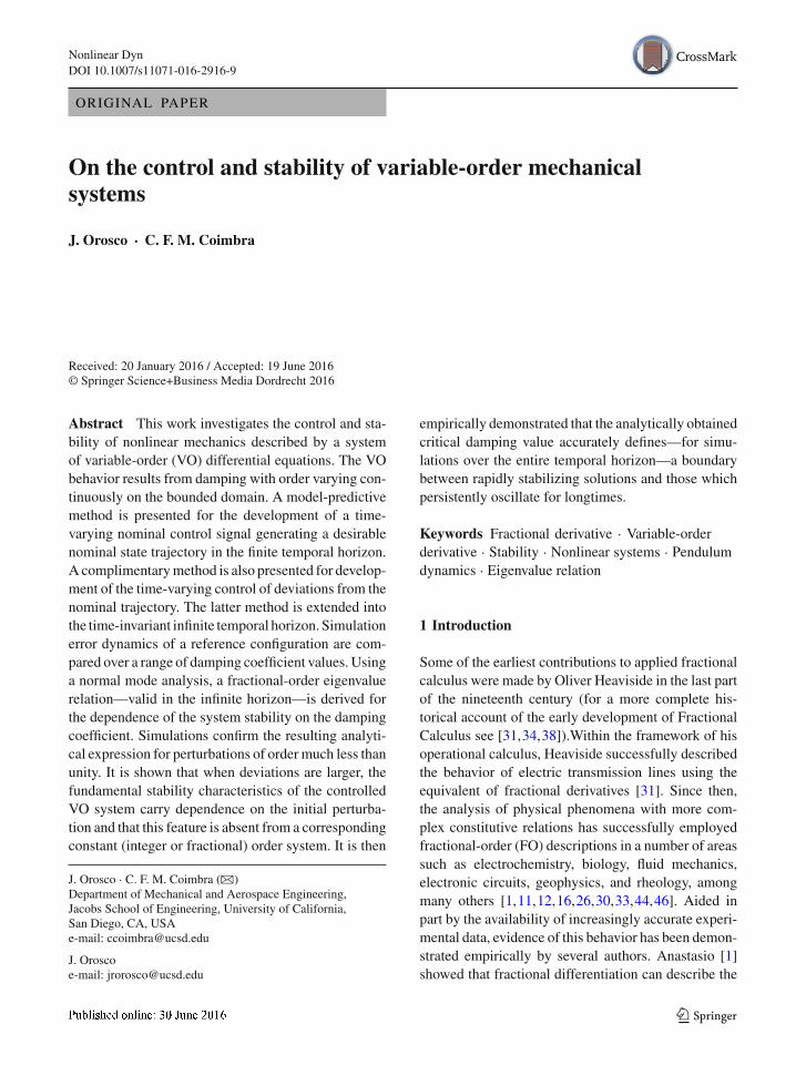
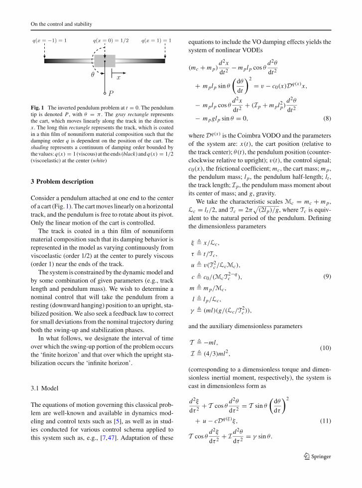
Fig. 1 The inverted pendulum problem at t = 0. The pendulumtip is denoted P , with θ = π . The gray rectangle representsthe cart, which moves linearly along the track in the directionx . The long thin rectangle represents the track, which is coatedin a thin film of nonuniform material composition such that thedamping order q is dependent on the position of the cart. Theshading represents a continuum of damping order bounded bythevalues:q(x) = 1 (viscous) at the ends (black) andq(x) = 1/2(viscoelastic) at the center (white)

3 Problem description

Consider a pendulum attached at one end to the centerof a cart (Fig. 1). The cartmoves linearly on a horizontaltrack, and the pendulum is free to rotate about its pivot.Only the linear motion of the cart is controlled.

The track is coated in a thin film of nonuniformmaterial composition such that its damping behavior isrepresented in the model as varying continuously fromviscoelastic (order 1/2) at the center to purely viscous(order 1) near the ends of the track.

The system is constrained by the dynamicmodel andby some combination of given parameters (e.g., tracklength and pendulum mass). We wish to determine anominal control that will take the pendulum from aresting (downward hanging) position to an upright, sta-bilized position.We also seek a feedback law to correctfor small deviations from the nominal trajectory duringboth the swing-up and stabilization phases.

In what follows, we designate the interval of timeover which the swing-up portion of the problem occursthe ‘finite horizon’ and that over which the upright sta-bilization occurs the ‘infinite horizon’.

3.1 Model

The equations of motion governing this classical prob-lem are well-known and available in dynamics mod-eling and control texts such as [5], as well as in stud-ies conducted for various control schema applied tothis system such as, e.g., [7,47]. Adaptation of these

equations to include the VO damping effects yields thesystem of nonlinear VODEs

(mc + mp)d2x

dt2− mplp cos θ

d2θ

dt2

+ mplp sin θ

(dθ

dt

)2

= v − c0(x)Dq(x)x,

− mplp cos θd2x

dt2+ (Ip + mpl

2p)d2θ

dt2

− mpglp sin θ = 0, (8)

whereDq(x) is the Coimbra VODO and the parametersof the system are: x(t), the cart position (relative tothe track center); θ(t), the pendulum position (counter-clockwise relative to upright); v(t), the control signal;c0(x), the frictional coefficient; mc, the cart mass; mp,the pendulum mass; l p, the pendulum half-length; lt ,the track length; Ip, the pendulummass moment aboutits center of mass; and g, gravity.

We take the characteristic scales Mc = mc + mp,Lc = lt/2, and Tc = 2π

√(2l p)/g, where Tc is equiv-

alent to the natural period of the pendulum. Definingthe dimensionless parameters

ξ � x/Lc,

τ � t/Tc,

u � v(T2c/LcMc),

c � c0/(McT2−qc ),

m � mp/Mc,

l � l p/Lc,

γ � (ml)(g/(Lc/T2c )),

(9)

and the auxiliary dimensionless parameters

T � −ml,

I � (4/3)ml2,(10)

(corresponding to a dimensionless torque and dimen-sionless inertial moment, respectively), the system iscast in dimensionless form as

d2ξ

dτ 2+ T cos θ

d2θ

dτ 2= T sin θ

(dθ

dτ

)2

+ u − cDq(ξ)ξ, (11)

T cos θd2ξ

dτ 2+ I d

2θ

dτ 2= γ sin θ.

123

J. Orosco, C. F. M. Coimbra

We consider a quadratic distribution of the VO fric-tional effects given by q(ξ(t)) = (1+ ξ(t)2)/2, so thatthe variable derivative order is always less than unityon the bounded domain. We will also take c constantfor the present analysis, noting that, in general, c maybe a function of the cart position. Finally, the temporalboundary distinguishing the finite and infinite horizonsis henceforth denoted τ = T .

4 Methods

In order to develop control solutions, the model isquasilinearized, leaving the VO term in nonlinearform. The nominal control and nominal trajectory aredevelopedusing an adjoint-basedminimizationmethodwith a combination of the linear and nonlinear modeldynamics. Optimal control of deviations from the nom-inal trajectory is then formulated from the linearizedportion of the quasilinearized system, regarding theVOdamping term as a nonlinear state disturbance.

The two proposed methods (one for time-invariantsystems and one for time-varying systems) are anextension of existing (well-established and fairly ubiq-uitous) methods for the control of constant integer-order differential equations. The general nonlinearform of the state-space equation given in the section tofollow can be used to model a broad class of problemsdefined by smooth VODEs. This includes ordinary dif-ferential equation discretizations of partial differentialsystems [5]. This is to say that themethods are indepen-dent of the pendulum problem, which is used here onlyto demonstrate the utility of the proposed methods.

As the entirety of the underlying mathematics forsuch a method can be found in many graduate levelcontrols texts, and the purpose of thiswork is to demon-strate the assimilation of VO dynamics and controlinto an existing (and well-documented) mathematicalframework, we provide here a concise summary ofthesemathematics as applied to the systemunder inves-tigation.

4.1 Quasilinearized state-space model

Defining the dimensionless state vector

ξ �(

ξ θdξ

dτ

dθ

dτ

)�, (12)

we can express Eq. (11) in the state-space form

ED1ξ = N (ξ , u) + FDqξ, (13)

which has the quasilinearization

ED1ξ = Aξ + Bu + FDqξ, (14)

where the matrices E and N are easily obtained byinspection (see, e.g., [5]), the matrices A and B areobtained as a linearization of N about some nominal ξand u, the matrix E = E(ξ), and F = [0 0 −c 0]�.

The state-space representation in Eq. (14) is a qua-silinear VO differential (in fact, integrodifferential)equation. Sufficient conditions for local controllabil-ity of equations of this type in Banach spaces havebeen described in [4]. The term FDqξ is bounded,and the linear control of quasilinear systems subject tobounded nonlinear state-dependent perturbations hasbeen recently studied [8,9,43]. We thus proceed withthe development of a linear control schema, treating thefrictional term as a bounded nonlinear state-dependentdisturbance.

4.2 Model-predictive control

We define the quadratic cost function

J (u) � 1

2

∫ T

0(ξ�Qξ + u�Ru)dτ

+ 1

2(Eξ)�QT Eξ , (15)

with Q ≥ 0, R > 0, and QT ≥ 0 being penalty(weighting) matrices used to tune the control responsefor the state trajectory, control effort, and terminal state,respectively. Since this method is an iterative descentmethod, the requirement for the R matrix is relaxed toR ≥ 0. For the optimal control methods that follow(which require the invertibility of R) the strict condi-tion holds. The terminal penalty matrix is, in particular,useful in the determination of an appropriate nominalcontrol during the model-predictive process, since thefinite-horizon control solution must ‘hand over’ a finalstate at τ = T that is tractable for the infinite-horizoncontrol solution on the interval τ ≥ T . By consideringsmall perturbations, u′, to the control input that resultin small perturbations, ξ ′, to the system trajectory, and

123

On the control and stability

developing the perturbation and adjoint equations, it isreadily shown that (cf. [5]) the gradient, g, of J withrespect to u—and constrained by the undisturbed sys-tem dynamics in Eq. (14)—is given by

g = B�r + Ru, (16)

where r is the costate, and its terminal condition isgiven by r(T ) = QT Eξ(T ). The costate adheres tothe dynamics described by the adjoint equations, whichare developed using the linearized portion of the systemdynamics. The adjoint equations are dependent on ξ ,so that in order to determine the gradient, one mustfirst obtain the state trajectory using the full nonlineardynamics. Accordingly, generation and optimizationof the nominal control and nominal state trajectory areachieved as follows:

1. guess an initial value for the control on τ ε [0, T ]and step the state forward through the interval usingthe full nonlinear dynamics of Eq. (13);

2. using the terminal condition on r , step the adjointsystem backward from τ = T using the linearizedadjoint equations developed from the linear por-tion of the quasilinearized dynamics described byEq. (14);

3. compute the gradient and update the control usingan appropriate conjugate gradient method;

4. iterate until some convergence criteria is met (oruntil a desirable nominal trajectory is obtained);and

5. store the resulting nominal control and state trajec-tory, denoted un and ξn, respectively.

4.3 Optimal control

Subsequent to the development of themodel-predictivecontrol signal, it is necessary to derive a feedback law tobe applied to errors between the nominal trajectory andthe actual trajectory. Letting ξ p(τ ) � ξ(τ )−ξn(τ ) andup(τ ) � u(τ ) − un(τ ) be the state and control errors,respectively, we define the quadratic cost function

J (up) � 1

2

∫ T

0(ξ p

�Qξ p+ up�Rup)dτ

+ 1

2(Eξ p)

�QT Eξ p, (17)

which is a functional on the error energy of the con-trolled system that includes a penalty on the terminalstate error. Following the same procedure outlined inSect. 4.2 to develop the gradient, we now use a directmethod. Setting the gradient equal to zero, we maywrite [5]

up = K ξ p, (18)

where

K = −R−1B�XE (19)

is the optimal feedback gain matrix and the determi-nation of X is achieved by solving the appropriatematrix Riccati equation in the finite or infinite horizonas needed.

4.3.1 Finite horizon

In the finite horizon, X = X (τ ) is the solution to thedifferential Riccati equation

dX

dτ= −( A�X + X A − XBR−1B�X + Q), (20)

where A � AE−1, Q � E−�QE−1, and both A andE are time-varying. The total control solution for τ ε

[0, T ] is then given by

u(τ ) = un(τ ) + up(τ ),

= un(τ ) + K f (τ )ξ p(τ ),(21)

with K f being the time-varying optimal feedback gainmatrix on the finite horizon, determined as in Eq. (19).

4.3.2 Infinite horizon

In the infinite horizon, the solution, X = X (τ ), canbe obtained by solving the differential Riccati equationfor τ → ∞. This is equivalently the constant solution,X , to the algebraic Riccati equation

0 = A�X E + E�X A − E�XBR−1B�, (22)

where A and E are now time invariant. The nominaltrajectory is identically null for τ ≥ T , so that un ≡0 ∀ τ ε [T,∞) and the resulting control solution is

123

J. Orosco, C. F. M. Coimbra

u(τ ) = up(τ ),

= Kiξ p(τ ),(23)

with Ki being the time-invariant optimal feedback gainmatrix on the infinite horizon, determined as inEq. (19).

5 Simulations

In light of the large number of parameters available fortuning the controller, it is desirable to define abasic con-figuration that is in some sense robust to the variationin the frictional coefficient. We choose the followingfor the physical parameters of the system: g = 9.81,lt = 2, mc = 1, mp = 0.05, and l p = 0.15. The unitsare SI. Parameters for the simulation were selected toreflect realistic conditions given the nature of the prob-lem. For the temporal discretization, the numerical stepsize h = 0.01 was used. We let the boundary betweenthe finite and infinite horizons be τ = T = 2. Whenτ = T , the nominal trajectory resulting from the pen-dulum swing-up is not the state-space origin, so thatthe upright stabilization phase is automatically subjectto an initial perturbation requiring control correctionsin the infinite horizon. Regardless, we introduce a per-turbation to the initial state given by

ξ(0) =

⎛⎜⎜⎝

−0.1π − 0.1

00

⎞⎟⎟⎠ , (24)

so that the efficacy of the time-varying error correct-ing control signal over the finite horizon may also beobserved. Finally, we take the basic tuning configu-ration Q = diag(0, 0, 0, 0), R = 0, and QT =diag(20, 12, 0.1, 20, 000) for generation of the nom-inal control using the model-predictive methods ofSect. 4.2. Doing so yields a state at τ = T which isstable to a range of frictional values when all subse-quent tuningparameters set to unity or the appropriatelysized identity matrix. That is, by a judicious choice ofthe parameters used to develop the nominal trajectory,the control solution for the error dynamics can then bedeveloped as though there is no weighting applied tothe states or to the control in the cost functional, so thatthe feedback law is everywhere a result of a direct mea-sure of the systemic error energy. In the analysis to fol-low, no effort is made to tune the controller beyond the

basic defined configuration. This provides a referencefor comparison of the system dynamics over the inves-tigated frictional values. With the system configured asdescribed, the method produces a stabilizing solutionon the bounded domain for c ε [0, 1.89]. Simulationswere conducted on this interval with a frictional stepsize Δc = 0.01.

5.1 Controlled dynamics

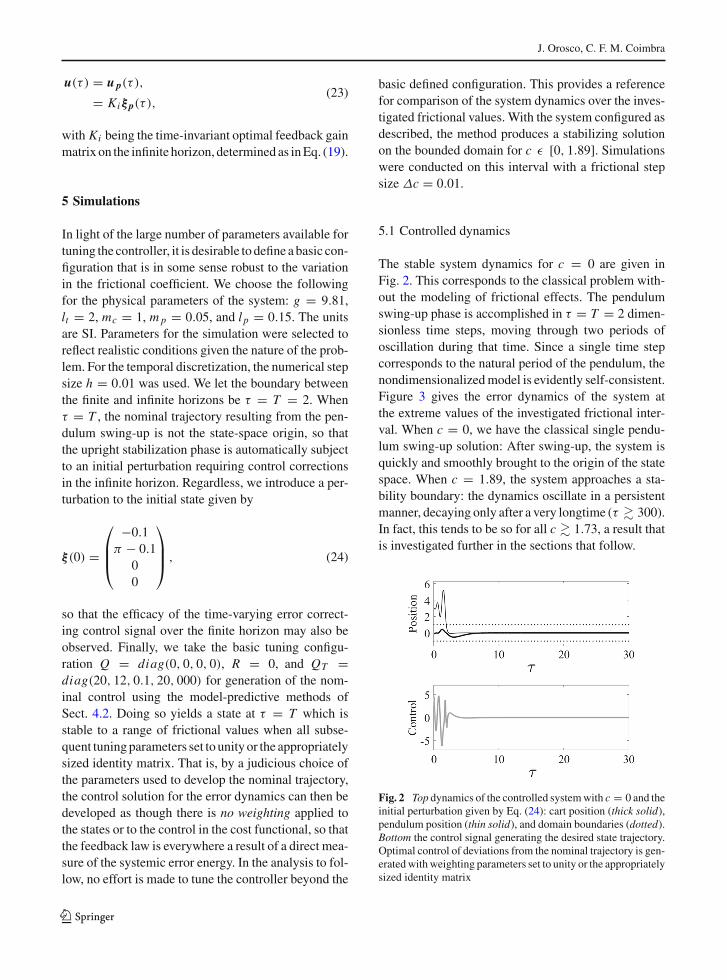
The stable system dynamics for c = 0 are given inFig. 2. This corresponds to the classical problem with-out the modeling of frictional effects. The pendulumswing-up phase is accomplished in τ = T = 2 dimen-sionless time steps, moving through two periods ofoscillation during that time. Since a single time stepcorresponds to the natural period of the pendulum, thenondimensionalizedmodel is evidently self-consistent.Figure 3 gives the error dynamics of the system atthe extreme values of the investigated frictional inter-val. When c = 0, we have the classical single pendu-lum swing-up solution: After swing-up, the system isquickly and smoothly brought to the origin of the statespace. When c = 1.89, the system approaches a sta-bility boundary: the dynamics oscillate in a persistentmanner, decaying only after a very longtime (τ � 300).In fact, this tends to be so for all c � 1.73, a result thatis investigated further in the sections that follow.

Fig. 2 Top dynamics of the controlled systemwith c = 0 and theinitial perturbation given by Eq. (24): cart position (thick solid),pendulum position (thin solid), and domain boundaries (dotted).Bottom the control signal generating the desired state trajectory.Optimal control of deviations from the nominal trajectory is gen-eratedwithweighting parameters set to unity or the appropriatelysized identity matrix

123

On the control and stability

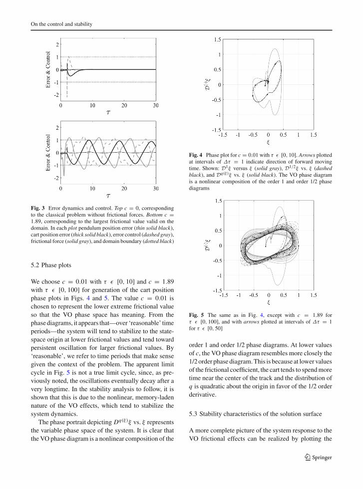
Fig. 3 Error dynamics and control. Top c = 0, correspondingto the classical problem without frictional forces. Bottom c =1.89, corresponding to the largest frictional value valid on thedomain. In each plot pendulum position error (thin solid black),cart position error (thick solid black), error control (dashed gray),frictional force (solid gray), and domain boundary (dotted black)

5.2 Phase plots

We choose c = 0.01 with τ ε [0, 10] and c = 1.89with τ ε [0, 100] for generation of the cart positionphase plots in Figs. 4 and 5. The value c = 0.01 ischosen to represent the lower extreme frictional valueso that the VO phase space has meaning. From thephase diagrams, it appears that—over ‘reasonable’ timeperiods—the system will tend to stabilize to the state-space origin at lower frictional values and tend towardpersistent oscillation for larger frictional values. By‘reasonable’, we refer to time periods that make sensegiven the context of the problem. The apparent limitcycle in Fig. 5 is not a true limit cycle, since, as pre-viously noted, the oscillations eventually decay after avery longtime. In the stability analysis to follow, it isshown that this is due to the nonlinear, memory-ladennature of the VO effects, which tend to stabilize thesystem dynamics.

The phase portrait depicting Dq(ξ)ξ vs. ξ representsthe variable phase space of the system. It is clear thatthe VO phase diagram is a nonlinear composition of the

Fig. 4 Phase plot for c = 0.01 with τ ε [0, 10]. Arrows plottedat intervals of Δτ = 1 indicate direction of forward movingtime. Shown: D1ξ versus ξ (solid gray), D1/2ξ vs. ξ (dashedblack), and Dq(ξ)ξ vs. ξ (solid black). The VO phase diagramis a nonlinear composition of the order 1 and order 1/2 phasediagrams

Fig. 5 The same as in Fig. 4, except with c = 1.89 forτ ε [0, 100], and with arrows plotted at intervals of Δτ = 1for τ ε [0, 50]

order 1 and order 1/2 phase diagrams. At lower valuesof c, the VO phase diagram resembles more closely the1/2 order phase diagram.This is because at lower valuesof the frictional coefficient, the cart tends to spendmoretime near the center of the track and the distribution ofq is quadratic about the origin in favor of the 1/2 orderderivative.

5.3 Stability characteristics of the solution surface

A more complete picture of the system response to theVO frictional effects can be realized by plotting the

123

J. Orosco, C. F. M. Coimbra

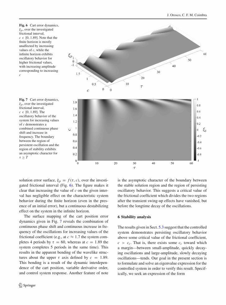
Fig. 6 Cart error dynamics,ξp , over the investigatedfrictional interval,c ε [0, 1.89]. Note that thefinite horizon is mostlyunaffected by increasingvalues of c, while theinfinite horizon exhibitsoscillatory behavior forhigher frictional values,with increasing amplitudecorresponding to increasingc

Fig. 7 Cart error dynamics,ξp , over the investigatedfrictional interval,c ε [0, 1.89]. Theoscillatory behavior of thesystem for increasing valuesof c demonstrates acombined continuous phaseshift and increase infrequency. The boundarybetween the region ofpersistent oscillation and theregion of stability exhibitsan asymptotic character forτ ≥ T

solution error surface, ξp = f (τ, c), over the investi-gated frictional interval (Fig. 6). The figure makes itclear that increasing the value of c on the given inter-val has negligible effect on the characteristic systembehavior during the finite horizon (even in the pres-ence of an initial error), but a continuous destabilizingeffect on the system in the infinite horizon.

The surface mapping of the cart position errordynamics given in Fig. 7 reveals the combination ofcontinuous phase shift and continuous increase in fre-quency of the oscillations for increasing values of thefrictional coefficient (e.g., at c ≈ 1.7 the system com-pletes 4 periods by τ = 60, whereas at c = 1.89 thesystem completes 5 periods in the same time). Thisresults in the apparent bending of the wavelike struc-tures about the upper τ axis defined by c = 1.89.This bending is a result of the dynamic interdepen-dence of the cart position, variable derivative order,and control system response. Another feature of note

is the asymptotic character of the boundary betweenthe stable solution region and the region of persistingoscillatory behavior. This suggests a critical value ofthe frictional coefficient which divides the two regionsafter the transient swing-up effects have vanished, butbefore the longtime decay of the oscillations.

6 Stability analysis

The results given in Sect. 5.3 suggest that the controlledsystem demonstrates persisting oscillatory behaviorabove some critical value of the frictional coefficient,c > cc. That is, there exists some cc toward whicha margin—between small-amplitude, quickly decay-ing oscillations and large-amplitude, slowly decayingoscillations—tends. Our goal in the present section isto formulate and solve an eigenvalue expression for thecontrolled system in order to verify this result. Specif-ically, we seek an expression of the form

123

On the control and stability

F(s; c) = 0, (25)

where s ε C denotes an eigenvalue of the system. If welet sc correspond to the most unstable mode, then [20]:if Re(sc) < 0, the system is said to be asymptoticallystable; if Re(sc) > 0, the system is said to be unstable;and if Re(sc) ≡ 0, the system is said to be neutrallystable. We employ a linear stability analysis typical of,e.g., fluid mechanical systems and delineated in stan-dard hydrodynamic stability texts such as [20].We takeour analysis on the infinite horizon and define—in thelanguage of hydrodynamic stability—our ‘basic’ solu-tion, denoted here ξ , to be the nominal trajectory (whichin the infinite horizon is the origin of the state-space).The basic trajectory is generated by the basic control(i.e., the nominal control), denoted here u = 0.

6.1 Developing the eigenvalue relation, F(s; c) = 0

We define the perturbed state

ξ � ξ + ξ ′,= ξ ′,

=(

ξ ′ θ ′ dξ ′

dτ

dθ ′

dτ

)�,

(26)

and the perturbed control

u � u + u′,= u′,

(27)

where the primed quantities are taken to be much lessthan unity. Substituting the perturbed quantities intoEq. (11), subtracting the nominal solution, and notingthat nonlinear primed terms are negligible comparedto the other terms (e.g., θ ′ξ ′ ≈ 0), we arrive at theperturbation equations

d2ξ ′

dτ 2+ T d2θ ′

v2= u′ − cD1/2ξ ′,

T d2ξ ′

dτ 2+ I d

2θ ′

dτ 2= γ θ ′.

(28)

That the VODO reduces to a constant half-order oper-ator when linearized about the nominal trajectory willbecome important in a later analysis of the simulationresults. The perturbation control signal is a feedback on

the state perturbation, with the optimal feedback gainmatrix being K = (kξ kθ kD1ξ kD1θ ), so that

u′ = K ξ ′,

= kξ ξ′ + kθ θ

′ + kD1ξ

dξ ′

dτ+ kD1θ

dθ ′

dτ.

(29)

Proceeding with a normal mode analysis, we define ournormal modes to be

ξ ′ � ξesτ ,

θ ′ � θesτ ,(30)

where ξ and θ are functions of the ξ -coordinate alone.Then,

D1/2ξ ′ = D1/2ξesτ ,

= [esτ√sEr f (√sτ)]ξ ,

(31)

where Er f (·) denotes the error function, and wherewe have chosen the Caputo definition for evaluationof the semiderivative. The Caputo definition results inan expression that is valid for τ = 0, whereas other,less restrictive operators (e.g., Riemann-Liouville andGrünwald-Letnikov) result in an expression with sin-gular behavior near τ = 0. For large τ—that is, in theinfinite horizon—Eq. (31) becomes

limτ→∞D1/2ξ ′ = s1/2ξ ′. (32)

Substituting Eqs. (29), (30), and (32) into Eq. (28) anddividing out exponential terms, we have

s2ξ + T s2θ = kξ ξ + kθ θ

+ kD1ξ sξ + kD1θ sθ − cs1/2ξ ,

T s2ξ + Is2θ = γ θ . (33)

Solving the bottom equation for θ , substituting into thetop equation, and then dividing through by ξ yield thedesired eigenvalue relation, F(s; c) = 0, given by theexpression

(I − T 2)s4 + (T kD1θ − IkD1ξ )s3 + (Ic)s5/2

+ (T kθ − Ikξ − γ )s2 + (γ kD1θ )s

− (γ c)s1/2 + γ kξ = 0, (34)

123

J. Orosco, C. F. M. Coimbra

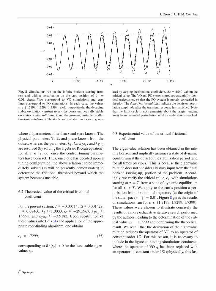
Fig. 8 Simulations run on the infinite horizon starting fromrest and with a perturbation on the cart position of ξ ′ =0.01. Black lines correspond to VO simulations and graylines correspond to FO simulations. In each case, the valuesc ε {1.7199, 1.7299, 1.7399} yield, respectively, the decayingstable oscillation (dashed lines), the persistent neutrally stableoscillation (thick solid lines), and the growing unstable oscilla-tion (thin solid lines). The stable and unstable modes were gener-

ated by varying the frictional coefficient,Δc = ±0.01, about thecritical value. The VO and FO systems produce essentially iden-tical trajectories, so that the FO system is mostly concealed inthe plot. The dotted horizontal lines indicate the persistent oscil-lation amplitude after the transient response has vanished. Notethat the limit cycle is not symmetric about the origin, tendingaway from the initial perturbation until a steady state is reached

where all parameters other than s and c are known. Thephysical parameters T , I, and γ are known from theoutset, whereas the parameters kξ , kθ , kD1ξ , and kD1θ

are resolved (by solving the algebraic Riccati equation)for all τ ε [T,∞) once the control tuning parame-ters have been set. Thus, once one has decided upon atuning configuration, the above relation can be imme-diately solved (as will be presently demonstrated) todetermine the frictional threshold beyond which thesystem becomes unstable.

6.2 Theoretical value of the critical frictionalcoefficient

For the present system, T ≈−0.007143, I≈0.001429,γ ≈ 0.08460, kξ ≈ 1.0000, kθ ≈ −29.5967, kD1ξ ≈1.9995, and kD1θ ≈ −3.9182. Upon substitution ofthese values into Eq. (34) and application of the appro-priate root-finding algorithm, one obtains

cc ≈ 1.7299, (35)

corresponding to Re(sc) ≈ 0 for the least stable eigen-value, sc.

6.3 Experimental value of the critical frictionalcoefficient

The eigenvalue relation has been obtained in the infi-nite horizon and implicitly assumes a state of dynamicequilibrium at the outset of the stabilization period (andfor all times previous). This is because the eigenvaluerelation does not consider a history input from the finitehorizon (swing-up) portion of the problem. Accord-ingly, we verify the critical value, cc, with simulationsstarting at τ = T from a state of dynamic equilibriumfor all τ < T . We apply to the cart’s position a per-turbation from the nominal trajectory (at the origin ofthe state-space) of ξ ′ = 0.01. Figure 8 gives the resultsof simulations run for c ε {1.7199, 1.7299, 1.7399}.These values were chosen to illustrate concisely theresults of a more exhaustive iterative search performedby the authors, leading to the determination of the crit-ical value cc = 1.7299 and confirming the theoreticalresult. We recall that the derivation of the eigenvaluerelation reduces the operator of VO to an operator ofconstant-order 1/2. For this reason, it is necessary toinclude in the figure coinciding simulations conductedwhere the operator of VO q has been replaced withan operator of constant-order 1/2 (physically, this last

123

On the control and stability

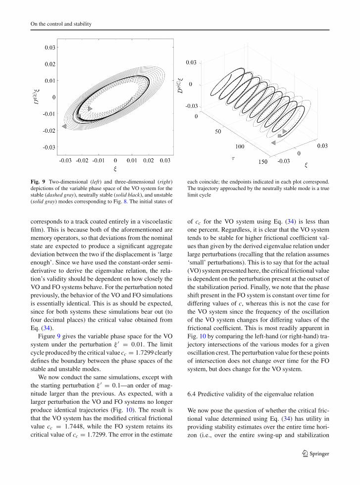
Fig. 9 Two-dimensional (left) and three-dimensional (right)depictions of the variable phase space of the VO system for thestable (dashed gray), neutrally stable (solid black), and unstable(solid gray) modes corresponding to Fig. 8. The initial states of

each coincide; the endpoints indicated in each plot correspond.The trajectory approached by the neutrally stable mode is a truelimit cycle

corresponds to a track coated entirely in a viscoelasticfilm). This is because both of the aforementioned arememory operators, so that deviations from the nominalstate are expected to produce a significant aggregatedeviation between the two if the displacement is ‘largeenough’. Since we have used the constant-order semi-derivative to derive the eigenvalue relation, the rela-tion’s validity should be dependent on how closely theVO and FO systems behave. For the perturbation notedpreviously, the behavior of the VO and FO simulationsis essentially identical. This is as should be expected,since for both systems these simulations bear out (tofour decimal places) the critical value obtained fromEq. (34).

Figure 9 gives the variable phase space for the VOsystem under the perturbation ξ ′ = 0.01. The limitcycle producedby the critical value cc = 1.7299clearlydefines the boundary between the phase spaces of thestable and unstable modes.

We now conduct the same simulations, except withthe starting perturbation ξ ′ = 0.1—an order of mag-nitude larger than the previous. As expected, with alarger perturbation the VO and FO systems no longerproduce identical trajectories (Fig. 10). The result isthat the VO system has the modified critical frictionalvalue cc = 1.7448, while the FO system retains itscritical value of cc = 1.7299. The error in the estimate

of cc for the VO system using Eq. (34) is less thanone percent. Regardless, it is clear that the VO systemtends to be stable for higher frictional coefficient val-ues than given by the derived eigenvalue relation underlarge perturbations (recalling that the relation assumes‘small’ perturbations). This is to say that for the actual(VO) system presented here, the critical frictional valueis dependent on the perturbation present at the outset ofthe stabilization period. Finally, we note that the phaseshift present in the FO system is constant over time fordiffering values of c, whereas this is not the case forthe VO system since the frequency of the oscillationof the VO system changes for differing values of thefrictional coefficient. This is most readily apparent inFig. 10 by comparing the left-hand (or right-hand) tra-jectory intersections of the various modes for a givenoscillation crest. The perturbation value for these pointsof intersection does not change over time for the FOsystem, but does change for the VO system.

6.4 Predictive validity of the eigenvalue relation

We now pose the question of whether the critical fric-tional value determined using Eq. (34) has utility inproviding stability estimates over the entire time hori-zon (i.e., over the entire swing-up and stabilization

123

J. Orosco, C. F. M. Coimbra

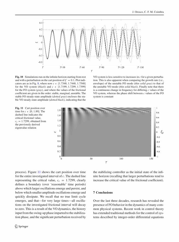
Fig. 10 Simulations run on the infinite horizon starting from restandwith a perturbation on the cart position of ξ ′ = 0.1. Plot indi-cators are as in Fig. 8, where now c ε {1.7348, 1.7448, 1.7548}for the VO system (black) and c ε {1.7199, 1.7299, 1.7399}for the FO system (gray), and where the values of the frictionalcoefficient are given in the order: stable, marginal, unstable. Thestable FO steady-state amplitude (dotted gray) encloses the sta-ble VO steady-state amplitude (dotted black), indicating that the

VO system is less sensitive to increases in c for a given perturba-tion. This is also apparent when comparing the growth rate (i.e.,envelope) of the unstable FO mode (thin solid gray) to that ofthe unstable VO mode (thin solid black). Finally note that thereis a continuous change in frequency for differing c values of theVO system, whereas the phase shift between c values of the FOsystem is constant

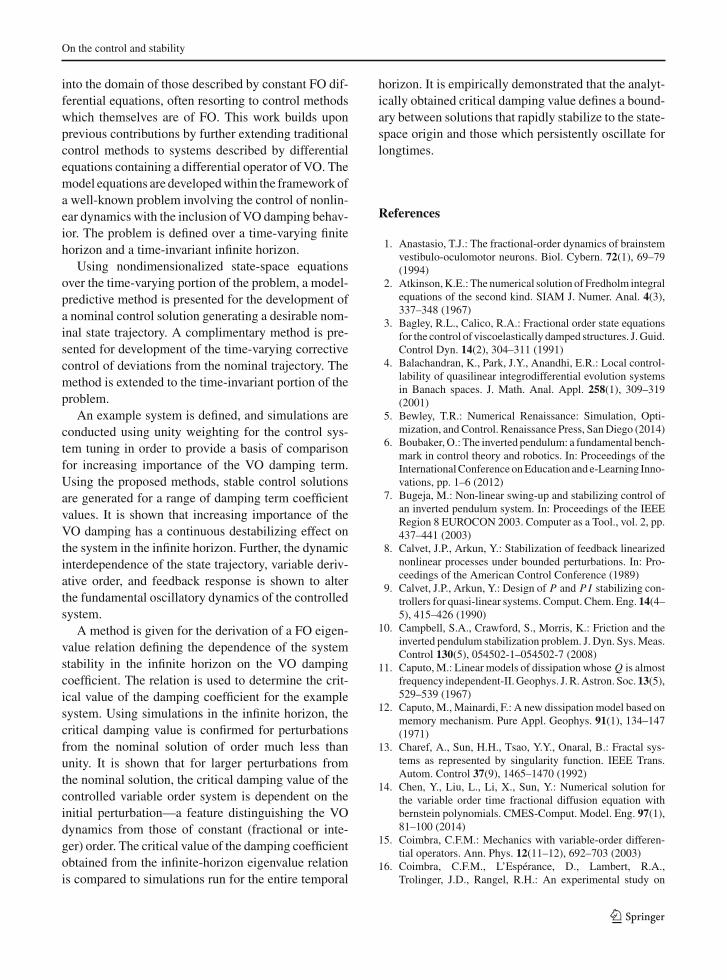
Fig. 11 Cart position overtime for c ε [0, 1.89]. Thedashed line indicates thecritical frictional value,cc = 1.7299, obtained fromthe previously derivedeigenvalue relation

process). Figure 11 shows the cart position over timefor the entire investigated interval of c. The dashed linerepresenting the critical value, cc = 1.7299, clearlydefines a boundary (over ‘reasonable’ time periods)above which larger oscillations emerge and persist, andbelowwhich smaller amplitude oscillations emerge andquickly dissipate. We recall that no true limit cycleemerges, and that—for very large times—all oscilla-tions on the investigated frictional interval will decayto zero. This is a result of the VO dynamics, the historyinput from the swing-up phase imparted to the stabiliza-tion phase, and the significant perturbation received by

the stabilizing controller as the initial state of the infi-nite horizon (recalling that larger perturbations tend toincrease the critical value of the frictional coefficient).

7 Conclusions

Over the last three decades, research has revealed thepresence of FO behavior in the dynamics of many com-mon physical systems. Recent work in control theoryhas extended traditional methods for the control of sys-tems described by integer-order differential equations

123

On the control and stability

into the domain of those described by constant FO dif-ferential equations, often resorting to control methodswhich themselves are of FO. This work builds uponprevious contributions by further extending traditionalcontrol methods to systems described by differentialequations containing a differential operator of VO. Themodel equations are developedwithin the framework ofa well-known problem involving the control of nonlin-ear dynamics with the inclusion of VO damping behav-ior. The problem is defined over a time-varying finitehorizon and a time-invariant infinite horizon.

Using nondimensionalized state-space equationsover the time-varying portion of the problem, a model-predictive method is presented for the development ofa nominal control solution generating a desirable nom-inal state trajectory. A complimentary method is pre-sented for development of the time-varying correctivecontrol of deviations from the nominal trajectory. Themethod is extended to the time-invariant portion of theproblem.

An example system is defined, and simulations areconducted using unity weighting for the control sys-tem tuning in order to provide a basis of comparisonfor increasing importance of the VO damping term.Using the proposed methods, stable control solutionsare generated for a range of damping term coefficientvalues. It is shown that increasing importance of theVO damping has a continuous destabilizing effect onthe system in the infinite horizon. Further, the dynamicinterdependence of the state trajectory, variable deriv-ative order, and feedback response is shown to alterthe fundamental oscillatory dynamics of the controlledsystem.

A method is given for the derivation of a FO eigen-value relation defining the dependence of the systemstability in the infinite horizon on the VO dampingcoefficient. The relation is used to determine the crit-ical value of the damping coefficient for the examplesystem. Using simulations in the infinite horizon, thecritical damping value is confirmed for perturbationsfrom the nominal solution of order much less thanunity. It is shown that for larger perturbations fromthe nominal solution, the critical damping value of thecontrolled variable order system is dependent on theinitial perturbation—a feature distinguishing the VOdynamics from those of constant (fractional or inte-ger) order. The critical value of the damping coefficientobtained from the infinite-horizon eigenvalue relationis compared to simulations run for the entire temporal

horizon. It is empirically demonstrated that the analyt-ically obtained critical damping value defines a bound-ary between solutions that rapidly stabilize to the state-space origin and those which persistently oscillate forlongtimes.

References

1. Anastasio, T.J.: The fractional-order dynamics of brainstemvestibulo-oculomotor neurons. Biol. Cybern. 72(1), 69–79(1994)

2. Atkinson,K.E.: The numerical solution of Fredholm integralequations of the second kind. SIAM J. Numer. Anal. 4(3),337–348 (1967)

3. Bagley, R.L., Calico, R.A.: Fractional order state equationsfor the control of viscoelastically damped structures. J.Guid.Control Dyn. 14(2), 304–311 (1991)

4. Balachandran, K., Park, J.Y., Anandhi, E.R.: Local control-lability of quasilinear integrodifferential evolution systemsin Banach spaces. J. Math. Anal. Appl. 258(1), 309–319(2001)

5. Bewley, T.R.: Numerical Renaissance: Simulation, Opti-mization, and Control. Renaissance Press, SanDiego (2014)

6. Boubaker,O.: The inverted pendulum: a fundamental bench-mark in control theory and robotics. In: Proceedings of theInternationalConference onEducation and e-Learning Inno-vations, pp. 1–6 (2012)

7. Bugeja, M.: Non-linear swing-up and stabilizing control ofan inverted pendulum system. In: Proceedings of the IEEERegion 8 EUROCON 2003. Computer as a Tool., vol. 2, pp.437–441 (2003)

8. Calvet, J.P., Arkun, Y.: Stabilization of feedback linearizednonlinear processes under bounded perturbations. In: Pro-ceedings of the American Control Conference (1989)

9. Calvet, J.P., Arkun, Y.: Design of P and P I stabilizing con-trollers for quasi-linear systems. Comput. Chem. Eng. 14(4–5), 415–426 (1990)

10. Campbell, S.A., Crawford, S., Morris, K.: Friction and theinverted pendulum stabilization problem. J. Dyn. Sys.Meas.Control 130(5), 054502-1–054502-7 (2008)

11. Caputo, M.: Linear models of dissipation whose Q is almostfrequency independent-II.Geophys. J.R.Astron. Soc.13(5),529–539 (1967)

12. Caputo, M., Mainardi, F.: A new dissipation model based onmemory mechanism. Pure Appl. Geophys. 91(1), 134–147(1971)

13. Charef, A., Sun, H.H., Tsao, Y.Y., Onaral, B.: Fractal sys-tems as represented by singularity function. IEEE Trans.Autom. Control 37(9), 1465–1470 (1992)

14. Chen, Y., Liu, L., Li, X., Sun, Y.: Numerical solution forthe variable order time fractional diffusion equation withbernstein polynomials. CMES-Comput. Model. Eng. 97(1),81–100 (2014)

15. Coimbra, C.F.M.: Mechanics with variable-order differen-tial operators. Ann. Phys. 12(11–12), 692–703 (2003)

16. Coimbra, C.F.M., L’Espérance, D., Lambert, R.A.,Trolinger, J.D., Rangel, R.H.: An experimental study on

123

J. Orosco, C. F. M. Coimbra

stationary history effects in high-frequency Stokes flows.J. Fluid Mech. 504, 353–363 (2004)

17. Diaz, G., Coimbra, C.F.M.: Nonlinear dynamics and controlof a variable order oscillator with application to the van derPol equation. Nonlinear Dyn. 56(1–2), 145–157 (2009)

18. Diaz, G., Coimbra, C.F.M.: Dynamics and control of non-linear variable order oscillators. In: Evans, T. (ed.) Non-linear Dynamics, Chapter 6, pp. 129–144. InTech, Rijeka(2010)

19. Drazin, P.G.: Nonlinear Systems, 2nd edn. Cambridge Uni-versity Press, Cambridge (1992)

20. Drazin, P.G., Reid, W.H.: Hydrodynamic Stability, 2nd edn.Cambridge University Press, Cambridge (2004)

21. Durand, S., Guerrero-Castellanos, J.F., Marchand, N.,Guerrero-Sánchez,W.F.: Event-based control of the invertedpendulum: swing up and stabilization. J. Control Eng. Appl.Inform. 15(3), 96–104 (2013)

22. Hartley, T.T., Lorenzo, C.F.: Dynamics and control of initial-ized fractional-order systems. Nonlinear Dyn. 29(1), 201–233 (2002)

23. Hwang,C., Leu, J.F., Tsay, S.Y.:Anote on time-domain sim-ulation of feedback fractional-order systems. IEEE Trans.Autom. Control 47(4), 625–631 (2002)

24. Ingman, D., Suzdalnitsky, J., Zeifman, M.: Constitutivedynamic-order model for nonlinear contact phenomena. J.Appl. Mech. 67(2), 383–390 (1999)

25. Khalil, H.K.: Nonlinear Systems, 3rd edn. Prentice Hall,Upper Saddle River (2002)

26. L’Espérance, D., Coimbra, C.F.M., Trolinger, J.D., Rangel,R.H.: Experimental verification of fractional history effectson the viscous dynamics of small spherical particles. Exp.Fluids 38(1), 112–116 (2005)

27. Li, Y., Chen, Y.: Fractional order linear quadratic regulator.In: Proceedings of the IEEE/ASME International Confer-ence on Mechatronic and Embedded Systems and Applica-tions, pp. 363–368 (2008)

28. Lorenzo, C.F., Hartley, T.T.: Initialization in fractional ordersystems. In: Proceedings of the European Control Confer-ence, pp. 1471–1476 (2001)

29. Lorenzo, C.F., Hartley, T.T.: Variable order and distributedorder fractional operators. Nonlinear Dyn. 29(1), 57–98(2002)

30. Mainardi, F.: Fractional Calculus and Waves in LinearViscoelasticity: An Introduction to Mathematical Models.Imperial College Press, London (2010)

31. Miller, K.S., Ross, B.: An Introduction to the FractionalCalculus and Fractional Differential Equations. Wiley, NewYork (1993)

32. Monje, C.A., Chen, Y., Vinagre, B.M., Xue, D., Feliu, V.:Fractional-Order Systems and Controls. Advances in Indus-trial Control. Springer, London (2010)

33. Oldham,K.B., Spanier, J.: The replacement of Fick’s lawsbya formulation involving semidifferentiation. J. Electroanal.Chem. Interfacial Electrochem. 26(2—-3), 331–341 (1970)

34. Oldham, K.B., Spanier, J.: The Fractional Calculus. Acad-emic Press, San Diego (1974)

35. Podlubny, I.: Fractional Differential Equations. AcademicPress, San Diego (1999)

36. Podlubny, I.: Fractional-order systems and P I λDμ-controllers. IEEE Trans. Autom. Control 44(1), 208–214(1999)

37. Ramirez, L.E.S., Coimbra, C.F.M.: On the selection andmeaning of variable order operators for dynamic modeling.Int. J. Differ. Equ. 2010, Article ID 846107 (2010)

38. Ross, B.: The development of fractional calculus 1695–1900. Hist. Math. 4(1), 75–89 (1977)

39. Ross, B., Samko, S.G.: Fractional integration operator ofvariable order in theHölder spaces Hλ(x). Int. J.Math.Math.Sci. 18(4), 777–788 (1995)

40. Samko, S.G., Ross, B.: Integration and differentiation to avariable fractional order. Integral Transforms Spec. Funct.1(4), 277–300 (1993)

41. Shen, S., Liu, F., Chen, J., Turner, I., Anh, V.: Numeri-cal techniques for the variable order time fractional diffu-sion equation. Appl. Math. Comput. 218(22), 10861–10870(2012)

42. Soon, C.M., Coimbra, C.F.M., Kobayashi, M.H.: The vari-able viscoelasticity oscillator. Ann. Phys. 14(6), 378–389(2005)

43. Sun, Z., Tsao, T.C.: Control of linear systems with nonlin-ear disturbance dynamics. In: Proceedings of the AmericanControl Conference, vol. 4, pp. 3049–3054 (2001)

44. Torvik, P.J.,Bagley,R.L.:On the appearanceof the fractionalderivative in the behavior of real materials. J. Appl. Mech.51(2), 294–298 (1984)

45. Wang, L., Ma, Y., Yang, Y.: Legendre polynomials methodfor solving a class of variable order fractional differen-tial equation. CMES-Comput. Model. Eng. 101(2), 97–111(2014)

46. Westerlund, S.: Dead matter has memory!. Phys. Scr. 43(2),174–179 (1991)

47. Yang, J.H., Shim, S.Y., Seo, J.H., Lee, Y.S.: Swing-up con-trol for an inverted pendulum with restricted cart rail length.Int. J. Control Autom. 7(4), 674–680 (2009)

48. Zhang, H., Liu, F., Zhuang, P., Turner, I., Anh, V.: Numer-ical analysis of a new space-time variable fractional orderadvection-dispersion equation. Appl. Math. Comput. 242,541–550 (2014)

49. Zhang,H., Shen, S.: The numerical simulation of space–timevariable fractional order diffusion equation. Numer. Math.Theor. Methods Appl. 6(4), 571–585 (2013)

123