ON THE CONTINUATION OF PERIODIC ORBITS* 1. Introduction

METHODS AND APPLICATIONS OF ANALYSIS. (C) 2000 International Press Vol. 7, No. 1, pp. 85-104, March 2000 005

ON THE CONTINUATION OF PERIODIC ORBITS*

M. B. H. RHOUMAt AND C. CHICONE*

Abstract. Using Poincare's method and a Lyapanov-Schmidt reduction, a continuation theorem for resonant periodic orbits of periodically forced oscillators is proved that does not require the unperturbed manifold of periodic solutions to be normally nondegenerate. This is accomplished with the aid of a generalization of the Poincare-Melnikov function that includes second derivatives and with the introduction of associated families of differential equations where the bifurcation parameter is a power of the original small parameter. Incidentally, a result of J. Cronin [Meth. Appl. Anal, Vol. 3 (1996), pp. 370-400] that inspired this work is corrected.

1. Introduction. Oscillations play a prominent role in many physical and bio- logical systems where an important problem is to determine if spontaneous oscillatory activity persists when subjected to a small external periodic stimulus. We will discuss some methods that can be used to solve this problem.

Consider the family of differential equations

(1.1) y = f(y) + eg(t,y,e)

where y € En, e > 0, and, for each fixed e > 0 and v E ln, the function t H> g(t, v, e) is periodic with period T > 0. We will assume that the unperturbed system

(1-2) V = /(»)

has a resonant period manifold Z C Rn, that is, Z is a manifold consisting entirely of To-periodic orbits where To > 0 and there is a pair of relatively prime positive integers M and N such that

(1.3) MTQ = NT.

The basic problem that we will address is the persistence of the periodic orbits in Z. In other words, we will study the existence of periodic orbits with period iVT for small e > 0.

Several authors, for example [1, 2, 3, 4, 11, 12, 13, 14, 17, 21], have treated the general persistence problem, albeit from different perspectives, and they have all obtained the same basic result under an assumption on the period manifold Z that we call normal nondegeneracy. This nondegeneracy assumption is expressible as a condition on the linearized unperturbed flow over Z. Indeed, for v E W1 let t h-» y(t,v,e) denote the solution of system (1.2) such that y(0,v,e) = v and let $(t,v) denote the principal fundamental matrix at time t = 0 of the first variational equation

(1.4) w = Df(y(t,v,0))w

Of course, in this case the principal fundamental matrix solution is just the partial derivative of the solution of the original unperturbed differential equation with respect to v, that is,

*(t,v) =yv(t,v,0).

* Revised on July 16, 1999. tCDSNS, Georgia Institute of Technology, Atlanta, GA 30332, USA ([email protected]). ^Department of Mathematics, University of Missouri, Columbia, MO 65211, USA (carmen

@chicone.math.missouri.edu).

85

86 M. RHOUMA AND C. CHICONE

The manifold Z is called normally nondegenerate if for each C G Z the dimension of the kernel /C(£) of the linear transformation $(iVT,C) — / (called the infinitesimal displacement) and the dimension of the manifold Z coincide.

A normally hyperbolic period manifold, for example a hyperbolic limit cycle, is normally nondegenerate, but normal hyperbolicity is not a necessary condition for normal nondegeneracy. For example, in case n = 2, a periodic orbit F in an annulus of periodic orbits is normally nondegenerate provided that the derivative of the period function with respect to a regular parameter on a transverse section E does not vanish at the point where F meets E.

The normal nondegeneracy property and the implicit function theorem are used to reduce the problem of the persistence of resonant unperturbed periodic solutions to finding simple zeros of an equation of the form

(1.5) F(0 = 0

where F is a function from Z to Em and m is the dimension of Z. In fact, with the appropriate choice of F (called the bifurcation function) if Co G ^ is a simple zero of equation (1.5), then the unperturbed periodic orbit containing Co persists. More precisely, if Co is a simple zero of the bifurcation function for a normally nondegenerate period manifold, then there is a smooth curve e »->• 7(e) in En whose domain is an open set iVo C E containing the origin such that /3(e) := Co + €7(5) is the initial point for a periodic solution of the corresponding system (1.1) for each e e NQ.

The method we propose in this paper allows us to treat both the nondegenerate and the degenerate case (where the dimension of the kernel of the infinitesimal displacement exceeds the dimension of Z) with a unified approach. In particular, if the dimension of the kernel /C(C) is constant for C in the period manifold, then the bifurcation equation we obtain for the degenerate case is an extension of the bifurcation equation for the nondegenerate case. For the nondegenerate case, a simple zero of the bifurcation function corresponds to a smooth continuation of an unperturbed periodic orbit. However, in the degenerate case there may not be any smooth continuation curves. In these cases we will investigate in detail the existence of continuous continuation curves where /3(e) = Co + V^7(v^) and 7 is a smooth function.

As a byproduct of our analysis, we point out an oversight in [7] where a nondegenerate system is treated and a bifurcation equation is obtained. However, the corresponding continuation theorem is vacuous because one of the terms in the bifurcation equation turns out to be identically zero.

This paper is structured in the following way. In Section 2 we define the system of differential equation that we will study, we describe a general approach to the continuation problem, and we identify the solutions of certain variational equations that appear in the analysis. The normally nondegenerate case is discussed in Section 3. In Section 4 we study the degenerate case and state our main theorem. It gives the bifurcation equation for resonant normally degenerate period manifolds in a form that includes nondegenerate period manifolds as a special case. The oversight in [7] is discussed in Section 5. In Section 6 we investigate the possibility of obtaining continuation curves of the form /3(e) = Co + e1/p7(e1/p) where p > 1 is a rational number with p ^ 2. We also discuss the continuation theory for the case where the unperturbed system is linear. Finally, a few simple examples to illustrate the theory are given in Section 7. In particular, we consider a system of m coupled (limit cycle) oscillators and show that there are 2m continuation curves at each continuation point of the corresponding m-dimensional period manifold.

CONTINUATION OF PERIODIC ORBITS 87

2. The Bifurcation Equation. Let us assume that the unperturbed system (1.2) given in the introduction has an m-dimensional resonant period manifold Z that satisfies the resonance condition (1.3). Also, for (>$iZ, let us recall that $(£, () denotes the principal fundamental matrix at time t — 0 of the corresponding first variational equation

(2-1) ^=Af(!/(t,C,0))i«

along the unperturbed resonant periodic solution t »-> y(t, £, 0).

We are interested in the dimension of the kernel /C(C) of the infinitesimal displacement map <b(NT,Q — I- Suppose that s \-> a(s) is a curve in Z such that cr(0) = £. Since 2/(To, C, 0) = C for all ( G Z, we have the identity y(To, cr(s), 0) - a(s) = 0, and therefore

yv(ro,C,0)<7(0) - a(0) = (^(To.C) - l)&(0) = 0.

Thus, the tangent space T^Z of the manifold Z at the point £ G £ is a subspace of /C(C). As mentioned in Section 1, the period manifold Z is called normally nondegenerate if the dimension of /C(C) is equal to the dimension ofT^Z whenever £ G Z. The period manifold Z is £-degenerate if the integer valued function £ i-> dim /C(C) — dim 7^2 has a constant value £ on £. Of course, a zero-degenerate period manifold is normally nondegenerate.

The fundamental observation of the method of Poincare is the following proposition: If e is fixed and VQ is a zero of the displacement function v ^ y(NT,v,e) — v, then t *-+ y(t,v,€) is a NT-periodic solution of the corresponding differential equation (1.1). Note that the resonance condition MTQ = iVT implies the unperturbed periodic solution t H> y(t, C, 0) is iVT-periodic for each C € Z. We will say that C € Z (and the corresponding unperturbed periodic orbit) persists if there is some eo > 0 and a continuous function /? : [0, eo) -)• Mn such that /3(0) = ( and 2/(iVT,/?(e), e) - /3(e) = 0. The curve e »-» /3(e) is called a continuation of initial conditions for periodic solutions.

Note that for f G Z to persist we only require the existence of a continuous implicit solution /? of the displacement function such that /3(0) = £• On the other hand, we intend to use an analytic method—the implicit function theorem—to establish the existence of an implicit solution. Our key idea is to allow for the possibility of nonsmooth continuations at the outset of the analysis. This is accomplished by replacing e in the perturbed system (1.1) with ep where p is an appropriately chosen positive integer, and then by determining an implicit solution /? of the displacement function of the form /3(e) = C + e1/p7(e1/p) where 7 : (—eo,eb) -)- En is a smooth function.

There are two main steps in our analysis. We will determine conditions on the displacement function and its partial derivatives that ensure the existence of implicit solutions, and we will identify these conditions as integrals over the unperturbed resonant periodic solutions so that they can be checked directly for the family (1.1).

In order to obtain a general formula that can be used to determine the desired continuations for various choices of the exponent p, let us first consider the following Taylor series expansion in powers of ji and e at (//, e) = (0,0) of the displacement


function evaluated at the point ( + //£ where C £ Z, £ € Mn, and /z G M:

y(NT, C + K, e) - (C + rf) = lt(Vv(NT, C, 0)^ - 0 + ej/e(iVr, C, 0)

(2.2) +/ie»vt(^T,C,0)^

+ ie2j/«(ArT;C)0) + O((|6H-|M|)3).

In this formula we have used subscripts to denote partial derivatives. Also, the expression yvv(NT, CJ 0)(£, £) denotes the value of the symmetric bilinear form yvv(NT, £, 0) on the pair of vectors (£, ^).

A solution of the (two-parameter) determining equation

0 = V(NT,C + rt,e)-(C + tf)

corresponds to a periodic solution of the corresponding differential equation in the family (1.1). However, to obtain the one-parameter continuations mentioned above, let us substitute e = iip in the equation (2.2) where we will assume that fi > 0 and p is a positive integer. Then, a solution (£, £, //) of the (one-parameter determining) equation

0 = yv(NT, C, 0)£ - f + if-îNT, C, 0)

+ \fiVw(NT, C, 0)(^ 0 + fvvt(NT, C, 0)^

(2.3) +û2p-1ye(NT,(:,0) + O(n2)

corresponds to a periodic solution with initial condition £ + e1/p^ of the differential equation in the family (1.1) where e = fip. The most important special cases are p = 1 and p = 2. Let us note specifically that for p = 1, it suffices to solve the equation

(2.4) 0 = yv(NT,£0)£ - £ + jfc(JVT,£0) + 0(M);

and for the case p = 2, it sufEces to solve

(2.5) j/„(iVT, C, 0)£ - f + MMATT, C, 0) + ^(iVT, £ 0)£2) + 0(M2) = 0.

In the next two sections we will determine conditions that imply the existence of implicit solutions of equations (2.4) and (2.5). However, to express these conditions in a useful form, let us identify the derivatives that appear in these equations. As mentioned previously, 11-» yv(t, £, 0) is the solution of the first variational initial value problem

w = Df(y(tX,0))w, w(0) = I,

or equivalently, this solution is the principal fundamental matrix solution at time t = 0 of this time-periodic differential equation. In particular, we have the identity

(2.6) yv(NT,{,0) = *(NT,Q.

Since

Vw(t, £ 0) = Df(y(t, £ O))^*, C, 0) + D2f(y0(t, £ Q))yl(t, £ 0),


the function t »-> yvv(t, £, 0) is the solution of the variational initial value problem

w = Df(y(t, C, 0))ti; + D2f(y(t, C, 0))(*(t, C), #(«, 0),

ti;(0) = 0.

Hence, by the variation of constants formula we have that

(2.7) yvv(NT,C,0) = $(iVT,C) / ^(Ô^/fy^CO))^^^))2A.

Finally, notice that if we differentiate equation (1.1) with respect to the variable e at 6 = 0, then

y€(t, C, 0) = Df(y(t, C> 0))j/e(*, C, 0) + p(*, y(*, C, 0), 0),

and therefore

pNT (2.8) y<(NT,C,0) = *(JVT,C) / ^(t.Off^tfoÔiO)*.

./o

The next proposition is probably known. However, it is given here in the precise form needed in the next two sections to complete our continuation theory.

PROPOSITION 2.1. Let Z be a manifold and suppose that M(z) is a family of n x n matrices depending smoothly on z G Z. If the rank r of the matrix M(z) is constant for all z € Z and if ZQ G Z, then there is a neighborhood No of ZQ in Z and two smooth n x n matrix families

K(z) := (Kt(z) • • • K±(z) K^z) • • • Kn-r(z)),

R(z) := faiz) • • • Rr(z) Rt(z) • • • RtM

defined on NQ and partitioned by columns such that for each z e No the vectors K^-(z),... ^K^z) are a basis for a complement of the kernel of M{z), the vectors K\(z),... , Kn-r(z) are a basis for the kernel of M(z), the vectors i?i(z),... , Rr(z) are a basis for the range of M(z), and the vectors Ri(z),... , R^_r(z) are a basis for a complement of the range of M(z). Moreover,

R-l(z)M{z)K(z) = U

where

rIr 0

ri

nr" " 0 0

and Ir denotes the r x r identity matrix. The complementary subspaces can be chosen to be orthocomplements while the bases for a complement of the kernel, the kernel, and a complement of the range can be chosen to be orthonormal.

Proof. There is a permutation matrix P such that the first r columns of M{zo)P are linearly independent. Moreover, there is a corresponding choice of r nonzero pivot elements for the Gauss-Jordan elimination algorithm applied to the first r columns of M(zo)P- By continuity, if \z — zo\ is sufficiently small, then the same sequence of pivots can be used to row reduce the first r columns of M(z)P. It follows that


there is a smooth family of invertible n x n-matrices E(z), a smooth family A(z) of r x (n — r)-matrices, and a smooth family B(z) of (n - r) x (n — r)-matrices all defined on some open neighborhood of ZQ in Z such that

E(Z)M(Z)P=^ $))

By the hypothesis that the rank of each matrix M(z) is r, vre must have B(z) = 0. Let ei,... ,en denote the usual basis of Mn and note that the matrix E(z)M(z)P, partitioned by columns, has the form

E{z)M{z)P = (ei ••• erar+1{z) ••• an(z)).

The set of vectors

{er+i - ar+i(z),... ,en - an{z)}

is a basis for the kernel of E(z)M(z)P, and therefore a basis for the kernel of M(z) for z near ZQ is given by

Kxiz) :=P(er+i - ar+i(z)),... ,ifn_r(z) := P(en - an(z)).

The Gram-Schmidt procedure can be applied to obtain an orthonormal basis if desired. To obtain a basis for the complement of the kernel JC(z) of M(z), note first

that we can extract r elements from the usual basis of Mn whose span is a subspace complementary to 1C(ZQ). Let these elements be denoted £i,... ,£r and let L denote their span. Clearly, L is a complementary subspace for /C(C) as long as ( is sufficiently close to Co- If an orthonormal basis is desired for an orthocomplement, then let /C-L(z) denote the orthogonal complement of lC(z) and define the smooth family of linear transformations Q(z) : L -> /C-L(^) by

n—r

w^w- ^(wiKjiz^Kjiz). 3=1

Since L and /C-L(^) have the same dimension r for z G iVi and the kernel of Q(zo) is trivial, the linear transformation Q(zo) is an isomorphism. By the openness of invertibility, there is an open neighborhood A^2 of ZQ in iVi such that Q(z) is an isomorphism for each z E N^. It follows that the vectors

Q{z)tu...,Q{z)lr

form a basis for ^{z) and these vectors are all smooth functions of z G A^. Moreover, by Gram-Schmidt, there is a corresponding family of smooth orthonormal bases

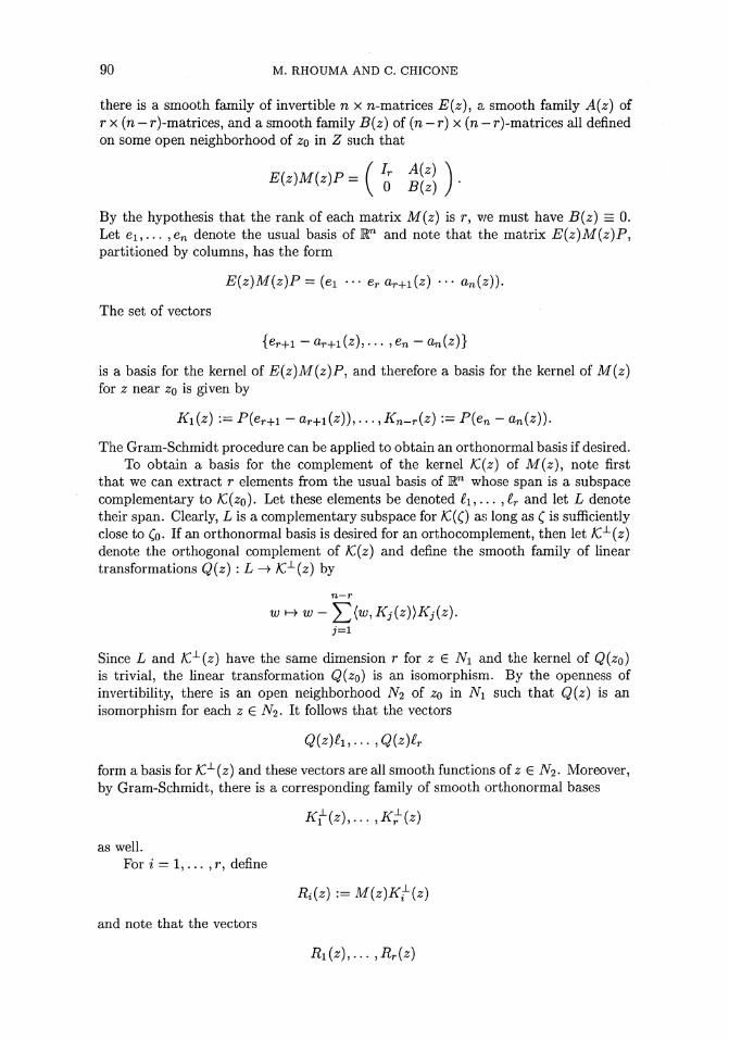
as well. For 2 = 1,... , r, define

and note that the vectors

Kt{z\...,K^{z)

Riiz) := M{z)Kt(z)


span the range of M(z). Complete this set to a basis of Mn by adding a smooth family of vectors

Rt(z),...,RJ;_r(z)

that span a complement of the range. If orthonormal vectors for an orthocomplement are desired, then use a construction similar to the construction for the orthocomplement of the kernel. In particular, there is some open neighborhood iVo of z G Z such that all of the constructed families of column vectors are smooth on iVo.

Finally, for the last statement of the proposition, let K(z) denote the matrix with columns

Kt(z),...,K^(z),K1(z),...Kn_r(z),

let R(z) denote the matrix with columns

R^z),... ,Rr(z),Ri(z),...,RJ;_r(z),

and note that if z £ No, then

M(z)K(z) = R(z)ILr.

D

3. The normally nondegenerate case. Let us assume in this section that Z is normally nondegenerate. We will determine the continuable periodic orbits in Z. Though the basic results of this section are by now well known, we will recover the standard results for the normally nondegenerate case by using a new method that will be extended to the degenerate case in the next section.

Continuations of periodic orbits corresponding to points in Z exist if and only if the displacement equation

y(NT,v,e)-v = 0

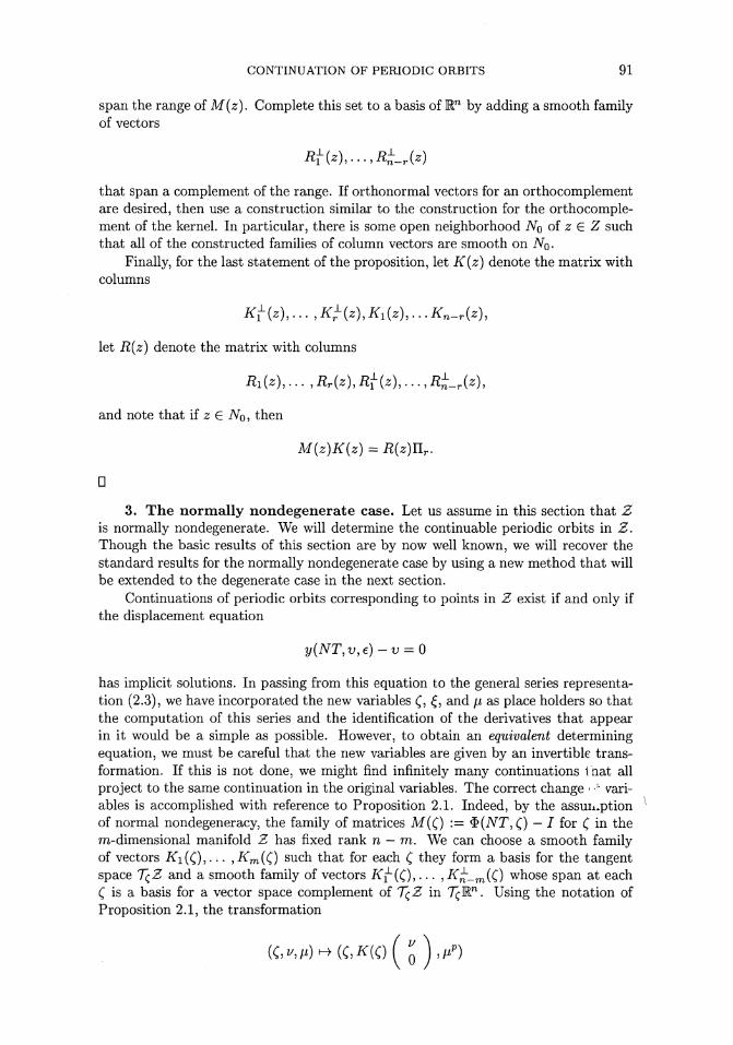
has implicit solutions. In passing from this equation to the general series representation (2.3), we have incorporated the new variables £, £, and fj, as place holders so that the computation of this series and the identification of the derivatives that appear in it would be a simple as possible. However, to obtain an equivalent determining equation, we must be careful that the new variables are given by an invertible transformation. If this is not done, we might find infinitely many continuations 1 hat all project to the same continuation in the original variables. The correct change < •*■ variables is accomplished with reference to Proposition 2.1. Indeed, by the assun.ption of normal nondegeneracy, the family of matrices M(() := $(NTX) - I for C in the m-dimensional manifold Z has fixed rank n — m. We can choose a smooth family of vectors Ki(Q,... ,i;fm(C) such that for each ( they form a basis for the tangent space T<;Z and a smooth family of vectors K^-fc),... , K^^Q whose span at each C is a basis for a vector space complement of T^Z in 7^Mn. Using the notation of Proposition 2.1, the transformation

(C,I/,/X)^(C,^(0(Q),/XP)


from Z x En~m x (0, oo) to Z x En x M is a diffeomorphism onto its image. In other words, by setting

i = K(Q ( o ) , e = Mp

with p = 1 in equation (2.4) and premultiplying by the invertible matrix family i?~1(C), this determining equation is recast in the equivalent form

0 = JR-1(C)($(iVT,C)-/)JFf(C) ( o ) +JR-1(C)2/e(^T,C,0) + O(^)

(3.i) = ( o ) +^"1(C)2/e(ivr,c,o) + 0(M).

Again, referring to the notation in Proposition 2.1, let i; E M be expressed in components t? = (t;i(C)j--- ?^n(C)) relative to the basis given by the columns of i?~1(C). Then, i?~1(C)u is precisely the vector (t>i((),... ,t>n(C))- In other words, the first n — m components of R~1(Qv is the projection of v to the range of the infinitesimal displacement <&(NT, Q — I while the last m components is the projection of v to a complement of the range. Let these two projection families be denoted by TTRCC) and 7rc(C) respectively. With this notation, the determining equation (3.1) is given by the pair of equations

0 = i/4-7rH(C)2/e(iVT,C,0) + O(/i),

(3.2) 0 = 7rc7(C)ye(^r,C,0) + O(Ai).

THEOREM 3.1. Suppose that the unperturbed system (1.1) has a normally nondegenerate, resonant period manifold Z, ^{t^Q is the principal fundamental matrix solution of the first variational equation (1.4) at ( € Z, and nciO is the corresponding projection onto the complement of the range of the infinitesimal displacement $(iVT, C) — /. If the subharmonic Melnikov function given by

(3.3) (»*c{Qvt(NT,C,0),

where

WV 1

Jo

has a simple zero (& £ Z, then Co persists.

Proof. The right hand sides of the equations in display (3.2) may be viewed as a map F of (I/,C,AO G Kn"m x Z x M to Mn-m x Mm. If Co € Z is a zero of the map (3.3), then

(3.4) i/ = I/Q := -MCotoeWfoO), z = Co, /* = 0

is a zero of F. Also, because Co is a simple zero of the second component of F, the derivative of the function given by (i/y Q ^ F(y, C, 0) when evaluated at the point (i/) C) = (I/Q, Co) can be represented as an upper triangular block matrix whose diagonal blocks are the (n — m) x (n — m) identity and the derivative of the map (3.3). Hence, by the hypothesis that Co is a simple zero of the map (3.3), the block matrix is an


invertible linear transformation from M71-771 x T^Z to En"m x Em. Therefore, by the implicit function theorem there is an implicit solution /JL H> (I/(/X),^(/X)) defined for fi in a neighborhood of /i = 0 in R such that F(i/(/i), ((//),/i) = 0 and (J>(0)>C(0))

:=

(ÔJCO)- Thus, we have proved that the point Co ^ ^ persists with the required continuation given by the curve

/iû(/x) = C(M) + ^(C(/i))('/(0/i) )

D There are other ways to state the hypothesis of Theorem 3.1 that Co is a simple

zero of the map (3.3). In particular, a useful restatement is given by the following two conditions:

(1) The vector y€(NT, Co, 0) is in the range of the matrix $(iVT, Co) - I. (2) The columns of the matrix yV€(NT,(o,Q) (the derivative of the map v H-K

ye(NT,v,0) from En to En) generate a basis of a complement of the range of the matrix $(Co, NT) - L

To prove this assertion note first that statement (1) is equivalent to the statement that Co is a zero of the map (3.3). Next, note that if T : Em -» Z is a local coordinate map given by z \-> T(z), then the corresponding local representation of the map (3.3) is given by z »-» 7Tc(T(z))ye(NT1 Y(2),0), and therefore its derivative evaluated at ZQ ^T-^Co) is given by

7rc(Co)^(ArT,Co,0)DT(zo).

Because T is a coordinate map, its derivative at ZQ has rank m. Thus, the zero is simple if and only if the composition 7rc(Co)yve{NT^Q,Q) has rank m. But, this is equivalent to statement (2).

The results of this section, albeit with different proofs, can be found along with applications to coupled oscillators in [1], [2], [3], and [4].

In the normally nondegenerate case, if condition (1) does not hold for every point Co 6 2, then none of the periodic orbits of the manifold Z persist in a smooth way; that is, there is no smooth function ft such that /3(e) = £ + e7(e) and y{NT, j3(e)y e) —(3(e) = 0. However, this leaves open the possibility that nonsmooth continuations exist; for example, continuations of the type /3(e) = C + e1^p^(e1/p) where p > 1.

Finally, we mention two possible degeneracies for our bifurcation problem. (1) The period manifold is normally degenerate. (2) Zero is a singular value of the subharmonic Melnikov function; that is, the Melnikov function has a zero Co £ Z such that the rank of the matrix 7rc(Co)yve(NT,(o^0) is less than m, or equivalently, at least one of the columns of the matrix yV€(NT, Co? O)DT(zo) is in the range of the matrix I—$(NT, Q. In the next section we will generalize Theorem 3.1 to the case of normally degenerate period manifolds. The analysis near a singularity of the Melnikov function is beyond the scope of this paper.

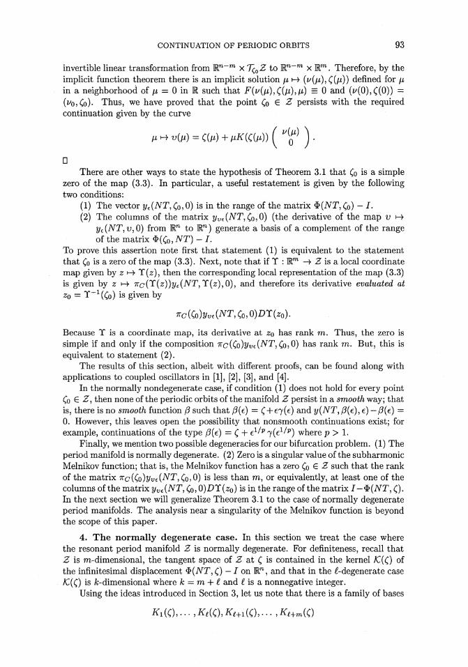
4. The normally degenerate case. In this section we treat the case where the resonant period manifold Z is normally degenerate. For definiteness, recall that Z is m-dimensional, the tangent space of Z at C is contained in the kernel /C(C) of the infinitesimal displacement <I>(7VT, C) — / on En, and that in the ^-degenerate case /C(C) is ^-dimensional where k — m -f £ and £ is a nonnegative integer.

Using the ideas introduced in Section 3, let us note that there is a family of bases

Ifl(C),..., ^(0,^+1(0, • ••,tf*+m(0


for the kernel of the infinitesimal displacement as in Proposition 2.1 such that the last m vectors form a basis for the tangent space of Z at £• For a notational convenience, let V : M72-* x E£ -+ W1^ x R1 x lRm denote the inclusion given by

(z/, K) »->• (l/, AC,0).

The transformation

viewed as a map from Z x E71-* x E^ x (0, oo) to Z x En x E, or alternatively, as a map from iT x Wl~k x E^ x (—oo,0) to Z x En x E, is a diffeomorphism onto its image. In other words, if we consider either /x > 0 or // < 0, set

(i = K{QV{v,K), e = v?

with p = 2 in the determining equation (2.5), and premultiply by the invertible matrix family JR~

1(C), then equation (2.5) is recast into the equivalent form

+ lyvv(NT,<:,0)(m)V(u,K))2)+O(^)

u\ . ( KR{Q{yt + \yvv{KVY) (41) -V')+>W^&™r>r'w

where the arguments of some of the functions in the order // terms of the second equation have been suppressed, and the projections KR^) and 7rc(C) as in Section 3 are the projections onto the range and the complement of the range of the infinitesimal displacement corresponding to the matrix R~l(C).

Let us define the generalized subharmonic Melnikov function M : Z x E^ —> Rk

by

(4.2) M(C,K) = irc(O{ye(NT,<;,0) + ^w(iVT,C,0)(^(C)F(0,K))2).

The integral expressions for the partial derivatives that appear in this expression are given by formulas (2.7) and (2.8). We note that in the formula for M only the first term depends on the perturbation. Also, we note that

£

(4.3) K(QV(0,K) = Y,KiKi(Q i=l

where K = (ACI, ... , KI) and iî(C)> • • • > ^(0 is a basis for a vector space complement of the tangent space of Z at £ in the kernel )C(Q of the infinitesimal displacement. Finally we mention that if I = 0, then Z is normally nondegenerate and the function M reduces to the corresponding function (3.3).

THEOREM 4.1. If Z is an ^-degenerate resonant period manifold for the unperturbed system (1.1) and if (Ccbô) € Z x E^ is a simple zero of the generalized subharmonic Melnikov function M defined in display (4-2), then (o persists. More- over, there are two continuation curves both defined for e > 0.


Proof. Note that for ji ^ 0 the solutions of the determining equation (4.1) correspond to the zeros of the function F : JT-* x Z x M* x E -+ W1-* x Rk obtained by dividing the second component of the right hand side of equation (4.1) by ^. If fact, F is of the form

F(I/,C,/6,M) = (^MC,«)) + 0(M).

If .M(Cojfto) = 0* then F(0,Co,^0,0) = 0. Also, because (COJÔ) is a simple zero of M, the derivative of the function (i/,C>^) ^ -^(^JCJ^JO) evaluated at the point (0, Co, fto) is the invertible linear transformation from W1'1" xT^ZxW- to W1'1" x M* represented in matrix form by

In-k 0 0 0 A1c(Co,ô) A^/cCCoô)

Thus, by the implicit function theorem, there is an implicit solution y, H-> (^(/x),C(^),^(/i)) defined in some neighborhood of /x = 0 such that F(V(IJ,),((/J,), K(fj,),y) = 0 and (z/(0),C(0), AC(0)) = (0,Co,ô)- The two required continuations are given by

u = cOi) + /itf(CMWi/(MM/i))

with /x = i^/e and e G [0, e*) for some e* > 0. D

REMARK 4.2. Let us recall that in our original system (1.1), the parameter e is assumed to be nonnegative. However, we can easily consider nonpositive e by applying our results to the system

y = f(y)+£9(t,y,e)

where e = -e and g(t,y,e) = —g(t,y, —e). The important point is that

j/ff(JVr,i;,0) = -y€(JVT,t;,0).

Thus, the generalized Melnikov function is replaced by the function M- : ZxB? —> Rk

where

M-(C,K) := 7rc(C)( - V<(NT,C,0) + \yvv(NT,C,0)^(0^(0,K))2).

A simple zero of either M or M- corresponds to a continuation of a periodic orbit for system (1.2). The domain of the continuation corresponding to M has e > 0 while the domain of the continuation corresponding to M- has e < 0. As we will illustrate in Section 7, it is very likely that the simple zeros of M and M- are different.

REMARK 4.3. To apply our results, the fundamental matrix $(NT,Q of the first variational equation along the unperturbed resonant periodic solutions must be "known". Of course, for most nonlinear systems this requirement is impossible to meet. However, we note that the variational equations for a planar system can be reduced to quadratures along the unperturbed period solutions. In fact, Diliberto's theorem [10] provides formulas for the integration of the homogeneous variational equations of a plane autonomous differential equation in terms of geometric quantities defined along the unperturbed orbit (see the results in [1, 2, 3, 4]). This fact can be


very useful in the analysis of planar systems and weakly coupled planar systems. Unfortunately, we do not know how to obtain a substitute for Diliberto's theorem in En for n > 2.

REMARK 4.4. In our analysis we use the assumption that the dimension of the kernel IC(Q of the infinitesimal displacement $(iVT, () — I is constant for £ in ?.n open neighborhood in the resonant period manifold. Without this assumption, we cannot prove the existence of the smooth families of matrices R(Q and K(£). It is easy to construct a period manifold where the dimension of the kernel of the infinitesimal displacement is not constant. For example, consider the system

x = y — xz(x2 +y2 — 1),

y = -x-yz(x2 + y2 -1),

(4.4) z = 0,

and note that the set {(#, y, z) : x2+y2 — 1} is a two-dimensional, 27r-period manifold. Whereas the kernel of the infinitesimal displacement is two-dimensional at each point of the subset 5i := {(#, y, z) : x2 + y2 = 1, z > 0}, the kernel is three-dimensional on the subset 52 := {(x,y,z) : x2 -f- y2 = 1, z = 0}. Of course, Si is itself a normally nondegenerate, two-dimensional period manifold while 52 is a two-degenerate, one- dimensional period manifold. Our general results can be used to analyze continuations of periodic orbits for perturbations of system (4.4) by considering three different period manifolds corresponding to the periodic orbits with z > 0, z = 0, and z < 0.

5. Cronin's Theorem. We will point out an oversight in [7] where the continuation of periodic solutions is studied for n-dimensional first order systems of the form

(5-1) § = /(*)+S(*,A0

with the following assumptions: (1) The function t H* g(t,/i) is periodic with period T(^) where T(/J,)—T = 0(/i3)

and T = T(0) is the period of a periodic orbit F of the unperturbed system

if* = o)- (2) There is a smooth function g(t,ix) such that #(£,//) = Li2g(t,ii). (3) For £ G F, the eigenvalue one of the principal fundamental matrix $(T, £)

has algebraic multiplicity one. By the first and second assumptions, equation (5.1) can be written in the form

(5.2) § = /(*)+Ai2s(t,A0

where t i-» g(t,/j,) is periodic with period T(/i). Assumption (3) states that the kernel of the matrix I — $(T, Q is one-dimensional. In other words, F is a normally nondegenerate, resonant period manifold.

The result of the continuation analysis in [7] is a bifurcation equation of the form

(5.3) Ay2 + B = 0

where (translating to our notation) y G E,

A = 7rc(0 / $(T,O*-Hs,OD2f(x(s,<;,0){$(s,Of(O)2ds, Jo


and

Jo

In [7] the quantities A and B are not viewed as functions of f. On page 378 in [7] the author claims that a simple zero of (5.3) (viewed as an equation for the variable 2/), corresponds to a continuable periodic orbit of the unperturbed system. By adding a fourth assumption, namely —B/A > 0, it is observed that the bifurcation equation (5.3) does in fact have simple zeros. However, by Proposition 5.1 below, A — 0. Thus, the continuation theorem in [7] is logically correct, but vacuous. In fact, equation (5.3) always reduces to the equation B = 0. If this equation is viewed as an equation for £ G F, then the result in [7] can be reinterpreted to be in complete agreement with Theorem 3.1. In effect, if the function ( «-> B(Q has a simple zero ZQ £ F, then there is a one-parameter family with parameter JJ, of perturbed periodic orbits in the extended phase space and a corresponding family of initial conditions v(fij such that v(Q) = Co- In this sense, if B has a simple zero, then F persists.

The fact that A = 0 is a special case of a more general result that we will now formulate and prove.

Using the notation of Section 4, let us assume that Z is an m-dimensional, resonant period manifold for the n-dimensional, first order system y = f(y) with the solution family 11-* y(t,v) defined so that 2/(0,v) = v. By Proposition 2.1, there is a smooth family of bases

for the kernel JC(Q of the infinitesimal displacement / — $(NT, () such that the last m vectors are tangent to Z. If u € /C(0, then u = nnor(C) + utan(C) where unor(0 is in the span of the first £ basis vectors and u = ân(C) is in the span of the last m basis vectors.

PROPOSITION 5.1. //( e Z, then

7rc(0^(^,0(^tan(0^tan(0) - 0

and

Kc(Oyvv(NT,<;)(utaa(0,unov(0) = o.

Proof. Because tran(0 is in 7^ Z, there is a smooth curve s ^ f (s) in En whose range is in Z such that £(0) = C and £(0) = iran(0. Moreover, for each s in the domain of this curve, the function t \-> y(t, £(s)) is a periodic solution of system (1.2). In particular, we have that

(5.4) y(NT,Z(8))-ti8) = 0.

By computing the second derivative with respect to the variable s, we obtain the identity

(5.5) yvv(NT, ^(s)) (Us), fa)) + yv(NT, 0, £(*))!(«) - fa) = 0.


Also, let us recall that

yv(NT,m) = mT,0-

Thus, equation (5.5) can be rewritten as

(5.6) {I-$(NT,0)Z"(s) = Vw(NT,tt8)){foU(s)),

and we obtain the identity

;r HOWivr, o («tan(C)^tan(0)

Recall that for v G W1 the vector 7rc(0v '1S Just ê vector in Rk given by the last k components of R~1(Qv. Since the last k components of the vector nn_&if "^((^"(O) all vanish, we have proved the first equality of the proposition.

To prove the second equality of the proposition, define the smooth curve s *-»■ 7(5) in Mn by

7W:=^n0rttW)

and note that 7(0) = unOT((). Also, note that the vector 7(5) is in the kernel /C(£(s)) of J — $(iVT, £(s)) for all s in the domain of the curve £. Hence, we have that

(yv(NT,t(s))-Ih(s) = 0.

Differentiate both sides of this identity with respect to 5 and evaluate at s = 0 to obtain the equation

yvv(NT,0(ut&n(0,unor(0) + {yv(NT,0 - 1)7(0) = 0.

The proof of the second equality of the proposition is completed exactly as the proof of the first equality is completed from equation (5.6). □

To prove that A — 0 for the system dx/dt = /(#), note that the vector $(5, C)/(C) = f(x(s, C)0)) is everywhere tangent to the period manifold T and then use Proposi- tion 5.1.

6. Discussion. In this section we will briefly discuss the consequences of the substitution e = fip in equation (2.2) where p > 1 is a rational number. Also, we will describe the main result of the continuation theory in case the unperturbed system is linear.

The restriction p > 1 is important for our analysis of the case where the infinitesimal displacement is not the zero map for at least two reasons: We must be able to divide equation (2.2) by /i without introducing a singularity in equation (2.3). The leading term in equation (2.3) must be yv(NT, (, 0) - I so that the same steps as in the proof of Theorem 4.1 can be followed. Also, it is convenient to consider four cases: p = 1, 1 < p < 2, p = 2, and p > 2.

If p = a/6, the integers a and b have no common factors, and 1 < p < 2, then equation (2.3) can be studied in the form

0 = (yv(NT, C, 0) - I)£ + â-^bye(NT, C, 0) + 0{fi).


For b ^ 1, the right hand side of this equation may not be smooth. But, this problem can be overcome by considering a new small parameter p = /j}^b and the substitution £ = K(QV(v, K) where K and V are the functions defined in Section 4. Furthermore, just as in Section 4, it suffices to find an implicit solution of the determining equations

v\ . a-bf **(C)!/«(MZ\C,0) \

Here, under the assumption that £ H* 7rc(C))2/€(-WT, C,0) has a zero £o> we can solve implicitly for i/ in the first component equation. The second equation (after substitution of the implicit solution and division by /xa~6) has values in E^ where k is the dimension of the kernel of the infinitesimal displacement. But £ G Z is locally in Em

with k = m + L Thus, the implicit function theorem does not apply unless C = 0 in which case we revert to the subharmonic Melnikov function obtained for p = 1. In fact, we must obtain the same continuations already determined for this case.

If p > 2, then equation (2.3) can be studied in the form

0 = (yv(NT, C, 0) - /)£ + \wvv(NTt C, 0)£2 + O(iS).

Again, with p, z/, and K as for the case 1 < p < 2, we have the determining equation

This case appears to lead to a "generalized Melnikov function" that is simpler than the one obtained in Section 4. Indeed, a simple zero (Co, ô) of the function

(C,«) H> 7rc(C)(^(ivr,c,o)(i^cmo,*))2) persists. However, because this function is homogeneous in K, if (Co,ô) is a zero, then so is (Co,^ô) for a E M. Thus, this function cannot have a simple zero.

If the unperturbed system is linear, then the second order derivative yvv(NT, £, 0) and all higher order derivatives of y with respect to the space variable v evaluated at v = £ vanish. Because of this fact, the continuation problem can often be simplified. Consider the classic model of the periodically forced planar oscillator

(6.1) y = Ay + eg(t,yre)

where A is a matrix of constants (see, for example, [5, 6, 8, 16, 18, 19, 20]). For the most important special case

and the infinitesimal displacement I — $(27r,C) is identically zero. By setting p = 1 and dividing by a power of /i in equation (2.3), we find immediately that it suffices to solve the determining equation

0 = 2/€(iVT,C,0) + O(e).

In this case ( E M2, so no projection is necessary. Thus, we recover the following classic result: // the function C >-> -2/e(iVT, £,0) has a simple zero, then the corresponding unperturbed periodic solution persists.


REMARK 6.1. The concept of a "controllably" periodic perturbation has been introduced and studied in [12, 13, 14]. The period of the perturbation is allowed to vary. In these systems, the perturbation function #, in our notation, can be written as

9(t,y,e)=g(t/T,y,€,T)

where

g(8 + l,y,e9T) = g(s,y,e,T).

The continuation theory for periodic orbits of such systems is developed under the assumption that the number one is a simple eigenvalue of $(T, £). Our analysis can be used to extend this result to include the case where one is not a simple eigenvalue.

7. Examples. We will use the first order system

x = y — x(x2 + y2 - I)2 — e cos £,

y = -x - y(x2 + y2 - l)2+esin£,

(7.1) z = z(x2 +y2) + 6smt

(a modification of a differential equation studied in [3]) to illustrate the continuation of periodic orbits for the normally degenerate case.

The unperturbed system (7.1) has the resonant period manifold

Z := {(x, y, z) : x2 + y2 = 1, z = 0},

consisting of a single periodic orbit. Let us consider the following family of unperturbed solutions on Z:

t \-> (cos(t -6),- sm(t - (9), 0)

where 9 is the usual angular variable. To be completely compatible with the notation used in the general theory, we would have to write this family as

t ^ (cos(t - C), - sin(£ -0,0)

where C = (cos 8, sin #,0). Our first choice amounts to a choice of a local (angular) coordinate on Z.

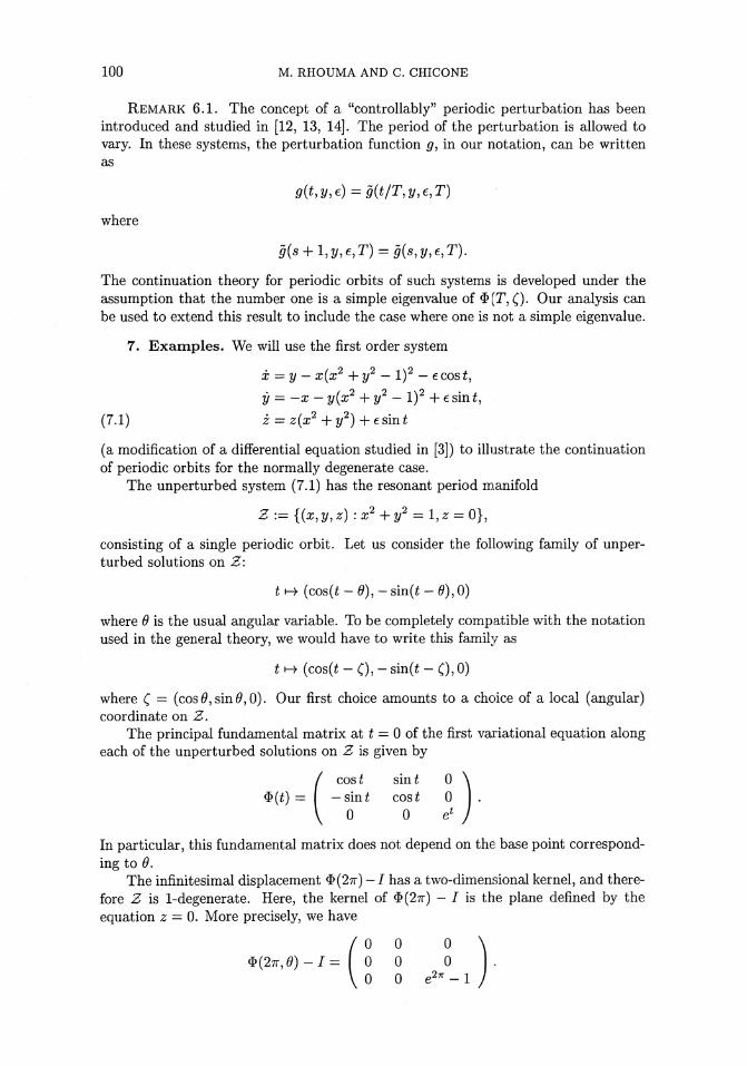
The principal fundamental matrix at t = 0 of the first variational equation along each of the unperturbed solutions on Z is given by

0 0

In particular, this fundamental matrix does not depend on the base point corresponding to 6.

The infinitesimal displacement $(27r) - / has a two-dimensional kernel, and therefore Z is 1-degenerate. Here, the kernel of $(27r) - / is the plane defined by the equation z = 0. More precisely, we have

/ 0 0 0 *(27r,0)-J= 0 0 0

\ 0 0 e277 - :


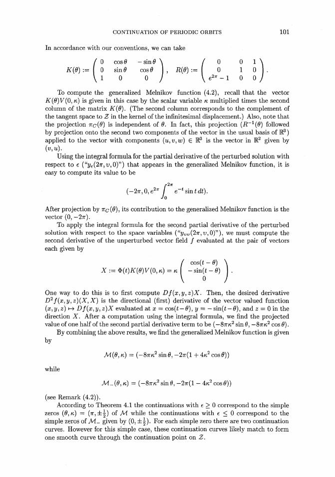
In accordance with our conventions, we can take

0 COS0 -sin( 0 sin0 COS0

1 0 0

0 0 1 0 1 0

,2n_1 0 0 K(0):= 0 sin/9 cos9 , R(9) :=

To compute the generalized Melnikov function (4.2), recall that the vector K(0)V(0, K) is given in this case by the scalar variable hi multiplied times the second column of the matrix K(6). (The second column corresponds to the complement of the tangent space to Z in the kernel of the infinitesimal displacement.) Also, note that the projection nc{0) is independent of 6. In fact, this projection (R~1(0) followed by projection onto the second two components of the vector in the usual basis of E3) applied to the vector with components (u,v,w) 6 M3 is the vector in M2 given by (V,u).

Using the integral formula for the partial derivative of the perturbed solution with respect to e ("t/e(27r,'U,0)") that appears in the generalized Melnikov function, it is easy to compute its value to be

(-27r,0,e27r / 27r

-t e sintdt).

After projection by 7rc(#), its contribution to the generalized Melnikov function is the vector (0, — 27r).

To apply the integral formula for the second partial derivative of the perturbed solution with respect to the space variables ("yvv(27r,v,0)n), we must compute the second derivative of the unperturbed vector field / evaluated at the pair of vectors each given by

/ cos(*-0) X:=Q(t)K(0)V(Q,K)=K\ -sin(t-0)

V o One way to do this is to first compute Df(x1y,z)X. Then, the desired derivative D2f(x,y,z)(XyX) is the directional (first) derivative of the vector valued function (x,y.,z) i-> Df(xJy,z)X evaluated at x = cos(t — 0), y = -sm(t — 9), and z = 0 in the direction X. After a computation using the integral formula, we find the projected value of one half of the second partial derivative term to be (—STTK

2 sin 0, —STTK

2 COS 0).

By combining the above results, we find the generalized Melnikov function is given by

M(0, K) = (STTK2 sin0, -2ir(l + 4AV

2 COS0))

while

M-(0,K) = (STTK2 sin(9, -27r(l - 4K;

2 COS0))

(see Remark (4.2)). According to Theorem 4.1 the continuations with e > 0 correspond to the simple

zeros (0, rc) = (TT, ±|) of M while the continuations with e < 0 correspond to the simple zeros of M- given by (0, ±|). For each simple zero there are two continuation curves. However for this simple case, these continuation curves likely match to form one smooth curve through the continuation point on Z.


Our second example is a system of m coupled oscillators; the jth oscillator has the form

ij = VjUj -XJ(

XJ +yj -^j) + mj(t,xi, > - - ,xm,yi, > - - ,ym,e),

Vj = -VjXj - Vjitf + v) - tf)2 + e92,j(t,a:i,...,xm,yu...,ym,e)

where /x^ and Xj are nonzero constants. Let us assume that the unperturbed oscillators are all in resonance, and therefore they have a smallest common period TQ. Then, the unperturbed system has an m-dimensional torus Z as a period manifold; Z is the product of limit cycles, one for each of the m uncoupled planar oscillators. Let us also consider the family of unperturbed solutions on Z

given by

t h+ (xi (*), 2/1 (*),..., xm(t),ym(t))

Xjit) = Xj cosfajt - Oj), yj(t) = -Xj sinfajt - 6j)

where 6j is an angular variable and 0 := (#i,... ,#m) is the local angular coordinate on Z.

The period manifold Z is m-degenerate. In fact, the kernel of infinitesimal displacement $(To, 0) - / is all of M2m. The projection 7rc(C) onto the complement of the range of the infinitesimal displacement is the identity map. Notice that in this case t = m. Hence, the function V maps Mm to Mm x Em and we have that

$(t,&)K(Q)V(K) =

—Ki sin(/ii^ — #i)

K>m COS(/Xm6 — Um)

\-Km Sm(fJLmt - dm)J

where K = (ACI, ... ,/cm). If we also assume that each function ^?J- is time-periodic with a smallest common period T such that MTQ = NT for some relatively prime integers M and iV, then after a straightforward computation we find that

(7.2)

where

(7.3)

and

M±(Q,K) = -4NT

Pifl Jo Vs1 COSjljS

sm/j,jS

( Af^cosî ^ Af/cf sin0i

Af/c^cos0n

VAf^sini9m/

— smfijS

COSfijS

Pi,2

Pm,l \PrnaJ

gj,2{s,XQ{s),Y0{s),0)

XQ{S) = (Ai cosQuis -i9i),...,Amcos(^m5 -<9m)),

YQ(S) = ( - Ai sindiis - 0i),..., -Am sm(fjLms - 0m)).


Thus, if the system of m equations, consisting of the pairs of equations

-4NT\$K% cos Oj ± pj,! = 0, -ANTX^^j sin Oj ± pja = 0

with one fixed choice of sign for j = 1,... , m, has a simple zero (0o, fto) ^ % x ^m, then the corresponding unperturbed periodic orbit through ©o persists.

At a continuation point there can be as many as 2m corresponding continuation curves. For example, if we set m = 2 and fij = Xj — 1 for j — 1,2, and if we let

#l,l(î,?/i,£2,2/2,e) =0, 01,2(*,Sl,2/l,a2,J/2,e) =»2)

P2,i(*>a?i>2/i>^2,2/2,c) = 0, #2,2(^^1,2/1, ^2,2/2, c) = -si +acos£,

then the generalized Melnikov function for e > 0 is given by

(7.4) M(0,«) =

/ — 87rttf cos 61 —TT sin ^2 \ -STTÎ sin ^1 + TT cos 62 —STT^ cos ^2 + TT sin #1

\—STT^ sin 62 — TT cos ^1 + Tray

When 0 < |a| < 1, the function M(Q,K) does in fact have eight simple zeros corresponding to two continuation points on the original unperturbed torus, namely,

(O,K) = (0,-l±iV2,±lvr^)

and

(e)K)=(7r>|)±^>/2,±ivT+^).

Also, when 0 < |a| < 1, the function M-(Q,K) for e < 0 has eight different simple zeros, namely,

(e,K)=(Q,?ri±]y/2,±\y/T^)

and

Notice that at each continuation point ©o on the unperturbed torus, there are 2m = 4 possible directions £ G M4 along which a continuation curve exists. For instance, at the point (^1,^2) = (0, — 7r/2) continuation curves exist along the directions

ACKNOWLEDGMENTS. We thank the referees for several helpful suggestions.

REFERENCES

[1] C. CHICONE, Lyapanov-Schmidt reduction and Melnikov integrals for bifurcation of periodic solutions in coupled oscillators, J. Diff. Eqns., 112:2 (1994), pp. 407-447.

[2] C. CHICONE, A geometric approach to regular perturbation theory with an application to hy- drodynamics, Trans. Amer. Math. Soc, 347:12 (1995), pp. 4559-4598.


[3] C. CHICONE, Bifurcations of nonlinear oscillations and frequency entrainment near resonance, SIAM J. Math. Anal, 23 (1992), pp. 1577-1608.

[4] C. CHICONE, Periodic solutions of a system of coupled oscillators near resonance, SIAM J. Math. Anal, 6 (1995), pp. 1257-1283.

[5] C. CHICONE, Ordinary Differential Equations With Applications, Texts in Applied Math., Springer-Verlag, New York, 1999.

[6] E. A. CODDINGTON AND N. LEVINSON, Theory of Ordinary Differential Equations, McGraw- Hill, New York, 1955.

[7] J. CRONIN, Entrainment of frequency in singularly perturbed systems, Methods and Applica- tions of Analysis, 3 (1996), pp. 370-400.

[8] J. CRONIN, Quasilinear equations and equations with large nonlinearities, Rocky Mountain J. Math, 4 (1974), pp. 41-63.

[9] A. DEVINATZ, Advanced Calculus, Holt, Rinehart and Winston, Inc, 1968. [10] S. P. DILIBERTO, On systems of ordinary differential equations, in Contributions to the Theory

of Nonlinear Oscillations, Annals of Mathematics Studies 20, Princeton University Press, Princeton, NJ, 1950.

[11] G. B. ERMENTROUT, n:m Phase-locking of weakly coupled Oscillators, J. Math. Biology, 12 (1981), pp. 327-342.

[12] M. FARKAS, Controllably periodic perturbations of autonomous systems, Acta Math. Acad. Sci Hung, 22 (1971), pp. 337-348.

[13] M. FARKAS, Determination of controllably periodic perturbed solutions by Poincare's method, Studia Sci Math. Hung, 7 (1972), pp. 257-266.

[14] M. FARKAS, On isolated periodic solutions of differential systems, Ann Mat. Pura. Appl, 106 (1975), pp. 233-243.

[15] M. FARKAS, Estimates on the existence regions of perturbed periodic solutions, SIAM J. Math. Anal, 9:5 (1978), pp. 876-890.

[16] M. FARKAS, Periodic Motions, Springer-Verlag, 1994. [17] J. K. HALE AND P. Z. TABOAS, Interaction of damping and forcing in a second order equation,

Nonlin. Anal: Theory, Meth. Appl., 2 (1978), pp. 77-84. [18] A. NAYFEH AND D. MOOK, Nonlinear Oscillations, John Wiley, New York, 1979. [19] M. ROUSEAU, Vibrations in Mechanical Systems, Springer-Verlag, 1987. [20] J. MAWHIN AND N. ROUCHE, Equations differentielles ordinaires, Masson, Paris, 1973. [21] M. M. VAINBERG AND V. A. TRENOGIN, Theory of Branching of Solutions of Non-linear Equa-

tions, Noordhoff International Publishing, 1974.

Documents

ON THE CONTINUATION OF PERIODIC ORBITS* 1. Introduction