ON THE CONSTITUTIVE MODELING AND NUMERICAL … · Kuhn-Tucker conditions: ff≤≥ =0, 0, 0ζζ&& Norm operator: ‖QQQD‖= DD: We now treat the nonlinear problem summarized in Table

S(3)T2010 - Smart Structural Systems Technologies 1

ON THE CONSTITUTIVE MODELING AND NUMERICAL IMPLEMENTATION OF SHAPE MEMORY ALLOYS UNDER

MULTIAXIAL LOADINGS - PART II: NUMERICAL IMPLEMENTATION AND SIMULATIONS

J. ARGHAVANI PhD student Sharif University of Technology Tehran – Iran

F. AURICCHIO Professor University of PaviaPavia – Italy

R. NAGHDABADI Professor Sharif University of Technology Tehran – Iran

A. REALI Assistant Professor University of Pavia Pavia – Italy

ABSTRACT In Part I, we developed several constitutive models at small and finite strain regimes. In this part, we present the numerical counterpart and investigate solution algorithm, its robustness as well as computational cost or efficiency for a finite strain constitutive model, knowing that similar discussion is used for a small strain model. For this purpose, we specifically focus on the finite strain extension of the model proposed by Souza et al, developed in Part I. We start proposing a time integration scheme and developing time-discrete constitutive model. We then construct the solution algorithm and study the robustness of different algorithms through several benchmark tests at gauss point level. In order to study the algorithms efficiency, we implement the developed solution algorithm into a user defined subroutine UMAT in the nonlinear finite element program ABAQUS and simulate several boundary value problems. We then evaluate the algorithms efficiency comparing solution CPU times of different algorithms. The simulation results show that the developed finite strain constitutive model and its corresponding solution algorithm provide an appropriate computational tool which can be used to design, analysis and optimize SMA-based devices.

2 S(3)T2010 - Smart Structural Systems Technologies

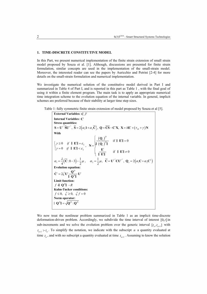
1. TIME-DISCRETE CONSTITUTIVE MODEL In this Part, we present numerical implementation of the finite strain extension of small strain model proposed by Souza et al. [1]. Although, discussions are presented for finite strain formulation, similar concepts are used in the implementation of the small-strain model. Moreover, the interested reader can see the papers by Auricchio and Petrini [2-4] for more details on the small-strain formulation and numerical implementation. We investigate the numerical solution of the constitutive model derived in Part I and summarized in Table 4 of Part I, and is reported in this part as Table 1 , with the final goal of using it within a finite element program. The main task is to apply an appropriate numerical time integration scheme to the evolution equation of the internal variable. In general, implicit schemes are preferred because of their stability at larger time step sizes.

Table 1: fully symmetric finite strain extension of model proposed by Souza et al [5]. External Variables: ,TC

Internal Variables: tC Stress quantities:

( ) ( )1 1

1 22, , ,t t t tMhα α τ γ

− −

= = + = − = + +S U SU S 1 C Q CS C X X E N

With

( )( )

if 00

,0

if 0

De t

DtL e

t tL tt

ifif

γ εγ ε

⎧=⎪

⎧ ≥ = ⎪=⎨ ⎨= <⎩ ⎪

≠⎪⎩

QE

E QNE E E

E

‖ ‖‖ ‖ ‖ ‖‖ ‖

‖ ‖‖ ‖

( ) ( )1 1 21 2 1 2

1 1: 3 , , 24 2 2

,t te

λα μ α μ α α− −

= − − = = = +C 1 C U CU Q C C

Evolution equation:

2D

t t tDζ=C QU U

Q& &

‖ ‖

Limit function: Df R= −Q‖ ‖

Kuhn-Tucker conditions: 0, 0, 0f fζ ζ≤ ≥ =& &

Norm operator:

:D D D=Q Q Q‖ ‖

We now treat the nonlinear problem summarized in Table 1 as an implicit time-discrete deformation-driven problem. Accordingly, we subdivide the time interval of interest [0, ]t in sub-increments and we solve the evolution problem over the generic interval 1[ , ]n nt t + with

1n nt t+ > . To simplify the notation, we indicate with the subscript n a quantity evaluated at time nt , and with no subscript a quantity evaluated at time 1nt + . Assuming to know the solution


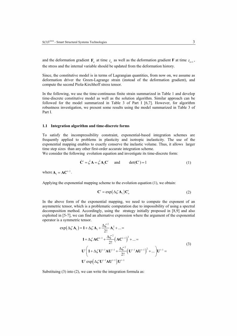
and the deformation gradient nF at time nt as well as the deformation gradient F at time 1nt + , the stress and the internal variable should be updated from the deformation history. Since, the constitutive model is in terms of Lagrangian quantities, from now on, we assume as deformation driver the Green-Lagrange strain (instead of the deformation gradient), and compute the second Piola-Kirchhoff stress tensor. In the following, we use the time-continuous finite strain summarized in Table 1 and develop time-discrete constitutive model as well as the solution algorithm. Similar approach can be followed for the model summarized in Table 3 of Part I [6,7]. However, for algorithm robustness investigation, we present some results using the model summarized in Table 3 of Part I. 1.1 Integration algorithm and time-discrete forms To satisfy the incompressibility constraint, exponential-based integration schemes are frequently applied to problems in plasticity and isotropic inelasticity. The use of the exponential mapping enables to exactly conserve the inelastic volume. Thus, it allows larger time step sizes than any other first-order accurate integration scheme. We consider the following evolution equation and investigate its time-discrete form:

1 and det( ) 1t t tζ ζ= = =C A A C C& & & (1) where 1

1t−=A AC .

Applying the exponential mapping scheme to the evolution equation (1), we obtain:

( )1expt tnζ= ΔC A C (2)

In the above form of the exponential mapping, we need to compute the exponent of an asymmetric tensor, which is a problematic computation due to impossibility of using a spectral decomposition method. Accordingly, using the strategy initially proposed in [8,9] and also exploited in [5-7], we can find an alternative expression where the argument of the exponential operator is a symmetric tensor.

( )

( )

( )

( )

22

1 1 1

2 21 1

2 21 1 1 1 1

1 1 1

exp ...2!

...2!

...2!

exp

t t

t t t t t t

t t t t

ζζ ζ

ζζ

ζζ

ζ

− −

− − − − −

− − −

ΔΔ = + Δ + + =

Δ+ Δ + + =

⎛ ⎞Δ+ Δ + + =⎜ ⎟

⎝ ⎠

Δ

A 1 A A

1 AC AC

U 1 U AU U AU U

U U AU U

(3)

Substituing (3) into (2), we can write the integration formula as:


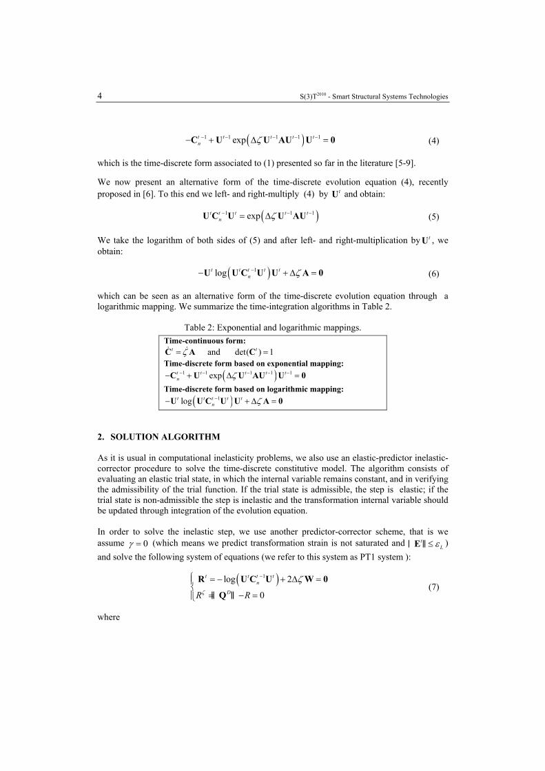
( )1 1 1 1 1expt t t t tn ζ− − − − −− + Δ =C U U AU U 0 (4)

which is the time-discrete form associated to (1) presented so far in the literature [5-9]. We now present an alternative form of the time-discrete evolution equation (4), recently proposed in [6]. To this end we left- and right-multiply (4) by tU and obtain:

( )1 1 1expt t t t tn ζ− − −= ΔU C U U AU (5)

We take the logarithm of both sides of (5) and after left- and right-multiplication by tU , we obtain:

( )1logt t t t tn ζ−− + Δ =U U C U U A 0 (6)

which can be seen as an alternative form of the time-discrete evolution equation through a logarithmic mapping. We summarize the time-integration algorithms in Table 2.

Table 2: Exponential and logarithmic mappings. Time-continuous form:

and det( ) 1t tζ= =C A C& & Time-discrete form based on exponential mapping:

( )1 1 1 1 1expt t t t tn ζ− − − − −− + Δ =C U U AU U 0

Time-discrete form based on logarithmic mapping: ( )1logt t t t t

n ζ−− + Δ =U U C U U A 0

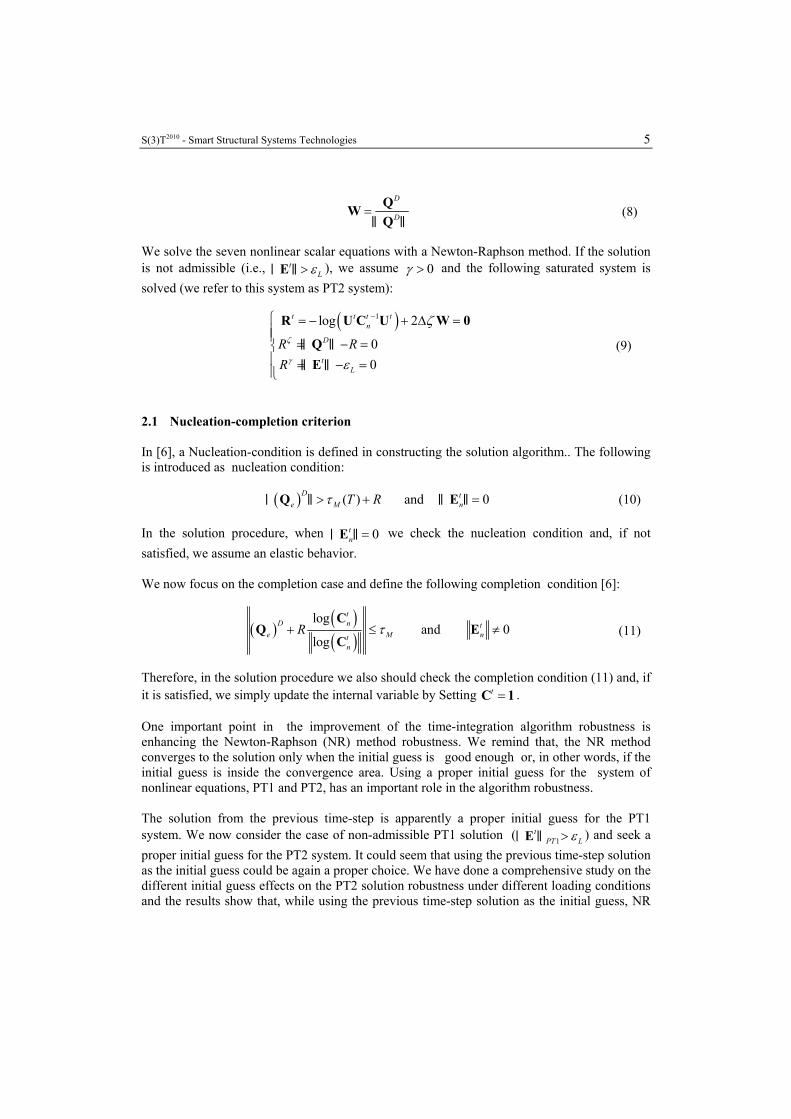
2. SOLUTION ALGORITHM As it is usual in computational inelasticity problems, we also use an elastic-predictor inelastic-corrector procedure to solve the time-discrete constitutive model. The algorithm consists of evaluating an elastic trial state, in which the internal variable remains constant, and in verifying the admissibility of the trial function. If the trial state is admissible, the step is elastic; if the trial state is non-admissible the step is inelastic and the transformation internal variable should be updated through integration of the evolution equation. In order to solve the inelastic step, we use another predictor-corrector scheme, that is we assume 0γ = (which means we predict transformation strain is not saturated and t

Lε≤E‖ ‖ ) and solve the following system of equations (we refer to this system as PT1 system ):

( )1log 2

0

t t t tn

DR Rζ

ζ−⎧ = − + Δ =⎪⎨

= − =⎪⎩

R U C U W 0

Q‖ ‖ (7)

where


D

D=QWQ‖ ‖

(8)

We solve the seven nonlinear scalar equations with a Newton-Raphson method. If the solution is not admissible (i.e., t

Lε>E‖ ‖ ), we assume 0γ > and the following saturated system is solved (we refer to this system as PT2 system):

( )1log 2

00

t t t tn

D

tL

R RR

ζ

γ

ζ

ε

−= − + Δ =⎧

= − == − =

⎪⎪⎨⎪⎪⎩

R U C U W 0

QE

‖ ‖‖ ‖

(9)

2.1 Nucleation-completion criterion In [6], a Nucleation-condition is defined in constructing the solution algorithm.. The following is introduced as nucleation condition:

( ) ( ) and 0 D te M nT Rτ> + =Q E‖ ‖ ‖ ‖ (10)

In the solution procedure, when 0t

n =E‖ ‖ we check the nucleation condition and, if not satisfied, we assume an elastic behavior. We now focus on the completion case and define the following completion condition [6]:

( ) ( )( )

logand 0

log

tD n t

e M ntn

R τ+ ≤ ≠C

Q EC

(11)

Therefore, in the solution procedure we also should check the completion condition (11) and, if it is satisfied, we simply update the internal variable by Setting t =C 1 . One important point in the improvement of the time-integration algorithm robustness is enhancing the Newton-Raphson (NR) method robustness. We remind that, the NR method converges to the solution only when the initial guess is good enough or, in other words, if the initial guess is inside the convergence area. Using a proper initial guess for the system of nonlinear equations, PT1 and PT2, has an important role in the algorithm robustness. The solution from the previous time-step is apparently a proper initial guess for the PT1 system. We now consider the case of non-admissible PT1 solution ( 1

tPT Lε>E‖ ‖ ) and seek a

proper initial guess for the PT2 system. It could seem that using the previous time-step solution as the initial guess could be again a proper choice. We have done a comprehensive study on the different initial guess effects on the PT2 solution robustness under different loading conditions and the results show that, while using the previous time-step solution as the initial guess, NR


converges for proportional loading conditions (usually with a large number of iterations), in most cases it diverges for large time-step sizes and non-proportional loadings. Another option we propose is to use PT1 solution as the initial guess for PT2. In fact, our experience is that this choice improves the convergence behavior, dramatically reducing the number of iterations. We have however to remark that, though using the proposed initial guess improves the convergence behavior, it fails in the case of severe non-proportional loading case and large time-step size. To this end, it is necessary to use the well-known techniques for divergence detection (maximum number of iterations, residual norm check, solution norm check) and introduce automatic increment-cutting techniques to reduce the increment size. In case of diverging PT2 system, gradually applying the norm constraint also improves convergence. This consists of first applying the constraint and, if NR diverges, halfing the projection length ( 1

tPT Lε−E‖ ‖ ) and continuing this procedure until partially-projected PT2

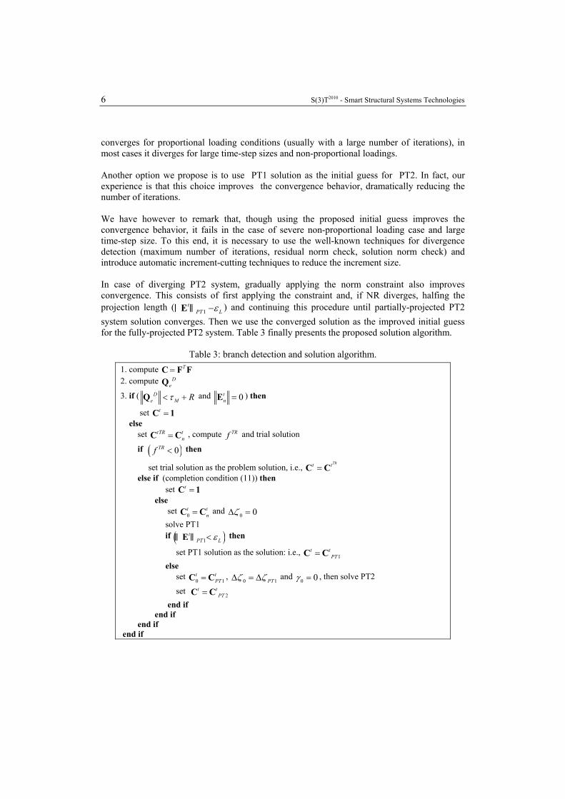
system solution converges. Then we use the converged solution as the improved initial guess for the fully-projected PT2 system. Table 3 finally presents the proposed solution algorithm.

Table 3: branch detection and solution algorithm. 1. compute T=C F F 2. compute D

eQ

3. if ( De M Rτ< +Q and 0t

n =E ) then

set t =C 1 else set tTR t

n=C C , compute TRf and trial solution

if ( )0TRf < then

set trial solution as the problem solution, i.e., TRt t=C C

else if (completion condition (11)) then set t =C 1 else set 0

t tn=C C and

0 0ζΔ = solve PT1 if ( )1

tPT Lε<E‖ ‖ then

set PT1 solution as the solution: i.e., 1t t

PT=C C else set

0 1t t

PT=C C , 0 1PTζ ζΔ = Δ and 0 0γ = , then solve PT2

set 2

t tPT=C C

end if end if end if end if


3. ALGORITHM ROBUSTNESS INVESTIGATION To investigate the robustness of the proposed integration algorithm as well as of the solution procedure, we simulate some benchmark tests at the Gauss point level. Up to now, different benchmark tests have been introduced in the literature; the paths are usually square-, butterfly-, triangle-, circle- or L-shaped, while they can be either strain- or stress-controlled. We simulate some uniaxial stress-controlled tension-compression tests. Afterward, a

11 22( )E E− -controlled butterfly-shaped and a 11 12( )E E− -controlled square-shaped path are simulated. In order to investigate the algorithm robustness, two different time-step sizes are adopted in each numerical test. Moreover, we report the average number of iterations in PT1 and PT2 for different selected cases to show the convergence behavior (as this information can somehow be related to the algorithm robustness). Averages are computed by dividing the total number of iterations in a test by the total number of calls to the corresponding subroutine. We also study the effects of using logarithmic mapping or exponential mapping as well as using a regularized scheme or Nucleation-Completion (NC) scheme. Following this procedure we consider four different cases: a regularized scheme with exponential mapping (exp+Reg), a nucleation-completion scheme with exponential mapping (exp+NC), a regularized scheme with logarithmic mapping (log+Reg) and a nucleation-completion scheme with logarithmic mapping (log+NC). Using this approach, it is possible to compare the local convergence behavior as well as the robustness of different algorithms. The reported result in this section are obtained using the unsymmetric model summarized in Table 3 of Part I. The following material properties, typical of NiTi [5], are adopted in all the simulations of this paper:

Table 4: Material parameters, typical of NiTi, used in the simulations [6]. parameter Value unit parameter value unit

E 51700 MPa εL 7.5 % ν 0.3 -- β 5.6 MPa ºC-1 h 750 MPa T0 -25 ºC R 140 MPa Af 0 ºC

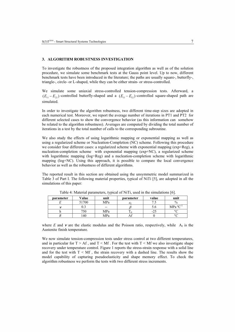
where E and ν are the elastic modulus and the Poisson ratio, respectively, while Af is the Austenite finish temperature. We now simulate tension-compression tests under stress control at two different temperatures, and in particular for T > Af , and T < Mf . For the test with T < Mf we also investigate shape recovery under temperature control. Figure 1 reports the stress-strain response with a solid line and for the test with T < Mf , the strain recovery with a dashed line. The results show the model capability of capturing pseudoelasticity and shape memory effect. To check the algorithm robustness we perform the tests with two different stress increments.


Table 5 shows the convergence results for different formulations in tension-compression tests. We use letters f and c to distinguish the results for the fine and coarse increments, respectively. For each case, a pair of numbers is reported corresponding to PT1 and PT2, respectively. As it is expected, using a NC scheme reduces the average number of iterations. It is interesting to note that using the logarithmic form reduces the number of iterations and this can be interpreted as the result of the reduced nonlinearity of the equations.

-10 -8 -6 -4 -2 0 2 4 6 8 10-1500

-1000

-500

0

500

1000

1500

E11

[ % ]

S11

[ M

Pa

]

T = 37° C

-8 -6 -4 -2 0 2 4 6 8

-600

-400

-200

0

200

400

600

E11

[ % ]

S11

[ M

Pa

]

T = -25° C

Figure 1: Uniaxial tension-compression test under stress control: T = 37ºC (left); T = 25ºC

(right). For T < Af strain recovery induced by heating is indicated with a dashed-dot line. Stress increment per step 15 MPa (line) and 150 MPa (circles).

Table 5: Convergence results for tension-compression tests. [6].

Exp+Reg Exp+NC Log+Reg Log+NC 6 7 4 4 37ºC(f) PT1

PT2 4 4 4 4 8 7 4 4 37ºC(c) PT1

PT2 4 4 4 4 6 5 4 4 -25ºC(f) PT1

PT2 4 4 4 4 5 4 4 4 37ºC(c) PT1

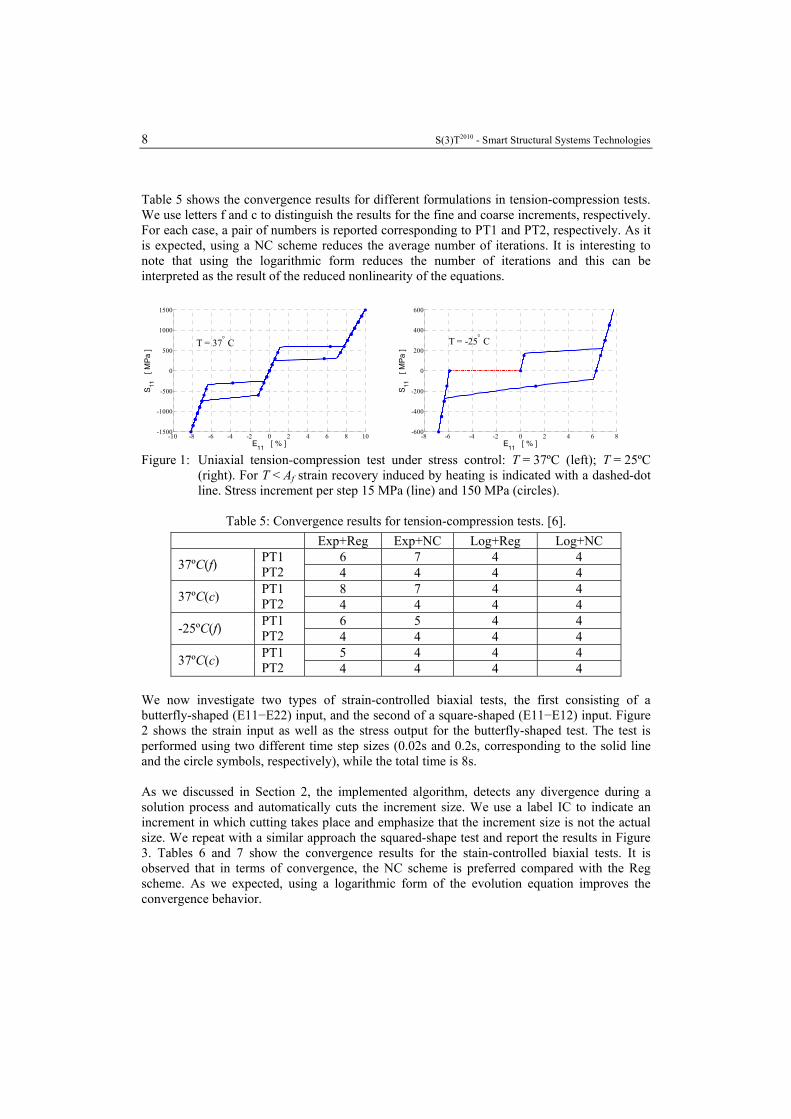
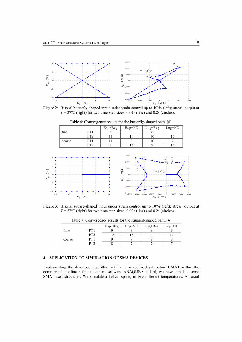
PT2 4 4 4 4 We now investigate two types of strain-controlled biaxial tests, the first consisting of a butterfly-shaped (E11−E22) input, and the second of a square-shaped (E11−E12) input. Figure 2 shows the strain input as well as the stress output for the butterfly-shaped test. The test is performed using two different time step sizes (0.02s and 0.2s, corresponding to the solid line and the circle symbols, respectively), while the total time is 8s. As we discussed in Section 2, the implemented algorithm, detects any divergence during a solution process and automatically cuts the increment size. We use a label IC to indicate an increment in which cutting takes place and emphasize that the increment size is not the actual size. We repeat with a similar approach the squared-shape test and report the results in Figure 3. Tables 6 and 7 show the convergence results for the stain-controlled biaxial tests. It is observed that in terms of convergence, the NC scheme is preferred compared with the Reg scheme. As we expected, using a logarithmic form of the evolution equation improves the convergence behavior.


-10 -5 0 5 10-10

-5

0

5

10

E11

[ % ]

E22

[ %

]

-6000 -4000 -2000 0 2000 4000 6000

-6000

-4000

-2000

0

2000

4000

6000

S11

[ MPa ]

S22

[ M

Pa

]

T = 37° C

IC

Figure 2: Biaxial butterfly-shaped input under strain control up to 10\% (left); stress output at

T = 37ºC (right) for two time step sizes: 0.02s (line) and 0.2s (circles).

Table 6: Convergence results for the butterfly-shaped path. [6]. Exp+Reg Exp+NC Log+Reg Log+NC

8 8 6 6 fine PT1 PT2 11 11 10 10

11 8 10 7 coarse PT1 PT2 9 10 9 10

-10 -5 0 5 10-10

-5

0

5

10

E11

[ % ]

E12

[ %

]

-5000 -4000 -3000 -2000 -1000 0 1000 2000 3000

-3000

-2000

-1000

0

1000

2000

3000

S11

[ MPa ]

S12

[ M

Pa

]

ICIC

ICIC

T = 37° C

Figure 3: Biaxial square-shaped input under strain control up to 10\% (left); stress output at

T = 37ºC (right) for two time step sizes: 0.02s (line) and 0.2s (circles).

Table 7: Convergence results for the squared-shaped path. [6] Exp+Reg Exp+NC Log+Reg Log+NC

9 9 8 8 Fine PT1 PT2 12 12 12 12

9 9 8 8 coarse PT1 PT2 8 7 7 7

4. APPLICATION TO SIMULATION OF SMA DEVICES Implementing the described algorithm within a user-defined subroutine UMAT within the commercial nonlinear finite element software ABAQUS/Standard, we now simulate some SMA-based structures. We simulate a helical spring in two different temperatures. An axial


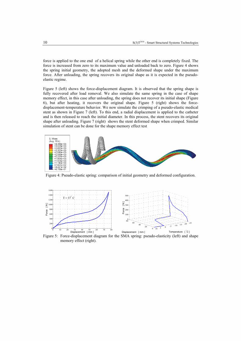
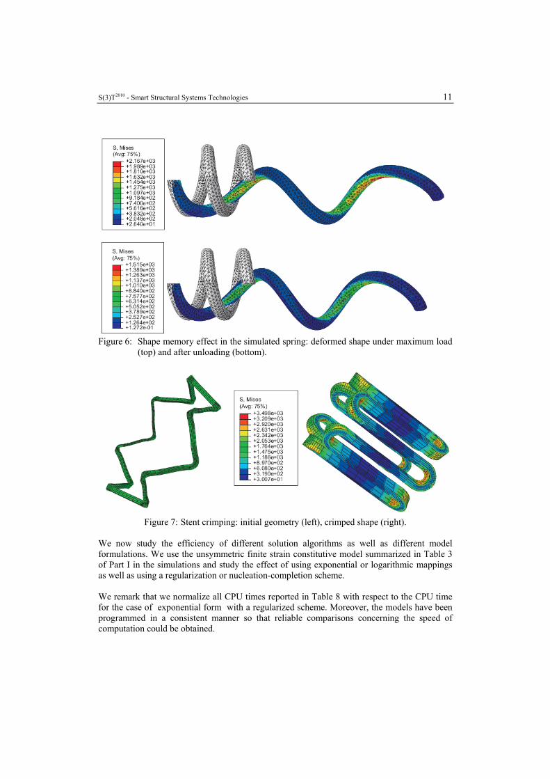
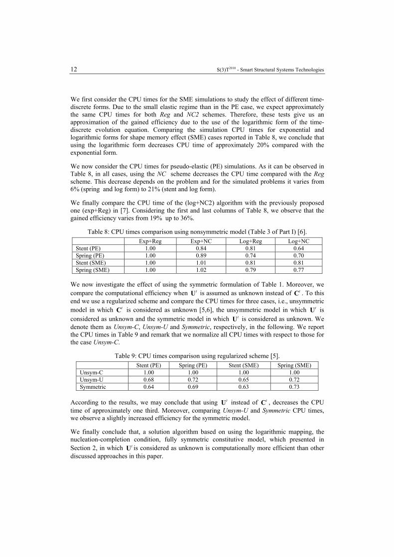
force is applied to the one end of a helical spring while the other end is completely fixed. The force is increased from zero to its maximum value and unloaded back to zero. Figure 4 shows the spring initial geometry, the adopted mesh and the deformed shape under the maximum force. After unloading, the spring recovers its original shape as it is expected in the pseudo-elastic regime. Figure 5 (left) shows the force-displacement diagram. It is observed that the spring shape is fully recovered after load removal. We also simulate the same spring in the case of shape memory effect, in this case after unloading, the spring does not recover its initial shape (Figure 6), but after heating, it recovers the original shape. Figure 5 (right) shows the force-displacement-temperature behavior. We now simulate the crimping of a pseudo-elastic medical stent as shown in Figure 7 (left). To this end, a radial displacement is applied to the catheter and is then released to reach the initial diameter. In this process, the stent recovers its original shape after unloading. Figure 7 (right) shows the stent deformed shape when crimped. Similar simulation of stent can be done for the shape memory effect test

Figure 4: Pseudo-elastic spring: comparison of initial geometry and deformed configuration.

0 10 20 30 40 50 60 70 800

200

400

600

800

1000

1200

1400

1600

Displacement [ mm ]

For

ce

[ N ]

T = 37° C

0

2040

6080

-25-20-15-10-50510

0

100

200

300

400

500

Temperature [ °C ]Displacement [ mm ]

For

ce

[ N ]

Figure 5: Force-displacement diagram for the SMA spring: pseudo-elasticity (left) and shape

memory effect (right).


Figure 6: Shape memory effect in the simulated spring: deformed shape under maximum load

(top) and after unloading (bottom).

Figure 7: Stent crimping: initial geometry (left), crimped shape (right).

We now study the efficiency of different solution algorithms as well as different model formulations. We use the unsymmetric finite strain constitutive model summarized in Table 3 of Part I in the simulations and study the effect of using exponential or logarithmic mappings as well as using a regularization or nucleation-completion scheme. We remark that we normalize all CPU times reported in Table 8 with respect to the CPU time for the case of exponential form with a regularized scheme. Moreover, the models have been programmed in a consistent manner so that reliable comparisons concerning the speed of computation could be obtained.


We first consider the CPU times for the SME simulations to study the effect of different time-discrete forms. Due to the small elastic regime than in the PE case, we expect approximately the same CPU times for both Reg and NC2 schemes. Therefore, these tests give us an approximation of the gained efficiency due to the use of the logarithmic form of the time-discrete evolution equation. Comparing the simulation CPU times for exponential and logarithmic forms for shape memory effect (SME) cases reported in Table 8, we conclude that using the logarithmic form decreases CPU time of approximately 20% compared with the exponential form. We now consider the CPU times for pseudo-elastic (PE) simulations. As it can be observed in Table 8, in all cases, using the NC scheme decreases the CPU time compared with the Reg scheme. This decrease depends on the problem and for the simulated problems it varies from 6% (spring and log form) to 21% (stent and log form). We finally compare the CPU time of the (log+NC2) algorithm with the previously proposed one (exp+Reg) in [7]. Considering the first and last columns of Table 8, we observe that the gained efficiency varies from 19% up to 36%.

Table 8: CPU times comparison using nonsymmetric model (Table 3 of Part I) [6]. Exp+Reg Exp+NC Log+Reg Log+NC

Stent (PE) 1.00 0.84 0.81 0.64 Spring (PE) 1.00 0.89 0.74 0.70 Stent (SME) 1.00 1.01 0.81 0.81 Spring (SME) 1.00 1.02 0.79 0.77

We now investigate the effect of using the symmetric formulation of Table 1. Moreover, we compare the computational efficiency when tU is assumed as unknown instead of tC . To this end we use a regularized scheme and compare the CPU times for three cases, i.e., unsymmetric model in which tC is considered as unknown [5,6], the unsymmetric model in which tU is considered as unknown and the symmetric model in which tU is considered as unknown. We denote them as Unsym-C, Unsym-U and Symmetric, respectively, in the following. We report the CPU times in Table 9 and remark that we normalize all CPU times with respect to those for the case Unsym-C.

Table 9: CPU times comparison using regularized scheme [5]. Stent (PE) Spring (PE) Stent (SME) Spring (SME)

Unsym-C 1.00 1.00 1.00 1.00 Unsym-U 0.68 0.72 0.65 0.72 Symmetric 0.64 0.69 0.63 0.73

According to the results, we may conclude that using tU instead of tC , decreases the CPU time of approximately one third. Moreover, comparing Unsym-U and Symmetric CPU times, we observe a slightly increased efficiency for the symmetric model. We finally conclude that, a solution algorithm based on using the logarithmic mapping, the nucleation-completion condition, fully symmetric constitutive model, which presented in Section 2, in which tU is considered as unknown is computationally more efficient than other discussed approaches in this paper.


REFERENCES [1] Souza, A.C. et al.– “Three-dimensional model for solids undergoing stress-induced phase

transformations”. European Journal of Mechanics A/Solids 17 (5), 789–806, 1998. [2] Auricchio, F., Petrini, L. – “Improvements and algorithmical considerations on a recent

three-dimensional model describing stress-induced solid phase transformations”. International Journal for Numerical Methods in Engineering 55, 1255 – 1284, 2002.

[3] Auricchio, F., Petrini, L. – “A three-dimensional model describing stress-temperature induced solid phase transformations: thermomechanical coupling and hybrid composite applications”. International Journal for Numerical Methods in Engineering 61 (5), 716–737, 2004.

[4] Auricchio, F., Petrini, L. – “A three-dimensional model describing stress-temperature induced solid phase transformations: solution algorithm and boundary value problems”. International Journal for Numerical Methods in Engineering 61, 807 – 836, 2004.

[5] Arghavani, J., et al. – “An improved, fully symmetric, finite strain phenomenological constitutive model for shape memory alloys”. Comp. Mat. Sci., submitted.

[6] Arghavani, J., et al. – “On the robustness and efficiency of integration algorithms for a 3D finite strain SMA constitutive model”. Int. J. Num. Meth. Eng., submitted.

[7] Evangelista, et al.– “A 3D SMA constitutive model in the framework of finite strain”. International Journal for Numerical Methods in Engineering, 2009.

[8] Christ, D., Reese, S. – “A finite element model for shape memory alloys considering thermomechanical couplings at large strains”. International Journal of Solids and Structures 46 (20), 3694–3709, 2009.

[9] Reese, S., Christ, D. – “Finite deformation pseudo-elasticity of shape memory alloys –constitutive modelling and finite element implementation”. International Journal of Plasticity 24 (3), 455–482, 2008.

Documents

ON THE CONSTITUTIVE MODELING AND NUMERICAL … · Kuhn-Tucker conditions: ff≤≥ =0, 0, 0ζζ&& Norm operator: ‖QQQD‖= DD: We now treat the nonlinear problem summarized in Table