On the cavity model for solvent shifts of excited states — a critical appraisal

Journal of Molecular Structure (Theo&em), 216 (1992) 279-297 Elsevier Science Publishers B.V.. Amsterdam

219

On the cavity model for - a critical appraisal

Thomas Fox and Notker Rosch

solvent shifts of excited states

Lehrstuhl fiir Theoretische Chemie, Technische Universitiit Miinchen, W-8046 Garching (Germany)

(Received 31 January 1992)

Abstract

We present model investigations on the solvatochromic shift of several organic molecules. The excitation energies are calculated within the INDO/SCI approach; solvent effects are taken into account self-consistently via a cavity model. A cavity of arbitrary shape is admitted, the corresponding surface charge density being represented by a finite number of point charges. Applying the model at different levels of sophistication, we investigate the effect of the point density on the accuracy of the results and we suggest a method of monitoring their quality. The evaluation of the electronic excitation energies in different solvents demonstrates the partial success of currently used electrostatic cavity methods for modeling solvatochromic shifts of electronic absorptions, but also their inherent deficiencies. Some strategies for improvement of purely electrostatic cavity models are discussed.

INTRODUCTION

In recent years much effort has been directed toward elucidating the effects of solvation on molecular properties. Besides extensive experimental investigations [1,2] many theoretical studies have been concerned with modeling the interactions in solute-solvent systems, mostly for ground state energetics [3,4]. Various strategies have been pursued for modeling such solvent effects, using a quantum mechanical description of the solute. One possibility is to use a discrete representation of the solvent, i.e. to surround the molecule of interest by a finite number of solvent molecules in a fixed geometry (see, for example, refs 5-8); sometimes even a minimal- istic approach with only one solvent molecule is employed [6]. These investigations provide valuable information because they probe specific directed

Correspondence to: N. Riisch, Lehrstuhl fiir Theoretische Chemie, Technische Universitlit Munchen, W-8046 Garching, Germany; tel. ( + + 49 + 89) 3209 3616; fax ( + + 49 + 89) 3209 3622; E-mail [email protected].

0166-1280/92/$05.00 0 1992 Elsevier Science Publishers B.V. All rights reserved.

280 T. Fox, N. RtischlJ. Mol. Strut. (Theo&em) 276 (1992) 27g297

interactions between the solvent and the solute [9,10]. In recent years, with the ever increasing power of computers, many attempts have been made to obtain a statistical description of solute-solvent systems with classical potentials and molecular dynamics methods [ll-131. Nevertheless, these molecular dynamics methods still require enormous computational resour- ces and are therefore often not yet practicable for larger systems.

A continuum formalism provides a partly complementary approach to this fully microscopic strategy. In such a procedure a solute molecule is described quantum mechanically, but the model is augmented by a continuum model description of the surrounding solvent [4]. Here, the attempt is to make the effect of the medium into an effective operator modifying the original Hamiltonian of the solute. Examples are provided by the solvaton concept (in which an imaginary particle represents the oriented solvent distribution around each atom [14-161) and various cavity models [9,17-221. The latter models have enjoyed some popularity: they have been used to investigate (among others) solvation energies [20], conformational equi- libria [20,23], and solvent modulation of electron transfer processes [24] and chemical reaction mechanisms [25]. However, although many investigations have been concerned with understanding molecular ground state properties of solvated molecules, only rather limited experience is available yet for the calculation of electronic excitations in solution, especially in the UV-visible region [9,26-281.

In this paper we report the use of a cavity model that admits a realistic cavity shape for calculating solvatochromic shifts of organic molecules. The excitation energies are calculated in the INDO/S-CI approach [29,30]. In a previous study [lo] we applied this model to the n-x* transition of acetone and found that the relative shifts between different solvents can be reproduced satisfactorily. Here we give a more detailed account by extend- ing the investigation to other molecules and we discuss some of the problems that arise when cavity models are applied to calculating electronic absorption spectra in solution. After a brief review of some current implementations, we describe various aspects of the cavity model, e.g. problems connected to the discretization of the continuum model and to the implementation in the INDO method. Finally, we present results that illustrate both the accomplishments and the difficulties that one encounters when a physically realistic cavity is used in the calculation of the electronic spectra of solvated molecules.

IMPLEMENTATIONS OF CAVITY MODELS

All cavity models seek to combine a detailed quantum mechanical description of the solute with a model of the surrounding solvent. The solvent is modeled as an infinite continuous medium that is characterized by some

T. Fox, N. R&h/J. Mol. Struct. (Theo&em) 276 (1992) 279-297 281

macroscopic properties and the solute molecule is placed in a cavity prepared in this medium [17,18]; the interaction between solute and solvent is taken into account in an averaged (and/or approximated) way.

The total solvent effect consists of long-range electrostatic as well as short-range dispersion, repulsion and cavitation contributions [l]. Further- more, directed covalent solute-solvent interactions may require treating some solvent molecules explicitly inside the cavity [9,10]. For certain investigations it may be sufficient to consider only the electrostatic part, although the other contributions may be of considerable size. As a consequence, most implementations of cavity models are only concerned with electrostatic interactions; few studies so far have taken other contributions into account [31,32]. Especially for the investigation of electronic excitations in which the electronic properties of the molecule may change appreciably, it is commonly assumed that it suffices to take the long-range electrostatic interaction into account. Therefore, almost all investigations which have attempted to model solvatochromic shifts have been restricted to the electrostatic contribution [9,33].

For the calculation of this electrostatic part of the solvation energy the surrounding medium is modeled as a dielectric continuum in which the charge distribution of the embedded molecule induces a polarization charge density. This polarization sets up a response field or reaction field, which in turn acts back upon the molecule. The interaction of this reaction field with the charge distribution computed for the isolated molecule may serve as a first estimate of the solvent effect [17,33]. To arrive at a higher order description of the interaction the resulting reaction field in the solute Hamiltonian must be included in a self-consistent manner [20,22,34].

Most previous implementations of the cavity models use a spherical cavity because for this cavity shape an analytical solution of the reaction potential is available [17]. The only parameter of this approach is the cavity radius, which has been estimated by a variety of methods [l&20,24,35]. Especially for solute molecules or clusters of molecules whose shape is far from spherical, the description of the cavity by a sphere (implying only one parameter) seems questionable. At this point it is worth noting that, in all the implementations discussed so far, the cavity itself has no direct physical reality. It is merely an auxiliary tool for evaluating the electrostatic potential and it enters the formalism only implicitly via its effective size. The cavity radius (a reasonable physical concept for spherical molecules) becomes more and more ill-defined for arbitrarily shaped solutes and thus becomes a mere parameter in the calculation of the solvent effect, able to be adjusted to reproduce experimental data. Owing to this nature, very small cavities even to the extent that parts of the molecules lie outside the “cavity” do not pose any formal problems for the calculation of the solvent effect, because only effective interactions are evaluated [9].

282 T. For, N. R&h/J. Mol. &r&et. (T~~~rn~ 276 (1992) 279-297

No matter how the cavity radius is determined, there always remains some uncertainty, which is then amplified in the resulting solvent effect by the nature of the reaction field formulae: the dipole contribution depends on the third power of the radius a,; the contribution of the Ith moment depends on af ’ ’ . There have been attempts to improve the models by using other suitable constant coordinate surfaces (e.g. ellipsoids) which allow a more realistic cavity shape while still affording an analytical solution [23]. However, this complication of the formalism introduces additional parameters whose choice may again pose a problem.

A different strategy, avoiding unphysical shape restrictions on the cavity, is followed by implementations which describe the solute volume as a system of interlocking spheres [21] or by a smooth solvent-accessible surface [36,37]. In this way, molecules of arbitrarily complicated shape may be treated, e.g. macromolecules or supermolecules which consist of the solute and some selected solvent molecules. However, no analytical solution of the reaction field is available for such cavities and one has to resort to a numerical procedure. Two alternatives are available for obtain- ing the reaction field via a solution of Poisson’s equation. The first employs a finite difference algorithm on a three-dimensional grid [38,39]; the second reduces the calculation of the volume integrals to the determination of a two-d~ensional polarization charge density located on the cavity surface 221,371. This charge density is then used directly to determine the necessary modification of the solute Hamiltonian. The latter approach has been implemented at two levels of numerical sophistication. One procedure combines an analytical description of the cavity surface with a numerical evaluation of the occurring surface integrals [37,40,41] to determine this surface charge density; the other has been implemented by us within the INDO/S-CI model [29,30] and is described in the following section.

The study of the solvent effects on electronic absorption spectra has been an area of interest for a long time [1,2]. Much work has been done to understand the factors that determine the red or blue shift in the spectra of organic molecules immersed in different solvents E&2]. Based on the Kirkwood-Onsager reaction field model, a theory has been formulated that connects the dipole moments of the ground and excited states with the observed solvent shift of the absorption bands [33]. This model uses the free (vacuum) molecular values, neglecting any modifications of the solute due to the reaction field. Recently, a method has been suggested that incor- porates the dipole term of the reaction field into the solute hamiltonian in a self-consistent way [9]. More sophisticated methods which also take higher moments of the charge distribution into account are also available [26,42].

All these methods share the model of a spherical cavity so the objections stated above apply to them all. Therefore, it seemed interesting to use a

T. Fox, N. Riisch/J. Mol. Strut. (Theo&m) 276 (1992) 279-297 283

model which allows a more realistic cavity shape and to apply it to the solvatochromic shifts of molecular electronic transitions. Previous applica- tions have shown that the model is, in principle, able to account for solvatochromic shifts of small organic molecules [43,44]. However, few attempts have been made so far to investigate larger molecules or the differential effects of various solvents. In the following we study the cavity model for excited states in greater detail.

COMPUTATIONAL DETAILS

Ground state calculations

A basic feature of the present solvatization model is the polarization charge density g located on the cavity surface. This charge density c(r), which gives rise to an additional potential energy term v[o] in the solute Hamiltonian, can be obtained by

o(r) = &a0 )L - ZIP + d(r) (1) where Elr) is the electric field due to the total electrostatic potential V(r) and n-(r) is the outside normal of the cavity surface. The scaling factor

g(E) = (& - l) 4?c&

depends on the (static) macroscopic dielectric constant of the solvent eO. It should be noted that V(r) consists of both the electrostatic potential v[p] of the charge distribution p of the solute and the potential V[a] due to the surface charge density.

To perform the necessary numerical calculations, the cavity surface is divided into small patches. Within each such patch (of area ASi) the surface charge o(r) is assumed to be constant and is represented by a point charge qi = o(ri)ASi. 0 ne then applies the following computational procedure.

(1) The cavity surface is defined and the positions of the point charges ri and the accompanying patch sizes ASi are determined. Deviating from the original method [Zl], we describe the surface of the solute molecule by Connolly’s concept of the “solvent accessible surface” [36]. This surface is defined essentially by rolling a sphere (representing a typical atom of a solute molecule) on the surface defined by the interlocking atomic spheres of the molecule. It therefore consists of convex and concave sections and avoids sharp edges or grooves. The exposed parts of the sphere surfaces are covered by a net of circles of latitude and longitude. The resulting set of nodes is triangulated [45] to achieve a smoother convergence. In this way, a consistent partitioning of the molecular surface is generated. Ultimately, each of the resulting triangles is taken to define a patch, at the midpoint of which a point charge is located.

284 T. Fox, N. RBschlJ. Mol. Strut. (Theo&em) 276 (1992) 279-297

(2) The initial surface charge density o” due to the electrostatic field E[p”] set up by the free solute molecule is calculated:

In our implementation the charge density of the solute is represented by a set of point charges obtained by a Mulliken population analysis and located at the atomic centers. This is obviously a rather simple approximation [4,46,47], especially for electrostatic calculations. We therefore tested its validity by using a more accurate representation of the molecular electrostatic potential (see approximation II in ref. 47):

Calculations with this representation showed the same general trends as those with Mulliken point charges, but the solvent effects were somewhat reduced in size. However, for small atomic spheres the more accurate calculation of the molecular electrostatic potential led to a considerable excess charge in the nearby cavity surface region and to numerical insta- bilities. Therefore, we decided to retain, as a first approximation, the Mulliken charges.

(3) An iterative calculation of point charges is performed until v[P”k

(7 = g(Eo)6* (E~pO] + E$Y-‘1)

(4) A new V[a] is calculated

the mutual polarization of the surface self-consistency is reached for a given

and a new SCF calculation with the improved Hamiltonian is started, resulting in a new molecular charge density pl. Note that the factor of one half is a consequence of the induced nature of the surface charge density. (For an alternative view see refs. 3 and 9). Consistent with the INDO method the calculation of the matrix elements of v[o] involves no three- center or four-center integrals.

(5) Steps 3 and 4 are repeated until self-consistency is reached. Further details of the original method can be found elsewhere [21].

Electronic excited states

The computational scheme sketched above for the ground state can be adapted to calculate the influence of the solvent on electronic absorption processes [48]. To this end, the response of the solvent to changes in the

T. Fox, N. RiischlJ. Mol. Strut. (Theo&em) 276 (1992) 279-297 285

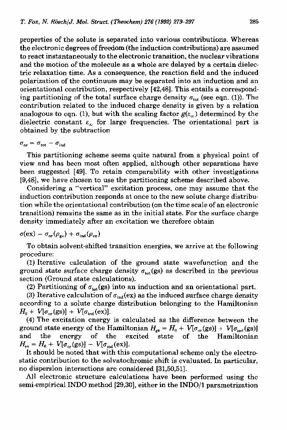
properties of the solute is separated into various contributions. Whereas the electronic degrees of freedom (the induction contributions) are assumed to react instantaneously to the electronic transition, the nuclear vibrations and the motion of the molecule as a whole are delayed by a certain dielectric relaxation time. As a consequence, the reaction field and the induced polarization of the continuum may be separated into an induction and an orientational contribution, respectively [42,48]. This entails a corresponding partitioning of the total surface charge density o,,, (see eqn. (1)). The contribution related to the induced charge density is given by a relation analogous to eqn. (l), but with the scaling factor g(s,) determined by the dielectric constant E, for large frequencies. The orientational part is obtained by the subtraction

(T or = ctot - Oind

This partitioning scheme seems quite natural from a physical point of view and has been most often applied, although other separations have been suggested [49]. To retain comparability with other investigations [9,48], we have chosen to use the partitioning scheme described above.

Considering a “vertical” excitation process, one may assume that the induction contribution responds at once to the new solute charge distribution while the orientational contribution (on the time scale of an electronic transition) remains the same as in the initial state. For the surface charge density immediately after an excitation we therefore obtain

o(ex) = car (Pgs) + Oind (Pa)

To obtain solvent-shifted transition energies, we arrive at the following procedure:

(1) Iterative calculation of the ground state wavefunction and the ground state surface charge density crt,,,(gs) as described in the previous section (Ground state calculations).

(2) Partitioning of a,,(gs) into an induction and an orientational part. (3) Iterative calculation of Uind(ex) as the induced surface charge density

according to a solute charge distribution belonging to the Hamiltonian Ho + v[OO,(gs)] + flO.ind tex)l.

(4) The excitation energy is calculated as the difference between the ground state energy of the Hamiltonian H,, = H, + V[a,,(gs)] + uoind(gs)] and the energy of the excited state of the Hamiltonian N,, = & + qcor (fP)l + V[Oind WI.

It should be noted that with this computational scheme only the electrostatic contribution to the solvatochromic shift is evaluated. In particular, no dispersion interactions are considered [31,50,51].

All electronic structure calculations have been performed using the semi-empirical INDO method [29,30], either in the INDO/ parametrization

286 T. Fox, N. ~~schl~. ~01. Stmct. (~~~he~) 276 (1992) 27S297

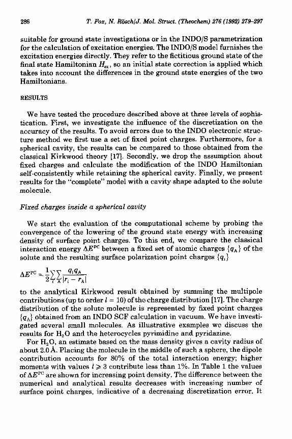
suitable for ground state investigations or in the INDO/S parametrization for the calculation of excitation energies. The INDO/S model furnishes the excitation energies directly. They refer to the fictitious ground state of the final state Hamiltonian H, , so an initial state correction is applied which takes into account the differences in the ground state energies of the two Hamiltonians.

RESULTS

We have tested the procedure described above at three levels of sophistication. First, we investigate the influence of the discretization on the accuracy of the results. To avoid errors due to the INDO electronic structure method we first use a set of fixed point charges. Furthermore, for a spherical cavity, the results can be compared to those obtained from the classical Kirkwood theory [17]. Secondly, we drop the assumption about fixed charges and calculate the modification of the INDO Hamiltonian self-consistently while retaining the spherical cavity. Finally, we present results for the “complete” model with a cavity shape adapted to the solute molecule.

Fixed changes inside a spherical cavity

We start the evaluation of the computational scheme by probing the convergence of the lowering of the ground state energy with increasing density of surface point charges. To this end, we compare the classical interaction energy AbEFC between a fixed set of atomic charges (qA) of the solute and the resulting surface polarization point charges {qi)

to the analytical Kirkwood result obtained by summing the multipole contributions (up to order I = 10) of the charge distribution [l?]. The charge distribution of the solute molecule is represented by fixed point charges {qA} obtained from an INDO SCF calculation in vacuum. We have investigated several small molecules. As illustrative examples we discuss the results for H,O and the heterocycles pyrimidine and pyridazine.

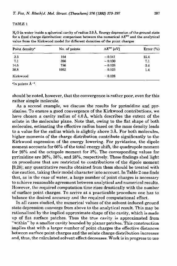
For H,O, an estimate based on the mass density gives a cavity radius of about 2.0 A. Placing the molecule in the middle of such a sphere, the dipole contribution accounts for 80% of the total interaction energy; higher moments with values I 2 3 contribute less than 1%. In Table 1 the values of AEPC are shown for increasing point density. The difference between the numerical and analytical results decreases with increasing number of surface point charges, indicative of a decreasing discretization error. It

T. Fox, N. RGschlJ. Mol. Struct. (Theo&em) 276 (1992) 27$297 287

TABLE 1

H,O in water inside a spherical cavity of radius 2.0A. Energy depression of the ground state for a fixed charge distribution: comparison between the numerical AEPC and the analytical value from the Kirkwood model for different densities of the point charges

Point density” No. of points AEPC [eV] Error (%)

3.3 7.1

14.5 38.8

Kirkwood

“In points A-“.

164 - 0.141 15.4 356 - 0.130 7.1 736 - 0.126 3.4

1952 - 0.123 1.4

- 0.128

should be noted, however, that the convergence is rather poor, even for this rather simple molecule.

As a second example, we discuss the results for pyrimidine and pyridazine. To ensure a good convergence of the Kirkwood contributions, we have chosen a cavity radius of 4.0& which describes the extent of the solute in the molecular plane. Note that, owing to the flat shape of both molecules, estimating the effective radius based on the mass density leads to a value for the radius which is slightly above 3A. For both molecules, higher moments of the charge distribution contribute significantly to the Kirkwood expression of the energy lowering. For pyridazine, the dipole moment accounts for 66% of the total energy shift, the quadrupole moment for 26% and the octopole moment for 3%. The corresponding values for pyrimidine are 26%, 38%, and 28%, respectively. These findings shed light on procedures that are restricted to contributions of the dipole moment [9,28]; any quantitative results obtained from them should be treated with due caution, taking their model character into account. In Table 2 one finds that, as in the case of water, a large number of point charges is necessary to achieve reasonable agreement between analytical and numerical results. However, the required computation time rises drastically with the number of surface point charges. To arrive at a practicable procedure one has to balance the desired accuracy and the required computational effort.

In all cases studied, the numerical values of the solvent-induced ground state depression converge from above to the analytical result. This may be rationalized by the implied approximate shape of the cavity, which is made up of flat surface patches. Thus the true cavity is approximated from “within” by a smaller cavity bounded by planar patches. This construction implies that with a larger number of point charges the effective distances between surface point charges and the solute charge distribution increases and, thus, the calculated solvent effect decreases. Work is in progress to use

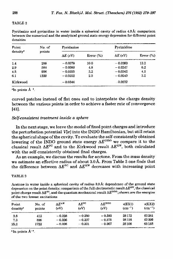
TABLE 2

Pyridaaine and pyrimidine in water inside a spherical cavity of radius 4.QA: comparison between the numerical and the analytical ground state energy depression fox different point densities

Point density”

No. of points

Pyridazine

AE (eV) Error (%)

Pyrimidine

AE (eV) Error (%)

1.4 288 - 0.6373 10.0 - 9.0263 13.2 2.9 584 - 6.9369 4.6 - 9.0247 6.2 4.5 968 - 0.0356 3.2 - 0.0242 4.2 6.1 1220 - 0.0352 2.5 - 0.0240 3.2

Kirkwood - 0.0344 - 0.0232

“In points A-‘.

curved patches instead of flat ones and to interpolate the charge density between the various points in order to achieve a faster rate of convergence

[411.

In the next stage, we leave the model of fixed point charges and introduce the perturbation potential I+] into the INDO Hamiltonian, but still retain the spherical shape of the cavity. To evaluate the self-consistently obtained lowering of the INDO ground state energy AEINDo we compare it to the classical result AEPC and to the Kirkwood result AEKW, both calculated with the self-consistently obtained final charges.

As an example, we discuss the results for acetone. From the mass density we estimate an effective radius of about 3.OA. From Table 3 one finds that the difference between AEPC and AE KW decreases with increasing point

TABLE 3

Acetone in water inside a spherical cavity of radius 3.OA: dependence of the ground state depression on the point density; comparison of the full electrostatic result AEKW, the classical point charge result AEPC, and the quantum mechanical result AEINW; shown are the energies of the two lowest excitations

Point No. of density” points

3.6 412 7.3 826

15.2 1722

A.@= (eV)

- 0.328 - 0.326 - 0.326

PC

&

- 0.350 - 0.337 - 6.331

AE’N@u (eV)

- 0.393 - 0.375 - 0.367

V(EX1) r{EX2) (cm--‘) (cm-l)

28172 63 261 28 128 63 269 28 106 63 183

“In points A-“.

T. Fox, N. RiischjJ. Mol. Struct. (Theochem) 276 (1992) 27>297 289

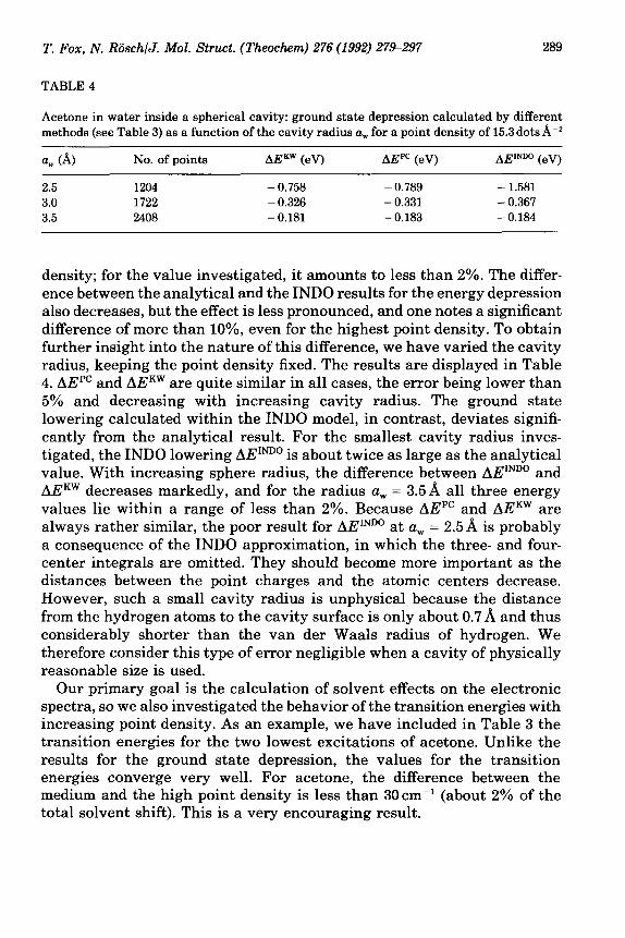
TABLE 4

Acetone in water inside a spherical cavity: ground state depression calculated by different methods (see Table 3) as a function of the cavity radius a.,, for a point density of 15.3 dots k”

a, (A)

2.5 3.0 3.5

No. of points

1204 1722 2408

AEKW (eV)

- 0.758 - 0.326 - 0.181

AEPC (eV)

- 0.789 - 0.331 - 0.183

AEINDo (eV)

- 1.581 - 0.367 - 0.184

density; for the value investigated, it amounts to less than 2%. The difference between the analytical and the INDO results for the energy depression also decreases, but the effect is less pronounced, and one notes a significant difference of more than lo%, even for the highest point density. To obtain further insight into the nature of this difference, we have varied the cavity radius, keeping the point density fixed. The results are displayed in Table 4. AEPC and AEKW are quite similar in all cases, the error being lower than 5% and decreasing with increasing cavity radius. The ground state lowering calculated within the INDO model, in contrast, deviates significantly from the analytical result. For the smallest cavity radius investigated, the INDO lowering AErNDo is about twice as large as the analytical value. With increasing sphere radius, the difference between AEINDo and AEKW decreases markedly, and for the radius a, = 3.5A all three energy values lie within a range of less than 2%. Because AEPC and AEKW are always rather similar, the poor result for AEINDo at a, = 2.5A is probably a consequence of the INDO approximation, in which the three- and four- center integrals are omitted. They should become more important as the distances between the point charges and the atomic centers decrease. However, such a small cavity radius is unphysical because the distance from the hydrogen atoms to the cavity surface is only about 0.7 A and thus considerably shorter than the van der Waals radius of hydrogen. We therefore consider this type of error negligible when a cavity of physically reasonable size is used.

Our primary goal is the calculation of solvent effects on the electronic spectra, so we also investigated the behavior of the transition energies with increasing point density. As an example, we have included in Table 3 the transition energies for the two lowest excitations of acetone. Unlike the results for the ground state depression, the values for the transition energies converge very well. For acetone, the difference between the medium and the high point density is less than 30cm-’ (about 2% of the total solvent shift). This is a very encouraging result.

290 T. Fox, N. RiischlJ. Mol. Struct. (Theo&em) 276 (1992) 27S297

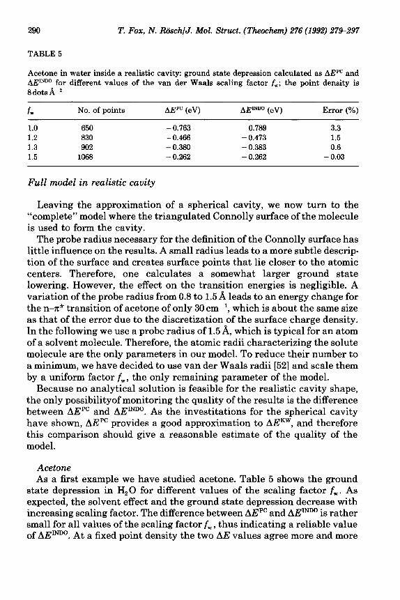
TABLE 5

Acetone in water inside a realistic cavity: ground state depression calculated as AEPC and AEINDo for different values of the van der Waals scaling factor f,; the point density is 8dotsk’

fw No. of points AEPC (eV) AEINDo (eV) Error (%)

1.0 650 - 0.763 - 0.789 3.3 1.2 830 - 0.466 - 0.473 1.5 1.3 902 - 0.380 - 0.383 0.6 1.5 1068 - 0.262 - 0.262 - 0.03

Full model in realistic cavity

Leaving the approximation of a spherical cavity, we now turn to the “complete” model where the triangulated Connolly surface of the molecule is used to form the cavity.

The probe radius necessary for the definition of the Connolly surface has little influence on the results. A small radius leads to a more subtle description of the surface and creates surface points that lie closer to the atomic centers. Therefore, one calculates a somewhat larger ground state lowering. However, the effect on the transition energies is negligible. A variation of the probe radius from 0.8 to 1.5 A leads to an energy change for the n-x* transition of acetone of only 30 cm-‘, which is about the same size as that of the error due to the discretization of the surface charge density. In the following we use a probe radius of 1.5 A, which is typical for an atom of a solvent molecule. Therefore, the atomic radii characterizing the solute molecule are the only parameters in our model. To reduce their number to a minimum, we have decided to use van der Waals radii [52] and scale them by a uniform factor f,, the only remaining parameter of the model.

Because no analytical solution is feasible for the realistic cavity shape, the only possibilityof monitoring the quality of the results is the difference between AEPC and AEiNDo. As the investitations for the spherical cavity have shown, AEPC provides a good approximation to AEKW, and therefore this comparison should give a reasonable estimate of the quality of the model.

Acetone As a first example we have studied acetone. Table 5 shows the ground

state depression in H,O for different values of the scaling factor f,. As expected, the solvent effect and the ground state depression decrease with increasing scaling factor. The difference between AEPC and AEiNDo is rather small for all values of the scaling factor f,, thus indicating a reliable value of AErNDo. At a fixed point density the two AE values agree more and more

T. Fox, N. Riisch/J. Mol. Struct. (Theo&em) 276 (1992) 27%297 291

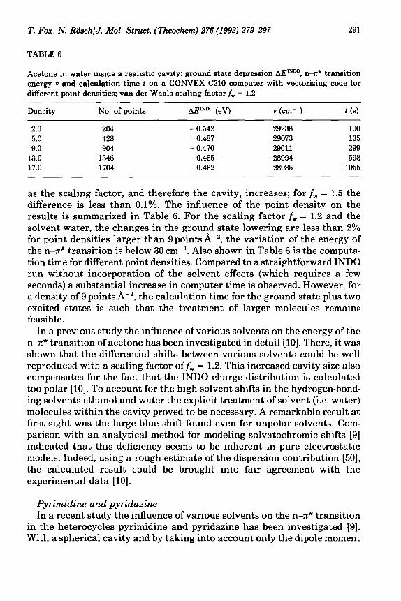
TABLE 6

Acetone in water inside a realistic cavity: ground state depression AE’-, n-z* transition energy v and calculation time t on a CONVEX C210 computer with vectorizing code for different point densities; van der Waals scaling factor f, = 1.2

Density No. of points AE’- (eV) v (cm-‘) t (s)

2.0 204 - 0.542 29238 100 5.0 428 - 0.487 29073 135 9.0 904 - 0.470 29011 299

13.0 1346 - 0.465 28994 598 17.0 1704 - 0.462 28985 1055

as the scaling factor, and therefore the cavity, increases; for f, = 1.5 the difference is less than 0.1%. The influence of the point density on the results is summarized in Table 6. For the scaling factor f, = 1.2 and the solvent water, the changes in the ground state lowering are less than 2% for point densities larger than 9 points A-‘, the variation of the energy of the n-n* transition is below 30 cm ‘. Also shown in Table 6 is the computation time for different point densities. Compared to a straightforward INDO run without incorporation of the solvent effects (which requires a few seconds) a substantial increase in computer time is observed. However, for a density of 9 points A-‘, the calculation time for the ground state plus two excited states is such that the treatment of larger molecules remains feasible.

In a previous study the influence of various solvents on the energy of the n-x* transition of acetone has been investigated in detail [lo]. There, it was shown that the differential shifts between various solvents could be well reproduced with a scaling factor off, = 1.2. This increased cavity size also compensates for the fact that the INDO charge distribution is calculated too polar [lo]. To account for the high solvent shifts in the hydrogen-bonding solvents ethanol and water the explicit treatment of solvent (i.e. water) molecules within the cavity proved to be necessary. A remarkable result at first sight was the large blue shift found even for unpolar solvents. Com- parison with an analytical method for modeling solvatochromic shifts [9] indicated that this deficiency seems to be inherent in pure electrostatic models. Indeed, using a rough estimate of the dispersion contribution [50], the calculated result could be brought into fair agreement with the experimental data [lo].

Pyrimidine and pyridazine In a recent study the influence of various solvents on the n-x* transition

in the heterocycles pyrimidine and pyridazine has been investigated [9]. With a spherical cavity and by taking into account only the dipole moment

292 T. Fox, N. RiischlJ. Mol. Struct. (Theochem) 276 (1992) 27%297

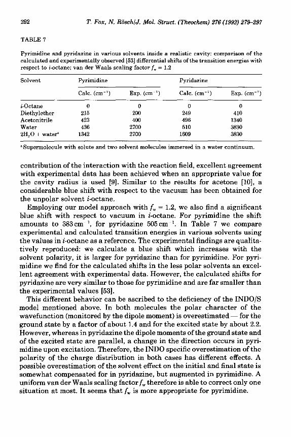
TABLE 7

Pyrimidine and pyridazine in various solvents inside a realistic cavity: comparison of the calculated and experimentally observed [53] differential shifts of the transition energies with respect to i-octane; van der Waals scaling factor f, = 1.2

Solvent Pyrimidine

Calc. (cm-‘) Exp. (cm-‘)

Pyridazine

Calc. (cm-‘) Exp. (cm-‘)

i-Octane 0 0 0 0 Diethylether 215 200 249 410 Acetonitrile 423 400 496 1340 Water 436 2700 510 3830 2H,O + water” 1342 2700 1609 3830

“Supermolecule with solute and two solvent molecules immersed in a water continuum.

contribution of the interaction with the reaction field, excellent agreement with experimental data has been achieved when an appropriate value for the cavity radius is used [9]. Similar to the results for acetone [lo], a considerable blue shift with respect to the vacuum has been obtained for the unpolar solvent i-octane.

Employing our model approach with f, = 1.2, we also find a significant blue shift with respect to vacuum in i-octane. For pyrimidine the shift amounts to 383cm-‘, for pyridazine 505 cm-‘. In Table 7 we compare experimental and calculated transition energies in various solvents using the values in i-octane as a reference. The experimental findings are qualitatively reproduced: we calculate a blue shift which increases with the solvent polarity, it is larger for pyridazine than for pyrimidine. For pyrimidine we find for the calculated shifts in the less polar solvents an excellent agreement with experimental data. However, the calculated shifts for pyridazine are very similar to those for pyrimidine and are far smaller than the experimental values [53].

This different behavior can be ascribed to the deficiency of the INDO/S model mentioned above. In both molecules the polar character of the wavefunction (monitored by the dipole moment) is overestimated - for the ground state by a factor of about 1.4 and for the excited state by about 2.2. However, whereas in pyridazine the dipole moments of the ground state and of the excited state are parallel, a change in the direction occurs in pyrimidine upon excitation. Therefore, the INDO specific overestimation of the polarity of the charge distribution in both cases has different effects. A possible overestimation of the solvent effect on the initial and final state is somewhat compensated for in pyridazine, but augmented in pyrimidine. A uniform van der Waals scaling factor f,,, therefore is able to correct only one situation at most. It seems that f, is more appropriate for pyrimidine.

T. FOX, N. ~~~~hlJ. Mot. Struct. ~The~~~~ 276 (1992) 279-297 293

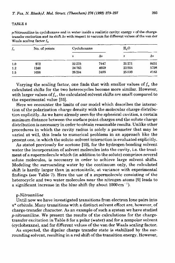
TABLE 8

p-Nitroaniline in cyclohexane and in water inside a realistic cavity: energy v of the eharge- transfer excitation and its shift Av with respect to vacuum for different values of the van der Waals scaling factor f,

No. of points Cyclohexane Hz0

V Av V Av

1.0 972 22 275 7447 21271 8451 1.2 1246 24 163 4959 23 924 5798 1.5 1698 26 234 3488 25 539 4183

Varying the scaling factor, one finds that with smaller values off, the calculated shifts for the two heterocycles become more similar. However, with larger values off, , the calculated solvent shifts are small compared to the experimental value [53].

Here we encounter the limits of our model which describes the interaction of the polarization charge density with the molecular charge distribution explicitly. As we have already seen for the spherical cavities, a certain minimum distance between the surface point charges and the solute charge distribution is necessary in order to obtain reasonable results. Unlike other procedures in which the cavity radius is solely a parameter that may be varied at will, this leads to numerical problems in an approach like the present one, in which the solute-solvent interaction is evaluated explicitly.

As stated previously for acetone [lo], for the hydrogen-bonding solvent water the incorporation of solvent molecules into the cavity, i.e. the treatment of a supermolecule which (in addition to the solute) comprises several solute molecules, is necessary in order to achieve large solvent shifts. Modeling the surrounding water by the continuum only, the calculated shift is hardly larger than in acetonitrile, at variance with experimental findings (see Table 7). Here the use of a supermolecule consisting of the heterocycle and two water molecules near the nitrogen atoms [9] leads to a significant increase in the blue shift (by about lOOOcm_“).

p-Nitroaniline Until now we have investigated transitions from electron lone pairs into

x* orbitals. Many transitions with a distinct solvent effect are, however, of charge-transfer character. As an example of such a system we have studied p-nitroaniline. We present the results of the calculations for the charge- transfer excitation in Table 8 for a polar (water) and for a nonpolar solvent (cyclohexane), and for different values of the van der Waals scaling factor.

As expected, the dipolar charge transfer state is stabilized by the surrounding solvent, resulting in a red shift of the transition energy. However,

294 T. Fox, N. RiischlJ. Mol. Struct. (Theo&em) 276 (1992) 279-297

it is most striking to note that the calculated solvent shifts are rather large, even for the unpolar solvent cyclohexane: 3488 cm-’ for f, = 1.5; nearly 7500cm-l for f, = 1.0. These results should be compared to those obtained from a spherical cavity model [9] where, for a radius estimated from the mass density, a red shift of 8OOOcm-’ with respect to the vacuum was calculated. In contrast to the findings in the previous section, the INDO calculation on nitroaniline gives better values for the dipole moment of both the ground state (8.7D (talc.) vs. 6.2D (exp.) [2]) and the charge- transfer state (19.6 vs. 16D) especially the calculated change of the dipole moment from ground to CT state which is in close agreement with the experimental value. These findings support the view that the unrealistic values of the solvent shifts are not due to the electronic structure method, but are caused by deficiencies in the cavity model. The shifts in the polar solvent water are hardly larger than in cyclohexane: for f, = 1.5 the difference amounts to 700 cm-‘; for f, = 1.0 to 1000 cm-‘. Compared to experimental observations [2] which yield a difference of about 3000 cm-l on going from cyclohexane to acetone, these values are far too small.

DISCUSSION

The examples given in this paper show that a straightforward application of the computational scheme presented to the calculation of solvatochromic shifts of absorption spectra may be quite successful in some cases, but rather problematic in others. Whereas the present cavity model yields a very satisfactory description of the ground state depression, no compar- ably reliable results are obtained for excitation energies. With a van der Waals scaling factor f, = 1.2, for acetone on the one hand, the relative shifts in different solvents can be well reproduced; for pyridazine and pyrimidine, on the other hand, they are too small. However, for p-nitroaniline with its pronounced change of the charge distribution during electronic excitation, the calculated shifts are far too large. These findings indicate that the physical model underlying a straightforward implementation of the cavity model is incomplete. This conclusion is quite similar to that obtained in a recent study of the n-x* solvent shift of acetone [lo].

Short-range interactions with directional characteristics have been modeled successfully by using a supermolecule which consists of the solute and a few solvent molecules at selected geometries [6-81.

One term usually omitted in modeling solvatochromic shifts is the dispersion interaction. Although arguments have been put forward for the contribution of dispersion forces to the ground state energies being of minor size in dipolar solvents [31], it has been shown that, even for polar molecules, the dispersion interactions are of the same order of magnitude as the long- range electrostatic contributions [54]. Therefore, it seems reasonable that

T. Fox, N. RGschlJ. Mol. Strut. (Theo&em) 276 (1992) 279-297 295

for accurate modeling of excitation energies (except for special cases) their influence cannot be neglected. Procedures for incorporating dispersion forces have been proposed [31]. Supplementaing the straightforward polarization model by this type of treatment (adapted to an arbitrary surface and extended to the calculation of excited states) should give a better description of solvatochromic shifts.

With the present results at hand, it seems that the success of models for calculating solvatochromic shifts which are based on a spherical cavity must be viewed with some caution. The success may even be fortuitous in some cases. The cavity radius (often not a well defined quantity) influences the results significantly, owing to the high powers that appear in the various multipole terms [17]. Its value may be adjusted to fit experimental data and, thus, may be used to compensate for the effects of the dispersion interaction, which are missing in these models. From this point of view, any cavity model for solvent effects which is restricted to pure electrostatic effects seems to be more consistent with a semi-empirical approach to quantum chemistry. At this level of sophistication an implementation of a cavity model with an ab initio formalism would seem inappropriate.

Besides these problems, the large solvatochromic shift calculated for nitroaniline may hint at some fundamental deficiency in the partitioning of the surface charge density into orientational and inductive parts. Its inade- quacy may become evident only if the charge distribution of the ground state and the excited state differ significantly. Further investigations with alternative partitioning schemes seem desirable [49].

With the present parametrization, the ZINDO/S model [29,30] often overestimates the polar character of the solute charge distribution as can be seen from a comparison of various calculated and experimental dipole moments. However, this deficiency should be compensated for by a slightly enlarged value of the scaling factor f,. Moreover, because this applies to all molecules investigated in a similar way, the deductions concerning a purely electrostatic model for the solvatochromic shifts should not be affected.

The difficulties found with the electrostatic cavity models which we have just discussed are of principle nature. Compared to them, we consider the representation of the solute charge distribution p(r) by Mulliken point charges in the calculation of the electrostatic potential of the solute to be a more technical approximation, which should have only minor consequen- ces for the conclusions reached in this paper.

CONCLUSIONS

We have presented a flexible yet efficient continuum model for the calculation of the electrostatic contribution to solvatochromic shifts. It is

296 T. Fox, N. RiischlJ. Mol. Struct. (Theochem) 276 (1992) 279-297

based on the INDO/S-CI electronic structure method and includes the interaction of the solute as determined self-consistently from the reaction field in a cavity of essentially arbitrary shape. The formalism is (in principle) able to account for solvent effects in the spectra of organic molecules. The trends in the spectra can be reproduced qualitatively; the quantitative agreement with observed solvatochromic shifts is sometimes unsatisfac- tory. We ascribe this to the inherent deficiency of current continuum methods that include only long-range electrostatic contributions of the solvent-solute interaction when modeling solvatochromic shifts. Direc- tional short-range interactions may be incorporated without effort using a supermolecule approach [9,10]. However, the modeling of the short range dispersion-type interactions presents a challenge for future work [31].

ACKNOWLEDGMENTS

We would like to thank M.C. Zerner, H.Heitele and J.-L. Rivail for valuable discussions. Th.F. is grateful for a Graduiertenstipendium of the TU Miinchen. This work has been supported by the German Bundesminis- terium fur Forschung und Technologie and by the Fonds der Chemischen Industrie.

REFERENCES

1 C. Reichhardt, Solvents and Solvent Effects in Organic Chemistry, 2nd edn., Verlag Chemie, Weinheim, 1988.

2 P. Suppan, J. Photochem. Photobiol. A, 50 (1990) 293. 3 0. Tapia, in R. Daudel, A. Pullman, L. Salem and A. Veillard (Eds.) Quantum Theory of

Chemical Reactions, Vol. II, Reidel , Dordrecht, 1981, p. 26. 4 J. Tomasi, Int. J. Quantum Chem, Quantum Biol. Symp., 18 (1991) 73-90. 5 A. Pullman, in R. Daudel, A. Pullman, L. Salem and A. Veillard (Eds.) Quantum Theory

of Chemical Reactions, Vol. II, Reidel, Dordrecht, 1981, p. 1. 6 J.T. Blair, J.D. Westbrook, R.M. Levy and K. Krogh-Jespersen, Chem. Phys. Lett., 154

(1989) 531. 7 D.C. Jain, D. de Gale and A.-M. Sapse, J. Comput. Chem., 8 (1989) 1031. 8 J. Koller and D. Ha&i, J. Mol. Struct., 247 (1991) 225. 9 M. Karelson and M.C. Zerner, J. Am. Chem. Sot., 112 (1990) 9405.

10 Th. Fox and N. RBsch, Chem. Phys. Lett., 191(1992) 33. 11 J.T. Blair, K. Krogh-Jespersen and R.M. Levy, J. Am. Chem. Sot., 111 (1989) 6948. 12 S.E. DeBolt and P.A. Kollman, J. Am. Chem. Sot., 112 (1990) 7515. 13 V. Luzhkov and A. Warshel, J. Am. Chem. Sot., 113 (1991) 4491. 14 G. Klopman, Chem. Phys. Lett., 1 (1967) 200. 15 H.A. Germer, Jr., Theor. Chim. Acta, 34 (1974) 145. 16 R. Constancieal and 0. Tapia, Theor. Chim. Acta, 48 (1978) 75. 17 J.G. Kirkwood, J. Chem. Phys., 2 (1934) 351. 18 L. Onsager, J. Am. Chem. Sot., 58 (1936) 1486. 19 J. Hylton, R.E. Christoffersen and G.G. Hall, Chem. Phys. Lett., 24 (1974) 501. 20 J.-L. Rivail and D. Rinaldi, Chem. Phys., 18 (1976) 233.

T. Fox, N. RBschlJ. Mol. Struct. (Theochem) 276 (1992) 27%297 297

21 22

23 24 25

26 27 28 29 30 31 32 33 34

35 36 37 38 39 40 41 42 43 44

45 46

47 48 49 50 51 52

53 54

S. Miertui;, E. Scrocco and J. Tomasi, Chem. Phys., 55 (1981) 117. K.V. Mikkelsen, H. Agren, H.J.Aa. Jensen and T. Helgaker, J. Chem. Phys., 89 (1988) 3086. D. Rinaldi, M.F. Ruiz-Lopez and J.-L. Rivail, J. Chem. Phys., 78 (1983) 834. K.V. Mikkelsen, E. Dalgaard and P. Swanstrem, J. Phys. Chem., 91 (1987) 3081. C. Aleman, F. Maseras, A. Lledos, M. Duran and J. Bertrbn, J. Phys. Org. Chem., 2 (1989) 611. M.F. Ruiz-Lopez, D. Rinaldi and J.-L. Rivail, Chem. Phys., 110 (1986) 403. J. Applequist, J. Phys. Chem., 95 (1991) 3539. M.A. Thompson and M.C. Zerner, J. Am. Chem. Sot., 113 (1991) 8210. J.E. Ridley and M.C. Zerner, Theor. Chim. Acta, 32 (1973) 111. J.E. Ridley and M.C. Zerner, Theor. Chim. Acta, 42 (1976) 223. D. Rinaldi, B.J. Costa-Cabral and J.-L. Rivail, Chem. Phys. Lett., 125 (1986) 495. F. Floris and J. Tomasi, J. Comput. Chem., 10 (1989) 616. E.G. McRae, J. Phys. Chem., 61 (1957) 562. J. Hyltonn, McCreery, R.E. Christoffersen and G.G. Hall, J. Am. Chem. Sot., 98 (1976) 7191. B. Linder, Adv. Phys. Chem., 12 (1967) 225. M.L. Connolly, Quantum Chem. Prog. Exch. Bull., 1 (1981) 75. R.J. Zauhar and R.S. Morgan, J. Comput. Chem., 9 (1988) 171. J. Warwicker and H.C. Watson, J. Mol. Biol., 157 (1982) 671. M.K. Gilson, K.A. Sharp and B.H. Honig, J. Comput. Chem., 9 (1988) 327. R.J. Zauhar and R.S. Morgan, J. Comput. Chem., 11 (1990) 603. Th. Fox, N. Rosch and R.J. Zauhar, J. Comput. Chem., in press. H. Agren, CM. Llanos and K.V. Mikkelsen, Chem. Phys., 115 (1987) 43. R. Cimiraglia, S. Miertuj: and Tomasi, Chem. Phys. Lett., 80 (1981) 286. R. Bonaccorsi, C. Ghio and J. Tomasi, in R. Carbo (Ed.), Current Aspects of Quantum Chemistry 1981, Studies in Physical and Theoretical Chemistry, Vol. 21, Elsevier, Amsterdam, 1982, p. 407. W. Heiden, M. Schlenkrich and J. Brickmann, J. Comput. Aided Mol. Des., 4 (1990) 255. R.J. Woods, M. Khalil, W. Pell, S.H. Moffat and V.H. Smith, Jr., J. Comput. Chem., 11 (1990) 297. C. Giessner-Prettre and A. Pullman, Theor. Chim. Acta, 25 (1972) 83. R. Bonaccorsi, R. Cimiraglia and J. Tomasi, J. Comput. Chem., 4 (1983) 567. J.E. Brady and P.W. Carr, J. Phys. Chem., 89 (1985) 5759. W. Liptay, Z. Naturforsch. Teil A, 20 (1965) 1441. A.T. Amos and B.L. Burrows, Adv. Quantum Chem., 7 (1973) 289. R.C. Weast (Ed), Handbook of Chemistry and Physics, 69th edn. CRC Press, Boca Raton, FL, 1988. H. Baba, L. Goodman and P.C. Valenti, J. Am. Chem. Sot., 88 (1966) 5410. E.S. Marcos, M.J. Capitln, M. Galln and R.R. Pappalardo, J. Mol. Struct. (Theochem), 210 (1990) 441.

Documents

On the cavity model for solvent shifts of excited states — a critical appraisal