ON THE CAPTURE-RECAPTURE METHODS OF ESTIMATING POPULATION

SIZE

BYNYANGOMA^STEPHEN ODUNDO

DEPARTMENT OF MATHEMATICS UNIVERSITY OF NAIROBI

This dissertation is submitted in partial fulfillment of the degree of Master of Science in Mathematics in the University of Nairobi.

UNIVERSITY OF NAIROBI. JULY, 1991.

-11-

DECLARATION

This dissertation is my original work and has not been presented for a degree in any University.

SignatureNYANGOMA STEPHEN ODUNDO.

This dissertation has been submitted for examination with my approval as a University Supervisor.

V)-lii-

ACKNOWLEDGEMENTThis dissertation would not have been written without

the assistance of many.First and foremost, I am grateful to my sponsor the

University of Nairobi for granting me a Scholarship that enabled me to pursue the postgraduate course.

I would like to express my sincere thanks to my supervisor Prof. J. W. Odhiambo, without whose guidance and close supervision, I may not have completed this work. Prof. Odhiambo has been of utmost assistance in all the stages of preparation of this dissertation and indeed the whole course. I am also grateful to my lecturers Dr. Manene and Prof. Ottieno, whose lectures in variousfields provided me with background knowledge and inspiration to embark on this study. I am also very grateful to Prof. G. F. Seber for his advise and assistance during the preparation of this dissertation.

I owe the former Director of the Kenya Marine and Fisheries Research Institute (K. M. F. R. I.), Mr. Alela a word of thanks for releasing me to pursue the postgraduate course. I am also grateful to my colleague at theK.M.F.R.I., Mr. Ogunja for all the assistance he offered me at the end of the course. I wish to express my sincere gratitude to my colleagues in the course Mr. Bodo and Miss. Matu, who have been a source of great encouragement and company during the entire course.

I hereby wish to express deep appreciation to my parents Mr. and Mrs. Nyang'oma for their active supportand encouragement during the entire education. Finally, I want to say thank you to all those whose names do notappear here but who in one way or the another helped me attain my goal.

-VI-

CONTENTS.

Title.Declaration.Acnowledgement.Contents.Sumary of Contents.

PAGEi

iiiiiivv

CHAPTER ONE: Basic Principles Underlying the Capture-recapture Methods. 1

1.1 The Capture-recapture Method. 11.2 Notation and Terminology. 61.3 Some Statistical Methods Used in

Capture-recapture studies. 10

CHAPTER TWO: Literature Review and Statement of theProblem. 26

2.1 Literature Review. 262.2 Statement of the Problem. 83

CHAPTER THREE : Single-Mark Release. 853.1 Estimation. 853.2 Validity of the Assumptions. 973.3 Estimation from Several Samples. 1353.4 Inverse Sampling Methods. 1403.5 Comparing^Two Populations. 1493.6 Estimation by Least Squares. 152

CHAPTER FOUR: Multiple Marking. 1564.1 Schnabel Census. 1564.2 Inverse Multiple Sample Census. 2154.3 The Multi-Sample Single Recapture Census. 2174.4 Conclusions. 224

APPENDIX. 228REFERENCES. 238

- v-

SUMMARY OF CONTENTS.This dissertation is an attempt to study the

capture-recapture models estimation of closed population size. Where possible, the assumptions underlying various models have been discussed in some detail. Departures from various assumptions have also been discussed.

Chapter one, outlines the basic principles underlying the capture-recapture method of estimating population size. Some statistical methods used capture-recapture studies are also presented.

In Chapter Two, a very extensive literature review of the most work done on both open and closed populations is presented. A statement of the problem is also outlined in this Chapter.

In Chapter Three, we discuss various models based on Single-Mark release experimental set-up. The various assumptions underlying these models have also been discussed in some detail. The properties of the Petersen estimate have also been discussed. Inverse sapling scheme and the models based on it are also discussed.

In Chapter four, we discuss the models based on the Schnabel sapling scheme. Properties of the estimates derived from these models have also been discussed. Some Regression models have been presented. The testing of the underlying assumptions have been presented. We also discuss the models based on constant probability of capture. Inverse Multiple sampling census together with the models based on it have also been discussed. The models based on the Multi-Single recapture census have also been presented. Conclusions are in section 4.4 .

Lastly we give an appendix and references.

1

CHAPTER ONE

BASIC PRINCIPLES UNDERLYING THE CAPTURE-RECAPTURE METHOD

1.1 THE CAPTURE-RECAPTURE METHOD

The estimation of the total population size

of animal populations is of great importance in

a variety of biological problems. These problems

may relate to population growth, ecological

adaptation, genetic constitution, natural selection

and evolution and so on. Obvious practical

consequences are the maintenance of human food

supplies and control of insect pests. For human

comiTiun I ties, procedures employing fixed sampling

units are available, but for mobile populations,

other methods must be used. Techniques for estimating

total population size of organisms which are mobile

and wary of man are still in relatively primitive

stage of development and while indices of abundance

may be available in a variety of forms, the assessment

of total size with any degree of precision generally

requires considerable ingenuity and effort. Thus the

number of fish of a given species present in a lake

is not an easily accessible parameter. By a judicious selection of times and places to set nets each year,

however, the fishery biologist may be able to monitor

change in relative abundance with little difficulty.

2

Among the techniques which have been developed for

estimating the total population size, the capture-recapture

method is the most widely used. In its simplest and most

commonly applied form, the capture-recapture experiment

is a two sample experiment in which the members of the

first sample are marked in some recognizable manner and

returned to the population. The proportion of marked

individuals appearing in the second sample is then

regarded as an estimate of the proportion marked in the

population. Since the number of marked individuals in

the population is known, this reasoning leads directly

to an estimate of the total population size. Thus if n^

individuals are marked and released in the first sample

and m2 marked individuals are subsequently recaptured

in a sample of size n2, then the population size is

estimated by N = n^ n2/m2 on the assumption that

m2/n2 estimates n- /N.

In more extensive investigations the sampling

and marking continues intermitently over a period of time,

the unmarked individuals captured on each occasion being

marked before being returned with the others to the

population. Distinct "batch marks" are sometimes used

in such studies; that is on each sampling occasion all unmarked individuals are given an identical batch-mark

but recognizably different mark is used for each

successive batch. More commonly in the multiple sample

experiment the "mark" consists of a numbered tag which is

attached to the individual and thereafter uniquely

identifies it. In some multiple sample experiment?,

3

both the marked and unmarked individuals are

distinctively marked any time they are caught

and then released to the population. Each time an

individual is captured, a record is marked for it or

on it to show the recapture history. We shall here

consider statistical aspects of k-sample capture-

recapture experiment.

The k-sample capture-recapture experiment

Sample size on any one occasion is usually

limited by the amount of capture gear and manpower

which can be brought into operation at any one time.

Under such economic restrictions the only feasible

means of increasing the precision of the experiment

may be steadily increased by marking all unmarked

individuals captured on each sampling occasion and

returning the entire sample to the population.

The general field experiment is similar for all

capture-recapture studies. At the beginning of the

study, a sample of size n- is taken from the

population. On each occasion the catch is considered

as a random sample of individuals from the population.

That is each individual in the population has an equal

chance of being captured on any given occasion. Each

time an individual is caught a record is marked for it

or on it to show the occasion of capture. The

individual is then returned into the population.

After allowing time for the marked and unmarked animals

to mix, a second sample of size n2 is taken. The

second sample normally contains both marked and unmarked

animals. In some methods the unmarked animals are

marked and all captured animals are released back into

the population, where as some methods demand that, both

the marked and unmarked be marked distinctively and then

released into the population. This procedure proceeds

for k periods where k >_ 2.

During the course of this sampling experiment the

population itself may undergo changes through such

processes as mortality, emigration and immigration;

and conceivably, the risks associated with these processes

may vary with the previous capture history of an

individual. In particular, the untagged portion of the

population may be subject to different rates of mortality,

emigration and immigration from the tagged portion.

The early models assumed deterministic changes, constant

over different periods, where as the later models

(stochastic) considers variable changes. Since stochastic

models describing capture-recapture studies have recently

been shown not only to be less complicated to analyse

than their corresponding deterministic models but also

to provide more valid results, these methods should

totally supersede their deterministic counterperts.

However, if it is assumed that no changes occur over the

sampling period, then the population is considered

closed.

- 1] -

5

ASSUMPTIONS:

Before any mathematical formulation of capture-

recapture models can be done, there are certain basic

assumptions that have to be made about the population

under study. These assumptions vary from one model

to the other. We now give some of the assumptions which

are made for most of the capture-recapture models;

these are:

(i) animals do not loose their marks;

(ii) sampled animals are classified correctly as

marked and unmarked according to when they

were recaptured;

(iii) sampling is random with respect to mark status

so that, either

(a) every animal has the same chance of

recapture, or

(b) if there exist strata within the population

such that, by size, behaviour or any other

variation, different strata have different

chances of recapture, then the marked

animals belong to these strata in exactly the same proportions as the occurrence of the strata in the whole population.

The following assumption holds for strictly

closed population models.

(iv) either (a) the population is really closed, or

6

(b) there is neither recruitment nor immigration

(both of which affect unmarked animals only),

and death and emigration affect marked and

unmarked animals equally, or

(c) knowledge is available from other sources

which permit an allowance to be made for

migration, birth, and death prior to the

analysis of the data.

We shall give more assumptions later as we study each model.

NOTATION AND TERMINOLOGY;

NOTATION

In this desertation we shall adopt the international

notations used by F.A.O. for fishery research and

especially the " mnemonic " notation. For example, N

and n denote the number of individuals in the population and sample respectively; M and m refer to the number

of marked (or tagged members) of the population and

sample respectively s represents the number of samples

and so on. Each chapter will be self contained as

far as the notation is concerned.

Some statistical symbols are required: E[y], o[y]

v[y] (= a [y], c[y] (= a[y]/E[y]) will represent the

mean, standard deviation, variance and coefficient of

variation respectively, of the random variable y, where as cov[x,y] will denote the covariance of the

random variables x and y, and E[x|y], v[x|y]

7

are the mean and variance of x conditional on fixed

y. The symbols z a and tk [a] will represent the

100a percent upper tail for the values of standard

normal distribution and the t-distribution with

k-degreeo of freedom, respectively.

Occasionally the symbols 0[N] and o[N] will

be used; if g is a function of N, then g(N) = 0[N]

if there exists an integer N-j and a positive number

A such that, for N> f^, cd(|sCN)/N | < A; g(N) = oi_N]

if lim {g(N)/N} = 0. Roughly speaking, 0[n 1

means "of the same order of magnitude as N when N is

large", while o[N] means "of smaller order of

magnitude than N when N is large".

If x has a multivariate normal distribution

with mean vector £ and variance covariance (dispersion)

matrix E , we shall write x ^ N(_0,Z).

All logarithms written logx will be to base

e unless otherwise.

TERMINOLOGY

The size of an animal population in a given area

will be determined by the process of immigration

(or movement into an area), emigration (or movement

out of the area), total mortality, and recruitment.

Total mortality: In dealing with exploited populations,

we shall usually subdivide total mortality into mortality

due to exploitation and natural mortality, i.e. mortality due

8

to natural processes such as predation, disease,

clLmatLcconditions: Contrary to some authors,

emigration is not included here under "mortality".

We shall also distinguish between mortality rate

and Instantenous mortality rate as follows:

Let (p be the probability that an animal survives tfor the period of time [0,t], then if Nq animals are

alive at time zero we would expect = NQ<f>t to be

alive at time t.

The proport Lon (pt , sometimes expressed as a percentage,

is called the survival rate over period t, and

1 - <j> is called the mortality rate over period t.

If, however, the mortality rate may be regarded as a

Poisson process with parameter y , that is the

probability that an individual dies In the time

interval (t, t+St) is y6t + o(6t), then

. -pt'f’t = e

dN~dt~ = liNt 5

and the parameter \i is called the instantanous

mortality rate.

Mean L1 fe_Exnej^ taacy^i L e t Y be t h e t lm e a t whlch

a member of N dies.o

Then ,

F[y] = Pr[Y < y]

= 1 - Pr[Y > y]= 1 - Pr[animal survives until time y

9

= 1 - exp(-py)

and Y has the probability density function

f(y) =F'(y) = ue“uy , (y > 0).

Therefore the mean life expectancy is00

E[Y] = / pye"My dy .o

= 1/n

= - 1/log <$>1 .

Recruitment: By recruitment, we shall refer to those

animals born into the population or, where applicable,

those animals which grow into the catch.able part of the population. In fishery research, recruitment some times

denote those fish which grow into the class of legally

catchable fish. Thus we do not treat immigration as a

component of recruitment.

Open and closed populations: A population which

remains unchanged during the period of investigation

(i.e. the effects of migration, mortality and recruitment

are negligible) is called a closed population. If a

population is changing due to one or more of the above

processes operating, then the population is said to be open.

- 10 -

1#3 SOME STATISTICAL METHODS USED IN CAPTURE-RECAPTURE

STUDIES:

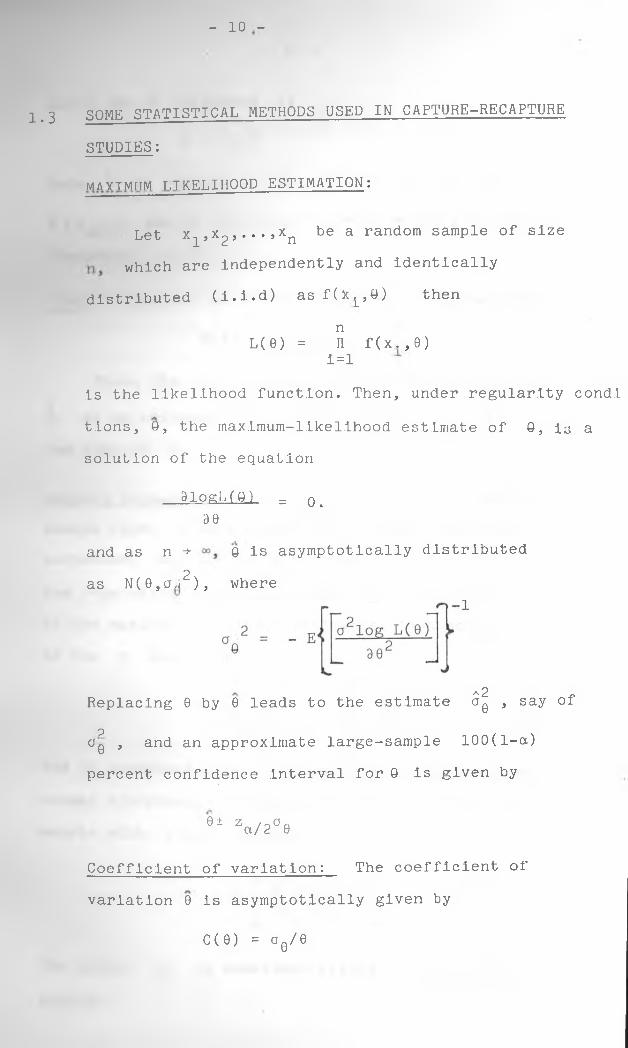
maytmiim T.TKELIHOOD ESTIMATION:

is the likelihood function. Then, under regularity condi

t.Lons, 0, the maximum-likelihood estimate of 0, is a

solution of the equation

_91ogL_(0_L = o.90

and as n + 0 is asymptotically distributed2as N(0,0 w ), where

Let x1,x2,--.,xn be a random sample of size

which are Independently and identically

distributed (i.i.d) as fCx^O) then

nL( 0) = n f(x.}0)

i=l

2Replacing 0 by 0 leads to the estimate o0 , say ofp

Oq , and an approximate large-sample 100(1-a)

percent confidence interval for 0 is given by

0± z /o0 Q a /2 0

Coefficient of variation: The coefficient of

variation 0 is asymptotically given by

C(0) = oQ/0

11

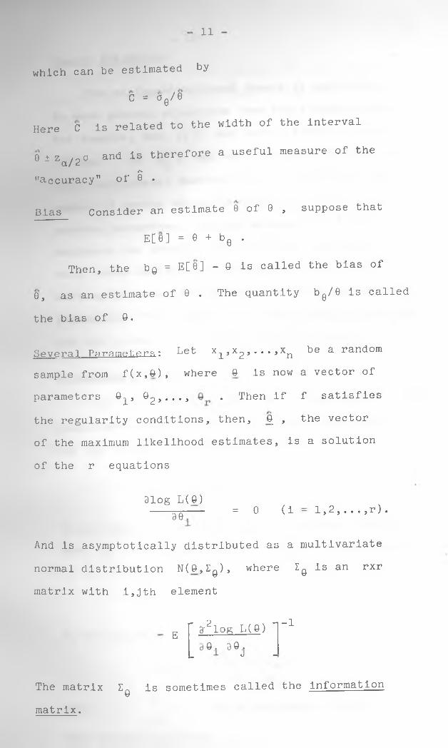
which can be estimated by

C = O q /9

Here C Is related to the width of the interval

B + z , a and is therefore a useful measure of the " a/2 A"accuracy" of 0 .

Bias Consider an estimate 0 of 0 , suppose that

E[0] = 0 + b0 .

Then, the bQ = E[0] - 0 is called the bias of

0, as an estimate of 0 . The quantity b0/0 is called

the bias of 0.

Several Parameters: Let x1)x2 J*,,Jxn be a randomsample from f(x,0), where Q is now a vector of

parameters 0^, 02,..., • Then if f satisfies

the regularity conditions, then, Q_ , the vector

of the maximum likelihood estimates, is a solution

of the r equations

31og L(0)--- g-Q--- = 0 (i - 1,2 , . . . , r ) .

And is asymptotically distributed as a multivariate

normal distribution N(0,Iq ), where Zq is an rxr

matrix with i,jth element

E f ar2log L( 6 ) l " 1d 0 . 0 0. J —

The matrix Zg is sometimes called the Information

matrix.

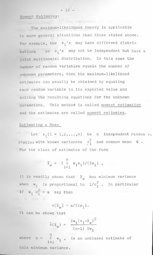
12Moment Estimates:

The maximum-likelihood theory is applicable

to more general situations than those stated above.

For example, the x ^ s may have different distri­

butions or x i ' s may not be independent but have a joint multinomial distribution. In this case the

number of random variables equals the number of

unknown parameters, then the maximum-likelihood

estimates can usually be obtained by equating

each random variable to its expected value and

solving the resulting equations for the unknown

parameters. This method is called moment estimation

and the estimates are called moment estimates.

Estimating a Mean

Let x.(i = l,2,...,n) be n independent random va2riables with known variances ck and common mean 0 .

For the class of estimates of the form

xw = (Lfx wix1)/(Ewi) •

it is readily shown that x has minimum variancew2when w^ is proportional to 1/ck . In particular

2if w^ (K = a say then

v[xw ] = a/( Zw.L) .It can be shown that

v (x ) = w '^ l (xl-xw ) (n-1) Zw.

where n =n w

i=i ;is an unbiased estimate of

this minimum variance.

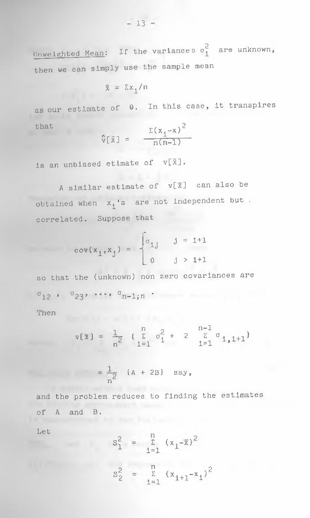
13

Unweighted Mean: If the variances c2 are unknown

then we can simply use the sample mean

X = Lx ± /n

as our estimate of 0 . In this case, it transpires

thatv[x] =

Z(xi-X)2nTn-l)

is an unbiased etimate of v[x] .

A similar estimate of

i—iIX1_1> can also be

obtained when xi ’s are not independent but .

correlated. Suppose that

cov(x1,xj. ) = -

•<“D•H* & J = i+1

_ 0 J > i+1

so that the (unknown) non zero covariances are

°12 5 U 2 3 ’ °n-l;n *

Then

n p n-1v[x] = ^ { Z o. + 2 Z o }

n2 i=l 1 i=l ’

= KrtA + 2B} say, n

and the problem reduces to finding the estimates

of A and B.

LetZ (x,-x)

i=l 1

S22nZ

i=l(xi+1-xi

2

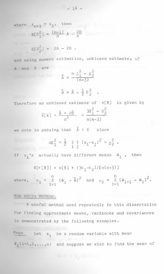
where xn+i " xi> then

E[s2] = n 1 ■*- A - — iJ n n

E[S*] = 2A - 2B .

and using moment estimation, unbiased estimates of

A and B are2 2

n S 1 " S 2A = T n ^ U

a- i pB = A - S 2

Therefore an unbiased estimate of v[x] is given by

v[x] = A + 2B 3^1 S2n n(n-3)

we note in passing that A > 0 since

_ 2 _ 1 v v , v n2 2nS — 2 2 E ( x —x ) > S 2 *i j

If x^'s actually have different means 0^ , then

E[v [x] ] = v[x] + (3c1-c2)/[n(n-3) ]

nwhere, c-, = E (0. - 0) and cp = E (9.

i=! 1

nZ

1=1

THE DELTA METHOD:

A useful method used repeatedly in this dissertation

for finding approximate means, variances and covariances is demonstrated by the following examples.

Mean Let x^ be a random variable with mean

el(i=l,2,...,n) and suppose we wish to find the mean of

15

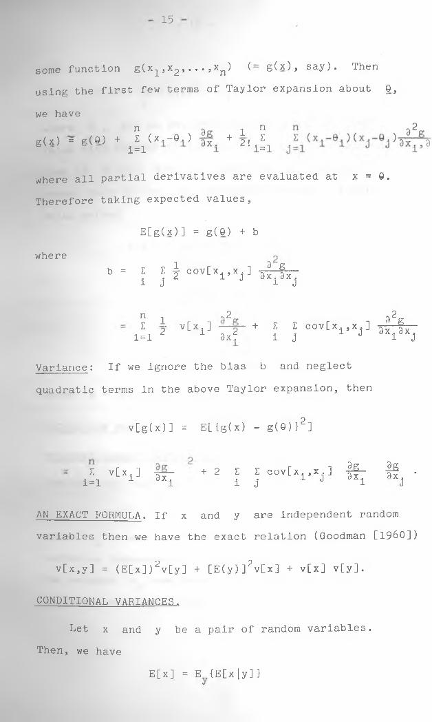
some function g(x^)X2 j•••jx^) ( 6(x) j say). Then

using the first few terms of Taylor expansion about 0,

we have

g(x) = g(Q) +nZ (x.-0.)

i=l+ 1

2 !nZ

i=l

where all partial derivatives are evaluated at x = 0.

Therefore taking expected values ,

whereb =

E[g(x)] = g(9) + b

Z Z ^ c o v [x . , x . ] 9 f ■ ■■i j 2 1 J 3xi3xj

n n ~ 2 ^2I o- v[x. ] + Z Z cov[x,,x.] a ■fy—

1=1 2 1 3xf i j 1 J dxidxj

Variance: If we ignore the bias b and neglect

quadratic terms in the above Taylor expansion, then

v[g(x)] a E[{g(x) - g(e)}2]

+ 2 Z Z cov[x,,x,] -If- If • i j 1 J °Xi Xj

Z v[x.] ^i=l 1 9xi

AN EXACT FORMULA. If x and y are independent random

variables then we have the exact relation (Goodman [I960])

v[x,y] = (E[x])2v[y] + [E(y)]2v[x] + v[x] v[y].

CONDITIONAL VARIANCES.

Let x and y be a pair of random variables.

E[x] = E (E[x |y] }V

Then, we have

- 16 -

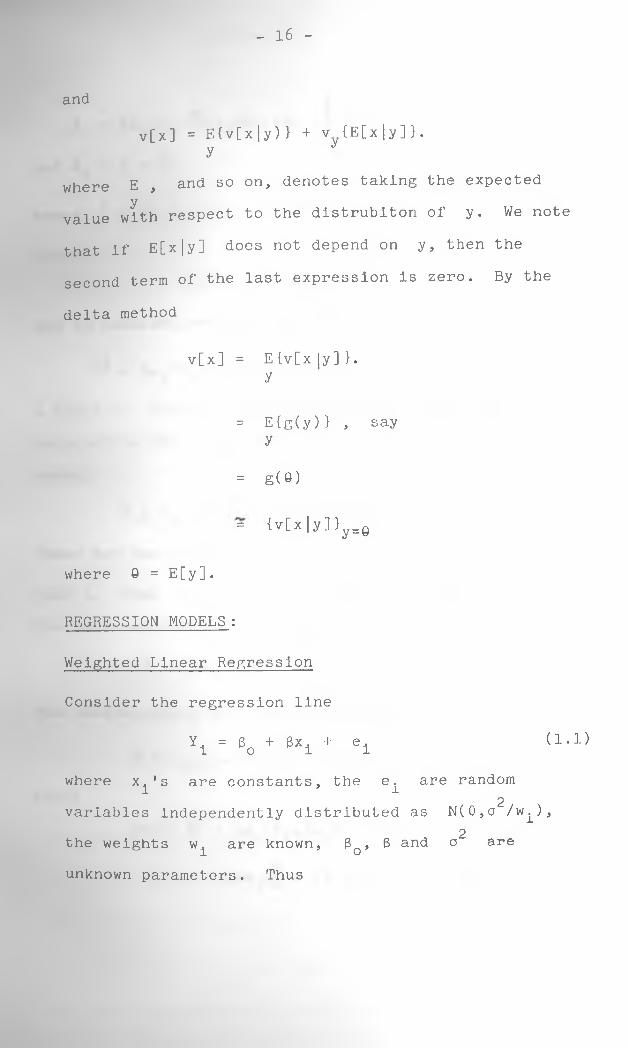
and

v[x] = E{v[x|y)} + v {E[x|y]}.y *

where E , and so on, denotes taking the expected y

value with respect to the distrubiton of y. We note

that if E[x|y] does not depend on y, then the

second term of the last expression is zero. By the

delta method

v[x] = E {v[x |y] }.y

= E {g(y)} , sayy

= g(o)

= <v[x|y]}y=0

where 0 = E[y].

REGRESSION MODELS : * 2

Weighted Linear Regression

Consider the regression line

Y x = 60 + 8x1 + e± (1.1)

where x^fs are constants, the e^ are random2variables independently distributed as N(0,o /w^),

2the weights w^ are known, 3oJ 3 and o are

unknown parameters. Thus

17

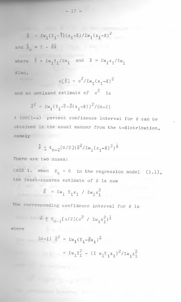
3 = Z w ^ Y ±-Y)(x1-x)/Zwi(xl-x)2

and 3 = Y - 3xo

where Y = Zw^Y^/Zw^ and x = Zw^x^/Zw^

Also,v[3] = a2/Zwi(xi-x)2

2and an unbiased estimate of a Is

a2 = Zw1(Yi-Y-3(xi-x))2/(n-2)

A lOO(l-a) percent confidence interval for 3 can be

obtained in the usual manner from the t-distribution, namely

3 + tn_2[a/2](c2/Zwi(xi-x)2)2

There are two cases:

CASE 1. When 3Q = 0 in the regression model (1.1),

the least-squares estimate of 3 is now

3 = Zw^ Y^x^ / Zw^x2

The corresponding confidence interval for 3 is

3 t tn_it°/2](o2 / Zw^x2)2

(n-l) a2 = j:wi(Yi-3x1)2

= 2wiYi “ ^ w xy 1x 1)2/^w 1x 2

where

18 -

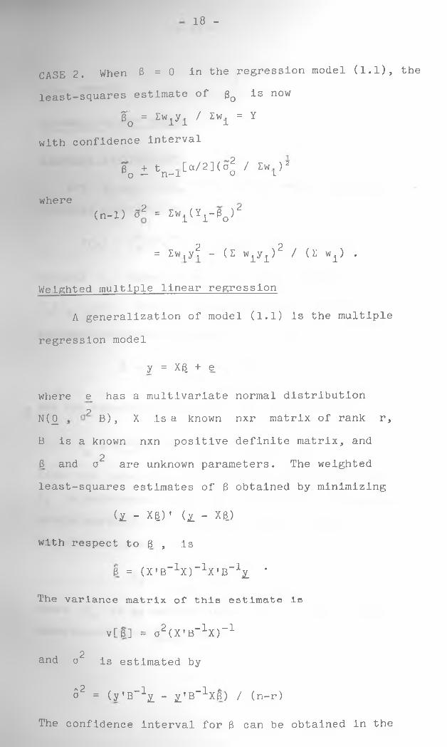
CASE 2. When 3 = 0 In the regression model (1.1), the

least-squares estimate of 0Q is now

§o = £wiyi / Zw± = Y

with confidence interval

B + tn [a/2](o2 / Zw )2 o — n-i o ±

where(n-X) a2 = Iw1(Y1-6o )‘i

= XwLy? - (£ w ^ ) 2 / (X w^) .

Weighted multiple linear regression

A generalization of model (1.1) is the multiple

regression model

y = XB_ + e

where e_ has a multivariate normal distributionpN(£ b ), X is a known nxr matrix of rank r,

B is a known nxn positive definite matrix, and 23 and a are unknown parameters. The weighted

least-squares estimates of 3 obtained by minimizing

( i - x &)1 (£ - xe j

with respect to 6 , Is

3 = (X,B"1X)”1X ,B_1^ *

The variance matrix of this estimate lo

v[3] = a2(X'B"1X)"12and o is estimated by

52 = (y'B-1x - £'B-1xe) / (n-r)

The confidence interval for 3 can be obtained in the

19

usual manner.

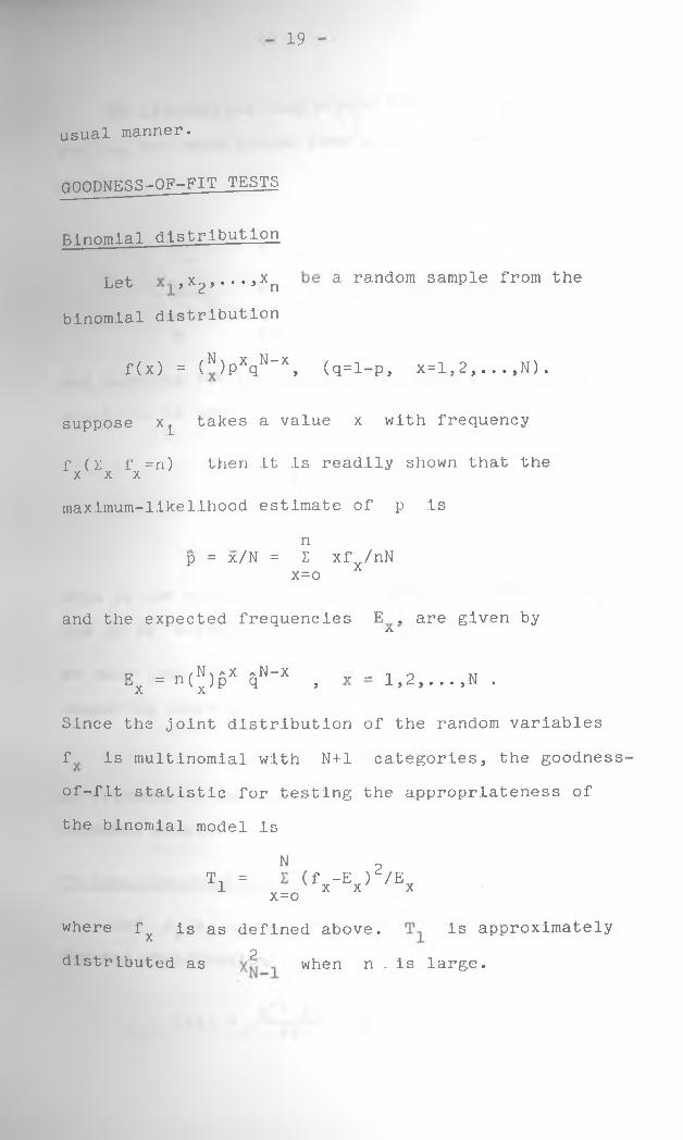
GOODNESS-OF-FIT t es ts

Binomial distribution

Let , * 2 5 * * ' 9 xn a ran^om samPle from thebinomial distribution

f(x) = (“ )pxqN_X, (q=l-p, x=l,2,...,N).

suppose x L takes a value x with frequency

f (y. f =n) then it is readily shown that the x x xmaximum-likelihood estimate of p is

np = x/N = E xf /nN

x=o X

and the expected frequencies E . are given byA

„ _ „/NxaX aN-X „ _ 0 MEx — a ( x) p Q f 1j 2,. . . ,N .

Since the joint distribution of the random variables

f is multinomial with N+l categories^ the goodness-

of-f.Lt statistic for testing the appropriateness of

the binomial model is

T1 = " (fx-Ex )2/Exx=owhere f y is as defined above. is approximately

Pdistributed as when n , is large.

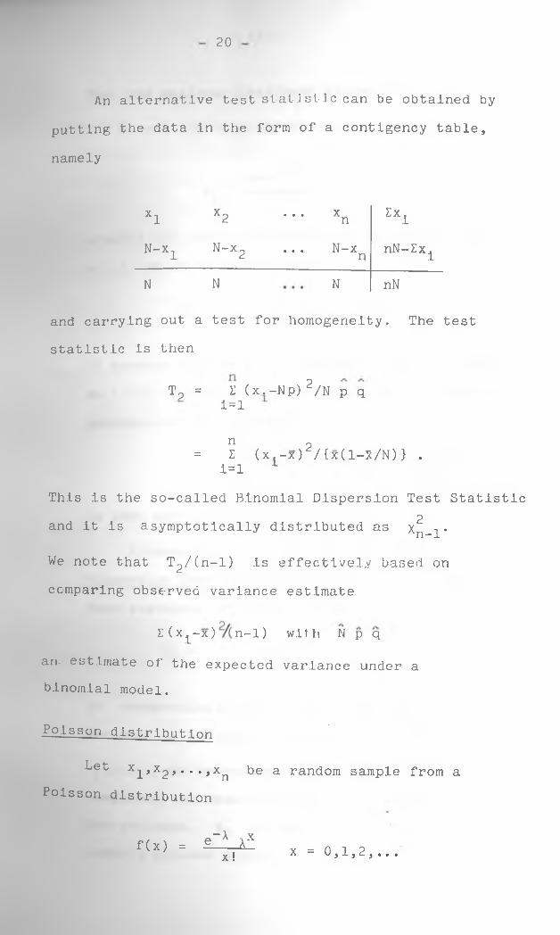
20

An alternative test sl at j stlc can be obtained by

putting the data in the form of a contigency table,

namely

X1 X2 ... Xn Exi

N-x1 N-x 2 . . . N-xn nN-Ex^

N N N nN

and carrying out a test for homogeneity. The test

statistic is then

Tp = E (x.-Np)^/N p q i=l

n 2= Z (x.-x) /{x(l-X/N)} .

i = l 1

This is the so-called Binomial Dispersion Test Statistic2and it is asymptotically distributed as Xn-1*

We note that Tp/(n-l) is effectively based on

comparing observed variance estimate

E (x^-x) n-1) with N p q

an. estimate of the expected variance under a binomial model.

Poisson distribution

Let x^,x2,...axn be a random sample from a Poisson distribution

f(x) = £ ± Xxx! x = 0,1,2, ...

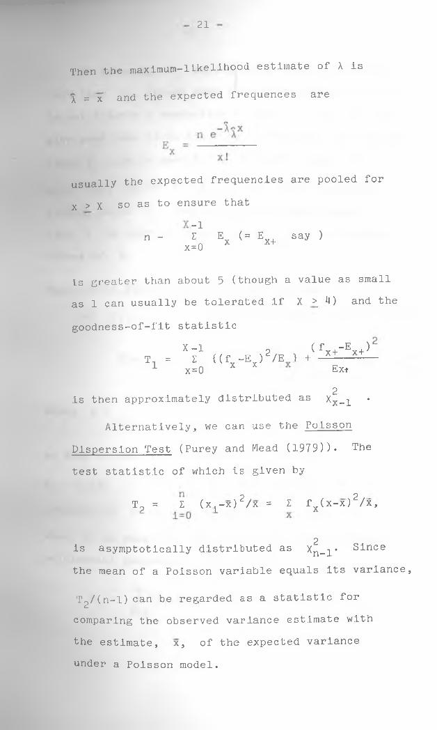
21

Then the maximum-likelihood estimate of A is

X = x and the expected frequences are

usually the expected frequencies are pooled for

x > X so as to ensure that

n " ^ Ex (= Ex+ say }x=0

is cheater than about 5 (though a value as small

as 1 can usually be tolerated if X >. 4) and the

goodness-of-fit statistic

X -1 2 (fx+-Ex+ )T. = I {(f - E / / E ) + X 1 x=0 x Ext

is then approximately distributed as 2Xx-1 •

Alternatively, we can use the Poisson

Dispersion Test (Purey and Mead (1979))* The

test statistic of which is given by

Tp = Z (x l-x )2/x = Z fx(x-x)2/x,

2is asymptotically distributed as Xn_^* Since

the mean of a Poisson variable equals its variance,

Tp/(n-l) can be regarded as a statistic for

comparing the observed variance estimate with

the estimate, x, of the expected variance

under a Poisson model.

22

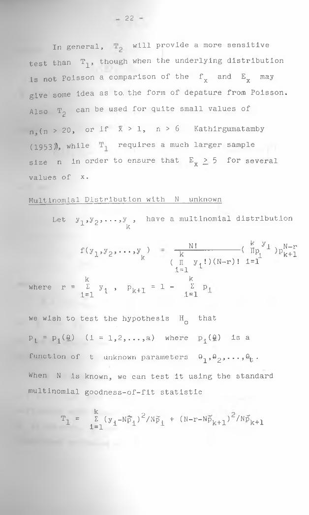
In general, will provide a more sensitive

test than 1^, though when the underlying distribution

Ls not Poisson a comparison of the fx and Ex may

give some idea as to. the form of depature from Poisson.

Also T2 can be used for quite small values of

n (n > 20, or if x > 1, n > 6 Kathirgumatamby

(1953))j while requires a much larger sample

size n in order to ensure that Ex _> 5 for several

values of x.

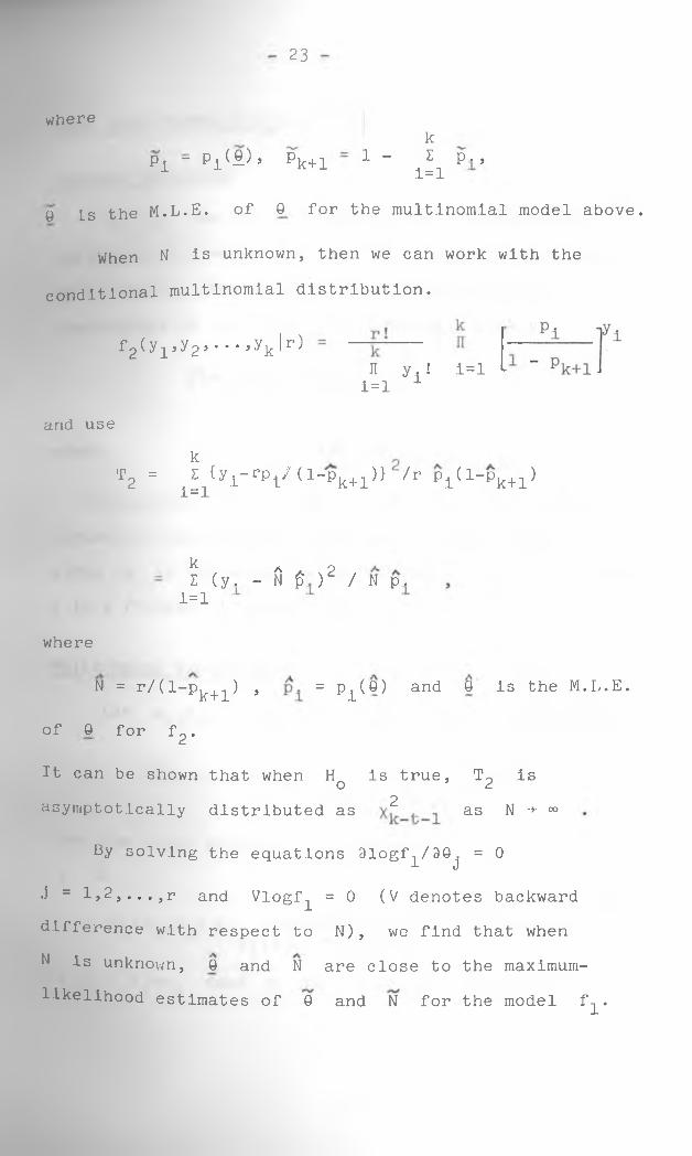
Multinomial Distribution with N unknown

Let y,,y9,...,y , have a multinomial distribution 1 d k

f (y-, 3yp3.. • 5y )1 kN!

k

kwhere r = Z y , p

.1=1 1 k+1

( n y1!)(N-r)! i=l i=l L

k= 1 - 2 P 1

1=1

, * yi s N-r npi pk+l

we wish to test the hypothesis Hq that

P L = P L(0) (i = 1,2,...,a) where p^CO) is a

function of t unknown parameters 9^, ©2 , . . . , 0, .

When N is known, we can test it using the standard

multinomial goodness-of-fit statistic

T., =kZ

i=l(y1-Np1)2/Np1 + (N-r-Npk+1) /Npk+1

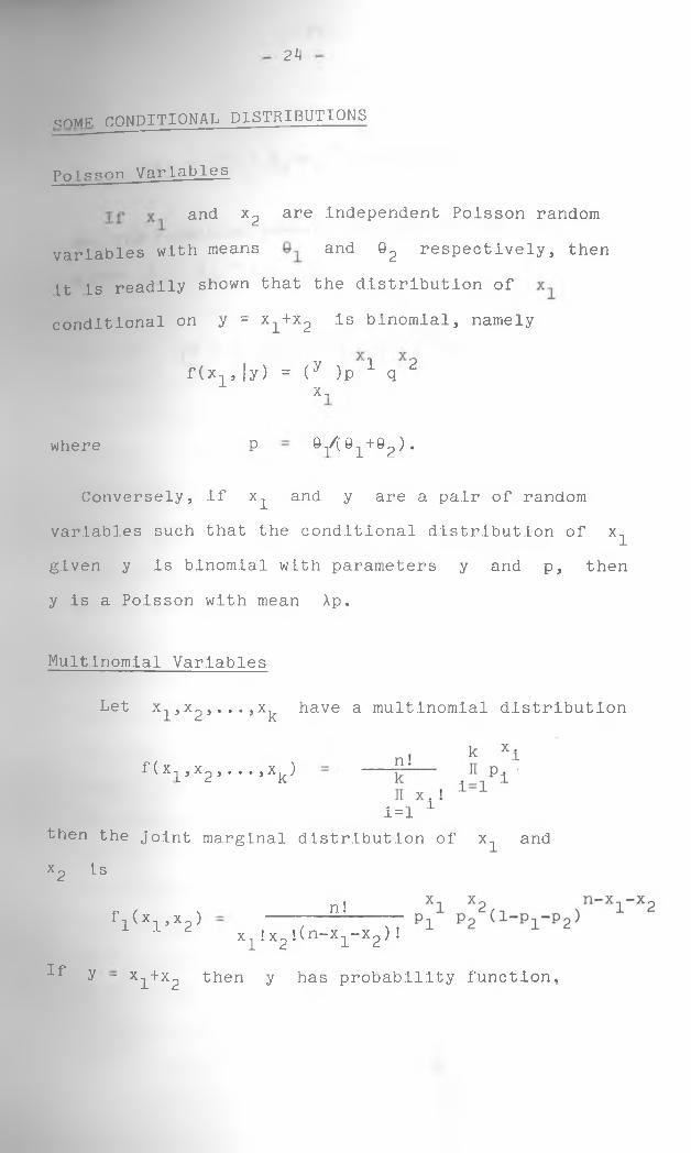
23

where

Pi - Pj/i) > pk+lk

1 - I p .,1=1

G Ls the M.L.E. of 9 for the multinomial model above.

When N is unknown, then we can work with the

conditional multinomial distribution.

f2^yi>y2 f •* * *^k r^n y,! i=l Li = l x

and usek

T2 = if1{yi-rPl/ (l-Pk+1)} /r pi(1-pk+l)

k ft A x2Z (y. - N p ) / N p.i=l

where

N = r/(l-p^.+^) , = p^(6) and G is the M.L.E.

of 0 for f2.

It can be shown that when H is true, T0 iso d2asymptotically distributed as as N -*■ 00

By solving the equations Slogf^/SG^ = 0

j = l,2,...ar an(j Vlogf1 = 0 (V denotes backward

difference with respect to N), we find that when

N is unknown, G and N are close to the maximum-

likelihood estimates of 0 and N for the model f^.

2 H

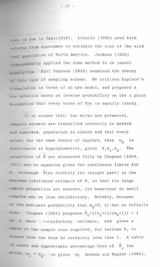
o.r>MF. conditional distributions

Poissnn Variablesand x2 are independent Poisson random

variables with means and ©2 respectively, then

Lt Ls readily shown that the distribution of

conditional on y = x 1 + x 2 is binomial, namely

Conversely, if x^ and y are a pair of random

variables such that the conditional distribution of x^

given y is binomial with parameters y and p, then

y is a Poisson with mean Ap.

Multinomial Variables

Let x1,x2,...,xk have a multinomial distribution

then the joint marginal distribution of x^ and x2 is

f(x15 |y) = (y )p 1 q 2X,

where P 0 -j/( 01 + 0 2 ) .

f(x-^,x2, . . . ,X^)

i=±

■1 (X}, x2 )x1 !x2!(n-x1-x2)!

n!

If y - x i + x 2 then y has probability function,

25 -

f(y) = (y) ( Px+P2 )y ^1-Pi"P2 ) y

and the condition probability function of x= X-, + x0 isgiven y 1 2

pl •xi 2pl+p2 P1 +p2

CHAPTER TWO

t.ttF.RATURE review and statement of the problem

2#1 literature review

We shall start by giving the history of a closed population (single marking). The structure is extremly simple. A closed population of unknown size N is under study, n^ individuals of which are marked and released. From this population, a sample of size r i2 is taken at a single instant over a period of time, m 2 of which are found to be marked.

The first recorded use of this technique is due to Laplace (1786). He estimated the population of France by recording the number m 2 , of births in some parishes of known population n 2 , whose names were recorded amongst the n^ names in the birth registrations for the whole country. Petersen (1886) first suggested the use of records of the proportion of marked indivi­duals in the study of fish population. When we spread the labelled fish over the whole fishing ground, we may with some reason suppose that, proportionally,"as many of unlabelled fish which are living there will be caught as those that are labelled." Then intuitively the proportion of marked individuals should be the same in the sample as in the population, that

m2^n2 = ni/N. This leads to the Petersen estimateA

^ = nln2^m2* The recorded use of Petersen's

27

idea is due to Dahl(1919). Lincoln (1930) used bird returns from sportsmen to estimate the size of the wild fowl population of North America. Jackson (1933) independently applied the same method to an insect population. Karl Pearson (1928) examined the theory of this type of sampling scheme. He critized Laplace's formulation in terms of an urn model, and proposed a new solution based on inverse probability on the a prior assumption that every value of N>n is equally likely.

If we assume that: the marks are permanent, sampled animals are classified correctly as marked and unmarked, population is closed and that every animal has the same chance of capture, then m2 is distributed as hypergeometric, given N,n^,n2 . The

Aproperties of N are discussed fully by Chapman (1948, 1951) and an equation given for confidence limits for

A

N. Although N(or strictly its integer part) is the maximum likelihood estimate of N, so that its large sample properties are assured, its behaviour in small samples may be less satisfactory. Notably, because of the non-zero probability that m2=0, it has an infinite bias. Chapman (1951) proposes Nc= [ (n^ + 1)/(m2+l) ] ~ 1 as a more satisfactory estimate, and gives a table of the sample size required, for various N, to ensure that the bias be certainly less than 1. A table of exact and approximate percentage bias of N^ for N=100, n1 = n2 , is given by Robson and Regier (1964).

28

Chapman shows also that, for values encounteredA„ N has a smaller expected mean s<in practice,

A

jrror than N.

mean square

However, since N is usually fairly large, the

hypergeometric distribution may be approximated by a binomial, Poisson, or normal distributions. Chapman

(1948) suggest the following criteria for approximating

the hypergeometric distribution by binomial, Poisson,

and normal distributions:

for n 2 < 500: m2/n2 < 0.1: Poissonm2/n2 > 0.1: Binomial

for 500<n2 1000 : m2/n2 < 0.075: Possonm2/n2 > 0.075: Normal

for n2 > 1000: m2 < 100 or m2/n2 < 0.05Otherwise : Normal.

Robson and Regier (1964) use the normal approxi­mation when N>100. Admas (1951) suggests the use of the Poisson approximation when N>_25, and provides charts for reading off confidence limits, based on theory developed by Ricker (1937). Since Poisson and normal distributions are themselves approximations to the binomial, it is usual for theoretical discussion to be based on a binomial distribution for the number of recaptures of marked animals. Confidence intervals for estimates from the binomial distribution may be obtained by reference to t e charts by Clopper and Pearson (1934). The use of

approximations was also suggested by DeLury (1951),normal

29

who derived confidence intervals for N on the assumptionthat m, is normally distributed with mean n ^ / N ,

2

variance (n ^ / N ) (l-n1/N): thus (n±n2/{Sm2( l-m2/n2 )} ,n n /{m -l.96/m2(l-m2/n2 )}) is the 95 percent confidenceinterval for N. Gaskell and Parr (1966) introduceBayesian methods to the binomial model. Having shownthat what they regard as the ideal prior distributionof N, f(N) a NB e-av, leads to intractable algebra, they

2consider f(N) constant and f(N) 1/N as ’extreme' prior distributions 'between' which their optimal prior

A

must lie. For these distributions N = n ^(n^-l)/(m^-2) and n-^n^ + l)/!! respectively, so that they recommend the

A

use of the 'intermidiate' N=n^n^/(m^-1). Questions of whether the prior distributions are really 'extreme', and what inference is to be drawn if one recapture is made, render this estimate unacceptable (Cormark-1968); whatever the merits of Bayesian inference.

Bailey (1952) shows that N=n^n2/m2 has a positive bias of order 1/m^. Thus in long run the size of thepopulation will be overestimated. He proposes (1951,1952),

/\the modified estimate NB=n1(n2+l)/(m2+l) with bias of ordere 2> its variance is given by n^2( n2 + l)( n2~m2 )/(11 + 1 ) (1112+2 ) .

/\

The difference between and Nc is negligible.

Bailey suggests an estimate = n2(n^+1)/m2-l, with variance (n^rr^ + l) (N+l) (N ; n2 ) / (m2+2 )m2 if sampling without replacement is assumed. Assuming binomial model, nln2//m2 an unbiased estimate of N, with variance

30

N(N-m )/m2 which may be estimated unbiasedly by 22 (ru-m0)/m0 (m9+l) (Chapman (1952)). Chapman uses

**1 l l 2 ' 2 ^ ^ ^

the normal approximation to set up confidence intervals and tests for N, but suggests that the Poisson approxi­mation will be more useful if both and n^/N aresmall. For inverse sampling from a Poisson distribution

2it is well known that 2n^n2/N is distributed as X with 2m2 degrees of freedom. This well-tabulated distribu­tion permits confidence limits for N to be easily constructed.

Chapman (1952) shows that the inverse sampling method gives a more efficient estimate of N with less average effort than can be obtained by direct sampling. However, if the experimenter knows absolutely nothing about N, he may, by an improper choice of n^,n2, give himself a sampling scheme which in practice cannot be carried out: the variation is extremly large. This difficulty may be partly overcome by devising the inverse sampling to stop when a predetermined number of unmarked individuals have been caught. Chapman (1952) shows that no strictly unbiased estimate exists:A

N=n2((n1 + 1) / (m2 + l)} -1 has a bias less than unity for samples for which n ^ n ^ n ^ ) > N log N. The variation in N is much reduced by this scheme. Despite these theoretical advantages, inverse sampling has been little used in practice (Ricker, 1958). Czen Pin (1962) shows that, for a loss function of the form (N-N) /N , a

31 -

minimax estimator of N exists, given by n ^ / ( m 2 + l) + b,H f n is the smallest allowable value of N) where ir-*-

N (1- A l - m 2 / n ”) / (m2 + l) < b <: N q (1+ /l-m2n1/N0) / (m2+l) .^ubrzycki (1963) shows that such estimators withh < N (nu+1) are inadmissible.D o 2

The decision as to when to stop sampling may be made according to a rule other than a fixed n2 and m2 discussed above. Chapman (1954) considers a series of samples of predetermined sizes n^(which are not returned to the population), sampling being stopped as soon as a total number, m, of marks have been recovered. If N is large, and a Poisson distribution is assumed,AN = n1Zni/m2 is asymptoticatly a minimum variance

2unbiased estimator with variance N /m2. Knight (1965) discusses the feasibility of estimating 1/N if sampling stops when either m2 or n2 attain a pre-assigned value, whichever happens first: he gives rules for choosing these values in such away that the variance of 1/N is less than any assigned value.

One theoretical difficulty in estimating N is that the distribution of n^n2/m2, or the modifications proposed by Bailey or Chapman, is far from symmetrical. Thus the confidence limits obtained from Clopper-Pearson curves

be biased. One way out of this difficulty is to estimate the reciprocal 1/N. As Leslie (1952) point out, under the binomial assumption m2/n^ is an unbiased maximum

32

ljkelih°ocl estimate of 1/N, and the confidence limits/s

may he obtained for 1/N by Clopper-Pearson charts or normal approximation. Since the distribution of

A

1/N is more symmetric than that of N, this procedure should lead to confidence limits of N less baised than the methods described earlier in this section. One disadvantage of using 1/N is seen if sub-populations are estimated separately, and it is desired to add the estimates together.

If we assume that (i) there is neither recruit­ment nor immigration both of which affect unmarked animals only and death and emmigration affect marked animals equally and (ii) if there exists strata within the population such that, by size, behaviour or any other variation, different strata have different chances of recapture, then the marked animals belong to these strata in exactly the same proportions as the occurence of the strata in the whole population, then the estimates considered above retain their properties ol consistency and unbiasedness. However their variances are now dependent on further unknowns, death rates and strata sizes, about which the investigation provides no information. Chapman (1952) shows that the modification is slight unless mortality is excessive. Chapman and Junge (1956) assert that, under the binomial assumption, a death rate, identical for marked and unmarked animals,does not affect the variance of the Petersen estimates. This is, however, true only if both marked and unmarked

33

populations are large enough for the death rate to be truLy deterministic. With death rate (l-(f>) , the population to be sampled must be assumed to contain N$ members of which n<|> are marked.

Chapman and Junge (1956) have investigated a possible modification of the last assumption. The population is assumed to consist of a number of distinct strata which do not mingle uniformly. These may be 'tribes' differentiated by geographical locality It is known to which stratum any sampled individual belongs at the moment of sampling, but its history is unknown unless it is already marked. Estimates are now required for population migration between strata as well as for total population size. Using suffixes i,j to represent the strata at the times of marking and sampling respecti-

A

vely, Chapman and Junge show that Z N . w h e r e. j 3

A

Z nKj N *j^n *j=ni for all i, is a consistent estimatorof N .. if it is assumed that sampling is random withineach stratum, individuals in each stratum are properlymixed after moving, individuals move independentlyone stratum to another, and the probability of such amove is independent of marking. (A suffix replaced bya# (period) has been summed over: thus, for example,while nr is the number of individuals marked instratum i, recaptured in stratum j, m.j = £ nr . is the

i -*total number of individuals recaptured in stratum j ). Under the same assumptions neither the standard Petersen

34

estimate nor an estimate Z Z nj -mij/m± *mj , proposedarlier for this situation by Schaefer (1951b), isonsistent unless the assumption that there exist strata

within the population, such that by behaviour, size orary other variation, different strata have differentchances of recaptures holds strictly. Estimates arealso given for migration between strata:/\ am = m N..N. ./n..n. .. This situation was studied ij ij i J 1 Jfurther by Darroch (1961). If there are at least as many strata in the population at the time of marking, as at the time of recapture, maximum likelihood estimates are obtained without any assumption as to the movement of unmarked animals. If not, then it is necessary to assume that unmarked animals move between strata with the same probabilities as marked ones. If the movement of individuals is not independent, the estimate remain consistent.

More important than these theoretical problems of trying t.o extract from the data, under the assumptions, the last scrap of information, is the problem of how departures from the assumptions affect the estimate of N, and how, if at all, the estimate may be adjusted to allow for such departures. Indeed, as Schnabel (1938) says: "since the assumptions of random sampling and constant populations are only rough estimates to the actual situation in taking fish census, small differences between the results of various methods are not important."

35

Be ort on actual experiments with fish populations 'llustrating the breakdowns of these assumptions which occur in practice will be mentioned later.

Rupp (1966) has pointed out that the Petersen procedure can be regarded as a particular instance of a survey removal method of estimating population size.In survey-removal study, originally suggested by Kelker (1940, 1944), the change in ratio of the observed frequencies of occurence of two distinguishable classes of individuals, before and after a period during which known numbers of the two classes are removed from the population, provides information about the size of the population if markedly different numbers are removed from the two classes. Theory of this method, allowing for mortality is developed by Chapman (1954), Lander (1962), Hanson (1963) and Chapman and Murphy (1965).In Petersen-type study the initial ratio of marked: unmarked is zero. The final sample ratio is m^/(n2_fTO2 >“ni marked animals having been removed before the final sample. Paulik and Robson (1969), in a unified treatment of the methods, study the effect of N of an unobserved removal

Cm> Cu animals from the two classes during the period before the final sample. These C , C^ cover mortality, immigration, and emigration (not necessarily the same for each class), and this formulation permits any knowledge of these unobserved removals obtained from other sources to e used in the estimation of population size.

36

The effects of recruitment may be eliminated in some hv restricting the counts to suitable age groups -

if these are recognizable and non-overlappJ ng (Ricker (1958)).

Even if age 9rouPs overlap, subsidiary information on

growth rate can be used to eliminate the effect of recruitment. The possibility that the process of marking

in itself introduces an extra cause of mortality to marked fish may be investigated by using different types of mark, if one of these involves more mutilation than another, and

yet both types are recovered equally in the subsequent sample, this provides evidence that marking does not

contribute directly to the mortality. This does not

cover additional mortality due to purely handling the animals, which often have to be removed from their natural environment.

The assumption that there is no loss of marks, may

be investigated by fixing two marks to some individuals.

If it is assumed that losses of single marks are independent

Lhen the number of individuals in the sample which havelost none or one of the two marks fixed on them provides

information on the rate of loss. Thus, if all animalsreleased bear tow marks and are recovered still bearing

both marks, m with a loss of one mark, the loss rate smay be estimated by m / (m +m^), and the population size

u s s Dby 4 mDm s.n2/(2mD+ms) 2. A more general model than this

is examined by Gulland (1963). Data on plaice recorded

37

b Beverton and Holt (1956) suggest that the rate of detachment of external tags increases with time ini­tially (with increasing wear), but then decreases (as the tags become imbedded).

If the recapture sampling is continued over a period of time, any dilution of the population - by recruitment or immigration - should become apparent through a progressive decrease in the proportion of marked animals in the recaptured samples. Jackson (1937) in his 'positive method' adopted this procedure, and Bailey (1951) provides a mathematical formulation by which dilution, if assumed to have a specific mathe­matical form, could be estimated. Parker (1955) sug­gested plotting, as a function of time, m/n, or log(m/n) or arcsin (/ m/n ), whichever provides the best straight line, and was more satisfactory.

Knowledge of the effort expended in sampling the population allows the estimate of the population size to be obtained in a different way, since the numbers obtained per unit effort will diminish in successive samples (Leslie and Davis, (1939)). If the effort is the same at each sample, the expected catch in the sample, Etci], is related to the probability p of an individual being caught, by the relation E[CL] = Np(l-p)^ ^ . A

38

wei hted regression of log Ci against (log(Np)+(i-1)log p) ; estimates of p and N. Moran (1951)pointedg i v.. + r ’ s are not independent and derived maxi- out tnai '■'i

mum likelihood estimates for N and p. Skellam (1962) proposed direct numerical extrapolation to the curve of catch against time, suggesting that a transformation of the time variable t to a form b/(b+t) (where b is arbitrary) enables the extrapolation to be carried out more accurately. Chapman (1954), following DeLury (1951), proposes an unweighted regression of - inthis case the catch per unit effort - on K^, the total catch removed before the ith sample. This give

nN = K - C (K.-K) /IC.(K.-K). A comprehensive study Jof these removal methods is given by Zippin (1956).Chapman shows further that this idea can be suitably combined with capture-recapture experiment with a single release of nQ individuals, and successive periods of recapture yielding n. individuals of which no are marked. If n^ and no given n^, are both assumed to have a Poison distribution, maximum likelihood equations are given for N and q the probability that a unit of effort captures one member °f the population, in terms of the efforts f. expended (Chapman (1954)).

The Petersen estimate or Lincoln Index, perhaps modified for bias, has been much used as providing a simple and intuitively reasonable estimate of population

39

However, the universal lack of faith in the

assumptions together with the lack of internal evidence

as to their applicability led to consideration of models

for more complicated sampling procedures.

Discussion of the study of a closed population

by the use of marked individuals would be incomplete

without mention of some proposed methods based on the

number of times individuals are recaptured. Craig (1953)

suggested that if the total sampling period is subdivided

into a large number of short intervals and each individual

is equally likely to be caught in any short interval,

the number of recaptures should have a Poisson distribu­

tion, truncated at zero since it is not known how many

individuals are never captured. From this, N and the

Poisson parameter can be estimated by maximum likeli­

hood or by moments. Darroch (1958) shows that Craig's

use of truncated Poisson distribution can not serve

as a probability distribution of any capture-recapture

experiment since it implies that both the total effort

expended and the number of different individuals seen

be fixed in advance, was impossible. Taylor (1966)

reports that for bird population the number of times

an individual is recaptured is not well fitted by a

trancated Poisson distribution. He suggests a negative

binomial distribution.

Me Donald and Palanacki (1989) considers the

problem of estimating the size of a small population

40

ased on the results of a certain type of capture- recapture experiment. They give seven methods of constructing confidence intervals for the population

Among these methods is the 'adhoc' method which for N = tends to give actual confidence levelswhich are close to the desired level and tends to give shorter intervals than the other methods when the probability of capturing individuals is small.

We now consider a situation where marked animals are released into the population on more than one occasion. As with Petersen method described earlier these marked animals are usually themselves samples from the population under study, but this need not be the case provided due assumptions about marked and unmarked individuals, are satisfied. The earlier studies of this situation took no account of the possibility that a particular individual may be recaptured on more than one occasion. At sampling time i, i = 0,l,2,...,k, the data recorded are n^, the size of the sample, and nr , the number of previously marked animals in the sample.Ihe (n^-m^) unmarked individuals are then marked and aH the returned to the population. The first sample serves only to provide a pool or n (=M1) marks ln the Population. There are k subsequent recapturesamples.

41

The first study (Schnabel, 1938) assumed thatthe total number of marked animals in the popula-

1 'tion immediately before the ith sample in taken, are known parameters of the population. The situation is then identical with a series of Petersen estimates which have to be combined to yield a single estimate of the population size N. The situation remains to decide with what weights the estimates should be combined. Under the assumption of binomial sampling on each occasion, Schnabel (1938) proposed the estimateAN = (En^nr )/Enr as an approximation to the solution of the maximum likelihood equation:

(n.-m.)M.Em. = E --— —1 (N-M.)l

buL gave no consideration to the precision of her esti­mate. If M./N is small, and m. is assumed to be al l

APoisson variable, N is the exact maximum likelihood estimate, Schumacher and Eschmeyer (1943) proposed En^Ak /Effi M and suggested that its variance be obtained from the mean square error about the regression line mi^ni a9ainst M.. The estimate of variance has the advantage of referring to 1/N, which is more symmetri- cally distributed than N itself. Hyne (1949) proposed e same method, apparently independently of Schumacher and Eschmeyer, commenting that it has an advantage over

42

the removal method, in that it is not so severely upset by a day-"to-day fluctuation in the probability of capture. The different wei9 ^tings for each point on a graph of

/n against n through the origin which are implied by1 1

the various estimates were studied by DeLury (1958).The weights for the maximum likelihood solution are

A

n N/n (1 -n.j/N) those for the Schumacher and Eschmeyer2 tsolution, preferred by DeLury, are simply n. Ricker(1945b) asserts that Schumacher and Eschmeyer's estimateattains maximum efficiency when half the population ismarked; Schnabel's maximum occurs when a negligible

proportion is marked. They have equal efficiency whenthe proportion of marks is 1/4. In an earlier paperDeLUry (1951) had given an iterative solution for themaximum likelihood equation. Using Schnabel's estimateas a first approximation, a new weighted estimate •EW.n.M./EW.m., is constructed with weights

= 1/(1 - M^/N). Gilbert (1956) suggests thatthe difference between the hypergeometric and binomialdistributions can be allowed for by dividing each termin the binomially based likelihood equation by afinite population factor(1-n^/N). Thus instead ofsolving the equation E(m.n .—Nm^)/ (N^-M^) = 0, one

isolves the equation E(M.n .-Nm.)/(N-n^) (N-M^) = 0.

ismall example gives results very similar to the

43

binomial model.

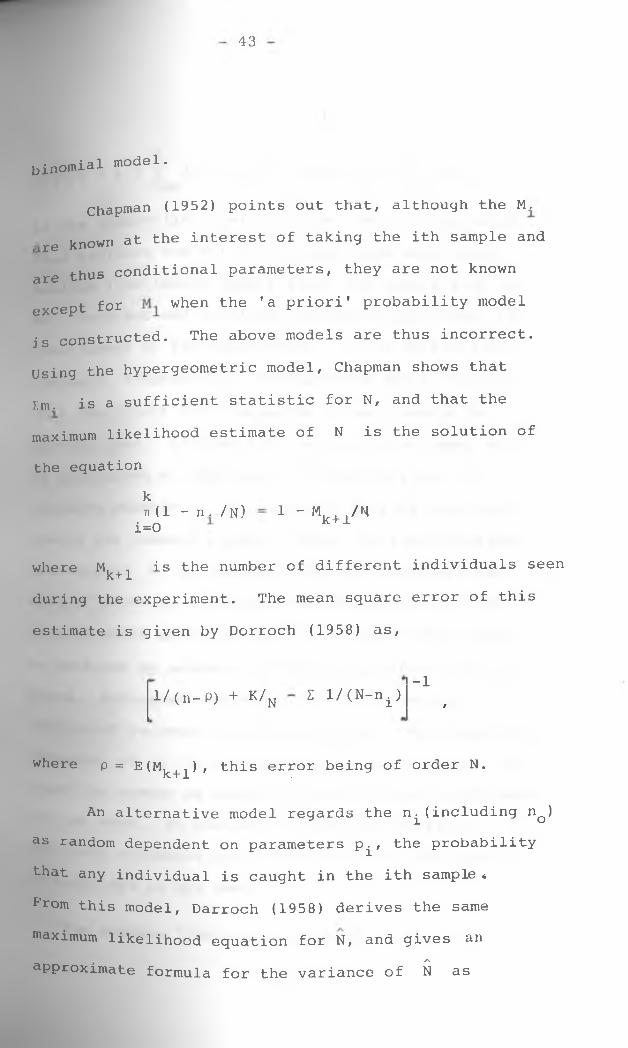
Chapman (1952) points out that, although the Nh

re known at the interest of taking the ith sample and are thus conditional parameters, they are not known

except for when the 'a priori' probability model

is constructed. The above models are thus incorrect.

Using the hypergeometric model, Chapman shows that

j;m. is a sufficient statistic for N, and that the

maximum likelihood estimate of N is the solution of

the equationkn (1 - n . / N)

i=01 - M /Hk+r H

where M, , is the number of different individuals seen k+1during the experiment. The mean square error of this

estimate is given by Dorroch (1958) as,

1/ (n- P) + K/n X l/(N-ni)-1

f

where p = E(Mk+1), this error being of order N.

An alternative model regards the n^(including nQ) as random dependent on parameters p^, the probability

that any individual is caught in the ith sample «

From this model, Darroch (1958) derives the same

maximum likelihood equation for N, and gives anA

approximate formula for the variance of N as

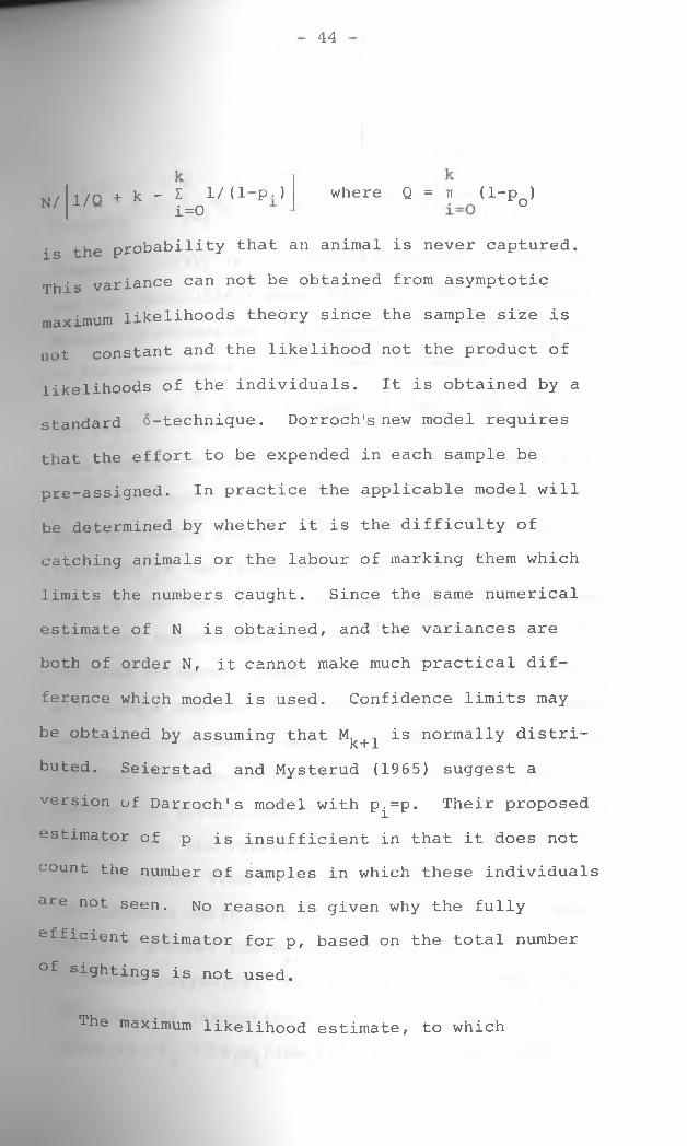
44

N/ 1/0 + k - £ 1/(1 p,)i=0

where Q = tt (l-po)

is the probability that an animal is never captured.

This variance can not be obtained from asymptotic

maximum likelihoods theory since the sample size is

not constant and the likelihood not the product of

likelihoods of the individuals. It is obtained by a

standard 6-technique. Dorroch's new model requires

that the effort to be expended in each sample be

pre-assigned. In practice the applicable model will

be determined by whether it is the difficulty of catching animals or the labour of marking them which

limits the numbers caught. Since the same numerical

estimate of N is obtained, and the variances are

both of order N, it cannot make much practical dif­

ference which model is used. Confidence limits may

be obtained by assuming that M^+1 is normally distri­

buted. Seierstad and Mysterud (1965) suggest a

version uf Darroch's model with p^=p. Their proposed

estimator of p is insufficient in that it does not count the number of samples in which these individuals

are not seen. No reason is given why the fully

efficient estimator for p, based on the total number °f sightings is not used.

The maximum likelihood estimate, to which

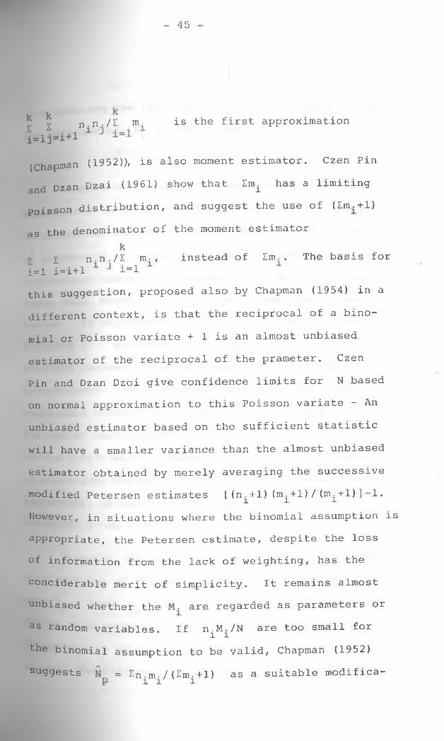
45

n.n./£ m. is the first approximation

(Chapman (1952)), is also moment estimator. Czen Pin

and Dzan Dzai (1961) show that Znr has a limiting Poisson distribution, and suggest the use of (Znr+1)

as the denominator of the moment estimator

this suggestion, proposed also by Chapman (1954) in a

different context, is that the reciprocal of a bino­

mial or Poisson variate + 1 is an almost unbiased

estimator of the reciprocal of the prameter. Czen

Pin and Dzan Dzoi give confidence limits for N based

on normal approximation to this Poisson variate - An

unbiased estimator based on the sufficient statistic

will have a smaller variance than the almost unbiased

estimator obtained by merely averaging the successive

modified Petersen estimates [(n^+1)(m^+1)/ (m^+1)]-1.

However, in situations where the binomial assumption is

appropriate, the Petersen estimate, despite the loss

°f information from the lack of weighting, has the

conciderable merit of simplicity. It remains almost unbiased whether the are regarded as parameters or

as random variables. If n^NL/N are too small for

the binomial assumption to be valid, Chapman (1952)

suggests = Zn-^nr/ (Enr+1) as a suitable modifica-

kZ n.n,/Z nr,

i=l i=i+l 1=1instead of Znr. The basis for

46

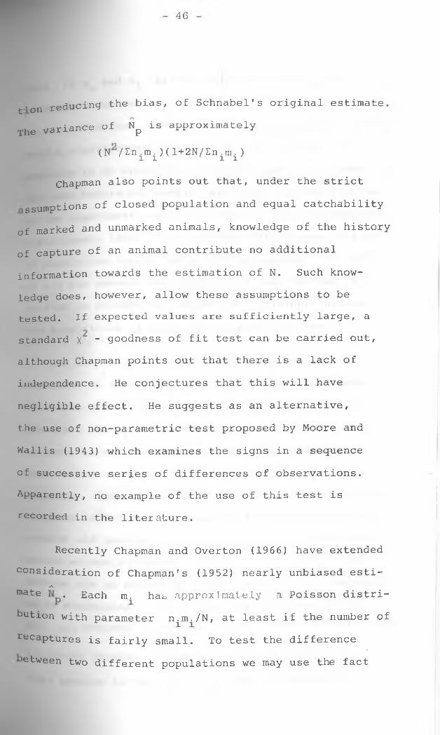
t ’on reducing the bias, of Schnabel's original estimate

The variance of Np is approximately

(N /fnim i)(l+2N/fnim 1)

Chapman also points out that, under the strict

ssumptions of closed population and equal catchability

of marked and unmarked animals, knowledge of the history

of capture of an animal contribute no additional information towards the estimation of N. Such know­

ledge does, however, allow these assumptions to be tested. If expected values are sufficiently large, a

standard X “ goodness of fit test can be carried out,

although Chapman points out that there is a lack of independence. He conjectures that this will have

negligible effect. He suggests as an alternative,

the use of non-parametric test proposed by Moore and

Wallis (1943) which examines the signs in a sequence

of successive series of differences of observations. Apparently, no example of the use of this test is

recorded in the literature.

Recently Chapman and Overton (1966) have extended

consideration of Chapman's (1952) nearly unbiased esti-A

mate . Each nr has approximately a Poisson distri­bution with parameter n.^nr/N, at least if the number of

recaptures is fairly small. To test the difference

etween two different populations we may use the fact

47

-if x and x. are Poisson variates, x is a that, 11 Ao 1 oinomial variable for fixed (x^+x^). An example based

n data of Nelson (1960) illustrates the manner in which

uch a significance tests may be carried out. It is

possible to do appropriate calculations on the power of

the test before any samples are taken so that the size

of the experiment required to detect, with appropriate

significance level, a pre-assigned difference in size

of population can be calculated beforehand. In view

of all the assumptions required, I doubt whether it

is wise to attempt to discuss the difference between

two populations in terms of a significant test.

As in a single stage census, sampling may be

continued at each stage until a predetermined number

of marked animals have been captured. The m^ are

fixed and the n. are random variables. An unbiasedlestimate is now easily found, being the unweighted

mean of the corresponding estimates from the inverse

sampling. Thus, N^l/KZCn^+l/rrK-l), with approximate

variance fN2E1/nK }/k2 . Chapman (1952) derives these results and goes on to discuss how to choose the para­

meters at one's disposal, n^,k,m^ ....... ,mk*obvious aim at achieving a fixed precision of estimation

while minimizing the effort expended, minimizing kE(E n.) subject to constant 5 /N, leads to a very complex

i=0 1algebraic problem. Chapman provides guidance in

this problem in the form of a table of properties

48

f a number of simple designs. Unfortunately interesting

cases with small iik break the mathematical assumptions

nd so cannot be considered. An increasing sequence of

m spreads the effort most evenly; constant seems

to provide the maximum precision for the same expected sample size.

Since direct censuses contain the awkward possi­

bility that not enough marked animals are captured to

permit reasonable estimates of N, and inverse censuses

have a similar physically imposed restriction, namely,

that it may not be possible to continue sampling until

the pre-assigned number of marked animals have been

caught, it is clear that optimal sampling procedures

must be sequential. Urn models for different sequential

schemes - one at a time, several at a time, single and

multiple markings - were introduced by Cox (1949).

Chapman (1952) considers in the direct case, the number of recapture samples k as a random variable to

be determined by the course of the sampling. He takes

np as fixed. Under the assumption that the m^ are

Poisson variates, a standard type of sequential

probability ratio test can be constructed. For any

valid study of optimality and expected number of samples

required to be taken the itk have to be independent, a

consideration not satisfied in this case. Sequential

aPproach was extended by Goodman (1953). A series of

49

samples predetermined sizes are to be drawn,

amplin9 to stop as soon as a total of m marked indivi­duals has been captured. A further extension by

Chapman (1954) did not restrict the replacement of

marked individuals in the population to those capturedin previous samples. Chapman showed that 2 En^M^/N

2is asymptotically distributed as X with 2m degrees2of freedom, so that Zn^Nh/m with variance N /m, is

the asymptotic minimum variance unbiased estimate of

N. Darroch (1958) considers a special case of Goodman's

sequential census in which each sample consists of a

single individual. For this case a unique unbiased

estimator, with minimum variance, exists for N. If

n samples have to be taken to achieve the recapture

of m marked individuals, the estimate is given by

the ratio o /a -i where as = Ar (os)/r '. *

a Starling number of the second kind. Other stopping

rules for this one-at-a-time census have been considered

by Samuel (1943). He suggests as a working approximation

to Darroch's estI mate the value n/w, where w is the

solution of the equation (1-e W)/w = (1-m/n) . Tables°f the function (1-e w )/w are given, for example, by Pearson (1934). Boguslavsky (1956) discusses estimation

N for small populations in which a number of succe­

ssive observations have yielded only marked animals.

50

Overton (1965) discussed the modifications to be

ade to the Schnabel estimator when known numbers of nimalS/ both marked and unmarked, are removed from

he population during the course of the experiment.This removal may be deliberately caused by the experi­menter or the result of accidential damage to the sampled individuals. The modification takes the form of a term, which has to be computed iteratively, and is then added

to the usual Schnabel estimator.

The assumptions under which the above theory of

Schnabel type estimators is valid are the same as for

the Petersen case. Since the sampling is usually

continued over a longer period than the Petersen-type

studies, Ricker (1958) considers the recruitment and

natural mortality (and fishing mortality if the popu­

lation is subject to this pressure) as errors of

special importance. Undetected natural mortality

seriously affects the multiple sample census (Chapman

(1952)). One method of testing for natural mortality,

particularly adapted for entomological studies, is to

compare for any one recapture sample the Petersen

estimate obtained by considering only individuals

marked on different occasions (Southwood and Saudden

(1956)). By considering the multiple census as a time

sequence of single cencuses, each of which gives an

51

stimate of the population size at that time, any change

in the population over time may be investigated. This

is the basic principle of the models to be considered

in the later sections of this dissertation, which includes

mortality and recruitment as parameters. Mortality

causes the population to decline, and thus the Schnabel

estimate of the population size will be less than the

Petersen estimate from the first sampling. This was

used to measure mortality by Debury (1951). With

greater sophistication, natural mortality may be estimated

as that which eliminates any time trend from succesive

daily estimate of 1/N (Ricker (1958)). This type of

estimation is closely analogous to the analysis of

catch curves to give estimates of mortality.

Fienberg (1972) considers the problem from a

different angle. The resulting data can be put in a

form of an incomplete 2 contingency table, with one

missing cell, that displays the full multiple recapture

history of all individuals in the population. Log

linear models are fitted to this incomplete contigency

table and the simplest possible model that fits the

observed cells is projected to cover the missing cell, thus yielding an estimate of the population size.

If sampling contines over an appreciable period

°f time, the population cannot be assumed closed. Other

Population parameters for recruitment and mortality (and

52

ssibly immigration and emigration) must be included in

the model. What is meant by an appreciable period of time

depends on the population under study. Insect studies

with daily samples for a week have to allow for mortality. Surveys of large mammals over period of a month may not.

The early models assumed a deterministic death rate, constant over different periods. With death rates (1— 0) ,

N individuals become exactly <}>N. The simplest estimate

of mortality over a period during which dilution may

be ignored is the ratio of two Petersen or Schnabel estimates of population size at the beginning and end

of the period.

In a series of papers, Jackson (1937, 1939, 1940,

1948) suggested two sampling schemes which he termed

'positive' and 'negative' methods. The positive method

is release on a single occasion, a large number of

marked animals, recapture (and re-release) being effected

frequently on several occasions. The negative method called for the release of marked individuals on several

occasions. The number of recaptures being noted only at

one final intensive sampling. This second method was

deemed most suitable when unskilled workers were used to carry out the marking. Jackson stated that either the

^ rst capture or the recapture should be carried out non-

solectively since 'dispersal ....might not be complete in

the Period between marking and recapture, or individual

53

lies might return to places to which they were speci­fically attached'. Jackson tried to standardize the

a^piing effort by analysing not the basic number m

0f recaptures, but yQ1 = m ^ / n ^ , where mQ1 is the

mnber of individuals among the n^ caught in week 1,

which were marked in week 0 when nQ were caught.

The ideas behind the negative method is that the

samples released early have been exposed to natural mortality for longer periods than samples released

at a later date, and therefore will be represented

by fewer individuals in the recapture sample. The

death rate can be estimated and used to give an estimate

of the number of marked animals alive in the population

at the time of recapture sample. An estimate of the

population size at this stage follows as usual fromA

N=riin^/m2 . Since it is the population at this final

time which is being estimated, immigration during the

period of sampling is an integral part of the popula­

tion. There is no problem of allowing for it. A very

simple example is given by Ricker (1944). If s1,S2

fish are marked and released immediately before the

fishing season in two successive years, and during the

second year's fishing, m 12, m22 resPectively of the si' s 2 are caught, then the mortality between the years,

inclusive of that due to fishing in the first year, is

estimated by s2 m 12/s^m^. In the positive method

54

when all animals arc re Leased in week, 0, the y

will decrease with time on account of dilution 0f the

population by unmarked animals. This curve may be

extrapolated to time 0 to provide an estimate of

population size, and the rate of fall of the curve

gives an estimate of dilution rate 3. Jackson's

estimate of population size, which he attributes

to Fisher is

{y01+ y02 + .... + y0(k-l)}- {

02 y0ky01+ '“ +yO(k_2)}

and a variance formula, due to W.L. Stevens, is also

quoted. The dilution rate is estimated by

(y01+--- +yok-l)/(y02+ --•+y0k)' If 3 does not aPPearto be constant, Jackson later (1940), suggested using

the estimate provided by YQ2/y01 Perf°rm the extrapolation to provide an estimate of the population

size. Identical consideration apply to the negative

method.

Bailey (1951) comments on the lack of proper

weighting factors in Jackson's (1937) estimates, and

develops a maximum likelihood solution. For the 'negative'

method with recapture only on the final day, day k>

assuming a constant death rate (1-$), s.e ^1 v)(k-j)

°f the s. animals released on day j will be still alive.JThe likelihood of the parameters 4>, is thus proportional to

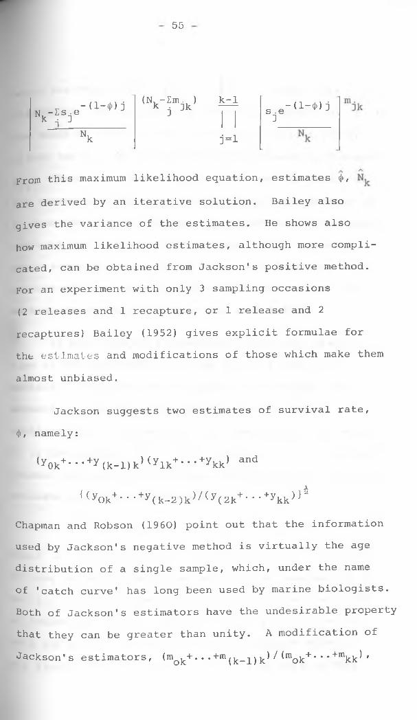
55

-(1-<J>) jNk - f j e

(N, -Em . ) 1- k j ]k C-]Ls .e_(1"l,>) j D

Nk j = l

From this maximum likelihood equation, estimates <J>,

are derived by an iterative solution. Bailey also

gives the variance of the estimates. He shows also

how maximum likelihood estimates, although more compli­

cated, can be obtained from Jackson's positive method.

For an experiment with only 3 sampling occasions

(2 releases and 1 recapture, or 1 release and 2

recaptures) Bailey (1952) gives explicit formulae for

the estimates and modifications of those which make them

almost unbiased.

Jackson suggests two estimates of survival rate,

<|>, namely:

(y0k+ '’,+y(k-1)J(ylk+ ‘'•+Ykk) and

{(y0k+ ' ’ •+y(k-2)k)/(y(2k+ - ' '+ykk)}4

Chapman and Robson (1960) point out that the information

used by Jackson's negative method is virtually the age

distribution of a single sample, which, under the name

of 'catch curve' has long been used by marine biologists.

Both of Jackson's estimators have the undesirable property

that they can be greater than unity. A modification of

Jackson's estimators, (m^* • • •+m (k-i) k ^ mok+ ’ * *+mkk^ '

56

hich was suggested by Heincke (1913), avoids this

difficulty, an< is infact an unbiased estimator of <j> in

the study of catch curve. To allow for variations in

effort the irt should presumably be replaced by Jackson's

v Chapman and Robson give a detailed discussion ofyij*the regression techniques behind graphical estimates of

(j) from the relation between the logarithm of the number

captured and the time since marking. These remarks

apply strictly to the 'catch curve' situation but have

considerable relevance to such techniques as used in

marking experiments, (Beverton and Holt (1956)).

In most recapture experiments the 'age' distribu­

tion of the recaptures - in the sense of time since

marking-is truncated at the upper and sometimes fairly

severely, since these experiments are not usually

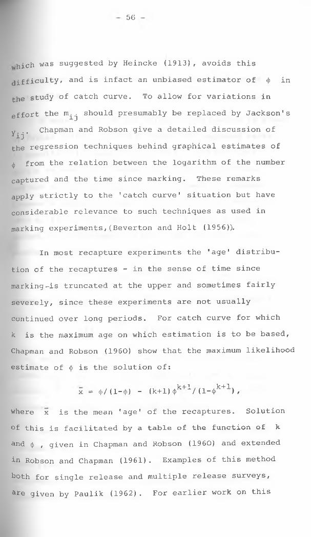
continued over long periods. For catch curve for which

k is the maximum age on which estimation is to be based,

Chapman and Robson (1960) show that the maximum likelihood

estimate of (j) is the solution of:

■\r i 1 k + 1

X = <|>/(l-<f>) - (k+l)(T -Vd-* ) ,

where x is the mean 'age' of the recaptures. Solution

of this is facilitated by a table of the function of k and (j) , given in Chapman and Robson (1960) and extended

in Robson and Chapman (1961). Examples of this method

both for single release and multiple release surveys,

are given by Paulik (1962). For earlier work on this

57

subject see Haldane (1955). An example is given by Murton (1966) .

A model based on the Poisson distribution is given

by Parker (1963). In this, removal of captured marks

is specifically taken into account. If there is a

single release of Mq marked fish into a population,

subject to constant absolute recruitment B- compare

Chapman's comments below - and instantenious mortality

rate x, from which samples of n^, of which m^ are

marked, are subsequently taken, then at time t, the

population will consist of

N e~xt - Z n. ex(l_t) + B(l-e"xt)/x ° i=l 1

among which the expected number of marked individuals

is... -xt tv1m x(i-t) M e - l m. e° i=l 1

If may be assumed to be a Poisson variable condi­

tional on m^, m 2 i ••• r mi_i and ni are taken as para­meters, N , x and B can be determined by iterative osolution of maximum likelihood equations.

Further entomological studies on similar lines to

Jackson's were carried out by Dowdeswell, Fisher and

Ford (1940, 1949) and by Fisher and Ford (1947). These

introduce a new method of grouping and displaying the

observation as in the form of a trellis diagram.

58

Releases on day Total recapturesf '0 1 2 3

Recaptures

on day "1 m oi n

2 m02 m12 n

<3 m03 m13 m23 n

4 m04 m14 m24 m 34 n

L* • • • • •

Totalreleases so si S2 S3 4

w

These m . . include all individuals seen on both day i and IDj. The average survival rate <j) is estimated from the

average time interval separating release from observed

recapture. From this, the population on day j is esti­

mated by n.m./M., where M. is an estimate of the number

marked animals alive at time j. The estimate given by

Fisher and Ford is M. = E s . (pJ , which counts each3 i=l 1

individual, at any recapture, as often as it has previous

marks. Using only the last previous recapture of each

mark would be more valid. No estimate of the precision

is available. The logic of this estimate of N is the

same, given <J) , as Jackson's estimate as derived by

Bailey (1951). A modification to Fisher and Ford's

59

calculation of available marked animals is given by

Macboad (1958) for the case in which recapture sampling

is continued until no hope remains of survivors being

caught.

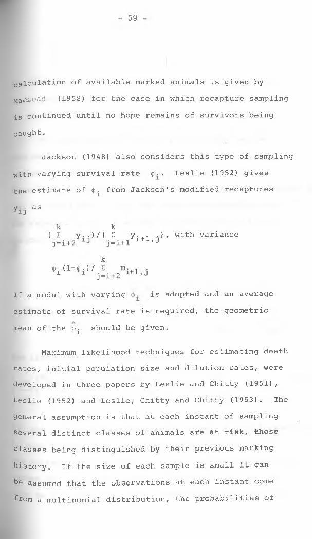
Jackson (1948) also considers this type of sampling

with varying survival rate <j . Leslie (1952) gives

the estimate of (f) from Jackson's modified recaptures

If a model with varying is adopted and an average

estimate of survival rate is required, the geometric

mean of the (f> should be given.

Maximum likelihood techniques for estimating death

rates, initial population size and dilution rates, were

developed in three papers by Leslie and Chitty (1951),

Leslie (1952) and Leslie, Chitty and Chitty (1953). The

general assumption is that at each instant of sampling

several distinct classes of animals are at risk, these

classes being distinguished by their previous marking

history. If the size of each sample is small it can

he assumed that the observations at each instant come

from a multinomial distribution, the probabilities of

as

ky..)/( £ y.,.. •) , with variance

n = -i+l 1 + ± ' J

k4>i (1-^i) /

60

the different classes being expressible in terms of the

basic parameters of the model. The overal likelihood

is the product of a set of such probabilities.

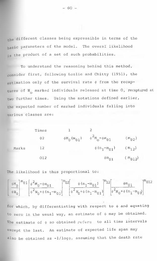
To understand the reasoning behind this method,

consider first, following Leslie and Chitty (1951), the

estimation only of the survival rate <J> from the recap­

tures of marked individuals released at time 0, recaptured at

two further times. Using the notations defined earlier,

the expected number of marked individuals falling into

various classes are:

Times i 2

02 4,M0(n,01) 4>2Mo-0m01 (m02 >

Marks 12 $ (ni-m0i) <m12>012 <Dm0 j ( m012

The likelihood is thus proportional to:

fo£-e-

•

moi 2<f> M0-4>m0i m02 ’4> (n^- ^ m12 <f)m0i

. *Mo.2<t> MQ+(p (n1-m01) 2<p Mq + cJ) (n1-mQ1) 24> Mq+(J) (n1-mQ^

for which, by differentiating with respect to $ and equating

to zero in the usual way, an estimate of <j> may be obtained.

The estimate of cf> so obtained refers to all time intervals

except the last. An estimate of expected life span may

also be obtained as -l/log<J>, assuming that the death rate

61

is not age-dependent.

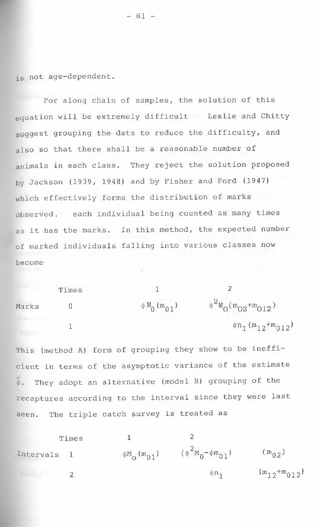
For along chain of samples, the solution of this

equation will be extremely difficult Leslie and Chitty

suggest grouping the data to reduce the difficulty, and

also so that there shall be a reasonable number of

animals in each class. They reject the solution proposed

by Jackson (1939, 1948) and by Fisher and Ford (1947)

which effectively forms the distribution of marks

observed, each individual being counted as many times

as it has the marks. In this method, the expected number

of marked individuals falling into various classes now

become

Times 1 2

Marks 0 (\>‘ m02+ITl012)

1 (})n1 (m12+m(

This (method A) form of grouping they show to be ineffi­

cient in terms of the asymptotic variance of the estimate

. They adopt an alternative (model B) grouping of the

recaptures according to the interval since they were last

seen. The triple catch survey is treated as

Times 1 22

Intervals 1 ^Mo^m01^ ^ M0-( ra01^ (m02^

<f>n12 (m12+m012 ^

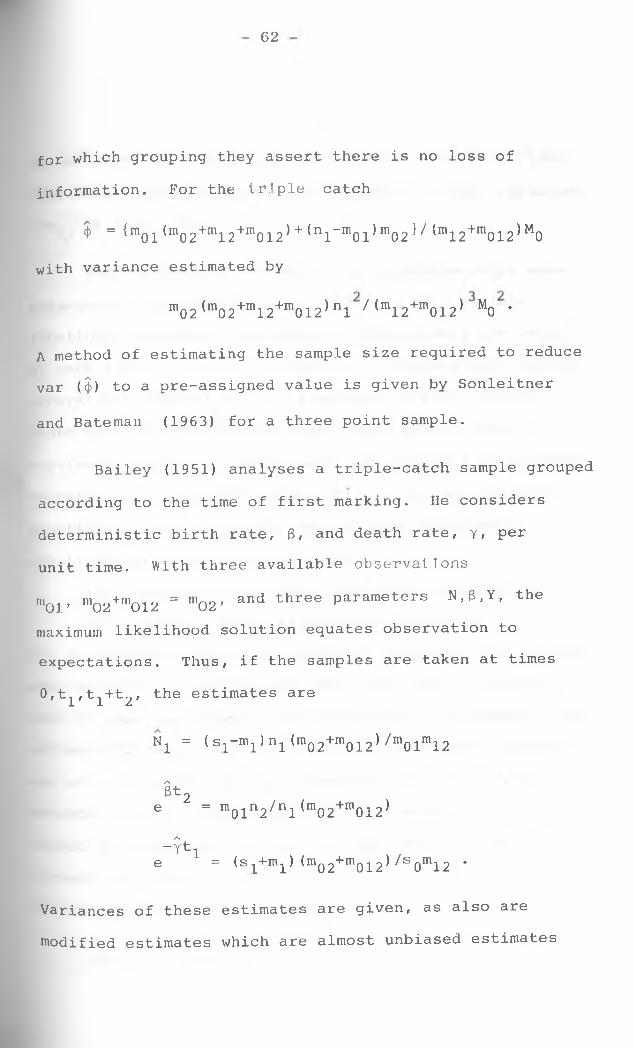
62

for which grouping they assert there is no loss of

information. For the triple catch

$ = {mQ1(mo2+m12+m012^+ nl-m01^m0 2 ^ ^ m 12+m012^M0 with variance estimated by

m02(m02+m12+m012*nl /(m12+m012) M0 *

A method of estimating the sample size required to reduce

var ($) to a pre-assigned value is given by Sonleitner

and Bateman (1963) for a three point sample.

Bailey (1951) analyses a triple-catch sample grouped

according to the time of first marking. He considers

deterministic birth rate, 3/ and death rate, y, per

unit time• With three available observat ions

m01> n'02+m012 = m02 * and three parameters N , (5, Y , the maximum likelihood solution equates observation to

expectations. Thus, if the samples are taken at times

0,t1,t1+t2, the estimates are

Ni = ( s-i -m^ ) nx (m02+m012)/m01m 12

§t2e = ni01n2/n1 (m02+m012)

A

"Ytle = (s- +m ) m o2+m0 1 2 ^ S 0m12 *

Variances of these estimates are given, as also are

modified estimates which are almost unbiased estimates

63

of variances of these estimates. Gaskell and Parr (1966)

from their Bayesian standpoint, recommend always replacing

l/mij by 1/(mij”1).

The problems of estimation of population size were

subsequently studied by Leslie (1952). The complete

likelihood function, including all the animals not caught

at each sample, has to be maximized. Classes were grouped

according to method B. For a population with constant

death rate and no dilution Leslie used the estimate of

survival $ from the earlier paper and obtained an approximate

estimate of N by substituting <j> for (p in the likelihood

equations. Leslie also derived maximum likelihood

equations for the populations with:

(a) constant death rate, but dilution occuring

(b) changing death rate and no dilution;

and he mentions a possible method of attack on the problem

when dilution is occuring and the death rate is varying

both in time and between different groups of animals. The

estimate of the population size suffer the same disadvant­

age of bias as the standard Petersen index and Leslie

extends Bailey's modifications to the general case. It

should be noted that dilution in these models - as in

Jackson and Bailey - is a function of the size of the

existing population.

Leslie, Chitty and Chitty (1953) develops the

64

theory further with particular reference to the problems

discovered during an extensive study on two small mammals.

An improved approximate method is used to derive estimates

from a method B grouping. Various tests were applied

to the data. The assumptions necessary for valid esti­

mation of the population parameters were found to hold

for one population but not for the other. He asserts

that reasonable, and useful inferences, may be deducible

about the sub-population of marked animals, even if

not about the population. The point is made again by

Pope (1963); "when only mortality rates are to be

estimated from marking experiments it is not necessary

to consider the whole population, but only the sub­

population of marked individuals". This is however, no

advantage if marking affects mortality.

Corbet (1952), using Fisher and Ford's method

estimated different survival rates for different periods

of experiment. He reiterates the warning to analyse

sexes separately because of their differential activity.

Coulson (1962) modified Bailey's tripple catch method

to allow the first recapture to be taken on the day of

release, this is necessar^ because of the short lifespan

of the animals studied. Wohlschlag (1954) applied Bailey's

method to a eontinouos experiment by dividing the study

into three equal periods and considering all sampling

and marking as if done at mid-period. Orians (1958),

65

using Leslie and Chitty's method B , and by studying

separately the birds first caught in a particular year,

found that the estimated survival rate was low for the

first year after marking, then higher for a few years,

finally decreasing again because of loss of rings.

Various tests led Krebs(1966) to the conclusion that, for

the population of mice under study, non of the condi­

tions necessary for valid capture-recapture study were

satisfied. Although other workers have come to less drastic pessimistic conclusions, it is clear that all

relevant biological and statistical knowledge must be

applied together if any satisfactory information is to

be gained.

Studies of the particular problems of insect popu­

lations have led Iwao and Kuno to various modifications

of the general model suggested by Leslie (1952) and

Leslie and Chitty (1953). These models include migration

between two types of fodder plant on which the insect

have different survival rates, and from which different

fractions are sampled (Iwao, 1963). Similar models for

the dispersion of insects among neighbouring areas are given by Jackson (1939). Any more s o p h i s t i c a t e d t r e a t ­

ment of such problems should take note of the stochastic

Models for animal movement given by Pyke (1955).

The most general deterministic model is given by

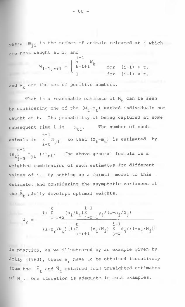
- 66 -

where is the number of animals released at j which

are next caught at i, andi-1tt W,

w .i-1,t+1 k=t+l1

for (i-1) > t. for (i-1) = t.

and W, are the set of positive numbers.

That is a reasonable estimate of M can be seen

by considering one of the (M -m ) marked individuals not

caught at t. Its probability of being captured at some

subsequent time i is mti* The number of sucht-1

animals is l m.. so that (M -m ) is estimated by i=0 3

t-1(s Z m.. )/m,.. The above general formula is atj = 0 J1 T1

weighted combination of such estimates for different

values of i. By setting up a formal model to this

estimate, and considering the asymptotic variances of

the M , Jolly develops optimal weights:

Wr

k i-11+ £ (n. /N. ) E 4> ./ (1-n ./N .)

i=r+2 1____ j=r+l 3______3 3k

(1-n /N )(1+E (n./N.)r r i-r+l 1 1

i_1 iZ <*>./(l-n./N .)> j_r J J J

In practice, as we illustrated by an example given by

Jolly (1963), these Wr have to be obtained iteratively

from the $ and N _ obtained from unweighted estimates

of M _. One iteration is adequate in most examples.

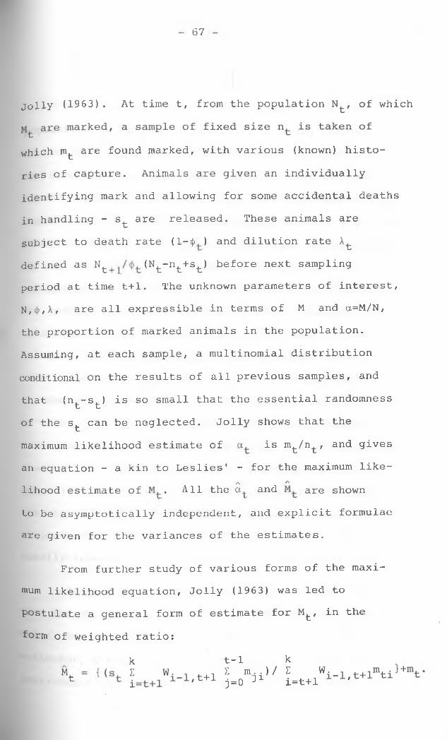
67

jolly (1963). At time t, from the population Nt, of which

which mfc are found marked, with various (known) histo­

ries of capture. Animals are given an individually

identifying mark and allowing for some accidental deaths

in handling - st are released. These animals are

subject to death rate (l-c|> ) and dilution rate At

defined as **t + (Nt-nt+st) before next sampling period at time t+1. The unknown parameters of interest,

N,<j),X, are all expressible in terms of M and a=M/N,

the proportion of marked animals in the population.

Assuming, at each sample, a multinomial distribution

conditional on the results of all previous samples, and

that (nt-st) is so small that the essential randomness

of the s_£ can be neglected. Jolly shows that the

maximum likelihood estimate of is m^/n^, and gives

an equation - a kin to Leslies' - for the maximum like-A Alihood estimate of . All the a_ and are shown

to be asymptotically independent, and explicit formulae

are given for the variances of the estimates.

From further study of various forms of the maxi­

mum likelihood equation, Jolly (1963) was led to

postulate a general form of estimate for M^, in the

form of weighted ratio:

Mtk t-1 k

I m . . )/ l Wj=0 -1 i=t+l

68

We now discuss the stochastic models. If the

population is subject to naturally occuring changes,

in the form of birth, death, migration, and growth,

any comprehensive theory must take into account the

natural variability between individuals in respect of

these changes. If not only the population but also the

observed samples are large in number, and interest lies

in the behaviour of an 'average' individual in the

population, this variability contributes negligibly to

the variability of the estimates of the behaviour of

this hypothetical animal. Every individual can then be

assumed to behave identically; a deterministic model,

such as we have considered in the previous sections,

is adequate. However in most practical studies it

is stretching the definition to assume large samples.

Since the stochastic models describing capture-recapture

studies have recently been shown by Jolly (1965) and

Seber (1965) not only to be less complicated to analyse

than the corresponding deterministic models, but also

to provide more valid results, these methods should

totally supersede their deterministic counterparts.

Although some earlier workers had pointed out

that the variance of an estimator from a deterministic

Model would underestimate the true variance of the

estimator, Moran (1952) was the first to discuss the

implications of deterministic and stochastic models in

- 69 -

this context. A truly deterministic model is virtually

unworkable in practice since, if the proportion <J> of

the population survive between sampling at time t and

t , not only <b N but also d> M - and the size of J o o o oany other survival class - is restrained to be an

integer. Thus an approximation has to be introduced

by assuming that all values such as ^0N0 can regarded

as integers. Under the assumption of multinomial, rather

than multi-hypergeometric, sampling, the probability

distribution, assuming integers, of the set of observed

recaptures remains a probability distribution if the

<t) N and so on are integers. This difference defines fo othe 'deterministic model' which can only be an approxi­

mation to what really happens. Moran points out that

Leslie and Chitty (1951) and Leslie (1952) use a 'semi-

probabilistic' model. In this, a fixed proportion <J>

of the population survives, but the Nq (|)o individuals

surviving are chosen at random without reference to

their markings. A fully probabilistic model assumes

that each individual independently has a probability

$ of survival, the number which survive being a random

variable binomially distributed with index Nq and

parameter <b . Moran does not attempt to analyse this oModel, being deterred by the difficulty that the sample

numbers n^ can not be prescribed in advance since there

is a non-zero probability that fewer than n^ animals

70

are alive at that time.

The way round this difficulty was noted first by

Hammersley (1953). The sampling scheme hitherto consi­

dered have all assumed that the sample on each occasion

is complete when a predetermined number of animals have

been captured. In practice, however, sampling usually

ceases through a decision of the experimenter determined

by the effort expended, and not the number of animals

caught. Each individual may be assumed to have the

same probability of capture, p^, during the ith sample

period, the size of that sample being thus binomially

distributed with index ISL . The p^ are parameters,

sometimes to be estimated from the data, sometimes

considered as known except for a single constant

of proportionality; the n^ are random variables. This

simple change of outlook, bringing theory more into

line with practice, circumvents the difficulties of

a stochastic approach. Unfortunately, as shown by

Dorrah (1959), Hammersley's subsequent analysis is

based on an incorrect model for the likelihood function.

Hammersley does consider the population to be of

two different classes, young and adult, with different

survival rates, the one growing into other during the

course of the experiment.

The distinction between the two models was first

71

brought out by Darroch (1958) in his analysis of a

closed population. The earlier model with fixed sample

size (Darroch's model B) "is likely to be appropriate

when the main limiting factor on the sample size is the

trouble involved in marking animals". The new model

(Darooch's model A) "when it is the difficulty in

catching them". The simplicity of the multinomial

distribution implied by the new model, rather than}

the mult ihypergeometric model, enables Darroch (1959)

to derive the maximum likelihood estimators for the

unknown parameters when either death or immigration,

but not both, are affecting the population. Seber

(1962) derived maximum likelihood estimates for a model

appropriate to commercial fisheries. A series of batches

of marked individuals are released, after each of which

-allowing time for redistribution of the marked animals-

a commercial catch is taken and this is immediately

followed by the release of more marked fish. Seber

shows that if only one release followed by a number of catches is made and no immigration or emigration is

assumed to occur, his model becomes a discrete equivalent

of Gulland's(1955) model for a coni Inouos fishery.

These methods of Darroch and Seber are special

cases of a general theory proposed independently by

dolly and Seber (1965). Since Jolly's model is slightly

more general than Seber's in that it allows for the

72

removal, either deliberately or by accident, of some of

the animals caught in any sample, it will be discussed

here. A part from this modification, the estimates

obtained by Jolly and Seber are identical.

At time t^, a population of individuals,

of which are marked by a mark which identifies the last

occasion on which they were caught, is sampled in

such a way that each individual in the population has

probability p^ of being captured. This results in a

sample of n^ individuals, nr of which are marked. After

this sample each of the n^ has probability of being

marked and released again, individuals being released

into the population. Between t. and t^+1 the population

of (N.-n. + s.) individuals is altered by the effect of 1 1 1

death (or emigration) each individual independently

having a probability (1—4> ) of leaving the population;

and also by immigration of a number of new individuals,

Bi of which are alive in the population at time ti+l*Of these parameters Nq ,B^, p^,4>^, are unconditional.

The others N. and M. are conditional on events prior to 1 1t^. This means that the general probability distribution

of Nji , Mji , mj ± , U±, ui,si (where Mj± and ± are the numbers in the population and sample at time t^

which were last caught at t^ and U^, u^ those that have

never been caught), conditional on the fixed parameters

Nq, B^, p., <j) nif is not identical to the likelihood

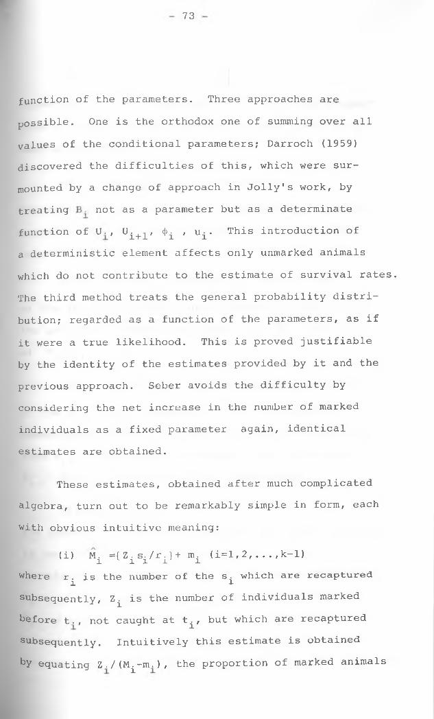
73

function of the parameters. Three approaches are

possible. One is the orthodox one of summing over all

values of the conditional parameters; Darroch (1959)

discovered the difficulties of this, which were sur­

mounted by a change of approach in Jolly's work, by

treating not as a parameter but as a determinate

function of lh, U^+1, <J> , u^. This introduction of

a deterministic element affects only unmarked animals

which do not contribute to the estimate of survival rates.

The third method treats the general probability distri­

bution; regarded as a function of the parameters, as if

it were a true likelihood. This is proved justifiable

by the identity of the estimates provided by it and the

previous approach. Seber avoids the difficulty by

considering the net increase in the number of marked

individuals as a fixed parameter again, identical

estimates are obtained.

These estimates, obtained after much complicated

algebra, turn out to be remarkably simple in form, each

with obvious intuitive meaning:

(i) M. ={Z.s./r.}+ m. (i=l,2,...,k-1) l 1 l l iJ rwhere r. is the number of the s. which are recaptured l isubsequently, Z^ is the number of individuals marked before t., not caught at t^, but which are recaptured subsequently. Intuitively this estimate is obtained by equating Z./(M^-nr), the proportion of marked animals

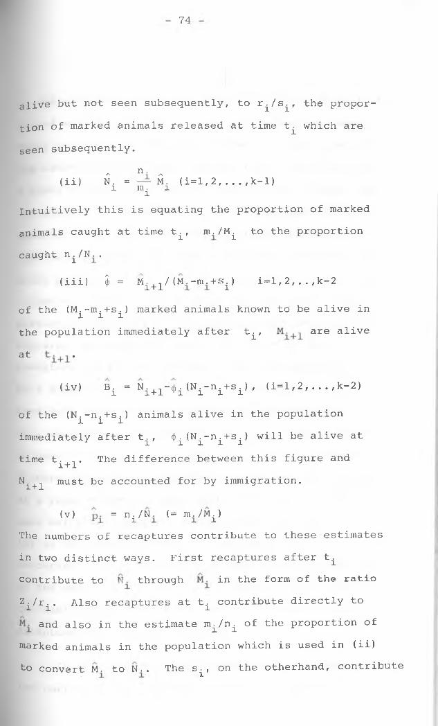
74

alive but not seen subsequently, to r^/s^, the propor­

tion of marked animals released at time t^ which are

seen subsequently.

- n. „(ii) Ni = HT Mi (i=l/2,...,k-l)

iIntuitively this is equating the proportion of marked

animals caught at time t^, itk/M^ to the proportion

caught n^/IT.

(iii) $ = Mi+i/(NL-nr+s^ i=l, 2, . . ,k-2

of the (M^-m^+s^) marked animals known to be alive in

the population immediately after t^, are alive

at H + r

(iv) Bi = Ni+1-(()i (Ni"ni+si) , (i=l, 2,--,k-2)

of the (N.-n.+s.) animals alive in the populationi l limmediately after t^, <j> (N^-n^+s^) will be alive at

time t^+ . The difference between this figure and

Ni+1 must be accounted for by immigration.

(v) = n^lL (= nr/Mi)The numbers of recaptures contribute to these estimates

in two distinct ways. First recaptures after t^

contribute to through in the form of the ratio

Z^/r^. Also recaptures at t^ contribute directly to

and also in the estimate m^/n^ of the proportion of

marked animals in the population which is used in (ii)

to convert M. to N.. The s. , on the otherhand, contribute

75

to the estimates only in the form of creating a pool of

marked animals from which later samples may be taken.

There is no direct connection between and n^,nK in

the estimation procedure. Seber's (1965) estimates for

a model in which no losses on capture are allowed, are

identical with those given if s^ is put equal to n^.

Moreover Jolly shows that Seber's (1962) estimates can

also be expressed by the above relations, because, as

Jolly points out, the only relevant information is the

occass:ion on which an individual was last seen. Its

history of capture prior to the last previous sighting

contains no information about its chance of death or

recapture after that sighting. The information provided

by a single individual caught at times t ., t ., t , is1 J Kprecisely the same as if one individual released at t.

were recaptured (and removed) at t^, a second individual

released at t^ and recaptured at t^. Thus a commercial

fishery with single recapture yields the same estimates

as a research project with multiple recapture. The

name multiple recapture is thus irrelevant, at least as

far as the estimation of the population parameters is

concerned. If interests lie in testing the assumptions

of the model, particularly with regard to the equal

catchability of individuals, then information on multiple

recaptures does become valuable.

It is interesting to compare these estimates with

the corresponding estimates obtained on the basis of

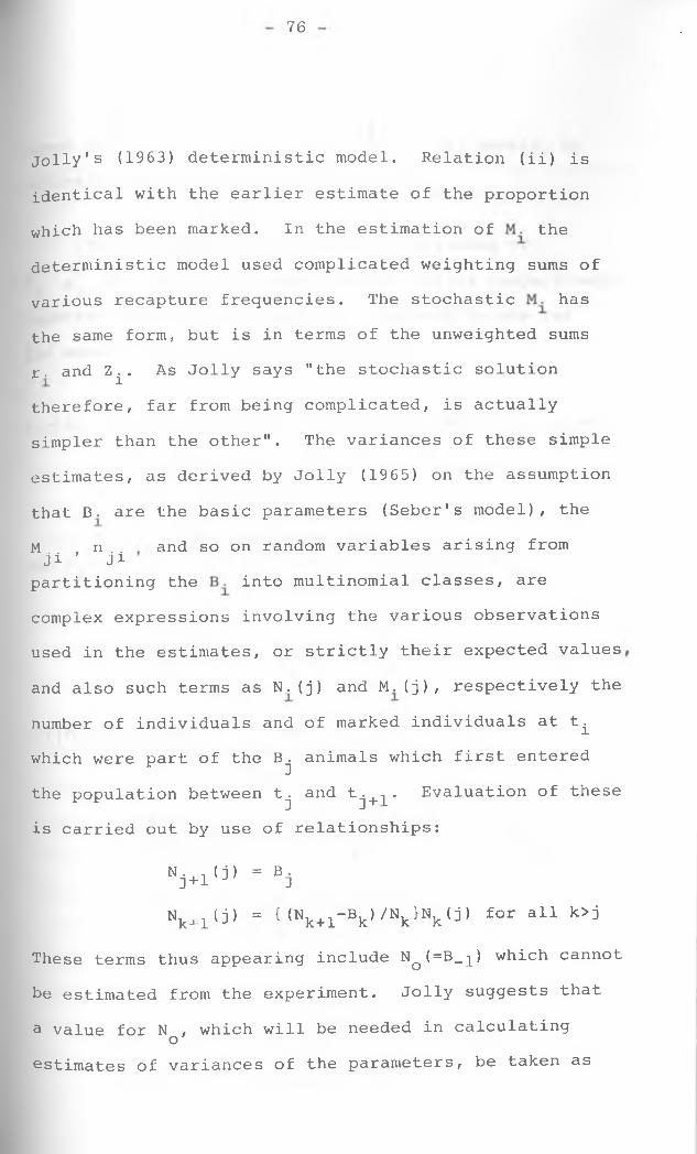
76

jolly's (1963) deterministic model. Relation (ii) is

identical with the earlier estimate of the proportion

which has been marked. In the estimation of the

deterministic model used complicated weighting sums of

various recapture frequencies. The stochastic has

the same form, but is in terms of the unweighted sums

r. and Z^. As Jolly says "the stochastic solution

therefore, far from being complicated, is actually

simpler than the other". The variances of these simple

estimates, as derived by Jolly (1965) on the assumption

that B. are the basic parameters (Seber's model), the

M n and so on random variables arising fromji ’ jipartitioning the into multinomial classes, are

complex expressions involving the various observations

used in the estimates, or strictly their expected values

and also such terms as ISL(j) and JVL(j), respectively the

number of individuals and of marked individuals at t^

which were part of the B^ animals which first entered

the population between t^ and tj + -. Evaluation of these

is carried out by use of relationships:

Nj + 1(j) = Bj

NkJi (j) = { (Nk+l"Bk)/Nk }Nk (j) for a11 k>j

These terms thus appearing include N^(=B_^) which cannot

be estimated from the experiment. Jolly suggests that

a value for N , which will be needed in calculating oestimates of variances of the parameters, be taken as

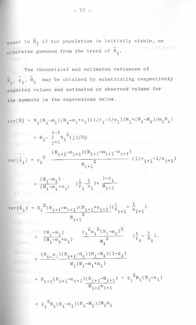
77

equal to if the population is initially stable, or✓N

otherwise guessed from the trend of INh.

The theoretical and estimated variances of

J., EL may be obtained by substituting respectively

expected values and estimated or observed values for

the symbols in the expressions below.

var[N] = Ni(Ni-mi)[Mi-mi+si)(l/ri-l/si)/Mi+(N1-Mi)/miNi]

i_1 2+ N.- I N.Z(j)/Bjj = l

(Mi + l-mi+l)(Mi+l"rni+l'Si + l)var[$. ] = -------------2 0 / ri+1_1/si+x

Mi+1

,1 1 u H i+ (M.-m^s.) S;L M.+1

var [Bi] = B.2(M. + 1-m 1+1)(M.+1+s.+1)( ^ - f . ^ )

* W

( M . -m. )v l l2 2 / ]\J m X2

l l v l iM.l

2(Mi-mi+si)

(Ni_njL)(Ni + 1-Bi))Ni-Mi)(l-»i)

Mi^Mi-mi+Si)

(i - i ).ri si

+ Ni+l(Ni+l-ni+X)i1W ^ i ± l ) + n 2Ni(Ni-ni>

78

Similar expressions for the covariances of the estimates

may be found in Jolly. The termsi-l 2

N. t N. (j)/B.1 j = l 3

in var [ N i ] and i+1 in

var[(|) ] are contributions to the variance from the

conditional nature of and <Jk .

Jolly's initial formulation of the problem is even

more general than has been described here. The joint

probability distribution from which the estimates are

derived, is stated from a heterogeneous population

that is, for a population composed of different classes

(for example, sexes) between which there is no migration.

If all parameters are different for each class, each

class may be analysed as a homogenous population. But

if some parameters, perhaps survival rate or probability

of capture, are common to different classes, more

complex estimation equations would have to be constructed,

and solved by iteration. Jolly (1965) also analyses

the restricted cases of "death, no immigration" and

"immigration, no death", showing that, when s^=n^, bis

estimates and their variances are identical with those

given earlier by Darroch (1959). These restricted

models should not be used, now that a simple analysis

of the general model is available (Cormack (1968)) .

In common with earlier, simpler models, these

- 7Q _

likelihood estimates can be considerably biased if the

numbers of recaptures are small. Seber (1962, 1965)

suggests modifications , similar in form to those of

both Bailey and Chapman which lead to almost unbiased

estimates with a negligible loss of efficiency. For

the case of no losses on capture, n^=s^, the modified

estimate of is

M* = Z .(S.+1)/(r.+1) + (m.+l);l i l l l

The estimates N*, cj)?, B?, p* being the same functions

of M* as N. , d>. , B. , p. are of M. . A precisely similar i i Yi l r i i

modification, adding unity to each observation except

Z is shown by Seber (1962) to yield almost unbiased

estimates for the single recapture census.

Alternative description of the properties of

dilution and survival are introduced by Jolly (1963)

and Seber (1965), respectively. Jolly defines a

dilution rate A^ as the ratio of the population size

at t^+ to the survivors at that time of the population

st t^. He gives an expression of A^ as:

Xf = [*i (Ni-ni+si)+Bi]/4)i (Ni-ni+si)

'the estimate of A^ is merely the corresponding function

°f other estimates. This representation has the advantage

that A. is estimable although B^_^ is not. Seber (1965)

considers an instantaneous death rate during the

80

period ( , t^+1), defined by the relation

cj) = e ^i^i+l fci . Again its estimate is the corres­

ponding function of the estimate of <Jk .

One further extension of this model was suggested

by Darroch (1958, 1959) but not by the later authors,

except Seber (1965) makes use of the idea in constructing

at test of the assumptions. In many fields of study

a measure of the effort, f^, put into the sampling at t^,

is available. This usually takes the form of the number

of man-hours expended, or in commercial catches, the

total number of gear used. If f^ are known, and the

catchability (q) of all individuals remains constant

throughout the experiment, the p^ are known functions

of a single unknown parameter q. Most earlier authors

have assumed that p^ = qf^. Darroch (1958) makes the

assumption that the probability of any individual being

caught when subjected to df units of effort is qdf,

which leads to the model p^= 1-e ^ i . As manageable

approximation to this, Darroch uses p^=qf l-qf^/2). For the

models assuming death or immigration but not both, Darroch

derives an approximate maximum likelihood estimator for

and modifies it in the usual way to provide an almost

unbiased estimator. The estimator p^ may be replaced by

^ i (1—qf^/2) f and this used in the subsequent estimation

°f the other population parameters. Darroch gives a

able showing the increase of information about provided

81

by this knowledge of effort.

The only other model to have received a fully

stochastic treatment in these terms was proposed by

Cormack (1964). This refers to the situation in which

recapture information is available on marked individuals

only, random sampling of the whole population being

impossible. Estimates were obtained for the mortality

of the marked population. For these estimates to be

applicable to the whole population some assumptions of

the representative character of the marked animal is

required. In general no estimate of the population size

is possible from such data, although Jolly (1965) points

out that, "whether or not the survival rates are the

same for the two populations, provided they have the

same probability of being captured in a sample", an

estimate of is possible. If, however, as in the

data from Dunnet, Anderson and Cormack (1963) discussed

by Cormack (1964), sampling of the marked and unmarked

individuals are total.Ly separate, the proviso in Jolly's

statement will be impossible to fulfil. Similar data may also be obtained in commercial studies, n^ not being recorded although nr is. Again cannot be estimated

and the survival estimates cf> apply strictly only to

the marked population. This situation fits easily

into Jolly's frame work within which and n^ need

not be composed of the same individuals, and Jolly has

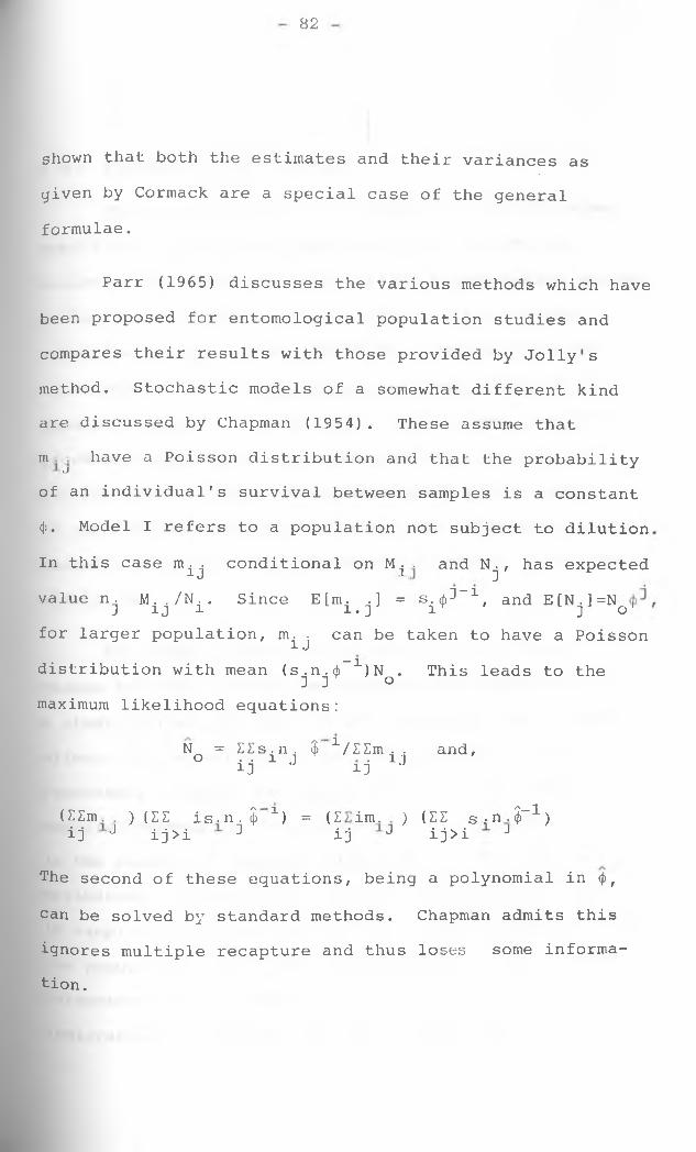
82

shown that both the estimates and their variances as

given by Cormack are a special case of the general

formulae.

Parr (1965) discusses the various methods which have

been proposed for entomological population studies and

compares their results with those provided by Jolly's

method. Stochastic models of a somewhat different kind

are discussed by Chapman (1954). These assume that

in have a Poisson distribution and that the probabilitytJof an individual's survival between samples is a constant

<J>. Model I refers to a population not subject to dilution

In this case m ^ conditional on M_j • and N^, has expected

value n. M../N.. Since E[m. .] = s . ^ " 1, and E[N.]=NJ ij i l.] l K ' 1 j J o 'for larger population, m. . can be taken to have a Poisson1 Jdistribution with mean (s^n^ (J)”1) Nq . This leads to the

maximum likelihood equations:

N = ZZs.n. $ 1 /1Zm . . and, o . . 1 j r . 11 'ij ° ij J

a i m ) a z is.n. $ 1) = (Z im. ) (IZ s.n.J'1 )ij J ij >i J ij J ij >i J

The second of these equations, being a polynomial in (p,

can be solved by standard methods. Chapman admits this

ignores multiple recapture and thus loses some informa­

tion.

83

2.2 STATEMENT OF THE PROBLEM.

The estimation of total population size of animal

populations is of great importance in a variety of

biological problems which may relate to population growth,

ecological adaptation, genetic constitution, natural

selection and evolution, and so on. Obvious practical

consequences are the maintenance of human supplies of

food and control of insect pests. For human communities

procedures employing fixed sampling units are available,

but for mobile populations other methods must be used.

Of the methods available for obtaining information about

animal populations, capture-recapture method is the most

widely used.

Any animal population is subject to continual

change by birth, death, immigration and emigration. In

a study carried out over a short period of time, these

effects may be negligible and the experimenter may

reasonably consider the population as closed. More usually,

temporal changes in the population are of primary interest;

is the population growing, stationary or heading for

extinction? A study over a longer time-scale is required.

If sampling continues over an appreciable period of time,

the population can no Longer be considered closed. Other

parameters of recruitment and mortality (and possibly

immigration &nd emigration) must be included in the model.

84

A detailed study of such parameters as mortality rates,

survival rates and total population size, provide the

information required to generate enough scientific

guidelines and advice for rational exploitation,

management and utilization of renewable resources.

Hence the need to study them.

Estimation of population size is important in the

following areas: the exploitation of fresh water fish

for food, the removal of insect pests from crops, the

control of Tse-Tse flies, the destruction of verminous

small mammals by poisoning, the control of an out break

of an desease, and so on.

The aim of this dissertation is to study capture-

recapture models for estimation of population size. We

shall also give an application of these models to the

real-life data. More specific objectives are listed below.

1) To review some capture-recapture models used in the

estimation of population size.

2) To apply the selected model(s) to the real life

data.

3) To study the departures from the underlying

assumptions

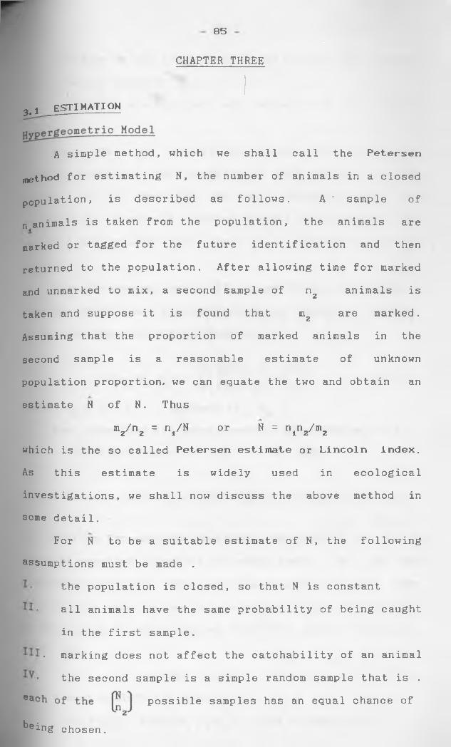
r85

CHAPTER THREE

3.1 ESTIMATION

A simple method, which we shall call the Petersen

j ethod for estimating N, the number of animals in a closed

n animals is taken from the population, the animals are

marked or tagged for the future identification and then

returned to the population. After allowing time for marked

Assuming that the proportion of marked animals in the

second sample is a reasonable estimate of unknown

population proportion, we can equate the two and obtain an

estimate N of N. Thus

which is the so called Petersen estimate or Lincoln index.

As this estimate is widely used in ecological

investigations, we shall now discuss the above method in

some detail.

For N to be a suitable estimate of N, the following

assumptions must be made .

the population is closed, so that N is constant

all animals have the same probability of being caught

in the first sample.

• marking does not affect the catchability of an animal

• the second sample is a simple random sample that is .

population, is described as follows. A ‘ sample of

and unmarked to mix, a second sample of n2 animals is

taken and suppose it is found that mz are marked.

m2/nz = ni/N or N = n, n2/ m2

possible samples has an equal chance of

^®ing chosen.

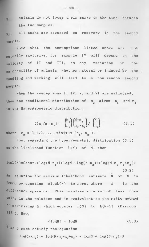
86

animals do not loose their marks in the time between the two samples.

yj all marks are reported on recovery in the second

sample •Note that the assumptions listed above are not

nutually exclusive, for example IV will depend on thevalidity of II and III, as any variation in thecatchability of animals, whether natural or induced by thehandling and marking will lead to a non-random secondsample.

When the assumptions I, IV, V, and VI are satisfied,then the conditional distribution of m given n 2 1 and n 2

is the Hypergeometric distribution.

f ( W n 2) = (n‘] £2 2 - d ' ■ C ) (3. 1 )

where mz = 0 ,1 ,2 ,..., minimum (n ° 2 )•Now, regarding the hypergeometric distribution (3.1)

as the likelihood function L(N) of N, then

logL(N)=Const.+log(N-ni)!+logN!+log(N-nz)!+log(N-ni-n2 +m2)!(3.2)

An equation for maximum likelihood estimate N of N is found by equating AlogL(N) to zero, where A is the diffe rence operator. This involves an error of less than unity in the solution and is equivalent to the ratio method °f maximizing L, which equates L(N) to L(N-l) (Darroch, 1958) . Now,

AlogN! = logN (3.3)Thus N must satisfy the equation

log(N-n±) - log(N-ni~n2+m2) - logN + log(N-n2) = 0

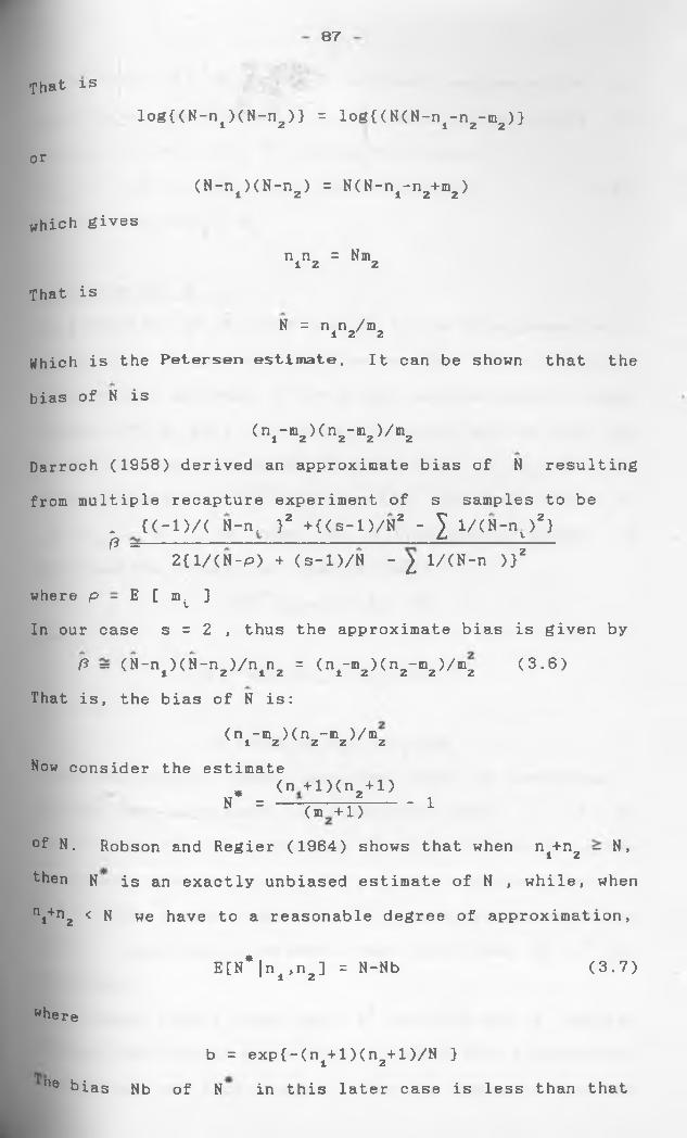
87

That islog{(N-ni)(N-n2)} = log{(N(N-ni-n2~m2)}

or

(N-ni)(N-n2) = H(H-nr n2+B2)

n n = Nm 12 2

which gives

That isN = nin2/m2

Which is the Petersen estimate. It can be shown that the bias of N is

(nr m2 )(n2-m2 )/m2

Darroch (1958) derived an approximate bias of N resultingfrom multiple recapture experiment of s samples to be

. {<-l>/( N-n. } 2 +{<s-l)/N2 - 7 1/(N-n )2}ft =-------------------------------^------- i---

2{1/(N-P) + (s-l)/N - 2 l/(N-n ) } 2

where p - E [ m. ]LIn our case s = 2 , thus the approximate bias is given by

ft = (N-ni)(N-n2 )/nin2 = (ni-m2 )(n2-m2 )/m2

That is, the bias of N is:(3.6)

(nl-m2)(n2-in2)/ni2

Now consider the estimate. (n + 1 )(n + 1 )

N = — —7 —=4--------1(m +1)°t N. Robson and Regier (1964) shows that when n 1 + n 2 - N, then N is an exactly unbiased estimate of N , while, when nt+n2 < N we have to a reasonable degree of approximation,

E[N*|n ,n ] = N-Nb 1 1 2 (3.7)

whereb = exp{-(ni+l)(n2+l)/N }

ne bias Nb of N in this later case is less than that

is almost an unbiased estimate of N and0f N . Thus N*hence it is more preferable to N as an estimate of N. It is easy to check that N is the solution of

(N - n±)(N - n2) = (N + 1)(N - r) (3.8)

where, r “ ni + n2 ~ m2 '

P r o p e r t i e s o f N.

The properties of N with respect to the hypergeometric distribution have been fully discussed by Chapman (1951). He shows that although N is a best asymptotically normalestimate of N as N ----- >oo, it is biased and the bias canbe small for small samples. However, when n±+ n2 >N , his modified estimate, N is exactly unbiased, while if ni + n2 < N , we have, to a reasonable degree of approximation (Robson and Regier(1964))

E[N*|n1,n23 = N - Nbwhere,

Def iningb = exP{-(n1+l)(n2+l)/N }

P = E{m2/n±,n2} = n ^ / NRobson and Regier (1964) recorded that in designing a Petersen type experiment it is essential that p >4, so that b is small. They also say if mz > 7 in a givene*periment, then we can be 95 per cent confident that^ >4 . This implies that for 7 or more recaptures we can be 9 5 per cent confident that the bias of N* isnegligible.

Chapman (1951) shows that N not only has a smaller xPected mean square error than N for values encountered lri Practice, but also appears close to being a minimum

variance unt,iase< estimate over the range of parameter values for which it is almost unbiased. Using what isessentially a Poisson approximation to the hypergeometric model (3.1), he shows that the variance of N* isapproximately given by

V[N*|ni,nz] S N(/u'1+2/j'2+6p '3) (3.9)

* 4tAn estimate V say, of the variance of N is obtained*by simply replacing N by N in (3.9). However, an

approximate unbiased estimate has been given by Seber (1970) and Wittes (1972), namely

V[N*|ni,nz] = (ni+l)(n2+l)(ni-m2 )(n2-m2 )/(m2+l)(m2+2).

2which has a positive proportional bias of order ^ exp-AJ It*can be shown that V is exactly unbiased when n±+nz>N .

4tThe co-efficient of variation of N is approximatelygiven by

C[N*] = 1/V£

and if a rough estimate of N is available before theexperiment, n± and nz can be chosen before hand to give adesirable value of C. We note that an estimate of C isobtained by replacing v by mz , giving C = 1/Vmz . Thismeans that the "accuracy” of N is almost solely dependent°o the number of recaptures in .2

hailey’s Binomial Model.Assume that n2 is sufficiently small compared with

" for us to be able to ignore the complications of sampling without replacement. The large sample theory of ft3cimum likelihood approach will be appropriate if we

90

envisage n , nz and N all tending to infinity while keeping constant ratios to each other. Then using the binomial approximation to hypergeometric distribution (3 .1 ), the likelihood function becomes

f ( V W * E a) ( r ] * t1- r )

< n -m > 2 2

(3.10)

therefore

L= log{f(m /n ,n )}= constant+(n -m )log(N-n )- n logNX £ b X

(3.11)Differentiating (3.11) with respect to N gives

6 L<5N (n2-m2 )/(N- n±) - n2/N (3.12)

Hence, the maximum likelihood estimate of N satisfies

(n2 - m2) /(N - n±) = n/N

that isN(n2 - m2) = n2(N-n±)

or ,Nm = n n 2 12

Therefore

N = n±n2/m2 (3.13)which is Petersen’s estimate. Expanding N as a taylor series in powers of t(=m2~m), where m=E[mz], and taking the expectation of both sides we have

E[N] = N{ 1 + (N-ni)/nin2 + o(m'2)}= N{ 1 + 1/m + o(m~2) } (3.14)

Thus, clearly, the bias of N is approximately Nm-1 .Now consider the estimate

N ' = n4(n2 + l)/(m2 + 1 )

- 91 -

Then,

E[N']n , . .-2 n1<n2 + 1>X o (B2+1>

<n -m > 2 2

)

<n -m > 2 2

Thus the bias of N ' is approximately Nexp(-m) which is

quite small even for moderate m. Thus N' may be preferreda

to N as an estimate of N.

To get the variance of N, we differentiate equation

(3.12) with respect to N and taking expectations provides

the required information in the case of a single sample.

Thus:

In = -E [32L / a n 2 ) = nin2/{N2(N-nl) (3.16)

Using N = n n /m 1 2 2Var[ N ] = C = n2 n2(nl-»2)/m2

We note that var[ N ] is infinite if we admit the value

m2 = 0. On the other hand, this value will occur so rarely

in large samples for which m = E[ ra2] is not small, that

w© can choose to omit it.

A satisfactory expression for the variance of N ' is

somewhat more difficult to find. However using the

'method described in chapter one, we can derive the

Asymptotic series

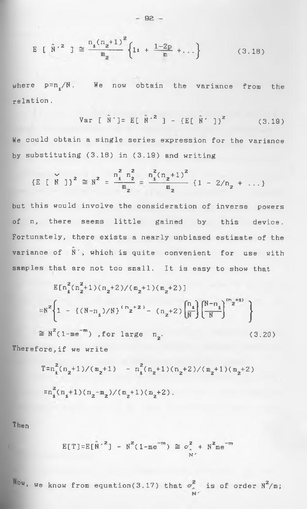
92

. 2 n (n + 1 )E [ N ' ] = — — ----

{Il + H r +- - } <3 -18>

where p=ni/N. We now obtain the variance from the relation.

Var [ N ' ] = E [ N'2 ] - {E[ N ' ]}2 (3.19)

We could obtain a single series expression for the varianceby substituting (3.18) in (3.19) and writing

2 2 2, „ n2 ^ 2 2 ni nz n (n + 1 )(E [ N ] } 2 = N 2 = l---- (1 - 2/nz + ...}

2 2

but this would involve the consideration of inverse powers of n, there seems little gained by this device.Fortunately, there exists a nearly unbiased estimate of the variance of N', which is quite convenient for use with samples that are not too small. It is easy to show that

2 , 2E[ni(n2+l)(n2+2)/(m2+l)(m2+2)]

,■ {1 - {(N-nl)/N}‘,V 2>- (nz+2)[ N «v ^

S F ? ) }= Nz(l-me m ) ,for large n2- (3.20)

Ther efore,if we write

T=n2 (n2+l)/(m2+l) - n2 (n2+l )<nz+2)/(m2+l)(m2+2 )

=n2( 1 )(n2-m2)/ ( m2+ 1 ) < mz + 2 ) .

Then

E[T]=E[N'2] - Nz( 1-me "’) ^ o-f + Nzne mN '

0w> we know from equat ion( 3.17) that is of order Nz/m;

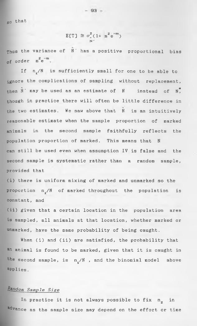
so that

E[T] 3 a?(1+ nze m )N '

Thus the variance of N' has a positive proportional bias, 2 -m0f order m eIf n4/N is sufficiently small for one to be able to

ignore the complications of sampling without replacement,* 4|tthen N' may be used as an estimate of N instead of N,

though in practice there will often be little difference in the two estimates. We saw above that N is an intuitively reasonable estimate when the sample proportion of marked animals in the second sample faithfully reflects the population proportion of marked. This means that N can still be used even when assumption IV is false and the second sample is systematic rather than a random sample, provided that(i) there is uniform mixing of marked and unmarked so the proportion n^N of marked throughout the population is constant, and(ii) given that a certain location in the population area is sampled, all animals at that location, whether marked or unmarked, have the same probability of being caught.

When (i) and (ii) are satisfied, the probability that an animal is found to be marked, given that it is caught in the second sample, is n^N , and the binomial model above aPPlies.

Qzndoni Sample Si ze

In practice it is not always possible to fix n2 in Advance as the sample size may depend on the effort or time

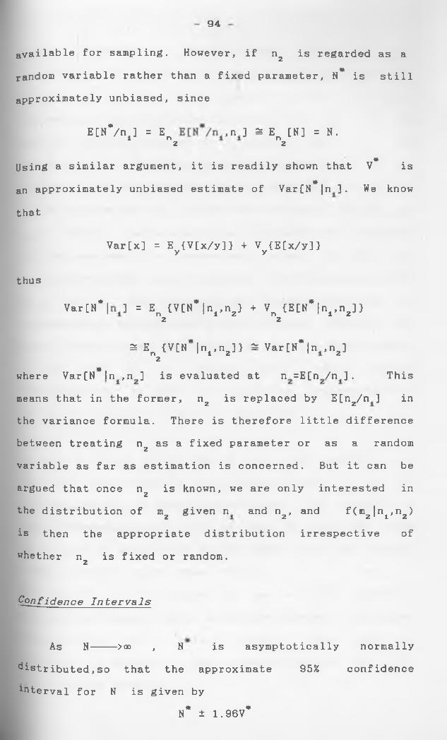
94

available for sampling. However, if n2 is regarded as a*random variable rather than a fixed parameter, N is still

approximately unbiased, since

E[N*/nt] = En ,n ] £ En [N] = N .2 2

*Using a similar argument, it is readily shown that V is*an approximately unbiased estimate of Var[N |n ] . We know

that

Var[x] = Ey{V[x/y]} + Vy{E[x/y]}

thus

Var[N* | ] = En {V[N* I n ^ } + Vn {E[N* | nA, n2] }2 2

2= En {V[H*|n1 ,n2]} 2= Var[N*|n ,n2]2*where Var[N In ,n ] is evaluated at n =E[n /n ]. This

means that in the former, n2 is replaced by E[n2/n ] inthe variance formula. There is therefore little differencebetween treating n2 as a fixed parameter or as a randomvariable as far as estimation is concerned. But it can beargued that once n2 is known, we are only interested inthe distribution of m2 given n and n2, and f(m2 |ni,n2)is then the appropriate distribution irrespective ofwhether n is fixed or random.

2

Confidence I n t e r v a l s

As N---->oo , N is asymptotically normallydistributed,so that the approximate 95% confidenceinterval for N is given by

* *N ± 1.96V

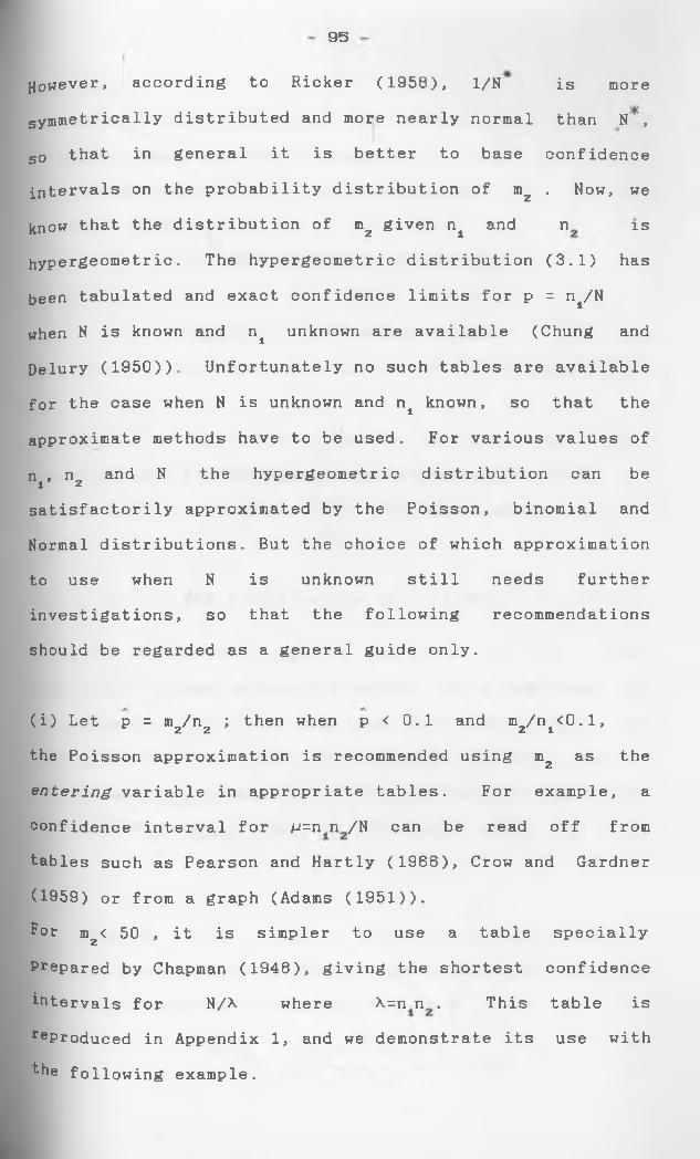
93

However, according to Ricker (1958), 1/N is moresymmetrically distributed and more nearly normal than N , s 0 that in general it is better to base confidence intervals on the probability distribution of mz . Now, weknow that the distribution of mz given n± and n. is

hypergeometric. The hypergeometric distribution (3.1) has

been tabulated and exact confidence limits for p = ^/N

when N is known and n± unknown are available (Chung and

Delury (1950)). Unfortunately no such tables are available

for the case when N is unknown and n± known, so that the

approximate methods have to be used. For various values of

n , n and N the hypergeometric distribution can be1 2satisfactorily approximated by the Poisson, binomial and

Normal distributions. But the choice of which approximation

to use when N is unknown still needs further

investigations, so that the following recommendations

should be regarded as a general guide only.

(i) Let p = m2/n2 ; then when p < 0.1 and m2/ni<0.1,

the Poisson approximation is recommended using m2 as the

e n t e r i n g variable in appropriate tables. For example, a

confidence interval for V = n n / H can be read off from

tables such as Pearson and Hartly (1966), Crow and Gardner

(1959) or from a graph (Adams (1951)).

Per m2< 50 , it is simpler to use a table specially

Prepared by Chapman (1948), giving the shortest confidence

intervals for N/X where X=n n . This table is

reProduced in Appendix 1, and we demonstrate its use with

the following example.

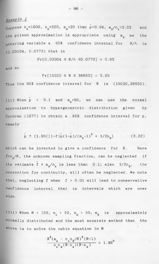
96

pvajnple 1

SupPose n1=100°> nz=500, mz = 20 then p=0.04, m2/ni=0.02 and the poison approximation is appropriate using mz as the

entering variable a 95% confidence internal for N/X is

(0.03004, 0.0773) that is

Pr[0.03004 < N/X <0.0773] = 0.95

and soPr[15020 < N < 38650] = 0.95

Thus the 95% confidence interval for N is (15020,38650).

(ii) When p < 0.1 and mz>50, we can use the normal

approximation to hypergeometric distribution given by

Cochran (1977) to obtain a 95% confidence interval for p,

namely

P ± {1.96{[l-f)p(l-p)/(m2-l)z + l/2nz} (3.22)

which can be inverted to give a confidence for N. Here

f=nz/N, the unknown sampling fraction, can be neglected if

its estimate f = m /n is less than 0.1; also l/2n . the2 1 2

correction for continuity, will often be neglected. We note

that, neglecting f when f > 0.01 will lead to conservative

confidence interval that is intervals which are over wide. (iii)

(iii) When N > 150, n± > 50, n2 > 50, m2 is approximately

normally distributed and the most accurate method than the

above is to solve the cubic equation in N

N2(m - n n /N)2(N-1)____f____ 1 __________ - in1n2(N-nl)(N-n2 ) “

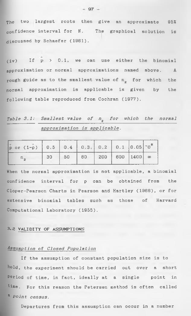
97

The two largest roots then give an approximate 95%

confidence interval for N. The graphical solution is

discussed by Schaefer (1961).

(iv) If p > 0.1, we can use either the binomial

approximation or normal approximations named above. A

rough guide as to the smallest value of n2 for which the

normal approximation is applicable is given by the

following table reproduced from Cochran (1977).

T a b le 3 . 1 : S m a l l e s t v a lu e o f n z f o r w h ic h t h e n o r m a l

a p p r o x im a t io n i s a p p l i c a b l e .

p or (1-p) 0.5 0.4 COo 0.2 0.1 0.05 ~0*

"2 30 50 80 200 600 1400 CD

When the normal approximation is not applicable, a binomial

confidence interval for p can be obtained from the

Cloper-Pearson Charts in Pearson and Hartley (1966), or for

extensive binomial tables such as those of Harvard

Computational Laboratory (1955).

3.2 VALIDITY OF ASSUMPTIONS

A s s u m p t io n of C lo s e d P o p u l a t i o n

If the assumption of constant population size is to

hold, the experiment should be carried out over a short

Period of time, in fact, ideally at a single point in

time. For this reason the Petersen method is often called

a P o i n t c e n s u s .

Departures from this assumption can occur in a number

of ways and we now discuss these in detail.

Accidental deaths

If there are d accidental deaths through the process

of catching and marking the first sample, the general

theory in section 3.1, remains unchanged provided that n

now refers to the number returned alive to the population,aN and N are estimates of N-d.

N a t u r a l M o r t a l i t y

Suppose that mortality is taking place in the time

between the two samples, and let N be the size of the

population when the first sample is released. When the

assumptions IV,V and VI of section 3.1, are true and the

only departure from I is due to mortality, the

hypergeometric model (3.1) still holds, provided the

mortality process is such that the deaths constitute a

simple random sample of known size. This follows from the

fact that the survivors will also constitute a simple

random sample from which the second sample is a random

sub-sample. Since a random sub-sample of a random sample

is itself a random sample, the second sample will still

represent a simple random sample from the original

Populat ion .

When deaths do not constitute a simple random sample,

the Petersen estimate can still be used provided the marked

and unmarked have the same average probability of surviving

UP till the time of the second sample. This can be seen

lrituitively from the equation.

- 98 -

99

(3.23)

We note that mortality is often selective with regard to

sample is a simple random sample, the more "vulnerable"

individuals will be proportionately represented in both

marked and unmarked populations, thus ensuring that marked

and unmarked have the same survival probabilities.

To examine the effect of variable mortality in the

marked proportion, suppose that there are various

subcategories in the population with numbers x, y,...., w

where N = x + y +....+W. For the marked members of these

categories, let 4> ,<P ,...,<£ be the respective survivalx y vprobabilities and let p 2x, P2y, • • • • >P2v the

probabilities of recapture in the second sample. Then

using suffix x to denote membership of category X, we

the size or age of the animal. However, if the first

have

(3.24)

and we can test the hypothesis

. - <P pv 2 v

using a standard chi-squared test based on the following

contingency table:

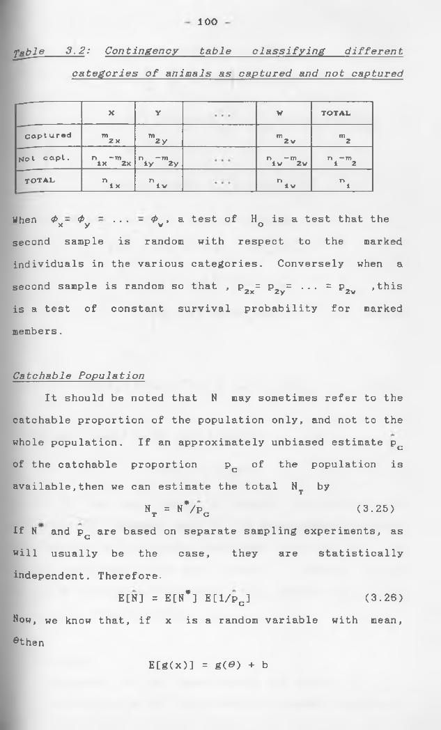
100

fable 3 . 2 : C o n t i n g e n c y table c l a s s i f y i n g different

c a t e g o r i e s o f a n i m a l s as c a p t u r e d and not captured

X Y W TOTAL

Captu red m m m m2 x 2 y 2 v 2Not capt. n -m n — m n -m n — mlx 2x ly 2y lv 2 v 1 2

t o t a l n n n n1 X 1 w 1 V 1

When <p - (p - ... - <p t a test of H is a test that thex y v Osecond sample is random with respect to the marked

individuals in the various categories. Conversely when a

second sample is random so that , p = p = ... = P,2x 2y 2v , this

is a test of constant survival probability for marked

members.

Catchable P o p u l a t i o n

It should be noted that N may sometimes refer to the

catchable proportion of the population only, and not to the

whole population. If an approximately unbiased estimate pCof the catchable proportion p of the population isCavailable,then we can estimate the total Nt by

Nt = N*7pc (3.25)If N and p are based on separate sampling experiments, asCwill usually be the case, they are statistically

independent. Therefore.

E[N] = E[H*] E[l/pc] (3.26)

Now, we know that, if x is a random variable with mean,

®then

E[g(x)] = g(0) + b

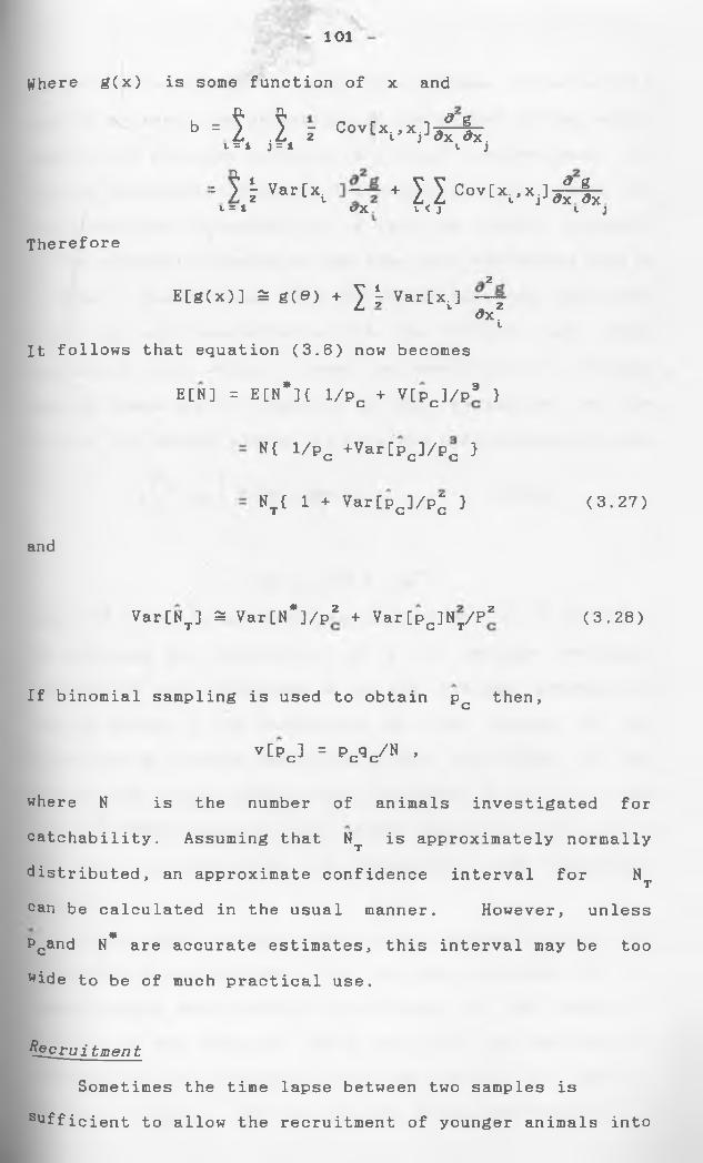
101

Where g(x) is some function of x and

b = 1 1 I Cov[xt'xj]3f-fc.I = 1 J = 1 V J

= 1 ) Var[xi + I I Cov[xi’xj]3f-fct = 1 wX t < J V JTherefore

2E[g(x)] ^ g(0) + 7 \ Var[x. ]

^ 1 <Jx2iIt follows that equation (3.6) now becomes

E[N] = E[H*]{ l/pc + V[pc]/pa }

N{ 1/p c +Var[pc]/pc }

Nt{ 1 + Var[pc]/p^ ) (3.27)

and

Var[Nx] 3 Var[N*]/P* + Var[pc]Nx/P* (3.28)

If binomial sampling is used to obtain p then,c

v[pc] = Pcqc/N ,

where N is the number of animals investigated for

catchability. Assuming that Nt is approximately normally

distributed, an approximate confidence interval for NTcan be calculated in the usual manner. However, unless

*PGand N are accurate estimates, this interval may be too

wide to be of much practical use.

Recruitment

Sometimes the time lapse between two samples is

Efficient to allow the recruitment of younger animals into

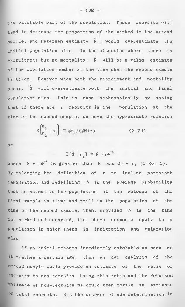
102

the catchable part of the population. These recruits will

tend to decrease the proportion of the marked in the second

sample, and Petersen estimate N , would overestimate the

initial population size. In the situation where there is

recruitment but no mortality, N will be a valid estimate

of the population number at the time when the second sample

is taken. However when both the recruitment and mortalityA

occur, N will overestimate both the initial and final

population size. This is seen mathematically by noting

that if there are r recruits in the population at the

time of the second sample, we have the approximate relation

By enlarging the definition of r to include permanent

immigration and redefining <P as the average probability

that an animal in the population at the release of the

first sample is alive and still in the population at the

time of the second sample, then, provided <t> is the same

for marked and unmarked, the above comments apply to a

Population in which there is immigration and emigration

also.

If an animal becomes immediately catchable as soon as

it reaches a certain age, then an age analysis of the

second sample would provide an estimate of the ratio of

recruits to non-recruits. Using this ratio and the Petersen estimate of non-recruits we could then obtain an estimate

°f total recruits. But the process of age determination is

(3.29)

or

E[N |n±] ^ N + r<P

where N + r<p 1 is greater than N and <£N + r, (0 <<p< 1).

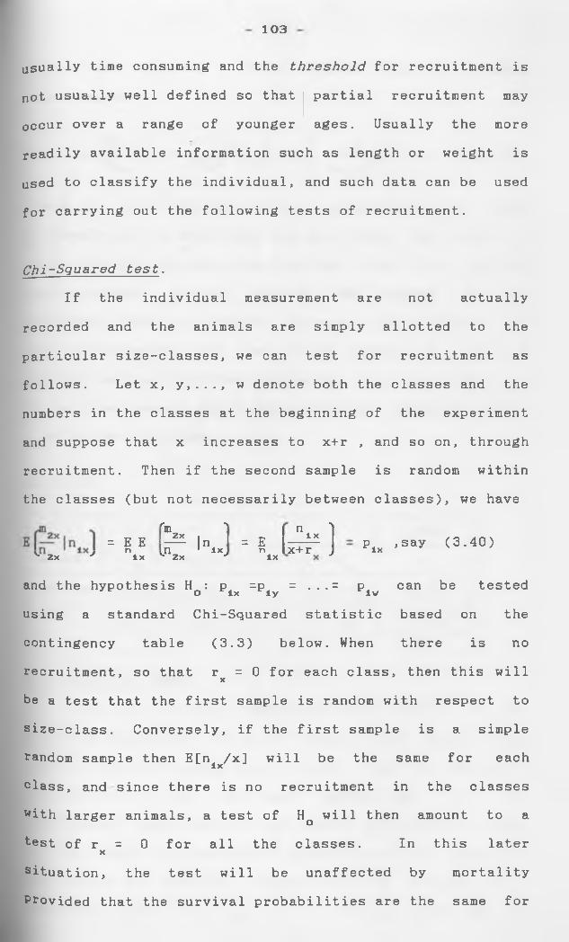
103

usually time consuming and the thr e s h o l d for recruitment is

not usually well defined so that partial recruitment may

occur over a range of younger ages. Usually the more

readily available information such as length or weight is

used to classify the individual, and such data can be used

for carrying out the following tests of recruitment.

C h i - S q u a r e d t e s t .

If the individual measurement are not actually

recorded and the animals are simply allotted to the

particular size-classes, we can test for recruitment as

follows. Let x, y,..., w denote both the classes and the

numbers in the classes at the beginning of the experiment

and suppose that x increases to x+r , and so on, through

recruitment. Then if the second sample is random within

the classes (but not necessarily between classes), we have

Plx > say (3.40)~~ P

fm2x

In l n J = * |1 n ‘ x ] lx + r JK Z x J l x L 2x lx

and the hypothesis H : p =p = ...= p, can be testedO lx ly lvusing a standard Chi-Squared statistic based on the

contingency table (3.3) below. When there is no

recruitment, so that r = 0 for each class, then this willX

be a test that the first sample is random with respect to

size-class. Conversely, if the first sample is a simple

random sample then E[n /x] will be the same for eachlxclass, and since there is no recruitment in the classes

with larger animals, a test of Hq will then amount to a

test of r = 0 for all the classes. In this laterX

situation, the test will be unaffected by mortality Provided that the survival probabilities are the same for

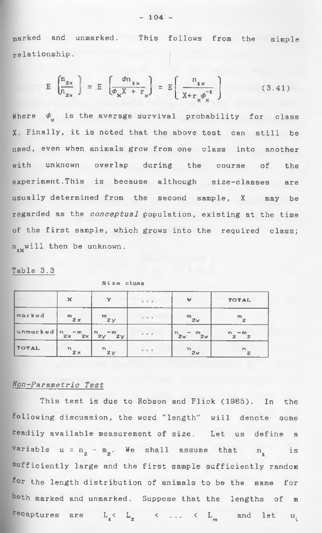
marked and unmarked. This follows from the simple

relationship.

- 104 -

K * 1 - E f 0n- 1 - T? n.x ]k x J k x +

— Cix+r J

(3.41)

Where <p is the average survival probability for class

X. Finally, it is noted that the above test can still be

used, even when animals grow from one class into another

with unknown overlap during the course of the

experiment.This is because although size-classes are

usually determined from the second sample, X may be

regarded as the con c e p t u a l population, existing at the time

of the first sample, which grows into the required class;

nixwill then be unknown.

Table 3.3S i z e c lass

X Y w T O TAL

mar k e d m m m m2 x 2 y 2v 2unmar k ©d n — m n — m n — m n — m2x 2x 2y 2y 2v 2v 2 2T O TAL n n n n2 x 2 y 2 v 2

No n - P a r a m e t r i c Test

This test is due to Robson and Flick (1965). In the

following discussion, the word “length" will denote some

readily available measurement of size. Let us define a

variable u = n„ - in . We shall assume that n is

sufficiently large and the first sample sufficiently random

^°r the length distribution of animals to be the same for

both marked and unmarked. Suppose that the lengths of m

recaptures are L < Lo < ... < L and let u.1 2 m t

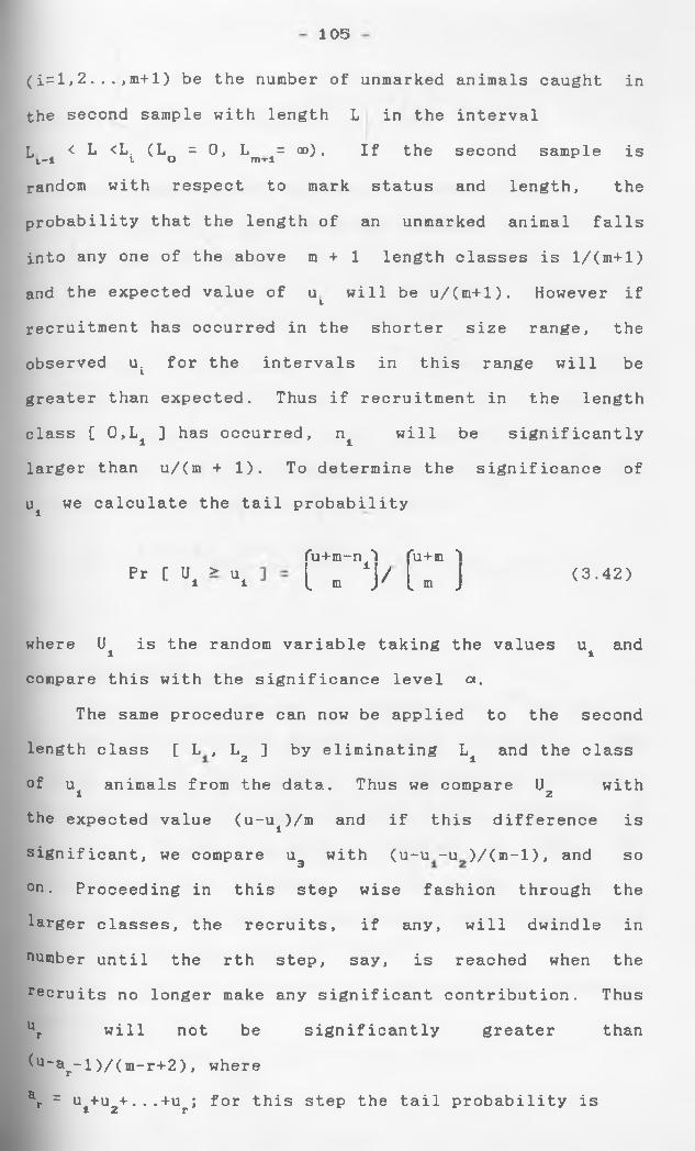
105

(i=l,2 ...,m+ 1 ) be the number of unmarked animals caught in the second sample with length L in the interval L < L <L. (L = 0, L =oo). If the second sample is

1,-1 l O THt I

random with respect to mark status and length, the probability that the length of an unmarked animal falls into any one of the above m + 1 length classes is l/(m+l) and the expected value of u l will be u/(m+l). However if recruitment has occurred in the shorter size range, the observed ui for the intervals in this range will be greater than expected. Thus if recruitment in the length class [ 0,Li ] has occurred, n£ will be significantly larger than u/(m +1). To determine the significance of u± we calculate the tail probability

Pr [ U± > u±f u + m - n / l f u + m I[ m J / [ m J (3.42)

where Ui is the random variable taking the values u± andcompare this with the significance level ot.

The same procedure can now be applied to the secondlength class [ L , Lz ] by eliminating L± and the classof u animals from the data. Thus we compare U with1 2the expected value (u-ui)/m and if this difference is significant, we compare u3 with (u-u -u )/(m-l), and so°n. Proceeding in this step wise fashion through the larger classes, the recruits, if any, will dwindle in number until the rth step, say, is reached when the recruits no longer make any significant contribution. Thus ur will not be significantly greater than(u~ar-l)/(m-r+2 ), wherear = u+u +...+U ; for this step the tail probability is1 2 r

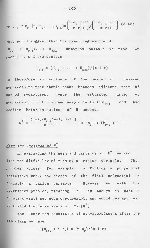
106

This would suggest that the remaining sample of U + U +...+ U unmarked animals is free ofr+l r+2 m+1recruits, and the average

Ur+l (Ur+l

is therefore an estimate of the number of unmarked

non-recruits that should occur between adjacent pair of

marked recaptures. Hence the estimated number of

non-recruits in the second sample is (m +1)0 „ and the

modified Petersen estimate of N becomes

N*<n+l){Ur + i(m+l) +m+l}

m + 1 <n4 +l)[0 r+ 1 + 1 ] - 1

*Mean and Variance o f N . *

*In evaluating the mean and variance of N we run

into the difficulty of r being a random variable. This

problem arises, for example, in fitting a polynomial

regression where the degree of the final polynomial is

strictly a random variable. However, as with the

regression problem, treating r as though it were a

constant would not seem unreasonable and would perhaps lead

to a slight underestimate of Var[N ].

Now, under the assumption of non-recruitment after the

rth class we have

E[Ur+i |m, r ,ar] = (u-ar)/(m+l-r )

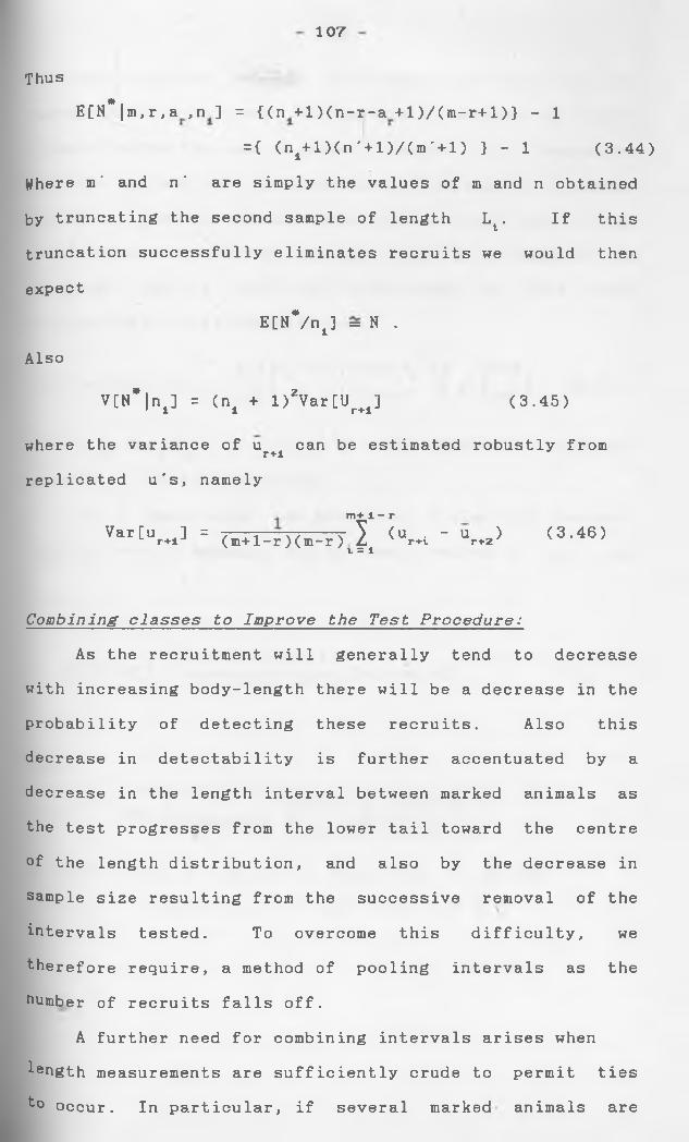
107

ThusE[N*|m,r,a ,n ] = {(n +l)(n-r-a +l)/(m-r+l)} - 1

= { (ni+l)(n' + l)/(m' + l) } - 1 (3.44)Where m' and n' are simply the values of ra and n obtained by truncating the second sample of length Lt. If this truncation successfully eliminates recruits we would then expect

E[N*/nJ = N .Also

V[N*|nt] = (n, + l)2Var[Ur+l] (3.45)

where the variance of u „ can be estimated robustly fromr+ireplicated u's, namely

m+ 1 - rVar[u ] =r+1 (m+l-r)(m=F7 1 (uv = 1 r+i - U r+2> (3.46)

C o m b i n i n g c l a s s e s to I m p r o v e the Test P r o c e d u r e :

As the recruitment will generally tend to decrease with increasing body-length there will be a decrease in the probability of detecting these recruits. Also this decrease in detectability is further accentuated by a decrease in the length interval between marked animals as the test progresses from the lower tail toward the centre of the length distribution, and also by the decrease in sample size resulting from the successive removal of the intervals tested. To overcome this difficulty, we therefore require, a method of pooling intervals as the number of recruits falls off.

A further need for combining intervals arises when iength measurements are sufficiently crude to permit ties to occur. In particular, if several marked animals are

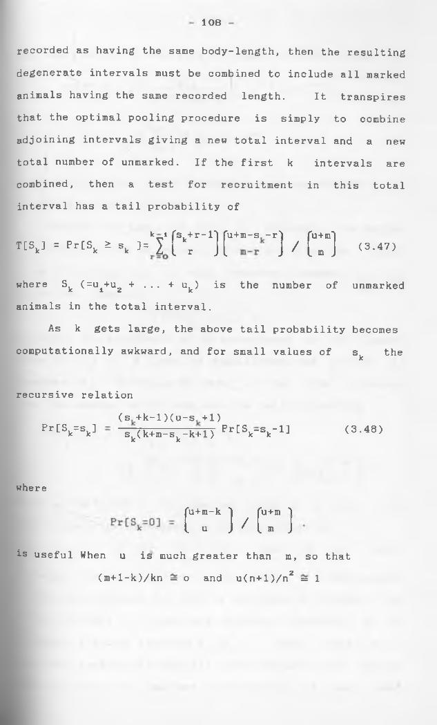
108

recorded as having the same body-length, then the resulting

degenerate intervals must be combined to include all marked

animals having the same recorded length. It transpires

that the optimal pooling procedure is simply to combine

adjoining intervals giving a new total interval and a new

total number of unmarked. If the first k intervals are

combined, then a test for recruitment in this total

interval has a tail probability of

kT'1 fsk+r_:H fu+m-s -r'') fu+mlT[Sk] = Pr£Sk * ■„ J* 2 L r Jl J / L J (3.47)

where sk < = V U2 + ••• + V is the number of unmarkedanimals in the total interval.

As k gets large, the above tail probability becomes

computationally awkward, and for small values of s thek

recursive relation

Prt W(s +k-l)(u-s +1) sk( k+m-sk-k+l) Pr^Sk"sk-1^ (3.48)

where

[u+m-k I fu+m ‘'Iu J / U J

is useful When u is much greater than m, so that

(m+l-k)/kn = o and u(n+l)/n2 = 1

109

the napplication of Stirling's formula to (3.48) gives

rm+1Pr[Sk > « ] ak m+l-k D

i = i v y

where p-(sk+k-1)/n. This incomplete beta approximation to

(3.48) holds for all K > 1 .

Suppose now that, the first intervals, the second

k2 intervals, and so on are combined to give new length

class [0,L ),[L , L ),... with unmarked numbers S,, S,1 1 2 1 J c k 2and so on. Then if

Pr[Sk > Sk]< al

We reject the hypothesis of no recruitment in the length

class [0, Lk) at ot level of significance and proceed to i

consider Sk . Dropping the date in the first interval2

from the sample, we now evaluate the tail probability

T[Sk ,Sk ] = Pr[Sk > sk |Sk =sk ] 2 1 2 2 1 1

■ 2 ( T 1) r ) / ( ? ■ )

where m'= m-k and u' u-S# are new values of m and u.We1 Kiagain reject the hypothesis of no recruitment in

, Lk ] if for Sk , Sk , and so on until 1 2 2 1

non-significance is achieved. The number of non-recruits

xn the second sample can then be estimated as before. One

the problems in combining adjacent intervals is to

datermine the best sequence k , k2, . .. since there is a

Practical possibility that all the recruits are smaller

(shorter) than the smallest non-recruit, it would seem

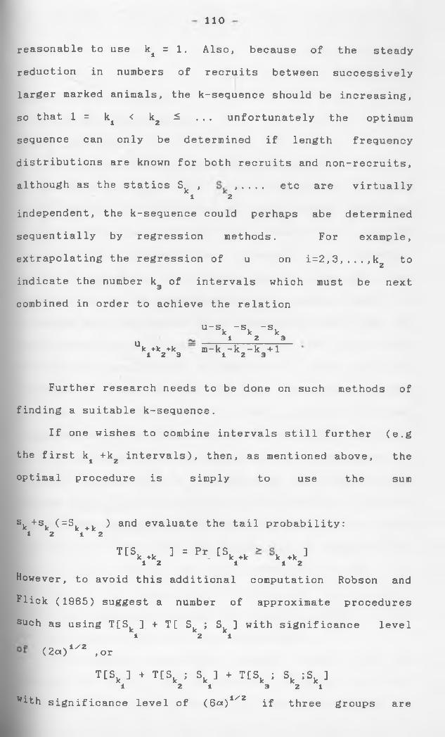
110

reasonable to use k± = 1. Also, because of the steady

reduction in numbers of recruits between successively

larger marked animals, the k-sequence should be increasing,

so that 1 = ki < k2 ^ ... unfortunately the optimum

sequence can only be determined if length frequency

distributions are known for both recruits and non-recruits,

although as the statics Sk , , . . . . etc are virtually1 2

independent, the k-sequence could perhaps

sequentially by regression methods,

extrapolating the regression of u on

indicate the number k of intervals which3combined in order to achieve the relation

uu-s -s. -s,k k k 1 2 3

k+k+k m-k -k -k +11 2 3 1 2 3

abe determined

For example,

i=2,3,...,k2 to

must be next

Further research needs to be done on such methods of

finding a suitable k-sequence.

If one wishes to combine intervals still further (e.g

the first k4 +k2 intervals), then, as mentioned above, the

optimal procedure is simply to use the sum

Sk +sk ^= k + k anc* ev&luate the tail probability:1 2 1 2T[SU . ] = Pr [S. . > . ]k +k - k +k k +k1 2 1 1 2

However, to avoid this additional computation Robson and

flick (1965) suggest a number of approximate procedures

such as using T[Sk ] + T[ Sk ; Sk ] with significance level1 2 1

( 2ot)1/2 , or

T[Sk ] + T[Sk ; Sk ] + T[Sk ; Sk ;Sk ]1 2 1 3 2 1

with signif icance level of (6ot)1/2 if three groups are

Ill

poo led.

Assumption II, III a nd I V l . P r a c t i c a l c o n s i d e r a t i o n s

variable calchability .

One of the crucial assumptions underlying the theory

of section 3.1, is that the second sample is a simple

random sample. Strictly speaking, such a random sample can

only be obtained by numbering the animals 1,2,...,N and

using a table of random numbers to select n animals.2

However, in practice, if all the animals have the same

catchability, we can approximate to a random sample by

arranging that every point of the population area has the

same probability of being sampled and that all points

selected are sampled with the same effort. If a more even

coverage is required one can use stratified random

sampling, whereby the population area is divided into equal

sub-areas and one or more points are allotted at random

within each sub-area. Unfortunately the requirement of

constant probability of capture may not hold, either

because of an inherent variation in catchability or because

catching and handling in the first sample affect future

catchability. Very often the probability of capture will

vary between various sub-groups defined by age, sex,

species, etc, for example certain sub-groups may be more

mobile and have different habitat preference, while others

may have certain bait and trap preferences.

In f isheries, catchability usually varies with thesize of the f ish, and considerable research has been

carried out on such problems as gear selectivity and

112

length-selection curves. When recruitment and mortality

are negligible and the marked members are individually

identifiable, then the randomness of the second sample with

respect to size can be tested by partitioning the first

sample into that portion which is ultimately recaptured and

into the portion which is not (Robson ,1969).

A Mann-Whitney rank-sum test comparing these two

sub-samples with respect to body size will be a test for a

monotonic ration between body size and probability of

capture in the second sample. Alternatively, if the marked

members are allotted to size-classes one can carry out the

goodness-of-fit test described earlier. When there is

variation in the inherent catchabilities of individuals and

the first sample is not random, assumption II will be false

and the more catchable individuals will be caught in the

first sample. This means that for the second sample, the

marked will in general be more catchable than the unmarked,

and assumption IV will be false. Unfortunately, apart from

a careful choice of catching method and preliminary studies

-for example, on activity, feeding habits, length-selection

curves, etc -little can be done to overcome this problem of

variable catchability in the first sample. However we

shall see below that the bias in the Petersen estimate N

due to variation in catchability can be reduced by using

different trapping methods for the two samples.

If the catchability is constant within certain

well-defined sub-groups and there are sufficient recaptures

from each sub-group, the numbers in each sub-group should

estimated separately.

113

S y s t e m a t i c S a m p l i n g :

We have seen that the Petersen estimate can still be

used, even when assumption IV is false and a systematic

rather than a random sample is taken, provided there is

uniform mixing of marked and unmarked and all animals are

catchable in the second sample. But in many populations

uniform mixing is unlikely because of territorial behaviour

on animals and the presence of well-defined home ranges.

Another situation where it is difficult to obtain a uniform

mixing is when the population is not randomly distributed

throughout the population area and animals are relatively

immobile. For example Hancock (1963) suggested that the

excessive variability in the monthly returns of marked

Whelks may have been due to the random distribution of

marked individuals among essentially non-randomly

distributed unmarked individuals.

It would seem that where possible the experimenter

should aim for a random sample rather than rely on the

assumption of uniform mixing. However in many population

studies it is helpful to arrange the release of the first

sample so that mixing can take place as much as possible.

For example, one can divide up the total area into

sub-areas,sample each sub-area with same effort, and then

release the marked animals back into the same area from

which they were taken. If catchability is independent of

sub-area, one would hope that this method produces roughly

the same proportion of marked in each sub-area. To check

this, a standard goodness-of-fit test can be carried out to

See whether the proportion of marks recorded in the second

sample from the various sub-areas are signif icantly

114

different.

C a t c h i n g and H a n d l i n g :

Departures from assumption III that trapping and marking do not affect catchability can be minimized if the following points are observed by the experimenter.

i. Type o f t r a p .

It is essential that a trapping method be used which will not harm the animal in any way. For example, in small mammal populations such things like placing the trap under cover of vegetation, drugging the bait, and visiting traps frequently can reduce trap mortality. If several types of traps are available one would endeavour to choose the type which is most efficient, as the accuracy of Petersen estimate increases with n and n„. Also to increase trap efficiency, the bait or lure should be selective for the species under investigations and some consideration should be given to the spacing and distribution of the traps. ii.

i i . M e t h o d o f h a n d l i n g .

Care is needed in handling the captured animals sothat they quickly recover on their return to the

%Population. Another problem arises with small mammals and birds where trap a d d i ction or trap s h y n e s s can alter an animals' pattern of behaviour after it has been caught for the f irst time. The effect of trap shyness can be minimized by prebaiting the traps for a suitable period of time before the census, thus allowing the animals to get used to

115

the presence of traps. This however does not always work and of course trap addiction is not helped by prebaiting-

Sometimes trap addiction can be reduced by altering the

trap positions throughout the trapping period, thus, for

example, preventing individuals from building their runways

up to the mouth of the trap. Another way of minimizing the

effect of trap response is to use a different trapping

method for taking the second sample. For example animals

can be live-trapped for marking and then shot for

recapture; if the mark is conspicuous, sight of the mark

itself could be the means of r e c a p t u r e. In the later case,

observing animals and noting the proportion of marked

amounts to sampling with replacement, so that Bailey s

binomial model is appropriate.

In some circumstances the tag itself may affect the

longevity and behaviour of the animals. For example, jaw

tags on fish can interfere with feeding and thus affect

growth rate, while Petersen disk tags can make fish more vulnerable to gill nets through the net catching under the

disk. Another aspect of marking particularly relevant to

insects is that presence of conspicuous marks may well destroy an animal's natural camouflage and make it more or

less liable to predation. Also when animals are marked by a

method which relies on the sight of the collector then the

marked animals may tend to be collected more than the

unmarked. On the other hand, if the tags are not

conspicuous enough they may be overlooked, particularly if

one relies on huntsmen, fishermen, farmers, and so on to

return the tags.

116

jiii. M e t h o d of r e l e a s e :

Animals often show a high level of activity

immediately on release, and efforts should be made to

minimize this. For example, birds and insects could

perhaps be restrained from flying immediately by covering

them with small cages until the effects of handling wear

off. While tagged fish could be held in tanks so as to

reduce and measure initial tagging mortality. If animals

have activity during the day they could perhaps be released

during an active period.

Theoretical a n a l y s i s o f c a t c h a b i l i t y

For the ith member of the population (i=l,2,..., N),

let x i be the probability that it is caught in n±, let

yt be the conditional probability that it is caught in n2

given that it is caught in n and let z. be the1 tconditional probability that it is caught in n2 given

that it is not caught in n . Assuming that the population

represents a random sample of N triples (xi,yi,zi) with

regard to the species as a whole and the particular method

used, then (xt, y. ,zt) may be regarded as a random

observation from a trivariate probability density function

(f„(x,y,z), say. If we set a.=n.-m (the number of animals1 v i 2caught in the ith sample, only, i=l,2), then the

Probability of a given outcome of the whole experiment.

p __J r ■>

a + a 1 2

’’a +a + m 1 2 2

TT *(i.-y.) TT a - x t)z. TT x ky kII L l=a1+1 J k = a + a +1 ^ 1 2 ^

xNTT (i-xl)ci-zl>

l = a + a + m +1 1 2 2

117

Therefore the conditional probability function of a±, a2,m1 is

f (a ,a ,m !x.,y.,z.) = ) P2 X l ’ 2' l 1 r L vV

where 1 denotes summation over all possible groups of

the N animals such as a , a2, mz are the numbers in

each of the three categories, that is w represents a

permutation of N objects such that aA fall in the first

category, and so on. Since the triple (xt, y , z ) are

independent they can be integrated out and thes'*unconditional probability function is given by

f 3( a l > a2 ,ml ) = E f 2( a l , a 2 j ini|xi , y . , z . )

= 1 E cp„ ] = 1 < p , - P i 2 > ‘ <p3- P i 9> 2a - p r p 9+pls >N - a -n.

where

]> 1 = N!/{ai!a2!mi!(N-ai-n2)!}

and p± = E[x], pg = E[z], p±3 = E[xz], and p±2 =E[xy],

all expectations being with respect to f . Now

f5(a2’mZlni> = f3(ai'a2’ni> / W

f n 1 f p 1m

2 r P o l a i f N - n 1r _ _ \

P - P J#1i * 12

i 12i 3 13

K J Lp » Ji

p * j l a * J 1 - p * J

fl-p “P ~P * 1 3 13

1 - P

N-n -a 1 2

and approximating these two binomial distributions by two

- 118 -

independent Poisson distribution we have (Feller,1957)✓V *\

f<,("2 lni’n2) =nm2y. j

m n -mP 2(1-P) 2 2

where

P= n± / ((N-n±)k + n±} , k=^P3_P13>P1 / (P^d-Pi)}

Therefore, it can be shown that

E[N*|ni,nz] = { (nl+l)/P }{ (l-(l-P) * } -1n +1 2

= n/P =( N-n± )k + n ±*so that N is approximately unbiased estimate of N if and

only if k = 1. Suppose that assumption III is true. Let

wherek = (B-pi)/(l-pi)

B=p (p -p +p )/p1 3 13 12 ' * 1 2

obviously k = 1 if and only if B = 1 and k < B when

B <1. Since assumption III is true, that is marking does

not affect catchability, we have

y. = z. ( i=l, 2, . . .N)

so that P 13= pl2 , P3 = p2. and

1-B = 1-p p /p 1 2 12

= (p -p p )/p

= Cov[x,y]/E[xy]

suppose, now that B = 1, then, Cov[x,y]/E[xy] = 0

°r Cov[x,y] = 0- and Cov[x,y] = 0 if and only if x and

y are uncorrelated. Thus B= 1 if and only if x and y are

uncorrelated.

A positive correlation will lead to an underestimate

N and a negative correlation will lead to an

0verestimate of N . We note that if a correlation exists we

119

would generally expect it to be positive. This accounts

for the persistent underestimation observed by Buck and

Thoits (1965) who checked on several estimates of fish

population numbers by draining the ponds containing the

populations.

We conclude from the above that variation in

catchability due to, say trapping selectivity could exist

for both samples without introducing biase of the source of

selectivity in two samples were independent. This supports

the statements by a number of authors that bias due to

difference in catchability can be reduced by using a

different sampling method for each sample.

Special c a s e :

Let y =bx^ ( b >0 ). Here the correlation is unity

and we find that

B = l-Var[x]/{E[x]}2 S 1,

with equality if and only if Var[x] = 0 or x is

constant.

If x e [c,d] ( 0 ^ c < d ^ 1) then, provided W=c/d

is not too small, it can be shwon that B will be nearer

unity and insensitive to the shape of f(x), the probability

density of x.

On the other hand if c=0, B may be significantly

less than unity; if in addition f(x) is concentrated near

x=0, that is the probabilities of capture are near zero for

a substantial proportion of the population, then B could

still be much smaller. In this case x and y are

uncorrelated if either x or y is constant, that is B=1

If at least one of the two samples is a random sample. In

120

particular if the first sample is random, the second sample

peed not be random and in fact could be highly selective,

provided the selectivity was independent of mark status.

When x is constant we find that p =p p , p =p p13 1 3 12 1 2

and k=p3/p2< This means that k=l if and only if the

average probability of capture of the marked in the second

sample is the same as the average for the unmarked.

We see from the above discussion that if Assumption

III is true and y^=bx^, then k =1 if and only if

Assumption II is true. A test for this case based on

taking two samples from a known (for example, marked)

population is given below. Conversely, if Assumption II is

true then k=l if and only if Assumption III is true.

Test for constant c a t c h a b i l i t y

We shall now consider the problem of testing

Assumption I given that the assumptions I, II, III, V and

VI are true, by taking 3 samples and using the first sample

as an identifiable population.

Suppose that m2 tagged animals in the second sample

are given another tag and the second sample then returned

into the population. If a third sample of size ng is now

taken then on the basis of the tagging information obtained

and assuming that catching and tagging do not effect future

catchability, Cormack (1966) gives two procedures, one of

which we discuss below, for testing the hypothesis of

constant catchability.

In the following discussion we note that n , n£ and

n3 play the same role as N, n , n2 in theoretical

analysis of the previous section above.

121

The probability pj (j=1,2,...,n±) that the jth

members of the first sample is captured in a later sample

will be proportional to its inherent catchability and to

the intensity of sampling or sampling effort. Assuming the

sampling effort f to be the same for each individual, we

therefore define c =P/f as the catchability of the jth

individual for the particular catching method used. We

shall assume that cv's to be a random sample of size n4

from a probability density function g(c) with moments /u'

about the origin and moments v about the mean. If werstandardise c so that the domain of g is [o,l], then

f will be uniquely determined and 0 5S f ^ 1. The

catchability of an animal may be regarded as the

probability with which it places itself in a position where

the experimenter is able to catch it; and the sampling

intensity is then the probability that an animal in this

position will be caught. Alternatively, if c is not

standardised, we can regard it as the probability that one

unit of sampling effort catches the jth individual. Then

considering f as the number of units of effort to be

additive, p. = fc. as before. Let f and f be theJ J 2 3sampling efforts for samples two and three respectively.

Then if and yj are the probabilities that the jth

member of sample one is caught in samples two and three

respectively, and assuming assumption III is true, we have: -

x.= f c., y.=f c., and hence y =bx.J 2 J J 9 J J Jhet in be those individual caught in the first sample,10

®12 those caught in both samples one and two only, mi3,

those caught in both samples one and three only, and mi23

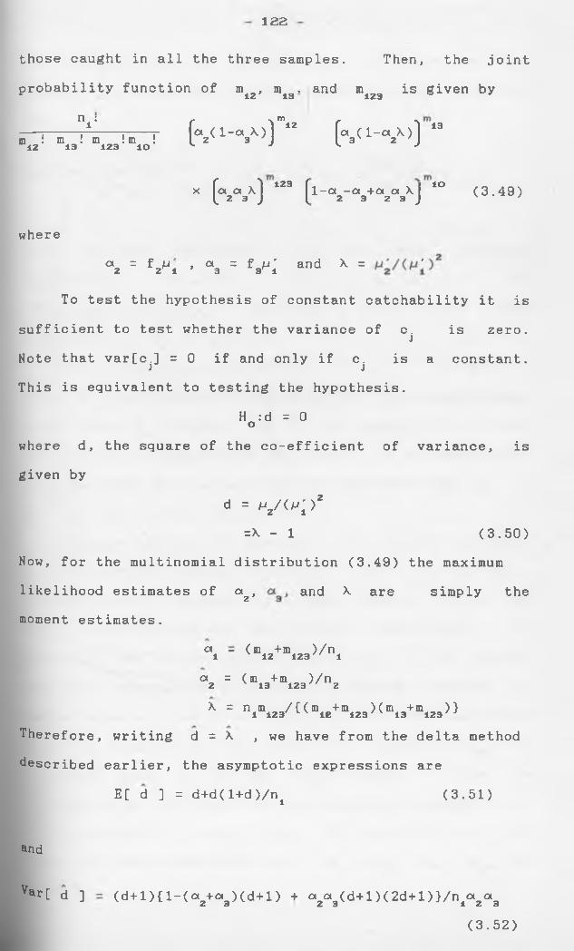
122

those caught in all the three samples. Then, the joint

probability function of in , m . and m is given by12 13 123

n ; 1( « 2 < i - * 3 x > r i 2 ( V 1- 2X>)m !12 m ! m ! m !

13 123 l O

X ( C,2 0,3 X ) 12 3 (1 - a - a 4-a a X 1 2 3 2 3 J

13

lO (3.49)

where*a2 = f2M i ' "a = f3 ^ and x =

To test the hypothesis of constant catchability it is

sufficient to test whether the variance of c. is zero.jNote that varCcp = 0 if and only if c is a constant.

This is equivalent to testing the hypothesis.

H :d = 0 owhere d, the square of the co-efficient of variance, is

given by

a = *v<^>2=\ - 1 (3.50)

Now, for the multinomial distribution (3.49) the maximum

likelihood estimates of c*2, and X are simply the

moment estimates.

Theref ore, writing

described earlier,

a - (m +m )/n1 V 12 1 2 3 " 1

°2 = (mi3+m!23)/n2

X = n1m123/{(”.2+%23)<m.3+mi23>>d = X , we have from the delta method

the asymptotic expressions are

E[ d ] = d+d(l+d)/nA (3.51)

and

Var[ d ] (d+l){l-(a2+a3)(d+l) + ot2ot3(d+l)(2d+l)}/niot2a3

(3.52)

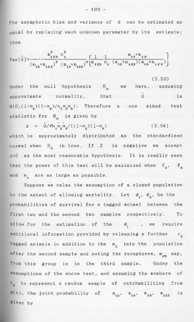
123

The asymptotic bias and variance of d can be estimated as

usual by replacing each unknown parameter by its estimate;

thus

mVar[d]= 1 2 3

n

(m +m ) (m +mV 12 1 2 3 13 123

- {— ■~ N 2 1 m n) ^ 1 2 3 1

m +m12 1 3

(m +m )(m +m )V 12 1 2 3 ' ' 13 1 2 3 ;

(3.53)Under the null hypothesis Hq we have, assuming

approximate normality, that d is

N( 0, ( 1-a )( l-« )/n a a ) ■ Therefore a one sided test

statistic for Hq is given by

z = d/Vn^otg/Ul-c^Kl-otg) (3.54)

which is approximately distributed as the standardized

normal when Hq is true. If Z is negative we accept

d=0 as the most reasonable hypothesis. It is readily seen

that the power of this test will be maximized when f2, fg

and n are as large as possible.

Suppose we relax the assumption of a closed population

to the extent of allowing mortality. Let <P±, <P2> be the

probabilities of survival for a tagged animal between the

first two and the second two samples respectively. To

allow for the estimation of the 4> , we require

additional information provided by releasing a further r2

tagged animals in addition to the mz into the population

after the second sample and noting the recaptures, m23 say,

from this group is in the third sample. Under the

assumptions of the above test, and assuming the members of

r2 to represent a random sample of catchabilities from

S(c), the joint probability of mi2, mi3, m23, mi23 is

Siven by

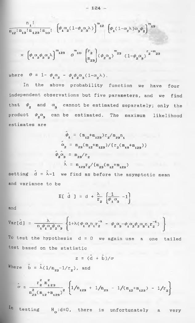
124

n l • r -v 'T* r -vTn-- ni— rz-- rr— , °<_(1-0 a X.) \<p ( 1 -a X)a <p 1II112!mi 3 !,ni2 3 !miO! >- ‘ 2 ” J l * 2 3 2J

[i m m<p a <p a xl 123 0 101 2 2 3 J m

2 3v — ./

™ r -mx 2 3 . 2 2 3

(*2V

where 0 = 1- ^>a - <p <p a (1-a X).1 2 ^1~2 3 v 2 yIn the above probability function we have four

independent observations but five parameters, and we find that 4>z and cannot be estimated separately; only theproduct <P2a3 can be estimated. The maximum likelihood estimates are

\ = (mi2+%23)r2/[n23ni

“ 2 = m 23<m i2+ n i 2 3 > / t r 2 ( m i3+ m i23>>A A

<p a = m / r2 3 23 2A

X = m r /{m (m +m )12 3 2.' L 2 3 ' 12 1 2 3 '

A A

setting d = X-l we find as before the asymptotic mean and variance to be

E[ d ] = d* h f e - . 1

and

Var[d] = n <p a <p a1 1 2 2 3

1+X(fan r ± - < p a - < p a < p c i n r ±) i-1 2 1 2 2 3 * 1 2 * 2 3 1 2 '

To test the hypothesis d = 0 we again use a one tailed test based on the statistic

2 = (d + b )/aWhere b = X( l/m2 3-l/r2) , and

2 2 .. r m f- = — - 123 2 jl/n

m (m +m )2 3 12 1 2 3 ^ ^

” 123 + v®,, - 1 A " 12+">123) - 1 /■1

In testing HQ :d=0, there is unfortunately a very

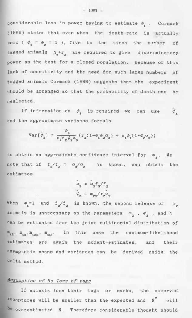
125

considerable loss in power having to estimate <p± . Cormack

(1966) states that even when the death-rate is actually

zero ( - <P2 - 1 ), five to ten times the number of

tagged animals n1+r2 are required to give discriminatory

power as the test for a closed population. Because of this

lack of sensitivity and the need for such large numbers of

tagged animals Cormack (1966) suggests that the experiment

should be arranged so that the probability of death can be

neglected.

If information on 4>± is required we can use <P± and the approximate variance formula

<PVar[<P ] - ----4— {r (1-<P <p a ) + n <t> (1 -<p a )}i n r <P cn L 2V 1 2 3 y i^iv * 21 2 2 3

to obtain an approximate confidence interval for 4> . We

note that if ^3/ ^ 2 = is known, can obtain theestimates

a = a f /f3 2 3 / 2

A A

<t> - m / r c*.2 23y 2 3When <P±-1 and fg/f2 is known, the second release of r2

animals is unnecessary as the parameters a , <p . and X2 2

can be estimated from the joint multinomial distribution of

, m43,®i23 * m10* this case the maximum-likelihoodestimates are again the moment-estimates, and their

asymptotic means and variances can be derived using the

delta method.

Assumption o f No loss o f tags

If animals lose their tags or marks, the observed

recaptures will be smaller than the expected and N* will

overestimated N. Therefore considerable thought should

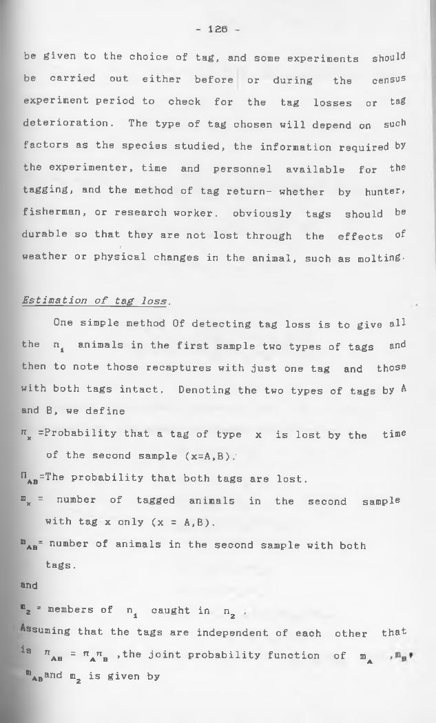
be given to the choice of tag, and some experiments should

be carried out either before or during the census experiment period to check for the tag losses or tag

deterioration. The type of tag chosen will depend on such

factors as the species studied, the information required by

the experimenter, time and personnel available for the

tagging, and the method of tag return- whether by hunter*

fisherman, or research worker. obviously tags should be

durable so that they are not lost through the effects of/

weather or physical changes in the animal, such as molting-

E s t i m a t i o n o f tag l o s s .

One simple method Of detecting tag loss is to give all

the n animals in the first sample two types of tags and

then to note those recaptures with just one tag and those

with both tags intact. Denoting the two types of tags by A and B, we define

nx =Probability that a tag of type x is lost by the time

of the second sample (x=A,B).‘

nAB=The probability that both tags are lost.

nx = number of tagged animals in the second sample with tag x only (x = A,B).

mAB= number of animals in the second sample with both tags.

and

m2 = members of n caught in n1 2ssuming that the tags are independent of each other that

ls nAB = nA nB »the joint probability function of mA

mABanc* m2 Is £iyen by

- 126 -

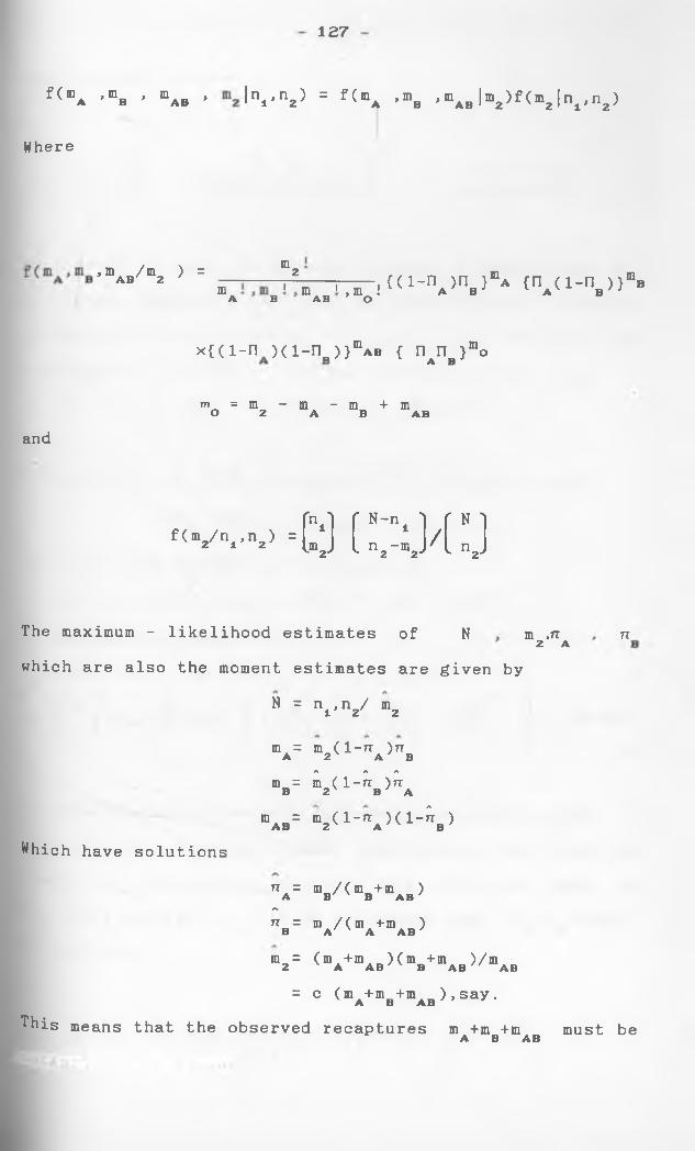
1Z7

f(mA ,mB , mAB , ln»*n»> = f(mA ’% '“a. I V ^ I ' V ' V

Where

* ^ “2 5 = m > m , , m ! { ( i - n A )nB }»A {nA( i - n B ) } “BA B AB O

x{(i-n )d-n„)}mAB { n n _ }moA B

and

m = m - m - m + m O 2 A B AB

f < w v = £ ; ] ( i ; j / [ : j

The maximum - likelihood estimates of N

which are also the moment estimates are given by

N = nj,n2/ m2

m ,n2 A 77

m A= in (1-77 )77A 2 x A / BA A A

% = m2(1-nB>’IA% B = ” 2< 1 - " A K 1 - ^ B )

Which have solutions

"a = V < V " a b >A.

"B = “A/(mA+mAB>

m2= (mA+lnAB)<mB + mAB>/mAB= c (mA+mB+mAB),say.

^his means that the observed recaptures m +m +mA B AB must be

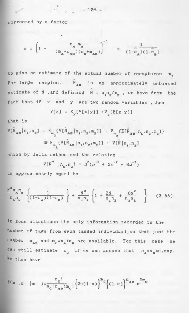
128a - ■'

corrected by a factor

■ [ -

m mA B( 11 A+mAB > ( BB + lnAB ,]

- 1

to give an estimate of the actual number of recaptures m .2

For large samples, NAB is an approximately unbiased

estimate of N ,and defining N = n n /m * we have from the

fact that if x and y are two random variables ,then

V[x] = Ey[V[x|y 3] +Vy[E[x|y]]that is

= Em + Vm {E[Nab 1 ^ , 1 ^ ] }2 2

= \ W » a.Iw b23> +

which by delta method and the relation

V[N* |nt,n2] = NZ(a/_1 + 2v~2 + 6aj~3) is approximately equal to

M3N n nA Bn n 1 2

I-* __i

l + N9 11 1 2N . 6N2 ]l _nA) ( 1-™ b ) J n .n2 n in2 n in2 J

(3.55)

In some situations the only information recorded is the

number of tags from each tagged individual,so that just the

number m • and m =m +m_ are available. For this case weA d C A B

Can still estimate m if we can assume that n =rr =n, say.Z A Bthen have

_ m l r \m \in 2m<m |m )=,°c!mAB !m0! {2rt( 1-71}} c{ a - " ) } AB « ‘

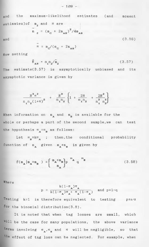
129

and the maximum-likelihood estimates (and moment

estimates)of m2 and n are

and

m = (m + 2m ) /4m2 V C A B ' ' A B

" = m C / ( m C + 2 m A B )

(3.56)

Now setting

SAB * n,BA <3-57>The estimate(3.57) is asymptotically unbiased and itsasymptotic variance is given by

»i 3 2N nn in2(l+rr)<

+ 1 + 2Nn in2

+

When information on m and m is available for theA B

whole or perhaps a part of the second sample,we can test

the hypothesis n =n as follows:A B

Let tt =krr ; then,the conditional probabilityD A

function of m given m +m is given byA A B

(3.58)

Where

Testing k=l is

the b inomial

It is noted

will be the case

terms involving

the effect of tag

k ( 1 _ 7 T A )TTAP = j— ----x-- ;--- Tk--- \ and p = l-qk(l-n*)nA+ nA (l-»A )

therefore equivalent to testing p=i/2

distribution(3.8).

that when tag losses are small, which

for many populations, the above variance

n ,n and tt will be negligible, so thatA B

loss can be neglected. For example, when

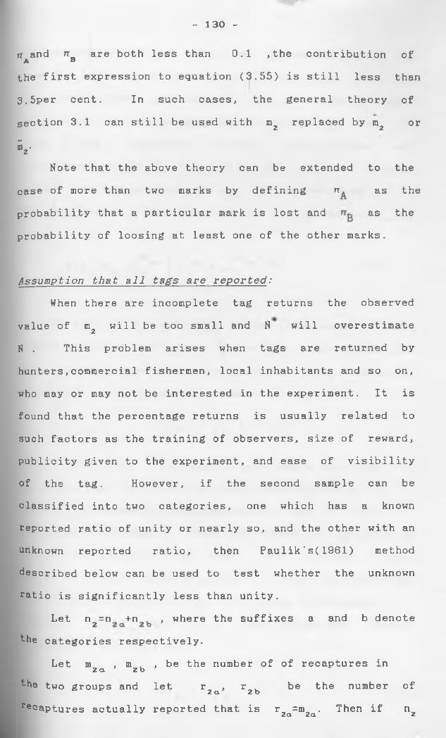
n and n are both less than 0.1 ,the contribution ofA Bthe first expression to equation (3.55) is still less than

3.5per cent. In such cases, the general theory of

section 3.1 can still be used with m replaced by m or2 2

N

■VNote that the above theory can be extended to the

case of more than two marks by defining n as the

probability that a particular mark is lost and as the

probability of loosing at least one of the other marks.

- 130 -

Assumption that all tags are r e p o r t e d :

When there are incomplete tag returns the observed

value of m will be too small and N will overestimate2

N . This problem arises when tags are returned by

hunters,commercial fishermen, local inhabitants and so on,

who may or may not be interested in the experiment. It is

found that the percentage returns is usually related to

such factors as the training of observers, size of reward,

publicity given to the experiment, and ease of visibility

of the tag. However, if the second sample can be

classified into two categories, one which has a known

reported ratio of unity or nearly so, and the other with an

unknown reported ratio, then Paulik's(1961) method

described below can be used to test whether the unknown

ratio is significantly less than unity.

Let n =n +n , where the suffixes a and b denote

the categories respectively.

Let m , m , be the number of of recaptures in2 a 2 b

the two groups and let r , r , be the number of2 a 2 b

recaptures actually reported that is r2a=m2a* Then if n2

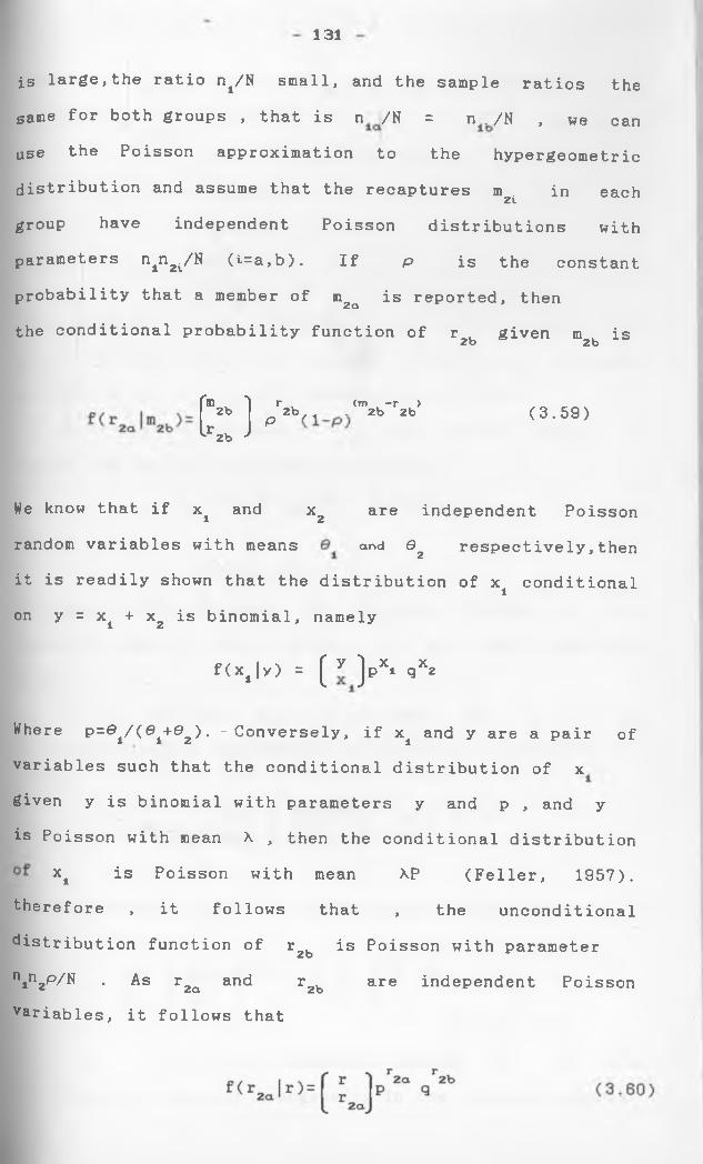
131

is large,the ratio n^/N small, and the sample ratios the same for both groups , that is n /N = n ./N , we canuSe the Poisson approximation to the hypergeometricdistribution and assume that the recaptures m in each2igroup have independent Poisson distributions withparameters n^n^/N (i=a,b). If p is the constantprobability that a member of m2a is reported, thenthe conditional probability function of r given m is2b 2b

[m . "1 r (m -r >2b f 2b, „ . 2b 2br I p 2b J

(3.59)

We know that if x and x2 are independent Poisson random variables with means and Q respectively,thenit is readily shown that the distribution of x± conditional on y = x± + x2 is binomial, namely

f ( x j y ) = ( * ) p x . q xa

Where p=0±/( ei+e2) • - Conversely, if x± and y are a pair of variables such that the conditional distribution of x given y is binomial with parameters y and p , and y is Poisson with mean X , then the conditional distribution

x± is Poisson with mean XP (Feller, 1957). therefore , it follows that , the unconditional distribution function of r2b is Poisson with parameter nin2p/N ■ As r2a and r2b are independent Poisson Variables, it follows that

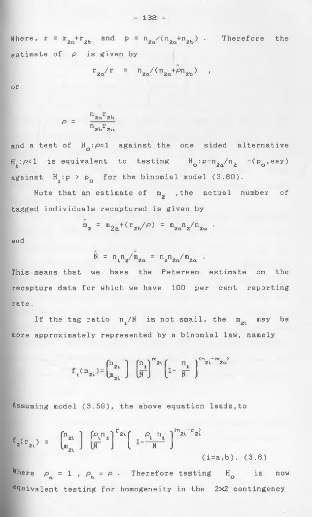
132

Where, r = r2<j+r2b and p = n2a/( n2c+n2b ) . Therefore the

estimate of p is given by

r2d/r = n2a/(n2a+^n2b) -or

P = n2ar2bn2br2a

and a test of HQ :p=l against the one sided alternative

H :p<l is equivalent to testing Hq :p=n2a/n2 =(P0*say)

against H^p > p q for the binomial model (3.60).

Note that an estimate of m2 ,the actual number of

tagged individuals recaptured is given by

andm2 = B2a+(r2b/P) = V 2/nza •

N = nin2/m2a = n,n2a/m2aThis means that we base the Petersen estimate on the

recapture data for which we have 100 per cent reporting

rate.

If the tag ratio n±/N is not small, the m2i may be

more approximately represented by a binomial law, namely

. < ■ » > = £ : ] G O - r )<n -m >

2 i 2 a

Assuming model (3.59), the above equation leads,to

f ( 2'* . > ■ t ] r - n - V s )<n-r >

2l 2l

(i=a,b). (3.6)

is nowNhere P a = 1 , Pb = P • Therefore testing Hq

ec3uivalent testing for homogeneity in the 2x2 contingency

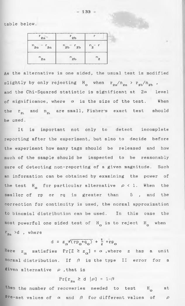
133

table below.

r r r2a ’ 2bn - r n - r n - r2a 2a 2b 2b 2

n n . n2a 2b 2

As the alternative is one sided, the usual test is modified

slightly by only rejecting Hq when r2a/ n 2a > r2b//n2b ' and the Chi-Squared statistic is significant at 2a level

of significance, where a is the size of the test. When

the r . and n . are small, Fisher's exact test should2l 2i

be used.

It is important not only to detect incomplete

reporting after the experiment, but also to decide before

the experiment how many tags should be released and how

much of the sample should be inspected to be reasonably

sure of detecting non-reporting of a given magnitude. Such

an information can be obtained by examining the power of

the test H for particular alternative p < 1. When the osmaller of rp or rq is greater than 5 , and the

correction for continuity is used, the normal approximation

to binomial distribution can be used. In this case the

most powerful one sided test of Hq is to reject Hq when

r2a >d , where

d = z "/(rp +q ) + - + rp a v 2 oHere z satisfies Pr[Z ^ z ] = a ,where z has a unit a anormal distribution. If ft is the type II error for a

Siven alternative p ,that is

Pr[r2a > d |p] = 1-ft

then the number of recoveries needed to test Ho at

Pre-set values of a and ft for different values of P

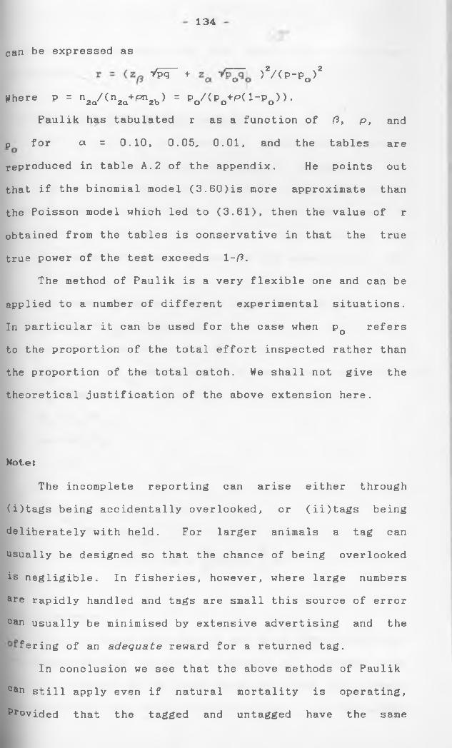
134

can be expressed as

1 - <- z ftypg_ + z a >2/<P-P0)ZWhere p = n2a/(n2o+Pn2b) = P0/(P0+P( 1-P0 ) ) •

Paulik has tabulated r as a function of ft, p, and

p for a = 0.10, 0.05, 0.01, and the tables are

reproduced in table A.2 of the appendix. He points out

that if the binomial model (3.60)is more approximate than

the Poisson model which led to (3.61), then the value of r

obtained from the tables is conservative in that the true

true power of the test exceeds 1-ft.

The method of Paulik is a very flexible one and can be

applied to a number of different experimental situations.

In particular it can be used for the case when pQ refers

to the proportion of the total effort inspected rather than

the proportion of the total catch. We shall not give the

theoretical justification of the above extension here.

Note:

The incomplete reporting can arise either through

(i)tags being accidentally overlooked, or (ii)tags being

deliberately with held. For larger animals a tag can

usually be designed so that the chance of being overlooked

is negligible. In fisheries, however, where large numbers

are rapidly handled and tags are small this source of error

can usually be minimised by extensive advertising and the

fering of an a d e q u a t e reward for a returned tag.

In conclusion we see that the above methods of Paulik

Can still apply even if natural mortality is operating,

Provided that the tagged and untagged have the same

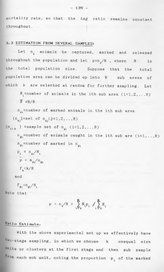
135

mortality rate, so that the tag ratio remains constant throughout.

3.3 ESTIMATION FROM SEVERAL SAMPLES:Let n i animals be captured, marked and released

throughout the population and let p=nt/N , where N is

the total population size. Suppose that the total

population area can be divided up into R sub areas of

which k are selected at random for further sampling. Let

N.=number of animals in the ith sub area (i=l,2,...R) N =N/R

nit=number of marked animals in the ith sub area

(nij} = set of n±j( 0=1,2, . . ,R)

{nitk } =sample set of (i=l,2,...R)

n2.=number of animals caught in the ith sub are (i=l,..,R)

n =number of marked in n .Zl 2lp. = n ,/N.

t ll V

P = m2i/n2if ^ k / R

and

f_. =n /N.Zl 2l lNote that

P = n4/N N

^gtlo Estimate.

With the above experimental set up we effectively have

two-stage sampling, in which we choose k unequal size

Ur*its or clusters at the first stage and then sub sample

^rom each sub unit, noting the proportion p o f the marked

136

in each sub sample. Therefore, if the cluster sizes N

were known, p could be estimated by the ratio type

estimator

1 W j Ni •

However, as the IT are known, one possibility is to use

weights proportional to the sample sizes n . , so that p2vis estimated by

i

and N is estimated by n ±/p , the Petersen estimate once

again.lt is noted that

= 1 n2lPi / "2 <3 ‘62)

We now consider two cases where p is unbiased and

approximately unbiased respectively.

Constant M a r k R a t i o :

When p = p ( i = l, 2, . . . , k) the right-hand side of

(3.62) is reduced to p and p is unbiased. In this caseA A

Var[p|{n }] , the variance of p can be estimated by

V±[p] = P(l-p)/(n2-l)

The hypothesis Ho :pt=p can be tested using the standard

goodness-o-fit statistic

9 = Z <n2i"n2ip )Vn2lP(l-P)-i = 1Which when H is true is o approximately distributed as

Chi-Squared with k-1 degrees of freedom. When Ho is**rue and n2 is large (say, greater than 30). p is

aPproximately normal with mean p and variance estimate

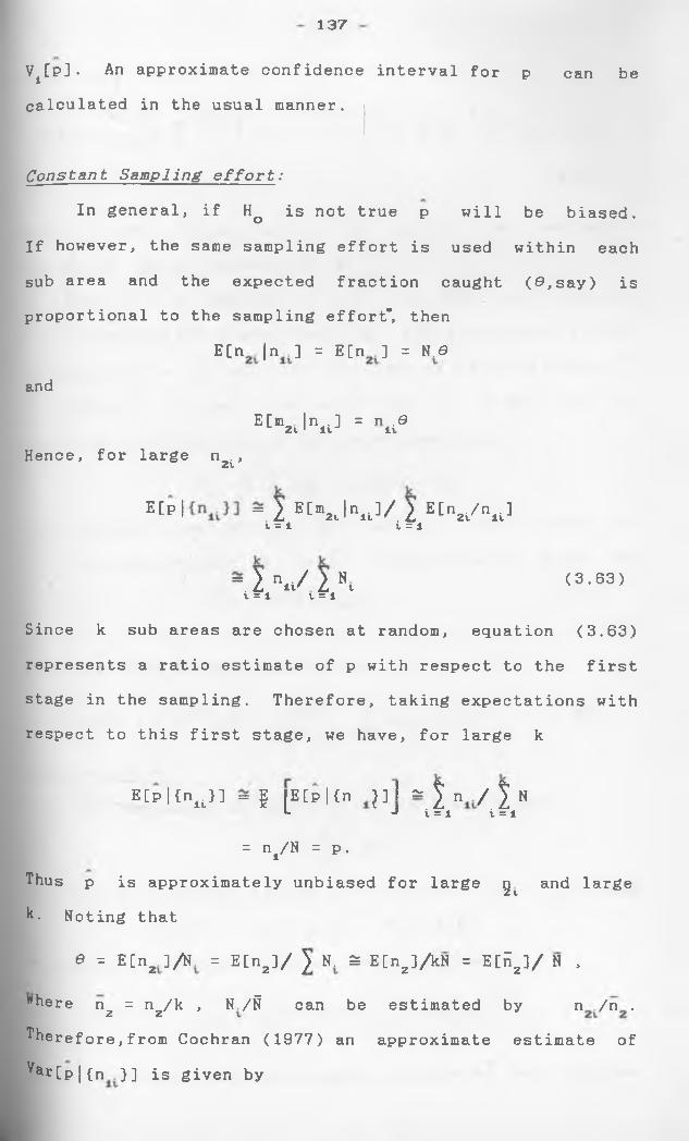
137

Vl[p]• An approximate confidence interval for p can be

calculated in the usual manner.

Constant S a m p l i n g e f f o r t :

In general, if Hq is not true p will be biased.

If however, the same sampling effort is used within each

sub area and the expected fraction caught (0,say) is

proportional to the sampling effort*, then

E [n | n ] = E [n ] = N.0

and

E[m In . ] = n .02l 1 It ItHence, for large n2i,

E C p | = 2 E C “ 2 i l n , i V 2 E [ n 2 i / n i t ]i = l i = l

= } n.-/ > N. Li it' L t (3.63)t = i t = i

Since k sub areas are chosen at random, equation (3.63)

represents a ratio estimate of p with respect to the first

stage in the sampling. Therefore, taking expectations with

respect to this first stage, we have, for large k

E[p|{nlt}] = | |E[p | {n J]1 * \ n / \ NL J i = l i = l

= n4/N = p.

Thus p is approximately unbiased for large gL and large k- Noting that

6 = E[nz.]/N. = E[n2]/ ]>N. Ss E[n2]/kN = E[H2]/ N ,

*here n2 = n2/k , N/fi can be estimated by n /n .

therefore,from Cochran (1977) an approximate estimate of

VarCp|{n }] is given by

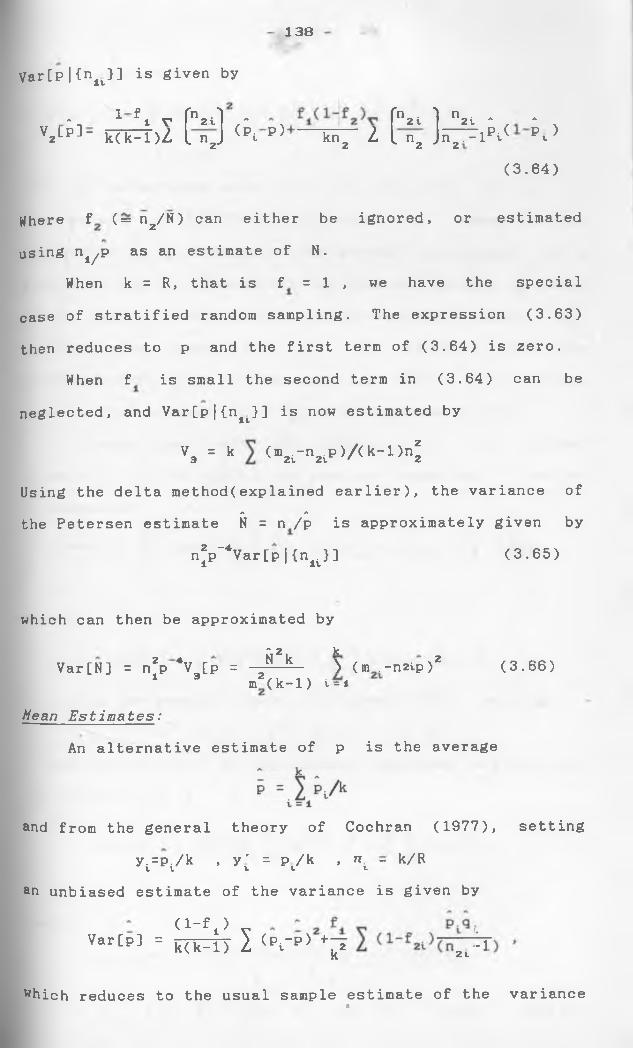
138

Var[p|(nit}] is given by

», 1 f l V fn2i) * fn2i *] n2i * *

V2 l-P-1- k( k -1 )Z [ n2J (pi p) kn2 Z [ n2 Jn2.-lpi/ P v ^

(3.64)

Where f (= nz/N) can either be ignored, or estimated

using n1//P as an estimate of N.When k = R, that is f = 1 , we have the special

case of stratified random sampling. The expression (3.63)

then reduces to p and the first term of (3.64) is zero.

When f is small the second term in (3.64) can be

neglected, and Var[p|{nit}] is now estimated by

va = k 1 <">2r n2ip)/(k-l)n^

Using the delta method(explained earlier), the variance ofA A

the Petersen estimate N = n /p is approximately given by

n^p”4Var [p | (nii)] (3.65)

which can then be approximated by"2 k

Var[N] = n2p 4V [p = k V (m .-naip)2 (3.66)1 3 m2< k-1) i = i

Mean E s t i m a t e s :

An alternative estimate of p is the average

and

an

from the general

v V k •unbiased estimate o

(l-f±) Var[p] = R F T )

theory of Cochran (1977),

y ' = p /k , n - k/Rl l tf the variance is given by

I <pr p > V 12l

setting

which reduces to the usual sample estimate of the variance L •

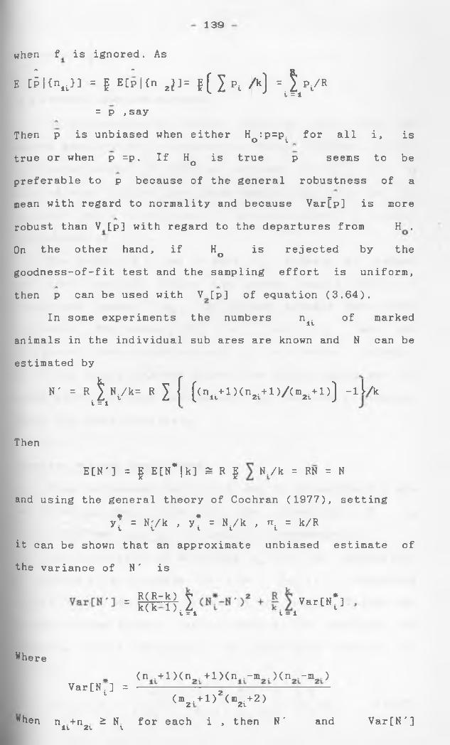
139

when f is ignored. Asa A n

E [5|{ntlJ] = | E[p|{n 2J] = | ( J p, A ) = J V rV y i = l= P ,say

Then p is unbiased when either HQ :p=p^ for all i, is

true or when p =p. If Hq is true p seems to be

preferable to p because of the general robustness of a

mean with regard to normality and because Varfp] is more

robust than V [p] with regard to the departures from H .

On the other hand, if Ho is rejected by the

goodness-of-fit test and the sampling effort is uniform,

then p can be used with V [p] of equation (3.64).

In some experiments the numbers n . of markeditanimals in the individual sub ares are known and N can be

estimated by

»' = Rt V k= R 1 f (<nu+lXn2l+l)/<m2t+l>) - l U

Then

E[N' ] = | E[N* | k] 2= R | N./k = RN = N

and using the general theory of Cochran (1977), setting

y* = Nr/k , y* = N./k , n. = k/Rt t t t tit can be shown that an approximate unbiased estimate of

the variance of N ' is

- 1 8 =8 . 1t = i t = iVar[N*]t

Where* (n . + l ) ( n „ + l ) ( n -m . ) ( n -m )

Var [N . ] = -------------------------------t ,, „ N 2Onz.+l) (m2t+2)

"hen n +n £ N for each i , then N' andIt 2t t Var [N']

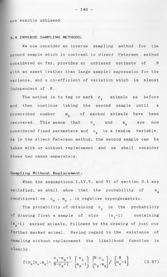
140

are exactly unbiased.

3 . 4 INVERSE SAMPLING METHODS.We now consider an inverse sampling method for the

second sample which in contrast to d i r e c t Petersen method

considered so far, provides an unbiased estimate of N

with an exact (rather than large sample) expression for the

variance, and a co-efficient of variation which is almost

independent of N.

The method is to tag or mark n± animals as before

and then continue taking the second sample until a

prescribed number m2 of marked animals have been

recovered. This means that n4 and m2 are now

considered fixed parameters and n is a random variable.2

As in the direct Petersen method, the second sample can be

taken with or without replacement and we shall consider

these two cases separately.

Sampling Without Replacement.When the assumptions I,IV,V, and VI of section 3.1 are

satisfied, we shall show that the probability of n2

conditional on n2 , mz , is negative hypergeometric.

The probability of obtaining n± is the probability

of drawing first a sample of size (ni~l) containing

(m2~l) marked animals, followed by the drawing of just one

further marked animal. Having regard to the existence of

sampling without replacement the likelihood function is

olearly

n -ra +1 r n 1 fN-n 1 r nf(n2 |nl>m2) = 1

m -1 1n -in / n2-l V2 l 2 J l 2 2 J

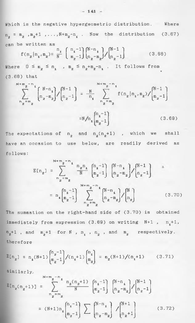
141

Which is the negative hypergeometric distribution. Where

n = in ,m+l , ...,N+m-n . Now the distribution (3.67)* 2 2 2 2 1

can be written as

(3.68) thatN+ m - n 2 1

n = m 2 2

n r ni -n ra-n. l fN-l 1ir ■ u - J k k J / n -1 <3-68> 2n2 S nL , ®2 - n +m0-n<i . 2 2 1 It follows from

•

N + m - nf N-nl ra-i 1 2

- + I

1 fN-i 'ik - " 2 / n 2 _ 1

f(n2|n1,m2)/ m -ix. 2 2J l 2 J n = m L 2 J2 2

(3.69)

The expectations of n2 and n2(n2+l) , which we shall

have an occasion to use below, are readily derived as

follows:N+ m - n 2 1

E[V - In = m

2 2

2 1

N+ m - n

ci£ rN-i i

( v 1.

in -in 2 2 k. J

/ D N1 ,

....

fn-11 2 1 fN-n 1=", m -1 Y n24 2 /

n 2l 2 J n = m l 2 2J l 2J(3.70)

2 2

The summation on the right-hand side of (3.70) is obtained

immediately from expression (3.69) on writing N+l , n+l,

n2+l , and mz+l for N , n± , nz , and m2 respectively.

therefore

fn -11 f OE[n2] = nl<H+l) 2

Lm2_1 l j/(nt+l) = m2(N+l)/(n1+l) (3.71)

similarlyx

E[n2(n2+1)] ' Y

N + m - n 2 12' 2N

n = m 2 2

rn -11 fN-n 1 H-l '

r s N1

V_______ i

n -n_L 2 2 J / n2-i

= (N+l )nfn -11 fN-n 1 "N+l 'i y i

/V 1-

L_. n -mL 2 2 J V 1.(3.72)

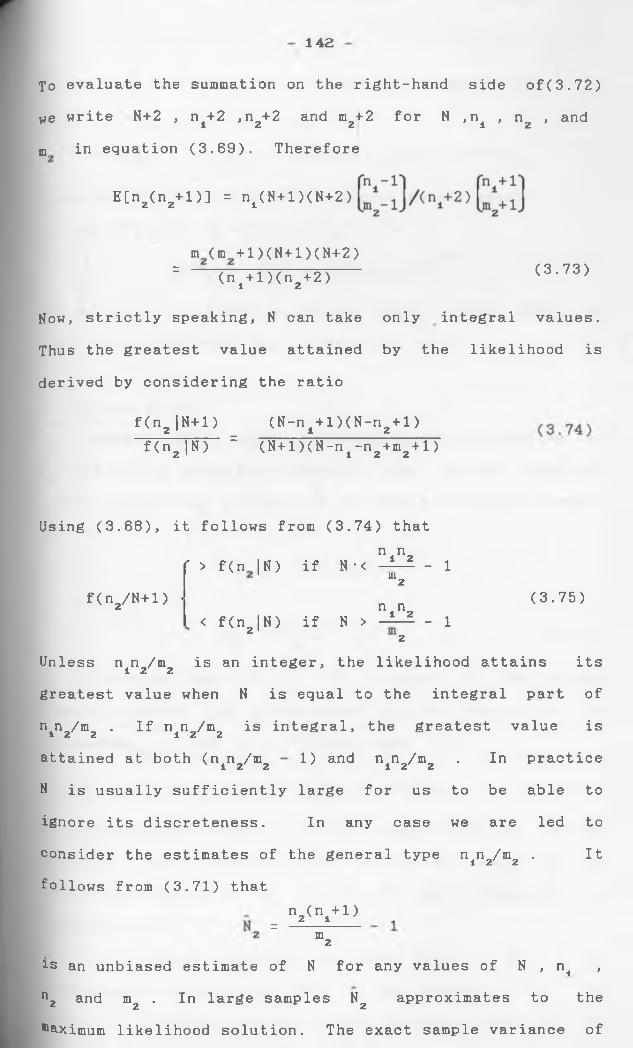
142

To evaluate the summation on the right-hand side of(3.72)

we write N+2 , n±+2 ,nz+2 and m2+2 for N ,n± , n z , and

m in equation (3.69). Therefore

E[n2(n2+1)] = n±(N+l)(N+2)

m (m +1)(N+l)(N+2)= (n. + l X n , ^ ) (3'73)

Now, strictly speaking, N can take only integral values.

Thus the greatest value attained by the likelihood is

derived by considering the ratio

f(nz |N+l) (N-nl+l)(N-n2+l)f(n2 |N) = (N+l)(N-nl-n2+m2+l)

Using (3.68), it

r

f(nz/N+l) h

follows from (3.74) thatn inz> f (n | N ) if N • < - 1m2

nin2< f(nz|N) if N > - 1(3.75)

2

Unless n n /m is an integer, the likelihood attains its 12 2greatest value when N is equal to the integral part of

nin2/m2 . If nin2/m2 is integral, the greatest value is

attained at both (n n /m12 2 1) and n n^/m, 12 2 • In practice

N is usually sufficiently large for us to be able to

ignore its discreteness. In any case we are led to

consider the estimates of the general type nin o/mo 2 2 • It

follows from (3.71) that

=n2<n,+ 1) ,

"ais an unbiased estimate of N for any values of N ' ni >

n2 and m2 . In large samples N2 approximates to the

Maximum likelihood solution. The exact sample variance of

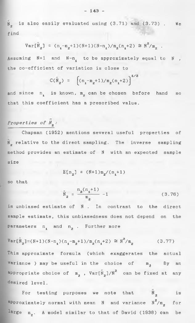
Nz is also easily evaluated using (3.71) and (3.73) . We

find

Var[N2] = (nl-n2+l)(N+l)(N-nl)/m2(nl+2) S N2/m2 .

Assuming N+l and N-n± to be approximately equal to N ,

the co-efficient of variation is close to

C(H2) = | (ni-m2+l)/m2(ni+2)J

and since n4 is known, m2 can be chosen before hand so

that this coefficient has a prescribed value.

- 143 -

P r o p e r t i e s of N 2 : * 1 2

Chapman (1952) mentions several useful properties of

Nz relative to the direct sampling. The inverse sampling

method provides an estimate of N with an expected sample

size

E[nz] = (N+l)m2/(ni+l)

so thatn (n +1)

N = — — ------ 12 m_

is unbiased estimate of N . In contrast to the

sample estimate, this unbiasedness does not depend

parameters n and n„ . Further more1 2

(3.76)

direct

on the

Var[N2] = (N+l)(N-ni)(nl-n2+l)/m2(n1+2) ^ N2/n2 (3.77)

This approximate formula (which exaggerates the actualvariance ) may be useful in the choice of m^ By an

* 2appropriate choice of m2 , Var[N2]/N can be fixed at any

desired level.

For testing purposes we note that N2 is2aPproximately normal with mean N and variance N /in for

2

*-arge m2. A model similar to that of David (1938) can be

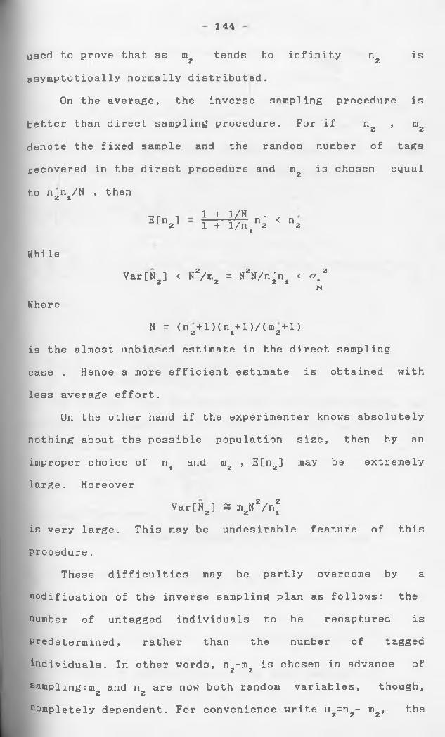
144

used to prove that as m tends to infinity n is2 2

asymptotically normally distributed.

On the average, the inverse sampling procedure is

better than direct sampling procedure. For if n2 , m2

denote the fixed sample and the random number of tags

recovered in the direct procedure and m2 is chosen equal

to n2nA/N , then

While

E[nz] 1 + 1/N ,1 + l / n ±n 2

< n2

Var[N ] < N2/m, = N2N/n'n < o-.2 2 2 2 1 N

Where

N = (n2+l)(ni+l)/(m2+l)

is the almost unbiased estimate in the direct sampling

case . Hence a more efficient estimate is obtained with

less average effort.

On the other hand if the experimenter knows absolutely

nothing about the possible population size, then by an

improper choice of nA and mz , E[nz] may be extremely

large. Moreover

Var[NJ S m N2/nf 2 2 1

is very large. This may be undesirable feature of this

procedure.

These difficulties may be partly overcome by a

modification of the inverse sampling plan as follows: the

number of untagged individuals to be recaptured is

Predetermined, rather than the number of tagged

individuals. In other words, n -in is chosen in advance of2 2

sampling:m and n are now both random variables, though, 2 2

completely dependent. For convenience write uz=n2~ m2, the

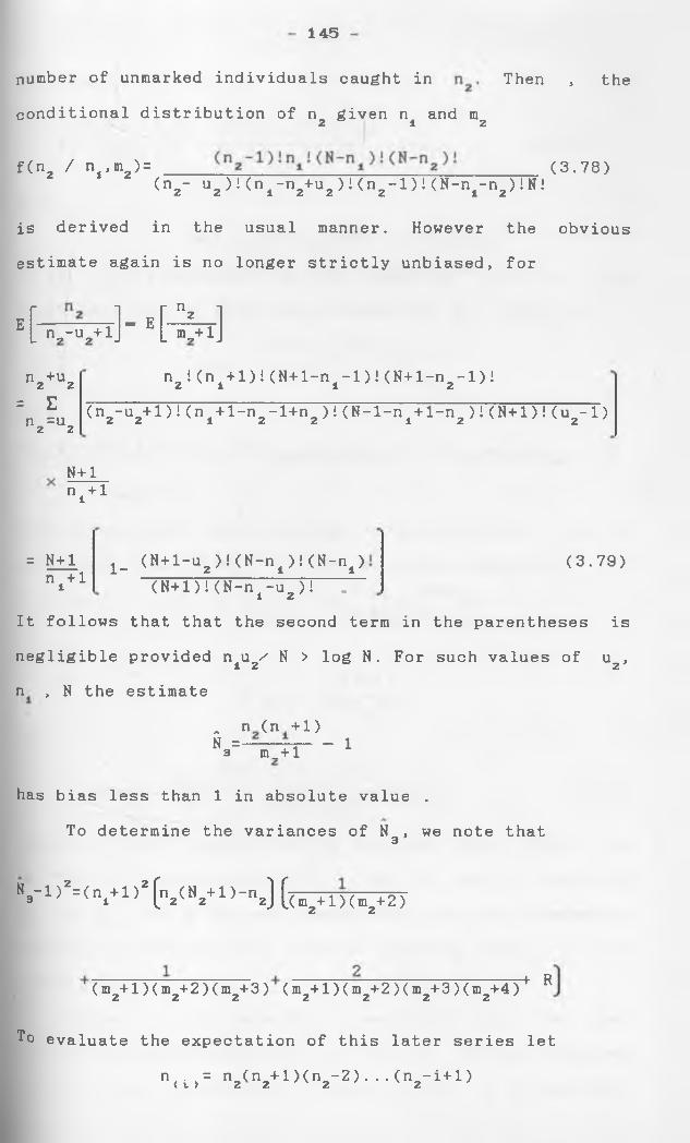
145

number of unmarked individuals caught in Then , the

conditional distribution of n given n and m2 1 2

f(n2 / ni,m2)= (3.78)(n2- u2)!(ni~n2+u2)!(n2_1)i (N-n1~n2)iN!

is derived in the usual manner. However the obvious

estimate again is no longer strictly unbiased, for

' [ w l - ' f e ]

n +uo 2 2

= En =u

2 2

n2 i(ni+l)!(N+1-ni-l)i(N+l-n2-l)i

(n2-u2+l)!(ni+l-n2-l+n2)!(N-l-ni+l-n2)!(N+l)!(u2-l)

N+l ni + !

= N+l.ni+1

x_ (N+l-u2 )!(N-ni)!(N-ni) (N+l)i(N-ni-uz ) ! I

(3.79)

It follows that that the second term in the parentheses is

negligible provided n4u2 N > log N. For such values of u2,

n , N the estimate

„ n (n +1)N = — --Ti--- 13 m_ + l

has bias less than 1 in absolute value .

To determine the variances of Ng, we note that

V l ) 2=(V l)2 (n2<N2+l)-nJ(;(mz+l)(m2+2)

(m2+1)(mz+2)(mz+3) (m2+1)(mz+2)(m2+3)(m2+4)+ R

To evaluate the expectation of this later series let

n<i>= n2< V 1)(n2-2)-•-(n2-i+1)

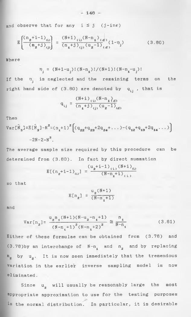
146

and observe that for any i ^ 3 (j-i=0

(3.80)

Where

If the r). is neglected and the remaining terms on theright hand side of (3.80) are denoted by q. . , that is'•j

The average sample size required by this procedure can be

determined from (3.80). In fact by direct summation

Either of these formulae can be obtained from (3.76) and

(3.78)by an interchange of N-n and n2 and by replacing

® by u . It is now seen immediately that the tremendous

variation in the earlier inverse sampling model is now

eliminated.

Since uz will usually be reasonably large the most

appropriate approximation to use for the testing purposes

is the normal distribution. In particular, it is desirable

Then

Var[N3]=E[N3]-S2=(ni+l)2

-2N-2-N2.

E[(n2+i-1>,i>]

so that

ECnz] ‘ (N-n'l+l)u 2(N+1>

and

Var[n ]= 2

u2n i(N+l)(N-u2-ni+l) ^ n ±(3.81)

<N-ni+l)z(N-nl+2)2 N ni

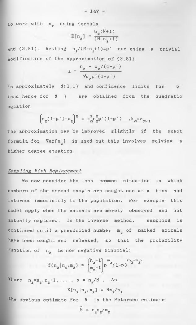
147

to work with n2 using formulau (N+l)

= (N-n +1)

and (3.81). Writing n±/( N-ni+1 )=p' and using a trivial

modification of the approximation of (3.81)

z = n2 " uz//( 1_p •/u2p ' ( 1-p ' )

is approximately N(0,1) and confidence limits for p'

(and hence for N ) are obtained from the quadratic

equation

[n2(l-p')-u2]2 = k2u2p'(l-p) ,ka =z01/2

The approximation may be improved slightly if the exact

formula for Var[n2] is used but this involves solving a

higher degree equation.

S a m p l i n g With R e p l a c e m e n t

We now consider the less common situation in which

members of the second sample are caught one at a time and

returned immediately to the population. For example this

model apply when the animals are merely observed and not

actually captured. In the inverse method, sampling is

continued until a prescribed number m2 of marked animals

have been caught and released, so that the probability

function of n^ is now negative binomial;

=h2- nm2-l

m <n -m >2/1 \ 2 2 P (1-P)

Where n2=m2,m2+l, . .. , p = n±/N . As

E[n2|n±,m2] = Nm2/n±

the obvious estimate for N is the Petersen estimate

N = n n /m

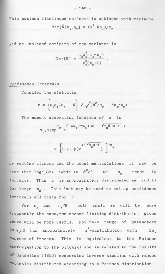
148

This maximum likelihood estimate is unbiased with variance

Var[N|ni,mz] = (N2-Nni)/m2

and an unbiased estimate of the variance is

Var[N] = nzni(n2~m2)

C o n f i d e n c e I n t e r v a l s .

Consider the statistic

z = f nin7 b, - N 2 2 / / ( N 2/m2 - Nn/m2)

The moment generating function of z ism ( pm / V m <l-p> - ~/m 0/<l-p> )w / / \ 2 2 2 2M (#)=p ez

p / V m <l-p> 1-tn.(l-p)e )

By routine algebra and the usual manipulations it may be2seen that logMz(0) tends to 0 /2 as m2 tends to

infinity. Thus z is approximately distributed as N(0,1)

for large m2 . This fact may be used to set up confidence

intervals and tests for N .

For m2 and n±/N both small as will be more

frequently the case,the second limiting distribution given

above will be more useful. For this range of parameters

2ntn2/N has approximately ^-distribution with 2mz

degrees of freedom. This is equivalent to the Poisson

aPproximation to the binomial and is related to the results

Sandelius (1950) concerning inverse sampling with random

Variables distributed according to a Poisson distribution.

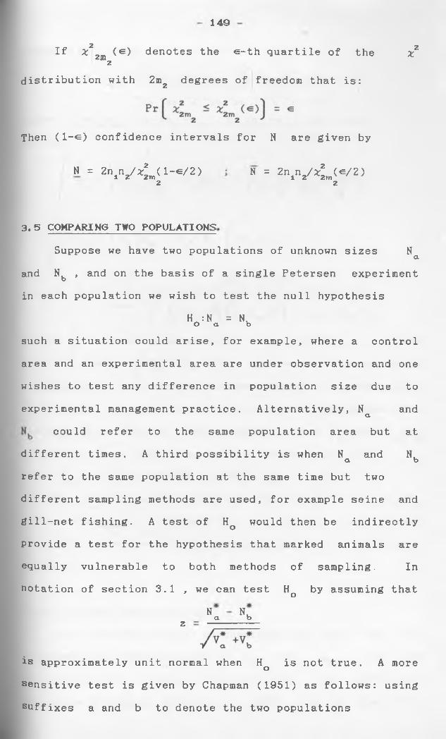
149

2If * (€ ) denotes the e-th quartile of the x2m ^2

distribution with 2mz degrees of freedom that is:

2

Then (1-e) confidence intervals for N are given by

« = 2n1n2/ ^ m <1-e/2 ) N = 2" * V 4 » « 2>2 2

3.5 COMPARING TWO POPULATIONS

Suppose we have two populations of unknown sizes Naand N, , and on the basis of a single Petersen experimentOin each population we wish to test the null hypothesis

H :N = NkO a bsuch a situation could arise, for example, where a control

area and an experimental area are under observation and one

wishes to test any difference in population size due to

experimental management practice. Alternatively, N andacould refer to the same population area but at

different times. A third possibility is when N and N,a brefer to the same population at the same time but two

different sampling methods are used, for example seine and

gill-net fishing. A test of Hq would then be indirectly

provide a test for the hypothesis that marked animals are

equally vulnerable to both methods of sampling. In

notation of section 3.1 , we can test Ho by assuming that

is approximately unit normal when Hq is not true. A more

sensitive test is given by Chapman (1951) as follows: using

suffixes a and b to denote the two populations

N NbaZ

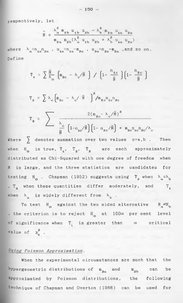
150

respectively, let

N =\2 \3 X m L u ^ u , - X , m u u a 2 b lb 2b b 2 a la 2a

2 2m m . ( X u . u . + X , u u )2a 2o a lb 2b b la 2aJwhere Xa=nlan2a , ula=nia-m2a , u2a=n2a-m2a ,and so on

Def ine

T. = I t ) / ( i - x H ‘ - y )

TZ * 1 \ (",< - V 8 ) /•z«"l.nK

Z 2(m - Xc/fi)2x------------- ---------------------

f(i-n^/S) [l- n2c/fi) + m2cnlcn2c/Xc

Where ^ denotes summation over two values c = a,b . Then

when Hq is true, T ±, T , Tg are each approximately

distributed as Chi-Squared with one degree of freedom when

N is large, and the three statistics are candidates for

testing H . Chapman (1952) suggests using T when X =XO 2 a o, T3 when these quantities differ moderately, and T±

when X is widely different from X .a t>To test H against the two sided alternative N *N.O a b

, the criterion is to reject Hq at lOOot per cent level

of significance when T. is greater than ct critical

value of x" .

Using P o i s s o n A p p r o x i m a t i o n .

When the experimental circumstances are such

hypergeometric distributions of in and m .2a 2bapproximated by Poisson distributions, the

technique of Chapman and Overton (1966) can be

that the

can be

following

used for

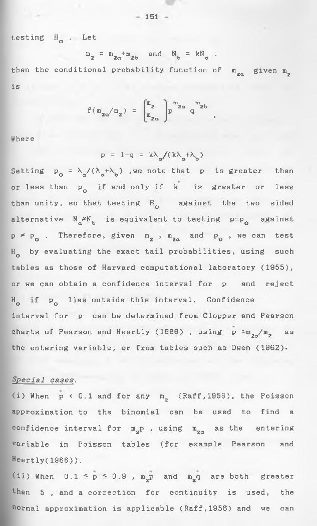
151

testing Ho Let

m = m +m2 2a 2b

and N = kN .b a

then the conditional probability function of m2a

given id2

is

m2 m m 2a 2bp q >f ( m 2a / n 2 ) =

c.m

2a J

Where

p = 1-q = kX /(kX +Xw)a ' a b

Setting po = X /(X +X ) >wea a o

note that p is greater than

or less than P if and only if o»k is greater or less

than unity, so that testing Ho against the two sided

alternat ive N *N. is equivalent to testing p:CL O =po against

p * pD • Therefore, given m , 2 ’ U 2a & n d PC > we can test

Hq by evaluating the exact tail probabilities, using such

tables as those of Harvard computational laboratory (1955),

or we can obtain a confidence interval for p and reject

H if p lies outside this interval. Confidence o ointerval for p can be determined from Clopper and Pearson

charts of Pearson and Heartly (1966) , using p =m /m as2 CL 2

the entering variable, or from tables such as Owen (1962).

Special c a s e s .

(i) When p < 0.1 and for any mz (Raff,1956), the Poisson

approximation to the binomial can be used to find a

confidence interval for in p , using in as the entering2 2d

variable in Poisson tables (for example Pearson and

Heartly(1966 ) ) .

(ii) When 0.1 ^ p ^ 0.9 , mzp and mzq are both greater

than 5 , and a correction for continuity is used, the

normal approximation is applicable (Raff,1956) and we can

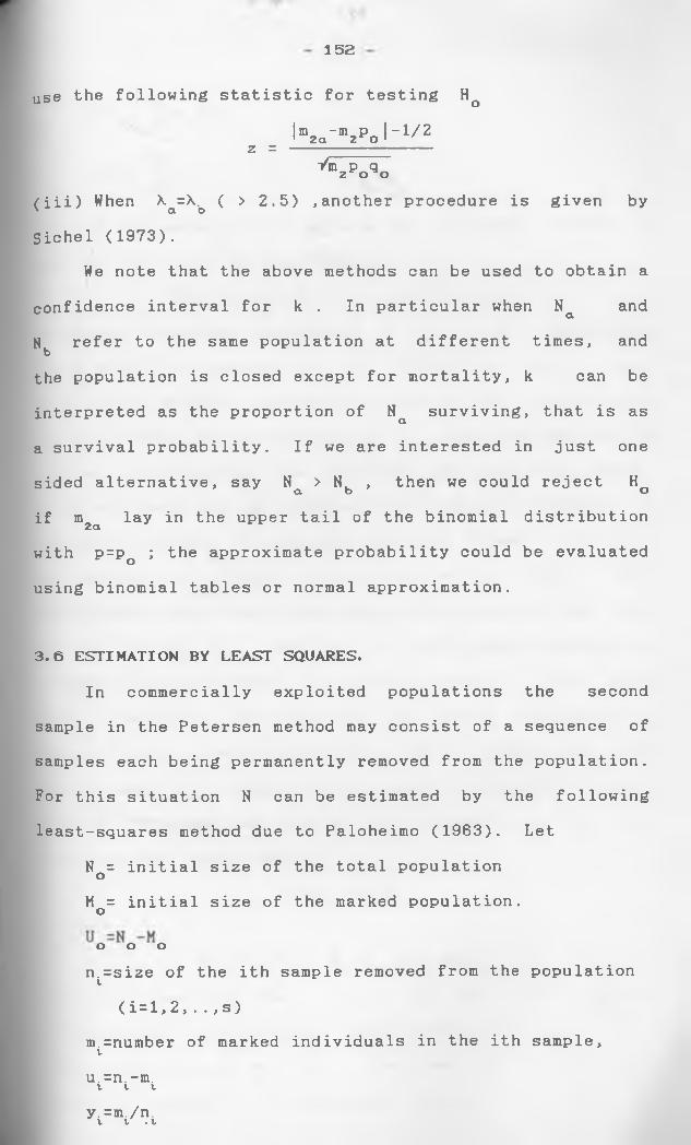
152

use the following statistic for testing Hq

K a ‘m2Pol~1/2 Z = -------------"/m p q 2 0 0

(iii) When X =V ( > 2.5) ,another procedure is given by' C l D

Sichel (1973).

We note that the above methods can be used to obtain a

confidence interval for k . In particular when Nq and

N refer to the same population at different times, and bthe population is closed except for mortality, k can be

interpreted as the proportion of N surviving, that is asCla survival probability. If we are interested in just one

sided alternative, say N > N. , then we could reject Ha. b O

if m lay in the upper tail of the binomial distribution2 ciwith P=PQ ; the approximate probability could be evaluated

using binomial tables or normal approximation.

3.6 ESTIMATION BY LEAST SQUARES.In commercially exploited populations the second

sample in the Petersen method may consist of a sequence of

samples each being permanently removed from the population.

For this situation N can be estimated by the following

least-squares method due to Paloheimo (1963). Let

N = initial size of the total populationoM = initial size of the marked population.o

0 o on.=size of the ith sample removed from the populationL

(1=1,2,..,s)m.=number of marked individuals in the ith sample,tu.=n.-m.t i ty. =m./n.1 l . I

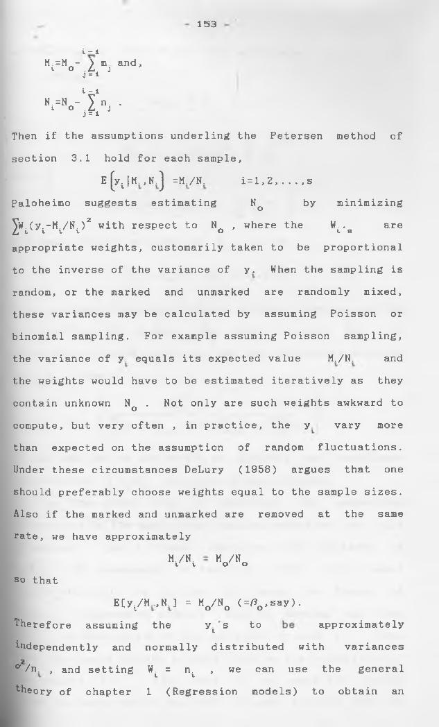
153

i - lM. =M - ) m and,1 ° j h '

i - 1N. =N - y n. .t o .Li JJ = l

Then if the assumptions underling the Petersen method of

section 3.1 hold for each sample,

E(yi|H.,N.) =M./N. i=l, 2, . . . , s

Paloheimo suggests estimating Nq by minimizing

Yw. (y.-M./N. )2 with respect to N , where the W. , are£ V V t t O t sappropriate weights, customarily taken to be proportional

to the inverse of the variance of y. When the sampling is

random, or the marked and unmarked are randomly mixed,

these variances may be calculated by assuming Poisson or

binomial sampling. For example assuming Poisson sampling,

the variance of y equals its expected value M./IT and

the weights would have to be estimated iteratively as they

contain unknown Nq . Not only are such weights awkward to

compute, but very often , in practice, the y vary more

than expected on the assumption of random fluctuations.

Under these circumstances DeLury (1958) argues that one

should preferably choose weights equal to the sample sizes.

Also if the marked and unmarked are removed at the same

rate, we have approximately

so thatM./N.V t Mc/No

E[y/M.,N.] = Mo/No <=^0 ,Say).

Therefore assuming the yt s to approximatelyindependently and normally distributed with variances

° /rr , and setting W = n , we can use the general

theory of chapter 1 (Regression models) to obtain an

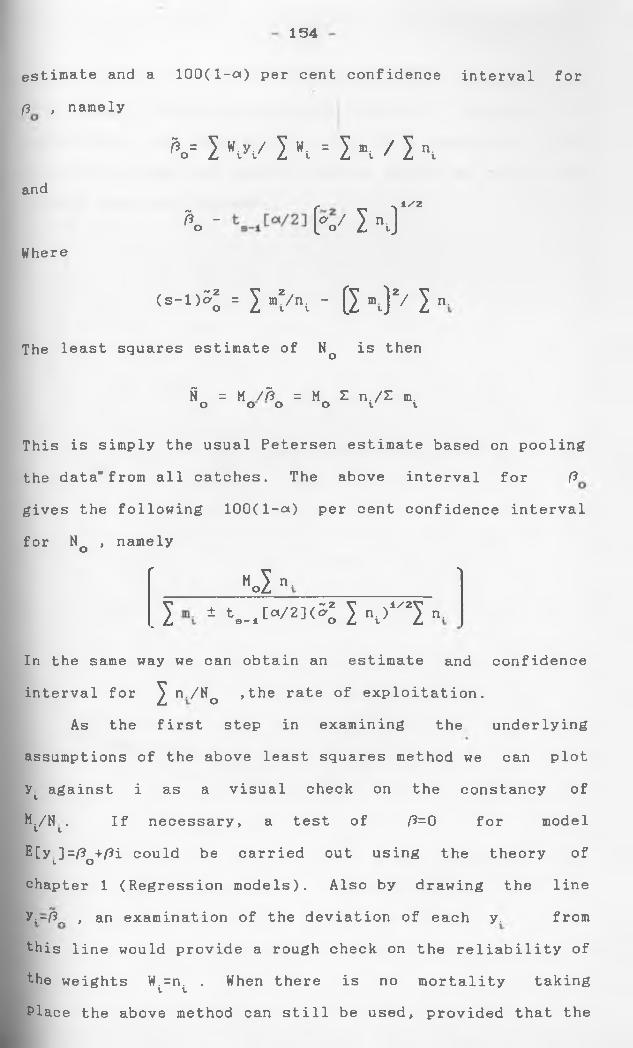
154

estimate and a 100(l-o<) per cent confidence interval for

ft , namely

K= 1 w H = K / Kand

K - { % / 1 " J 1"2Where

( S- 1 ) ^ = £ < / " , - g mt) 2/ J n.

The least squares estimate of Nq is then

fi = M /ft = M Z n./Z m.O O O O l V

This is simply the usual Petersen estimate based on pooling

the data*from all catches. The above interval for ft gives the following lOO(l-ot) per cent confidence interval

for Nq , namely

[ H j n .__________________ '

. I 4 t 8- 1[ « / 2] ( ^ l n S ' 2l n.

In the same way we can obtain an estimate and confidence

interval for ^ n./No >the rate of exploitation.

As the first step in examining the underlying

assumptions of the above least squares method we can plot

yt against i as a visual check on the constancy of

Ml/Nl. If necessary, a test of ft=0 for model

E[yil=^o+/?i could be carried out using the theory of

chapter 1 (Regression models). Also by drawing the line

^i-ft* > an examination of the deviation of each y. from

this line would provide a rough check on the reliability of

the weights W.=n. . When there is no mortality takingt tPlace the above method can still be used, provided that the

155

mortality rates for marked and unmarked are the same, so

that M/N remains approximately constant. However, if

recruitment and immigration into the population are

appreciable then more complex methods which we shall not

discuss here are required.

CHAPTER 44.1 SCHNABEL CENSUS.Notation.

A simple extension of the Petersen method to a series

of s samples of sizes n . no .... . n is the so called* Z SSchnabel census (Schnabe1,1938). In this method each

sample captured (except the first) is examined for marked

members and then every member of the sample is given

another mark before the sample is returned to the

population. If different marks or tags are used for

different samples, then capture-recapture history of any

animal caught is known. For the closed population, a

variety of theoretical models have been suggested, but

before we discuss these, we shall need the following

notation:

N =total population size,

s =number of samples

nt =size of the ith sample (i=l, 2 s)

m. = number of marked individuals in ntu. = n.-m.t t v

Since there we have ir 0 as, the total the end of

different

hT= E mj » i 1,2,.... s + 1

= number of marked individuals in the

population just before the ith sample is

taken

are no marked animals in the first sample,

, M =0 , M =u =u and define M , (=r,say)

number of marked animals in the population at

the experiment that is, the total number

animals caught throughout the experiment.

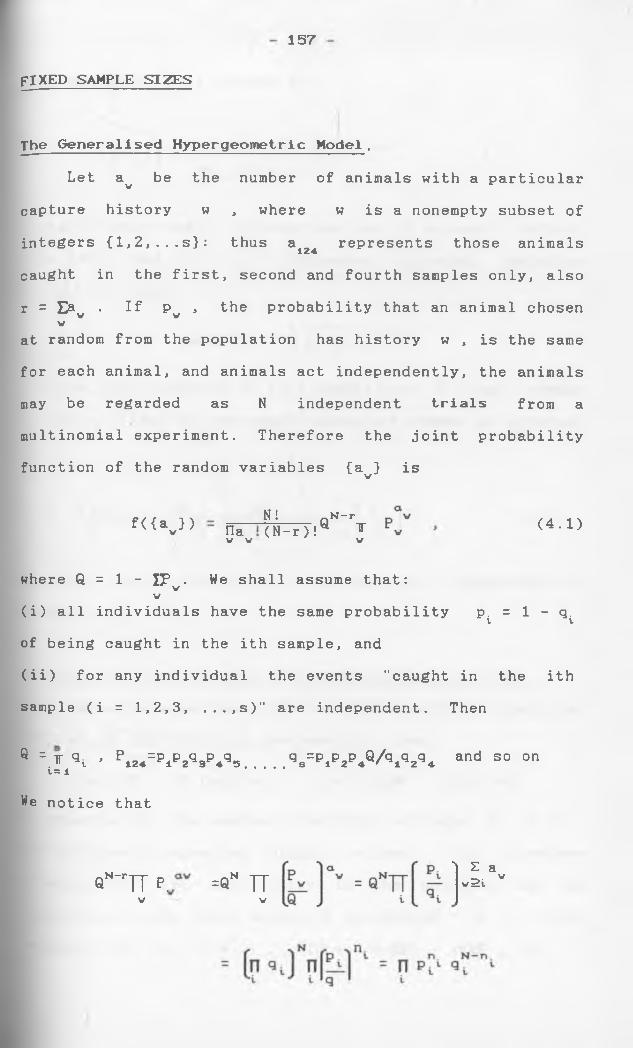
157

FIXED SAMPLE SIZES

The Generalised Hypergeometric Model.

Let av be the number of animals with a particular

capture history w , where w is a nonempty subset of

integers {l,2,...s}: thus * tZ4r represents those animals

caught in the first, second and fourth samples only, also

r = £&v • If Pv , the probability that an animal chosenV

at random from the population has history w , is the same

for each animal, and animals act independently, the animals

may be regarded as N independent trials from a

multinomial experiment. Therefore the joint probability

function of the random variables (a } isV

f<{av}) nav vN!(N-r)J Q

N-rTw

(4.1)

where Q = 1 - JP . We shall assume that:VV

(i) all individuals have the same probability p. = 1 - q.1 Vof being caught in the ith sample, and

(ii) for any individual the events "caught in the ith

sample (i = 1,2,3, ...,s)" are independent. Then

9 = T <3, . P124 = Pi P 2<33P «<35 q s =P lP2P4Q/ q i q 2q « an d 3 0 ° ni= l

We notice that

QN-rTT p, =eN TT' z

v 2 i

aVV V

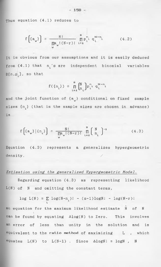
Thus equation (4.1) reduces to

f N!naw!(N-r)!

nn p ^i=l

N-nQ . »■ (4.2)

It is obvious from our assumptions and it is easily deduced

from (4.1) that n^s are independent binomial variables

B[n,p ], so that

f({n.}) ni=ln N — np.v q . v v t

and the joint function of {a^} conditional on fixed sample

sizes {n^} (that is the sample sizes are chosen in advance)

is

f K } l { n i>) = n . H H - r ) ! , n [ ” ) -1 ( 4 - 3 )1 1 V 1 = 1 VV

Equation (4.3) represents a generalizes hypergeometric

density. /

Estimation u s i n g the g e n e r a l i z e d H y p e r g e o m e t r i c Model.

Regarding equation (4.3) as representing likelihood

L(N) of N and omitting the constant terms,

log L(N) = E log(N-n.)i - (s-l)logN! - log(N-r)!i

an equation for the maximum likelihood estimate N of Ni

can be found by equating Alog(N) to Zero. This involves

an error of less than unity in the solution and is

equivalent to the ratio method of maximizing L , which

equates L(N) to L(N-l) . Since AlogN! = logN , N

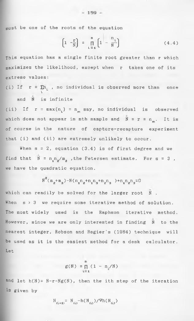
159

must be one of the roots of the equation

s r n . (■ - a * ni = i ( • - r )

This equation has a single finite root greater than

maximizes the likelihood, except when r takes one

extreme values:

(4.4)

r which

of its

(i) If r = , no individual is observed more than oncei

and N is infinite

(ii) If r = max{n.) = n say, no individual is observedv mwhich does not appear in mth sample and N = r = n . It ismof course in the nature of capture-recapture experiment

that (i) and (ii) are extremely unlikely to occur.

When s = 2, equation (3.4) is of first degree and we

find that N = ninz/m2 ,the Petersen estimate. For s = 3 ,

we have the quadratic equation.

N 0n2+m3)-N(nln2+nln3+n2n3 J + n ^ n ^ O

which can readily be solved for the larger root N .

When s > 3 we require some iterative method of solution.

The most widely used is the Raphson iterative method.

However, since we are only interested in finding N to the

nearest integer, Robson and Regier's (1964) technique will

be used as it is the easiest method for a desk calculator. Let

g(N) = n (1 - n./N)i— 1and let h(N)= N-r-Ng(N), then the ith step of the iteration

is given by

■ W H<i>"h<H(i>>/7h(H<i>>

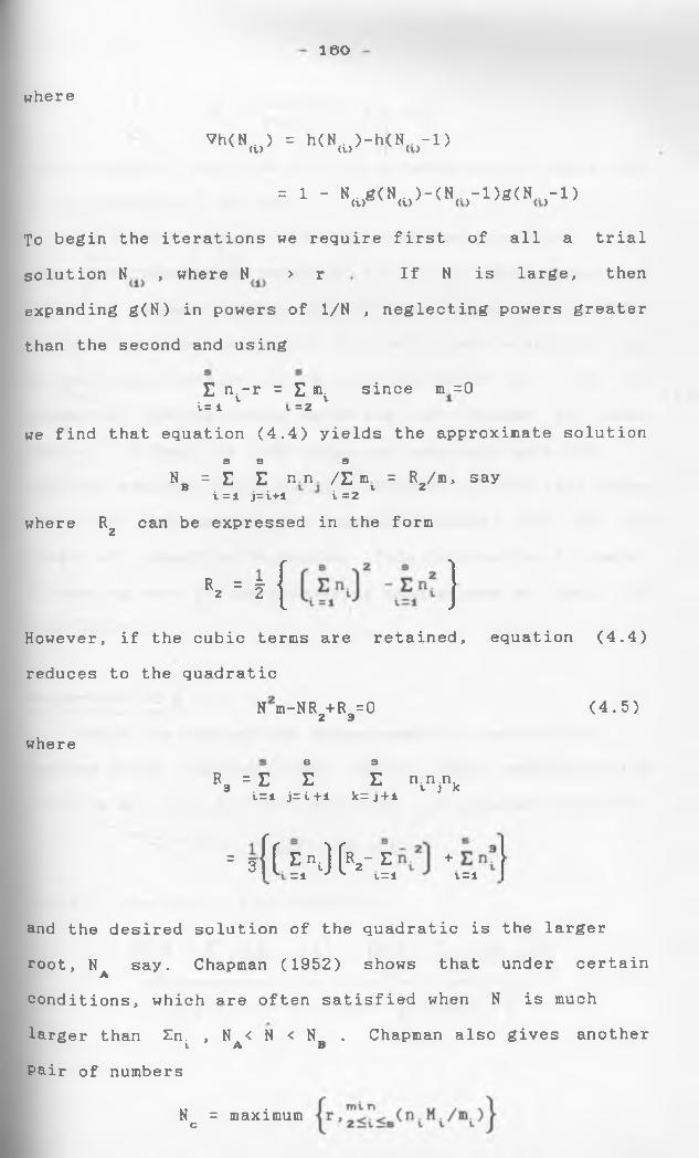
160

where

Vh(N(i)> = h(N(U)-h(N<.>-l)

= 1 - N(i,a(N<l,)-<H(.>-1)g(N<.,-1)

solution N , where N > r

To begin the iterations we require first of all a trial

If N is large, then

expanding g(N) in powers of 1/N , neglecting powers greater

than the second and using

E n.-r = E m.. t tt= 1 1=2since m =0

we find that equation (4.4) yields the approximate solutions s s

Nb = E E n.n /E mi = R2/m, sayi = 1 j= i+1 i=2

where Rz can be expressed in the form

r2 = f* { }

However, if the cubic terms are retained, equation (4.4)

reduces to the quadratic

N m-NR +R =02 3 (4.5)

wheresE

sER = E E E n.n.n,3 v j kL=1 j=i+l k=j+l

= sf( S nj ( v E +=1 J v 1=1 V=1

and the desired solution of the quadratic is the larger

root, N say. Chapman (1952) shows that under certainAconditions, which are often satisfied when N is much

larger than Zn. , N < N < N . Chapman also gives anotherl A BPair of numbers

N = maximumc

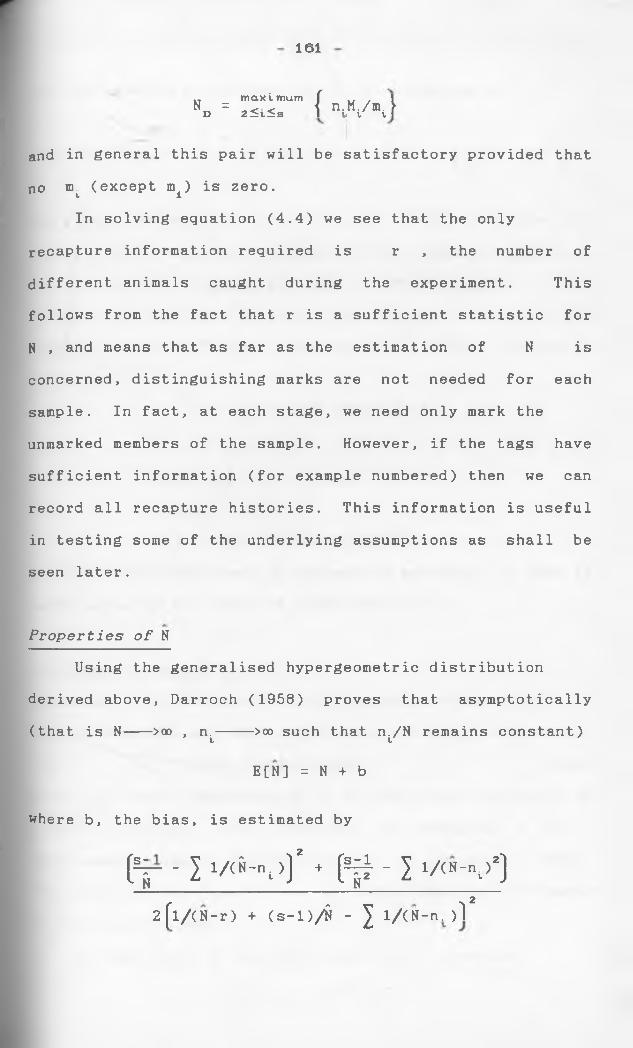
161

„ m a x im u m f .. . |N = 0< < < n.M./m. 1D 25i5s 1 ij v vl

and in general this pair will be satisfactory provided that

no mL (except mi) is zero.

In solving equation (4.4) we see that the only

recapture information required is r , the number of

different animals caught during the experiment. This

follows from the fact that r is a sufficient statistic for

N , and means that as far as the estimation of N is

concerned, distinguishing marks are not needed for each

sample. In fact, at each stage, we need only mark the

unmarked members of the sample. However, if the tags have

sufficient information (for example numbered) then we can

record all recapture histories. This information is useful

in testing some of the underlying assumptions as shall be

seen later.

P r o p e r t i e s o f N

Using the generalised hypergeometric distribution

derived above, Darroch (1958) proves that asymptotically

(that is N--->oo , n.---- >co such that n./N remains constant)t V

E[N] = N + b

, the bias, is estimated by

f j f - I I / C K ) ) 2 + ( ^ - - l l/(H-nt>2)

r -v22 |l/(N-r) + <s-l)/fi - J l/(N-n.)l

where b

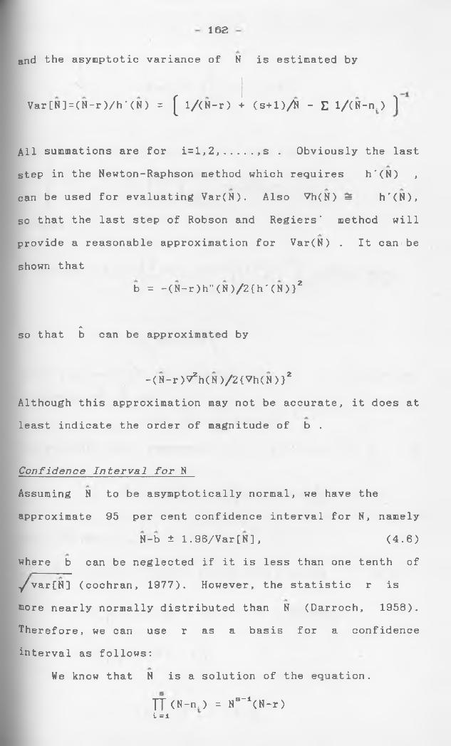
162

and the asymptotic variance of N is estimated by

Var[N]=(N-r)/h'(N) = £ l/(N-r) + (s+l)/K - £ l/(N-n.) 1

All summations are for i=l,2,.... ,s . Obviously the last

step in the Newton-Raphson method which requires h'(N) ,

can be used for evaluating Var(N). Also Vh(N) = h'(N),

so that the last step of Robson and Regiers' method will

provide a reasonable approximation for Var(N) . It can be

shown that

b = -<N-r)h"(N)/2{h'(N)}2

Aso that b can be approximated by

-(N-r)Vzh(N)/2{7h(N)}2

Although this approximation may not be accurate, it does at

least indicate the order of magnitude of b .

Confidence Interval for N

Assuming N to be asymptotically normal, we have the

approximate 95 per cent confidence interval for N, namely

N-b ± 1.96/Var[N], (4.6)

where b can be neglected if it is less than one tenth of

y/var[N] (cochran, 1977). However, the statistic r is

more nearly normally distributed than N (Darroch, 1958).

Therefore, we can use r as a basis for a confidence

interval as follows:

We know that N is a solution of the equation.

TT <N-n.) = Ns~‘(H-r)i = 1

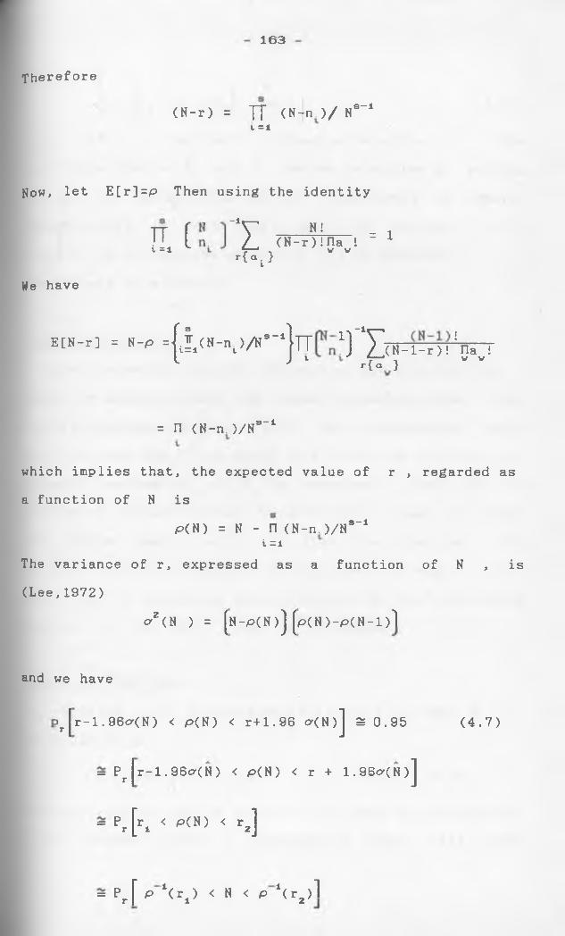
163

Therefore

(N-r) = JT (N-n.)/ N8 - 1

l =1

Now, let E[r]=p Then using the identity

-iiU . ( l } I n r / H

r{at }na !V V

= 1

We have

E[N-r] = N-p =(.[ j i ( H-nt ) / N - ‘ ITT X) ' X ( H - l - r ) ! ! 1 J 1 r {a }

na 1V V

= n (N-n. )/Ns-l

which implies that, the expected value of r , regarded as

a function of N is

p(N) = N - n (N-n. )/Ns —1i =1

The variance of r, expressed as a function of N , is

(Lee,1972)

o 2(N ) = (n -p (N)J [p(N)-p(N-l)l

and we have

>r |r-1 .96cr (N) < p(N) < r + 1 . 9 6 <?(N)J ^ 0 . 9 5

= Pr |r-1 .96o*(N) < p( N) < r + 1 . 96 o ' (N) J

= Pr[^ < P<M> < *,]

(4.7)

= Pr[ P 1(rl) < N < P ‘(r2)l

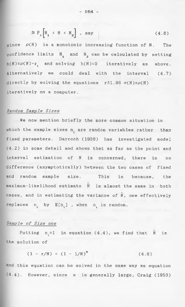
164

< N < (4.8)

since P(N) is a monotonic increasing function of N. The

confidence limits and Nz can be calculated by setting

h(N)=P(N)-ri and solving h(N)=0 iteratively as above.

Alternatively we could deal with the interval (4.7)

directly by solving the equations r±1.96 <?(N)=p(N)

iteratively on a computer.

Random S a m p l e S i z e s

We now mention briefly the more common situation in

which the sample sizes rv are random variables rather than

fixed parameters. Darroch (1958) has investigated model

(4.2) in some detail and shows that as far as the point and

interval estimation of N is concerned, there is no

difference (asymptotically) between the two cases of fixed

and random sample size. This is because, theA

maximum-likelihood estimate N is almost the same in both

cases, and in estimating the variance of N, one effectively

replaces n by E[n^] , when n is random.

Sample of Size one

Putting nL=l in equation (4.4), we find that N is

the solution of

(1 - r/N) = (1 - 1/N )s (4.9)

and this equation can be solved in the same way as equation

(4.4). However, since s is generally large, Craig (1953)

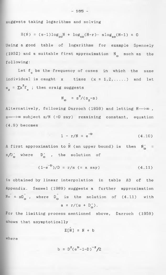
165

suggests taking logarithms and solving

H(N) = (s-l)logiQN + logio(N-r)- slogio(N-l) = 0

Using a good table of logarithms for example Spencely

(1952) and a suitable first approximation Nq such as the

following:

Let f be the frequency of cases in which the same

individual is caught x times (x = 1,2,.... ) and let2s2 = Ex fx ; then craig suggests

No = s 2/( s 2-s )

Alternatively, following Darroch (1958) and letting N— >oo ,

s--->oo subject s/N (=D say) remaining constant, equation

(4.9) becomes

1 - r/N = e ° (4.10)a

A first approximation to N (an upper bound) is then NT =

s/D' where D' , the solution of ' o o

( 1-e °)/D = r/s (= a say) (4.11)

is obtained by linear interpolation in table A3 of the

Appendix. Samwel (1969) suggests a further approximation

No = sD , where D is the solution of (4.11) with o oa = r/(s + D^).

For the limiting process mentioned above, Darroch (1959)

shows that asymptotically

E[N] = N + b

where

b = D2(eD-l-D) 2/2

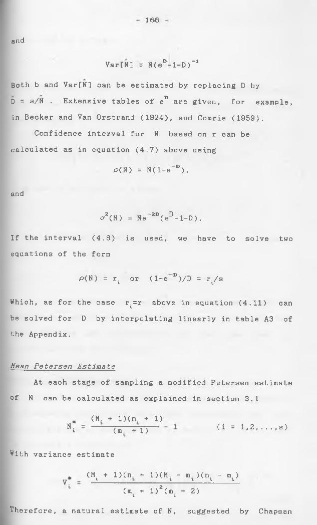
166

and

Var[N] = N(eD-l-D)'*

Both b and Var[N] can be estimated by replacing D by

D = s/N . Extensive tables of e° are given, for example,

in Becker and Van Orstrand (1924), and Comrie (1959).

Confidence interval for N based on r can be

calculated as in equation (4.7) above using

P(N) = N(l-e-D).

and

p2(N) = Ne_2D(eD-l-D).

If the interval (4.8) is used, we have to solve two

equations of the form

P(N) = rt or (1-e d)/D = r^/s

Which, as for the case r^=r above in equation (4.11) can

be solved for D by interpolating linearly in table A3 of the Appendix.

Mean P e t e r s e n E s t i m a t e

At each stage of sampling a modified

of N can be calculated as explained in

*N.i(M. + l)(n. + 1)

Cm"™+T)

Petersen estimate section 3.1

(i = 1,2,...,s)

With variance estimate

(M + 1)(n + 1 )(M - m )(n. - m.)1 V V v V(mi + l)2(mi + 2)

Therefore, a natural estimate of N, suggested by Chapman

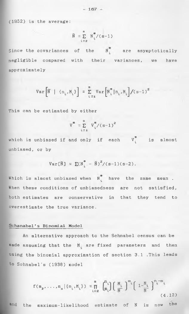
167

(1952) is the average:

sN = E N./<s-l)

1 = 2

Since the covariances of the N are asymptotically

negligible compared with their variances, we have

approximately

{n.,M.}] = Z_iVar[N*|n.,M.]/<s-l):

This can be estimated by either

sV = E Vt/(s-l)2

i = 1

*which is unbiased if and only if each V. is almostiunbiased, or by

Var[N] = E(N* - N )2/( s-1) (s-2) .

Which is almost unbiased when N. have the same mean .iWhen these conditions of unbiasedness are not satisfied,

both estimates are conservative in that they tend to

overestimate the true variance.

Schanabel*s Binomial ModelAn alternative approach to the Schnabel census can be

made assuming that the are fixed parameters and then

using the binomial approximation of section 3.1 .This leads

to Schnabel's (1938) model

f(m2,...,ms|{n.,M.}) l( i-jji) 1

(4.12)

ar>d the maximum-likelihood estimate of N is now the

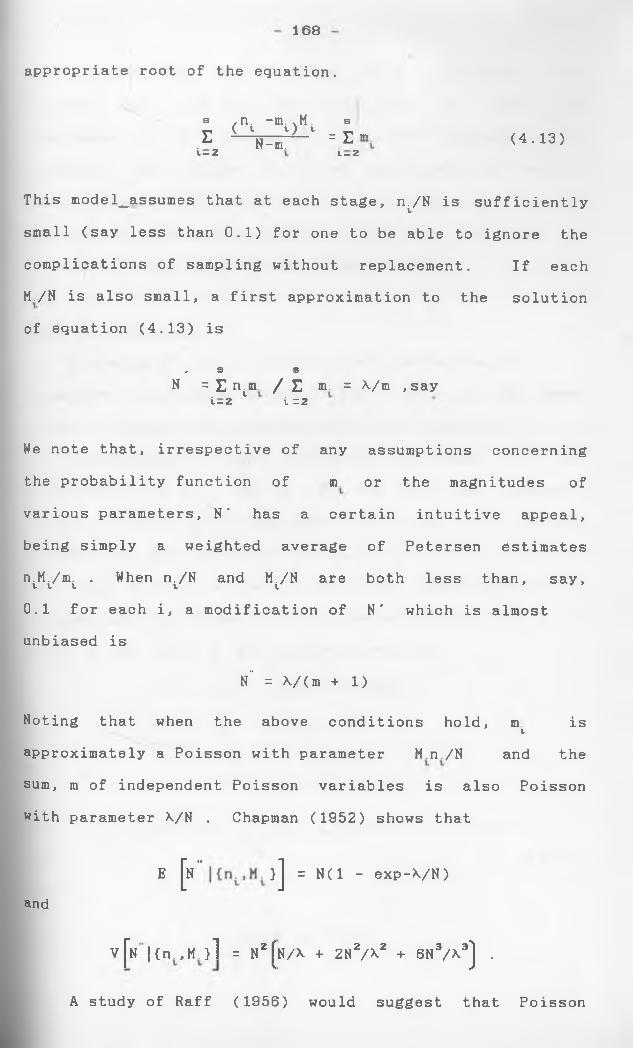
168

appropriate root of the equation.

s ,n. -m. XM . s r ( v O * - -r m E N-m. - i — 2 L —2(4.13)

This model^assumes that at each stage, nyN is sufficiently

small (say less than 0.1) for one to be able to ignore the

complications of sampling without replacement. If each

M./N is also small, a first approximation to the solution

of equation (4.13) is

, s sN = £ n nr / £ nr = X/m ,say

i — 2 i = 2

We note that, irrespective of any assumptions concerning

the probability function of nr or the magnitudes of

various parameters, N' has a certain intuitive appeal,

being simply a weighted average of Petersen estimatesn.M./m. . Whent V V n./N

Vand M./N are

Vboth less than, say,

0.1 for each i, a modification of N' which is almostunbiased is

N" = X/(m + 1)

Noting that when the above conditions hold, m isVapproximately a Poisson with parameter M.n./N and the

sum, m of independent Poisson variables is also Poisson

with parameter X/N . Chapman (1952) shows that

E [h " }] = N( 1 - exp-X/N)and

v [n |{n.,H.}l = H2[n/X + 2NZ/X2 + 6N3A 3] .

A study of Raff (1956) would suggest that Poisson

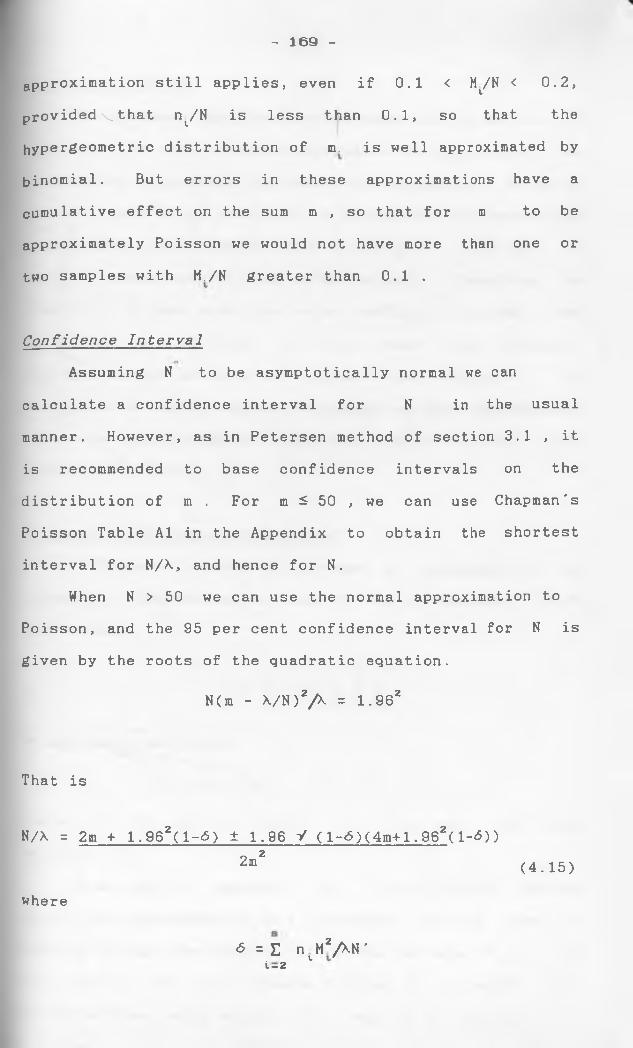
approximation still applies, even if 0.1 < M /N < 0.2,

provided v that nL/N is less than 0.1, so that the

- 169 -

hypergeometric distribution of nr is well approximated by

binomial. But errors in these approximations have a

cumulative effect on the sum m , so that for m to be

approximately Poisson we would not have more than one or

two samples with M./N greater than 0.1 .

Con f i d e n c e Interval

Assuming N to be asymptotically normal we can

calculate a confidence interval for N in the usual

manner. However, as in Petersen method of section 3.1 , it

is recommended to base confidence intervals on the

distribution of m . For m ^ 50 , we can use Chapman's

Poisson Table A1 in the Appendix to obtain the shortest

interval for N/X, and hence for N.

When N > 50 we can use the normal approximation to

Poisson, and the 95 per cent confidence interval for N is

given by the roots of the quadratic equation.

N(m - V N ) ZA = 1-962

That is

N/X = 2m + 1.962(l-6) ± 1.96 V (1-6)(4m+l.962( 1-6))2m2 (4.15)

<5 = £ n^M2/ M T 1 — 2

where

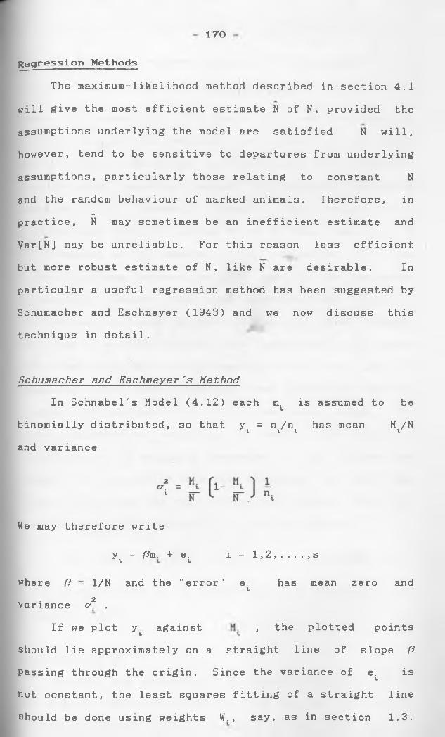
170

Regression MethodsThe maximum-likelihood method described in section 4.1

will give the most efficient estimate N of N, provided the

assumptions underlying the model are satisfied N will,

however, tend to be sensitive to departures from underlying

assumptions, particularly those relating to constant N

and the random behaviour of marked animals. Therefore, inA

practice, N may sometimes be an inefficient estimate and

Var[N] may be unreliable. For this reason less efficient

but more robust estimate of N, like N are desirable. In

particular a useful regression method has been suggested by

Schumacher and Eschmeyer (1943) and we now discuss this

technique in detail.

S c h u m a c h e r a nd E s c h m e y e r 's M e t h o d

In Schnabel's Model (4.12) each m. is assumed to betbinomially distributed, so that y. = m./n. has mean M./N

l V V V

and variance

We may therefore write

y i = fthl + el i=l,2,....,s

where ft - 1/N and the "error" eL has mean zero and 2variance o. .

If we plot y against , the plotted points

should lie approximately on a straight line of slope ft Passing through the origin. Since the variance of ei is

not constant, the least squares fitting of a straight line

should be done using weights VT, say, as in section 1.3.

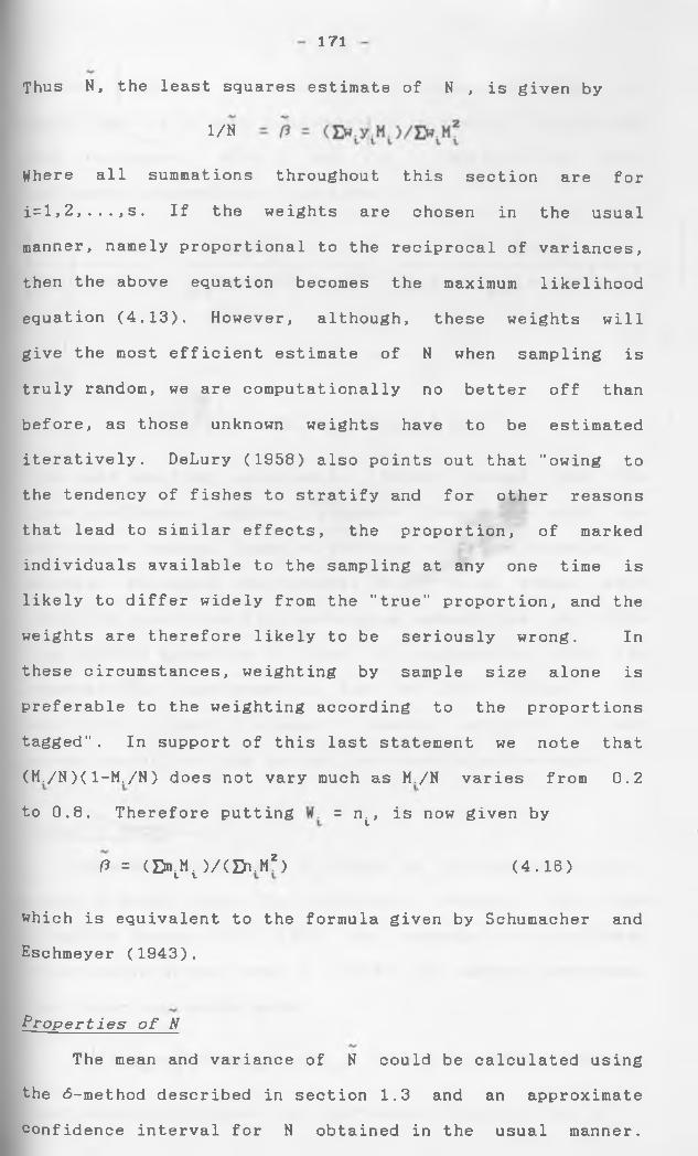
171

Thus N, the least squares estimate of N , is given by

l/N - ft -

Where all summations throughout this section are for

i=l,2,...,s. If the weights are chosen in the usual

manner, namely proportional to the reciprocal of variances,

then the above equation becomes the maximum likelihood

equation (4.13). However, although, these weights will

give the most efficient estimate of N when sampling is

truly random, we are computationally no better off than

before, as those unknown weights have to be estimated

iteratively. DeLury (1958) also points out that “owing to

the tendency of fishes to stratify and for other reasons

that lead to similar effects, the proportion, of marked

individuals available to the sampling at any one time is

likely to differ widely from the "true" proportion, and the

weights are therefore likely to be seriously wrong. In

these circumstances, weighting by sample size alone is

preferable to the weighting according to the proportions

tagged”. In support of this last statement we note that

(M./N)( 1-hT/N) does not vary much as ht/N varies from 0.2 to 0.8. Therefore putting = nt, is now given by

ft = ( B n ^ V C D v M * ) (4.16)

which is equivalent to the formula given by Schumacher and

Eschmeyer (1943).

P r o p e r t i e s o f N

The mean and variance of N could be calculated using

the <5-method described in section 1.3 and an approximate

confidence interval for N obtained in the usual manner.

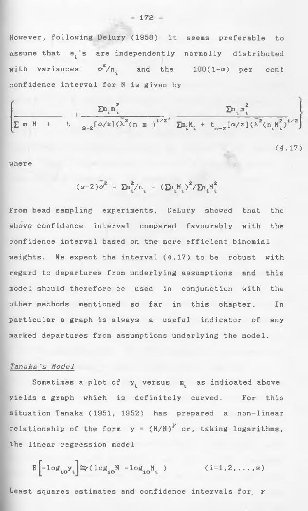
172

However, following Delury (1958) it seems preferable to

assume that et s are independently normally distributed

with variances o^/n^ and the lOO(l-ot) per cent

confidence interval for N is given by

£ m M + t

_ 2£m. m.it_ 2 Tm. m .

V t

[a/2](\z(n m )1/2S —2 Dn,M. + fc. ,t“/2K^(n.H*)t t s —z t t

where(4

(s-2)a = BnZ/rv - (BvM. )Z/Bi.MZ

From bead sampling experiments, DeLury showed that the%above confidence interval compared favourably with the

confidence interval based on the more efficient binomial

weights. We expect the interval (4.17) to be robust with

regard to departures from underlying assumptions and this

model should therefore be used in conjunction with the

other methods mentioned so far in this chapter. In

particular a graph is always a useful indicator of any

marked departures from assumptions underlying the model.

Tanaka's Model

Sometimes a plot of y. versus m as indicated abovet tyields a graph which is definitely curved. For this

situation Tanaka (1951, 1952) has prepared a non-linearVrelationship of the form y = (M/N) or, taking logarithms,

the linear regression model

, E[-logloy.]^(logloN -logloM. ) ( i=l, 2, . . . , s)

Least squares estimates and confidence intervals for Y

1/2

.17)

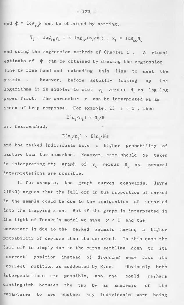
173

and <J> = lo^10N can be obtained by setting.

Yi = l0giOyt = = 1°eio<ni/'ni> - *t = loeioMt

and using the regression methods of Chapter 1 . A visual

estimate of <|> can be obtained by drawing the regression

line by free hand and extending this line to meet the

x-axis . However, before actually looking up the

logarithms it is simpler to plot y versus M. on log-log

paper first. The parameter r can be interpreted as an

index of trap response. For example, if r < 1 , then

E[mi/ni] > M./Nor, rearranging,

E[m./n.] > E[n./N]

and the marked individuals have a higher probability of

capture than the unmarked. However, care should be taken

in interpreting the graph of y versus M. as several

interpretations are possible.

If for example, the graph curves downwards, Hayne

(1949) argues that the fall-off in the proportion of marked

in the sample could be due to the immigration of unmarked

into the trapping area. But if the graph is interpreted in

the light of Tanaka's model we have r < 1 and the

curvature is due to the marked animals having a higher

probability of capture than the unmarked. In this case the

fall off is simply due to the curve settling down to its

"correct" position instead of dropping away from its

"correct" position as suggested by Hyne. Obviously both

interpretations are possible, and one could perhaps

distinguish between the two by an analysis of the

recaptures to see whether any individuals were being

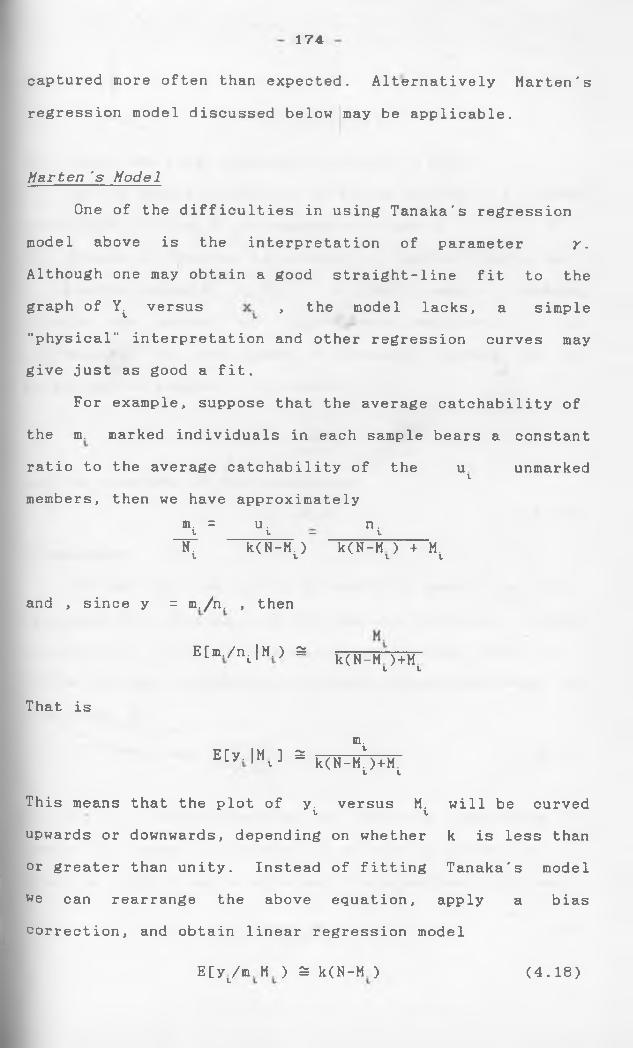
174

captured more often than expected. Alternatively Marten's

regression model discussed below may be applicable.

M a r t e n 's Model

One of the difficulties in using Tanaka's regression

model above is the interpretation of parameter y.

Although one may obtain a good straight-line fit to the

graph of Yt versus , the model lacks, a simple

"physical" interpretation and other regression curves may

give just as good a fit.

For example, suppose that the average catchability of

the nr marked individuals in each sample bears a constant

ratio to the average catchability of the u unmarked

members, then we have approximatelym. = u. n.t l — L

I T k(N-M. ) k(N-M ) + M.V l t t

and , since y = nr/rr , then

ECm./njM.) 2= k(H_H )+Mt L

That is

m.tk(N-M. )+M.t V

This means that the plot of y. versus M. will be curvedt i.upwards or downwards, depending on whether k is less than

or greater than unity. Instead of fitting Tanaka's model

we can rearrange the above equation, apply a bias

correction, and obtain linear regression model

E[y^/nr M. ) ^ k(N-M )

E[y.|Mt] ^

( 4 . 18)

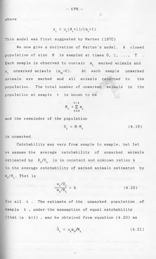
175

where

y. = u. (M. + l)/(m. + l)t 1 1 i

This model was first suggested by Marten (1970)

We now give a derivation of Marten's model. A closed

population of size N is sampled at times 0, 1, T

Each sample is observed to contain mt marked animals and

u unmarked animals (m =0). At each sample unmarked t oanimals are marked and all animals returned to the

population. The total number of unmarked animals in the

population at sample t is known to be

* t-i= = “i 1 = 0

and the remainder of the population

Ut = N-Mt (4.19)

is unmarked.

Catchability may vary from sample to sample, but let

us assume the average catchability of unmarked animals

estimated by U /Ut is in constant and unknown ration k

to the average catchability of marked animals estimated by

mt/M . That is

V « tV Ht

k (4.20)

for all t . The estimate of the unmarked population of

sample t , under the assumption of equal catchability

(that is k=l) , may be obtained from equation (4.20) as

U = u m /Mt t t/ t (4.21)

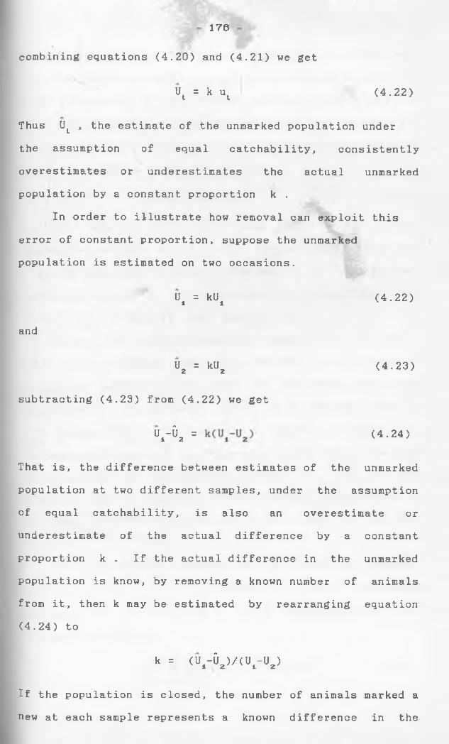
176

combining equations (4.20) and (4.21) we get

Ut = k ut (4.22)

Thus Ut , the estimate of the unmarked population under

the assumption of equal catchabi1ity, consistently

overestimates or underestimates the actual

population by a constant proportion k .unmarked

In order to illustrate how removal can exploit this

error of constant proportion, suppose the unmarked

population is estimated on two occasions.

ut = kUt

and

(4.22)

U = kU 2 2

subtracting (4.23) from (4.22) we get

(4.23)

V 6. = (4.24)

That is, the difference between estimates of the unmarked

population at two different samples, under the assumption

of equal catchability, is also an overestimate or

underestimate of the actual difference by a constant

proportion k . If the actual difference in the unmarked

population is know, by removing a known number of animals

from it, then k may be estimated by rearranging

(4.24) to

equation

k = (ur D2)/(ut-u2)

If the population is closed, the number of animals marked a

new at each sample represents a known difference in the

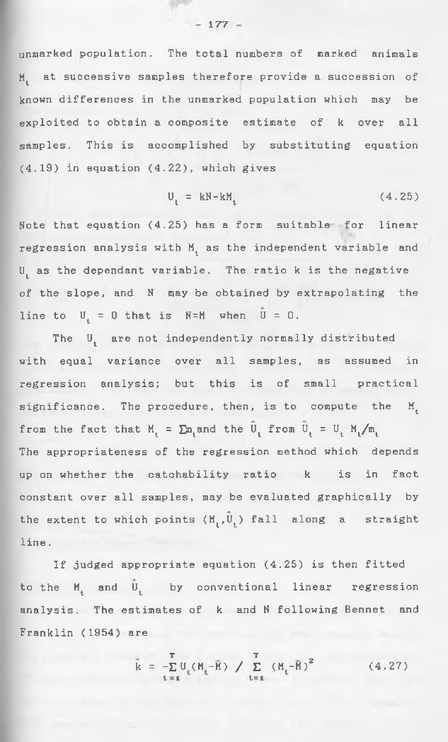
177

unmarked population. The total numbers of marked animals

Ht at successive samples therefore provide a succession of

known differences in the unmarked population which may be

exploited to obtain a composite estimate of k over all

samples. This is accomplished by substituting equation

(4.19) in equation (4.22), which gives

Ut = kN-kMt (4.25)

Note that equation (4.25) has a form suitable for linear

regression analysis with Mt as the independent variable and

Ut as the dependant variable. The ratio k is the negative

of the slope, and N may be obtained by extrapolating the

line to Ut = 0 that is N=M when U = 0.

The Ut are not independently normally distributed

with equal variance over all samples, as assumed in

regression analysis; but this is of small practical

significance. The procedure, then, is to compute the Mt

from the fact that Mt = £mtand the Ut from Ut = UL Ht/mt

The appropriateness of the regression method which depends

up on whether the catchability ratio k is in fact

constant over all samples, may be evaluated graphically byA

the extent to which points (Mt,Ut) fall along a straight

line.

If judged appropriate equation (4.25) is then fitted

to the Mt and Ut by conventional linear regression

analysis. The estimates of k and N following Bennet and

Franklin (1954) areT T

k = -EU.(H-M) / E (M -M)2 ( 4 . 27)

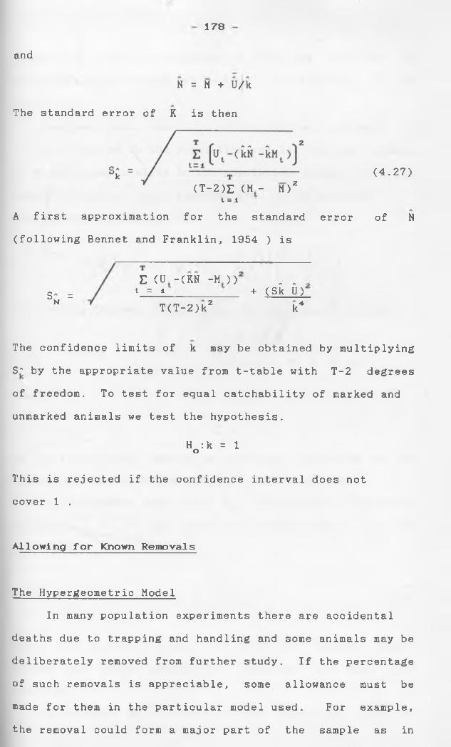
178

and

N = M + U/k

The standard error of K is then

(T-2)E <M - M)2t = 1

A first approximation for the standard error

(following Bennet and Franklin, 1954 ) is

(4.27)

of N

Sn =E (U -(KN -M )) . . .t = i__________ _ + (Sk U)

T(T-2)k2 k4

The confidence limits of k may be obtained by multiplying

S~ by the appropriate value from t-table with T-2 degrees

of freedom. To test for equal catchability of marked and

unmarked animals we test the hypothesis.

H :k = 1 o

This is rejected if the confidence interval does not

cover 1 .

A11owi ng f or Known Removals

The Hypergeometric Model

In many population experiments there are accidental

deaths due to trapping and handling and some animals may be

deliberately removed from further study. If the percentage

of such removals is appreciable, some allowance must be

made for them in the particular model used. For example,

the removal could form a major part of the sample as in

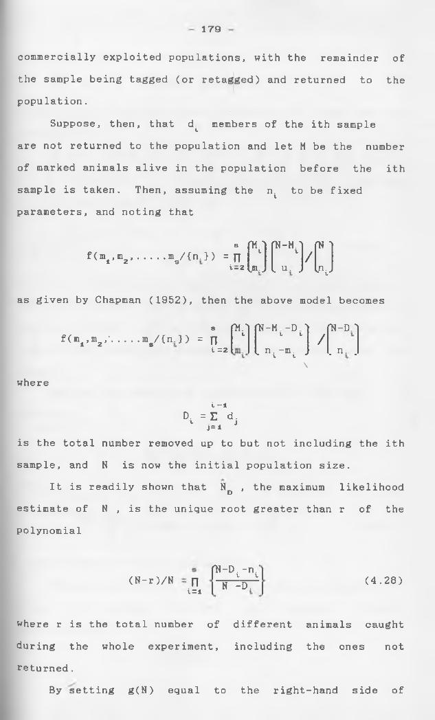
179

commercially exploited populations, with the remainder of

the sample being tagged (or retagged) and returned to the

population.

Suppose, then, that d members of the ith sample

are not returned to the population and let M be the number

of marked animals alive in the population before the ith

sample is taken. Then, assuming the nt to be fixed

parameters, and noting that

s fM 1 fN-M.l fN ]f <ml,m2,.... mg/{n. } ) = f] l V

/i-2 L J l u. J k J

as given by Chapman (1952), then the above model becomes

s r*n fN-H -D 1 fN-D "If(mi,m2,*. . . .ms/{n.}> = n

i =2X. V l.

. n.-m. „t y. */. n. .

\

where

i —1D. = E d. v j=i J

is the total number removed up to but not including the ith

sample, and N is now the initial population size.

It is readily shown that Nd , the maximum likelihood

estimate of N , is the unique root greater than r of the

polynomial

(N-r )/N : nt=i

fN-D. -n.‘l VN -D. (4.28)

where r is the total number of different animals caught

during the whole experiment, including the ones not

returned.

By setting g(N) equal to the right-hand side of

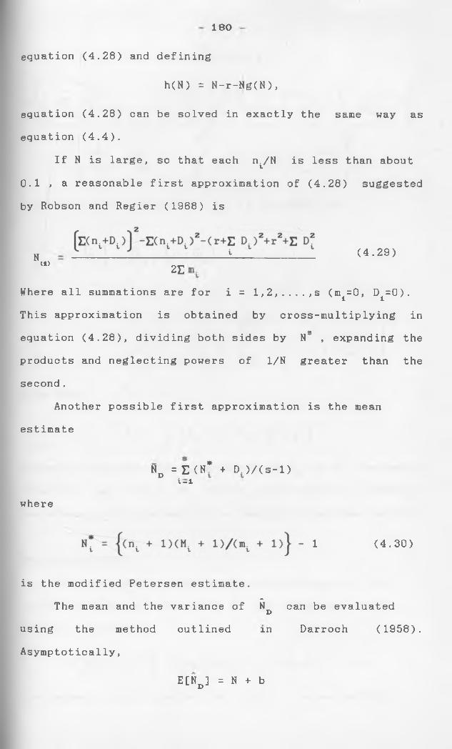
180

equation (4.28) and defining

h(N) = N-r-Ng(N),

equation (4.28) can be solved in exactly the same way as

equation (4.4).

If N is large, so that each r^/N is less than about

0.1 , a reasonable first approximation of (4.28) suggested

by Robson and Regier (1968) is

Where all summations are for i = l,2,....,s (mi=0, Di=0).

This approximation is obtained by cross-multiplying in

products and neglecting powers of 1/N greater than the

second.

Another possible first approximation is the mean

estimate

is the modified Petersen estimate.

The mean and the variance of & can be evaluatedD

N (4.29)< i >

2E

equation (4.28), dividing both sides by Ns , expanding the

Nd = £ (8* + D.)/(s-l)i-1

where

1 (4.30)

using the method outlined in Darroch (1958).

E[Nd] = N + b

Asymptotically,

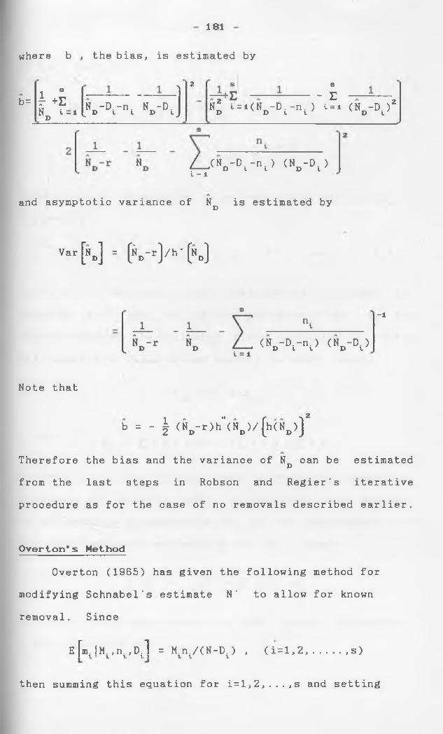
181

where b , the bias, is estimated by

1 8 b= r +EN t -1

D

— ------- — )V Dr"l «r>-D J

2 I s s- E

N* i = 1(Nn-D.-n. ) i = i (N -D. )2D D t v D t

H. Z _ ( V Dt-n i> < V Dt>i - 1

and asymptotic variance of Nd is estimated by

Var[«D] = («r,-r)/h '(«J

n.t-l

(N -D.-n. )D t l(N -D. )D l

Note that

b = - | (ND-r)h"(ND)/[h(ND)]

Therefore the bias and the variance of N can be estimatedD

from the last steps in Robson and Regier's iterative

procedure as for the case of no removals described earlier.

Overton* s Method

Overton (1965) has given the following method for

modifying Schnabel's estimate N' to allow for known

removal. Since

E [m. IM., n., D.l = M.n./(N-D.) , (i=l,2,.... ,s)t t t t I V t V

then summing this equation for i=l,2,...,s and setting

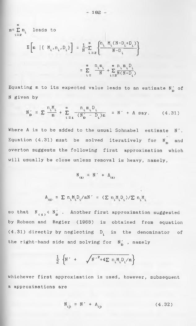
182

sm= E m leads toi—2

E [“ U = g-E*- J i =;fn. M. (N-D.+D. )

N-D

n.m. s n. m. D.1 * . r-. V t VN >N(N-D.)v=2 t

Equating m to its expected value leads to an estimate N' ofDN given by

n M s n . m . D .(HJ’ - D )mt = 1 D l '

= N' + A say. (4.31)

Where A is to be added to the usual Schnabel estimate N'.

Equation (4.31) must be solved iteratively for Nd and

overton suggests the following first approximation which

will usually be close unless removal is heavy, namely,

N< i > + A<„

A = E n.M.D./mN' = (E n.M.D.)/E n.M.

so that N < Nd . Another first approximation suggested

by Robson and Regier (1968) is obtained from equation

(4.31) directly by neglecting Dt in the denominator of

the right-hand side and solving for Nd , namely

| {iT + / n '2+4E n^D./m}

whichever first approximation is used, however, subsequent

a approximations are

<j> »' + A<j. (4.32)

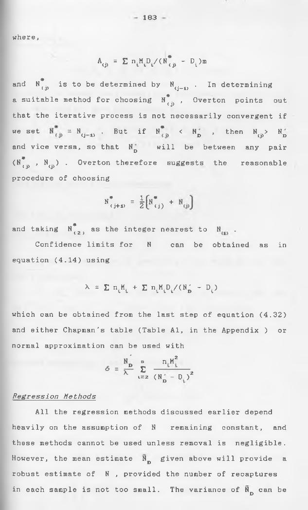
183

where,

A/ v = E n.M D /(N* - D. )m<J> t V t <J> l

*and N {j) is to be determined by N( _1) . In determining*a suitable method for choosing N { , Overton points out

that the iterative process is not necessarily convergent if

we set = N(j l) . But if N*., < ND , then N(j>> «D

and vice versa, so that Nd will be between any pair m(N<j> , N(j)) . Overton therefore suggests the reasonable

procedure of choosing

C . > = l [ < o +

*and taking N (z> as the integer nearest to N .

Confidence limits for N can be obtained as in

equation (4.14) using

X = £ n.M. + E n.M.D./(N' - D.)tt t t v D i

which

and e

norma

can be obtained from

ither Chapman's table

1 approximation can be

the last step of equation (4.32)

(Table Al, in the Appendix ) or

used with

s n.M2E -- — --1=2 <Nd - D.)2

R e g r e s s i o n M e t h o d s

All the regression methods discussed earlier depend

heavily on the assumption of N remaining constant, and

these methods cannot be used unless removal is negligible.

However, the mean estimate N given above will provide aDrobust estimate of N , provided the number of recaptures

in each sample is not too small. The variance of N can beD

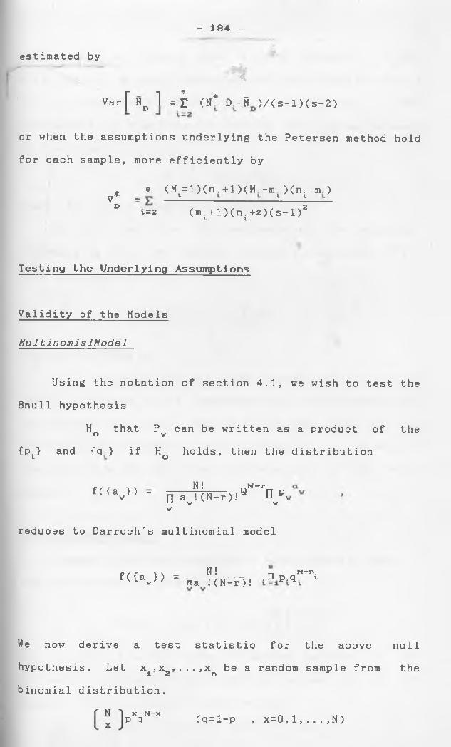
estimated by

- V " ^ ’ 1Var[ Nd 1 = £ (N*-D-fi )/(s-l)(s-2)

or when the assumptions underlying the Petersen method hold

for each sample, more efficiently by

* s (M. = 1 )(n .+1 )(M.-m )(n.-m.)y* _ *•_____ ^ iD i=2 (mi+l)(mi+2 )(s-l)2

Testing the Underlying Assumptions

Validity of the Models

Mu Itino m i a l M o d e l

- 184 -

Using the notation of section 4.1, we wish to test the

8null hypothesis

H that P can be written as a product of theO v{pt} and {q.} if Hq holds, then the distribution

N! LN-rf((av}) - n a i (N-r)!Q n p>

11 V VV

reduces to Darroch's multinomial model

N! N-n.f({a }) = -------- r, • n p.q iv J y rra i(N-r)!

We now derive a test statistic for the above null

hypothesis. Let x .x . ...,x be a random sample from the1 z nbinomial distribution.

x N-xp q (q=i-p , x=0,l,...,N)

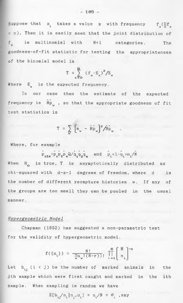
185

Suppose that x. takes a value x with frequency f (£f1 X X X= n), Then it is easily seen that the joint distribution of

f is multinomial with N+l categories. The

goodness-of-fit statistic for testing the appropriateness

of the binomial model is

T = V (f -E )2/EL x x ' xX — O

Where E^ is the expected frequency.

In our case then the estimate of the expected

frequency is Np^ , so that the appropriate goodness of fit

test statistics is

T == 1 ( a v - N P v jV & P ,

Where, for example

P124 = P,P2P4Q/^ ^ 2 and Pi=1-gi=n/K When Hq is true, T is asymptotically distributed as

chi-squared with d-s-1 degrees of freedom, where d is

the number of different recapture histories w. If any of

the groups are too small they can be pooled in the usual

manner.

H y p e r g e o m e t r i c Model

Chapman (1952) has suggested a non-parametric test

for the validity of hypergeometric model.

N!- na !(N_r))i i I V V V = 1

TT n .t

-l

Let b (i < j) be the number of marked animals in the

jth sample which were first caught and marked in the ith

sample. When sampling is random we have

E[b ,/n | n , u ] = u/N = 0 ,saywj V J o V t

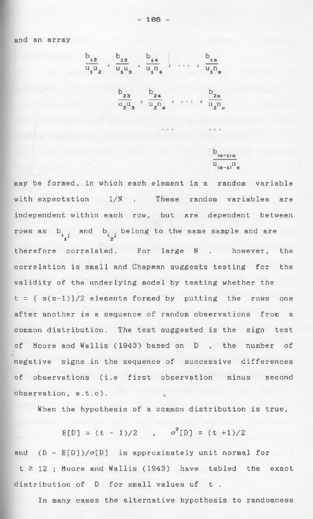
186

and an array

12

V 2

b b b13 1 4 I s

C e v* u n * ‘ • ' u nCT)'H 1 4 1 s

b b b2 3 2 4 2 s

u u u n2 3 2 4 u n2 s

(s-l>s (8-l>n s

may be formed, in which each element is a random variable

with expectation 1/N . These random variables are

independent within each row, but are dependent between

rows as b. . and b. . belong to the same sample and areV J t J1 2

therefore correlated. For large N . however, the

correlation is small and Chapman suggests testing for the

validity of the underlying model by testing whether the

t = { s(s-l)}/2 elements formed by putting the rows one

after another is a sequence of random observations from a

common distribution. The test suggested is the sign test

of Moore and Wallis (1943) based on D , the number of

negative signs in the sequence of successive differences

of observations (i.e first observation minus second

observation, e.t.c).

When the hypothesis of a common distribution is true,

E[D] = (t - 1 )/2 , o'2[D] = (t +l)/2

and (D - E[D])/o'[D] is approximately unit normal for

t £ 12 ; Moore and Wallis (1943) have tabled the exact

distribution of D for small values of t .

In many cases the alternative hypothesis to randomness

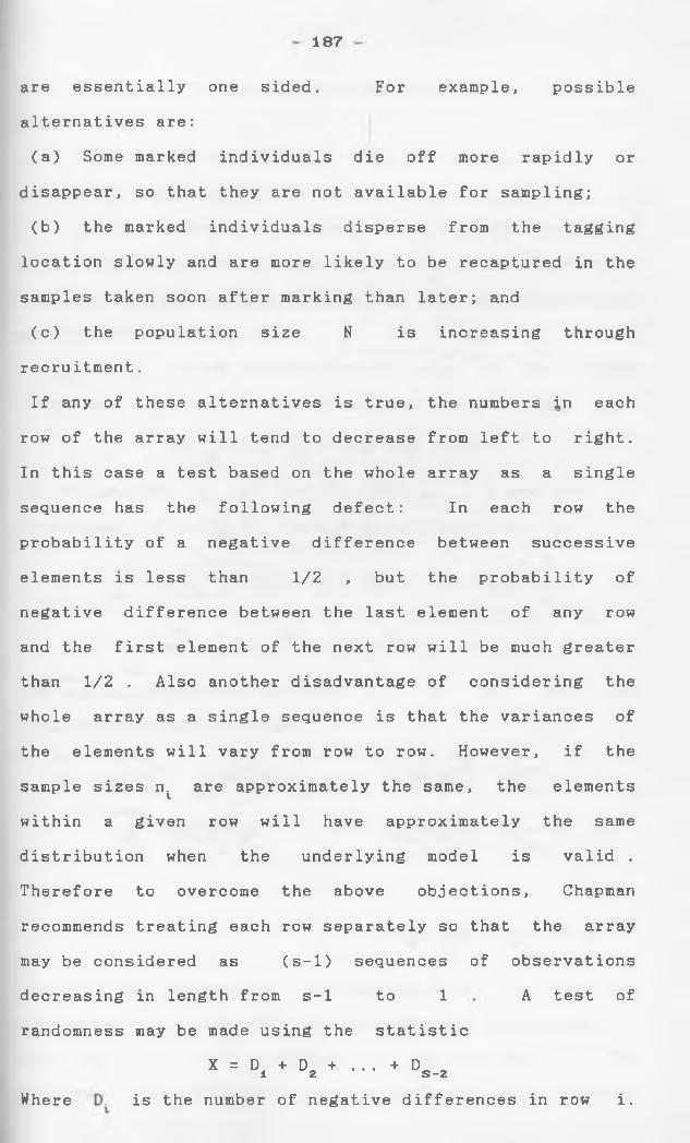
187

are essentially one sided. For example, possible

alternatives are:

(a) Some marked individuals die off more rapidly or

disappear, so that they are not available for sampling;

(b) the marked individuals disperse from the tagging

location slowly and are more likely to be recaptured in the

samples taken soon after marking than later; and

(c) the population size N is increasing through

recruitment.

If any of these alternatives is true, the numbers in each

row of the array will tend to decrease from left to right.

In this case a test based on the whole array as a single

sequence has the following defect: In each row the

probability of a negative difference between successive

elements is less than 1/2 , but the probability of

negative difference between the last element of any row

and the first element of the next row will be much greater

than 1/2 . Also another disadvantage of considering the

whole array as a single sequence is that the variances of

the elements will vary from row to row. However, if the

sample sizes nt are approximately the same, the elements

within a given row will have approximately the same

distribution when the underlying model is valid .

Therefore to overcome the above objections, Chapman

recommends treating each row separately so that the array

may be considered as (s-1) sequences of observations

decreasing in length from s-1 to 1 A test of

randomness may be made using the statistic

X = D + D + ... + D1 2 S —2Where is the number of negative differences in row i.

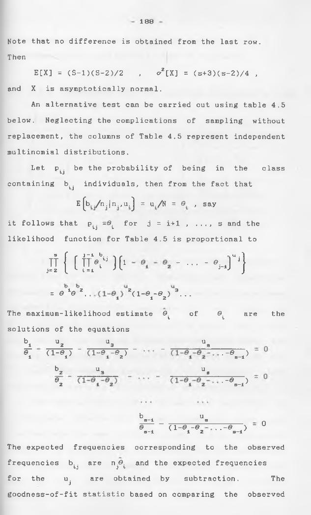
188

Note that no difference is obtained from the last row.

Then

E[X] = (S-l)(S-2)/2 , o-z[X] = (s+3)(s-2)/4 ,and X is asymptotically normal.

An alternative test can be carried out using table 4.5

below. Neglecting the complications of sampling without

replacement, the columns of Table 4.5 represent independent

multinomial distributions.

Let p^ be the probability of being in the class

containing b.. individuals, then from the fact thattjE(b../n.|n .,u.) = u./N = ©. , say

it follows that p.. -Q. for j = i+ 1 , ..., s and thetj Vlikelihood function for Table 4.5 is proportional to

j i { ( ! i ! ^ H * - - - v f 1 }

= e 40 2.. z(i-or e 2 ) 9...

The maximum-likelihood estimate 0 of 0. are theV l

solutions of the equations biWi

U 2 U 3 U sd - ^ )

11/~SN051051tH1

.-e ) "s-l

b 2 U 3 U s0 2 . - 0 ) " s-l'

1M1

• (0

-Q u8e (1-0 -0 ..-0 )s-l 1 2 s—1"

- 0

The expected frequencies corresponding to the observed

frequencies b.. are n .0. and the expected frequenciesUJ j V

for the u. are obtained by subtraction. Thejgoodness-of-fit statistic based on comparing the observed

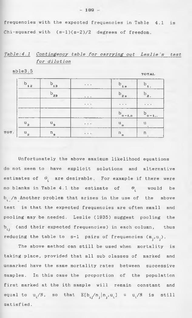
189

frequencies with the expected frequencies in Table 4.1 is

Chi-squared with (s-l)(s-2)/2 degrees of freedom.

T a b l e :4.1 C o n t i n g e n c y table for c a r r y i n g out L e s l i e ' s test for d i l u t i o n

able3.5---------------------- T O T A L

b1 2 b 13 . . . b ,3 b i.b,o b b23 . . . 2 s 2 .

. . .

b bs -l,s s -1,.uo U Q U U2 3 sU n^ n n2 3 s

Unfortunately the above maximum likelihood equations

do not seem to have explicit solutions and alternative

estimates of 9 are desirable. For example if there were

no blanks in Table 4.1 the estimate of 9. would betb i /n Another problem that arises in the use of the above

test is that the expected frequencies are often small and

pooling may be needed. Leslie (1935) suggest pooling the

b_ (and their expected frequencies) in each column, thus

reducing the table to s- 1 pairs of frequencies (nL,u^).

The above method can still be used when mortality is

taking place, provided that all sub classes of marked and

unmarked have the same mortality rates between successive

samples. In this case the proportion of the population

first marked at the ith sample will remain constant and

equal to u./N, so that E[b. ./n. |n.,u. ] = u./N is still VJ J J V Vsat isf ied.

190

R e g r e s s i o n Model

The best evidence for the validity of the Schumacher and Eschmeyer's regression method is obviously the linearity of the graph. Any change in N throughrecruitment, mortality, etcetera or any variation in catchability will affect the basic equation E[m /ni] = MVN and this in turn will show up in the graph provided the nr are not too small. In practice, point andinterval estimates of N should be obtained using as many different methods as possible, as any departures from underlying assumptions will usually affect differentmodels in different ways. A substantial agreement among the estimates would then give support for the validity of the models concerned.

Tests for R a ndom S a m p l i n g

A part from poor experimentation and inadequate experimental design, there are three basic sources of non-randomness:(a) There may be sub categories in the population due to size, sex, species, etcetera; for which sampling is random within each sub category, but not between the sub categories. In this case, if there is no mortality, the chi-squared goodness-of-fit test based on the following contingency table

SUBCATEOORY TOTALX Y • • • w

Recaptured m2 x m2y 2 w n 2Not recap. n -mlx 2x niy mzy . . . niv_m2vNo.releas. n1 X niy . . . "lv ni

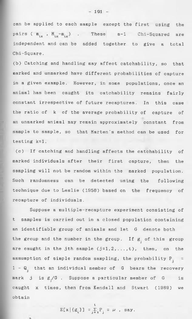
191

can be applied to each sample except the first using the

pairs ( mix , . These s-1 Chi-Squared are

independent and can be added together to give a total

Chi-Square.

(b) Catching and handling may affect catchability, so that

marked and unmarked have different probabilities of capture

in a given example. However, in some populations, once an

animal has been caught its catchability remains fairly

constant irrespective of future recaptures. In this case

the ratio of k of the average probability of capture of

an unmarked animal may remain approximately constant from

sample to sample, so that Marten's method can be used for

testing k=l.

(c) If catching and handling affects the catchability of

marked individuals after their first capture, then the

sampling will not be random within the marked population.

Such randomness can be detected using the following

technique due to Leslie (1958) based on the frequency of

recapture of individuals.

Suppose a multiple-recapture experiment consisting of

t samples is carried out in a closed population containing

an identifiable group of animals and let G denote both

the group and the number in the group. If gj of this group

are caught in the jth sample (j = 1 ,2 , . . . ,t) , then, on the

assumption of simple random sampling, the probability P =

1 - Qj that an individual member of G bears the recovery

mark j is g^/G • Suppose a particular member of G is

caught x times, then from Kendall and Stwart (1969) we

obtaint

E[x|{g }] = ? P = v , say.1 J — 1 J

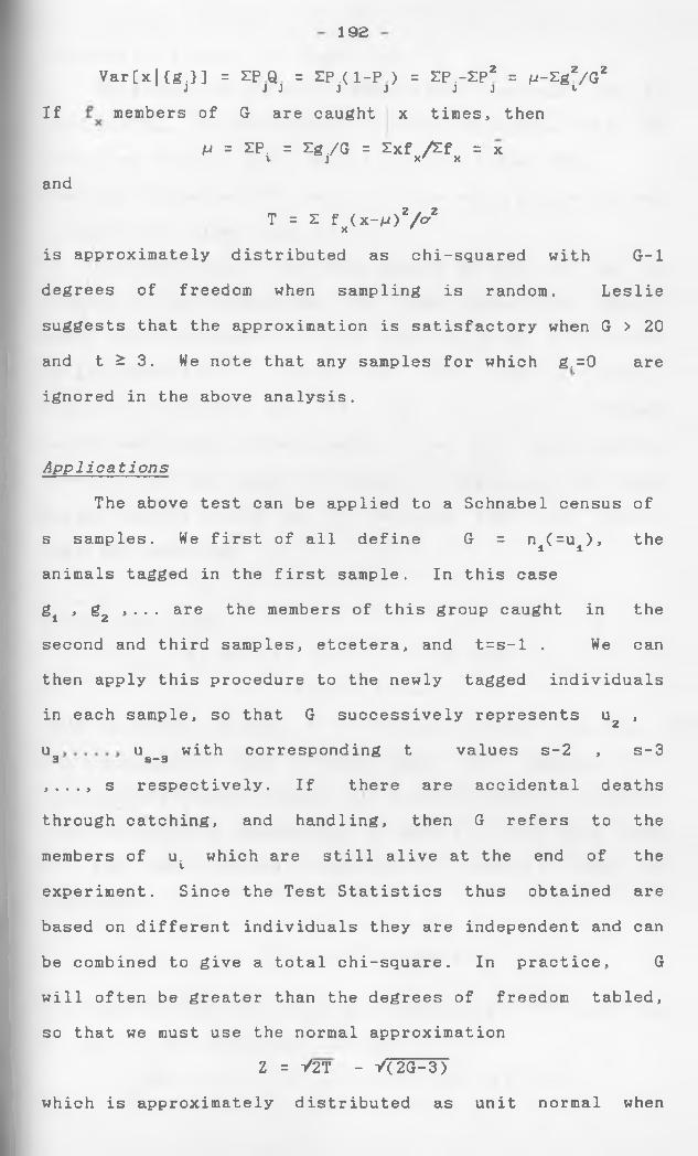
192

Var [x | {g.} ] = ZPQ = ZP.(l-P) = ZP.-ZP2 = p-Zgz/G2J J J J J J J ^If members of G are caught x times, then

M = ZP. = Zg./G = Zxf A f = xt J x' X

and

T = Z fx(x-/J)2/o2

is approximately distributed as chi-squared with G-l

degrees of freedom when sampling is random. Leslie

suggests that the approximation is satisfactory when G > 20

and t ^ 3. We note that any samples for which g.^0 are

ignored in the above analysis.

A p p l i c a t i o n s

The above test can be applied to a Schnabel census of

s samples. We first of all define G = ni(=ui), the

animals tagged in the first sample. In this case

g± , g2 , ... are the members of this group caught in the

second and third samples, etcetera, and t=s-l . We can

then apply this procedure to the newly tagged individuals

in each sample, so that G successively represents u2 ,

u u with3 S-3 corresponding t values s - 2 > s-3

,..., s respectively. If there are accidental deaths

through catching, and handling, then G refers to the

members of u. which are still alive at the endV of the

experiment. Since the Test Statistics thus obtained are

based on different individuals they are independent and can

be combined to give a total chi-square. In practice, G

will often be greater than the degrees of freedom tabled,

so that we must use the normal approximation

Z = -/2T - V( 2G-3)

which is approximately distributed as unit normal when

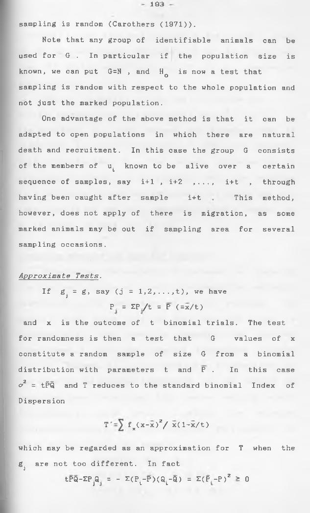
193

sampling is random (Carothers (1971)).

Note that any group of identifiable animals can be

used for G . In particular if the population size is

known, we can put G=N , and Hq is now a test that

sampling is random with respect to the whole population and

not just the marked population.

One advantage of the above method is that it can be

adapted to open populations in which there are natural

death and recruitment. In this case the group G consists

of the members of u. known to beV alive over a certain

sequence of samples, say i+ 1 , i+2 > • • • > i+t , through

having been caught after sample i+t This method,

however, does not apply of there is migration, as some

marked animals may be out if sampling area for several

sampling occasions.

A p p r o x i m a t e T e s t s .

If g = g, say (j = l,2,...,t), we have

P. = ZP/t = P (=x/t)

and x is the outcome of t binomial trials. The test

for randomness is then a test that G values of x

constitute a random sample of size G from a binomial

distribution with parameters t and P . In this case2 ----

o - tPQ and T reduces to the standard binomial Index of

Dispersion

T f„(x-x)* 2/ X(l-x/t)

which may be regarded as an approximation for T when the

gj are not too different. In fact

tPQ-EPjQ. = - ZCP^-PXQ^-Q) = £(P.-P) 2 > 0

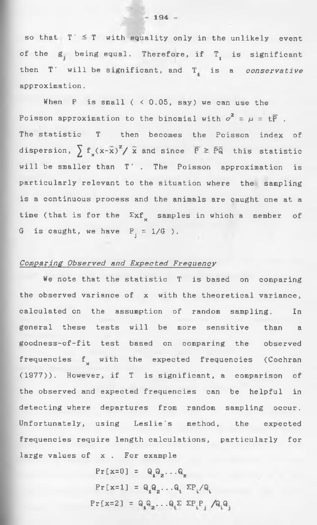
194

so that T' ^ T with equality only in the unlikely event

of the g. being equal. Therefore, if T± is significant

then T' will be significant, and T is a c o n s e r v a t i v e approximation.

When P is small ( < 0.05, say) we can use the

Poisson approximation to the binomial with o 2 - p = tP .

The statistic T then becomes the Poisson index of

dispersion, ^ fx(x-x)2/ x and since P > PQ this statistic

will be smaller than T' . The Poisson approximation is

particularly relevant to the situation where the sampling

is a continuous process and the animals are caught one at a

time (that is for the £xf samples in which a member ofX

G is caught, we have P = 1/G ).

C o m p a r i n g O b s e r v e d a n d E x p e c t e d F r e q u e n c y

We note that the statistic T is based on comparing

the observed variance of x with the theoretical variance,

calculated on the assumption of random sampling. In

general these tests will be more sensitive than a

goodness-of-fit test based on comparing the observed

frequencies fX

with the expected frequencies (Cochran

(1977)). However, if T is significant, a comparison of

the observed and expected frequencies can be helpful in

detecting where departures from random sampling occur.

Unfortunately, using Leslie's method, the expected

frequencies require length calculations, particularly for

large values of x . For example

Pr[x=0] = Q Q ...Q1 2 Z

Pr [x=i] = q 1q 2 ...q 1 a y e ,Pr[x=2] = Q Q ...QZ ZP.P. /Q Q.

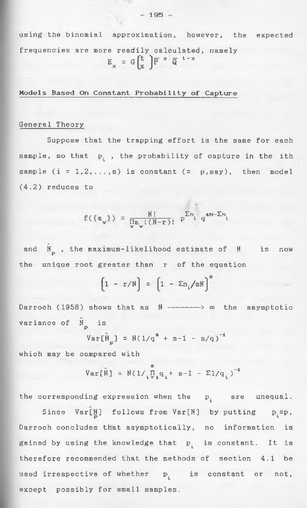
195

using the b

frequencies

inomial

are more E

approximation, however, the

readily calculated, namely

expected

Models Based On Constant Probability of Capture

General Theory

Suppose that the trapping effort is the same for each

sample, so that p^ , the probability of capture in the ith

sample (i = l,2 ,...,s) is constant (= p,say), then model

(4.2) reduces to

N!na !(N-r ) !V V

Zn. sN-Zn p v q v

and N , the maximum-likelihood estimate of N is nowpthe unique root greater than r of the equation

fl - r / N j = £l - Zr\ ./■»)

Darroch (1958) shows that as N ------- > oo the asymptoticA

variance of N ispVar[N ] = N(l/qs + s-1 - s/q) ' 1P

which may be compared withs

Var[N] = N(l/.n q.+ s-1 - ri/q . ) " 1V = 1 t V

the corresponding expression when the pt are unequal.

Since Var[N] follows from Var[N] by putting P =P,p v.Darroch concludes that asymptotically, no information is

gained by using the knowledge that p is constant. It is

therefore recommended that the methods of section 4.1 be

used irrespective of whether pt is constant or not,

except possibly for small samples.

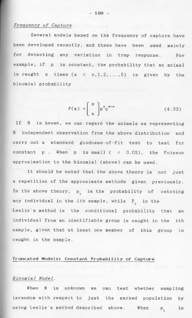
196

F r e q u e n c y o f C a p t u r e

Several models based on the frequency of capture have

been developed recently, and these have been used mainly

for detecting any variation in trap response. For

example, if p is constant, the probability that an animalI

is caught x times (x = o,l,2,...,5) is given by the

binomial probability

f(x) x s-xp q (4.33)U J

If N is known, we can regard the animals as representing

N independent observation from the above distribution and

carry out a standard goodness-of-fit test to test for

constant p . When p is small ( < 0.05), the Poisson

approximation to the binomial (above) can be used.

It should be noted that the above theory is not just

a repetition of the approximate methods given previously.

In the above theory, pt is the probability of catching

any individual in the ith sample, while P in the

Leslie's method is the conditional probability that an

individual from an identifiable group is caught in the ith

sample, given that at least one member of this group is

caught in the sample.

Truncated Models: Constant Probability of Capture

B i n o m i a l M o d e l .

When N is unknown we can test whether sampling

israndom with respect to just the marked population by

using Leslie's method described above. When p ist

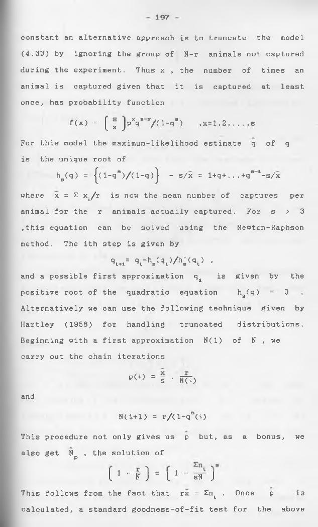
197

constant an alternative approach is to truncate the model

(4.33) by ignoring the group of N-r animals not captured

during the experiment. Thus x , the number of times an

animal is captured given that it is captured at least

once, has probability function

f(x) = [ x ] p X q S * A l - q S ) , x = l , 2 , . . . , s

For this model the maximum-likelihood estimate q of q

is the unique root of

hs(q) - |(i-qs)/(i-q)| - s/x = i+q+...+qs 4-s/x

where x = £ x^/r is now the mean number of captures per

animal for the r animals actually captured. For s > 3

,this equation can be solved using the Newton-Raphson

method. The ith step is given by

qi+l= V hs(V / hs(V 'and a possible first approximation q ± is given by the

positive root of the quadratic equation h3(q) = 0

Alternatively we can use the following technique given by

Hartley (1958) for handling truncated distributions.

Beginning with a first approximation N(l) of N , we

carry out the chain iterations

p(l) = S’ • iuT)

and

N(i+1) = r/(l-qs(i)

This procedure not only gives us p but, as a bonus, we

also get N , the solution ofp

is

! i - — 11 = ■ 1 - — - 1l N J1 L sN JThis follows from the fact that rx = £n^ . Once p

calculated, a standard g o o d n e s s - o f - f i t test for the above

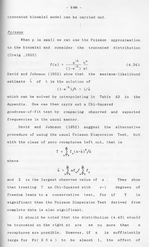
198

truncated binomial model can be carried out.

P o i s s o n

When p is small we can use the Poisson approximation

to the binomial and consider the truncated distribution

(Craig ,1953)

f(x) = ---^-5— — (4.34)(1 -e ) x!

David and Johnson (1952) show that the maximum-likelihoodA

estimate X of X is the solution of

(l-e'X )/X = 1/i

which can be solved by interpolating in Table A3 in the

Appendix. One can then carry out a Chi-Squared

goodness-of-fit test by comparing observed and expected

frequencies in the usual manner.

David and Johnson (1952) suggest the alternative

procedure of using the usual Poisson Dispersion Test, but

with the class of zero recaptures left out, that isx

t = J fx(x-;>7 iX = i

where

and X is the largest observed value of x . They show

that treating T as Chi-Squared with r- 1 degrees of

freedom leads to a conservative test, for if T is

significant then the Poisson Dispersion Test derived from

complete data is also significant.

It should be noted that the distribution (4.43) should

be truncated on the right at x=s as no more than s

recaptures are possible. However, if s is sufficiently

large for Pr( X ^ s ) to be almost 1, the effect of

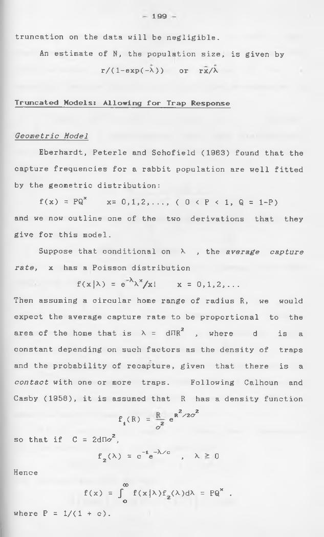
199

truncation on the data will be negligible.

An estimate of N, the population size, is given by

r/(l-exp(-X)) or rx/X

Truncated Models: Allowing for Trap Response

G e o m e t r i c Model

Eberhardt, Peterle and Schofield (1963) found that the

capture frequencies for a rabbit population are well fitted

by the geometric distribution:

f(x ) = PQX x= 0,1,2,..., ( 0 < P < 1, Q = 1-P)

and we now outline one of the two derivations that they

give for this model.

Suppose that conditional on X , the a v e r a g e capture

r a t e , x has a Poisson distribution

f(x|X) = e ^Xx/x! x = 0,1,2,...

Then assuming a circular home range of radius R, we would

expect the average capture rate to be proportional to the. 2area of the home that is X = dflR , where d is a

constant depending on such factors as the density of traps

and the probability of recapture, given that there is a

c o ntact with one or more traps. Following Calhoun and

Casby (1958), it is assumed that R has a density function

f,(R) = eR W o

so that if C = 2dncyz,

fz( M = c ' V Xxe , X > 0

Henceco

f(x) = f f(x|X)f (X)dX = PQX . o

where P = 1/(1 + c).

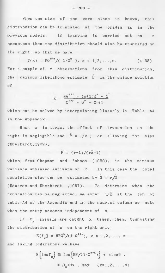
200

When the size of the zero class is known, thisdistribution can be truncated at the origin as in theprevious models. If trapping is carried out on s

occasions then the distribution should also be truncated on

the right, so that we have

f(x) = PQX */( 1-QS ), x = 1,2,...,s . (4.35)

For a sample of r observations from this distribution,

the maximum-likelihood estimate P is the unique solution

of

- = sQs+1 - (s+l)Qs + 1

Qs+1 - Qs - Q +1

which can be solved by interpolating linearly in Table A4

in the Appendix.

When s is large, the effect of truncation on the

right is negligible and P = 1/x ; or allowing for bias

(Eberhardt,1969),

P = (r-l)/(rx-1)

which, from Chapman and Robson (1960), is the minimum

variance unbiased estimate of P . In this case the total

population size can be estimated by N = r/Q

(Edwards and Eberhardt ,1967). To determine when the

truncation can be neglected, we enter 1/x at the top of

table A4 of the Appendix and in the nearest column we note

when the entry becomes independent of s .

If f animals are caught x times, then, truncating

the distribution of x on the right only,

E[fx] = NPQX/(1-QS+1), x = 1,2,..., s

and taking logarithms we have

E flogfxj 3 logfNP/a-Q3"1)] + xlogQ .

= ft +/?x > say (x=l, 2 , . . . , s )

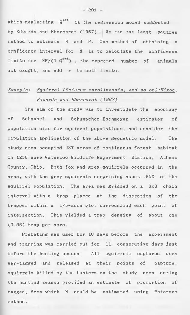
201

S + iwhich neglecting Q is the regression model suggested

by Edwards and Eberhardt (1967). We can use least squares

method to estimate N and P. One method of obtaining a

confidence interval for N is to calculate the confidence

limits for NP/(1-Q ) , the expected number of animals

not caught, and add r to both limits.

E x a m p l e : Squirrel (Sciurus c a r o l i n e n s i s, a nd so o n ) : N i x o n ,

E d w a r d s a n d E b e r h a r d t (1967)

The aim of the study was to investigate the accuracy

of Schnabel and Schumacher-Eschmeyer estimates of

population size for squirrel populations, and consider the

population application of the above geometric model. The

study area occupied 237 acres of continuous forest habitat

in 1250 acre Waterloo Wildlife Experiment Station, Athens

County, Ohio. Both fox and grey squirrels occurred in the

area, with the grey squirrels comprising about 95% of the

squirrel population. The area was gridded on a 3x3 chain

interval with a trap placed at the discretion of the

trapper within a 1/5-acre plot surrounding each point of

intersection. This yielded a trap density of about one

(0.96) trap per acre.

Prebating was used for 10 days before the experiment

and trapping was carried out for 1 1 consecutive days just

before the hunting season. All squirrels captured were

ear-tagged and released at their points of capture,

squirrels killed by the hunters on the study area during

the hunting season provided an estimate of proportion of

tagged, from which N could be estimated using Petersen

method.

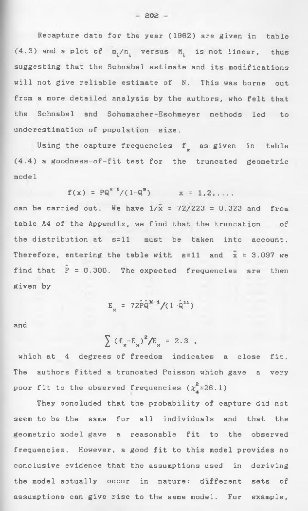
202

Recapture data for the year (1962) are given in table

(4.3) and a plot of m^n^ versus ht is not linear, thus

suggesting that the Schnabel estimate and its modifications

will not give reliable estimate of N. This was borne out

from a more detailed analysis by the authors, who felt that

the Schnabel and Schumacher-Eschmeyer methods led to

underestimation of population size.

Using the capture frequencies f as given in tableX

(4.4) a goodness-of-fit test for the truncated geometric

model

f(x) = PQX'V(1-Q") X = 1,2,___can be carried out. We have 1/x = 72/223 = 0.323 and from

table A4 of the Appendix, we find that the truncation of

the distribution at s=ll must be taken into account.

Therefore, entering the table with s = ll and x = 3.097 we

find that P = 0.300. The expected frequencies are then

given byA * V—I * 4 4Ex = 72PQ /(1 -Q )

and

1 < w X = 2 - 3 •which at 4 degrees of freedom indicates a close fit.

The authors fitted a truncated Poisson which gave a very2poor fit to the observed frequencies (x =26.1)

They concluded that the probability of capture did not

seem to be the same for all individuals and that the

geometric model gave a reasonable fit to the observed

frequencies. However, a good fit to this model provides no

conclusive evidence that the assumptions used in deriving

the model actually occur in nature: different sets of

assumptions can give rise to the same model. For example,

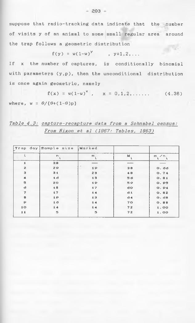
203

suppose that radio-tracking data indicate that the number

of visits y of an animal to some small regular area around

the trap follows a geometric distribution

f(y) = w(l-w)y , y=l,2 ,...

If x the number of captures, is conditionally binomial

with parameters (y,p), then the unconditional distribution

is once again geometric, namely

f(x) = w(l-w)x , x = 0,1,2,..... (4.36)

where, w = 0 / { 6 + ( l-0 )p}

Table 4.3: c a p t u r e - r e c a p t u r e data fro m a Schnabel census: F r o m N i x o n et al (1967: Tables, 1963)

T rap day S a m p l e s i z e M a r k edi n m M m / r\L V v t1 38 — — —2 2 P 1 P 3 8 O. <5<53 3 1 23 4 8 O. 744 1 <5 1 3 5 <5 0.8 15 20 1 P 5 P O. P5<5 1 8 1 7 <50 O. 947 17 1 4 <5 1 O. 828 1 P 1 3 <54 O. <58P 1 <5 1 4 70 O. 88

IO 1 4 1 4 72 1 . OO11 5 5 72 1 . OO

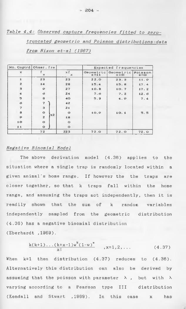
204

Table 4.4: O b s e r v e d c a p ture f r e q u e n c i e s f i t t e d to zero-

truncated g e o m e t r i c a nd P o i s s o n d i s t r i b u t i o n s : d a t a from N i x o n et-al (1967)

N o . C a p t r d O b s e r . f r © E x p e c t e d f r e q u e n c i e sX f x f O e o m e t r i c O e o m e t r i e P o i s s o n

X X s = 1 1 S = 0 0 s = CO

1 2 3 2 3 2 2 . 0 2 3 . 3 1 1 . P2 1 4 2 8 1 5 . 4 1 5 . 8 1 7 . 43 P 2 7 1 0 . 8 I O . 7 1 7 . 2

4 <5 2 4 7. <5 7 . 2 1 2 . <5

5 8 4 0 5 . 3 4 . P 7 . 4<5 7 ] 4 2

7 3 2 1

B O O I O . P I O . 1 5 . 5►12

P 2 1 8

io O O

1 1 _______ p j O

7 2 2 2 3 7 2 . 0 7 2 . O 7 2 . O

N e g a t i v e B i n o m i a l Model

The above derivation model (4.36) applies to the

situation where a single trap is randomly located within a

given animal's home range. If however the the traps are

closer together, so that k traps fall within the home

range, and assuming the traps act independently, then it is

readily shown that the sum of k random variables

independently sampled from the geometric distribution

(4.36) has a negative binomial distribution

(Eberhardt ,1969).

k(k+l). . .(k|x-l)wk(l-w)x >x=1>2> _ (4 .3 7 )

When k=l then distribution (4.37) reduces to (4.36).

Alternatively this distribution can also be derived by

assuming that the poisson with parameter X , but with X

varying according to a Pearson type III distribution

(Kendall and Stwart ,1969). In this case x has

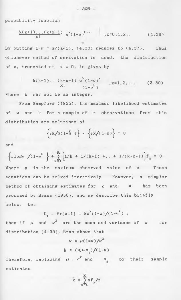
205

probability function

k( k+1) . . . ( k+x-1) X/i. xk+x— -----— j— ----- a (1+a)xl ,x=0 ,1 ,2 .. (4.38)

By putting 1-w = a/(a+l), (4.38) reduces to (4.37). Thus

whichever method of derivation is used, the distribution

of x, truncated at x = 0 , is given by

k(k+1)...(k+x-1) wk(1—w )* 1 9I V » x >( 1 -w )x! (3.39)

Where k may not be an integer.

From Sampford (1955), the maximum likelihood estimates

of w and k for a sample of r observations from this

distribution are solutions of

jrk/w(l-w )j - jrx/(l-w)j = 0

and

jrlogw /( 1 -wk | + | £l/k + l/( k+1 ) +...+ l/( k+x- 1 )j = 0

Where x is the maximum observed value of x. These

equations can be solved iteratively. However, a simpler

method of obtaining estimates for k and w has been

proposed by Brass (1958), and we describe this briefly

below. Let

T\± = Pr[x=l] = kwk(l-w)/(l-wk) ;2then if ^ and o are the mean and variance of x for

distribution (4.39), Bras shows that2w =

k = (w m -^1)/(1-w)Therefore, replacing fj , o'2 and re by their sample

estimates

xf /rX = 1

X

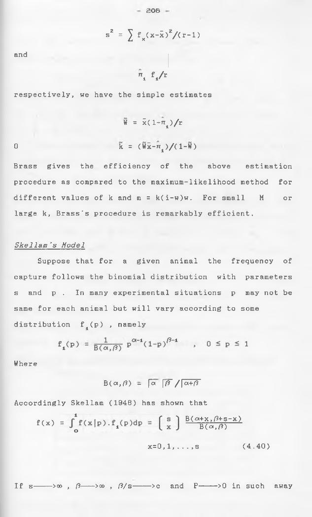
206

s2 = J fx(x-i)z/(r-l)

and

n i

respectively, we have the simple estimates

0

W = i d - r r ^ / r

k = (Wi-n±)/(l-W)

Brass gives the efficiency of the above estimation

procedure as compared to the maximum-likelihood method for

large k, Brass's procedure is remarkably efficient.

S k e l l a m 's Model

Suppose that for a given animal the frequency of

capture follows the binomial distribution with parameters

s and p . In many experimental situations p may not be

same for each animal but will vary according to some

distribution f±(p) > namely

different values of k and m = k(i-w)w. For small M or

Where

B(ot,^) - [a [fT /| a+{3

Accordingly Skellam (1948) has shown that

f(x) B(oi+x, /3+s-x) B(«,0 )

x=0 ,1 , . . . , s (4.40)

If s >00 , (3--->00 , (3/s >c and P >0 in such away

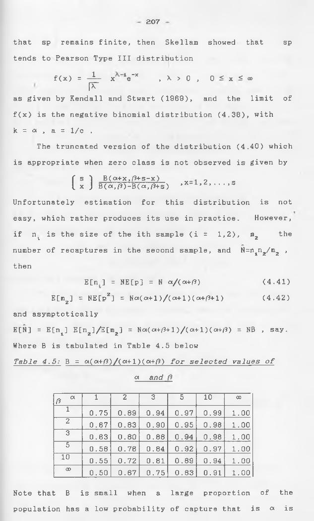
207

that sp remains finite, then Skellam showed that sp

tends to Pearson Type III distribution

rt / \ I 1 "Xf (x) = --- x e , X > 0 , 0 < x < ooF

as given by Kendall and Stwart (1969), and the limit of

f(x) is the negative binomial distribution (4.38), with

k = a , a = 1 /c .

The truncated version of the distribution (4.40) which

is appropriate when zero class is not observed is given by

f s 1 B(ot+x,ft+s-x) 1 9l x J B(a,0 )-B(a,0+s) 'X"1'Z***',S

Unfortunately estimation for this distribution is not

easy, which rather produces its use in practice. However,

if n^ is the size of the ith sample (i = 1 ,2 ), m2 the

number of recaptures in the second sample, and N=nin2/m2 ,

then

E[n.] = NE[p] = N a/(a+0) (4.41)

E[mz] = NE[p2] = Na( cx+1 ) /(a+ 1 ) (a+f3+1 ) (4.42)

and asymptotically

E[N] = E[n±] E[n2]/E[m2] = Na(af/3+l)/(a+l)(a+/3) = NB , say.

Where B is tabulated in Table 4.5 below

Table 4.5: B = ot(ot+ft)/(ot+l)(ot+ft) for s e l e c t e d values of

ot and

(5 ° 1 2 3 5 1 0 00

1 0.75 0.89 0.94 0.97 0.99 1 . 0 02 0.67 0.83 0.90 0.95 0.98 1 . 0 03 0.63 0.80 0 . 8 8 0.94 0.98 1 . 0 05 0.58 0.76 0.84 0.92 0.97 1 . 0 0

10 0.55 0.72 0.81 0.89 0.94 1 . 0 000 0.50 0.67 0.75 0.83 0.91 1 . 0 0

Note that B is small when a large proportion of the

population has a low probability of capture that is a is

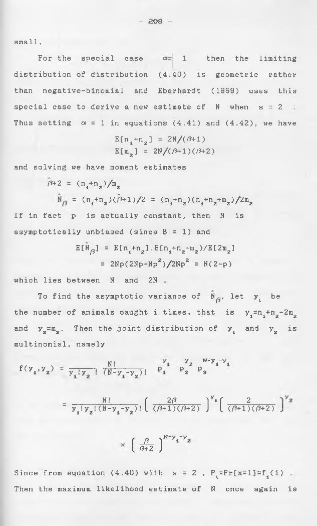
- 208 -

then the limiting

small.

For the special case a- 1

distribution of distribution (4.40) is geometric rather

than negative-binomial and Eberhardt (1969) uses this

special case to derive a new estimate of N when s = 2

Thus setting a = 1 in equations (4.41) and (4.42), we have

E [n ±+n 2 ] = 2N/(/?+l)E[mz] = 2N/(0+l)O?+2)

and solving we have moment estimates

/ ?+2 = (ni+n2 )/m2

= (n±+n2 )(^+l) / 2 = (ni+n2 )(ni+n2+m2 )/2m2

If in fact p is actually constant, then N is

asymptotically unbiased (since B = 1) and

E[N^] = E[n±+n2] .E[n±+n2-m2 )/E[2m2]

= 2Np(2Np-Npz)/2Npz = N(2 -p)

which lies between N and 2N .

To find the asymptotic variance of N^, let y be

the number of animals caught i times, that is y =n +n -2m„1 1 2 2

y =m . Then the joint distribution of y and y is 2 2 1 2

and

multinomial, namely

N if(yi'y2 ) " y !y ! (N-y -y„)!

y N-y -y *2. * 1 P P2 3

N! f 2ft lyif 2" yi!y2 !(N-yi-y2)! L <(?+l)<(3+2) J L </3+l)</?+2) J

N-y -y.

(A) ‘Since from equation (4.40) with s = 2 , Pi=Pr[x=l] =f±( i)

Then the maximum likelihood estimate of N once again is

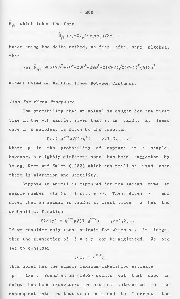
209

which takes the form

(y1+2y2 )(y1+y2 )/2yz .

Hence using the delta method, we find, after some algebra,

that

VarCN^] 2= N/?(/35+7^4+20tf3+29^2+21f?+6)/2(fJ+l)2(^+2)2

Models Based on Waiting Times Between Captures.

Time for F i r s t R e c a p t u r e

The probability that an animal is caught for the first

time in the yth sample, given that it is caught at least

once in s samples, is given by the function

f(y) <3ylp/(l-qs) , y=l, 2 , . . . , s

Where p is the probability of capture in a sample.

However, a slightly different model has been suggested by

Young, Nees and Emlen (1952) which can still be used when

there is migration and mortality.

Suppose an animal is captured for the second time in

sample number y+z (z = 1 ,2 , . ..s-y). Then, given y and

given that an animal is caught at least twice, z has the

probability function

f ( z | y ) = qzlp/(l-qs y ) , z = l, 2 , . . .

If we consider only those animals for which s-y is large,

then the truncation of Z = s-y can be neglected. We are

led to consider

f(z) = q p

This model has the simple maximum-likelihood estimate

P = 1/z . Young et al (1952) points out that once an

animal has been recaptured, we are not interested in its

subsequent fate, so that we do not need to "correct" the

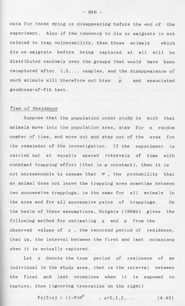
210

data for those dying or disappearing before the end of the

experiment. Also if the tendency to die or emigrate is not

related to trap vulnerability, then those animals which

die or emigrate before being captured at all will be

distributed randomly over the groups that would have been

recaptured after 1 ,2 ,... samples, and the disappearance of

such animals will therefore not bias p and associated

goodness-of-fit test.

Time o f Res i d e n c e

Suppose that the population under study is such thatanimals move into the population area, stay for a randomnumber of time, and move out and stay out of the area forthe remainder of the investigation. If the experiment iscarried out at equally spaced intervals of time with

constant trapping effort (that is p constant), then it is

not unreasonable to assume that O , the probability that

an animal does not leave the trapping area sometime between

two successive trappings, is the same for all animals in

the area and for all successive pairs of trappings. On

the basis of these assumptions, Holgate (1964b) gives the

following method for estimating q and p from the

observed values of y , the recorded period of residence,

that is, the interval between the first and last occasions

when it is actually captured.

Let z denote the true period of residence of an

individual in the study area, that is the interval between

the first and last occasions when it is exposed to

capture; then (ignoring truncation on the right)

Pr[Z=z] = (l-e)ez z = 0 ,1 ,2 ,... (4.43)

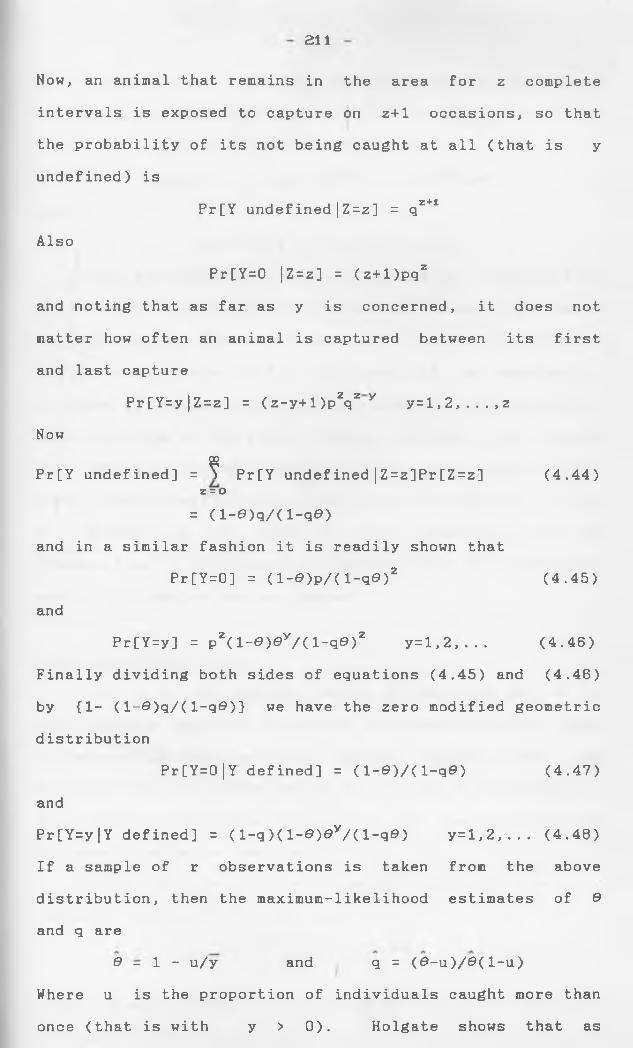
211

Now, an animal that remains in the area for z complete

intervals is exposed to capture on z+ 1 occasions, so that

the probability of its not being caught at all (that is y

undefined) is

Pr[Y undefined |Z = z] = qz+1

Also

Pr[Y=0 |Z=z] = (z+l)pqz

and noting that as far as y is concerned, it does not

matter how often an animal is captured between its first

and last capture

Pr[Y=y|Z=z] = (z-y+l)p2qzy y=l,2,...,z

Now

Pr[Y undefined] = ? Pr[Y undefined|Z=z]Pr[Z=z] (4.44)z = O

= (l-6»q/(l-q0 )and in a similar fashion it is readily shown that

Pr[Y=0] = (l-0)p/(l-qe)Z (4.45)

and

Pr[Y=y] = p2(l-e)ey/(l-qe) 2 y=l,2, . . . (4.46)

Finally dividing both sides of equations (4.45) and (4.46)

by {1 - (l-0 )q/(l-q^)} we have the zero modified geometric

distribution

Pr[Y=0|Y defined] = (l-3)/(l-q0) (4.47)

and

Pr[Y=y|Y defined] = (1-q)(l-e)0y/(1 -qS) y=l,2,... (4.48)

If a sample of r observations is taken from the above

distribution, then the maximum-likelihood estimates of O and q are

O - 1 - u/y and q = (O - u ) / & ( 1 -u)

Where u is the proportion of individuals caught more than

once (that is with y > 0). Holgate shows that as

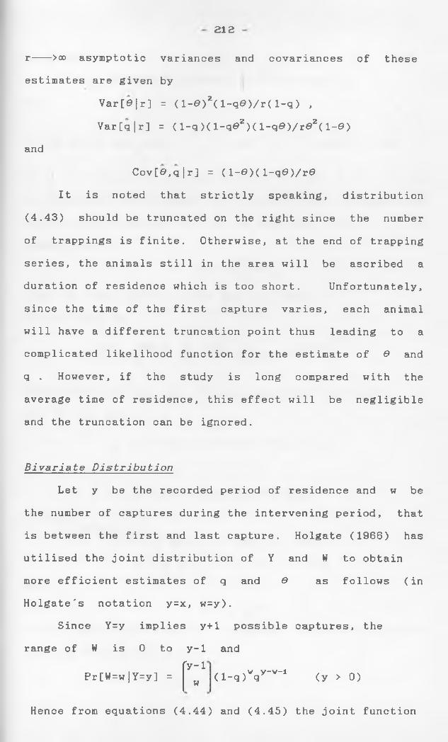
212

r--->oo asymptotic variances and covariances of these

estimates are given by

Var[e|r] = ( l-0 )2( l-q0 )/r< 1 -q ) ,

Var[q|r] = (1-q)(l-q02 )(l-q0)/r02(1-0)

and

Cov[0 ,q|r] = (l-0 )(l-q0 )/r0

It is noted that strictly speaking, distribution

(4.43) should be truncated on the right since the number

of trappings is finite. Otherwise, at the end of trapping

series, the animals still in the area will be ascribed a

duration of residence which is too short. Unfortunately,

since the time of the first capture varies, each animal

will have a different truncation point thus leading to a

complicated likelihood function for the estimate of O and

q . However, if the study is long compared with the

average time of residence, this effect will be negligible

and the truncation can be ignored.

B i v a r i a t e D i s t r i b u t i o n

Let y be the recorded period of residence and w be

the number of captures during the intervening period, that

is between the first and last capture. Holgate (1966) has

utilised the joint distribution of Y and W to obtain

more efficient estimates of q and O as follows (in

Holgate's notation y=x, w=y).

Since Y=y implies y+1 possible captures, the

range of W is 0 to y - 1 andfy-i

Pr[W=w|Y=y] = w/ 1 \w y~v_1(1-q) q (y > 0)

Hence from equations (4.44) and (4.45) the joint function

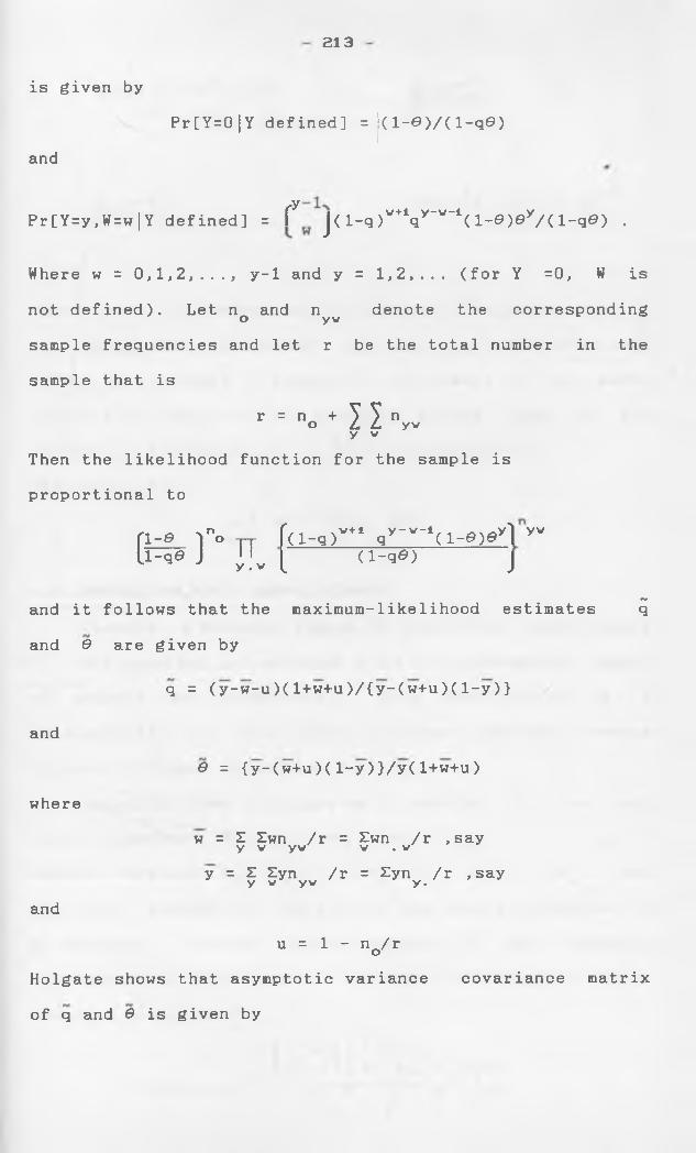
213

is given by

and

Pr[Y=0|Y defined] = <l-0 )/(l-q0 )

Pr[Y=y,W=w | Y defined] = f j{ 1-q )W+V ' W'‘( l-©)ey/<l-qe> .

Where w = 0,1,2,..., y-1 and y = 1,2,... (for Y =0, W is

not defined). Let n and n denote the correspondingO ywsample frequencies and let r be the total number in the

sample that is

r = no + 1 1 n yv y vThen the likelihood function for the sample is

proportional to

f l - 0 f o -pp f ( 1 - q ) v+1 q y " v ~1( l - ^ ) ^ ylU - q e J ; ; v { ( i - q * > J

yv

and it follows that the maximum-likelihood estimates

and O are given by

q = (y-w-u)(1 +w+u)/(y-(w+u)(1 -y ) }

and

where

e = (y-(w+u)(l-y)}/y(1 +w+u)

w = Z Zwn /r = £wn /r ,sayy v yv v . v

y = Z Zyn /r = £yn /r ,sayy v y v y.

and

u = 1 - nQ/r

Holgate shows that asymptotic variance

of q and 0 is given by

covariance matrix

e cr

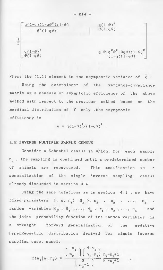
214

q(l-q)(l-qe2 )(l-e)© 2 ( l - q © )

1r

q(i-e)3S(l-q©)

g(i-Q) 3S d - q S )

q+e+q2e2-3qe)(i-e)2(l-q)(l-q0 )

Where the (1,1) element is the asymptotic variance of q .

Using the determinant of the variance-covariance

matrix as a measure of asymptotic efficiency of the above

method with respect to the previous method based on the

marginal distribution of Y only ,the asymptotic

efficiency is

e = q(l-e)2/(l-q6>)2 .

4.2 INVERSE MULTIPLE SAMPLE CENSUSConsider a Schnabel census in which, for each sample

n , the sampling is continued until a predetermined number

of animals are recaptured. This modification is a

generalization of the simple inverse sampling census

already discussed in section 3.4.

Using the same notations as in section 4.1 , we have

fixed parameters N, s, n ( =M, ), in , m , ..., m ,

random variables M . r , n ,...,n andO 4 S 1 2 S

the joint probability function of the random variables is

a straight forward generalisation of the negative

hypergeometric distribution derived for simple inverse

sampling case, namelyN-n

f(n2 |nt,n2)( ">2 -l) [ n2-mj

( 7 7 * )'N -n +1 2

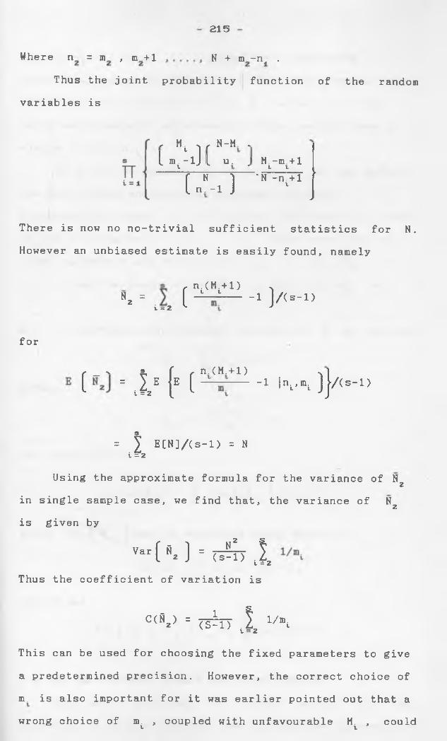
215

Where n = m , m + 1 N + m -n, .

Thus the joint probability function of the random variables is

, M . r N-M ,1 ^ 1

[ m -lj L u. j M - m +1v t * i ir N i ■ N -n +1 ’1 n.-l J

tJ

There is now no no-trivial sufficient statistics for N.

However an unbiased estimate is easily found, namely

"z = i = 2r ni<Mi+1> 'i ( -1 )/<s-l)

for

r _ -v s f n.(M. + l)( = j 2 E { E ( - 1 I V i ] | / < s _ 1 >

s= J E[N]/(s-l) = N

i = 2

Using the approximate formula for the variance of N2

in single sample case, we find that, the variance of N2

is given by

V a r K ) = c i S y X

Thus the coefficient of variation is

C(S2 } = (s^iy 1 1/miv i = 2

This can be used for choosing the fixed parameters to give

a predetermined precision. However, the correct choice of

nr is also important for it was earlier pointed out that a

wrong choice of m. , coupled with unfavourable M. ,i t could

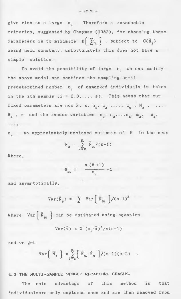
216

give rise to a large rr . Therefore a reasonable

criterion, suggested by Chapman (1952), for choosing these

parameters is to minimize E ( K ) , subject to C(N2)

being held constant; unfortunately this does not have a

simple solution.

To avoid the possibility of large n we can modify

the above model and continue the sampling until

predetermined number u of unmarked individuals is taken

in the ith sample (i = 2,3,..., s). This means that our

fixed parameters are now N, s, n , u2 ug , M3 , ...,

M , r and the random variables n , n , . . .n , m . m .S 2 3 S Z . 3

m . An approximately unbiased estimate of N is the meanS

S3 = 1 » * / < ■ - ! >1 = 2Where,

3in. (M. + l)V t

m. - 1

and asymptotically,

Var(N3) = J Var( j A 5’1)'

Where Var ( &3t) can be estimated using equation

Var(x) = £ (x^-x)Z/n(n-l)

and we get

’ “ I “a ) = t l 2 ( "3TS3 J/CS-DCS-2) •

4.3 THE MULTI-SAMPLE SINGLE RECAPTURE CENSUS.The main advantage of this method is that

individualsare only captured once and are then removed from

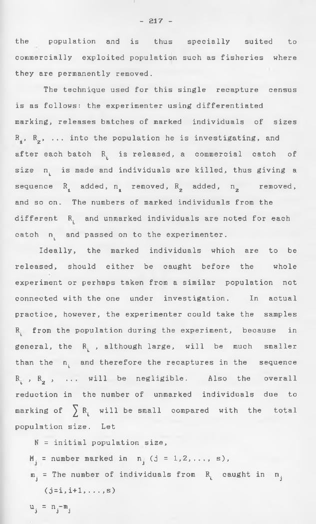
the population and is thus specially suited to

commercially exploited population such as fisheries where

they are permanently removed.

The technique used for this single recapture census

is as follows: the experimenter using differentiated

marking, releases batches of marked individuals of sizes

R , R2, ... into the population he is investigating, and

after each batch R is released, a commercial catch of

size n is made and individuals are killed, thus giving a

sequence R± added, n± removed, R2 added, n2 removed,

and so on. The numbers of marked individuals from the

different R. and unmarked individuals are noted for each

catch n and passed on to the experimenter.

Ideally, the marked individuals which are to be

released, should either be caught before the whole

experiment or perhaps taken from a similar population not

connected with the one under investigation. In actual

practice, however, the experimenter could take the samples

R from the population during the experiment, because in

general, the Ri , although large, will be much smaller

than the nL and therefore the recaptures in the sequence

R , Rz , ... will be negligible. Also the overall

reduction in the number of unmarked individuals due to

marking of ^ Rt will be small compared with the total

population size. Let

N = initial population size,

hT = number marked in nj (j = 1 ,2 ,..., s),

m = The number of individuals from R. caught in n. j * J

(j=i,i+1 ,...,s)

u. = n.-m. j j j

'

- 217 -

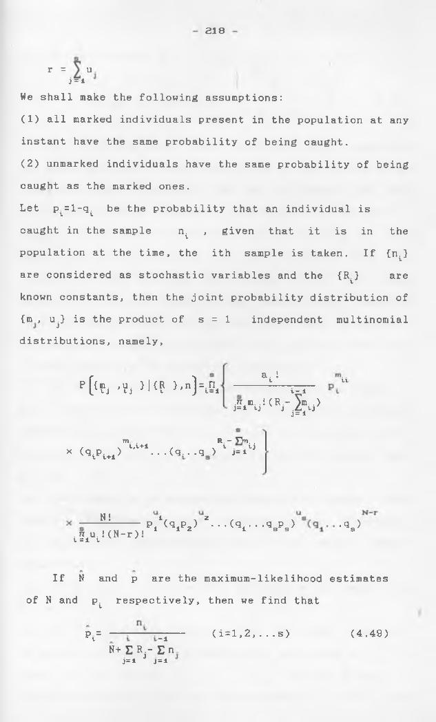
218

r = uj = i

We shall make the following assumptions:

(1 ) all marked individuals present in the population at any

instant have the same probability of being caught.

(2 ) unmarked individuals have the same probability of being

caught as the marked ones.

Let p^=l-qi be the probability that an individual is

caught in the sample n i , given that it is in the

population at the time, the ith sample is taken. If {nt}

are considered as stochastic variables and the {R.} aretknown constants, then the joint probability distribution of

{m., u^ is the product of s = 1 independent multinomial

distributions, namely,

pf{m. , u . } | (R } , nl =.nL t J IJ 1 V J V=1

a. it tti-1

.n m..! ( R - ym .)j = i i j ' j X i jj= i

m . R - TVi. ., . v,v+l , . v tjx (q;p; ) . .. (q;. .q ) j=*t l+l

Ni. n U. ! (N-r)ii =i t

Pi‘<qiP2) Z---(<31---'3SPS) -<3.)

If N and p are the maximum-likelihood estimates

of N and p l respectively, then we find that

PV= - 1 (i=l,2,...s ) (4.49)N+ E Rj- E n

j=* j=i

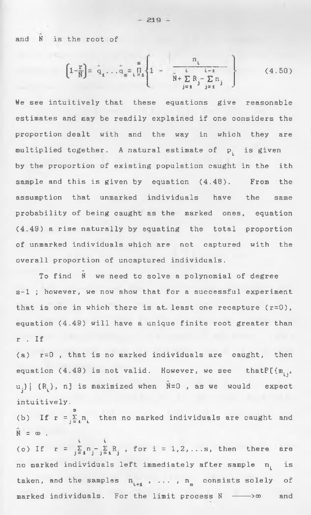
219

and N is the root of

q . . . q = . FI ^1 1 =1

n.vi i-i

H + E R - E n . j , jj=i j=i

► (4.50)

We see intuitively that these equations give reasonable

estimates and may be readily explained if one considers the

proportion dealt with and the way in which they are

multiplied together. A natural estimate of Pt is given

by the proportion of existing population caught in the ith

sample and this is given by equation (4.48). From the

assumption that unmarked individuals have the same

probability of being caught as the marked ones, equation

(4.49) a rise naturally by equating the total proportion

of unmarked individuals which are not captured with the

overall proportion of uncaptured individuals.a

To find N we need to solve a polynomial of degree

s- 1 ; however, we now show that for a successful experiment

that is one in which there is at- least one recapture (r=0 ),

equation (4.49) will have a unique finite root greater than

r . If

(a) r=0 , that is no marked individuals are caught, then

equation (4.49) is not valid. However, we see thatP[{m^,

u .} | (R.}, n] is maximized when N=0 , as we would expectj lintuitively.

s(b) If r = J|:int then no marked individuals are caught and N = oo .

i i(c) If r = .Z n.-.Z R. , for i = l,2,...s, then there arej = i j j = i jno marked individuals left immediately after sample nL is

taken, and the samples , ... , ns consists solely of

marked individuals. For the limit process N >oo and

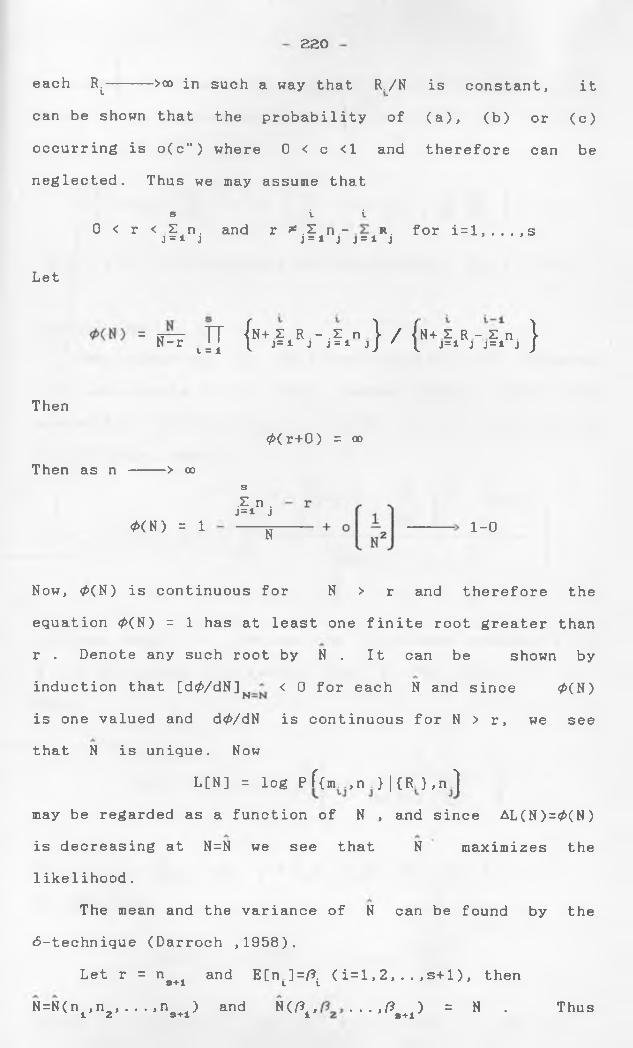
220

each R.----- >oo in suchV a way that R.yN is constant, itcan be shown that the probability of (a), (b) or (c)occurring is o(cM) where 0 < c < 1 and therefore can beneglected. Thus we may assume that

s0 < r < Z n. andj = i j

i ir ^ .51 n - r .j = i j j = i j for i=l,...,s

Let

= N-r TT {1 = 1 'N+Z R.-.Z n ) /j=i j j = i jJ ' |n+ Z R - Z n } t J=1 j J=1 j J

Then

Then as n ----> oo

0(N) = 1

<P( r+0 ) = oo

3X n . j=i j

N 1 - 0

Now, <£(N) is continuous for N > r and therefore the

equation <£(N) = 1 has at least one finite root greater than

r . Denote any such root by N . It can be shown by

induction that [d0/dN]N < 0 for each N and since <£(N)

is one valued and d<£/dN is continuous for N > r, we see

that N is unique. Now

L[N] = log pf{m ,n } |{R },n]

may be regarded as a function of N , and since AL(N)=<£(N)

is decreasing at N=N we see that N maximizes the

likelihood.

The mean and the variance of N can be found by the

6-technique (Darroch ,1958).

Let r = ng+i and E[n^]=^ ( i=l, 2, . . , s+1) , then

N=N(ni,nz, . . . ,ns+i) and N(^, . . . , fts+±) = N . Thus

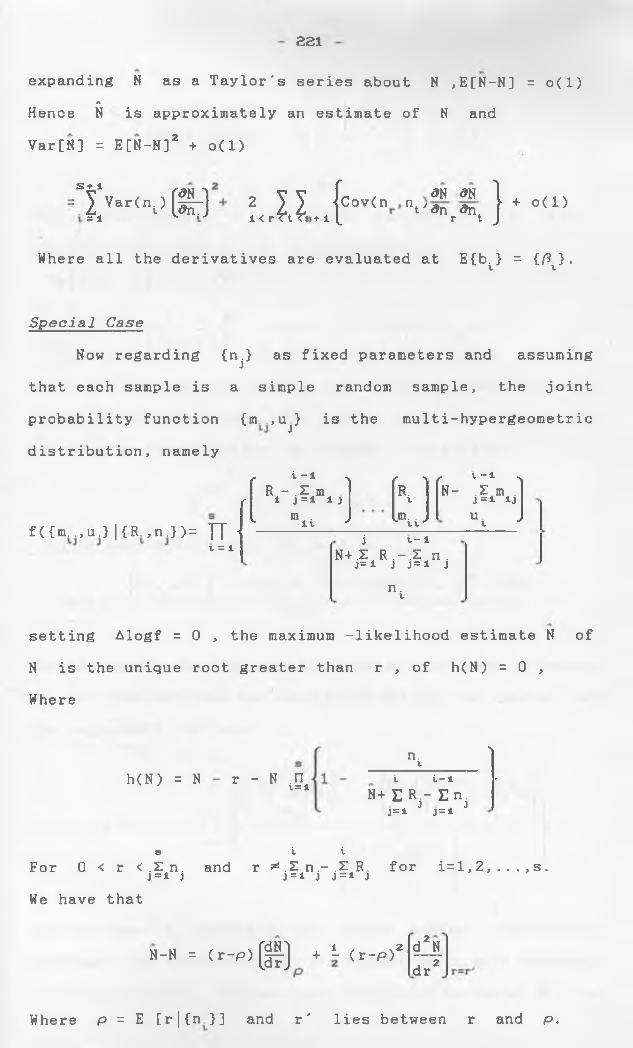
221

expanding N as a Taylor's series about N ,E[N-N] = o(l)a

Hence N is approximately an estimate of N and

Var[N] = E[N-N] 2 + o(l)

S + 1

- 1VarCn^) (§ e i l l J

Cov(n aN mnt ' # n anr . } + 0 ( 1 )

Where all the derivatives are evaluated at E{b.} = {ft.}.t t

Special Case

Now regarding {n } as fixed parameters and assuming

that each sample is a simple random sample, the joint

probability function {m ,u} is the multi-hypergeometricjdistribution, namely

f<{m.. ,u .} |{R . ,n .} )= IT <

r 1 _1 i r *\ r t -l ^R - X m R. N- X m .r i j=i ij t j =i ij

. m . it Jjn.. „s tt * uv J

t = 1 j t- 1N+.Z R .-.Z n .j= i j j= i j

n .t

setting Alogf = 0 , the maximum -likelihood estimate N of

N is the unique root greater than r , of h(N) = 0 ,

Where

h(N) = N r - N .ni=in.t

i i-1N+ E H - E n.j jj=i j=i

\►

s i iFor 0 < r <.Zn. and r *.Zn.-.ZR. for i=l,2,...,s. j =i j j = i j j=i jWe have that

N-N = (r-p)m

1 , N 2+ - (r-p) d2Ndr2

Where p = E [r|{n }] and r ' lies between r and p.

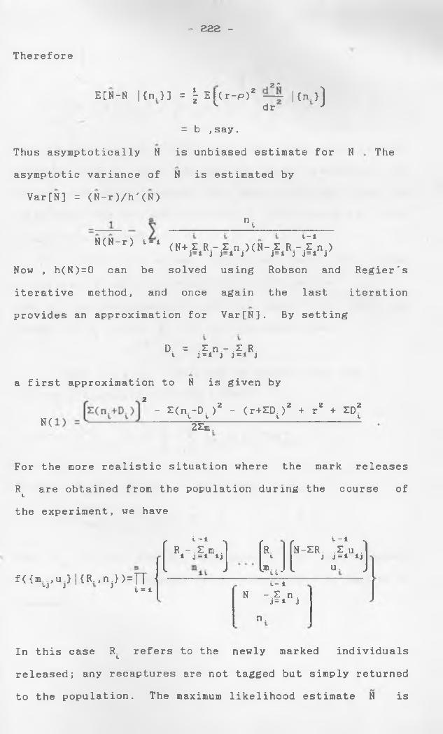
- 222 -

Therefore

2 AE[N-N |{n.}] = \ El(r-p)2 | {rr}]

dr J

= b , say.

Thus asymptotically N is unbiased estimate for N

asymptotic variance of N is estimated by

Var[N] = <N-r)/h'(N)

n .VN(N-r) i=i t-i

The

(N+.ZR-.In.)(N-.IR-.In.)j=i j j=i j j=i j j=i j

Now , h(N)=0 can be solved using Robson and Regier's

iterative method, and once again the last iteration

provides an approximation for Var[N]. By setting

D. = .Z n - .Z R.V J =1 J J=1 J

a first approximation to N is given by2

N(- Z(n -D )z - (r+ZD. )z + rz + ZDz

t t L t

2Zm.

For the more realistic situation where the mark releases

R. are obtained from the population during the course ofithe experiment, we have

f({mij,uj}|{R.,nj}) = TT ■

r i - 1 -x r r i ~ i ^R - .Z m .i j = i ijL J

R.Vjn. ..v u

N-ZR. X u .J J=i ijL u. J

t = 1 t- 1N - X n .

j = i j

n .

In this case R refers to the newly marked individuals

released; any recaptures are not tagged but simply returned

to the population. The maximum likelihood estimate N is

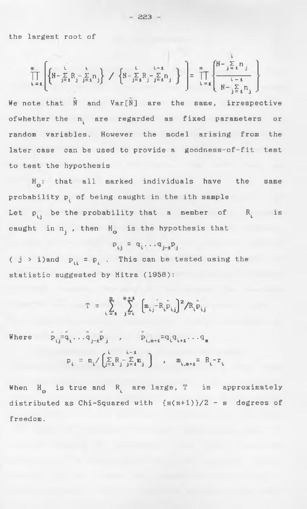
223

the largest root of

r fN- Z n 1

{ N- i Rr i n J / {

r i i - l >N-.Z R.-.Z n.

k j = i j j = i j

s

= TT-i = 1

j = i j

j

i - li N- Z n.k j = i j

ITi = 1

We note that N and Var[N] are the same, irrespective

ofwhether the nt are regarded as fixed parameters or

random variables. However the model arising from the

later case can be used to provide a goodness-of-fit test

to test the hypothesis

H that all marked individuals have the

probability p i of being caught in the ith sample

Let p.. be the probability that a member of R.tj tcaught in n , then Hq is the hypothesis that

p. . = q.. . . q . p.

( j > i)and p u = p . This can be tested using the

statistic suggested by Mitra (1958):

same

is

T = 1 1 hrRAj)zA0t = l j =v

Where p. ,=q. . . . q . d . , p =q.q. „...qIJ 1 J —1 J t,S+l V v + l s

i i - 1

p. = m. / f .Z R.-.Z m. 1 , m. = R.-r.t t ^ J = l J J = 1 J J v , s + l v. t

When H is true and R. are large, T is approximatelyO vdistributed as Chi-Squared with (s(s+l)}/2 - s degrees of

freedom.

224

4.4 CONCLUSIONS

A wide variety of models have been discussed in this

dissertation, and the question now arises as to which

method should be used in a given situation. Obviously the

choice of the method will depend very much on the nature of

the population, its distribution over the population area,

and the method of sampling the population. Where possible,

the experiment should be designed so that more than one

method of estimation can be used.

In the past, little attention has been devoted to the

problem of designing an experiment to yield an estimate

with a given minimum accuracy or precision. For example,

in many of the early applications of the Petersen method,

too few individuals were tagged, so that the number of

recaptures was too small and resulting confidence intervals

too wide. However, for many of the models the variance

formulae are complicated, so that it is not easy to plan

for a given precision. Clearly more research is needed on

the question of design for some methods.

Where possible, the robust but less efficient

regression estimates should be calculated along with more

efficient maximum likelihood estimates. The regression

method is particularly useful when expected values appear

to be correct; but the variances predicted by the model

underlying the maximum-likelihood theory are open to

question because of departures from the underlying

assumptions, for example sampling is not strictly random.

However, in all cases, the assumptions underlying a

particular model should be studied carefully,and where

225

possible appropriate tests carried out. If there is likely

to be any question about the validity of the underlying

assumptions, the sample data should be collected in such a

way that emperical variance estimates are available from

replicated samples. A comparison of the sampling variance

with the estimated theoretical variance predicted by the

model will often throw some light on the validity of the

model.

Of the methods considered in this dissertation the

Petersen method appears to be useful, provided the

assumptions underlying the method are satisfied and there

are sufficient recaptures in the second sample. The main

assumption underlying the Petersen estimate is that marked

and unmarked animals have the same probability of being

caught in the second sample. Unfortunately it is not

always easy to detect departures from this assumption so

that even when all precautions are taken and the assumption

appear to be satisfied, the Petersen estimate may appear to

be biased. If Petersen estimate is to be used extensively

for a given species, then it should be compared with other

estimates and where possible tested on a known population.

If the second sample can be taken in stages then

regression method can be used for testing the assumption

that marked and unmarked animals have the same probability

of capture. The problem of variable catchability may be

overcome by prebaiting, using different sampling methods

for the two samples, changing trap positions etcetera.

However, the most promising approach to the problem is to

avoid recapturing altogether and to obtain an estimate of

the proportion of the marked by simply observing the

226

animals. Tagged animals may also be detected using remote

sensing techniques. If sight records are used then the

second sample is obtained by sampling with replacement and

the binomial model (Bailey ,1952) is applicable.

Sometimes it is not possible to catch enough animals

on the first occasion for a satisfactory application of

Petersen estimate, so that Schnabel method must be used.

In any case the later method should be used if variable is

a problem. Moreover, the schnabel estimate is more

efficient than the Petersen estimate, though the difference

is not great.

It had initially been planned to apply this procedure

to real life data especially on fisheries but my efforts

were fruitless. This was because, most of the models in

literature require well monitored experiments, but the type

of data I got from Kenya Marine and Fisheries Research

Institute (K.M.F.R.I.) lacked this quality. My future goals

are therefore to carry out extensive survey on fisheries

based on well monitored experiments and give applications

of some of the models discussed here. I also hope to

extend my work to open populations.

APPENDIX

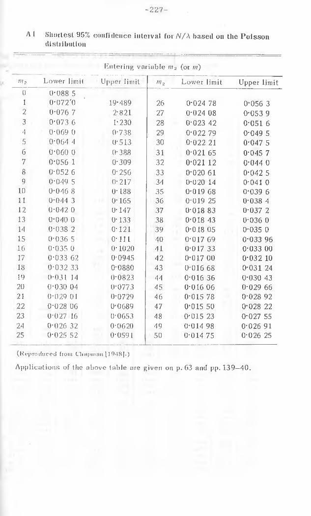
-227-

A l Shortest 95% confidence interval for N /A based on the Poisson distribution

Entering variable m 2 (or //?)w 2 Lower limit Upper limit m 2 Lower limit Upper limit0 0-088 51 0-072'0 ’ 19-4892 0-076 7 2*8213 0-073 6 1-2304 0-069 0 0-7385 0-064 4 0*5136 0-060 0 0-3887 0-056 1 0-3098 0-052 6 0-2569 0-049 5 0-217

10 0-046 8 0- 18811 0-044 3 0-16512 0-042 0 0-14713 0*040 0 0-13314 0-038 2 0 - 1 2 115 0-036 5 0 - 1 1 116 0-035 0 0-102017 0-033 62 0-094518 0-032 33 0-088019 0-031 14 0-082320 0-030 04 0-077321 0-029 01 0-072922 0-028 06 0-068923 0-027 16 0-065324 0-026 32 0-062025 0-025 52 0-0591

26 0-024 78 0-056 327 0-024 08 0-053 928 0*023 42 0-051 629 0-022 79 0-049 530 0-022 21 0-047 531 0-021 65 0-045 732 0-021 12 0-044 033 0-020 61 0-042 534 0-020 14 0-041 035 0-019 68 0-039 636 0-019 25 0-038 437 0*018 83 0-037 238 0-018 43 0-036 039 0-018 05 0-035 040 0-017 69 0-033 9641 0-017 33 0-033 0042 0-017 00 0*032 1043 0-016 68 0-031 2444 0-016 36 0-030 4345 0-016 06 0-029 6646 0-015 78 0*028 9247 0-015 50 0-028 2248 0-015 23 0-027 5549 0-014 98 0-026 9150 0-014 75 0-026 25

( R e p r o d u c e d from C h a p m a n [19 48J . )Applications of the above table are given on p. 63 and pp. 139—40.

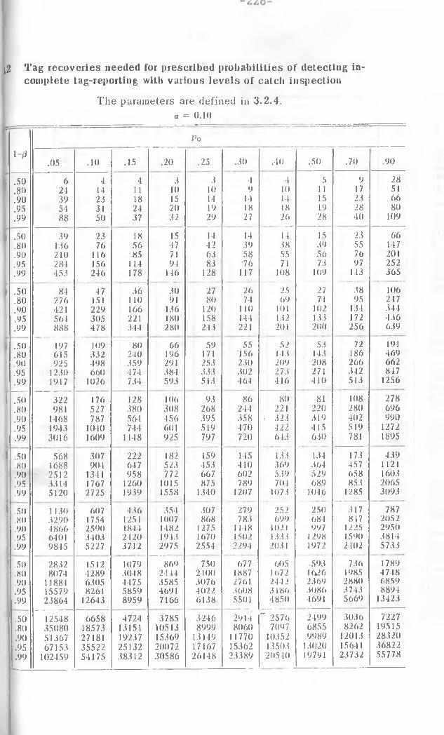
2 Tag recoveries needed for prescribed probabilities of detecting in­complete tag-reporting with various levels of catch inspection

The parameters are defined in 3.2.4.a = 0.10

-Po

1-/3 .90.05 .10 .15 .20 .25 .30 .40 .50 .701 .50 6 4 4 3 3 4 4 5 9 28

.80 24 14 11 10 10 9 10 11 17 51

.90 39 23 18 15 14 14 14 15 23 66

.95 54 31 24 20 19 18 18 19 28 80

.99 88 50 37 32 29 27 26 28 40 109

.50 39 23 18 15 14 14 14 15 23 66

.80 136 76 56 47 42 39 38 39 55 147

.90 210 116 85 71 63 58 55 56 76 201

.95 281 156 1 14 94 83 76 71 73 97 252

.99 453 246 178 146 128 117 108 109 113 365| .50 84 4 7 36 30 27 26 25 27 38 106

.80 276 151 110 91 80 74 69 71 95 247

.90 421 229 166 136 120 110 101 102 134 344

.95 564 305 221 180 158 144 132 133 172 436

.99 888 478 344 280 243 221 201 200 256 639

.50 197 109 80 66 59 55 52 53 72 191

.80 615 332 210 196 171 156 143 143 186 469

.90 925 498 359 291 253 230 209 208 266 662

.95 1230 660 474 384 333 302 273 271 342 847j .99 1917 1026 734 593 513 164 416 410 513 1256[7 5 0 322 176 128 106 93 86 80 81 108 278

.80 981 527 380 308 268 244 221 220 280 696

.90 1468 787 564 456 395 358 • 323 319 402 99095 1943 1040 744 601 519 470 422 415 519 1272

. .99 3016 1609 1148 925 797 720 643 630 781 1895< .50 568 307 222 182 159 145 133 134 173 439

.80 1688 904 647 523 453 410 369 364 457 1121

.90 2512 1341 958 772 667 602 539 529 658 1603

.95 3314 1767 1260 1015 875 789 701 689 853 2065

.99 5120 2725 1939 1558 1340 1207 1073 1046 1285 3093I .50 1130 607 436 354 307 279 252 250 317 787

.80 3290 1754 1251 1007 868 783 699 684 84 7 2052

.90 4866 2590 1844 1482 1275 1 148 1021 997 1225 2950

.95 6401 3403 2420 1943 1670 1502 1333 1298 1590 3814"

9845 5227 3712 2975 2554 2294 2031 1972 2402 5733I .50 2832 1512 1079 869 750 677 605 593 736 1789

.80 8074 4289 3048 2444 2100 1887 1672 1626 1985 4 748

.90 11881 6305 4475 3585 3076 2761 244 2 2369 2880 6859

.95 15579 8261 5859 4691 4022 3608 3 186 3086 3743 8894

.99 23864 12643 8959 7166 6138 5501 4850 4691 5669 13423.50 12548 6658 4724 3785 3246 2914 " 2576 2499 3036 7227.80 35080 18573 13151 10513 8999 8060 7097 6855 8262 19515.90 51367 27181 19237 15369 13119 11770 10352 9989 12013 28320.95 67153 35522 25132 20072 17167 15362 13503 13020 15641 36822.99 102459 54175 38312 30586 26148 23389 20510 19791 23732 55778

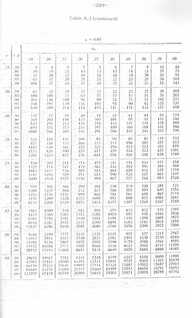
- 2 2 9 -

Table A.2 { c o n tin n e d )

a = 0.05

1-/3

50809095995080<)()95995080909599508090959950809095995080909599508090959950809095995080909599

.05 .10 • .159 6 5

80 19 15•17 28 2268 87 29

101 57 4468 87 29

180 100 75261 1 16 108816 191 110580 289 211187 77 58868 202 118588 2 9 | 212698 876 272

1018 566 409821 178 121827 118 225

1 188 688 •1611521 820 5902281 1228 877

580 289 2111825 711 5151888 101 1 726211 7 1 296 9298600 1921 1 175

985 506 2662289 1227 8808281 1780 12271187 2209 15 786182 8268 22291862 1000 7181178 2888 1 7056287 8850 22878016 •1267 2027

1 1827 6286 •11684666 2 190 1777

11012 5851 116215898 8176 580719572 10886 727128752 152 12 1080820671 10967 778247988 25112 1800066770 25212 2502181619 41776 21689

128797 65478 46219

n0

.20 .25 .30 .40 .50 .70 .905 5 6 7 8 14 46

12 13 13 14 15 25 7519 18 18 18 20 32 9325 23 22 23 25 38 10927 34 33 32 35 51 14325 23 22 23 25 38 10962 57 53 51 54 76 20790 80 75 71 74 102 271

1 16 103 95 90 92 125 331174 153 141 131 133 177 45849 45 42 41 44 63 174

122 109 101 95 97 132 346175 154 142 131 134 178 460224 197 180 166 168 221 566224 291 266 243 244 315 794109 97 90 85 87 119 315266 233 213 196 197 257 653275 327 298 272 272 350 8794 79 417 379 344 343 437 1091710 615 558 503 498 628 1549

174 153 141 131 133 177 458419 364 332 302 301 386 968589 511 464 420 416 528 1310751 651 590 532 525 662 1631

1 1 10 959 867 777 764 953 2328

299 261 239 219 220 285 722712 617 560 505 499 630 1554999 864 781 701 690 863 2114

1272 1098 992 888 872 1084 26411874 1614 1455 1297 1269 1567 3788

582 506 459 415 412 523 12971274 1 185 1070 957 939 1166 28361920 1654 1491 1329 1299 1604 38772111 2100 1891 1682 1641 2018 48592585 3080 2769 2456 2390 2922 7000

1422 1235 1115 997 977 1213 29472240 2871 2582 2291 2230 2730 65444655 3997 3590 3179 3088 3764 89895905 5066 4548 4022 3902 4743 112998651 7415 6649 5870 5684 6886 16345

6224 5348 4799 4243 4116 5000 1190514292 12324 11041 9727 9402 11345 2683019997 17114 15324 13487 13022 15682 2701 125217 2 1660 19389 1 7053 16456 19791 4665236989 31632 28303 24871 23978 28788 67742

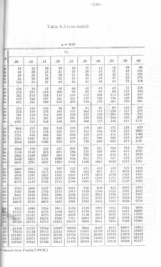
-230-

Table A. 2 (c o n c l u d e d )

a = 0.01

P 0

'P .05 .10 .15 .20 .25 .30 .40 .50 .70 .90

50 17 12 10 10 10 11 13 16 28 9250 45 28 23 21 20 20 22 25 42 131JO 65 39 31 28 27 26 28 32 51 15595 84 50 39 35 33 32 33 37 59 17599 126 73 57 49 46 44 45 49 75 218V—50 126 73 57 49 46 44 45 49 75 21880 278 157 118 100 90 85 83 88 127 35090 382 213 158 133 119 112 108 113 159 43295 479 266 197 164 147 137 130 136 188 50699 692 381 280 232 205 190 179 184 250 661

50 271 154 116 98 89 84 82 87 125 31780 578 319 235 195 174 162 153 158 217 57990 781 428 314 259 230 212 199 204 276 723.95 971 531 387 319 281 259 242 246 329 855.99 1385 75 3 546 448 393 360 332 336 441 1131

ST 648 357 262 218 193 179 169 174 238 629.80 1312 713 518 425 373 342 316 320 422 1083.90 1751 948 686 561 490 449 412 414 539 1368.95 2162 1167 843 687 599 54 7 500 500 645 1629.99 3048 1640 1180 959 834 758 688 685 874 2181

:5 o 1060 578 422 347 305 281 261 266 353 91480 2110 1140 823 671 586 535 489 490 633 159790 2802 1509 1087 883 769 700 636 634 811 202995 3446 1852 1331 1080 938 852 772 767 975 242499 4835 2591 1857 1503 1302 1180 1063 1050 1323 3261

50 1869 1011 732 597 522 477 437 439 570 144480 3661 1966 1413 1145 994 903 817 81 1 1029 255590 4834 2591 1857 1502 1301 1179 1063 1050 1323 326195 5927 3172 2270 1834 1586 1435 1290 1271 1593 390999 8775 4419 3156 2544 2196 1984 1775 1743 2169 5282

50 3724 2000 1437 1 165 1011 918 830 824 1045 259380 7184 3840 2744 2214 1913 1729 1550 1524 1902 464790 9441 5038 3595 2896 2498 2255 2015 1976 2152 595795 11537 6150 4383 3528 3040 2741 2445 2393 2958 716199 16035 8534 6074 4882 4201 3782 3364 3283 4036 9719

50 9332 4980 3554 2863 2470 2229 1993 1954 2424 589480 17752 9444 6720 5398 4643 4178 3714 3621 , 4445 1068990 23221 12342 8773 7040 6049 5438 4824 4695 5742 1375995 28291 15027 10674 8560 7351 6604 5851 5687 6938 1658699 39150 20774 14743 11812 10134 9096 8044 7804 9488 22601

50 41348 21937 15566 12469 10696 9600 -8487 8232 10002 2381380 77628 41128 29142 23312 19969 17897 15779 15263 18444 4368290 101102 53539 37919 30318 25958 23254 20483 19795 23878 5644895 122823 65021 46037 36797 31496 28206 24830 23981 28893 6822399 169262 89565 63386 50642 43326 38784 34111 32916 39588 93317

' tot luced from P a u l i k [1 9 6 11 . )

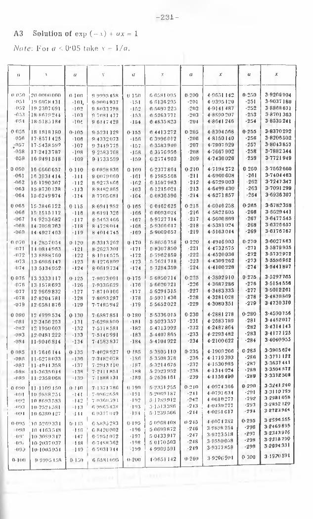
- 231-

A3 Solution of exp (-a) ax - 1

Note: For a < 0*05 take v - 1 /a .

a .V a V a X a X a X

o or.o 20 OOOO 000 0 ino 9 9995 458 0 150 6 6581 095 0 200 4 0051 142 0 250 3 9206004or. i 19 6078 431 •101, 9 9004 937 151 0 6136295 •201 4 9395120 •251 3 9037 180or.2 19 2307 691 102 9 8033 798 •152 0 5697 225 202 4-9141 487 •252 3 8808671

•053 18 6679244 103 9 7081477 1 53 0 5263 771 •203 4 8SP0207 •253 3 8701 303or. i 18 5185184 •10* P 6147 420 •154 0 4835823 •204 48641246 •254 3 8535241

0 055 18 1818180 0 105 9 5231129 0 155 0 4413272 0 205 4 8394 508 0 255 3 8370 292058 17-8571 4 25 •106 9 4332073 • 150 0 3996 012 •200 4 8150140 •250 3 8206502•057 17-5438592 •107 9 34 49775 157 0 3583 940 •207 4-7907 929 •257 3 8043857•058 17 2413787 108 9 2583 768 •158 6 3170950 •208 4-7607 902 •258 3-7882 344•059 16 9491518 •109 9 1733599 •159 G 2774 902 ■209 4-7430026 •259 3-7721 949

0 060 16 0666657 0 110 9 0898836 0 100 G 2377 804 0 210 4 7194 272 0 2G0 3-7562060•061 16 3934 414 •111 9 0079060 101 6 1985508 211 4 0900608 •261 3-7404 463•062 16 1290307 112 8 9273 866 •162 0 1597 983 •212 4 6729003 •202 3-7247347•063 15 8730138 •113 8-8482865 •163 0 1215021 •213 4 6499430 •263 3-7091299•004 15 6249974 -114 8 7705G81 •104 0 0830590 •214 4 6271 857 •264 3 6936 307

0 005 15-3840 122 0 115 8 6941 952 0 105 0 0102625 0 215 4 6046258 0 205 3 6782358066 15 1515112 •116 8 6191 320 •166 0 0093024 •216 4 5822G05 •266 3 6629441•067 14 9253 682 •117 8-5453 466 •167 5 9727714 •217 4-5600869 •207 3 6477545•068 14 7058763 •118 8 4728044 •108 5-9360 617 •218 4 5381024 •2G8 3 0320057■069 14 4927 463 •119 8 4014 745 •169 5 9009657 •219 4 5163014 •269 3 0170767

0 070 14 2857 054 0 120 8 3313262 0 170 5 8650 758 0 220 4 4946903 0 270 3 0027 863•071 1 4 0844 903 121 8-2623 301 •171 5 8307 850 •221 4 4732575 •271 3 5879935•072 13 8888 760 •122 8 194 4 575 •172 5-7902859 •222 4-4520036 •272 3 5732972073 13 6986 147 •123 8 1276809 •173 5 7021 718 •223 4 4309262 •273 3 5580902074 13 5134952 •124 8 0619 734 174 5 7284 359 •224 4-4100228 •274 3 5441 807

0 075 13 3333 117 0 125 7-9973091 0175 5 G950714 0-225 4-3892910 0-275 3-5297 705•076 13 1578693 •126 7-9336 629 •176 5 0620721 •226 4 3687 286 •276 3 5154 556•077 12 9809 832 •127 7 8710106 •177 5 6294 315 •227 4 3483333 •277 3 5012201•078 12 8204 781 •128 7 8093 287 •178 5 5971430 •228 4 3281028 •278 3-4870869•079 12 6581876 •129 7-7485942 •179 5 5652022 •229 4 3080351 •279 3 4730370

0 080 12 4999534 0 130 7G887 851 0 180 5-5336015 0 230 4-2881 278 0-280 3-4590756•081 12 3456 253 •131 7-6298 800 •181 5 5023 357 •231 4-2083789 •281 3 4452017•082 12 1950603 •132 7-5718581 ■182 5 4713992 •232 4-2487 864 •282 3 4314 143•083 12 0481 222 •133 7-5146991 •183 5 4407 865 •233 4-2293 482 •283 3 4177 125•084 11-9046814 •134 7-4583837 •184 5 4104 922 •234 4-2100622 •284 3 4040953

0 085 1 1-7646 144 0 135 7-4028927 0 185 5 3805 110 0 235 4-1909 2G0 0-285 3 3905 624•086 1 1-6278 033 •136 7 3482078 •180 5 3508 378 •230 4 1719393 •280 3-3771 122•087 1 1 4941358 •137 7 2943 1 10 •187 5 3214 075 •237 4 1530 985 •287 3 3637 441•088 11 -3035044 •138 7-2 4 1 1 851 188 5 2923 952 •238 4 1314 024 •288 3 3504 572•089 1 1 2358 068 • 139 7 1888131 •189 5 2630101 •239 4 1158400 •289 3-3372 508

0 090 11 1 109 150 0140 7 1371786 0 190 5 2351255 0 240 4 0974 300 0 290 3 3241 240•091 10 PSSR25I •141 7-0862 658 •191 5 2009187 •241 4 0791031 •291 3 31 10759• 092 10 8693 583 •142 7 0360 593 192 5 I7S99I2 •°4 2 4-OG10277 •292 3 2981058•093 10 7521581 •143 6 9865 4 38 • 193 5 1513386 •243 4 0430277 •293 3 2852 129

1 094 10-6380 427 111 6 9377 0 49 194 5 1 239566 •214 4 0251617 •294 3 2723964

0 095 10 5260 331 0 l 15 6 8895 283 0 195 5 0908408 0 245 1 0074 2S2 0 295 3 2594555 3 2469895 3 2343 976 3 2218 790 3 2094331

•090•09'

10 416354810 3089 3 47

116147

G 8420002 0-7951 072

•196•197

5 0699872 5 0433 917

•246•247

3 9898 254 3 9723 518

•296•297

•09/•099

10 2037 037 10 1005954

118149

0-7488 362 6 7031 744

•198•199

5 0170503 4 9909591

•248•249

3 9550058 3-9377858

•298•299

0-100 9 9995 458 0 150 6 6581095 0 200 4-9651 142 0 260 3-9206 901 0 300 3 1970 591

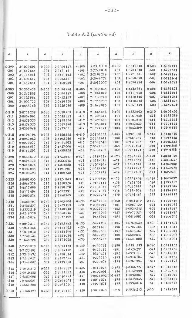
- 232-

Table A.3 ( c o n t i n u e d )

a X a X u X a X a X

' 0 300 3-1970 591 0 350 2 6506127 0 400 2 2316119 0 450 1 8847348 0 500 1-5936243•301 3 1847564 •351 2 0471 41 1 •401 2 2240010 •451 1-8784240 •501 1 5882633

1 -302 3 1725241 •352 2 0377 143 •402 2 2104218 •452 1 8721351 •502 1 5829188•303 31G03G17 •353 2-0283321 •403 2-2088724 •453 1-8658679 •503 1-5775904•304 3 1482684 •354 2 0189 939 •404 2 2013532 •454 1 8596224 •504 1-5722783

0 305 313G2436 0 355 2 0090 990 0 405 2 1938638 0 455 1 8533984 0 503 1-5669623•300 3 12428G6 •356 2-0004 487 •406 2 1864042 •450 1 8471 958 •506 1 5617022•307 3 1123968 •357 2 5912 409 •407 21789740 •457 1 8410145 •507 1-5564 38!•308 3 1005735 •358 2-5820758 •408 21715732 •458 1 8348542 •508 1-5511898•309 3-0888160 •359 2-5729 530 •409 2 1642015 •459 1 8287149 •509 1-5450572

0 310 3 0771 238 0 300 2-5038723 0 410 215C3580 0 4C0 1 8225905 0 510 1 5407 403•311 3-OG54 9G1 •361 2 5548333 -411 2 1495444 •461 1 8164989 •511 1 5365389•312 3 0539325 •302 2-5458 356 •412 21422588 •462 1 8104218 •512 1-5303 53!313 3 0424 323 •303 2-5368790 -413 2 1350014 •403 1 8043652 •513 1 5251820•314 3 0309949 •364 2 5279631 •414 2 1277721 •464 1-7083 290 •514 1 5200276

0 315 3 0196198 0 305 2-5190875 0 415 2 1205707 0 465 1 7923131 0 515 1-5148876•316 3 0083 002 •306 2 5102520 •410 2 1 133 971 •466 1 7*63172 •516 1 5097628317 2 9970 537 •367 2 5014 563 •417 2 1002510 •407 1 7603413 •517 1 5046532•318 2-9658 017 •368 2-4927 000 •418 2 0991 322 •463 1 7743854 •519 | -4995 6*5319 2 9747297 •369 2-4839828 •419 2 0920 406 •469 l 7684491 •519 1 4944788

0 320 2 9G3G570 0 370 2 4753044 0 420 2 0849 750 0 4 70 1-7625325 0-520 1 4894139•321 2-9526 432 •371 2 4006045 •421 2 0779381 •471 1 7566 355 •521 1 4*43637•322 2 9410876 •372 2 4580 629 •422 2 0709268 •472 1 7507 573 •521 1-4793282•323 2-9307 898 •373 2 4 494 991 •423 2 0039420 •473 1 74 49 995 •523 1-4743 074•324 2 9199493 •374 2 4409730 •424 2 0509 834 •474 1 7390603 •524 1-4693011

0-325 2 9091 655 0 375 2 4324 843 0 425 2 0500 510 0 475 1 7332402 0 525 1-464 3092•326 2-8964 379 •376 2 4240326 •420 2 0431444 •470 1 7274391 •526 1 4593317•327 2-8877 060 •377 2 4150176 •427 2 0302035 •477 1 7210 56ft •527 1-4543686•328 2-8771 494 •378 2 4072391 •428 2 0291083 •478 1 7163932 •528 1 4494195•329 2-8005874 •379 2-3988 909 •429 2 0225 784 •479 17101 483 •529 1 4444847

0 330 2-8500 797 0 3S0 2-3905 900 0 4 30 2 0157 738 0 430 1-7044219 0 530 1-4395640•331 2-8456257 •381 2-3823 199 •431 2 0089 942 •4S1 1 6987139 •531 1-4346573•332 2 8352249 •3S2 2-3740846 •432 2 0022 395 -482 1 6930242 •532 1 4297645•333 2 8248 770 -383 2-3G68 845 •433 1-9955 095 •4S3 1 6873 527 •533 1-4243856•334 2 8145814 •384 2 3577192 •431 1-9838042 •484 1 6816993 •534 1-4200 205

0 335 2 8043 377 0 385 2-3495885 0 435 1-9821 232 0 485 1 6760639 0 535 1-4151691•336 2-7941 455 •3S6 2 3414 922 •436 1-9754 665 •4S0 1-6704464 •536 1 4103313•337 2-7840042 •387 2-3334 300 •437 I-9GS3339 •437 1 6GI8467 •537 1-4055072•338 2-7739134 •388 2 3254 016 •438 1 9622 253 •483 1 6592647 •538 1-4006965•339 2-7638 728 •389 2 3174068 •439 1-9550 405 •489 i 6537 002 •539 1-39589940 340 2*7538 818 0 390 2 3094 453 0 440 1-9400 792 0 490 1 6481533 0-540 1-3911 155•341 2-7439401 •391 2 3015170 •441 1 9425415 •491 1 6426 237 •541 1-3863 450•342 2 7340472 •392 2 2936214 ■442 1-9360271 •492 1 6371 ill •542 1-3815878•343 2 7242027 •393 2-2857 5.85 443 1-9295360 •493 1 6316164 •543 1 -3768437314 2-7144062 •394 2 27792SO 444 1 9230678 •494 1 6201384 •514 1-3721 128

0-345 2 7016573 0 395 2 2701 297 0 445 1-9166 226 0-495 1 6206774 0 545 1-3673 946•316 2 0949555 •396 2-2023 632 •446 1 9102001 •496 1 6152333 •516 1-3620 899•347 2 6853000 •397 2 2546 264 447 l-903800£ 54-*97 1 6098 061 •517 1-3579 979•318 2 6756921 •398 2 2409251 •448 1 8974 228 -498 1 Go 13955 •518 l 3533187•319 2 OGGI 290 •399 2 2392 530 •419 1 891067? •499 1-5990016 •519 1-3466 ;>23

0 350 2 6566127 0 400 2 2310 119 0 450 1S81734S 0 500 1-5936 243 0-550 1-3439987

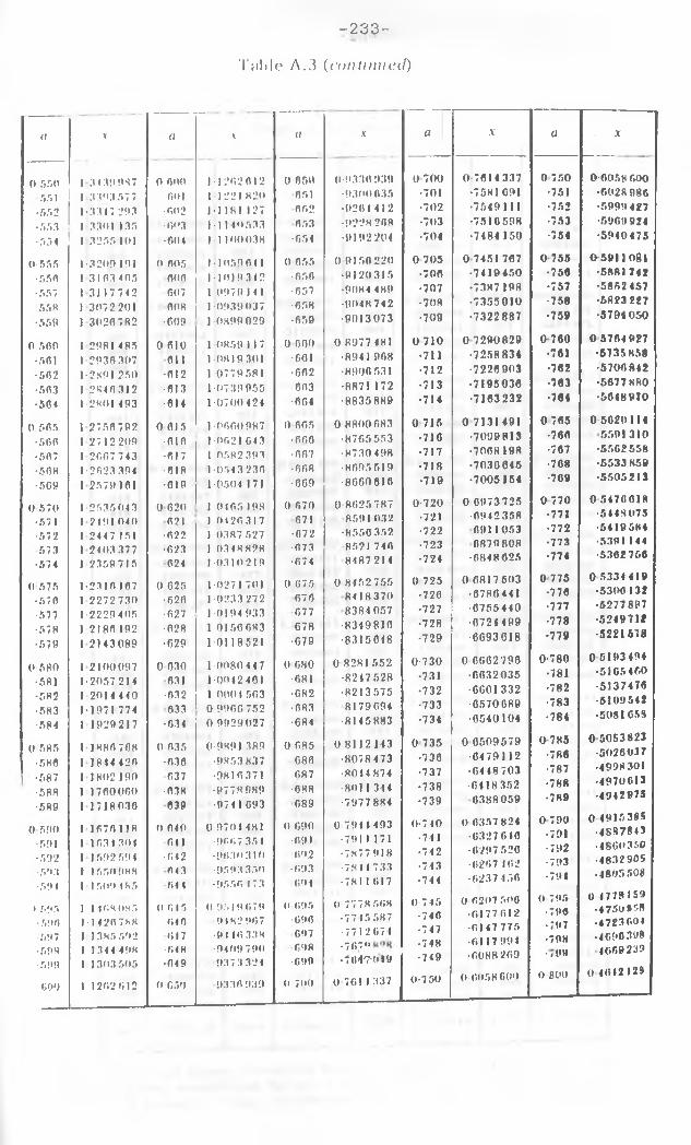
-233-Tfible A .3 {continued)

a V (l X

0 550 1 3139987 0 0«HI 1 1202 012551 1 3393577 •601 1 1221 H20•552 1-3347 293 -002 M 181127•653 1 3301 J35 •IW*3 j 1140533•554 I 3255101 •604 1 1100038

0-555 1-3209 191 0 005 1-1059 041•550 1 3163405 ooo 1-1019 3*2•r».s7 13117742 607 1 0979 1 4 155 R 1 3072201 008 1 0939037•559 1 3026782 ■609 1 0H99029

0 500 1 2981485 0 610 1 0859 1 17•501 1 2936 307 O il 10819301•502 1-2S91 250 -012 1 0779581•503 1 2840312 •613 10739 955•564 1-2K01 493 -614 1 0700424

0 605 1 2756792 0 015 10000 987•600 1 2712 209 -010 1 0021043•507 1 2007743 •017 10582 393•508 1-2023 394 -618 1 0543230•609 1 2579161 -019 1-0504 171

0 570 1 2535043 0 620 1 0405198•571 1 2491 040 021 J 0420317•57 2 1 2447151 •022 1-0387 527573 1 2403377 •623 J 0348828•574 1 2359715 024 1 0310219

0 575 1-2310 167 0 625 1-0271 701•670 1 2272730 •620 1 0233 272■577 1-2229406 ■627 1 0194 933•678 1 2180192 •028 1 0150083•579 1 2143089 •G29 1 0118 521

0-580 1 2100 097 0 030 1 0080447•581 1-2057 214 631 1 0042401•582 1 2014440 ■032 1 0004503•583 1-1971 774 633 0 9906 752•584 1 1929217 •634 0 9929027

0 585 11880708 0 635 0 9891 389•680 1 18 44 420 •636 •9853837•587 1 1802190 037 •9810 371•588 1 1760060 ■038 9778989•589 11718030 039 •9741G93

0 590 1 1070 1 18 0 040 0 9701481•691 1 1034304 641 9007354•592 1 1592594 •642 •9630310•593 1-1550 9HH 043 9593350•591 I 1609485 04 4 •9550473

* 595 1 )4 6 8 0 8 5 0 015 0 9519679•596 M420788 040 9182907•697 1 1385592 047 •9116 338•598 1 1344498 ■04 8 -9409790•599 I 1303505 -049 937 3 324600 1 1202 012 (l 050 9330 939

a X a .V a

0 050 0 9330939 0 700 0 7014 337 0 750051 •9300635 •701 •7581091 •751052 •9264 412 •702 •7549 III •752053 •9228 268 •703 •7510 598 •753•054 9192204 •704 •7484 150 •754

0 055 0 9150 220 0 705 0 7451 707 0 755•650 •9120315 •700 •7410450 •756•057 •9084 489 •707 •7387 198 •757-058 •9048742 •708 •7355 010 •758•059 •9013073 •709 •7322887 •759

0 000 0 8977 481 0 710 0 7290629 0 760•001 •8941908 •711 •7258834 •701•002 •8906531 •712 •7226003 •762003 •8871 172 •713 •7195036 •703•004 •8835889 •714 •7103232 •704

0 065 0 8800 683 0 715 0 7131 491 0 705•000 •8705 553 •710 •7099813 •700•007 •8730498 •717 •7008 198 •707•008 •8095 519 •718 •7030045 •708•0G9 ■8000 810 •719 •7005154 •700

0 070 0 8625 787 0-720 0 0973725 0 770071 8591032 •721 •0942 358 •771•072 ■8550 352 •722 0911053 •772•073 8521746 •723 0R79R0R •773•074 8487 214 •724 •0848 025 •774

0 075 0 8452 755 0 725 0 0817 503 0 775070 8418370 •720 •0780441 •770077 8384057 •727 •0755440 •777678 •8349816 •728 •0724499 •778•G79 •8315048 •729 •6093 618 •779

0 080 0 8281552 0-730 0 GG02790 0-780•081 •8247 528 •731 •0632035 •781•082 •8213575 •732 ■GG01332 •782■083 8179694 •733 •6570 089 •783•684 •8145883 •734 •6540104 •784

0 085 0 8112143 0 735 0 0509579 0 785080 •8078 473 •730 •6479112 •786087 •8014 874 •737 •6448703 •787■088 8011344 •738 •6418 352 •788089 •7977 884 •739 6388059 •789

0 090 0 794 4493 0-7 40 0 0357 824 0 790•091 •7911 171 •741 •6327 640 •791092 •7877918 •742 •0297 520 •792• 093 •7911733 •743 •0207 462 •793694 •7811617 •744 •0237450 •794

(1095 0 7778568 0 745 0 6207 500 0 795•696 •7715 587 •740 •0177012 •700697 •771 267 1 •747 •01 4 7 775 •797098 •767" •748 •6117 994 •798•G90 •704'TOf9 •749 •0088209 • i Mil

0 700 0 7GI1337 0-750 0-6058 600 o goo

x

o-oo.r,8 0oo•602ft986 •6999 4 27 •6969 924 •5940475

0-5911 Of) | •SftRl742 •5862 457 •6823 227 •5791060

0 5764 927 •5735 858 •5706842 •5677 880 •5048970

0 5620 II4 5591 310 •5562558 •5533 859 •5505 213

0 5470018 •5449073 •6419584 •5391 144 •5302 760

0 5334419•5300132•5277897•5249712•5221578

0 5193494 •5165460 •5137470 •5109542 •508165S

0 5053823 •5026037 •4998301 •4970613 •4942975

0 4915385• 4887843• 4660350 •4832 905• 4 805508

0 1779 159 •4750958• 4723601• 4690398 4609239

0 4642 129

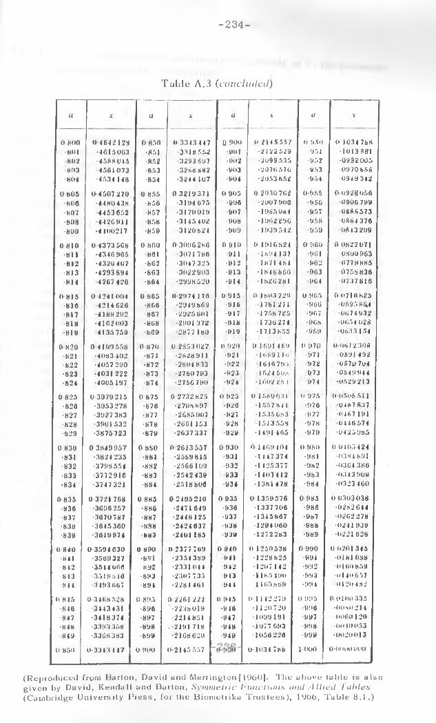
- 234-

Table A.3 (c o n c lu d e d )

(i X u X

0 800 0 4642128 0 850 0 3313 117801 •4615003 •851 3318 652802 4588015 852 •3293 697•803 4561073 853 •3268 882804 4534 148 -854 •3244 107

0 805 0 4507 270 0 855 0 3219371•806 •44HO 438 •850 •3194 675•807 4453652 857 •3170019■808 •44 20 911 •858 •3145 402•809 •4400217 •859 3120824

0 810 0 4373508 0 800 0 309G2SG■811 •4340 905 •861 •3071780812 •4320407 •862 •3017 325813 •4293 894 •863 •3022903814 •4267 420 •864 •2998520

0 815 0 4241 004 0 805 0 2974170-810 4214620 •800 •2949 869•817 •4188292 •807 •2925 001•818 •4102003 •808 •2901372•819 4135759 •b09 •2877180

0 820 0 4109558 0 870 0 2853027•821 •4083 402 •871 •2S28911•822 •4057 290 •872 •2801833•823 •4031222 •873 •2780793•824 •4005197 •874 •2756 790

0 825 0 3979215 0 875 0 2732 625•820 •3953 278 •870 •2708 897•827 •3927 383 •877 •2685007■828 •3901532 •878 •2001153•829 •3875723 •879 •2037 337

0 830 0 3849957 0 8S0 0 2613557•831 •3824 235 •881 •2569 815•832 •3798 554 •882 •2506109•833 •3772910 •883 •2542439•834 •3747 321 •884 •2518 606

0 835 0 3721768 0 885 0 2495210836 •3690 257 •886 •2471649837 •3070787 •887 •2448125•838 •3045 360 •898 •2424037•839 •3019974 •883 •2401185

0 840 0 3594 030 0 890 0 2377709•HI 1 •3509 327 •891 -2354 389812 •3514 000 K92 •2331014813 3518840 •893 •2307 735841 3493 007 •891 •2281401

0 815 0 3108 528 0 895 0 2261 222•816 3143431 ■896 •2238019•847 •3418374 •897 •2214 851•818 •3393358 •898 •2191718849 •3308 383 •899 •2168 620

0 850 0-3313 117 0-900 0-2145 557

u X a V

0 900 0 2145557 0 950 0 1034 7bH•901 •2122129 951 •1013381•902 •2099 535 •952 •0992005•903 •2070 576 653 0970656904 •2053 652 954 0949342

0 905 0 2030702 0-955 0 0928056•906 •2007 900 •950 0906799907 •1985064 •957 •0685573•908 •1902296 •958 0864376■909 •1939542 •959 (1643 209

0 910 0 1916824 0 900 0 0822071911 •1694137 •901 0S00963-912 1871484 •962 •0779885•613 •184 8 660 •963 •0758 836-914 •1620281 ■964 •0737 610

0 915 0 1603729 0 965 0 0710 825•616 1761211 •900 •0695 864•617 •1758 725 •967 •0074 932•918 •1730 274 •908 •0654028•919 •1713655 •969 •0033154

0-920 0 1091469 0 97() 00012 308•921 -1069 1 10 971 ■0591492•922 1610 79 > 972 •0570 704•923 1024 50.n 973 •054 9 94 4•924 •100225 i U74 •0529 213

0 925 01580031 <* 975 0-050S5I 1•920 •1557841 •976 •0487 837•927 •1535 683 •977 •0407191•628 •1513 558 •978 •0140574•629 •1491405 •979 •04 25 985

0 930 0 1409104 0 9S0 0 0 405424931 •1 4 47 374 •981 •03.84 691•932 •1425 377 •982 •0304 366•633 •1403412 •963 •03 4 3 909934 •1381478 •984 •0323400

0 935 0 1359576 0 985 0 0303 038•936 •1337706 •986 •0282644•937 •1315867 •967 •0262 278■938 •1291060 •688 •0241939■639 •1272283 •989 •0221628

0 910 0 1250538 0 990 0 0201 345911 •1228825 •991 -0181088942 •1207 142 •992 •0160 859913 •1185190 •993 •o| 4**657911 •1103809 •99 4 •0120 492

(t 945 0 1 142 279 0-995 0 0100 335■916 •1120720 •996 •Oo>u 214•947 •1099191 •997 (1060 120■948 •1077 693 •998 •0o 10053■949 1056 226 •999 •0020013

01034786 1-000 0-0ot *0 4*1*0

( R e p r o d u c e d from B a r t o n , D a v i d a n d M er r i n g t o n 11960). T h e a b o v e t a b l e is a l s o g i v e n by D a v i d , K e n d a l l a n d B a r t o n , Sy mme tr ic Inunct ions ami A l l i e d l a h l e s ( C a m b r i d g e U n i v e r s i t y P r e s s , for t h e B i o m e t r i k a T r u s t e e s ) , 1966 , T a b l e 8 . 1 . )

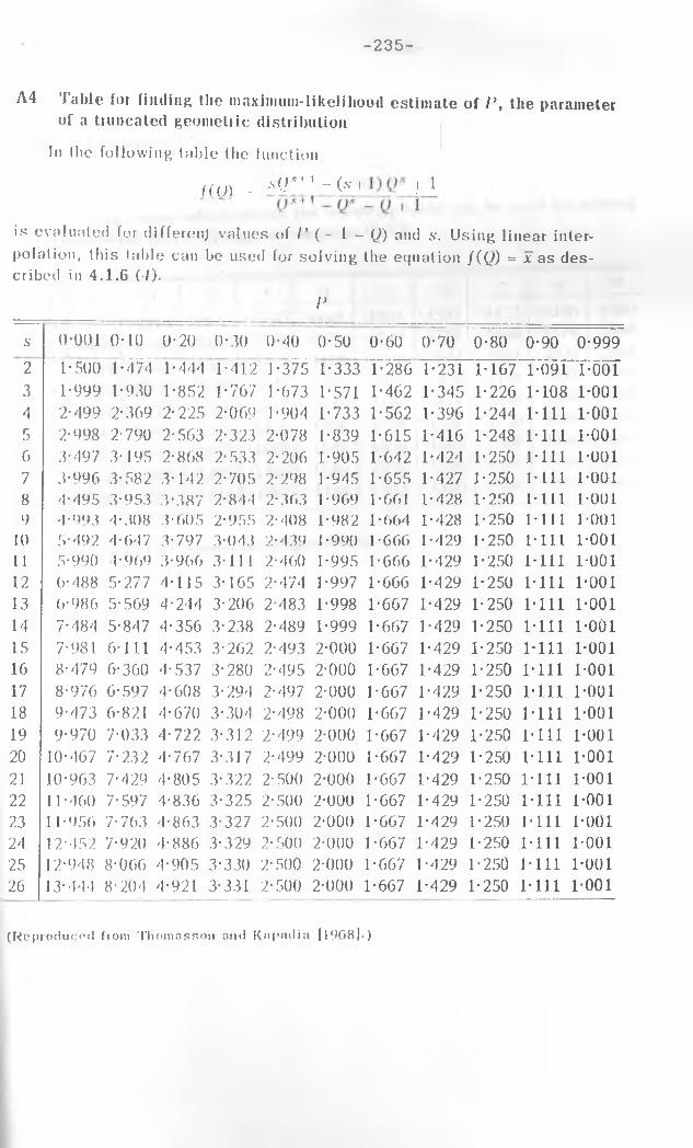
- 235-

A4 Table for finding the maximum-likelihood estimate of P , the parameter of a truncated geometric distribution

In (he following table the function

K O ) - •s<-r+1 - ( * ■ ' 1

is evaluated for differenj values of /’ (- 1 — (1) and 5. Using linear inter­polation, this table can be used for solving the equation f ( Q ) = x as des­cribed in 4.1.6 (4).

P

s 0-001 0* 10 0-20 0*30 0-40 0-50 0-60 0-70 0-80 0-90 0-9992 1-500 1*474 1*444 1-412 1-375 1-333 1-286 1-231 1-167 1-091 1-0013 1-999 1*930 1-852 1*767 1-673 1-571 1-462 1-345 1*226 1-108 1-0014 2-499 2-369 2-225 2-069 1-904 1-733 1-562 1-396 1-244 M i l 1-0015 2-998 2-790 2-563 2-323 2-078 1-839 1-615 1-416 1-248 1-111 1-0016 3-497 3-195 2*868 2*533 2-206 1-905 1-642 1*424 1-250 1-111 1-0017 3-996 3-582 3-142 2-705 2-298 1-945 1-655 1-427 1-250 1-111 1-0018 4-495 3-953 3*387 2-844 2-363 1*969 1*661 1-428 1-250 1*111 1-0019 4-993 4-308 3-605 2-955 2-408 1-982 1*664 1-428 1-250 1-111 1-00110 5-492 4-647 3*797 3-043 2-439 1-990 1*666 1-429 1-250 1-111 1-00111 5-990 1-969 3-966 3-111 2-460 1*995 1-666 1-429 1-250 1-111 1-00112 6-488 5*277 4-115 3-165 2-474 1-997 1-666 1-429 1-250 1-111 1-00113 6-986 5-569 4-244 3-206 2-483 1-998 1-667 1-429 1-250 1-111 1-00114 7-484 5-847 4-356 3-238 2-489 1-999 1-667 1-429 1-250 1-111 1*00115 7-981 6-111 4-453 3-262 2-493 2-000 1-667 1-429 1-250 1-111 1-00116 8-479 0-300 4*537 3- 280 2*495 2-000 1-667 1-429 1-250 1-111 1-00117 8-976 6-597 4-608 3*294 2-497 2-000 1-667 1-429 1-250 1-111 1-00118 9-473 6-821 4-670 3-304 2-498 2-000 1-667 1-429 1-250 1-111 1-00119 9-970 7-033 4-722 3-312 2*499 2-000 1-667 1-429 1-250 1-111 1*00120 10-467 7*232 4-767 3-317 2*499 2-000 1-667 1-429 1-250 1-111 1-00121 10-963 7-429 4-805 3*322 2-500 2-000 1-667 1-429 1-250 1-111 1-00122 11-460 7-597 4-836 3*325 2-500 2-000 1-667 1-429 1-250 1-111 1-00123 11*956 7*763 4-863 3-327 2-500 2-000 1-667 1-429 1-250 1-111 1-00124 12*452 7*920 4-886 3*329 2*500 2-000 1-667 1*429 1-250 1-111 1-00125 12-948 8-066 4-905 3*330 2-500 2-000 1-667 1-429 1-250 1-111 1-00126 13*444 8-204 4-921 3-331 2-500 2-000 1-667 1-429 1-250 1-111 1-001

( R e p r o d u c e d fiom T h o m a s s o n a n d Ks ip ad ia 119G8J.)

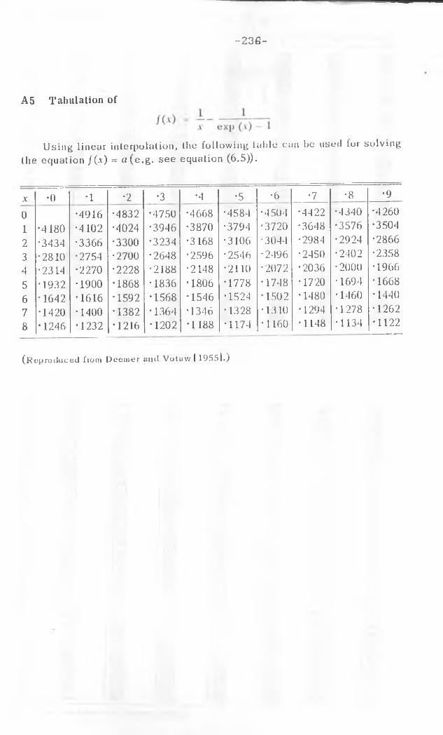
- 236-

A5 Tabulation of

Using linear interpolation, the following table can be used for solving the equation /(a) = «(e.g. see equation (6.5)).

X •0 •l •2 •3 •4 •5 •6 •7 •8 •90 •4916 •4832 •4750 •4668 •4584 •4504 •4422 •4340 •4 2601 •4180 •4102 •4024 •3946 •3870 •3794 •3720 •3648 •3576 •35042 •3434 •3366 •3300 •3234 •3168 •3106 •3044 •2984 •2924 •28663 •2810 •2754 •2700 •2648 •2596 •2546 •2496 •2450 •2402 •23584 •2314 •2270 •2228 •2188 •2148 •2110 •2072 •2036 •2000 •19665 •1932 •1900 •1868 •1836 •1806 •1778 •1748 •1720 •1694 •16686 •1642 •1616 •1592 •1568 •1546 •1524 •1502 •1480 •1460 •14407 •1420 •1400 •1382 •1364 •1346 •1328 •1310 •1294 •1278 •12628 *1246 •1232 •1216 •1202 •1188 •1174 • 1160 •1148 •1134 •1122

( R e p r o d u c e d from D e e m e r a n d Votuvv I 1 9 5 5 b )

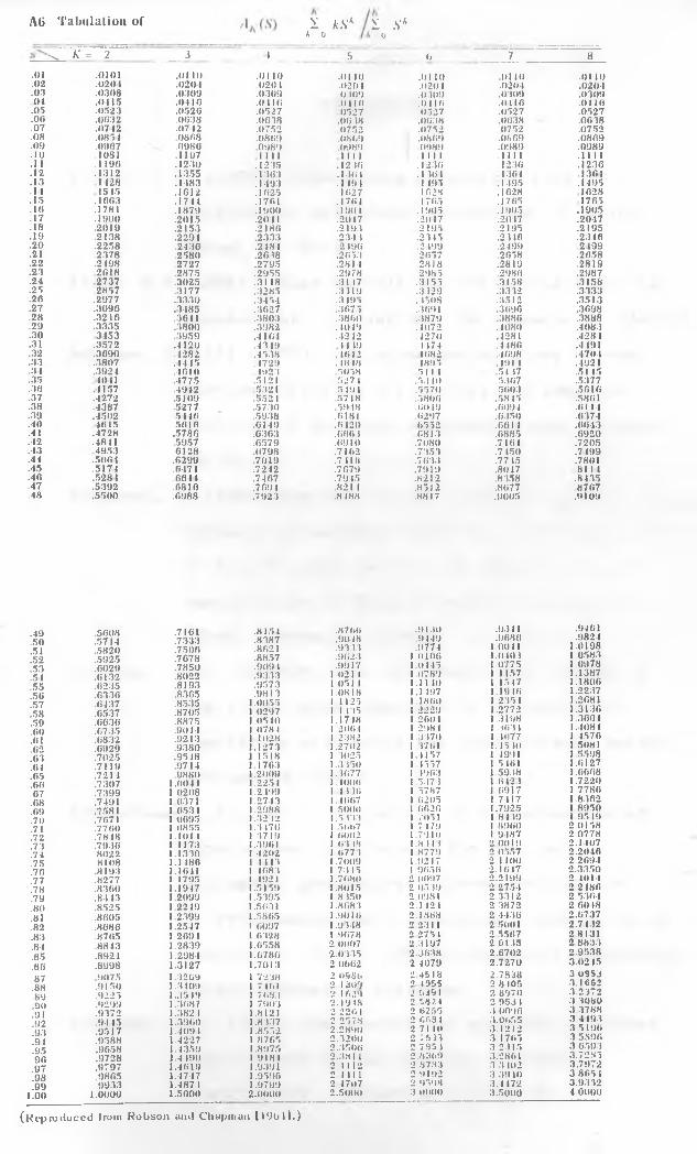
AG Tabulation of X kSk \ SKa g o^ K = 2 3 1 .5 6 7 8

.01 .0101 .01 10 .01 10 .01 10 .01 10 .0111) .01 10.02 .0201 .0201 .020 1 .0201 .0201 .0204 .0204.01 .0.308 .0309 .0309 .0309 0)09 .0309 .030901 .0115 .0110 .0110 (II10 .0110 .0410 .0110.05 .0523 .0520 .0527 0527 .0527 .0527 .0527.00 .0032 .0038 .0038 .0038 .0038 .0038 .0038.07 .0712 .07 12 .0752 (1752 0752 0752 .0752.08 .085 1 .0808 .0809 .0809 0809 .0809 .0809.0!) .0967 .0980 .0989 .0989 .0989 .0989 .0989.10 .1081 .1107 1 II 1 111) 1111 .1111 .1111.1 1 .1190 .1230 .1235 .1230 . 1230 . 1230 .1230.12 .1312 .1.355 .1363 .1301 . 1 Hi 4 1304 . 1301.13 .1 128 .1483 .1493 .1 19 1 1 195 .1495 .1495.11 1515 .1012 . 1025 .1027 1028 .1028 1028.15 . 1 003 .1711 .1701 .1701 170.5 .1705 1705.10 .1781 .1879 .1900 . 190 1 .1905 . 1905 .1905.17 .1900 .2015 .2011 .2017 .2017 .2017 .2047.18 .2019 .2153 .2180 .2193 2195 .2195 .2195.19 .2138 .2291 .2.33.3 .234 1 .2345 .2) 10 .2340.20 .2258 .2430 .2181 2190 .2199 .2499 .2199.21 .2378 .2.580 .2038 .2053 2057 .2058 .2058.22 .2 198 .2727 .2795 .2814 .2818 .2819 .2819.23 .2018 .2875 .2955 .2978 2985 .2980 .2987.24 .2737 .3025 .31 18 .31 17 .3155 .3158 .3158.25 2857 .3177 .3285 .3319 .3329 .3332 .3333.20 .2977 .3.3.30 .3454 .3 195 . 1508 .3.512 .3513.27 .3090 .3485 .3027 .3075 .3091 .3090 .3098.28 .3210 .30 11 .380.3 .3800 .3879 .3880 .3888.29 .3335 .3800 .3982 .1019 .4072 .1080 .4083.30 .3153 .3959 .4 101 .4212 . 1270 .1281 .428 1.31 .3572 .4120 .4319 .11 19 1 174 .4180 .4491.32 .3090 .4282 .4 538 .4012 1082 .4098 .4704.33 .3807 .14 15 . 1729 .18 18 1895 .1911 .4921.31 .3924 .4010 1923 .5058 5114 .51 17 .51 15.35 1011 .4775 .5121 527 1 .53 10 .5307 .5.377.30 .1157 .4912 .5321 .5 19 l .5570 5003 .5010.37 .4272 .5109 .552 1 .5718 .5800 .5845 .5801.38 .4387 .5277 .5730 .5918 .0019 .609 1 .01 14.39 .4502 .5 110 .5938 .0181 .0297 .0350 .0374.40 .1015 .5010 .0149 .0120 0552 .001 1 .004.3.41 .4728 .5780 .6303 .000 I 0813 .0885 .0920.42 .4811 .5957 .6579 .0910 .7080 .7101 .7205.43 495.3 .0128 .0798 .7 102 .7.353 .7450 .7 199.44 .5001 .0299 .7019 .7 118 .7033 .7715 .7801.45 .5171 .0471 .7212 .7079 .7919 .8017 8111.40 .5281 0041 .7407 .7915 .8212 .8358 .8435.47 .5392 .0810 .709 1 .821 1 .8512 .8077 .8707.48 .5500 .0988 .7923 .8188 .8817 .9005 .9109

.49 .5008 .7161 .8 15 l

.50 .5714 .7.333 .8387

.51 .5820 .7500 .802 1

.52 .5925 .7678 .8857

.53 .0029 .7850 .909 1

.54 .0132 .8022 .9.333

.55 .6235 .819.3 .9573

.56 .6336 .8.305 .98 1 3

.57 .0437 .8535 1.0055

.58 .65.37 .8705 1 0297

.59 .0630 .8875 10510

.60 .0735 .9014 1.0781.01 .0832 .921.3 1 1028

.62 .6929 .9.380 1.1273

.6.3 .7025 .9548 1 1518

.04 .7119 .9714 1 1763

.65 .7214 .9880 1.2009

.60 .7307 1.0044 1.225167 .7399 1.0208 1.2199.08 .7491 1.0371 1.2743.69 .7581 1 05.31 1.2988.70 .7071 1 0095 1.32 12.71 .7700 1.0855 1.3470.72 .78 18 1.101 1 1 .3719.73 .7930 111 73 l .3901.74 .8022 1.1330 I 4202.75 .8108 1.1486 1.1113.70 .8193 1.10 11 1.1683.77 .8277 1.1795 1 1921.78 .8300 1.1917 1.5 1 59.79 .84 13 1.2099 1.5395.80 .8525 1.2219 1.5631.81 .8005 1.2399 1.5805.82 .8686 1.2547 1 6097.83 .8705 1 209 1 1.0328.84 .8843 1.2839 1.6558.85 .8921 1.2984 1.6780.80 .8998 1.3127 1.701387 .9075 1.3209 1 7238.88 .9150 1.3409 1.7 (<• 1.89 .9225 1.35 19 1 71.83.90 .9299 1.3087 1 7903.91 .9372 1.382 l 1.8121.92 .9445 1.3900 1.8337.93 .9517 1.409 1 1.8552.9 1 .9588 1.4227 1 8705.95 .9058 1.4359 1.8975.90 .9728 1.4 190 1 9181.97 .9797 1.4019 1.9391.98 .9805 1.4747 1.9596.99 .99.33 1.487 1 1.97991.00 1.0000 1.5000 2.0000

.8700 .9130 .0.341 .9401

.9018 .9449 .9080 .9824

.9.333 .9774 1.0041 1.0198.9023 1 0100 1.0403 1.0583

.9917 1.0445 1.0775 1.09781021 1 1.0789 1.1157 1.13871 051 1 1.11 10 1.1547 1.18061.0818 1.1 197 1.1910 1.22371 1125 1.1800 1 235 1 1.2081II 135 1 2229 1.2772 1.31.301.1748 1 2004 1.3198 1.300 i1 200 1 1 298 1 1 1031 1,10811.2382 1.3370 1.1077 1 45701.2702 1 1701 1.45)0 1 50811 3025 1.4157 1.4991 1.5.5981.3 150 1 1557 1.5 161 1.61271.3077 1 1903 1 5938 1.00681.1000 1 5373 1.042 1 1.7220111 10 1 5787 1 0917 1 77801.4007 1 0205 1.7417 1.83621 5000 1 0020 1.7925 1 89501.5333 1 7051 1 8 1 19 1 95 191 51.67 1 7 179 1 8900 2.01581.0002 1.7910 1 9487 2.07781 03 18 1.83 11 2 0019 2.14071 0773 1 8779 2 0557 2.20461.7009 1.9217 2.1 100 2.26941 73 15 1.9050 2.1617 2.33501.7080 2.0097 2.2199 2 10141.8015 2 0539 2.2754 2 24801 5 150 2 0981 2 3312 2.53641.8083 2.1 124 2.3872 2.00 181.9010 2.1868 2 4436 2.07371.9)48 2.2311 2.5001 2.74321 9078 2 2751 2 5507 2 81312 0007 2.3197 26135 2 883.32.0335 2.3638 2.6702 2.95382 0002 2 4079 2.7270 3.02152 0986 2.4518 2.7838 3 09532 1309 21955 2 8 105 3.16622 1629 2 5391 2 8970 3.23722.1918 2 5824 2 953 1 3 30b02 2261 2 6255 3 0090 3.37882 2578 2 663 1 .3.0055 .3 4 19 32.28*10 2 7110 3.1212 3 51902.3200 2 75 33 .3 1705 3.58002.3500 2 795 1 3 2315 3.65932.381 1 2.8309 3.2801 3.72352 11 12 2 3793 3 3102 3.79722 411 1 2 9192 3 39 10 3.80512 I7u7 2 9598 3.4 172 3.93322.5000 3.0000 .3.5000 4 0000

( R e p r o d u c e d from R o b s o n and C ha p m a n [1 ‘J b l l . )

238

REFERENCES:

Albers, P.H. (1976). Determining population size of

territorial red-winged blackbirds J. Wildl.

Manag. 40, 761-8.

Allen, K.R.(1966). Some methods for estimating exploited

populations. J. F i s h Res. B d . C a n a d a .23, 1553-74.

Ambrose, H.W.III (1973). An experimental study of some

factors affecting the spatial and temporal

activity of M i c r o t h s p e n n y s y l v a n i c u s , J . M a m m a l .

54, 79-110.

Anderson, J. (1962).Roe-deer census and population analysis

by means of modified marking and release technique

In E.D. Le Cren and M.W. Holdgate (eds). The e x p l o i t a t i o n of Natural A n imal P op p o p u l a t i o n s , 72-62. Blackwell: Oxford.

Anderson, D.R., Burnham, K.P. and Crain, B.R. (1978). A

log-linear model approach to estimation of

population size using the 1 ine-transact method.

E c o l o g y 59, 190-3.

Andrzejewski, R.(1967). Estimation of the abundance of

small rodent populations for the use of

biological productivity investigations. In

K. Petrusewice ( e d S e c o n d a r y P r o d u c t i v i t y of Ecosystems, Vol 1, 275-81. Institute of Ecology,

Polish Academy of sciences.

Anscombe, F.J. (1948) the statistical analysis of insect

counts based on the negative binomial

distribution. B i o m e t i c s 5,1 165-73.

239

Arnason, A.N. (1973) the estimation of population size,

migration rates and survival in the stratified

population. Res. Popul Ecol. 15,1-8.

Ayre, G.L. (1962). Problems in using the Lincoln Index for

estimating the size of ant colonies

( H y m e noptera: Formicidae). J.N.Y. Ent.Soc. 70, 159-66.

Babinska, J. and Bock, E. (1969) The effects of pre-baiting

on captures of rodents. A c t a t h e r i o l o g i c a 14, 267- 70.

Bailey N.T.J. (1951). On estimating the size of mobile

populations from capture-recapture data.

B i o m e t r i k a . 38, 293-306.

Bailey N.T.J.(1952) Improvement interpretation of recapture

data. J. Animal Ecol. 21, 120-7.

Barnett, V.D. (1966). Evaluation of the maximum-1ikelihood

estimator when the likelihood equation has

multiple roots. B i o m e t r i k a 53, 151-65.

Bell. G. (1974). Population estimates from recapture

studies in which no recapture have been made.

N a t u r e 248, 616

Bergs. (1975) Some properties and applications of a ratio

of Stirling numbers of the second kind. Scand.

J .S t a t i s t . 2, 91-4.

Bergs. (1976). A note on the UMVU estimate in a multiple

-recapture census. Scand. J. statist. 3, 86-8.

Beverton, R.J.H. (1954). Notes on the use of theoretical

models in the study of exploited fish

populations. Hisc.contr. N o . 2, U.S. F i s h e r y Lab., Ben fort, N.C. 1-159.

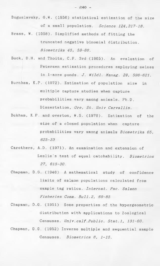
Boguslavsky, G.W. (1956) statistical estimation of the size

of a small population. S c i e n c e 124,317-18.

Brass, W. (1958). Simplified methods of fitting the

truncated negative binomial distribution.

B i o m e t r i k a 45, 59-68.

Buck, D.H. and Thoits, C.F. 3rd (1965). An evaluation of

Petersen estimation procedures employing seines

in 1 -acre ponds. J. Wildl. Manag. 29, 598-621.

Burnham, K.P. (1972). Estimation of population size in

multiple capture studies when capture

probabilities vary among animals. Ph.D.

Dissertation, Ore, St. U n i v C a r v a l l i s .

Bukhara, K.P. and overton, W.S. (1978). Estimation of the

size of a closed population when capture

probabilities vary among animals B i o m e t r i k a 65, 6 2 5 - 3 3

Carothers, A.D. (1971). An examination and extension of

Leslie's test of equal catchability. B i o m e t r i c s 27, 615-30.

Chapman, D.G. (1948) A mathematical study of confidence

limits of salmon populations calculated from

sample tag ratios. Internat. Pac. Salmon F i s h e r i e s Comm. B u l l . 2, 69-85

Chapman, D.G. (1951) Some properties of the hypergeometric

distribution with applications to Zoological

Censuses. U n i v . c a l f . P u b l i c . Stat.l, 131-60.

Chapman, D.G. (1952) Inverse multiple and sequential sample

Censuses. B i o m e t r i c s 8, 1-15.

- 240 -

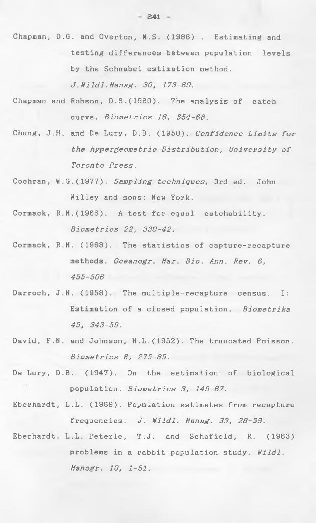
241

Chapman, D.G. and Overton, W.S. (1986) . Estimating and

testing differences between population levels

by the Schnabel estimation method.

J.Wildl.Manag. 30, 173-80.

Chapman and Robson, D.S.(1960). The analysis of catch

curve. B i o m e t r i c s 16, 354-68.

Chung, J.H. and De Lury, D.B. (1950). C o n f i d e n c e L i m i t s for the h y p e r g e o m e t r i e D i s t r i b u t i o n , U n i v e r s i t y of Toronto Press.

Cochran, W.G.(1977). S a m p l i n g techniques, 3rd ed. John

Willey and sons: New York.

Cormack, R.M.(1966). A test for equal catchability.

B i o m e t r i c s 22, 330-42.

Cormack, R.M. (1968). The statistics of capture-recapture

methods. Oceanogr. Mar. Bio. Ann. Rev. 6, 4 5 5 - 5 0 6

Darroch, J.N. (1958). The multiple-recapture census. I:

Estimation of a closed population. B i o m e t r i k a 45, 343-59.

David, F.N. and Johnson, N.L.(1952). The truncated Poisson.

B i o m e t r i c s 8, 275-85.

De Lury, D.B. (1947). On the estimation of biological

population. B i o m e t r i c s 3, 145-67.

Eberhardt, L.L. (1969). Population estimates from recapture

frequencies. J. hfildl. Manag. 33, 28-39.

Eberhardt, L.L. Peterle, T.J. and Schofield, R. (1963)

problems in a rabbit population study. Wildl. Manogr. 10, 1-51.

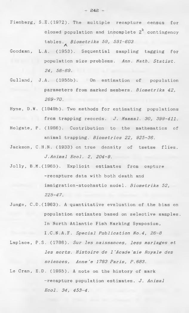
242

Fienberg, S.E.(1972). The multiple recapture census for

closed population and incomplete 2 contingency

tables. B i o m e t r i k a 59, 5 9 1 - 6 0 3 AGoodman, L.A. (1953). Sequential sampling tagging for

population size problems. A n n . Math. Statist. 24, 56-69.

Gulland, J.A. (1955b). On estimation of population

parameters from marked members. B i o m e t r i k a 42, 269-70.

Hyne, D.W. (1949b). Two methods for estimating populations

from trapping records. J. Mammal. 30, 399-411.

Holgate, P. (1966). Contribution to the mathematics of

animal trapping. B i o m e t r i c s 22, 925-36.

Jackson, C.H.N. (1933) on true density of tsetse flies.

J . A n imal Ecol. 2, 204-9.

Jolly, B.M.(1965). Explicit estimates from capture

-recapture data with both death and

immigration-stochastic model. B i o m e t r i k a 52, 225-47.

Junge, C.D.(1963). A quantitative evaluation of the bias on

population estimates based on selective samples.

In North Atlantic Fish Marking Symposium,

I.C.N.A.F. Special P u b l i c a t i o n N o . 4, 2 6 - 8

Laplace, P.S. (1786). Sur les naissances, less m a r i a g e s et les morts. H i s t o i r e de 1 'Acade 'mie R o y a l e d es sciences, A n n e ' e 1783 Paris, P.683.

Le Cran, E.D. (1965). A note on the history of mark

-recapture population estimates. J. Animal Ecol. 34, 453-4.

243

Leslie, P.H.(1952). The estimation of population parameters

from data obtained by means of capture

-recapture method.II: the estimation of total

numbers. B i o m e t r i k a 3 9 , 3 6 3 - 8 8 Manly, B .F .J .(1969). Some properties of a method of

estimating the size of mobile animal

populations. B i o m e t r i k a 56, 407-10.

Marten, G.G.(1970a). A regression method for mark

-recapture estimates with unequal catchability.

E c o l o g y 51,291-5.

Mitra, S.K.(1958). On the limiting power function of the

frequency Chi-Squared test. Ann. Math.

S t a t i s t .29,1221-33

Otis, D.L., Burnham, K.P., White, G.L. and Anerson. D.R.

(1978). Statistical inference for capture data

from closed populations. Wildl. Monogr. No.

62, 135 p . p .

Overton, W.S.(1965). A modification of the schnabel

estimator to account for removal of animals

from the population. J. W i l d l .M a n a g . 29, 392-5. Owen, D .B . ( 1962).H a n d b o o k of s t a t i s t i c a l tables. Addison-

Wesley,Reading, Massachusetts.

Paloheimo,J .E .(1963). Estimation of catchabilities and

population on sizes of lobsters. J. F i s h Res. B d . Cana d a 20,59-88.

Parr, M.J. Gaskell, T.J. and George, B.J. (1968). capture

-recapture methods of estimating animal

numbers. J.Biol. educ 2, 95-117.

Paulik, B.J.(1961). Detection of incomplete reporting of

tags. J. Fish. Res.Bd. C a n a d a 18, 817-29.

244

Pielou, E.C. (1969). An intro d u c t i o n to M a t h e m a t i c a l E c o l o g i c a l , Wiley-Interscience: New York

Pollock, K.H(1974). The assumption of equal catchability

of animals in tag-recapture experiments. PHD.

Dissertation, Cornell Univ. Ithaca, N. Y. Pollock, K.N.(1975a). Building models of capture—recapture

experiments. The statistician, 25,253-60. Pollock, K.H.(1275b). A k-sample. tag-recapture model

allowing for unequal survival and

catchability. B i o m e t r i k a 62, 5 7 7 - 6 3 Rafail, S.Z (1972a) A further contribution to the study of

fish populations by capture-recapture

experiments. M a r i n e B i o l o g y 14, 338-40. Regier, N.A. and Robson, D.S. (1967) Estimating population

number and mortality rates. In S.D. Gerking

(ed. ), The B i o l o g i c a l B a s i s o f F r e s h w a t e r F i s h Production, 31-66. Blackwell Scientific

Publications: Oxford.

Ricker, W.E.(1956). Uses of marking animals in ecological

studies: the marking of fish. E c o l o g y 37, 665-70.

Ricker, W.E. (1958). Handbook of computations for

biological statistics of fish populations.

B u l l . F i s h . B d Canada 119, 1 - 300 Robson, D.S.(1969). Mark-recapture methods of population

estimation Fh N.L. Johnson and H. Smith J.

(Editors) M e w D e v e l o p m e n t in s u r v e y sampling, 120-40. Wiley Interscience, Wiley and Sons : New York.

245

Robson, D.S. and Flick, W.A.(1965) A non parametric

statistical method for calling recruits from a

mark-recapture experiment. B i o m e t r i c s 21,936-47.

Robson, D.S. and Regier, H.A(1964). Sample size in Petersen

mark-recapture experiments Trans. Amer. Fish. Soc. 93, 2 1 5 - 2 6

Samwel, E. (1968). Sequential likelihood estimation of the

size of a population. Ann. Math. Statist.

39, 1 0 5 7 - 6 8

Sanathanan, L.(1972). Estimating the size of a multinomial

population. Ann, Math. Statist. 43, 142-52.

Seber, G .A .F .(1962). The multi-sample recapture census.

B i o m e t r i k a 49, 330-49.

Seber G.A.F (1965). A note on the multiple recapture census

B i o m e t r i k a 52, 249-259.

Seber G.A.F. (1970a). The effects of trap response on

tag-recapture estimates. B i o m e t r i c s 2 6 , 1 3 - 2 2

Seber G .A .F .(1982) . The e s t i mation o f animal abundance. G r i ffin and C o m p a n y London.

Tanaka, R.(1967). New regression formula to estimate the

whole population for recapture addictive small

mammals. Res. Popul. Ecol. 9, 63-94

Welch, H.E.(1960) Two applications of a method of

determining the error of population estimates

of mosquito larvae by the mark and recapture

technique. E c o l o g y 41,228-9.

Young H. Nees. J. and Emlen, J.T.Jr.(1952). Heterogeneity

of trap response in a population of house

246

mice. J. W i l d l .M a n a g .16, 169-80.

Zippin, C.(1958). The removal method of population

estimation J. Wildl. Manag. 22,82-90.