ON THE BETTI NUMBERS OF NODAL SETS OF THE ELLIPTIC EQUATIONS the... · ON THE BETTI NUMBERS OF NODAL SETS OF THE ELLIPTIC EQUATIONS FANGHUA LIN AND DAN LIU Abstract. In this paper

ON THE BETTI NUMBERS OF NODAL SETS OF THE ELLIPTICEQUATIONS

FANGHUA LIN AND DAN LIU

Abstract. In this paper we study the topological properties of the nodal sets, N (u) =

{x : u(x) = 0}, of solutions, u, of second order elliptic equations. We show that the total

Betti number of a nodal set can be controlled by the coefficients and certain numbers of

their derivatives of equations as well as the vanishing order of the corresponding solution.

1. Introduction

The main object of this paper is to study the topological complexity of the nodal sets

of solutions to general elliptic equations. We will in particular study the Betti numbers of

nodal (or general level sets when the zeroth order of equations vanish) sets.

The geometric structure and measure of the nodal sets of real-valued solutions to

the linear elliptic equations have been studied by many authors, see the work of Oleinik-

Petrovskii [24], Cheng ([5]), Donnelly-Fefferman ([7], [8]), Garofalo-Lin ([11]), Han ([13]),

Han-Hardt-Lin ([14]), Hardt-Simon ([15]), Lin([17], [18]) and more recent ones, see for

examples, Cheeger et al ([4]), Colding-Minicozzi ([6]), Hamid-Sogge ([12]), Sogge-Zelditch

([26]). There are also some results for the nodal sets of complex-valued or vector-valued

solutions, see for instance the work of Berger-Rubinstein ([3]), Elliott-Matano-Tang ([9]),

C. Bar ([1]), Helffer-Hoffmann-Hoffmann-Owen ([16]) and X.B. Pan ([23]).

1991 Mathematics Subject Classification. 82D55, 35B25, 35B40, 35Q55.

Key words and phrases. Betti number, nodal set, elliptic PDEs.

1

2 FANGHUA LIN AND DAN LIU

The above works were focused mainly on the following issues: the Hausdorff dimension

and the Hausdorff measure estimates and the local smooth structure of nodal and critical

point sets. For the topological complexity of the nodal sets, say the Betti numbers, there

were only a few results known to authors, Y.Yomdin ([28], [29],[30]). There were, however,

well-known works concerning polynomials done by R. Thom [27] and J. Milnor [21]. In

[21], an upper bound for the sum of the Betti numbers of a real algebraic variety was

proved by using the Morse theory.

Lemma 1.1. ([21]) Let f(x) be a degree N polynomial of x ∈ Rn, then

the total Betti number of f−1(0) ≤ c(n)Nn.

This result shows that the total Betti number can be bounded by a constant depending

on the degree of the polynomial and the number of unknowns. From earlier analysis for

nodal and critical point sets of solutions of elliptic equations, one tends to believe that

the analogy may be also valid for bounds on Betti numbers. Indeed, solutions of elliptic

equations possess properties similar to that of analytic functions. Naturally, the first step

one needs to do would be to control the so-called ”generalized degrees” of solutions. This

generalized degree has a natural substitute, the Almgren’s frequency, which has already

been applied in the study of the quantitative unique continuation property of solutions,

see for example, [11]. The next important step would be to get a more quantified version of

Morse Theory that J.Milnor had used in the above lemma. Very much like a quantitative

version of Stability Lemma in Han-Hardt-Lin [14] which played a critical role in obtaining

the geometric measure estimates for critical sets of solutions, the compactness of solutions

of second order elliptic equations with an uniformly bounded vanishing order would be

crucial. In order for a suitable perturbation argument to work which is necessary for

BETTI NUMBER 3

understanding solutions of elliptic equations which are in general non-analytic, one also

requires coefficients of equations to be uniformly elliptic and to be of certain fixed number

of orders of smoothness.

Let us first introduce some notations. Throughout this paper, we consider the general

elliptic equation,

n∑i,j=1

aij(x)Diju(x) +n∑i=1

bi(x)Diu(x) + c(x)u(x) = 0 in B1(0) ⊂ Rn, (1.1)

where the coefficients satisfy the following assumptions:

λ|ξ|2 ≤3∑

i,j=1

aij(x)ξiξj ≤ Λ|ξ|2, ∀ξ ∈ R3, x ∈ B1(0), (1.2)

and for a suitably large M

n∑i,j=1

‖aij‖CM,α(B1(0)) +n∑i=1

‖bi‖CM,α(B1(0)) + ‖c‖CM,α(B1(0)) ≤ K. (1.3)

where λ,Λ and K are positive constants.

The following theorem is the main result of the paper:

Theorem 1.2. Let u be the solution of problem (1.1), and the coefficients aij, bi and

c satisfy the conditions (1.2) and (1.3). Here M may chosen to be 2(2N0)n. Then for

B 12(0),

the total Betti numbers of N (u) ∩B 12(0) ≤ C(n,K, λ,Λ, N0).

where the constant N0 is the upper bound of the vanishing order of u at any point of B 12(0).

In Section 3 below, we will give the precise definition of the vanishing order and the

existence of an uniformly upper bound for N0.


This paper is organized as follows. In Section 2, we prove some stability results,

which play a crucial role in the proof of Theorem 1.2. In Section 3, after recalling the

definition of the vanishing order of u, we give a natural definition of the Betti numbers

of N (u) ∩ B 12(0). As the nodal sets may not be in general a smooth hypersurface, the

notation of its Betti numbers have to be defined properly. We end with this section the

proof of the main theorem.

Achownkegements : Much of the work was carried out while the second author was

visiting the Courant Institute during the academic year 2010 − 2011. She would like

to thank the Courant Institute of Mathematical Sciences of the New York University

for sponsoring this visit and for provide a great academic atmosphere and facilities. The

research of the first author is partial supported by the NSF grant, DMS-1065964 and DMS-

1159313. The research of the second author is supported by the national Postdoctoral

Science Foundation of China and the Shanghai Postdoctoral Science Foundation under

the Grant numbers 2013M530186 and 13R2142500.

2. stability results

In this section we prove some stability results, which will be used in the proof of

Theorem 1.2. First, we prove a general statement 2.1 which is somewhat standard in the

study of stability of singularities in the algebra geometry. Given some smooth map g,

the stability result holds for any smooth map sufficiently close to g with the closeness

measured by several constants all depending on g. If we take the map g as a polynomial

map in a suitable family that comes naturally from the Taylor expansions of solutions

to a wide class of elliptic equations with an uniform bound on the vanishing orders, we

BETTI NUMBER 5

get a stronger stability statement in Lemma 2.3. Roughly speaking, given N0, for all (L-

harmonic) polynomial maps g with degrees less than 2N0 and with the Almgren frequencies

of g bounded by N0, then the constants can be chosen to depend only on N0 and the

dimension such that the conclusion of the stability lemma holds.

We start with the following lemma:

Lemma 2.1. Let G(x) = (g1(x), · · · , gn(x)) be a smooth map defined from B1(0) ⊂ Rn to

Rn. Assume that the extended map G(x) from the unit ball in Cn to Cn is holomorphic.

If

H0{G−1(0) ∩B1(0)} = m <∞,

then there exist positive constants δ∗, M∗, r∗ and C∗ all depending on the function G(x),

such that for any F (x) = (f1(x), · · · , fn(x)) ∈ CM∗(B1(0)) with

‖F −G‖CM∗ (B1(0)) < δ∗,

we have

H0{F−1(0) ∩Br∗(0)

}≤ C∗

with multiplicity.

Proof. The proof is given in [14, Theorem 4.1]. For the sake of the completeness, we sketch

it here. Assume that the nodal set of G = (g1, g2, · · · , gn) contains m points, letting

N (G) = H0{G−1(0) ∩B1(0)

}= {0, x1, · · · , xm−1}.

Step 1. For 0 ∈ N (G), one can show that there is an integer N0j and a holomorphic

function a0ij(x) such that,

xN0j

j =n∑i=1

a0ij(x)gi(x), for each j = 1, 2, · · · , n,


where x ∈ Rn.

Letting Λ0 = nmax{N01 , N

02 , · · · , N0

n}, then any monomial in x1, · · · , xn of degree

≥ Λ0 belongs to the ideal (G) near 0. Therefore, we can choose an integer µ0 such that

dimRPµ0/(G) ≤ µ0,

where the set Pµ0(Rn) denotes the collection of all polymomials in R of degree µ0.

Following the arguments in the proof of Theorem 4.1 ([14]), we obtain that there exist

neighborhoods U0, V0 and Q0 of the origin with V0 ⊂ U0 and G(V0) ⊂ Q0 such that for

any a ∈ C2µ0(U0) there exist α01, α

02, · · · , α0

n ∈ C1(Q0) such that

a(x) =µ0∑i=1

ei(x)α0i (g(x)), for x ∈ V0. (2.1)

Moreover, there exists a δ0 > 0, such that for any F ∈ C2µ0(U0) with ‖F−G‖C2µ0 (U0) < δ0,

the identity (2.1) still holds with G replaced by F .

As in ([14]), there exists r0 > 0, such that F has µ0 zeros at most in Br0(0).

Step 2. For each xk ∈ N (G), we repeat the step 1 to get corresponding µk, Uk, Vk, Qk,

δk and rk, such that for F with ‖F −G‖C2µk (Uk)< δk, F has µk zeros at most in Brk(xk).

Therefore, by taking

δ∗ = min{δ0, · · · , δm−1}, M∗ = 2m−1∑k=0

µk, C∗ =m−1∑k=0

µk,

and choosing r∗ such that

Br∗(0) ⊂m−1⋃k=0

Brk(xk) ⊂m−1⋃k=0

Vk,

we have,

H0{F−1(0) ∩Br∗(0)

}≤ C∗.

BETTI NUMBER 7

for F (x) ∈ CM∗(B1(0)) with ‖F − G‖CM∗ (B1(0)) < δ∗. To end our proof, we remark that

the constants M∗, δ∗, r∗ and C∗ all depend on G(x). �

Remark 1. In general, the constant M∗ may be very large, which means the function

F (x) must have sufficiently higher orders of derivatives. It is the reason why we need the

assumption (1.3) to make sure solutions of such equations would be also sufficiently smooth

for the conclusion of Theorem 1.2 to be valid. On the other hand, if G is a polynomial of

degree at most N , then from the above proof of ([14]), M∗ may be chosen to be not bigger

than 2Nn.

Remark 2. Let us introduce the set

GN0 = {g(x) : B1(0)→ R1, a polynomial in B1(0) ⊂ Rn, with degree ≤ 2N0, ‖g‖L2 = 1,

�B1(0)

|∇g|2dx ≤ N0}.

Then GN0 is a compact set in the polynomial space of CM∗, see for example, [14].

For given numbers ε and θ in [0, 1] we also define the set

FN0 = {f : f = g2 + ε2|x|2 − θ2, g ∈ GN0}.

Then FN0 is also compact.

Corollary 2.2. For a given f0 ∈ FN0, there exist positive constants M0, r0, δ0 and

C0, such that if f ∈ CM0+1(B1(0)) with ‖f − f0‖CM0+1 < δ0, and the hypersurfaces

{x : f(x) = 0} and {x : f0(x) = 0} are both regular, then

H0{F−1(0) ∩Br0(0)

}≤ C0,

where F is a vector feild defined by F (x) = ( ∂f∂x1, · · · , ∂f

∂xn−1, f), for a suitable choice of

rectangular coordinate system (x1, x2, · · · , xn) of Rn.


Proof. First, Let us use the following notations for the two hypersurfaces:

W1 = {x ∈ B1(0) : f0(x) = 0} , W2 = {x ∈ B1(0) : f(x) = 0} .

We use ~n1 and ~n2 to denote the Gaussian maps of W1 and W2. Sard’s theorem ensures

that the sets

{~n1 : ∇~n1 = 0} and {~n2 : ∇~n2 = 0}

both have measure zero in Sn−1.

Up to some coordinate rotation, we may choose directions (0, · · · , 0, 1) ∈ Rn, such

that ~n1(q) = (0, · · · , 0, 1), and (0, · · · , 0, 1) are neither the critical values of ~n1 nor the

critical values of ~n2.

Therefore, the height function (x1, · · · , xn) → xn of the hypersurfaces W1 and W2

has no degenerate critical points. And the critical points of the height function on W1 and

W2 can be characterized as the solutions of the equations

F0(x) = (∂f0

∂x1, · · · , ∂f0

∂xn−1, f0) = 0, F (x) = 0.

Since f0 is a polynomail of degree ≤ 2N0, we can apply the result of [21] to obtain

that

H0{F−1

0 (0) ∩B1(0)}

= m0 <∞.

For any f ∈ CM0+1(B1(0)), we have ‖F − F0‖CM0 (B1(0)) < δ0. Applying Lemma 2.1

to the maps F and F0, there exist positive constants r0 and C0 depending on f0, such that

H0{F−1(0) ∩Br0(0)

}≤ C0.

�

The next Stability Lemma is the key to our proof of the main theorem.

BETTI NUMBER 9

Lemma 2.3. There exist positive constants δ0, M0, r0 and C0 only depending on N0,

such that if f ∈ CM0+1(B1(0)), and if the hypersurface {x : f(x) = 0} is regular with

‖f − g‖CM0+1(B1(0)) < δ0 and g ∈ FN0, satisfying that {x : g = 0} is also a regular

hypersurface, then we have

H0{F−1(0) ∩Br0(0)

}≤ C0,

where the map F (x) = ( ∂f∂x1, · · · , ∂f

∂xn−1, f), for a suitable choice of rectangular coordinate

system (x1, x2, · · · , xn) of Rn.

Proof. From Corollary 2.2, we can see that for each g ∈ FN0 , there exist positive constants

δg, Mg, rg and Cg, such that if ‖g − f‖CMg+1(B1(0)) < δg, then

H0{F−1(0) ∩Brg(0)

}≤ Cg.

Let us remark that the constants Mg and Cg for any g can be chosen uniformly

depending only on N0, say 2(2N0)n.

Therefore, {O(g, δg2 ) : g ∈ FN0}, form an open cover of FN0 . By the compactness of

FN0 , there exists a finite cover, denoted by

FN0 ⊂k⋃j=1

O(gj ,δ02

).

Let us denote the representatives by RF = {g1, · · · , gk}, and we take

δ0 =12

min{δ1, · · · , δk}, r0 = min{r1, · · · , rk}.

We claim that the constants δ0 and r0 only depend on N0. In other words, for any g ∈ FN0 ,

the stability results holds for δ0 and r0.


In fact, for any given g ∈ FN0 , by the above covering of FN0 , there exists some

gs ∈ RF , such that ‖gs−g‖CM0+1 < δs2 . If f ∈ CM0+1(B1(0)) with ‖f−g‖CM0+1(B1(0)) < δ0,

then

‖f − gs‖CM0+1(B1(0)) < δ0 +δs2≤ δs

2+δs2

= δs.

Applying Corollary 2.2 to gs, we get

H0{F−1(0) ∩Br0(0)

}⊂ H0

{F−1(0) ∩Brs(0)

}≤ C0.

Hence the stability result works uniformly for the fixed constants δ0 and r0, which only

depend on N0.

Therefore, if f ∈ CM0+1(B1(0)) with ‖f − g‖CM0+1(B1(0)) < δ0 for some g ∈ FN0 , we

may conclude that

H0

{(∂f

∂x1, · · · , ∂f

∂xn−1, f)−1(0) ∩Br0

}≤ C0,

which completes the proof. �

3. Estimates on the total Betti numbers

We can now give an upper estimate of the total Betti numbers of a nodal set. To

begin with, let us recall the definition of vanishing order of u.

Assume that u ∈ W 1,2(B1(0)) is a solution of (1.1) in B1(0) ⊂ Rn. To define the

vanishing order of the weak solution u, we only need the following weaker assumptions on

the coefficients than (1.2) and (1.3):

3∑i,j=1

aij(x)ξiξj ≤ λ|ξ|2, ∀ξ ∈ R3, x ∈ B1(0),

n∑i,j=1

|aij |+n∑i=1

|bi|+ |c| ≤ κ, ∀ x ∈ B1(0), (3.1)

BETTI NUMBER 11

n∑i,j=1

|aij(x)− aij(y)| ≤ L|x− y|, ∀ x, y ∈ B1(0),

for some positive constants λ, κ and L.

In [11], the authors define,

H(p, r) =�∂Br(p)

µu2dx,

D(p, r) =�Br(p)

aij(x)uxiuxjdx,

where the positive function µ is constructed in [11].

Letting

N(p, r) =rD(p, r)H(p, r)

,

a monotonicity property for N(p, r) with respect to r is proved in [11]: there exist positive

constants r0 = r0(n, λ, κ, L) and θ = θ(n, λ, κ, L) such that the function N(p, r)exp(θr) is

monotone nondecreasing in (0, r0).

Therefore, one can define at each point p ∈ B 12(0) the quantity,

Ou(p) := limr→0

N(p, r).

We shall call it the vanishing order of u at point p. The following lemma says that the

vanishing order of u in B 12(0) is uniformly bounded. For details see [17]. In our paper, we

denote the uniformly upper bound by the constant N0.

Lemma 3.1 ([17]). Set

N =

�B1(0) |Du|

2dx�∂B1(0) u

2dx.

Then the vanishing order of u at any point of B1/2(0) is never exceeded by C(n, λ, κ, L)N .


The following lemma comes from [13] and [14]. It yields a decomposition result and

Schauder estimates of the error term.

Lemma 3.2 ([13], [14]). Suppose that u is the solution to the equation (1.1). Under the

assumption (3.1), for any y ∈ B1/2(0), the solution u has the following decomposition:

u(x) = Pd(x− y) + φ(x), x ∈ B1/4(y), (3.2)

where the nonzero polynomial Pd(x−y) is homogeneous of degree d = d(y) ≤ N0 satisfying

n∑i,j=1

aij(y)DijPd = 0, (3.3)

and

|Pd(x− y)| ≤ C|x− y|d, x ∈ B1/4(y). (3.4)

Moreover φ satisfies the following estimate: for some α ∈ (0, 1),

|φ(x)| ≤ C|x− y|d+α, x ∈ B1/4(y). (3.5)

The constant C depends on n,N0, λ, κ, L.

Furthermore, if we assume that the assumptions (1.2) and (1.3) hold, by using the

interior Schauder estimates one can get,

|Diφ(x)| ≤ C|x− y|d−i+α, for i = 1, · · · , d,

|Diφ(x)| ≤ C, for i = d+ 1, · · · , M + 1,

(3.6)

for all x ∈ B1/8(y). The positive constant C depends on n,N0, λ,Λ,K.

Next, let us use the definition of the total Betti number of N (u) ∩B1/2(0) in [21]:

Definition 3.1. The total Betti numbers of N (u) ∩B1/2(0) is defined to be

BETTI NUMBER 13

the lim sup(ε,θ)→(0+,0+) of the total Betti numbers of N(ε,θ)(u) ∩B1/2(0),

where N(ε,θ)(u) ∩B1/2(0) = {x ∈ Rn : u2 + ε2|x|2 = θ2}.

Before we prove Theorem 1.2, let us also recall the weak Morse inequalities (see [22]).

Lemma 3.3 ([22]). (Weak Morse Inequalities) Let bk be the k-th Betti number of a

compact manifold M and ck denote the set of the critical points of index k of a Morse

function on M , then

bk ≤ #ck, for all k ∈ [0, dimM ],

anddimM∑k=0

(−1)k#ck =dimM∑k=0

(−1)kbk = χ(M).

By the above lemma, it is therefore sufficient for us to do the following two things.

One is to construct suitable Morse functions. The other is to get a suitable estimate of

the numbers of critical points of such Morse functions.

The following lemma comes from [21]. It gives an estimate on the number of zeros of

polynomial equations.

Lemma 3.4 ([21]). Let V0 ⊂ Rm be a zero-dimensional variety defined by polynomial

equations f1 = 0, · · · , fm = 0. Suppose that the gradient vectors df1, · · · , dfm are linearly

independent at each point of V0. Then the number of points in V0 is at most equal to the

product (degf1)(degf2) · · · (degfm).

Now we can proceed with the proof of Theorem 1.2: Taking any fixed point y0 ∈

N (u) ∩B1/2(0), there exists a nonzero homogeneous polynomial Pd of degree 0 ≤ d ≤ N0


such that

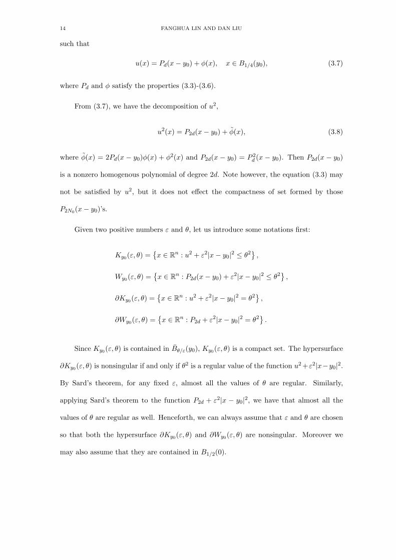
u(x) = Pd(x− y0) + φ(x), x ∈ B1/4(y0), (3.7)

where Pd and φ satisfy the properties (3.3)-(3.6).

From (3.7), we have the decomposition of u2,

u2(x) = P2d(x− y0) + φ(x), (3.8)

where φ(x) = 2Pd(x − y0)φ(x) + φ2(x) and P2d(x − y0) = P 2d (x − y0). Then P2d(x − y0)

is a nonzero homogenous polynomial of degree 2d. Note however, the equation (3.3) may

not be satisfied by u2, but it does not effect the compactness of set formed by those

P2N0(x− y0)’s.

Given two positive numbers ε and θ, let us introduce some notations first:

Ky0(ε, θ) ={x ∈ Rn : u2 + ε2|x− y0|2 ≤ θ2

},

Wy0(ε, θ) ={x ∈ Rn : P2d(x− y0) + ε2|x− y0|2 ≤ θ2

},

∂Ky0(ε, θ) ={x ∈ Rn : u2 + ε2|x− y0|2 = θ2

},

∂Wy0(ε, θ) ={x ∈ Rn : P2d + ε2|x− y0|2 = θ2

}.

Since Ky0(ε, θ) is contained in Bθ/ε(y0), Ky0(ε, θ) is a compact set. The hypersurface

∂Ky0(ε, θ) is nonsingular if and only if θ2 is a regular value of the function u2 +ε2|x−y0|2.

By Sard’s theorem, for any fixed ε, almost all the values of θ are regular. Similarly,

applying Sard’s theorem to the function P2d + ε2|x − y0|2, we have that almost all the

values of θ are regular as well. Henceforth, we can always assume that ε and θ are chosen

so that both the hypersurface ∂Ky0(ε, θ) and ∂Wy0(ε, θ) are nonsingular. Moreover we

may also assume that they are contained in B1/2(0).

BETTI NUMBER 15

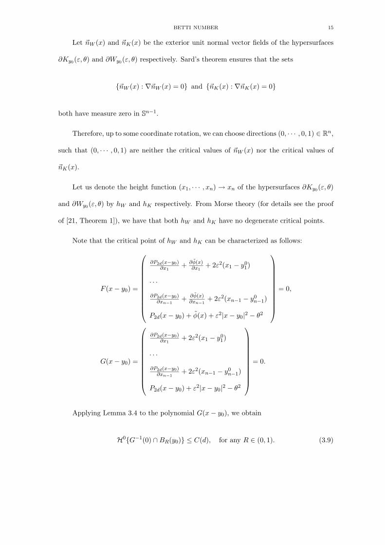
Let ~nW (x) and ~nK(x) be the exterior unit normal vector fields of the hypersurfaces

∂Ky0(ε, θ) and ∂Wy0(ε, θ) respectively. Sard’s theorem ensures that the sets

{~nW (x) : ∇~nW (x) = 0} and {~nK(x) : ∇~nK(x) = 0}

both have measure zero in Sn−1.

Therefore, up to some coordinate rotation, we can choose directions (0, · · · , 0, 1) ∈ Rn,

such that (0, · · · , 0, 1) are neither the critical values of ~nW (x) nor the critical values of

~nK(x).

Let us denote the height function (x1, · · · , xn) → xn of the hypersurfaces ∂Ky0(ε, θ)

and ∂Wy0(ε, θ) by hW and hK respectively. From Morse theory (for details see the proof

of [21, Theorem 1]), we have that both hW and hK have no degenerate critical points.

Note that the critical point of hW and hK can be characterized as follows:

F (x− y0) =

∂P2d(x−y0)∂x1

+ ∂φ(x)∂x1

+ 2ε2(x1 − y01)

· · ·

∂P2d(x−y0)∂xn−1

+ ∂φ(x)∂xn−1

+ 2ε2(xn−1 − y0n−1)

P2d(x− y0) + φ(x) + ε2|x− y0|2 − θ2

= 0,

G(x− y0) =

∂P2d(x−y0)∂x1

+ 2ε2(x1 − y01)

· · ·

∂P2d(x−y0)∂xn−1

+ 2ε2(xn−1 − y0n−1)

P2d(x− y0) + ε2|x− y0|2 − θ2

= 0.

Applying Lemma 3.4 to the polynomial G(x− y0), we obtain

H0{G−1(0) ∩BR(y0)} ≤ C(d), for any R ∈ (0, 1). (3.9)


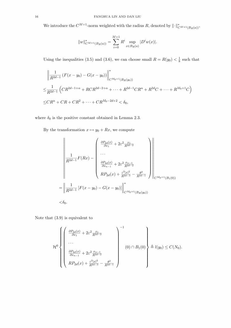
We introduce the CM+1-norm weighted with the radius R, denoted by ‖·‖∗CM+1(BR(a))

,

‖w‖∗CM+1(BR(a)) =M+1∑i=0

Ri supx∈BR(a)

|Diw(x)|.

Using the inequalities (3.5) and (3.6), we can choose small R = R(y0) < 18 such that

∥∥∥∥ 1R2d−1

(F (x− y0)−G(x− y0))∥∥∥∥∗CM0+1(BR(y0))

≤ 1R2d−1

(CR2d−1+α +RCR2d−2+α + · · ·+R2d−1CRα +R2dC + · · ·+RM0+1C

)≤CRα + CR+ CR2 + · · ·+ CRM0−2d+2 < δ0,

where δ0 is the positive constant obtained in Lemma 2.3.

By the transformation x 7→ y0 +Rx, we compute∥∥∥∥∥∥∥∥∥∥∥∥∥∥∥∥1

R2d−1F (Rx)−

∂P2d(x)∂x1

+ 2ε2 x1

R2d−2

· · ·

∂P2d(x)∂xn−1

+ 2ε2 xn−1

R2d−2

RP2d(x) + ε2|x|2R2d−3 − θ2

R2d−1

∥∥∥∥∥∥∥∥∥∥∥∥∥∥∥∥CM0+1(B1(0))

=∥∥∥∥ 1R2d−1

[F (x− y0)−G(x− y0)]∥∥∥∥∗CM0+1(BR(y0))

<δ0.

Note that (3.9) is equivalent to

H0

∂P2d(x)∂x1

+ 2ε2 x1

R2d−2

· · ·

∂P2d(x)∂xn−1

+ 2ε2 xn−1

R2d−2

RP2d(x) + ε2|x|2R2d−3 − θ2

R2d−1

−1

(0) ∩B1(0)

, l(y0) ≤ C(N0).

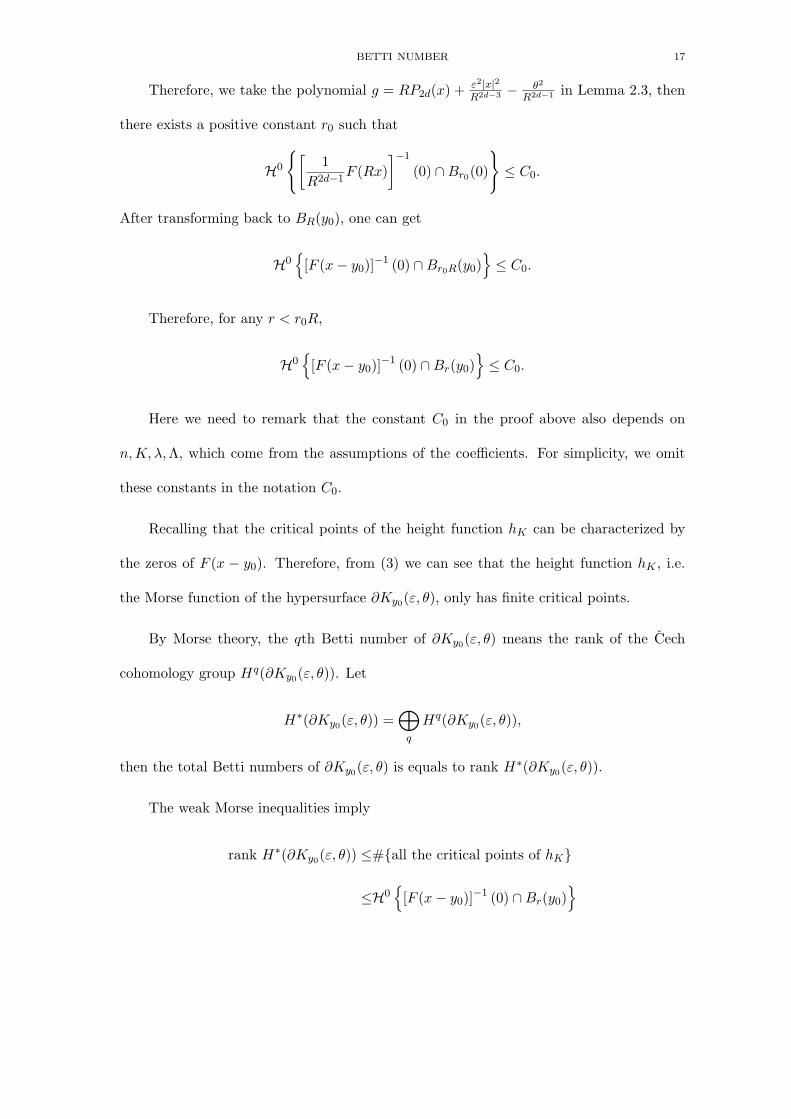
BETTI NUMBER 17

Therefore, we take the polynomial g = RP2d(x) + ε2|x|2R2d−3 − θ2

R2d−1 in Lemma 2.3, then

there exists a positive constant r0 such that

H0

{[1

R2d−1F (Rx)

]−1

(0) ∩Br0(0)

}≤ C0.

After transforming back to BR(y0), one can get

H0{

[F (x− y0)]−1 (0) ∩Br0R(y0)}≤ C0.

Therefore, for any r < r0R,

H0{

[F (x− y0)]−1 (0) ∩Br(y0)}≤ C0.

Here we need to remark that the constant C0 in the proof above also depends on

n,K, λ,Λ, which come from the assumptions of the coefficients. For simplicity, we omit

these constants in the notation C0.

Recalling that the critical points of the height function hK can be characterized by

the zeros of F (x − y0). Therefore, from (3) we can see that the height function hK , i.e.

the Morse function of the hypersurface ∂Ky0(ε, θ), only has finite critical points.

By Morse theory, the qth Betti number of ∂Ky0(ε, θ) means the rank of the Cech

cohomology group Hq(∂Ky0(ε, θ)). Let

H∗(∂Ky0(ε, θ)) =⊕q

Hq(∂Ky0(ε, θ)),

then the total Betti numbers of ∂Ky0(ε, θ) is equals to rank H∗(∂Ky0(ε, θ)).

The weak Morse inequalities imply

rank H∗(∂Ky0(ε, θ)) ≤#{all the critical points of hK}

≤H0{

[F (x− y0)]−1 (0) ∩Br(y0)}


≤C0.

On the other hand, the Alexander duality theorem gives

rank H∗(Ky0(ε, θ)) =12

rank H∗(∂Ky0(ε, θ)).

Hence,

rank H∗(Ky0(ε, θ)) ≤ C0.

Now we can choose suitable sequences {εi} and {θi}, such that {εi} decreases mono-

tonely with the limit zero and {θi/εi} decreases monotonely with limit r(y0). Meanwhile

each ∂Ky0(εi, θi) is a nonsingular hypersurface.

It is easy to see that

K(ε1, θ1) ⊃ K(ε2, θ2) ⊃ · · · ⊃ K(εn, θn) ⊃ · · · ,

and

N (u) ∩Br(y0)(y0) =+∞⋂i=1

K(εi, θi).

Therefore,

rank H∗(N (u) ∩Br(y0)(y0)) ≤ lim sup rank H∗(Ky0(εi, θi)) ≤ C0.

It is obvious that the collection of{Br(y)(y) : y ∈ N (u) ∩B1/2(0)

}covers N (u) ∩

B1/2(0). By the compactness of N (u) ∩ B1/2(0), there exist finite balls {Brj (yj) : j =

1, · · · , ν} such that

N (u) ∩B1/2(0) ⊂ν⋃j=1

Brj (yj),

and for each j,

rank H∗(N (u) ∩Brj (yj)) ≤ C0.

BETTI NUMBER 19

Therefore,

the total Betti numbers of N (u) ∩B1/2(0) ≤ C(N0,K, λ,Λ, n),

which completes the proof of the main theorem. 2

References

[1] C. Bar, Zero sets of solutions to semilinear elliptic systems of first order. Invent. Math. 138 (1999), no.

1, 183202.

[2] V. I. Bakhtin, , The Weierstrass-Malgrange preparation theorem in the finitely smooth case, Func. Anal.

Appl. 24 (1990), 86-96.

[3] J. Berger and J. Rubinstein, On the zero set of the wave function in superconductivity, Comm. Math.

Phys., 202 (1999), 621-628.

[4] J. Cheeger, A. Naber and D. Valtorta, Critical sets of elliptic equations, arXiv:1207.4236.

[5] S. Y. Cheng, Eigenfunctions and nodal sets, Comment. Math. Helv., 51 (1976), no.1, 43-55.

[6] T. H. Colding, W. P., II. Minicozzi, Lower bounds for nodal sets of eigenfunctions. Comm. Math. Phys.

306 (2011), no. 3, 777784.

[7] H. Donnelly and C. Fefferman, Nodal sets of eigenfunctions on Riemannian manifolds, Invent. Math.,

93 (1988), 161-183.

[8] H. Donnelly and C. Fefferman, Nodal sets for eigenfunctions of the Laplacian on surfaces, J. Amer.

Math. Soc., 3 (1990), no. 2, 333-353.

[9] C. M. Elliott , H. Matano and Qi Tang, Zeros of a complex Ginzburg-Landau order parameter with

applications to superconductivity, European J. Appl. Math., 5 (1994), 431–448.

[10] H. Federer, Geometric measure theory, Springer-Verlag, Berlin, 1969.

[11] N. Garofalo and F.-H. Lin, Monotonicity properties of variational integrals, Ap weights and unique

continuation, Indiana Univ. Math. J., 35 (1986), 245-268.

[12] H. Hamid, C. D. Christorpher, A natural lower bound for the size of nodal sets. Anal. PDE 5 (2012),

no. 5, 11331137.

[13] Q. Han, Singular sets of solutions to elliptic equations, Indiana Univ. Math. J., 43 (1994), 983-1002.


[14] Q. Han, R. Hardt and F.-H. Lin, Geometric measure of singular sets of elliptic equations, Comm.

Pure Appl. Math., 51 (1998), 1425-1443.

[15] R. Hardt and L. Simon, Nodal sets for solutions of elliptic equations, J. Diff. Geom., 30 (2) (1989),

505-522.

[16] B. Helffer, M. Hoffmann-Ostenhof, T. Hoffmann-Ostenhof, and M. Owen, Nodal sets for groundstates

of Schrodinger operators with zero magnetic field in nonsimple connected domains, Comm. Math. Phys.,

202 (1999), 629-649.

[17] F.-H. Lin, Nodal sets of solutions of elliptic and parabolic equations, Comm. Pure Appl. Math., 45

(1991), 287-308.

[18] F.-H. Lin, Complexity of solutions of partial differential equations, Handbook of geometric analysis.

No.1, 229-258, Adv. Lect. Math., 7, Int. Press, Someerville, MA, (2008).

[19] F.-H. Lin and X.P. Yang, Geometric measure theory: an introduction, Advanced Mathematics (Bei-

jing/Boston), 1. Science Press, Beijing; International Press, Boston, MA, 2002.

[20] D. Liu, Hausdorff measure of critical sets of solutions to magnetic Schrodinger equations, Cal. Var.

PDEs., 41(1-2), 2011, 179-202.

[21] J. Milnor, On the Betti numbers of real varieties, Proc. Amer. Math. Soc., 15 (1964) 275-280.

[22] J. Milnor, Morse theory, Princeton University Press, Princeton, N.J., 1963.

[23] X. B. Pan, Nodal sets of solutions of equations involving magnetic Schrodinger operator in 3-

dimensions, J. Math. Phys., 48 (2007).

[24] I. G. Petrovski, O. A. Olenik, On the topology of real algebraic surfaces. Amer. Math. Soc. Translation

1952, (1952). no. 70, 20 pp. 14.0X.

[25] A. Sard, The measure of the critical values of differentiable maps, Bull. Amer. Math. Soc. 48, (1942),

883-897.

[26] C. D. Sogge, S. Zelditch, Lower bounds on the Hausdorff measure of nodal sets. Math. Res. Lett. 18

(2011), no. 1, 2537.

[27] R. Thom, Sur l’homologie des varits algbriques relles. (French) 1965 Differential and Combinatorial

Topology (A Symposium in Honor of Marston Morse) pp. 255265 Princeton Univ. Press, Princeton, N.J.

BETTI NUMBER 21

[28] Y. Yomdin, The geometry of critical and near-critical values of differentiable mappings, Math. Ann.,

264, (1983), 495-515.

[29] Y. Yomdin, The set of zeroes of an ”almost polynomial” function, Proc. Amer. Math. Soc., 90, (1984),

538-542.

[30] Y. Yomdin, Global bounds for the Betti numbers of regular fibers of differentiable mappings, Topology,

24, (1985), 145152.

(Fanghua Lin) Courant Institute of Mathematical Sciences, 251 Mercer Street, New

York, NY10012. NYU-ECNU Institute of Mathematical Sciences at NYU Shanghai, 3663,

North Zhongshan Rd., Shanghai, PRC 200062

(Dan Liu) Center for partial differential equations, East China Normal University,

Shanghai 200062, P.R. China

E-mail address, Fanghua Lin: [email protected]

E-mail address, Dan Liu: [email protected]

Documents

ON THE BETTI NUMBERS OF NODAL SETS OF THE ELLIPTIC EQUATIONS the... · ON THE BETTI NUMBERS OF NODAL SETS OF THE ELLIPTIC EQUATIONS FANGHUA LIN AND DAN LIU Abstract. In this paper