On the Behrens-Fisher problem: A globally convergent

The Annals of Statistics2008, Vol. 36, No. 5, 2377–2408DOI: 10.1214/07-AOS528© Institute of Mathematical Statistics, 2008

ON THE BEHRENS–FISHER PROBLEM: A GLOBALLYCONVERGENT ALGORITHM AND A FINITE-SAMPLE STUDY OF

THE WALD, LR AND LM TESTS

BY ALEXANDRE BELLONI1 AND GUSTAVO DIDIER

Duke University and Tulane University

In this paper we provide a provably convergent algorithm for the multi-variate Gaussian Maximum Likelihood version of the Behrens–Fisher Prob-lem. Our work builds upon a formulation of the log-likelihood functionproposed by Buot and Richards [5]. Instead of focusing on the first order op-timality conditions, the algorithm aims directly for the maximization of thelog-likelihood function itself to achieve a global solution. Convergence proofand complexity estimates are provided for the algorithm. Computational ex-periments illustrate the applicability of such methods to high-dimensionaldata. We also discuss how to extend the proposed methodology to a broaderclass of problems.

We establish a systematic algebraic relation between the Wald, LikelihoodRatio and Lagrangian Multiplier Test (W ≥ LR ≥ LM) in the context of theBehrens–Fisher Problem. Moreover, we use our algorithm to computationallyinvestigate the finite-sample size and power of the Wald, Likelihood Ratio andLagrange Multiplier Tests, which previously were only available through as-ymptotic results. The methods developed here are applicable to much higherdimensional settings than the ones available in the literature. This allows usto better capture the role of high dimensionality on the actual size and powerof the tests for finite samples.

1. Introduction. The so-called Behrens–Fisher Problem may be straightfor-wardly stated as follows.

Given two independent random samples X1, . . . ,XN1 and Y1, . . . , YN2 , test whethertheir respective population means μ1 and μ2 coincide in the case where their covari-ances �1 and �2 are unknown.

Despite the deceiving simplicity of its form, this problem has motivated a wealthof literature that began with the original works of Behrens [1] and Fisher [9, 10],and includes Welch [34, 35], Scheffé [26, 27], Yao [37], Robbins, Simons andStarr [23], Subrahmanian and Subrahmanian [33] and Cox [8], to name a few. Fora review of the solutions for the BFP, see, for instance, Stuart and Ord [32] and Kim

Received April 2007; revised June 2007.1Supported in part by the IBM Herman Goldstein Fellowship.AMS 2000 subject classification. 62H15.Key words and phrases. Behrens–Fisher Problem, high-dimensional data, hypothesis testing, al-

gorithm, Wald Test, Likelihood Ratio Test, Lagrange Multiplier Test, size, power.

2377

http://www.imstat.org/aos/

http://dx.doi.org/10.1214/07-AOS528

http://www.imstat.org

2378 A. BELLONI AND G. DIDIER

and Cohen [15]. The proposed solutions involve a myriad of different approaches,ranging from fiducial inference to Bayesian techniques.

In this paper we are interested in the classical multivariate version of theBehrens–Fisher Problem under Normality. In other words, Xi , Yj above shouldbe interpreted as d-dimensional Gaussian random vectors with (vector) means μ1and μ2, and �1, �2 as their respective d ×d covariance matrices, where the samplesizes are greater than d . The sample covariance matrices are then positive definite(and thus invertible) with probability one if the true covariance matrices �1 and�2 are positive definite. Several applied problems can be formulated as Behrens–Fisher Problems (in particular, for high dimension) in diverse areas such as SpeechRecognition (e.g., Chien [6]), Quality Control (e.g., Murphy [21]), DevelopmentEconomics (e.g., Schramm, Renn and Biles [28]) and others.

In this context, the Likelihood Ratio Test is a natural choice in face of the well-known asymptotic behavior of the test statistic. It turns out, though, that the max-imization of the log-likelihood function without restrictive assumptions on thecovariances (e.g., �1 = �2) is a nontrivial matter. In general, explicit solutionsto the maximization procedure do not exist, and due to nonconcavities in the ob-jective function, the solution to the system of first order likelihood equations canlead to local optima, as shown in Buot and Richards [5]. Numerical algorithms areavailable in the literature (see, e.g., Mardia, Kent and Bibby [20] and Buot andRichards [5]), but their convergence properties are unknown.

The purpose of this paper is two-fold. First, to propose a provably convergent al-gorithm, called Cutting Lines Algorithm (CLA), for the Gaussian Maximum Like-lihood Behrens–Fisher Problem (BFP, for short). Second, to use the algorithm toinvestigate the finite sample properties—size and power—of the Likelihood Ra-tio Test and of the asymptotically equivalent Wald and Lagrange Multiplier Testsin the context of the BFP. Such properties are generally unknown, especially inhigh-dimensional contexts.

The CLA avoids the trap of local maxima, which haunts most approaches in theliterature, by aiming directly for the maximization of the log-likelihood functionitself. For this purpose, we make use of the expression for the log-likelihood func-tion recently proposed by Buot and Richards [5], which is particularly suitable fornumerical methods.

The general maximization strategy may be schematically characterized as fol-lows:

(i) Lift the log-likelihood maximization problem into a higher-dimensionalsetting by adding artificial variables and constraints. This new problem, the LiftedBFP, has the same solution as the original BFP;

(ii) Create a family of convex modifications (subproblems) of the Lifted BFPwhich we call Ellipsoidal Mean Estimation Problems (EMEP);

(iii) Solve a sequence of EMEP whose solutions (estimators of the mean) con-verge to the global solution of the Lifted BFP, that is, the proper maximum likeli-hood estimator of the mean.

BEHRENS–FISHER PROBLEM 2379

Step (i) is a common procedure in Continuous Optimization when one wishes tofind a simpler (but equivalent) description for the problem in a higher-dimensionalsetting.

Step (ii) generates a family of convex problems which is computationally tracta-ble (in particular, first order conditions are not only necessary but also sufficient).In fact, due to the particular structure of the EMEP, we are able to propose a spe-cialized method which solves each problem in this family very efficiently boththeoretically and in (computational) practice.

Step (iii) plays the crucial role of avoiding local maxima to ensure the globaloptimality. To achieve that, the algorithm relies on the particular geometry of thenonconvexities associated with the problem. Such geometry allows for the con-struction of a sequence of approximations (based on supporting lines) to the log-likelihood function itself which can be efficiently optimized. We prove that theproposed method converges to a global solution. Furthermore, a simulation studyprovides strong numerical evidence of the suitability of the CLA for solving high-dimensional problems. Problems with dimension up to 1000 were solved in a cou-ple of minutes.

We are particularly interested in the finite-sample properties of the Wald, Like-lihood Ratio and Lagrange Multiplier Tests. We show that their respective teststatistics satisfy systematic algebraic inequalities in the context of the BFP (sucha result is known for classical linear models; see Savin [25], Berndt and Savin [2],and Breusch [4]). However, the CLA makes it possible to go one step further andprovide a Monte Carlo study of the actual size and the power of such tests. Ourresults illustrate that the Wald Test is the most sensitive among the three to the im-pact of dimensionality, followed by the Likelihood Ratio Test. Especially when thesample size is (relatively) small with respect to the dimension, the Wald and theLikelihood Ratio Tests tend to over-reject the null hypothesis when we use the χ2

quantiles given by Wilks’ Theorem. In contrast, the observed size of the LagrangeMultiplier Test seems to be rather robust with respect to dimensionality, with aslight tendency to under-reject the null hypothesis. Perhaps not surprisingly, theseproperties carry over to the power of the tests: for fixed sample sizes, the WaldTest displays higher power than the Likelihood Ratio Test, which in turn displayshigher power than the Lagrange Multiplier Test. However, the similar shapes ofthe observed power curves of the three tests seem to suggest that, with appropriatetest size adjustment, the three tests may end up showing similar power properties.We also applied the Bartlett correction to the Likelihood Ratio Test as proposedby Yanagihara and Yuan [36]. The corrected test tends to under-reject the null-hypothesis, especially for high-dimensional data. Accordingly, it usually displayslower power than the Lagrange Multiplier Test.

In recent years, interesting applied problems have been found which can beformulated, in a generic sense, in the framework of the Behrens–Fisher Problemunder high dimension and low sample size (see, e.g., Srivastava [31]). However,in this case no tests invariant under nonsingular linear transformations exist (see


Srivastava [30] and references therein). Thus, the classical Maximum Likelihoodformulation of the Behrens–Fisher Problem does not seem appropriate. The case ofhigh dimension and low sample size should probably be handled by different tech-niques (or through a nontrivial transformation to a new Behrens–Fisher Problem),and is a topic for future research.

The paper is organized as follows. Section 2 recasts the log-likelihood max-imization problem as a nonconvex programming problem, and introduces theEMEP. Section 3 studies the geometry of the nonconvexities associated with thelog-likelihood function. Section 4 presents the CLA and its convergence analy-sis. Section 5 studies the finite-sample properties of the Wald, Likelihood Ratio,Lagrange Multiplier and the Bartlett-corrected Likelihood Ratio Tests. It also con-tains a computational investigation of the properties of the CLA in comparison tosome widely used heuristic methods. Section 6 conveys an extension of the analy-sis to general BFP-like problems. The Appendix contains the following: the per-tinent Convex Analysis definitions; an explanation of the relation between theEMEP and the BFP; a special-purpose algorithm for solving the EMEP; and analternative convergent algorithm, called Discretization Algorithm, for solving theBFP.

2. Lifting and the EMEP. Recall that our goal is to maximize the log-likelihood function of two independent random samples {Xi}N1

i=1 and {Yi}N2i=1,

where Xi ∼ N(μ,�1) and Yj ∼ N(μ,�2) are d-dimensional (random) vectors.From now on we assume that the sample covariance matrices S1 and S2 are in-vertible. The maximization problem means that we should find μ, �1 and �2 thatmaximize

l(μ,�1,�2) = −1

2

N1∑i=1

(Xi − μ)′�−11 (Xi − μ) − N1

2log det�1

(1)

− 1

2

N2∑i=1

(Yi − μ)′�−12 (Yi − μ) − N2

2log det�2,

which is a highly nonlinear function of μ, �1 and �2.Recently, a more (computationally) tractable reformulation of (1) was proposed

by Buot and Richards [5]. We restate it here as a lemma.

LEMMA 2.1 (Buot and Richards [5]). Denote the vector sample means by

X = 1

N1

N1∑i=1

Xi and Y = 1

N2

N2∑i=1

Yi,(2)

and the sample covariance matrices by

S1 = 1

N1

N1∑i=1

(Xi − X)(Xi − X)′ and S2 = 1

N2

N2∑i=1

(Yi − Y )(Yi − Y )′.(3)


Assume S1 and S2 are invertible, and let μ be some possible value, or estimator,of μ. The original problem of maximizing the likelihood function in μ, �1 and �2can be reduced to the minimization in μ of(

1 + (X − μ)′S−11 (X − μ)

)N1/2(1 + (Y − μ)′S−1

2 (Y − μ))N2/2

.(4)

Expression (4) is already much more tractable than the original likelihood sinceit depends only on μ. However, the likelihood maximization problem can becomesubstantially more amenable to analysis if it is reformulated as a suitable mathe-matical programming problem. We can do that by lifting it to a higher-dimensionalsetting, that is, by including additional variables and constraints, and recasting itin the following way.

DEFINITION 2.1. The Lifted Gaussian Maximum Likelihood Behrens–FisherProblem is to solve

minμ,u1,u2

f (u1, u2) = N1

2log(u1) + N2

2log(u2),

u1 ≥ 1 + (X − μ)S−11 (X − μ),(5)

u2 ≥ 1 + (Y − μ)S−12 (Y − μ).

Since the solutions for the Lifted Gaussian Maximum Likelihood Behrens–Fisher Problem and the original Gaussian Maximum Likelihood Behrens–FisherProblem must coincide, we will use the acronym BFP to refer to the former fromnow on.

The advantage to the lifting procedure is to confine the nonconvexity of theproblem to just two variables, u1 and u2. Nevertheless, the objective function f

in (5) still poses a computational challenge since it is nonconvex. This means thatwe can still expect the existence of local solutions as suggested in [5], and furtheranalysis is called for.

One may note, though, that f is increasing in u1 and u2. Moreover, if one ofthe variables, say, u1, is fixed, then the problem becomes fairly simple: for eachvalue of u1, we can obtain a solution u∗

2(u1). The same can be done with u∗1 as

a function of u2. Therefore, associated with (5), we could think of a family oftractable “subproblems” (parameterized by u1, e.g.). Next we will show how torelate the solutions to this family of subproblems to the solution of the originalproblem.

Let us focus on the constraints in (5). For a given μ (a “solution”), consider thesquared Mahalanobis distance functions

MX(μ) = (X − μ)′S−11 (X − μ) and MY (μ) = (Y − μ)′S−1

2 (Y − μ).(6)

Note the resemblance between such functions and the generalized distance func-tion G as defined in Kim [16]. They all give ellipsoids in μ, but our use of thefunctions is different.


DEFINITION 2.2. The Ellipsoidal Mean Estimation Problem with respect toX at level v1 is to solve

hX(v1) := minμ

{MY (μ) :MX(μ) ≤ v1}(7)

(analogously for Y ).

In words, the EMEP with respect to X at level v1 is to find the estimate μEMEPof μ that minimizes the squared distance MY under the constraint that the squareddistance MX is bounded by v1. The use of the word “estimate” can be justified inat least two ways. First, Gaussian maximum likelihood estimation is based uponfinding a vector estimate μEMEP that minimizes a similar quadratic form. Second,the procedure above enjoys the reasonable property that if X and Y are close (inparticular, equal), the solution μEMEP will also be close to Y (in particular, equal).

Even though the EMEP is simpler than the BFP, there is no closed-form solutionfor the former (for given v1). Nonetheless, EMEP is, in fact, a convex problem andcan be solved efficiently by a variety of available methods like gradient descent,interior-point methods, cutting-planes, and so on. Although all these methods areconvergent and a few have good complexity properties (see [3, 13, 22]), in theAppendix we propose a specific algorithm which explores the particular structureof the problem. Not surprisingly, it enjoys better complexity guarantees and betterpractical performance than the aforementioned methods.

The BFP and the EMEP are, in fact, closely related. The BFP consists of achiev-ing the optimal balance between the EMEP for X and Y simultaneously. Thishappens because the BFP is based upon the minimization of a function that ismonotone in both distance functions. A precise characterization of the relationbetween the BFP and the EMEP is given in the following theorem.

THEOREM 2.1. Let (μ, u1, u2) be a solution to the BFP. Then, μ is a so-lution to the EMEP with respect to X (with respect to Y ) at v1 = MX(μ) [atv2 = MY (μ)].

PROOF. Without loss of generality, we will develop the argument only for theEMEP with respect to X.

Let μEMEP be a solution to the EMEP with respect to X at some positive v1. Bythe monotonicity of log, this means that the expression

N1

2log(1 + v1) + N2

2log

(1 + MY (μ)

)(8)

is minimized at μEMEP.Now, let (μ, u1, u2) be a solution to the BFP problem. This means that the

expression

N1

2log

(1 + MX(μ)

) + N2

2log

(1 + MY (μ)

)(9)


is minimized at μ and we have u1 = 1 + MX(μ). Since expression (9) is an upperbound for expression (8) when we set v1 := MX(μ), μ is also a solution to theEMEP with respect to X at v1. �

REMARK 2.1. Since S1 and S2 are positive definite matrices (not only semi-definite), for each level of v1 the EMEP has a unique solution. However, this doesnot guarantee that the BFP also has a unique solution, since it could achieve theoptimum at two different levels of the distance function.

3. The underlying geometry of the lifted Behrens–Fisher Problem. In thissection we study the nature of the nonconvexities in (5), and we show how thefeasible set is related to the EMEP. In particular, we obtain a convenient represen-tation of the border of the feasible set that will be used in the algorithm developedin Section 4.

We start by considering the projection of the set of feasible points in (5) into thetwo-dimensional space of u = (u1, u2):

K ={

(u1, u2) ∈ R2 :∃μ such that

u1 ≥ 1 + MX(μ)

u2 ≥ 1 + MY (μ)

}.(10)

Figure 1 illustrates the geometry of K . Since M is a convex function, K is aconvex set. Also, K is unbounded, since (u1, u2) ∈ K implies that (u1 + γ1, u2 +γ2) ∈ K as well for arbitrarily values of γ1, γ2 > 0. Clearly, u ∈ K implies thatu1 ≥ 1 and u2 ≥ 1.

Since the objective function of (5), f (u) = f (u1, u2) = N12 log(u1) +

N22 log(u2), depends only on the variables u, the optimal value of (5) equals

min{f (u) :u ∈ K},(11)

FIG. 1. The convex set K consists of every point on and above the curve.


which still is a nonconvex minimization and potentially has many local minima.However, the representation (11) has two desirable features. First, it completely

separates the (nonconvex) minimization problem in two variables from the highdimensionality of μ. This will be key to avoid the curse of dimensionality. Second,we can write out a compact region that contains the solution for (11). Define thefollowing problem dependent constants:

L1 = minμ

{1 + MX(μ)} = 1,

U2 = minu2

{u2 : (L1, u2) ∈ K} = 1 + MY (X),

(12)L2 = min

μ{1 + MY (μ)} = 1,

U1 = minu1

{u1 : (u1, L2) ∈ K} = 1 + MX(Y ).

These quantities define a right triangle

{(L1, L2), (L1, U2), (U1, L2)},(13)

which contains the optimal solution u∗ = (u∗1, u

∗2) for (11). In fact, observe that,

by monotonicity, all points in K above or to the right of the hypotenuse of thetriangle have a larger objective value than a point on the hypotenuse. Moreover,the remaining points of K are contained in the triangle. Therefore, the coordinatesof the triangle vertices in (13) are lower and upper bounds on the optimal solution(u∗

1, u∗2), that is,

L1 ≤ u∗1 ≤ U1, L2 ≤ u∗

2 ≤ U2.

In particular, if X = Y , the triangle degenerates into a single point (as pointed outin [5], the solution is trivial in this case).

Nevertheless, there is a representation cost associated with (11), in the sensethat there is no closed-form representation for K involving only the variables u.

For this reason, we will make use of an additional function g that gives infor-mation about (part of) the border of K (which is where the global optimum isexpected to be found, given the quasi-concavity of f ). The function g is definedas

g(u1) := min{u2 : (u1, u2) ∈ K}.(14)

By construction, a point (u1, u2) is in K if and only if u2 ≥ g(u1). It is easy toshow that the function g is convex (its epigraph is exactly the convex set K) anddecreasing in u1.

Note that the function g is directly related to the EMEP with respect to X andthe function hX , since

g(u1) = 1 + minMY (μ) = 1 + hX(u1 − 1),(15)

u1 − 1 ≥ MX(μ).

In other words, evaluating g at u1 involves solving an EMEP with respect to X.


4. An algorithm for the Behrens–Fisher Problem. In this section we pro-pose an algorithm, called the Cutting Lines Algorithm (CLA), that generates anε-solution for the BFP. This means that the algorithm reports a feasible solutionat which the objective function value lie within at most ε from the value of theobjective function at the optimal solution. Since the feasible solution is given forarbitrary ε > 0, convergence to an optimal solution holds.

The CLA builds upon a polyhedral approximation to the set K . The methodoptimizes the objective function f over Kk at each iteration. The minimizer point(u1, u2) ∈ Kk is used to improve the polyhedral approximation for the next itera-tion.

As mentioned in the introduction, it is possible to propose an algorithm basedupon the discretization of the range of values of u1 where we need to evaluateg(u1). Such an algorithm, which we call a Discretization Algorithm (DA), can beproved to have better worst-case complexity guarantees than the ones obtained forthe CLA. However, Section 5 shows that the practical performance of the CLAstrongly dominates that of the DA, since the latter requires evaluating the func-tion g—that is, solving an EMEP [see expression (15)]—at every point of thediscretization. Thus, we focus on the CLA and defer the details of the DA to Ap-pendix C.

4.1. The cutting lines algorithm. A good way to develop an algorithm for theBFP is to think of constructing sets that (i) approximate K and (ii) have a simpledescription involving u. Given the convexity of K , polyhedral approximations tothe set K are a natural candidate. Moreover, such approximations are rather con-venient because it is simple to minimize the objective function f over polyhedralsets in two dimensions (see Lemma 4.1 below).

4.1.1. Building polyhedral approximations to K . Our sequence of polyhedralapproximations will be based upon the function g. Given the results for the EMEP,relation (15) implies that, for any fixed value of u1, not only can g(u1) be effi-ciently evaluated, but also a subgradient s ∈ ∂g(u1) (see Lemma B.1 for details)can be easily obtained. Suppose we choose a set of points {ui

1}ki=1 and gather thetriples

{ui1, g(ui

1), si}, si ∈ ∂g(ui

1), i = 1, . . . , k.

By the definition of subgradient, we have that

g(u1) ≥ g(ui1) + si(u1 − ui

1) for all i = 1, . . . , k and u1 ∈ R.

Therefore, we can build a minorant polyhedral approximation gk for g as follows:

gk(u1) = max1≤i≤k

{g(ui1) + si(u1 − ui

1)}.(16)


FIG. 2. The convex set K and its outer polyhedral approximation Kk . The extreme points of Kk

are the kinks of the graph of the piecewise linear function gk .

In turn, such a function can be used to build a polyhedral approximation for Kdefined as

Kk = {(u1, u2) ∈ R2 :u2 ≥ gk(u1)}.

Figure 2 illustrates these relations.1

The advantage of working with the polyhedral approximation Kk instead ofK is two-fold. First, Kk has a much nicer representation (via linear inequalitiesor extreme points) than K itself. This is particularly interesting for developingalgorithms, which is our goal here. Second, as we anticipated, the minimizationof the desired objective function f (u1, u2) = N1

2 log(u1) + N22 log(u2) on Kk is

rather tractable, as we show in the following lemma.

LEMMA 4.1. Let Kk ⊂ R2++ be a (convex) polyhedral set. Then the function

f (u1, u2) = N1

2log(u1) + N2

2log(u2)

is minimized at an extreme point of Kk .

PROOF. First, note that since Kk ⊂ R2+, and because the nonnegative orthant

is a pointed cone, Kk must have at least one extreme point. Second, the optimalsolution cannot be an interior point of Kk (otherwise, we can strictly decrease

1Such approximation for convex sets can be traced back to the Cutting Planes Algorithm in theOptimization literature [3, 13, 14].


both components simultaneously). Third, we recall that f is a differentiable quasi-concave function. Therefore, its gradient is a supporting hyperplane for its upperlevel sets, which are convex.

Next, suppose that the minimum is achieved at a nonextreme point of Kk , say,x∗ = αz + (1 − α)y, for α ∈ (0,1) and extreme points z, y. By the first orderconditions, the gradient of f induces a supporting line for K at x∗ on which both z

and y lie. By the (strict) convexity of the upper level sets of f , min{f (z), f (y)} <

f (x∗), a contradiction. �

Since Kk is an outer approximation to K , minimizing f over Kk yields a lowerbound on the optimal value of (5) for every k. Figure 3 illustrates the minorantapproximation of f (u1, g(u1)) induced by f (u1, gk(u1)).

4.1.2. The algorithm. The CLA draws upon the minimization of the objec-tive function over the polyhedral approximation Kk to K , which, as shown inLemma 4.1, needs to be carried out only over the extreme points of Kk . A briefdescription of the algorithm follows. At iteration k, one has a set f i , i = 1, . . . , k,of values of the objective function at points (ui

1, ui2), i = 1, . . . , k, respectively.

The values f i are then compared to f k := f (uk1, u

k2), where (uk

1, uk2) is the so-

lution to the minimization of f over Kk . If the distance min0≤i≤k(fi − f k)

is small enough (note that f i ≥ f k), the algorithm stops. Otherwise, it takesa new point uk+1

1 , slightly to the right of uk1, and generates its corresponding

uk+12 := g(uk+1

1 ) by solving an EMEP. The evaluation of the objective functionf at the pair (uk+1

1 , uk+12 ) gives a new f k+1, and the algorithm starts over.

FIG. 3. The outer polyhedral approximation for K leads to a minorant approximation for f . There-fore, lower bounds on the optimal value of (5) are derived if we minimize the minorant approxima-tion f . The right figure is a zoom in on the dashed square area of the left figure.


Cutting Lines Algorithm (CLA)

Input: Tolerance ε > 0, u11 = min{U1, (1 + ε/N1)L1}, g0 = 1, k = 1.

Step 1. Evaluate uk2 = g(uk

1) and sk ∈ ∂g(uk1).

Compute f k = N12 log(uk

1) + N22 log(uk

2).

Step 2. Define gk(u1) = max0≤i≤k{ui2 + si(u1 − ui

1)}.Step 3. Compute fk = min{f (u1, u2) :u2 ≥ gk(u1), u1 ≥ L1} and the

corresponding point uk = (uk1, u

k2).

Step 4. If min0≤i≤k(fi − f k) ≤ ε, report min0≤i≤k f i and correspondent

pair (ui∗1 , ui∗

2 ).

Step 5. Else set uk+11 ← min{U1, uk

1(1 + ε/N1)}, k ← k + 1, andgoto Step 1.

Note that each time a new iteration (say, k + 1) starts, an updated polyhedralapproximation Kk+1 is constructed through the introduction of a new cut, basedon the subgradient ∂g(uk+1

1 ). A new cut removes one extreme point and createsat most two new extreme points. Therefore, the computational effort of minimiz-ing f over Kk grows only linearly with k (in fact, by keeping track of previousevaluations, re-optimization can be done even faster).

The next theorem shows that the CLA needs only a finite number of iterationsto compute a ε-solution.

THEOREM 4.1. The CLA reports an ε-solution to the original problem in at

most � (U1U2)(N1N2)

2ε2 � loops.

PROOF. For k ≥ 1, note that uk+11 ≤ uk

1(1 + ε/N1), and suppose first thatuk+1

2 ≤ uk2(1 + ε/N2). In this case, we have

f (uk+11 , uk+1

2 ) = N1

2log(uk+1

1 ) + N2

2log(uk+1

2 )

≤ ε + N1

2log(uk

1) + N2

2log(uk

2)

= ε + f k ≤ ε + f ∗,

and we have a ε-solution, since (uk+11 , uk+1

2 ) is feasible.Alternatively, if uk+1

2 > uk2(1 + ε/N2), we have uk+1

2 > 1, which implies thatuk+1

1 < U1. Therefore, uk+11 = uk

1(1 + ε/N1) and the next Cutting Lines approx-

imation removes at least a rectangle of area ε2

N1N2uk

2uk1 between the difference of

Kk and K . Since the area difference between these sets was bounded by U1U2/2


at the very first iteration, the algorithm performs at most⌈(U1U2)(N1N2)

2ε2

⌉loops. �

This computational complexity result immediately yields the following conver-gence results.

COROLLARY 4.1. For εk ↓ 0, let (uk1, u

k2) be the εk-solutions to (11) and let

the vectors (μk,uk1, u

k2) be their induced εk-solutions to the (Lifted) BFP. Then,

every accumulation point of the sequence {(μk,uk1, u

k2)}k∈N is a solution to the

BFP.

COROLLARY 4.2. The CLA can be used to generate a sequence of points thatconverge to a global solution to the (Lifted) Behrens–Fisher Problem.

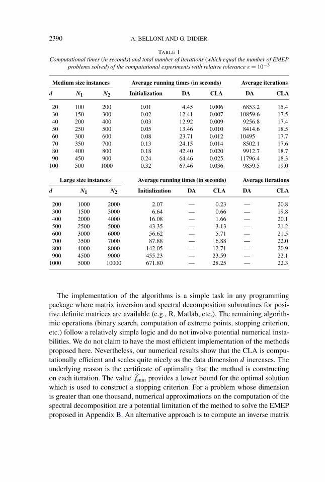
4.2. Computational experiments with CLA and DA. Our complexity boundfor the CLA is worse than that for the DA. However, the DA solves the EMEPfor every point of the discretized domain of u1. In contrast, the CLA seeks toproduce a certificate of ε-optimality at each iteration by comparing the best currentsolution and the solution to the minimization on Kk . In computational practice,this drastically reduces the number of necessary iterations to find an ε-solution,as can be seen in Table 1 (this table was generated in the same way as the MonteCarlo study of the tests sizes, as described in Section 5.2 below). Each entry ofrunning times and iterations in Table 1 is an average over ten instances.

Table 1 reflects the expected computational behavior of the methods. As thedimension increases, more effort is needed but the CLA is order of magnitudesfaster than the DA, since the latter requires the complete discretization of the inter-val [L1,U1]. Such requirement of evaluating the function g on O(1/ε) differentpoints (remember that the complexity analysis is exact in the case of the DA) seemsto be a naive approach, indeed.

The polyhedral approximation used in the CLA provides a way of focusingthe search on a promising region, a concept well exploited in the Optimizationliterature. Table 1 also illustrates the number of loops required by each algorithmin the test problems.

The number of loops performed by the Discretization Algorithm depends onlyon the precision ε, and on the problem dependent values of L1 and U1. On theother hand, these problem dependent quantities do not seem to affect the CLA.This points to the question of whether there exists a (better) complexity analysisfor the CLA which might be independent of these quantities.


TABLE 1Computational times (in seconds) and total number of iterations (which equal the number of EMEP

problems solved) of the computational experiments with relative tolerance ε = 10−3

Medium size instances Average running times (in seconds) Average iterations

d N1 N2 Initialization DA CLA DA CLA

20 100 200 0.01 4.45 0.006 6853.2 15.430 150 300 0.02 12.41 0.007 10859.6 17.540 200 400 0.03 12.92 0.009 9256.8 17.450 250 500 0.05 13.46 0.010 8414.6 18.560 300 600 0.08 23.71 0.012 10495 17.770 350 700 0.13 24.15 0.014 8502.1 17.680 400 800 0.18 42.40 0.020 9912.7 18.790 450 900 0.24 64.46 0.025 11796.4 18.3

100 500 1000 0.32 67.46 0.036 9859.5 19.0

Large size instances Average running times (in seconds) Average iterations

d N1 N2 Initialization DA CLA DA CLA

200 1000 2000 2.07 — 0.23 — 20.8300 1500 3000 6.64 — 0.66 — 19.8400 2000 4000 16.08 — 1.66 — 20.1500 2500 5000 43.35 — 3.13 — 21.2600 3000 6000 56.62 — 5.71 — 21.5700 3500 7000 87.88 — 6.88 — 22.0800 4000 8000 142.05 — 12.71 — 20.9900 4500 9000 455.23 — 23.59 — 22.1

1000 5000 10000 671.80 — 28.25 — 22.3

The implementation of the algorithms is a simple task in any programmingpackage where matrix inversion and spectral decomposition subroutines for posi-tive definite matrices are available (e.g., R, Matlab, etc.). The remaining algorith-mic operations (binary search, computation of extreme points, stopping criterion,etc.) follow a relatively simple logic and do not involve potential numerical insta-bilities. We do not claim to have the most efficient implementation of the methodsproposed here. Nevertheless, our numerical results show that the CLA is compu-tationally efficient and scales quite nicely as the data dimension d increases. Theunderlying reason is the certificate of optimality that the method is constructingon each iteration. The value fmin provides a lower bound for the optimal solutionwhich is used to construct a stopping criterion. For a problem whose dimensionis greater than one thousand, numerical approximations on the computation of thespectral decomposition are a potential limitation of the method to solve the EMEPproposed in Appendix B. An alternative approach is to compute an inverse matrix


at each iteration of the EMEP, which will lead to a more robust implementation atthe cost of additional running time (see [7] for details).

In our experiments we use medium and large size instances where the data di-mension d varies from 20 to 1000. The results were generated using a relativeprecision of ε = 10−3. We report the average over ten different instances. The DAhas proved to be too cumbersome for large instances.

5. Finite sample properties of the Wald, Likelihood Ratio and LagrangeMultiplier tests through the CLA. Three commonly used multivariate testsbased upon the maximization of the log-likelihood function are the Wald (W ),Likelihood Ratio (LR), and the Lagrange Multiplier (LM) Tests. Define θ =(μ1,μ2,�1,�2). For a certain hypothesized restriction on the parameter spaceof means

H0 : c(μ1,μ2) = q,

let θ denote the unrestricted MLE of θ , and let θr denote the MLE under therestriction H0, that is, the solution to the problem

maxθ

l(θ)

subject to c(μ1,μ2) = q.

The test statistics of interest are defined as

W = [c(μ1, μ2) − q]′(Var(c(μ1, μ2) − q

))−1[c(μ1, μ2) − q],LR = −2

(l(θr ) − l(θ )

)and

LM = eT Gr [GTr Gr ]−1GT

r e,

where

Gr = [gx1,r , . . . , g

xN1,r

, gy1,r , . . . , g

yN2,r

]T ,(17)

gxi,r = ∇θr

logf (xi, θr ) and gyi,r = ∇θr

logf (yi, θr ),

(f is the multivariate density function in question) and e is a vector of ones. In thecontext of the BFP, the restriction can be written as μ1 − μ2 = 0 and the W teststatistic has the explicit form

W = (X − Y )′(S1/N1 + S2/N2)−1(X − Y ).

The W Test—which is a pure significance test—bears the computational advantageof not requiring the solution to the problem of finding the restricted MLE estimator(however, see Section 5.2 below).


The W , LR and LM Tests are asymptotically equivalent under the null hypoth-esis. However, their behavior can be rather different in small samples, and theirfinite sample properties are usually unknown, except for a few particular cases(see, e.g., Greene [12] and Godfrey [11]). In this section we use the CLA to inves-tigate and compare the finite sample properties—size and power—of these tests.In particular, we are interested in the sensitivity of the tests to dimensionality.

We emphasize that the CLA allows for the study of the properties of thetests in high-dimensional contexts. In contrast, the literature on the BFP typicallyoverlooks the issue and reports results for small dimensional problems, typicallysmaller than d = 6 and in general no greater than d = 10.

5.1. Conflict among criteria. It is well known that the W , LR and LM statisticsfor testing linear restrictions in the context of classical linear models satisfy theinequalities W ≥ LR ≥ LM (see Savin [25], Berndt and Savin [2], Breusch [4] andGodfrey [11]). Before turning to simulations, we show that such inequalities alsohold in the case of the BFP.

THEOREM 5.1. For the BFP,

W ≥ LR ≥ LM.(18)

PROOF. To show the first inequality, note that, using since log(1 + δ) ≤ δ, wehave

LR ≤ c0 = minμ

N1(X − μ)S−11 (X − μ) + N2(Y − μ)S−1

2 (Y − μ).

The optimal solution of the right-hand side is achieved at μ0 = (N1S−11 +

N2S−12 )−1(N1S

−11 X + N2S

−12 Y ). Using μ0, and the matrix identities

(A + B)−1 = A−1 − A−1(A−1 + B−1)−1A−1 = A−1(A−1 + B−1)−1B−1,

we prove that c0 = (X − Y )′(S1/N1 + S2/N2)−1(X − Y ) = W .

Let μ be a solution for the BFP. After simplifications, the LM statistic can bewritten as

LM = N1(X − μ)′�−11 (X − μ) + N2(Y − μ)′�−1

2 (Y − μ).

Next note that

(X − μ)′�−11 (X − μ) = (X − μ)′S−1

1 (X − μ) − [(X − μ)′S−11 (X − μ)]2

1 + (X − μ)′S−11 (X − μ)

by using a rank-one update formula2 for �−11 . The result follows by considering

the term for Y as well and noting that log(1 + δ) ≥ δ − δ2

1+δ. �

2For invertible M and a vector v, the inverse of the rank-one update of M by vv′ can be written as

(M + vv′)−1 = M−1 − M−1vv′M−1

1+v′M−1v.


5.2. Monte Carlo study of the size of the test. Inequalities (18) imply that therejection rate of the W Test is greater than or equal to that of the LR Test, which inturn is greater than or equal to that of the LM Test. A more accurate understandingof the extent to which this influences the size and the power of such tests can beobtained through simulations.

We performed a Monte Carlo study of the finite-sample properties of the W ,LR and LM tests at sizes α = 0.01,0.05,0.10. The rejection regions were definedbased upon Wilks’ Theorem on the asymptotic χ2

d distribution of the test statistic.The study also includes the Likelihood Ratio statistic with the Bartlett correction

B :=(

1 − c1

N − 2

)LR,

where

c1 = ψ1 − ψ2

d,

ψ1 = N22 (N − 2)

N2(N1 − 1){tr(S1S

−1)}2 + N2

1 (N − 2)

N2(N2 − 1){tr(S2S

−1)}2,

ψ2 = N22 (N − 2)

N2(N1 − 1){tr(S1S

−1S1S

−1)} + N2

1 (N − 2)

N2(N2 − 1){tr(S2S

−1S2S

−1)},

and S = N2N

S1 + N1N

S2.The Bartlett correction as defined above provides an O(N−2) approximation to

the mean of the χ2d distribution (more details can be found in Yanagihara and Yuan

[36]). We will refer to the LR Test under the Bartlett correction as the B Test.To facilitate comparison with other works on the multivariate BFP (e.g., Yao

[37], Subrahmaniam and Subrahmaniam [33], Kim [16] and Krishnamoorthy andYu [18]), we performed tests for the low dimensional cases of d = 2,5 and 10, butwe also included the higher-dimensional cases of d = 25,50,75, 100 and 200. Foreach d , the sample sizes used were N1 = 5d,10d,20d , and N2 = 2N1. For a givendimension size d , each covariance matrix �i , i = 1,2, was constructed by creatingan initial matrix Mi with N(0,1) entries, and then setting �i = MiM

′i .

The results can be seen in Figure 4 (the actual numerical output can be foundin Table 4 in the Appendix D). Each entry was generated using 10,000 runs. TheW and the LR tests tend to over-reject the null hypothesis, while the LM Testtends to slightly under-reject it. We kept constant the ratio between the numberof observations and the dimension so that we can observe how the quality of theapproximation behaves as the dimensionality of the problem grows. One may no-tice how sensitive the W and the LR Tests are to increases in the dimension. Onlyfor the (relatively) large sample case N1 = 20d does the LR Test have actual sizefairly close to α. On the other hand, the W Test appears to demand even (relatively)larger samples. For instance, when d = 100 and α = 0.10, even when N1 = 20d ,


FIG. 4. The behavior of the size of the tests when the dimension increases and the ratio betweenthe number of observations and dimension is fixed.


the W test is off by 3.8 percentage points. The ease of computation of the W teststatistic appears to come at a considerable price in terms of the accuracy of thetest.

In contrast with the W and the LR Tests, the LM shows remarkable robustnesswith respect to dimensionality. For all α, there does not appear to be any clear(say, monotonic) pattern of change on the actual test size with respect to increasesin dimensionality, or maybe even sample size N1.

For all values of α and different sample sizes, the B Test is roughly as accu-rate as the LM Test for low dimensional settings (roughly, d ≤ 20). For d > 20,though, it grossly over-compensates the over-rejection rates of the W Test, withthe possible exception of the comparatively large sample sizes N1 = 20d .

Figure 4 illustrates the above comments. Accordingly, the W Test usuallyshows the steepest curve of dimension versus actual test size for different N1,while the LM Test displays approximately horizontal curves, especially for higher-dimensional settings.

5.3. Monte Carlo study of the power of the test. We performed computationalexperiments on the power of the W , LR, LM and B Tests for the cases of dimensiond = 10,50,100, and sample sizes N1 = 5d , 10d and 20d , with N2 = 2N1.

The analysis of the power for multivariate tests is naturally more difficult dueto the multi-dimensionality of the parameter space. For this reason, we chose toinvestigate and compare the power of the W , LR, LM and B Tests over a standard-ized parameter space in the following sense. For each simulation run, covariancematrices �1 and �2 were (randomly) generated through the same procedure as theone for the evaluation of the sizes of the test. The mean of X, μ1, was set to zeroby default. The choice of the mean(s) of Y , μ2(�), was made as solution(s) to thesquared Mahalanobis distance equation(s)(

μ1 − μ2(�))′(�1 + �2)

−1(μ1 − μ2(�)

) = �2,

where � represents a family of appropriately selected constants. For convenience,such solutions μ2(�) were always taken on some canonical axis, and the specificaxis chosen changed across simulation runs. The use of randomly standardizedMahalonobis distances is justified by the fact that the BFP is defined without in-formation on the population covariances.

The results are depicted in Figure 5, which contains plots for dimensions d =10, 50 and 100. Colors represent tests, while geometric figures represent samplesizes (e.g., a triangle symbolizes N1 = 5d).

Perhaps the most striking feature of all four plots (d = 10, 50 and 100) is the factthat, for a given sample size N1, the shapes of the power curves for the four testslook alike. More specifically, given N1, the curve for the W Test looks like an up-shifted version of the curve for the LR Test, which in turn looks like an up-shiftedversion of the curve for the LM Test. The same is true for the curve for the B Test,which lies mostly below the curve for the latter. The observed “order” of the curves


FIG. 5. Monte Carlo study of the power of the W , LR, LM and B Tests for the size α = 0.05 withdifferent sample sizes and dimensions equal to 10, 50 and 100.


should not come as a surprise. First, regarding the W , LR and LM Tests, because ofthe theoretical inequalities in Theorem 5.1. Second, because the simulation resultsfor the test sizes show that the W and LR Tests tend to over-reject the null hypoth-esis (the former, substantially more than the latter), while the LM Test has sizeclose to α and the B Test tends to under-reject the null hypothesis. In other words,we are essentially comparing tests of different sizes (see also the conclusions inBreusch [4] for the case of linear regression). The shape of the curves suggests thepossibility that, if test size adjustment is made for the W and LR Tests, the powercurves of the three tests may get rather close to each other. Such adjustment wouldimply, of course, going beyond Wilks’ Theorem and developing exact quantiles,especially for the W and the LR Tests.

The plot for the low-dimensional case of d = 10 displays a “well-behaved” pat-tern, in the sense that the curves for different tests and for the same sample sizetend to be grouped together. In particular, the curves for sample size N1 = 40d arealmost super-imposed, which means that, power-wise, the tests are nearly equiva-lent in this situation. Note that the curves for sample size N1 = 10d (triangle) lieabove the remaining ones close to the origin, that is, in the case where the Ma-halanobis distance between μ1 and μ2 is small. Again, this should not come as asurprise, since the simulation results for the test sizes (i.e., zero Mahalanobis dis-tance between μ1 and μ2) show that relatively small sample sizes imply a tendencyfor over-rejection in the case of the W and LR Tests.

The effect of higher dimensionality can be seen in the two remaining plots (d =50 and 100). The main impact seems to be greater vertical distances among thecurves for the four tests, particularly for the cases of smaller sample sizes. Evenfor the higher-dimensional case d = 100, though, the larger sample size N1 = 20d

brings the curves a lot closer to each other. As one might expect, larger samplesizes compensate for high dimension and point to the asymptotic equivalence ofthe W , LR, LM and B Tests.

5.4. Performance of local methods/heuristics. Up to the present, the numer-ical procedures applied to the multivariate Behrens–Fisher Problem have beenheuristics or locally convergent methods. Since the CLA is a provably convergentmethod that constructs a certificate of global optimality, it provides a benchmarkfor the previous approaches. So, we are now able to address via Monte Carlo ex-periments the statistically important question of the performance of the LR Testsbased on some widely used heuristics vis-a-vis the LR Test based on the CLA.Also, we are interested in the partially related issue the computational performanceof these heuristics vis-a-vis the CLA.

There is a variety of different heuristics and it is usually hard (if not impossible)to make any general statement about them. However, in the case of the Behrens–Fisher Problem, we do have a “natural” initial point for these algorithms, that is,μ0 := (N1S

−11 + N2S

−12 )−1(N1S

−11 X + N2S

−12 Y ). In fact, μ0 is at the same time:

(i) from the algorithmic perspective, the solution to the first-order conditions of the


objective function (the log-likelihood) with respect (only) to μ, after we substituteSi for �i , i = 1,2; (ii) from the statistical perspective, the estimator of the meanμ associated with the W statistic. Also, by the proof of Theorem 5.1, we have

W ≥ LR0 ≥ LR,(19)

where LR0 is the log-likelihood ratio evaluated at μ0. Denote by LRh the (po-tentially suboptimal) Likelihood Ratio test statistic based upon a given heuristicmethod and with μ0 as its initial point. We can assume (through an ad-hoc modi-fication of the heuristic, if necessary) that

LR0 ≥ LRh.(20)

Thus, by (19), (20) and the fact that LRh ≥ LR, the statistic LRh also asymptoticallyfollows a χ2

d distribution. Nonetheless, the gap between the W and the LR statisticscan be quite large in finite-samples (see Section 5).

Note that a LRh Test can only disagree with the LR Test if the LR0 Test rejectsH0 and the latter accepts H0. We can perform Monte Carlo experiments (in thesame way as in Section 5.2 for the tests sizes) to estimate how often the LR0 andLR Tests disagree. By (20), this provides a guarantee (i.e., an upper-bound) on the“discrepancy rate” between a LRh Test (i.e., based on any heuristic) and the LRTest. The results in Table 2 show that this worst-case-scenario discrepancy rateis surprisingly small. The discrepancy rate for the W Test with respect to the LRTest—substantially higher—was also included for the sake of comparison.

Next we study the computational performance of three commonly used meth-ods: Simulated Annealing (SA), Iterative Update (ItUp) and Newton’s Methodwith Line Search (NM). (See, resp., [17, 19], [5] and [7] for discussions and im-plementation details of these methods.)

Table 3 reports the average performance of the heuristics with respect to runningtimes, iterations and discrepancy rate based on their respective LRh Tests. As ex-pected, the discrepancy rate is smaller than in Table 2, since the heuristics usuallyprovide a solution superior to μ0. Not only that, the experiments suggest that bothItUp and NM are robust in terms of discrepancy rate (with μ0 as the initial point)

TABLE 2Monte Carlo study of the discrepancy rates for LR0 and W Tests with respect to the LR Test fordifferent dimensions d (for each entry, simulations were run until 50 “successes” were obtained)

d 2 5 10 20 30 40LR0 0.00176 0.00113 0.000932 0.000978 0.000825 0.00135W 0.0299 0.0325 0.0261 0.0468 0.0342 0.0513

d 50 60 70 80 90 100LR0 0.0009 0.0012 0.0012 0.0013 0.0017 0.0012W 0.0426 0.0702 0.0641 0.0796 0.0809 0.0935


TABLE 3The average performance of heuristics averaged over 5000 runs: time (seconds), iterations and

discrepancy rate

Algorithms

SA ItUp NM

d Time Iter Discrep Time Iter Discrep Time Iter Discrep

2 0.02462 1000 0.001 0.00062 4.2 0 0.00118 2.3 05 0.02547 1000 0.001 0.00081 4.5 0 0.00135 2.6 0

10 0.02680 1000 0.001 0.00121 4.7 0 0.00166 2.6 020 0.03120 1000 0.001 0.00273 5.0 0 0.00310 2.7 030 0.04078 1000 0.001 0.00799 5.1 0 0.00662 2.9 040 0.04948 1000 0.001 0.00879 5.4 0 0.00787 3.1 050 0.06037 1000 0.001 0.01339 5.3 0 0.01179 3.0 060 0.07422 1000 0.001 0.01998 5.3 0 0.01726 3.0 070 0.09325 1000 0.001 0.03057 5.3 0 0.02537 3.0 080 0.11258 1000 0.003 0.04069 5.5 0 0.03408 3.1 090 0.13279 1000 0.001 0.05461 5.5 0 0.04414 3.0 0

100 0.16051 1000 0.001 0.07260 5.9 0 0.05852 3.5 0

even though they can be trapped in local minima. Moreover, their good (local)convergence properties are illustrated by the notably small number of iterations.On the other hand, SA seems to have trouble achieving local convergence, and itsgood performance with respect to errors appears to be a by-product of the choseninitial point. Not surprisingly, the convergence of the CLA turned out to be slower(i.e., larger number of iterations) than the local methods ItUp and NM. In fact, oneshould keep in mind that the CLA aims not only to find a good solution, but also toconstruct a certificate of global optimality, which is a much harder task. Regardingrunning time, the main computational cost of CLA is the spectral decompositionat initialization (see Table 1). The running time of the CLA after initialization isactually faster than SA, ItUp and NM at higher dimensions (cf. Tables 1 and 3).

We now make a few quick remarks regarding the implementation of the meth-ods. First, all methods do require a matrix inversion routine: SA and CLA, onlyon the first iteration; ItUp and NW, on every iteration. Second, in contrast to CLA,ItUp and NW, the calibration of additional parameters is needed for the SA. Third,the implementation of SA and ItUp is very simple, while the Line Search for NMis slightly more difficult. Fourth, unlike the other methods, the CLA involves theadditional implementation costs associated with the optimality certificate basedon Kk , and with the spectral decomposition of a positive definite matrix (see alsoSection 4.2).

6. Extension to Behrens–Fisher-like Problems. It should be noted that themethodology proposed in this paper can be applied to a much broader class of


problems. Strictly speaking, all we need is to be able to replicate the strategy ofconstructing lifted problems whose solution lie on extreme points of a two dimen-sional convex domain,3 and to evaluate the subproblems which define the convexdomain. A sufficient condition for this is the quasi-concavity of the objective func-tion of the lifted problem and the convexity of the subproblems.

To set up a broader framework, assume we have two random samples {Xi}N1i=1

and {Yi}N2i=1 whose log-likelihood functions are denoted by l1(X;μ,α) and

l2(Y ;μ,β), respectively. The generalized M-estimation problem of interest is de-fined as

maxμ,α,β

l1(X;μ,α) + l2(Y ;μ,β).

A generalization of the subproblem can be cast in terms of the log-likelihoodfunctions directly. Assume there exist two monotone (decreasing) transformationsTX,TY : R → R such that TX(l1(X; ·, ·)) and TY (l2(Y ; ·, ·)) are convex functions.The subproblems, analogous to the EMEP, are

hX(u1) = minμ,α,β

{TY (l2(Y ;μ,β)) :TX(l1(X;μ,α)) ≤ u1}.The geometric results in Section 3 still hold with minor modifications. Moreover,under the above convexity assumption, the evaluation of hX(u1) can be efficientlyperformed through standard convex programming techniques. Therefore, the con-vergence results of Section 4 are still valid.

The above framework encompasses the BFP by taking TX(z) = exp( 2N1

z) − 1

and TY (z) = exp( 2N2

z) − 1.We now give a simple example of the application of the methodology described

above to a Behrens–Fisher-like Problem.

EXAMPLE 6.1. Assume X ∼ N(μ,�) but, differently from the BFP, Y fol-lows a multivariate Laplacian distribution, that is,

fY (y) = cL exp(−‖y − μ‖),where cL is the normalization constant and ‖ · ‖ is the Euclidean norm. The relatedlifted problem can be cast as

minμ,u1,u2

f (u1, u2) = N1

2log(u1) + u2,

u1 ≥ 1 + MX(μ),(21)

u2 ≥N2∑i=1

‖Yi − μ‖.

3Higher-dimensional convex domains would impose an additional burden in terms of computa-tional complexity.


Here, the problem objective function is concave (u1, u2), and therefore the solutionmust lie on the border of the convex domain of these variables. Such a domain canbe written as

K =⎧⎪⎨⎪⎩ (u1, u2) ∈ R

2 :∃μ such that

u1 ≥ 1 + MX(μ)

u2 ≥ 1 +N2∑i=1

‖Yi − μ‖

⎫⎪⎬⎪⎭ .(22)

Moreover, the associated subproblems, using TX(z) = exp( 2N1

z)−1 and TY (z) = z,are convex programming problems and have the form

hX(u1) = minμ

{N2∑i=1

‖Yi − μ‖ :MX(μ) ≤ u1

}

and

hY (u2) = minμ

{MX(μ) :

N2∑i=1

‖Yi − μ‖ ≤ u2

}.

Both these problems can be solved via convex quadratic programming, which canbe done quite efficiently even in high-dimensional cases.

APPENDIX A: NOTATION OF CONVEX ANALYSIS

Herein we gather the definitions of relevant concepts in Convex Analysis forthis work. We refer to [24] for an analytic exposition of Convex Analysis and to[13] for a more geometric one.

A set S is convex if, for any x, y ∈ S, α ∈ [0,1], αx + (1−α)y ∈ S. An extremepoint of a convex set is a point that cannot be written as a strictly (α < 1) convexcombination of any other distinct points in the set. A set P is said to be polyhedralif P = {x ∈ R

n :Ax ≤ b}, where A is a matrix, and b, a vector. It follows thatpolyhedral sets are convex and their extreme points are its corners. The recessioncone CS of a convex set S is the set of directions that go to infinity in S, formally,CS = {d :d + S ⊂ S}.

A function g : Rn → R is said to be convex if, for any x, y ∈ Rn, and α ∈ [0,1],

g(αx + (1−α)y) ≤ αg(x)+ (1−α)g(y). A function f : Rn → R is quasi-concaveif, for any x, y ∈ R

n, and α ∈ [0,1], f (αx + (1 − α)y) ≥ min{f (x), f (y)}, orequivalently, the upper level sets of f are convex sets.

Given a convex function g : Rn → R, we can define its subdifferential at x as∂g(x) = {s ∈ R

n :g(y) ≥ g(x) + 〈s, y − x〉, for all y ∈ Rn}. The elements of the

subdifferential, also called subgradients, play the role of the gradient in case g isnondifferentiable. Note that ∂g(x) is always nonempty.


APPENDIX B: SOLVING THE EMEP

Consider the convex problem in (7). There are a variety of “general purpose”convergent algorithms that can solve it. Here, we propose a specific algorithmtailored for the particular structure of the EMEP.

Let λ be the (nonnegative) Lagrange multiplier associated with the inequalityconstraint. The first order conditions are necessary and sufficient, and are given by

2S−12 (Y − μ) + 2λS−1

1 (X − μ) = 0

and

λ(MX(μ) − v1

) = 0.

Assuming that λ > 0 (otherwise, the solution is just μ = Y ), the optimal μ is afunction only of λ:

μ(λ) = (S−12 + λS−1

1 )−1(S−12 Y + λS−1

1 X).(23)

Therefore, in order to solve the EMEP, it suffices to compute a root λ∗ of thenonlinear univariate function

m(λ) = MX(μ(λ)) − v1.(24)

The algorithm we propose here is based upon the algorithm in Ye [38], who inturn built upon earlier work by Smale [29].

Our algorithm is made up of two main parts. The first part consists of a binarysearch over intervals of increasing length to find which interval Ii∗ contains whatSmale [29] calls an approximate root.

DEFINITION B.1. A point λ0 is said to be an approximate root of an analyticreal function m : R → R if

|λk+1 − λk| ≤ (1/2)2k−1−1|λ1 − λ0|.In the second part of the algorithm, Newton’s method is used over the interval

Ii∗ to find the approximate root λ∗. For the sake of exposition, we focus on thecase of m : R → R (the results in [38] hold in much greater generality, though).Recall that the Newton iterate for a function m from a current point λk is

λk+1 = λk − m(λk)

m′(λk+1).

Newton’s Method (NM) converges quadratically from the very first iteration. In[29], Smale gives sufficient conditions under which a particular point is an approx-imate root. Although it is hard to verify Smale’s condition in general, Ye provideda constructive method to find such a point for a particular class of functions. Ye’sresults in [38] apply in our case. We now write out Ye’s algorithm and prove acomplexity result for it in the context of the BFP.


Binary Search and Newton Method

Input: Upper and lower bounds on the value of the root [a, b], b ≥ a ≥ δ,tolerance δ > 0.

Step 1. Define a partition of [a,b] through intervals of the form

Ii = [a(1 + 1/12)i, a(1 + 1/12)i+1).Step 2. Perform binary search on these intervals to find Ii∗

that contains the true root λ∗.

Step 3. Let λ0 = a(1 + 1/12)i , k = 0.

Step 4. Perform Newton’s method from λk: λk+1 ← λk − m(λk)

m′(λk).

Step 5. Stop if k > 1 + log2(1 + max{0, log2(b/δ)}) steps.

Step 6. Else set k ← k + 1, and goto Step 4.

THEOREM B.1. After the computation of a spectral decomposition of the ma-trix S

1/21 S−1

2 S1/21 , and given a desired precision δ > 0 and an upper bound b for

the solution, the algorithm finds a δ-approximate solution λ such that |λ∗ − λ| < δ

in at most

O

(d log log

b

δ

)arithmetic operations.

PROOF. Making the following change of variables/notation

w := S−1/21 (μ − X), M := S

1/21 S−1

2 S1/21 = PDPT ,

v = 2S−12 S

1/21 (Y − X) and s = P T v,

problem (15) is equivalent to

h(v1) = minwT Mw − vT w,

‖w‖2 ≤ v1

up to a constant value (which does not matter for the optimization).Under the new notation, we can rewrite the function m as

m(λ) = sT (D + λI)−2s − v1 =d∑

i=1

s2i

(Di + λ)2 − v1.

The function m(λ) is analytic and its derivatives can be easily computed as

m(k)(λ) = (−1)k(k + 1)!d∑

i=1

s2i

(Di + λ)k+2 .


Note that m′ < 0 and m′′ > 0 (i.e., m is decreasing and convex). Thus, we canevaluate m and m′ in O(d) operations. This implies that each Newton step can beimplemented in O(d) arithmetic operations.

Let λ0 = a(1 + 1/12)i∗

be the left endpoint of the interval selected by binarysearch. From Ye [38], it follows that λ0 satisfies Smale’s sufficient condition to bean approximate root. Therefore, NM converges quadratically from the very first it-eration (i.e., from λ0). From the convexity of m, the convergence is monotone, thatis, 0 < λ0 < λk < λk+1 < λ∗ ≤ b for every k (in particular, we have |λ1 − λ0| < b).This implies that we need at most

k = 1 + log2(1 + max{0, log2(b/δ)})

Newton steps to achieve |λk − λ∗| < δ. Moreover, the total number of subin-tervals is 1

log(1+1/12)log(b/a). The binary search can thus be implemented in

O(log log(b/a)). The result follows by noting that we can take a ≥ δ. �

REMARK B.1. Even when we need to solve the EMEP for many differ-ent levels of the Mahalanobis distance function, the spectral decomposition ofS

1/21 S−1

2 S1/21 needs to be performed only once. This feature of the algorithm makes

it a good auxiliary method for the CLA.

The following lemma illustrates how to obtain subgradients for the function hX

with no additional computational effort, which is of interest for the CLA.

LEMMA B.1. Let λ∗ be a root of the function m as defined in (24). Then −λ∗is a subgradient of hX at v1.

PROOF. Recall m(λ∗) = 0 implies that μ(λ∗) minimizes MY (μ)+λ∗MX(μ).For any v, we have

hX(v1) = MY (μ(λ∗)) = MY (μ(λ∗)) + λ(MX(μ(λ∗)) − v1

)= MY (μ(λ∗)) + λ∗(

MX(μ(λ∗)) − v) + λ∗(v − v1)

≤ hX(v) + λ∗(v − v1).

Here, we used weak duality (min max ≥ max min) as follows:

hX(v) = minμ

maxλ≥0

MY (μ) + λ(MX(μ) − v

)≥ max

λ≥0min

μMY (μ) + λ

(MX(μ) − v

)≥ MY (μ(λ∗)) + λ∗(

MX(μ(λ)) − v).


Therefore, for every v, we have

hX(v1) − λ∗(v − v1) ≤ hX(v),

which implies that −λ∗ ∈ ∂hX(v1). �

APPENDIX C: THE DISCRETIZATION ALGORITHM (DA)

Consider the problem (5) for a fixed value of u1 = u1. In this case, the compu-tational problem reduces exactly to solving the EMEP with respect to X at a fixedsquared distance level u1 −1. As shown in Section 2, such a problem can be solveddirectly with the algorithm proposed in Appendix B.

Therefore, given the desired precision, one can discretize the range of the vari-able u1, [L1, U1], and solve the EMEP for each one of these values. Such a schemeyields the following algorithm.

Discretization Algorithm

Input: Relative tolerance ε > 0, u11 = (1 + 2ε/N1)L1, k = 1.

Step 1. Evaluate uk2 = g(uk

1) and compute f k = N12 log(uk

1) + N22 log(uk

2).

Step 2. If (1 + 2ε/N1)uk1 > U1, compute f k+1 = U1L2, goto Step 4.

Step 3. Else set uk+11 ← (1 + 2ε/N1)u

k1, k ← k + 1, goto Step 1.

Step 4. Report min1≤i≤k f i and the correspondent pair (ui∗1 , ui∗

2 ).

The following complexity result holds for the Discretization Algorithm.

THEOREM C.1. The Discretization Algorithm reports an ε-solution for theoriginal problem after exactly �log(U1/L1)/ log(1 + 2ε/N1)� loops.

PROOF. Let u∗ = (u∗1, u

∗2) be a optimal solution. There exists a k such that

uk1 < u∗

1 < (1 + 2ε/N1)uk1. We consider f k+1 as our candidate. We have

f ∗ = N1

2log(u∗

1) + N2

2log(u∗

2)

≤ f k+1 = N1

2log(1 + 2ε/N1) + N1

2log(uk

1) + N2

2log(uk+1

2 )(25)

≤ ε + N1

2log(uk

1) + N2

2log(uk+1

2 ) = ε + f ∗,

where we also used that uk+12 ≤ u∗

2, since g in (14) is decreasing.The claim on the number of loops follows by noting that we have uk

1 = L1(1 +2ε/N1)

k ≤ U1 and by taking logs to bound k. �By choosing a sequence εk → 0, we obtain a sequence of εk-solutions that con-

verge to the optimal solution of the BFP. One drawback to this method is that it


requires solving the EMEP at every point of the discretization. In practice, suchrequirement may be cumbersome.

APPENDIX D: MONTE CARLO STUDY OF SIZE

TABLE 4Monte Carlo study of size for the W , LR, LM and B Tests (runs per entry = 10,000)

Small sizeinstances

Size of the Test α

α = 0.10 α = 0.05 α = 0.01

d N1 N2 W LR LM B W LR LM B W LR LM B

2 10 20 0.160 0.133 0.102 0.092 0.106 0.077 0.046 0.046 0.039 0.020 0.005 0.0092 20 40 0.138 0.122 0.106 0.103 0.081 0.067 0.050 0.051 0.023 0.013 0.007 0.0092 40 80 0.120 0.114 0.110 0.107 0.069 0.061 0.055 0.054 0.017 0.014 0.011 0.0115 25 50 0.171 0.133 0.098 0.090 0.101 0.073 0.047 0.046 0.035 0.019 0.005 0.0085 50 100 0.124 0.110 0.094 0.090 0.068 0.055 0.041 0.041 0.017 0.011 0.007 0.0085 100 200 0.113 0.106 0.098 0.096 0.063 0.057 0.053 0.052 0.015 0.013 0.010 0.010

10 50 100 0.175 0.131 0.094 0.084 0.102 0.072 0.044 0.041 0.035 0.018 0.008 0.00810 100 200 0.137 0.118 0.099 0.093 0.074 0.062 0.047 0.047 0.019 0.012 0.009 0.00910 200 400 0.116 0.107 0.100 0.098 0.062 0.056 0.051 0.051 0.014 0.011 0.009 0.009

Medium sizeinstances

Size of the Test α

α = 0.10 α = 0.05 α = 0.01


25 125 250 0.196 0.141 0.096 0.077 0.118 0.079 0.043 0.034 0.035 0.018 0.007 0.00725 250 500 0.137 0.109 0.088 0.078 0.071 0.056 0.039 0.036 0.019 0.014 0.008 0.00725 500 1000 0.120 0.110 0.099 0.091 0.064 0.055 0.049 0.046 0.015 0.011 0.009 0.00850 250 500 0.232 0.158 0.096 0.065 0.144 0.089 0.040 0.027 0.041 0.018 0.005 0.00550 500 1000 0.147 0.117 0.091 0.079 0.083 0.061 0.044 0.038 0.021 0.013 0.008 0.00750 1000 2000 0.126 0.111 0.100 0.092 0.070 0.062 0.053 0.049 0.016 0.012 0.011 0.01075 375 750 0.262 0.170 0.098 0.064 0.167 0.098 0.048 0.029 0.059 0.025 0.008 0.00475 750 1500 0.166 0.131 0.097 0.084 0.098 0.072 0.048 0.038 0.025 0.016 0.009 0.00775 1500 3000 0.133 0.119 0.102 0.092 0.073 0.064 0.053 0.049 0.018 0.014 0.010 0.009

100 500 1000 0.284 0.175 0.090 0.054 0.179 0.097 0.043 0.025 0.060 0.025 0.007 0.004100 1000 2000 0.175 0.134 0.101 0.076 0.104 0.071 0.047 0.036 0.026 0.016 0.008 0.006100 2000 4000 0.139 0.117 0.099 0.087 0.073 0.061 0.050 0.042 0.017 0.013 0.009 0.007

Large sizeinstances

Size of the Test α

α = 0.10 α = 0.05 α = 0.01


200 1000 2000 0.373 0.213 0.095 0.040 0.251 0.123 0.043 0.015 0.101 0.030 0.007 0.002200 2000 4000 0.203 0.136 0.085 0.060 0.112 0.073 0.042 0.029 0.032 0.016 0.009 0.005200 4000 8000 0.153 0.128 0.099 0.085 0.084 0.064 0.049 0.039 0.019 0.014 0.010 0.007


Acknowledgments. We are grateful to Victor Chernozhukov, Donald Richardsand Vladas Pipiras for thoroughly reading preliminary versions of this paper, andto Pierre Bonami, Oktay Günlük, Jon Lee, Katya Scheinberg and Andreas Wächerfor useful discussions. We also thank two anonymous referees and the associatededitor for their comments that helped improve the paper.

REFERENCES

[1] BEHRENS, W. (1929). Ein beitrag zur fehlerberechnung bei wenigen beobachtungen [a con-tribution to error estimation with few observations]. Landwirtschaftliche Jahrbücher 68807–837.

[2] BERNDT, E. and SAVIN, N. E. (1977). Conflict among criteria for testing hypothesis in themultivariate linear regression model. Econometrica 45 1263–1278. MR0501583

[3] BONNANS, J. F., GILBERT, J. C., LEMARÉCHAL, C. and SAGASTIZÁBAL, C. A. (2003).Numerical Optimization. Springer, Berlin. MR1958119

[4] BREUSCH, T. S. (1979). Conflict among criteria for testing hypothesis: Extensions and com-ments. Econometrica 47 203–208. MR0518833

[5] BUOT, M.-L. G. and RICHARDS, D. S. P. (2007). Counting and locating the solutions ofpolynomial systems of maximum likelihood equations. II. The Behrens–Fisher Problem.Statist. Sinica 17 1343–1354.

[6] CHIEN, J.-T. (2005). Decision tree state tying using cluster validity criteria. IEEE Trans.Speech Trans. Audio Processing 13 182–193.

[7] CONN, A. R., GOULD, N. I. M. and TOINT, P. L. (2000). Trust-Region Methods. SIAM,Philadelphia, PA. MR1774899

[8] COX, D. R. (1984). Effective degrees of freedom and the likelihood ratio test. Biometrika 71487–493. MR0775394

[9] FISHER, R. A. (1935). The fiducial argument in statistical inference. Ann. Eugenics 6 391–398.[10] FISHER, R. A. (1939). The comparison of samples with possibly unequal variances. Ann. Eu-

genics 9 174–180.[11] GODFREY, L. G. (1988). Misspecification Tests in Econometrics. Cambridge Univ. Press.[12] GREENE, W. H. (1997). Econometric Analysis, 3rd ed. Prentice-Hall Inc., Upper Saddle River,

NJ.[13] HIRIART-URRUTY, J.-B. and LEMARÉCHAL, C. (1993). Convex Analysis and Minimization

Algorithms. Springer, Berlin.[14] KELLEY, J. E. (1960). The cutting plane method for solving convex programs. J. Soc. Indust.

Appl. Math. 8 703–712. MR0118538[15] KIM, S.-H. and COHEN, A. (1998). On the Behrens–Fisher Problem: A review. J. Educational

and Behavioral Statist. 23 356–377.[16] KIM, S.-J. (1992). A practical solution to the multivariate Behrens–Fisher Problem. Biometrika

79 171–176. MR1158525[17] KIRKPATRICK, S. GELATT JR. C. D. and VECCHI, M. P. (1983). Optimization by simulated

annealing. Science 220 671–680. MR0702485[18] KRISHNAMOORTHY, K. and YU, J. (2004). Modified Nel and Van der Merwe test for the

multivariate Behrens–Fisher Problem. Statist. Probab. Lett. 66 161–169. MR2029731[19] LAARHOVEN, P. J. M. and AARTS, E. H. L. (1987). Simulated Annealing: Theory and Appli-

cations. Kluwer Academic Publishers, Norwell, MA.[20] MARDIA, K. V., KENT, J. T. and BIBBY, J. M. (1979). Multivariate Analysis. Academic

Press, New York.[21] MURPHY, B. J. (1987). Selecting out of control variables with the T 2 multivariate quality

control procedure. The Statistician 36 571–581.

http://www.ams.org/mathscinet-getitem?mr=0501583










[22] NESTEROV, Y. and NEMIROVSKII, A. (1994). Interior Point Polynomial Algorithms in ConvexProgramming. SIAM, Philadelphia, PA. MR1258086

[23] ROBBINS, H., SIMONS, G. and STARR, N. (1967). A sequential analogue of the Behrens–Fisher Problem. Ann. Math. Statist. 38 1384–1391. MR0214235

[24] ROCKAFELLAR, R. T. (1970). Convex Analysis. Princeton Univ. Press. MR0274683[25] SAVIN, N. E. (1976). Conflict among testing procedures in a linear regression model with

autoregressive disturbances. Econometrica 44 1303–1315. MR0464507[26] SCHEFFÉ, H. (1943). On solutions of the Behrens–Fisher Problem, based on the t-distribution.

Ann. Math. Statist. 14 35–44. MR0007961[27] SCHEFFÉ, H. (1970). Practical solutions of the Behrens–Fisher Problem. J. Amer. Statist. As-

soc. 65 1501–1508. MR0273732[28] SCHRAMM, C., RENN, S. and BILES, B. (1986). Controlling hospital cost inflation: New

perspectives on state rate setting. Health Affairs Fall 22–33.[29] SMALE, S. (1986). Newton’s method estimates from data at one point. In The Merging of

Disciplines: New Directions in Pure, Applied, and Computational Mathematics (Laramie,Wyo., 1985) 185–196. Springer, New York. MR0870648

[30] SRIVASTAVA, M. S. (2007). Multivariate analysis with fewer observations than the dimension:A review. Preprint. Available at http://www.utstat.utoronto.ca/%7Esrivasta/.

[31] SRIVASTAVA, M. S. (2007). Multivariate theory for analyzing high-dimensional data. J. JapanStatist. Soc. To appear.

[32] STUART, A. and ORD, J. K. (1994). Kendall’s Advanced Theory of Statistics, 6th ed. EdwardArnold, London.

[33] SUBRAHMANIAM, K. and SUBRAHMANIAM, K. (1973). On the multivariate Behrens–Fisherproblem. Biometrika 60 107–111. MR0334413

[34] WELCH, B. L. (1938). The significance of the difference between two means when the popu-lation variances are unequal. Biometrika 29 350–362.

[35] WELCH, B. L. (1947). The generalization of ‘Student’s’ problem when several different popu-lation variances are involved. Biometrika 34 28–35. MR0019277

[36] YANAGIHARA, Y. and YUAN, K.-H. (2005). Three approximate solutions to the multivariateBehrens–Fisher Problem. Comm. Statist.—Simul. Comput. 34 975–988. MR2224272

[37] YAO, Y. (1965). An approximate degrees of freedom solution to the multivariate Behrens–Fisher Problem. Biometrika 52 139–147. MR0221660

[38] YE, Y. (1992). A new complexity result on minimization of a quadratic function with a sphereconstraint. In Recent Advances in Global Optimization (C. Floudas and P. Pardalos, eds.)19–31. Princeton Univ. Press.

THE FUQUA SCHOOL OF BUSINESS

DUKE UNIVERSITY

1 TOWERVIEW ROAD

PO BOX 90120DURHAM, NORTH CAROLINA 27708-0120USAE-MAIL: [email protected]

MATHEMATICS DEPARTMENT

TULANE UNIVERSITY

6823 ST. CHARLES AVENUE

NEW ORLEANS, LOUISIANA 70118USAE-MAIL: [email protected]








http://www.utstat.utoronto.ca/%7Esrivasta/





mailto:[email protected]

mailto:[email protected]

Documents

On the Behrens-Fisher problem: A globally convergent