Embed Size (px)
Citation preview
On the Approximability of Injective Tensor Norm
Vijay Bhattiprolu
CMU-CS-19-115
June 28, 2019
School of Computer ScienceCarnegie Mellon University
Pittsburgh, PA 15213
Thesis Committee:Venkatesan Guruswami, Chair
Anupam GuptaDavid Woodruff
Madhur Tulsiani, TTIC
Submitted in partial fulfillment of the requirementsfor the degree of Doctor of Philosophy.
Copyright c© 2019 Vijay Bhattiprolu
This research was sponsored by the National Science Foundation under awardCCF-1526092, and by the National Science Foundation under award 1422045. The viewsand conclusions contained in this document are those of the author and should not be
interpreted as representing the official policies, either expressed or implied, of anysponsoring institution, the U.S. government or any other entity.

Keywords: Injective Tensor Norm, Operator Norm, Hypercontractive Norms, Sum of SquaresHierarchy, Convex Programming, Continuous Optimization, Optimization over the Sphere,Approximation Algorithms, Hardness of Approximation
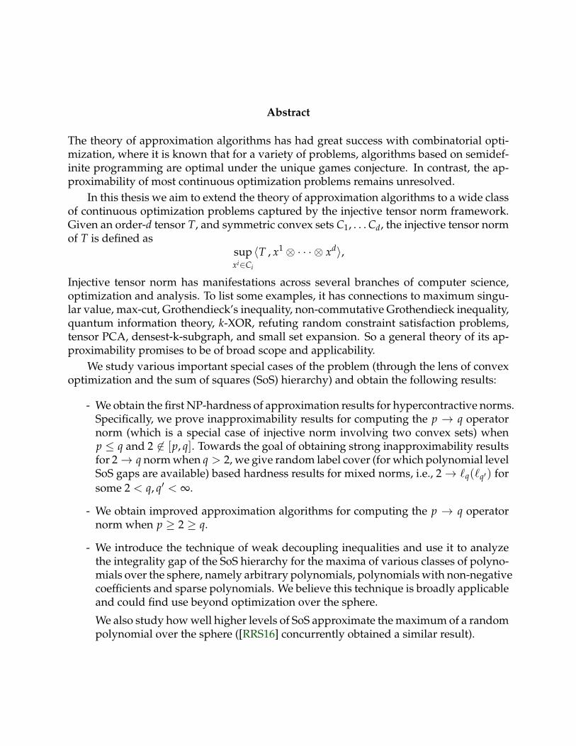
Abstract
The theory of approximation algorithms has had great success with combinatorial opti-mization, where it is known that for a variety of problems, algorithms based on semidef-inite programming are optimal under the unique games conjecture. In contrast, the ap-proximability of most continuous optimization problems remains unresolved.
In this thesis we aim to extend the theory of approximation algorithms to a wide classof continuous optimization problems captured by the injective tensor norm framework.Given an order-d tensor T, and symmetric convex sets C1, . . . Cd, the injective tensor normof T is defined as
supxi∈Ci
〈T , x1 ⊗ · · · ⊗ xd〉,
Injective tensor norm has manifestations across several branches of computer science,optimization and analysis. To list some examples, it has connections to maximum singu-lar value, max-cut, Grothendieck’s inequality, non-commutative Grothendieck inequality,quantum information theory, k-XOR, refuting random constraint satisfaction problems,tensor PCA, densest-k-subgraph, and small set expansion. So a general theory of its ap-proximability promises to be of broad scope and applicability.
We study various important special cases of the problem (through the lens of convexoptimization and the sum of squares (SoS) hierarchy) and obtain the following results:
- We obtain the first NP-hardness of approximation results for hypercontractive norms.Specifically, we prove inapproximability results for computing the p → q operatornorm (which is a special case of injective norm involving two convex sets) whenp ≤ q and 2 6∈ [p, q]. Towards the goal of obtaining strong inapproximability resultsfor 2→ q norm when q > 2, we give random label cover (for which polynomial levelSoS gaps are available) based hardness results for mixed norms, i.e., 2→ `q(`q′) forsome 2 < q, q′ < ∞.
- We obtain improved approximation algorithms for computing the p → q operatornorm when p ≥ 2 ≥ q.
- We introduce the technique of weak decoupling inequalities and use it to analyzethe integrality gap of the SoS hierarchy for the maxima of various classes of polyno-mials over the sphere, namely arbitrary polynomials, polynomials with non-negativecoefficients and sparse polynomials. We believe this technique is broadly applicableand could find use beyond optimization over the sphere.
We also study how well higher levels of SoS approximate the maximum of a randompolynomial over the sphere ([RRS16] concurrently obtained a similar result).

Acknowledgements
First and foremost I would like to thank my parents and sister for their undying support andpatience. I owe a great deal to both of my grandfathers for encouraging me on my path andteaching me in my early years.
I am most fortunate to have been advised by Venkat Guruswami. As all of his students wouldconfirm, he adapts to the needs of his students and I can’t think of anything I wish he did differ-ently. He has been an excellent collaborator: he had troves of questions relevant to my backgroundand interests and would constantly make prescient comments about my research directions. Anyconfidence I have in being able to survive outside the nest, I owe to Venkat’s style of advisory.
I spent two wonderful summers (and more) at TTI chicago hosted by Madhur Tulsiani. Mad-hur has always been incredibly generous with his time and knowledge, and has been virtually asecond advisor to me. Thanks Madhur!
I greatly enjoyed my collaboration and friendship with Euiwoong and Mrinal. I’ve learned somuch from both of them and I look forward to our collaborations for years to come.
I am very grateful to Assaf Naor, Prasad Raghavendra and Pravesh Kothari for their insightfuland influential comments on my research directions. Special thanks to Prasad for hosting me atBerkeley for a few months.
I’d like to thank my committee (Venkat, Madhur, David Woodruff and Anupam Gupta) fortaking the time and giving me valuable comments. My gratitude to Anupam, Danny and Davidfor helping with Ph.D. program requirements.
Ryan and Anupam have given several talks that I found inspiring and they are both amongstmy go-to references on pedagogical issues. Special thanks to Anupam for going out of his waymany times to tell me how I can improve. Thanks are due to Boris, Tom, Po and Ravi for teachingfun courses. I am grateful to Gary for sparking my interest in spectral theory.
My five years at CMU have been the most enjoyable in my lifetime so far. A big part ofthis is due to the wonderful group of peers I had. While it would be impossible to list them all,some memories that stand out are: ploughing through coursework with David Wajc and Arash;working at coffee shops with Nic, Naama and Nika; working nights at GHC with Yu, Daniel andLei; ping pong with David Wajc, John, Ainesh, Anish, Goran, Angela, Pedro, Sahil, Sai and DavidKurokawa; climbing with Colin, Roie, Aria, Greg, Anson, Andrei, Ellis, and Woneui; classicalmusic concerts with John, Yu and Ellen; board games with Sol, Ameya and many others; funconversations with Amir, Ilqar, Laxman, Guru, Jakub, Alex, Sidhanth and David Witmer.
Last but not least I would like to thank Deb Cavlovich without whom I imagine SCS wouldcease functioning.
i
Contents
I Preamble 1
1 Introduction 21.1 Convex Programming Relaxations . . . . . . . . . . . . . . . . . . . . . . . . 51.2 Sum of Squares Hierarchy . . . . . . . . . . . . . . . . . . . . . . . . . . . . . 51.3 Brief Summary of Contributions . . . . . . . . . . . . . . . . . . . . . . . . . 61.4 Chapter Credits . . . . . . . . . . . . . . . . . . . . . . . . . . . . . . . . . . . 71.5 Organization . . . . . . . . . . . . . . . . . . . . . . . . . . . . . . . . . . . . . 7
2 Detailed Results 82.1 `p → `q Operator Norms . . . . . . . . . . . . . . . . . . . . . . . . . . . . . . 8
2.1.1 Hypercontractive norms, Small-Set Expansion, and Hardness. . . . . 92.1.2 The non-hypercontractive case. . . . . . . . . . . . . . . . . . . . . . . 11
2.2 Polynomial Optimization over the Sphere . . . . . . . . . . . . . . . . . . . . 15
II Degree-2 (Operator Norms) 18
3 Preliminaries (Normed Spaces) 193.1 Vectors . . . . . . . . . . . . . . . . . . . . . . . . . . . . . . . . . . . . . . . . 193.2 Norms . . . . . . . . . . . . . . . . . . . . . . . . . . . . . . . . . . . . . . . . 193.3 `p Norms . . . . . . . . . . . . . . . . . . . . . . . . . . . . . . . . . . . . . . . 203.4 Operator Norm . . . . . . . . . . . . . . . . . . . . . . . . . . . . . . . . . . . 203.5 Type and Cotype . . . . . . . . . . . . . . . . . . . . . . . . . . . . . . . . . . 213.6 p-convexity and q-concavity . . . . . . . . . . . . . . . . . . . . . . . . . . . . 233.7 Convex Relaxation for Operator Norm . . . . . . . . . . . . . . . . . . . . . . 233.8 Factorization of Linear Operators . . . . . . . . . . . . . . . . . . . . . . . . . 25
4 Hardness results for p→q norm 274.1 Proof Overview . . . . . . . . . . . . . . . . . . . . . . . . . . . . . . . . . . . 284.2 Preliminaries and Notation . . . . . . . . . . . . . . . . . . . . . . . . . . . . 29
ii
4.2.1 Fourier Analysis . . . . . . . . . . . . . . . . . . . . . . . . . . . . . . 304.2.2 Smooth Label Cover . . . . . . . . . . . . . . . . . . . . . . . . . . . . 31
4.3 Hardness of 2→r norm with r < 2 . . . . . . . . . . . . . . . . . . . . . . . . 314.3.1 Reduction and Completeness . . . . . . . . . . . . . . . . . . . . . . . 324.3.2 Soundness . . . . . . . . . . . . . . . . . . . . . . . . . . . . . . . . . . 33
4.4 Hardness of p→q norm . . . . . . . . . . . . . . . . . . . . . . . . . . . . . . . 354.4.1 Hardness for p ≥ 2 ≥ q . . . . . . . . . . . . . . . . . . . . . . . . . . 364.4.2 Reduction from p→2 norm via Approximate Isometries . . . . . . . 364.4.3 Derandomized Reduction . . . . . . . . . . . . . . . . . . . . . . . . . 384.4.4 Hypercontractive Norms Productivize . . . . . . . . . . . . . . . . . . 404.4.5 A Simple Proof of Hardness for the Case 2 /∈ [q, p] . . . . . . . . . . . 41
4.5 Dictatorship Test . . . . . . . . . . . . . . . . . . . . . . . . . . . . . . . . . . 45
5 Algorithmic results for p→q norm 485.1 Proof overview . . . . . . . . . . . . . . . . . . . . . . . . . . . . . . . . . . . 485.2 Relation to Factorization Theory . . . . . . . . . . . . . . . . . . . . . . . . . 505.3 Approximability and Factorizability . . . . . . . . . . . . . . . . . . . . . . . 515.4 Notation . . . . . . . . . . . . . . . . . . . . . . . . . . . . . . . . . . . . . . . 515.5 Analyzing the Approximation Ratio via Rounding . . . . . . . . . . . . . . . 52
5.5.1 Krivine’s Rounding Procedure . . . . . . . . . . . . . . . . . . . . . . 525.5.2 Generalizing Random Hyperplane Rounding – Hölder Dual Round-
ing . . . . . . . . . . . . . . . . . . . . . . . . . . . . . . . . . . . . . . 535.5.3 Generalized Krivine Transformation and the Full Rounding Proce-
dure . . . . . . . . . . . . . . . . . . . . . . . . . . . . . . . . . . . . . 545.5.4 Auxiliary Functions . . . . . . . . . . . . . . . . . . . . . . . . . . . . 555.5.5 Bound on Approximation Factor . . . . . . . . . . . . . . . . . . . . . 55
5.6 Hypergeometric Representation . . . . . . . . . . . . . . . . . . . . . . . . . . 575.6.1 Hermite Preliminaries . . . . . . . . . . . . . . . . . . . . . . . . . . . 575.6.2 Hermite Coefficients via Parabolic Cylinder Functions . . . . . . . . 595.6.3 Taylor Coefficients of f . . . . . . . . . . . . . . . . . . . . . . . . . . . 62
5.7 Bound on Defect . . . . . . . . . . . . . . . . . . . . . . . . . . . . . . . . . . . 645.7.1 Behavior of The Coefficients of The Inverse Function . . . . . . . . . 645.7.2 Bounding Inverse Coefficients . . . . . . . . . . . . . . . . . . . . . . 66
5.8 Factorization of Linear Operators . . . . . . . . . . . . . . . . . . . . . . . . . 755.8.1 Integrality Gap Implies Factorization Upper Bound . . . . . . . . . . 755.8.2 Improved Factorization Bounds for Certain p,q-norms . . . . . . . . 765.8.3 Grothendieck Bound on Approximation Ratio . . . . . . . . . . . . . 76
6 Hardness Results for 2→ (2-convex) Norms 78
iii
6.1 Mixed `p Norms . . . . . . . . . . . . . . . . . . . . . . . . . . . . . . . . . . . 786.2 Structure of Label Cover . . . . . . . . . . . . . . . . . . . . . . . . . . . . . . 796.3 Reduction from Label Cover to ‖ · ‖q∗(1)→q(∞) . . . . . . . . . . . . . . . . . . 796.4 Distribution over Label Cover Instances . . . . . . . . . . . . . . . . . . . . . 826.5 The Result . . . . . . . . . . . . . . . . . . . . . . . . . . . . . . . . . . . . . . 82
III Optimizing Polynomials of Degree ≥ 3 84
7 Additional Preliminaries (Sum of Squares) 857.1 Polynomials . . . . . . . . . . . . . . . . . . . . . . . . . . . . . . . . . . . . . 857.2 Matrices . . . . . . . . . . . . . . . . . . . . . . . . . . . . . . . . . . . . . . . 867.3 Pseudoexpectations and Moment Matrices . . . . . . . . . . . . . . . . . . . 86
7.3.1 Constrained Pseudoexpectations . . . . . . . . . . . . . . . . . . . . . 877.4 Matrix Representations of Polynomials and relaxations of ‖ f ‖2 . . . . . . . . 87
7.4.1 Properties of relaxations obtained from constrained pseudoexpec-tations . . . . . . . . . . . . . . . . . . . . . . . . . . . . . . . . . . . . 89
8 Worst Case Polynomial Optimization over the Sphere 908.1 Algorithmic Results . . . . . . . . . . . . . . . . . . . . . . . . . . . . . . . . . 908.2 Connection to Sum-of-Squares hierarchy . . . . . . . . . . . . . . . . . . . . . 928.3 Related Work . . . . . . . . . . . . . . . . . . . . . . . . . . . . . . . . . . . . 948.4 Organization . . . . . . . . . . . . . . . . . . . . . . . . . . . . . . . . . . . . . 968.5 Preliminaries and Notation . . . . . . . . . . . . . . . . . . . . . . . . . . . . 968.6 Overview of Proofs and Techniques . . . . . . . . . . . . . . . . . . . . . . . 97
8.6.1 Warmup: (n2/q2)-Approximation . . . . . . . . . . . . . . . . . . . . 978.6.2 Exploiting Easy Substructures via Folding and Improved Approxi-
mations . . . . . . . . . . . . . . . . . . . . . . . . . . . . . . . . . . . 1018.6.3 Lower Bounds for Polynomials with Non-negative Coefficients . . . 103
8.7 Results for Polynomials in Rd[x] and R+d [x] . . . . . . . . . . . . . . . . . . . 105
8.7.1 Reduction to Multilinear Polynomials . . . . . . . . . . . . . . . . . . 1058.7.2 (n/q)d/4-Approximation for Non-negative Coefficient Polynomials . 1118.7.3 (n/q)d/2-Approximation for General Polynomials . . . . . . . . . . . 1128.7.4
√m/q-Approximation for m-sparse polynomials . . . . . . . . . . . 113
8.8 Weak Decoupling/Approximating 2-norms via Folding . . . . . . . . . . . . 1148.8.1 Preliminaries . . . . . . . . . . . . . . . . . . . . . . . . . . . . . . . . 1148.8.2 Reduction to Multilinear Folded Polynomials . . . . . . . . . . . . . 1148.8.3 Relating Evaluations of f to Evaluations of F2α . . . . . . . . . . . . . 1168.8.4 Bounding ΛC() of Multilinear Folded Polynomials . . . . . . . . . . 116
iv
8.8.5 (n/q)d/4−1/2-Approximation for Non-negative Coefficient Polyno-mials . . . . . . . . . . . . . . . . . . . . . . . . . . . . . . . . . . . . . 119
8.8.6 (n/q)d/2−1-Approximation for General Polynomials . . . . . . . . . 1208.8.7 Algorithms . . . . . . . . . . . . . . . . . . . . . . . . . . . . . . . . . 122
8.9 Constant Level Lower Bounds for Polynomials with Non-negative Coeffi-cients . . . . . . . . . . . . . . . . . . . . . . . . . . . . . . . . . . . . . . . . . 1238.9.1 Upper Bound on ‖ f ‖2 . . . . . . . . . . . . . . . . . . . . . . . . . . . 1238.9.2 Lower Bound on Λ( f ) . . . . . . . . . . . . . . . . . . . . . . . . . . . 127
8.10 Lifting ‖ · ‖sp lower bounds to higher levels . . . . . . . . . . . . . . . . . . . 1358.10.1 Gap between ‖ · ‖sp and ‖ · ‖2 for Non-Neg. Coefficient Polynomials 1358.10.2 Tetris Theorem . . . . . . . . . . . . . . . . . . . . . . . . . . . . . . . 1368.10.3 Lifting Stable Degree-4 Lower Bounds . . . . . . . . . . . . . . . . . . 1368.10.4 Proof of Tetris Theorem . . . . . . . . . . . . . . . . . . . . . . . . . . 137
8.11 Open problems . . . . . . . . . . . . . . . . . . . . . . . . . . . . . . . . . . . 1418.12 Oracle Lower Bound . . . . . . . . . . . . . . . . . . . . . . . . . . . . . . . . 1428.13 Maximizing | f (x)| vs. f (x) . . . . . . . . . . . . . . . . . . . . . . . . . . . . 143
9 Random Polynomial Optimization over the Sphere 1459.1 Our Results . . . . . . . . . . . . . . . . . . . . . . . . . . . . . . . . . . . . . 1459.2 Related Work . . . . . . . . . . . . . . . . . . . . . . . . . . . . . . . . . . . . 1469.3 Organization . . . . . . . . . . . . . . . . . . . . . . . . . . . . . . . . . . . . . 1479.4 Notation and Preliminaries . . . . . . . . . . . . . . . . . . . . . . . . . . . . 1479.5 Overview of our Methods . . . . . . . . . . . . . . . . . . . . . . . . . . . . . 148
9.5.1 Overview of Upper Bound Proofs . . . . . . . . . . . . . . . . . . . . 1499.5.2 Overview of Lower Bound Proofs . . . . . . . . . . . . . . . . . . . . 151
9.6 Upper bounds for even degree tensors . . . . . . . . . . . . . . . . . . . . . . 1519.7 Proof of SoS Lower Bound in Theorem 9.1.1 . . . . . . . . . . . . . . . . . . . 155
9.7.1 Wigner Moment Matrix . . . . . . . . . . . . . . . . . . . . . . . . . . 1569.7.2 Final Construction . . . . . . . . . . . . . . . . . . . . . . . . . . . . . 159
9.8 Upper bounds for Odd Degree Tensors . . . . . . . . . . . . . . . . . . . . . 1629.8.1 Analysis Overview . . . . . . . . . . . . . . . . . . . . . . . . . . . . . 163
9.8.2 Bounding ‖B‖4/q2 . . . . . . . . . . . . . . . . . . . . . . . . . . . . . . 164
10 Future Directions and Perspectives on the Approximability Landscape 16910.1 Operator Norms . . . . . . . . . . . . . . . . . . . . . . . . . . . . . . . . . . . 169
10.1.1 Approximability, Type and Cotype . . . . . . . . . . . . . . . . . . . . 16910.2 Degree ≥ 3 . . . . . . . . . . . . . . . . . . . . . . . . . . . . . . . . . . . . . . 171
10.2.1 Hardness over the Sphere and Dense CSPs . . . . . . . . . . . . . . . 17110.2.2 Other Open Problems . . . . . . . . . . . . . . . . . . . . . . . . . . . 171
v

Part I
Preamble
1
Chapter 1
Introduction
In this thesis we will be concerned with the computational approximability of the injectivetensor norm which given an order-d tensor T, and finite dimensional symmetric convexsets (i.e., x ∈ C ⇐⇒ −x ∈ C) C1, . . . Cd is defined as
‖T‖C1,...Cd := supxi∈Ci
〈T , x1 ⊗ · · · ⊗ xd〉 .
To be precise, we are interested in the existence (and inexistence) of approximation algo-rithms with runtime polynomial in the dimension of each convex set Ci.
The injective tensor norm is very expressive and has a multitude of manifestationsacross branches of computer science, optimization, mathematics and physics. Many ofthe questions of interest surrounding these special cases are related to its approximabilityand inapproximability. To demonstrate this as well as to familiarize the reader with theobject, we list some special cases below
Maximum Singular Value. C1 = Ball(`m2 ), C2 = Ball(`n
2).This case corresponds to the maximum singular value of an m× n matrix which iswell known to be exactly computable.
Max Column Norm. C1 = Ball(`mp ), C2 = Ball(`n
1).This corresponds to the maximum `p∗ norm of a column of an m× n matrix – againexactly computable.
Grothendieck Inequality. C1 = Ball(`m∞), C2 = Ball(`n
∞).Grothendieck’s famous inequality implies that the natural SDP relaxation for maxi-mizing yT A x where y ∈ `m
∞, x ∈ `n∞ yields a constant factor approximation to this
problem. This inequality has had a major impact on Banach space theory, computerscience and quantum mechanics. See [Pis12, Pis86], [KN11], [LS+09] for surveyson its applications to Banach space theory, combinatorial optimization and commu-nication complexity respectively. Determining the precise value of Grothendieck’sconstant remains an outstanding open problem.
2
Max-Cut. C1 = Ball(`n∞), C2 = Ball(`n
∞), T Laplacian.Maximizing the bilinear form of the Laplacian matrix of a graph on n vertices overBall(`∞) can be shown to be equivalent to the well studied combinatorial opti-mization problem of finding the maximum sized cut in a graph. Goemans andWilliamson’s [GW95] .878 . . . approximation algorithm for this problem popular-ized the random hyperplane rounding algorithm and has since transformed thefield of approximation algorithms.
Hypercontractive Norms. C1 = Ball(`mq ), C2 = Ball(`n
p), p ≤ q∗.This corresponds to the operator norm of a linear operator mapping `n
p to `mq∗ . When
p ≤ q∗ this is referred to as a Hypercontractive norm and is well studied in variousfields. It has connections to log-Sobolev inequalities [Gro14], certifying bounds onsmall-set expansion [BBH+12] and soundness proofs in Hardness of Approxima-tion. While hypercontractive norms are unlikely to be computationally tractable(even O(1) approximations), establishing NP-Hardness of O(1)-approximating hy-percontractive norms (and related promise versions) would have important impli-cations in quantum information theory and may also shed light on some importantquestions in hardness of approximation.
Non-Commutative Grothendieck Inequality. C1 = Ball(Sm1×n1∞ ), C2 = Ball(Sm2×n2
∞ ).Naor, Regev and Vidick [NRV13] made algorithmic Haagerup’s [Haa85] sharp ver-sion of the non-commutative Grothendieck inequality (first established by Pisier [Pis78])and used this to give approximation algorithms for robust principal componentanalysis and a generalization of the orthogonal procrustes problem. Regev andVidick [RV15] showed how it can be used to bound the power of entanglement inquantum XOR games.
Homogeneous Polynomial Optimization C1 = · · · = Cd.It can be shown for symmetric tensors T that the injective norm is within a 2O(d)
factor of maxx∈C1 |〈T , x⊗d〉|. Therefore injective tensor norm is closely related to theproblem of maximizing (the magnitude) of a homogeneous degree-d polynomialover a convex set. the expected suprema of a random homogeneous polynomialover convex sets like the sphere and hypercube have been extensively studied inthe statistical physics community [AC+17].
Optimization over the hypercube. C1 = . . . Cd = Ball(`n∞).
Here we note a connection to the fundamental constraint satisfaction problem XOR.For any instance of d-XOR with m constraints there is a homogeneous multilinearpolynomial p with m non-zero monomials and degree-d such that the number ofconstraints satisfied by an assignment x ∈ ±1n is precisely m/2+ p(x). Thereforemaximizing |p(x)| over ±1n is precisely maxSAT(x), UNSAT(x) −m/2 whereSAT(x) (resp. UNSAT(x)) denotes the number of satisfied (resp. unsatisfied) d-XORconstraints. Thus injective norm can give an upper bound on the satisfiability of a
3
d-XOR instance and indeed many refutation algorithms (predominantly for randomconstraint satisfaction problems) exploit this connection.
Optimization over the sphere. C1 = . . . Cd = Ball(`n2).
For d ≥ 3, this is a generalization of the spectral norm of a matrix. A certain promisevariant of the problem is closely related to the quantum separability problem andconsequently its approximability has connections to long standing open problemsin quantum information theory. Optimization over the sphere also has connectionsto hypercontractivity and small-set expansion via 2 → q norms, as well as to ten-sor principal component analysis and tensor decomposition [BKS15, GM15, MR14,HSS15]. The best approximation factor known for this case is polynomial in n. It isalso very interesting from the perspective of inapproximability as it appears relatedto fundamental barriers in the theory of hardness of approximation and perhaps toinapproximability results of constraint satisfaction problems with very high density(a density at which random instances fail to be hard).
Optimization over `1. C1 = . . . Cd = Ball(`n1).
`1-optimization is closely related to optimization over the simplex and admits aPTAS for fixed d. Approximation algorithms for simplex optimization have beenstudied extensively in the optimization community [DK08] and have applicationsto portfolio optimization, game theory and population dynamics.
So in addition to being a mathematically intriguing pursuit, a characterization of the ap-proximability of injective tensor norm promises to be of broad scope and applicability. Itis then natural to ask the following questions:
Question.
1. How does the approximability depend on the geometry of C1, . . . , Cd?
2. Can we determine the form of the best approximation factor (achieved by algorithms with poly-nomial runtime) as a function of C1, . . . , Cd?
3. What do the optimal approximation algorithms look like?
4. What does the approximation/runtime tradeoff look like?
It is humbling how far this goal is from being achieved and there are yet many hurdlesto cross before we can hope for a complete answer to these questions. There is a gooddeal of evidence in the combinatorial optimization community that convex programmingrelaxations and the sum of squares hierarchy are closely related to answering questions3 and 4 respectively. We give a brief summary of convex programming and the sum ofsquares hierarchy in the next two sections.
4
1.1 Convex Programming Relaxations
An important paradigm from optimization theory is that a convex function f can be effi-ciently minimized over a compact convex set K given access to an oracle for f and a mem-bership oracle oracle for K (under some additional technical conditions – see [GLS12] fora precise version of this statement ).
A popular approach to approximating the optimum of NP-Hard problems is to re-lax the domain being optimized over to a convex domain; thus making the optimizationproblem tractable. As an example, given a 0/1 integer program, one possible relaxationis to allow values to now be real numbers in the interval [0, 1] or perhaps even vectors(as is the case in semidefinite programming (SDP) relaxations). Surprisingly, for an over-whelming majority of combinatorial optimization problems this method has producedthe best known polynomial time approximation algorithms. In fact a beautiful result ofRaghavendra [Rag08] establishes that assuming the unique games conjecture, a certainsemidefinite programming relaxation is the optimal polynomial time approximation al-gorithm for a very wide class of problems known as constraint satisfaction problems.Similar theorems are known for Grothendieck’s inequality [RS09] and strict constraintsatisfaction problems [KMTV11] (which include many covering-packing problems likevertex cover).
This phenomenon suggests that similar statements might hold for continuous opti-mization problems and more general convex programming relaxations than SDPs. How-ever, the only such result (i.e. matching approximation and hardness factors) we areaware of is [GRSW16] who established this for `p-subspace approximation and the prob-lem of computing sup‖x‖p≤1 xT A x for p ≥ 2. It would be very interesting to establishsuch convex programming optimality statements for injective tensor norms.
1.2 Sum of Squares Hierarchy
Relaxation hierarchies are procedures to obtain a hierarchy of convex relaxations. Theconvex relaxation obtained at each new level is stronger than that of the previous levelat the cost of being larger in size. In a typical hierarchy, the q-th level relaxation has sizenO(q). The first such hierarchy was given by Sherali and Adams [SA90] followed by Lo-vasz and Schrijver [LS91], both based on linear programming. The sum of squares (SoS)hierarchy is the strongest known convex programming hierarchy and there is consider-able evidence in support of it achieving the right runtime vs. approximation trade-off forconstraint satisfaction problems. Since CSPs are closely related to polynomial optimiza-tion over the hypercube it is reasonable to wonder if SoS might be the right hierarchy ofapproximation algorithms for polynomial optimization over other convex sets – for in-stance the sphere. Indeed, the SoS hierarchy of relaxations is defined precisely for the setof polynomial optimization problems and so is one natural candidate for studying poly-nomial optimization over convex sets that can be represented by polynomial constraints.The SoS hierarchy also captures (upto a logarithm in the exponent of the runtime) allknown algorithmic results related to the HSEP problem from quantum information the-
5
ory which can be viewed as a problem of obtaining additive approximations for degree-4polynomial optimization over the sphere. The SoS hierarchy has also inspired new resultsin tensor decomposition/PCA for random tensors which are closely related to polynomialoptimization over the sphere.
For these reasons and more, we will study the SoS hierarchy of relaxations for injec-tive tensor norm (in the cases where it is well defined) as a means to predict the runtimeapproximation tradeoff and as evidence of intractability in cases where hardness of ap-proximation results are difficult to obtain.
1.3 Brief Summary of Contributions
We next give a brief summary of the contributions of this thesis. A reader interested inperusing the document may skip this section and proceed to Chapter 2 and Chapter 10where all results, related work and the relevant background are covered in detail.
- In Chapter 4 we obtain the first NP-hardness of approximation results for hypercontrac-tive norms. Specifically, we prove inapproximability results for computing the p → qoperator norm when p ≤ q and 2 6∈ [p, q].
- In Chapter 6 Towards the goal of obtaining strong inapproximability results for 2 → qnorm when q > 2, we give random label cover (for which polynomial level SoS gapsare available) based hardness results for mixed norms, i.e., 2 → `q(`q′) for some 2 <q, q′ < ∞.
- In Chapter 5 we obtain improved approximation algorithms for computing the p → qoperator norm when p ≥ 2 ≥ q.
- In Chapter 8 we introduce the technique of weak decoupling inequalities and use it toanalyze the integrality gap of the SoS hierarchy for the maxima of various classes ofpolynomials over the sphere, namely arbitrary polynomials (improves on a result ofDoherty and Wehner [DW12] for q n), polynomials with non-negative coefficientsand sparse polynomials.
- In Chapter 8 we also prove in the context of optimization over the sphere that “robust”integrality gaps for lower levels of a certain hierarchy of convex programs can be liftedto give higher level integrality gaps. This hierarchy is closely related to the SoS hier-archy but is possibly weaker. We hope that this method can find applications in othersettings and perhaps even be shown to work in the context of the SoS hierarchy.
- In Chapter 9 we show an upper bound on the integrality gap of q levels of SoS onpolynomials with random coefficients1. An interesting consequence of our result is thatrandom/spiked-random instances cannot provide super-polylog level SoS gaps for thequantum Best Separable State problem.
1[RRS16] concurrently obtained slightly weaker bounds. However their bounds apply for the moregeneral model of random polynomials with a sparsity parameter.
6
1.4 Chapter Credits
Chapter 4, Chapter 5, and Chapter 8 are based on joint works [BGG+18a, BGG+18b,BGG+17] respectively, with Mrinalkanti Ghosh, Venkatesan Guruswami, Euiwoong Leeand Madhur Tulsiani. Chapter 6 is based on unpublished joint work with the same au-thors.
Chapter 9 is based on the joint work [BGL16] with Venkatesan Guruswami and Eui-woong Lee.
1.5 Organization
We first provide a detailed exposition of our results in Chapter 2.The rest of the document is then divided into two parts. The first part consists of
results for the degree-2 case. It begins with the necessary normed space preliminaries(Chapter 3) which is followed by Chapter 4, Chapter 5, and Chapter 6 containing ourresults for operator norms.
The second part consists of results for degree-3 and beyond over the sphere. It be-gins with an SoS preliminaries chapter (Chapter 7) which is followed by our results foroptimization over the sphere in Chapters 8 and 9.
Finally, in Chapter 10 we discuss the approximability landscape in full generality andalso conclude with future directions and open problems.
7
Chapter 2
Detailed Results
In this chapter we specialize our discussion to the case of `p norms – an instructive casewhich itself involves multiple non-trivial results and also forms the mould for our con-jectures in the more general case. We discuss the case of general norms in Chapter 10.
2.1 `p → `q Operator Norms
Consider the problem of finding the `p→`q norm of a given matrix A ∈ Rm×n which isdefined as
‖A‖p→q := maxx∈Rn\0
‖Ax‖q
‖x‖p.
The quantity ‖A‖p→q is a natural generalization of the well-studied spectral norm, whichcorresponds to the case p = q = 2. For general p and q, this quantity computes themaximum distortion (stretch) of the operator A from the normed space `n
p to `mq .
The case when p = ∞ and q = 1 relates to the well known Grothendieck inequal-ity [KN12, Pis12], where the goal is to maximize 〈y, Ax〉 subject to ‖x‖∞, ‖y‖∞ ≤ 1. Infact, via simple duality arguments, the general problem computing ‖A‖p→q can be seento be equivalent to the following bilinear maximization problem (and to ‖AT‖q∗→p∗)
‖A‖p→q = max‖x‖p≤1‖y‖q∗≤1
〈y, Ax〉 = ‖AT‖q∗→p∗ ,
where p∗, q∗ denote the dual norms of p and q, satisfying 1/p + 1/p∗ = 1/q + 1/q∗ = 1.
In Chapter 4 and Chapter 5 we study in detail, the algorithmic and complexity aspectsof `p→`q norm. While this may seem either esoteric or narrow in scope, it turns outthat resolving the `p→`q norm case is likely to have broad implications for the goal ofcharacterizing the norms that admit constant factor approximations. A celebrated resultof Maurey and Pisier states that every infinite dimensional Banach space X contains (1 +ε)-isomorphs of `k
pXand `k
qXwhere pX (resp. qX) is the modulus of Type (resp. Cotype)
of X. Indeed combining finitary quantitative analogues of this result with the hardness
8
of certain `p→`q norm norms derived in Chapter 4 yields inappproximability results fora broad class of norm sequences over Rn. In addition to this, the `p case is connected towell studied problems in other areas. We next describe these connections, prior work,and our results in this context.
2.1.1 Hypercontractive norms, Small-Set Expansion, and Hardness.
p → q operator norms when p < q are collectively referred to as hypercontractive norms,and have a special significance to the analysis of random walks, expansion and relatedproblems in hardness of approximation [Bis11, BBH+12]. The problem of computing‖A‖2→4 is also known to be equivalent to determining the maximum acceptance proba-bility of a quantum protocol with multiple unentangled provers, and is related to severalproblems in quantum information theory [HM13, BH15].
Bounds on hypercontractive norms of operators are also used to prove expansion ofsmall sets in graphs. Indeed, if f is the indicator function of set S of measure δ in a graphwith adjacency matrix A, then we have that for any p ≤ q,
Φ(S) = 1− 〈 f , A f 〉‖ f ‖2
2≥ 1−
‖ f ‖q∗ · ‖A f ‖q
δ
≥ 1− ‖A‖p→q · δ1/p−1/q .
It was proved by Barak et al. [BBH+12] that the above connection to small-set expansioncan in fact be made two-sided for a special case of the 2→q norm. They proved that toresolve the promise version of the small-set expansion (SSE) problem, it suffices to distin-guish the cases ‖A‖2→q ≤ c · σmin and ‖A‖2→q ≥ C · σmin, where σmin is the least non-zerosingular value of A and C > c > 1 are appropriately chosen constants based on the pa-rameters of the SSE problem. Thus, the approximability of 2→q norm is closely related tothe small-set expansion problem. In particular, proving NP-hardness of approximating2→q norm is (necessarily) an intermediate goal towards proving the Small-Set ExpansionHypothesis of Raghavendra and Steurer [RS10].
However, relatively few algorithmic and hardness results are known for approxi-mating hypercontractive norms. A result of Steinberg’s [Ste05] gives an upper boundof O(max m, n25/128) on the approximation factor, for all p, q. For the case of 2→qnorm (for any q > 2), Barak et al. [BBH+12] give an approximation algorithm for thepromise version of the problem described above, running in time exp
(O(n2/q)
). They
also provide an additive approximation algorithm for 2→4 norm (where the error de-pends on the 2→2 norm and 2→∞ norm of A), which was extended to the 2→q normby Harrow and Montanaro [HM13]. Barak et al. also prove NP-hardness of approximat-ing ‖A‖2→4 within a factor of 1 + O(1/no(1)), and hardness of approximating better thanexp O((log n)1/2−ε) in quasi-polynomial time, assuming the Exponential Time Hypothe-sis (ETH). This reduction was also used by Harrow, Natarajan and Wu [HNW16] to provethat O(log n) levels of the Sum-of-Squares SDP hierarchy cannot approximate ‖A‖2→4within any constant factor.
9
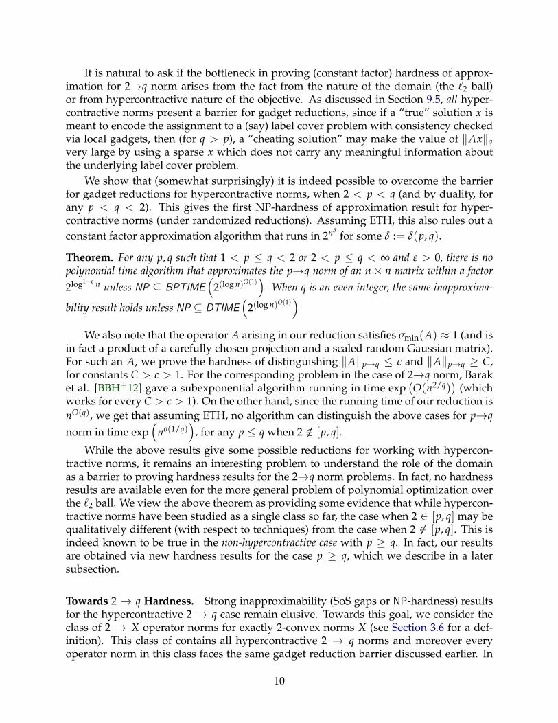
It is natural to ask if the bottleneck in proving (constant factor) hardness of approx-imation for 2→q norm arises from the fact from the nature of the domain (the `2 ball)or from hypercontractive nature of the objective. As discussed in Section 9.5, all hyper-contractive norms present a barrier for gadget reductions, since if a “true” solution x ismeant to encode the assignment to a (say) label cover problem with consistency checkedvia local gadgets, then (for q > p), a “cheating solution” may make the value of ‖Ax‖qvery large by using a sparse x which does not carry any meaningful information aboutthe underlying label cover problem.
We show that (somewhat surprisingly) it is indeed possible to overcome the barrierfor gadget reductions for hypercontractive norms, when 2 < p < q (and by duality, forany p < q < 2). This gives the first NP-hardness of approximation result for hyper-contractive norms (under randomized reductions). Assuming ETH, this also rules out aconstant factor approximation algorithm that runs in 2nδ
for some δ := δ(p, q).
Theorem. For any p, q such that 1 < p ≤ q < 2 or 2 < p ≤ q < ∞ and ε > 0, there is nopolynomial time algorithm that approximates the p→q norm of an n× n matrix within a factor2log1−ε n unless NP ⊆ BPTIME
(2(log n)O(1)
). When q is an even integer, the same inapproxima-
bility result holds unless NP ⊆ DTIME(
2(log n)O(1))
We also note that the operator A arising in our reduction satisfies σmin(A) ≈ 1 (and isin fact a product of a carefully chosen projection and a scaled random Gaussian matrix).For such an A, we prove the hardness of distinguishing ‖A‖p→q ≤ c and ‖A‖p→q ≥ C,for constants C > c > 1. For the corresponding problem in the case of 2→q norm, Baraket al. [BBH+12] gave a subexponential algorithm running in time exp
(O(n2/q)
)(which
works for every C > c > 1). On the other hand, since the running time of our reduction isnO(q), we get that assuming ETH, no algorithm can distinguish the above cases for p→qnorm in time exp
(no(1/q)
), for any p ≤ q when 2 /∈ [p, q].
While the above results give some possible reductions for working with hypercon-tractive norms, it remains an interesting problem to understand the role of the domainas a barrier to proving hardness results for the 2→q norm problems. In fact, no hardnessresults are available even for the more general problem of polynomial optimization overthe `2 ball. We view the above theorem as providing some evidence that while hypercon-tractive norms have been studied as a single class so far, the case when 2 ∈ [p, q] may bequalitatively different (with respect to techniques) from the case when 2 /∈ [p, q]. This isindeed known to be true in the non-hypercontractive case with p ≥ q. In fact, our resultsare obtained via new hardness results for the case p ≥ q, which we describe in a latersubsection.
Towards 2 → q Hardness. Strong inapproximability (SoS gaps or NP-hardness) resultsfor the hypercontractive 2 → q case remain elusive. Towards this goal, we consider theclass of 2 → X operator norms for exactly 2-convex norms X (see Section 3.6 for a def-inition). This class of contains all hypercontractive 2 → q norms and moreover everyoperator norm in this class faces the same gadget reduction barrier discussed earlier. In
10
1 2
2
∞
∞
p
q≤ minγq∗/γp∗ , γp/γq [Ste05]
≤ KG [Nes98]
≥ 1/(γqγp∗) [∗]≥ π/2 (∞→ 1) [BRS15]
≥ 2log1−ε n [∗]
≥ 2log1−ε n [BV11]
≥ 2log1−ε n [∗]
≥ 2log1−ε n [BV11]
≥ 2log1/2−ε n [BBH+12]
(Assuming ETH)
≤ 1.15/(γq γp∗) [∗]
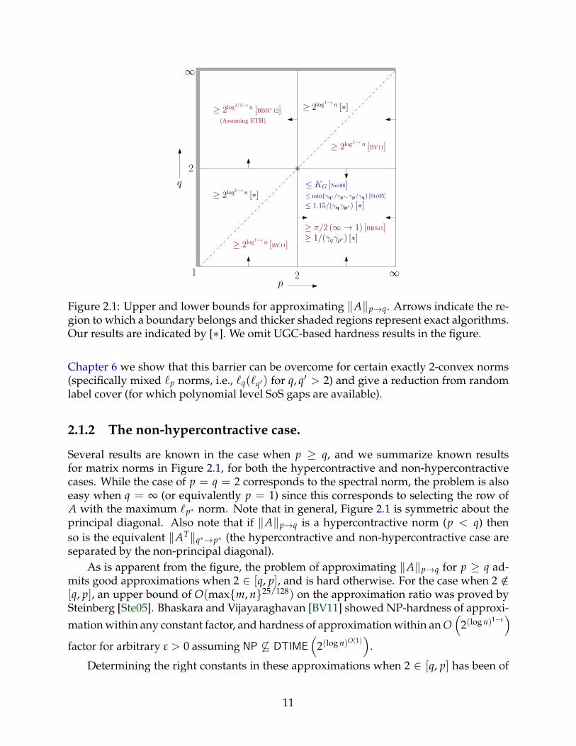
Figure 2.1: Upper and lower bounds for approximating ‖A‖p→q. Arrows indicate the re-gion to which a boundary belongs and thicker shaded regions represent exact algorithms.Our results are indicated by [∗]. We omit UGC-based hardness results in the figure.
Chapter 6 we show that this barrier can be overcome for certain exactly 2-convex norms(specifically mixed `p norms, i.e., `q(`q′) for q, q′ > 2) and give a reduction from randomlabel cover (for which polynomial level SoS gaps are available).
2.1.2 The non-hypercontractive case.
Several results are known in the case when p ≥ q, and we summarize known resultsfor matrix norms in Figure 2.1, for both the hypercontractive and non-hypercontractivecases. While the case of p = q = 2 corresponds to the spectral norm, the problem is alsoeasy when q = ∞ (or equivalently p = 1) since this corresponds to selecting the row ofA with the maximum `p∗ norm. Note that in general, Figure 2.1 is symmetric about theprincipal diagonal. Also note that if ‖A‖p→q is a hypercontractive norm (p < q) thenso is the equivalent ‖AT‖q∗→p∗ (the hypercontractive and non-hypercontractive case areseparated by the non-principal diagonal).
As is apparent from the figure, the problem of approximating ‖A‖p→q for p ≥ q ad-mits good approximations when 2 ∈ [q, p], and is hard otherwise. For the case when 2 /∈[q, p], an upper bound of O(maxm, n25/128) on the approximation ratio was proved bySteinberg [Ste05]. Bhaskara and Vijayaraghavan [BV11] showed NP-hardness of approxi-mation within any constant factor, and hardness of approximation within an O
(2(log n)1−ε
)factor for arbitrary ε > 0 assuming NP 6⊆ DTIME
(2(log n)O(1)
).
Determining the right constants in these approximations when 2 ∈ [q, p] has been of
11
considerable interest in the analysis and optimization community. For the case of ∞→1norm, Grothendieck’s theorem [Gro53] shows that the integrality gap of a semidefiniteprogramming (SDP) relaxation is bounded by a constant, and the (unknown) optimalvalue is now called the Grothendieck constant KG. Krivine [Kri77] proved an upperbound of π/(2 ln(1 +
√2)) = 1.782 . . . on KG, and it was later shown by Braverman
et al. that KG is strictly smaller than this bound. The best known lower bound on KG isabout 1.676, due to (an unpublished manuscript of) Reeds [Ree91] (see also [KO09] for aproof).
An upper bound of KG on the approximation factor also follows from the work ofNesterov [Nes98] for any p ≥ 2 ≥ q. A later work of Steinberg [Ste05] also gave anupper bound of min
γp/γq, γq∗/γp∗
, where γp denotes pth norm of a standard normal
random variable (i.e., the p-th root of the p-th Gaussian moment). Note that Steinberg’sbound is less than KG for some values of (p, q), in particular for all values of the form(2, q) with q ≤ 2 (and equivalently (p, 2) for p ≥ 2), where it equals 1/γq (and 1/γp∗ for(p, 2)).
On the hardness side, Briët, Regev and Saket [BRS15] showed NP-hardness of π/2 forthe ∞→1 norm, strengthening a hardness result of Khot and Naor based on the UniqueGames Conjecture (UGC) [KN09] (for a special case of the Grothendieck problem whenthe matrix A is positive semidefinite). Assuming UGC, a hardness result matching Reeds’lower bound was proved by Khot and O’Donnell [KO09], and hardness of approximatingwithin KG was proved by Raghavendra and Steurer [RS09].
For a related problem known as the Lp-Grothendieck problem, where the goal is tomaximize 〈x, Ax〉 for ‖x‖p ≤ 1, results by Steinberg [Ste05] and Kindler, Schechtmanand Naor [KNS10] give an upper bound of γ2
p, and a matching lower bound was provedassuming UGC by [KNS10], which was strengthened to NP-hardness by Guruswami et al.[GRSW16]. However, note that this problem is quadratic and not necessarily bilinear, andis in general much harder than the Grothendieck problems considered here. In particular,the case of p = ∞ only admits an Θ(log n) approximation instead of KG for the bilinearversion [AMMN06, ABH+05].
The Search For Optimal Constants and Optimal Rounding Algorithms. Determiningthe right approximation ratio for these problems often leads to the development of round-ing algorithms that apply much more broadly. For the Grothendieck problem, the goalis to find y ∈ Rm and x ∈ Rn with ‖y‖∞, ‖x‖∞ ≤ 1, and one considers the followingsemidefinite relaxation:
maximize ∑i,j
Ai,j · 〈ui , vj〉 s.t.
subject to ‖ui‖2 ≤ 1, ‖vj‖2 ≤ 1 ∀i ∈ [m], j ∈ [n]
ui, vj ∈ Rm+n ∀i ∈ [m], j ∈ [n]
12
By the bilinear nature of the problem above, it is clear that the optimal x, y can be takento have entries in −1, 1. A bound on the approximation ratio1 of the above program isthen obtained by designing a good “rounding” algorithm which maps the vectors ui, vj tovalues in −1, 1. Krivine’s analysis [Kri77] corresponds to a rounding algorithm whichconsiders a random vector g ∼ N (0, Im+n) and rounds to x, y defined as
yi := sgn(⟨
ϕ(ui), g⟩)
and xj := sgn(⟨
ψ(vj), g⟩)
,
for some appropriately chosen transformations ϕ and ψ. This gives the following upperbound on the approximation ratio of the above relaxation, and hence on the value of theGrothendieck constant KG:
KG ≤1
sinh−1(1)· π
2=
1ln(1 +
√2)· π
2.
Braverman et al. [BMMN13] show that the above bound can be strictly improved (by avery small amount) using a two dimensional analogue of the above algorithm, where thevalue yi is taken to be a function of the two dimensional projection (〈ϕ(ui), g1〉, 〈ϕ(ui), g2〉)for independent Gaussian vectors g1, g2 ∈ Rm+n (and similarly for x). Naor and Regev[NR14] show that such schemes are optimal in the sense that it is possible to achievean approximation ratio arbitrarily close to the true (but unknown) value of KG by usingk-dimensional projections for a large (constant) k. A similar existential result was alsoproved by Raghavendra and Steurer [RS09] who proved that the there exists a (slightlydifferent) rounding algorithm which can achieve the (unknown) approximation ratio KG.
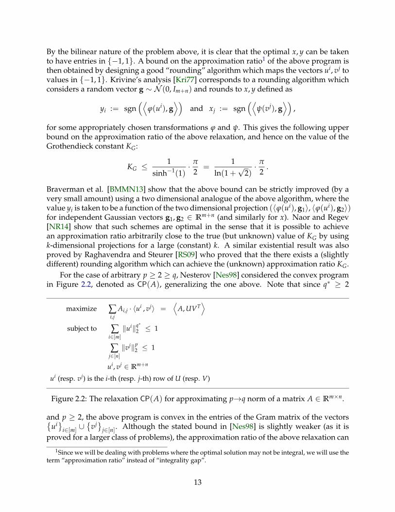
For the case of arbitrary p ≥ 2 ≥ q, Nesterov [Nes98] considered the convex programin Figure 2.2, denoted as CP(A), generalizing the one above. Note that since q∗ ≥ 2
maximize ∑i,j
Ai,j · 〈ui , vj〉 =⟨
A, UVT⟩
subject to ∑i∈[m]
‖ui‖q∗2 ≤ 1
∑j∈[n]‖vj‖p
2 ≤ 1
ui, vj ∈ Rm+n
ui (resp. vj) is the i-th (resp. j-th) row of U (resp. V)
Figure 2.2: The relaxation CP(A) for approximating p→q norm of a matrix A ∈ Rm×n.
and p ≥ 2, the above program is convex in the entries of the Gram matrix of the vectorsui
i∈[m] ∪
vjj∈[n]. Although the stated bound in [Nes98] is slightly weaker (as it is
proved for a larger class of problems), the approximation ratio of the above relaxation can
1Since we will be dealing with problems where the optimal solution may not be integral, we will use theterm “approximation ratio” instead of “integrality gap”.
13
Out[220]=
5 10 15 20 25p
1.5
2.0
2.5
3.0
3.5
Apx Factor
Krivine
Steinberg
ThisPaper
Printed by Wolfram Mathematica Student Edition
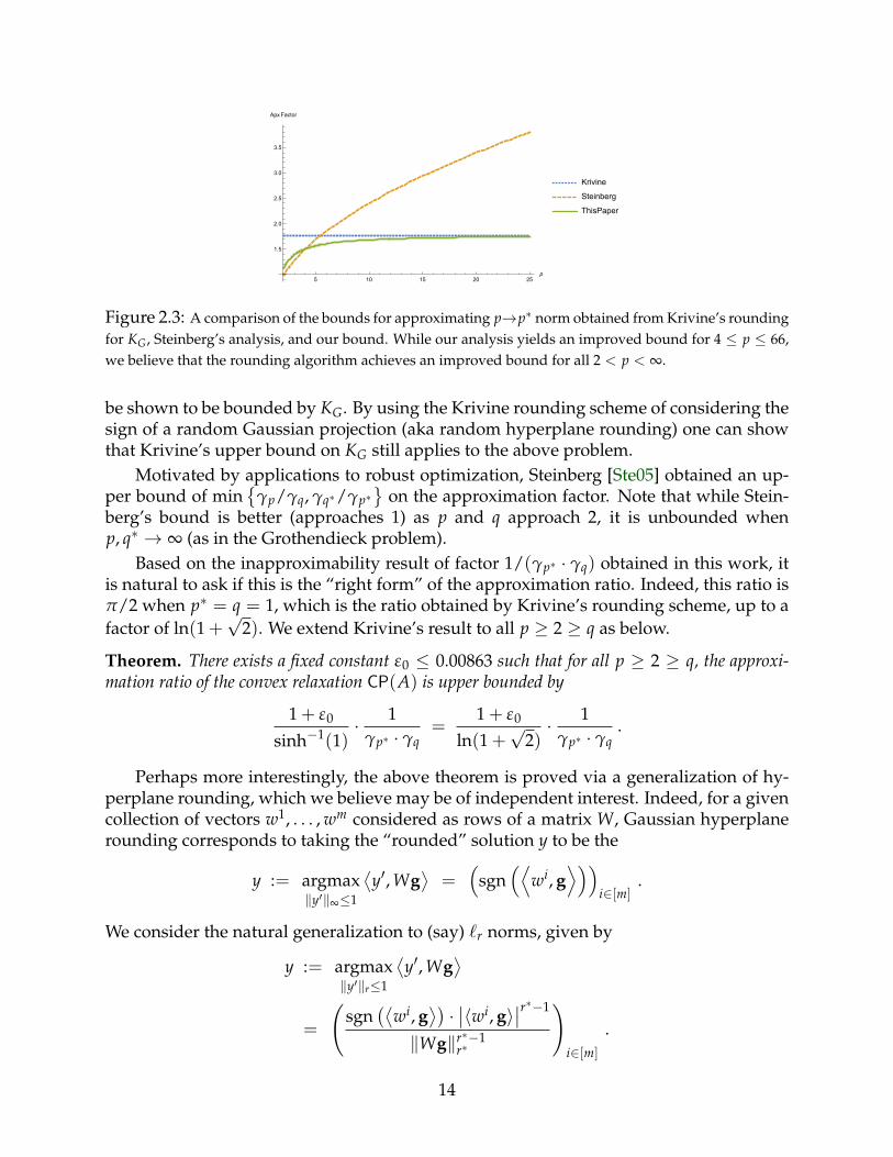
Figure 2.3: A comparison of the bounds for approximating p→p∗ norm obtained from Krivine’s roundingfor KG, Steinberg’s analysis, and our bound. While our analysis yields an improved bound for 4 ≤ p ≤ 66,we believe that the rounding algorithm achieves an improved bound for all 2 < p < ∞.
be shown to be bounded by KG. By using the Krivine rounding scheme of considering thesign of a random Gaussian projection (aka random hyperplane rounding) one can showthat Krivine’s upper bound on KG still applies to the above problem.
Motivated by applications to robust optimization, Steinberg [Ste05] obtained an up-per bound of min
γp/γq, γq∗/γp∗
on the approximation factor. Note that while Stein-
berg’s bound is better (approaches 1) as p and q approach 2, it is unbounded whenp, q∗ → ∞ (as in the Grothendieck problem).
Based on the inapproximability result of factor 1/(γp∗ · γq) obtained in this work, itis natural to ask if this is the “right form” of the approximation ratio. Indeed, this ratio isπ/2 when p∗ = q = 1, which is the ratio obtained by Krivine’s rounding scheme, up to afactor of ln(1 +
√2). We extend Krivine’s result to all p ≥ 2 ≥ q as below.
Theorem. There exists a fixed constant ε0 ≤ 0.00863 such that for all p ≥ 2 ≥ q, the approxi-mation ratio of the convex relaxation CP(A) is upper bounded by
1 + ε0
sinh−1(1)· 1
γp∗ · γq=
1 + ε0
ln(1 +√
2)· 1
γp∗ · γq.
Perhaps more interestingly, the above theorem is proved via a generalization of hy-perplane rounding, which we believe may be of independent interest. Indeed, for a givencollection of vectors w1, . . . , wm considered as rows of a matrix W, Gaussian hyperplanerounding corresponds to taking the “rounded” solution y to be the
y := argmax‖y′‖∞≤1
⟨y′, Wg
⟩=(
sgn(⟨
wi, g⟩))
i∈[m].
We consider the natural generalization to (say) `r norms, given by
y := argmax‖y′‖r≤1
⟨y′, Wg
⟩=
(sgn
(⟨wi, g
⟩)·∣∣〈wi, g〉
∣∣r∗−1
‖Wg‖r∗−1r∗
)i∈[m]
.
14
We refer to y as the “Hölder dual” of Wg, since the above rounding can be obtained byviewing Wg as lying in the dual (`r∗) ball, and finding the y for which Hölder’s inequalityis tight. Indeed, in the above language, Nesterov’s rounding corresponds to consideringthe `∞ ball (hyperplane rounding). While Steinberg used a somewhat different relaxation,the rounding there can be obtained by viewing Wg as lying in the primal (`r) ball insteadof the dual one. In case of hyperplane rounding, the analysis is motivated by the identitythat for two unit vectors u and v, we have
Eg[sgn(〈g, u〉) · sgn(〈g, v〉)] =
2π· sin−1(〈u, v〉) .
We prove the appropriate extension of this identity to `r balls (and analyze the functionsarising there) which may also be of interest for other optimization problems over `r balls.
Hardness. We extend the hardness results of [BRS15] for the ∞ → 1 and 2 → 1 normsof a matrix to any p ≥ 2 ≥ q. The hardness factors obtained match the performanceof known algorithms (due to Steinberg [Ste05]) for the cases of 2 → q and p → 2, andmoreover almost match the algorithmic results in the more general case of p ≥ 2 ≥ q.
Theorem. For any p, q such that p ≥ 2 ≥ q and ε > 0, it is NP-hard to approximate the p→qnorm within a factor 1/(γp∗γq)− ε.
2.2 Polynomial Optimization over the Sphere
In Chapter 8 and Chapter 9 we study the problem of optimizing homogeneous polynomi-als over the unit sphere. Formally, given an n-variate degree-d homogeneous polynomialf , the goal is to compute ‖ f ‖2 := sup‖x‖2=1 | f (x)|. For d ≥ 3, it defines a natural higher-order analogue of the eigenvalue problem for matrices. The problem also provides animportant testing ground for the development of new spectral and semidefinite program-ming (SDP) techniques, and techniques developed in the context of this problem have hadapplications to various other constrained settings [HLZ10, Lau09, Las09]. Besides beinga natural and fundamental problem in its own right, it has connections to widely studiedquestions in many other areas, like the small set expansion hypothesis [BBH+12, BKS14],tensor low-rank decomposition and tensor PCA [BKS15, GM15, MR14, HSS15], refutationof random constraint satisfaction problems [RRS16] and planted clique [BV09].
Optimization over Sn−1 has been given much attention in the optimization commu-nity, where for a fixed number of variables n and degree d of the polynomial, it is knownthat the estimates produced by q levels a certain hierarchy of SDPs (Sum of Squares) getarbitrarily close to the true optimal solution as q increases (see [Las09] for various ap-plications). We refer the reader [dKL19, DW12, Fay04, dKLS14] for more information onconvergence results. These algorithms run in time nO(q), which is polynomial for con-stant q. Unfortunately, known convergence results often give sub-optimal bounds whenq is sub-linear in n.
15
In computer science, much attention has been given to the sub-exponential runtimeregime (i.e. q n) since many of the target applications such as SSE, QMA and refut-ing random CSPs are of considerable interest in this regime. In addition to the polytimend/2−1-approximation for general polynomials [HLZ10, So11], approximation guaranteeshave been proved for several special cases including 2 → q norms [BBH+12], polynomi-als with non-negative coefficients [BKS14], and some polynomials that arise in quantuminformation theory [BKS17, BH13]. An outstanding open problem in quantum informa-tion theory is settling the complexity of the best separable state problem (which can beviewed as seeking a (1 + ε)-approximation for maximizing a certain class of polynomialsover the sphere), and the sum of squares (SoS) hierarchy captures all known algorithmsfor this problem upto a logarithm in the exponent [BKS14, BKS17]. The best known up-per bound being
√n levels due to Barak, Kothari and Steurer [BKS17] and the best lower
bound being log n levels due to Harrow, Natarajan and Wu [HNW16]. Hence there isconsiderable interest in understanding the approximation/runtime tradeoff (especiallyin the sub-exponential regime).
In this thesis, we develop general techniques to design and analyze algorithms forpolynomial optimization over the sphere. The sphere constraint is one of the simplestconstraints for polynomial optimization and thus is a good testbed for techniques. In-deed, we believe these techniques will also be useful in understanding polynomial opti-mization for other constrained settings.
In addition to giving an analysis the problem for arbitrary polynomials, these tech-niques can also be adapted to take advantage of the structure of the input polynomial,yielding better approximations for several special cases such as polynomials with non-negative coefficients, and sparse polynomials. Previous polynomial time algorithms forpolynomial optimization work by reducing the problem to diameter estimation in convexbodies [So11] and seem unable to utilize structural information about the (class of) inputpolynomials. Development of a method which can use such information was stated as anopen problem by Khot and Naor [KN08] (in the context of `∞ optimization).
Our approximation guarantees are with respect to the optimum at each level of theSoS hierarchy. Such SDPs are the most natural tools to bound the optima of polynomialoptimization problems, and our results shed light on the efficacy of higher levels of theSoS hierarchy to deliver better approximations to the optimum.
- In Chapter 8 we introduce a technique we refer to as “weak decoupling inequalities”and use it to upper-bound the integrality gap of q levels of the SoS hierarchy for variousclasses of polynomials over the sphere, namely arbitrary polynomials (when q n, ourresult yields better bounds than those implied by convergence results [DW12, dKL19]2),polynomials with non-negative coefficients and sparse polynomials:
Aribitrary. SoSq gets an (O(n)/q)d/2−1 approximation.
Non-negative Coefficients. SoSq gets an (O(n)/q)d/4−1/2 approximation.
Sparse. SoSq gets a√
m/q approximation where m is the sparsity.
2[dKL19] appeared after the publication of this work
16
We believe that these techniques are applicable to much broader settings.
- In Chapter 8 we also prove for a certain hierarchy of relaxations for optimization overthe sphere that “robust” integrality gaps for lower levels of the hierarchy can be lifted tointegrality gaps for higher levels. This hierarchy is closely related to the SoS hierarchybut is possibly weaker (in fact a majority of the works studying SoS and optimizationover the sphere can be seen as using only this weaker hierarchy). We give an exam-ple application of this result by using it to show polynomial level integrality gaps (forthe aforementioned weaker hierarchy of relaxations) for optimizing non-negative coef-ficient polynomials.3 We hope that this method can find applications in other settingsand perhaps even be shown to work in the context of the SoS hierarchy.
- In Chapter 9, we show an upper bound on the integrality gap of q levels of SoS onpolynomials with random coefficients4. Specifically we show that SoS certifies an up-per bound that is an (O(n)/q)d/4−1/2 approximation to the true value. An interestingconsequence of our result is that random/spiked-random instances cannot provide BestSeparable State gap instances for more than polylog levels of SoS.
3 Integrality gaps for polynomial levels of SoS are already known in the case of arbitrary polynomialsdue to a result of Hopkins et al. [HKP+17]. More precisely, they show polynomial level integrality gaps forpolynomials with i.i.d. ±1 random coefficients.
4[RRS16] concurrently obtained slightly weaker bounds. However their bounds apply for the moregeneral model of sparse random polynomials thereby finding applications to refutation of random CSPs.
17
Part II
Degree-2 (Operator Norms)
18
Chapter 3
Preliminaries (Normed Spaces)
3.1 Vectors
Unless otherwise specified, vectors are assumed to be finite dimensional with real valuedcoordinates. For a vector x ∈ Rn, we denote its i-th coordinate by xi (Chapter 5 is the onlyexception to this wherein it is more convenient to think of vectors as functions and so thenotation x(i) is used).We denote sequences of vectors with superscripts, e.g. x1, x2, · · · ∈ Rn.For x, y ∈ Rn we let 〈x , y〉 denote the inner product under the counting measure, i.e.,
〈x , y〉 := ∑i∈[n]
xi · yi
For a scalar function f : R → R and x ∈ Rn we denote by f [x] ∈ Rn the vector obtainedby applying f to x entry-wise.For a vector u, we use Du to denote the diagonal matrix with the entries of u forming thediagonal, and for a matrix M we use diag(M) to denote the vector of diagonal entries.
3.2 Norms
A function ‖·‖X from Rn to the non-negative reals is called a norm if it satisfies
Subadditivity. ‖x + y‖X ≤ ‖x‖X + ‖y‖X.
Absolute Homogeneity. ‖c · x‖X = |c| · ‖x‖X for any c ∈ R.
Positive Definiteness. ‖x‖X = 0 implies x = 0.
We say a convex body K is symmetric if K = −K (i.e., x ∈ K ⇒ −x ∈ K). There isa well known correspondence between norms and symmetric convex bodies. The mapfrom norms to symmetric convex bodies is referred to as the unit ball of the norm and isdefined as
Ball(X) := x | ‖x‖X ≤ 1.
19
The inverse map is known as the Minkowski functional and is defined as
‖x‖ := inft>0x/t ∈ K.
The dual space of Rn is Rn itself. For a norm X and ξ ∈ Rn, the dual norm is defined as
‖ξ‖X∗ := supx∈Ball(X)
〈ξ , x〉
We will often consider families of normed spaces of increasing dimension, and we willdenote this by (Xn)n∈N where Xn is assumed to be a norm over Rn.
3.3 `p Norms
For p ≥ 1 and a vector x, we denote the counting `p-norm as ‖x‖p := (∑i |xi|p)1/p (whenp = ∞ it is defined as maxi∈[n] |xi|).For any p ∈ [1, ∞], the dual norm of `p is `p∗ , where p∗ is defined as satisfying the equality:1p +
1p∗ = 1. Formally,
Fact 3.3.1. For any p ∈ [1, ∞], ‖ξ‖p∗ = supx∈Ball(`p)〈ξ , x〉.
For p ≥ 1, we define the p-th Gaussian norm of a standard gaussian g as
γp := ( Eg∼N (0,1)
[|g|p
])
1/p .
3.4 Operator Norm
For a linear operator A mapping a normed space X over Rn to normed space Y over Rm,the operator norm is defined as the maximum amount that A stretches an X-unit vectorwhere stretch is measured according to Y i.e.,
‖A‖X→Y := maxx∈Rn\0
‖Ax‖Y/‖x‖X
We say two normed spaces X, Y are isomorphic (resp. isometric) to one another if there ex-ists an invertible linear operator A : X → Y such that A and A−1 have bounded operatornorm (resp. operator norm 1).1 In the case where X = `p, Y = `q, we’ll use the shorthand‖A‖p→q to denote the operator norm.We next record the equivalence of operator norms with bilinear form maximization.
1 Since any two norms over a finite dimensional space are isomorphic, this notion is only interesting ininfinite dimensional settings. The notion of isometry however remains interesting in the finite dimensionalsetting.
20
Fact 3.4.1. For any linear operator A : X → Y,
‖A‖X→Y = sup‖y‖Y∗≤1
sup‖x‖X≤1
〈y , Ax〉 = ‖AT‖Y∗→X∗ .
Proof. Using the fact that 〈y , Ax〉 = 〈x , ATy〉,
‖A‖X→Y = sup‖x‖X≤1
‖Ax‖Y = sup‖x‖X≤1
sup‖y‖Y∗≤1
〈y , Ax〉 = sup‖x‖X≤1
sup‖y‖Y∗≤1
〈x , ATy〉
= sup‖y‖Y∗≤1
‖ATy‖X∗ = ‖AT‖Y∗→X∗ .
Operator norms are submultiplicative in the following sense:
Fact 3.4.2. For any norms X, Y, Z, and linear operators C : X → Y, B : Y → Z,
‖BC‖X→Z = supx
‖BCx‖Z
‖x‖X≤ sup
x
‖B‖Y→Z‖Cx‖Y
‖x‖X= ‖C‖X→Y‖B‖Y→Z.
3.5 Type and Cotype
The notions of Type and Cotype are powerful classification tools from Banach space the-ory.
Definition 3.5.1. The Type-2 constant of a Banach space X, denoted by T2(X), is the smallestconstant C such that for every finite sequence of vectors xi in X,
E
[‖∑
iεi · xi‖
]≤ C ·
√∑
i‖xi‖2
where εi is an independent Rademacher random variable. We say X is of Type-2 if T2(X) < ∞.2
Definition 3.5.2. The Cotype-2 constant of a Banach space X, denoted by C2(X), is the smallestconstant C such that for every finite sequence of vectors xi in X,
E
[‖∑
iεi · xi‖
]≥ 1
C·√
∑i‖xi‖2
where εi is an independent Rademacher random variable. We say X is of Cotype-2 if C2(X) < ∞.
Remark 3.5.3.2 T2(X) < ∞ is yet another property that is uninteresting in the finite dimensional setting since every
finite dimensional norm is of Type-2 by John’s theorem. However for a sequence of norms (Xn)n∈N, thedependence of T2(Xn) on the dimension n is an interesting and useful property to track and statementsderived from Type-2 properties of infinite dimensional spaces can often be adapted to give quantitativefinite dimensional versions when considering a sequence of norms of growing dimension.
21
- It is known that C2(X∗) ≤ T2(X).
- It is known that for p ≥ 2, we have T2(`np) = γp (while C2(`
np) → ∞ as n → ∞) and for
q ≤ 2, C2(`nq ) = max21/q−1/2, 1/γq (while T2(`
nq )→ ∞ as n→ ∞).
We say X is Type-2 (resp. Cotype-2) if T2(X) < ∞ (resp. C2(X) < ∞). T2(X) and C2(X)can be regarded as measures of the “closeness” of X to a Hilbert space. Some notablemanifestations of this correspondence are:
- T2(X) = C2(X) = 1 if and only if X is isometric to a Hilbert space.
- Kwapien [Kwa72a]: X is of Type-2 and Cotype-2 if and only if it is isomorphic to aHilbert space.
- Figiel, Lindenstrauss and Milman [FLM77]: If X is a Banach space of Cotype-2,then any n-dimensional subspace of X has an m = Ω(n)-dimensional subspacewith Banach-Mazur distance at most 2 from `m
2 .
More generally one defines
Definition 3.5.4 (Type/Cotype). For 1 ≤ p ≤ 2, the Type-p constant of a normed space X,denoted by Tp(X), is the smallest constant C such that for every finite sequence of vectors xi inX,
E
[‖∑
iεi · xi‖
]≤ C ·
(∑
i‖xi‖p
)1/p
where εi is an independent Rademacher random variable. X is said to have Type-p if Tp(X) < ∞.
For 2 ≤ q ≤ ∞, the Cotype-q constant of a normed space X, denoted by Cq(X), is the smallestconstant C such that for every finite sequence of vectors xi in X,
E
[‖∑
iεi · xi‖
]≥ 1
C·(
∑i‖xi‖q
)1/q
.
X is said to have Cotype-q if Cq(X) < ∞.
Any normed space X trivially is Type-1 and Cotype-∞. It is easily checked that Type-p implies Type-p′ for any p′ ≤ p and Cotype-q implies Cotype-q′ for any q ≥ q′. LetpX := supp | Tp(X) < ∞ and qX := infq | Cq(X) < ∞. pX (resp. qX) is referred to asthe modulus of Type (resp. Cotype).Another example of the power of these notions in classifying Banach spaces is the cele-brated MP+K theorem:
Theorem 3.5.5 (Maurey and Pisier + Krivine). Any infinite dimensional Banach space X con-tains for any ε > 0, (1 + ε)-isomorphs of `pX and `qX of arbitrarily large dimension.
22
3.6 p-convexity and q-concavity
The notions of p-convexity and q-concavity are well defined for a wide class of normedspaces known as Banach lattices. In this document we only define these notions for finitedimensional norms that are 1-unconditional in the elementary basis (i.e., those norms Xfor which flipping the sign of an entry of x does not change the norm. We shall refer tosuch norms as sign-invariant norms). Most of the statements we make in this context canbe readily extended to the case of norms admitting some 1-unconditional basis, but wechoose to fix the elementary basis in the interest of clarity. With respect to the goals ofthis document, we believe most of the key insights are already manifest in the elementarybasis case.
Definition 3.6.1 (p-convexity/q-concavity). Let X be a sign-invariant norm over Rn. Thenfor 1 ≤ p ≤ ∞ the p-convexity constant of X, denoted by M(p)(X), is the smallest constant Csuch that for every finite sequence of vectors xi in X,∥∥∥∥∥∥
[∑
i|[xi]|p
]1/p∥∥∥∥∥∥ ≤ C ·
(∑
i‖xi‖p
)1/p
X is said to be p-convex if M(p)(X) < ∞. We will say X is exactly p-convex if M(p)(X) = 1.
For 1 ≤ q ≤ ∞, the q-concavity constant of X, denoted by M(q)(X), is the smallest constant Csuch that for every finite sequence of vectors xi in X,∥∥∥∥∥∥
[∑
i|[xi]|q
]1/q∥∥∥∥∥∥ ≥ 1
C·(
∑i‖xi‖q
)1/q
.
X is said to be q-concave if M(q)(X) < ∞.We will say X is exactly q-concave if M(q)(X) = 1.
Every sign-invariant norm is exactly 1-convex and ∞-concave.
For a sign-invariant norm X over Rn, and any 0 < p < ∞ let X(p) denote the function‖|[x]|p‖1/p
X . X(p) is referred to as the p-convexification of X. It is easily verified thatM(p)(X(p)) = M(1)(X) and further that X(p) is an exactly p-convex sign-invariant normif and only if X is a sign-invariant norm (and therefore exactly 1-convex).
3.7 Convex Relaxation for Operator Norm
In this section we will see that there is a natural convex relaxation for a wide class of op-erator norms. It is instructive to first consider the pertinent relaxation for Grothendieck’sinequality. Recall the bilinear formulation of the problem wherein given an m× n matrix
23
A, the goal is to maximize yT A x over ‖y‖∞, ‖x‖∞ ≤ 1. One then considers the followingsemidefinite programming relaxation:
maximize ∑i,j
Ai,j · 〈ui , vj〉 s.t.
subject to ‖ui‖2 ≤ 1, ‖vj‖2 ≤ 1 ∀i ∈ [m], j ∈ [n]
ui, vj ∈ Rm+n ∀i ∈ [m], j ∈ [n]
which is equivalent to
maximize12·⟨[
0 AAT 0
],[
Y W
WT X
]⟩s.t.
Xi,i ≤ 1, Yj,j ≤ 1[Y W
WT X
] 0, Y ∈ Sm×m, X ∈ Sn×n, W ∈ Rm×n
where Sm×m is the set of m×m symmetric positive semidefinite matrices in Rm×m.
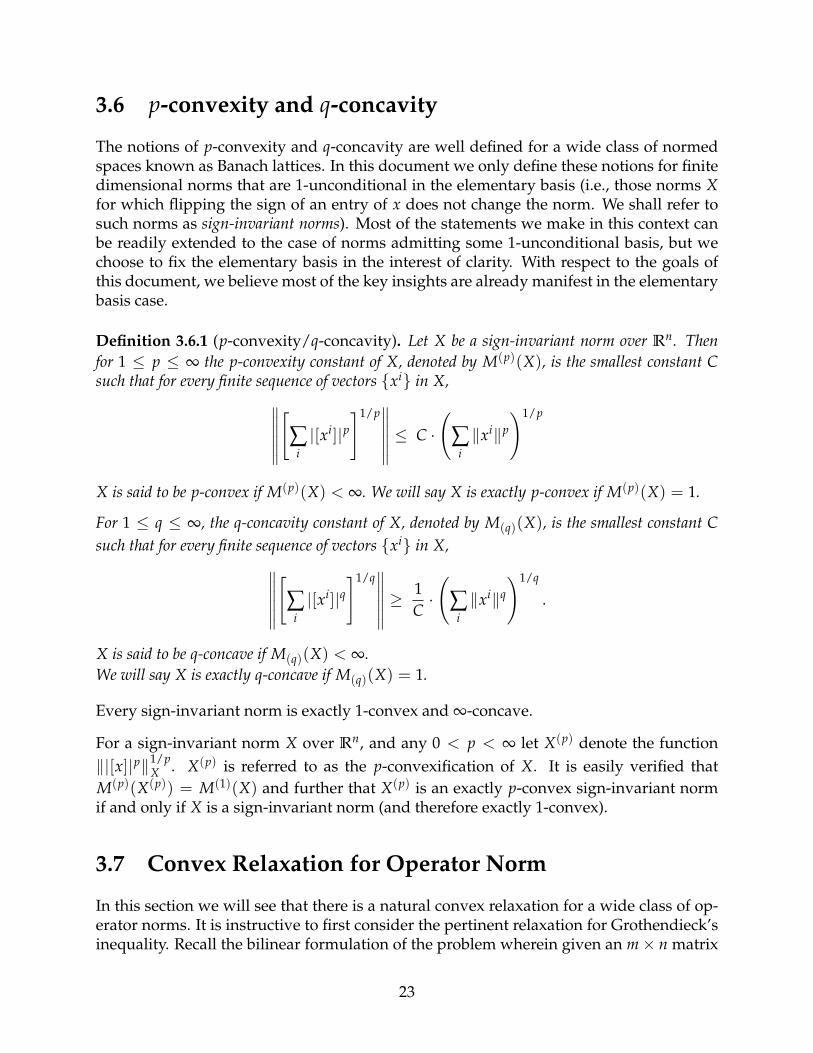
Nesterov [Nes98, NWY00]3 and independently Naor and Schechtman4 observed that if Xand Y∗ are exactly 2-convex, then there is a natural computable convex relaxation for thebilinear formulation of X → Y operator norm. Recall the goal is to maximize yT A x over‖y‖Y∗ , ‖x‖X ≤ 1. The relaxation which we will call CP(A) is as follows:
maximize12·⟨[
0 AAT 0
],[
Y W
WT X
]⟩s.t.
diag(X) ∈ Ball(X(1/2)), diag(Y) ∈ Ball(Y∗(1/2))[Y W
WT X
] 0, Y ∈ Sm×m, X ∈ Sn×n, W ∈ Rm×n
For a vector s, let Ds denote the diagonal matrix with s as diagonal entries. Let X :=(X(1/2))∗, Y := (Y∗(1/2))∗. We can then define the dual program DP(A) as follows:
minimize (‖s‖Y + ‖t‖X)/2 s.t.[Ds −A−AT Dt
] 0, s ∈ Rm, t ∈ Rn .
Strong duality is satisfied, i.e. DP(A) = CP(A), and a proof can be found in [NWY00](see Lemma 13.2.2 and Theorem 13.2.3).
3 Nesterov uses the language of quadratic programming and appears not to have noticed the connectionsto Banach space theory. In fact, it appears that Nesterov even gave yet another proof of an O(1) upperbound on Grothendieck’s constant.
4personal communication
24
3.8 Factorization of Linear Operators
Let X, Y, E be Banach spaces and let A : X → Y be a continuous linear operator. We saythat A factorizes through E if there exist continuous operators C : X → E and B : E → Ysuch that A = BC. Factorization theory has been a major topic of study in functionalanalysis, going as far back as Grothendieck’s famous “Resume” [Gro53]. It has manystriking applications, like the isomorphic characterization of Hilbert spaces and Lp spacesdue to Kwapien [Kwa72a, Kwa72b], connections to type and cotype through the work ofKwapien [Kwa72a], Rosenthal [Ros73], Maurey [Mau74] and Pisier [Pis80], connectionsto Sidon sets through the work of Pisier [Pis86], characterization of weakly compact op-erators due to Davis et al. [DFJP74], connections to the theory of p-summing operatorsthrough the work of Grothendieck [Gro53], Pietsch [Pie67] and Lindenstrauss and Pel-czynski [LP68].
Let Φ(A) denote
Φ(A) := infH
infBC=A
‖C‖X→H · ‖B‖H→Y
‖A‖X→Y
where the infimum runs over all Hilbert spaces H. We say A factorizes through a Hilbertspace if Φ(A) < ∞. Further, let
Φ(X, Y) := supA
Φ(A)
where the supremum runs over continuous operators A : X → Y. As a quick example ofthe power of factorization theorems, observe that if I : X → X is the identity operator on aBanach space X and Φ(I) < ∞, then X is isomorphic to a Hilbert space and moreover thedistortion (Banach-Mazur distance) is at most Φ(I) (i.e., there exists an invertible operatorT : X → H for some Hilbert space H such that ‖T‖X→H · ‖T−1‖H→X ≤ Φ(I)). In fact (asobserved by Maurey), Kwapien gave an isomorphic characterization of Hilbert spacesby proving a factorization theorem. Maurey observed that a more general factorizationresult underlies Kwapien’s work:
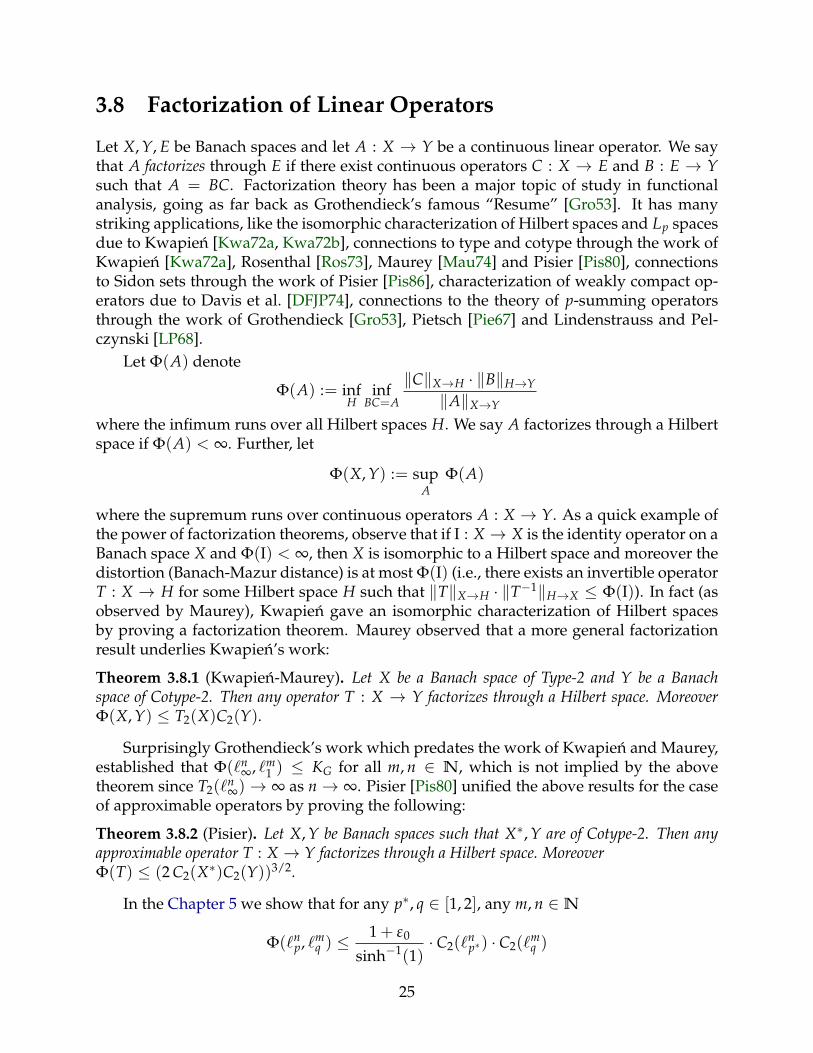
Theorem 3.8.1 (Kwapien-Maurey). Let X be a Banach space of Type-2 and Y be a Banachspace of Cotype-2. Then any operator T : X → Y factorizes through a Hilbert space. MoreoverΦ(X, Y) ≤ T2(X)C2(Y).
Surprisingly Grothendieck’s work which predates the work of Kwapien and Maurey,established that Φ(`n
∞, `m1 ) ≤ KG for all m, n ∈ N, which is not implied by the above
theorem since T2(`n∞)→ ∞ as n→ ∞. Pisier [Pis80] unified the above results for the case
of approximable operators by proving the following:
Theorem 3.8.2 (Pisier). Let X, Y be Banach spaces such that X∗, Y are of Cotype-2. Then anyapproximable operator T : X → Y factorizes through a Hilbert space. MoreoverΦ(T) ≤ (2 C2(X∗)C2(Y))3/2.
In the Chapter 5 we show that for any p∗, q ∈ [1, 2], any m, n ∈N
Φ(`np, `m
q ) ≤1 + ε0
sinh−1(1)· C2(`
np∗) · C2(`
mq )
25

which improves upon Pisier’s bound and for certain ranges of (p, q), improves upon KGas well as the bound of Kwapien-Maurey.
26
Chapter 4
Hardness results for p→q norm
In this chapter we prove NP-hardness results for approximating hypercontractive norms(i.e., p→q norm when p ≤ q). We show
Theorem 4.0.1. For any p, q such that 1 < p ≤ q < 2 or 2 < p ≤ q < ∞ and a constantc > 1, unless NP ∈ BPP, no polytime algorithm approximates p→q norm within a factor of c.The reduction runs in time nBpq for 2 < p < q, where Bp = poly(1/(1− γp∗)).
We show that the above hardness can be strengthened to any constant factor via asimple tensoring argument. In fact, this also shows that it is hard to approximate ‖A‖p→qwithin almost polynomial factors unless NP is in randomized quasi-polynomial time.This is the content of the following theorem.
Theorem 4.0.2. For any p, q such that 1 < p ≤ q < 2 or 2 < p ≤ q < ∞ and ε > 0, there is nopolynomial time algorithm that approximates the p→q norm of an n× n matrix within a factor2log1−ε n unless NP ⊆ BPTIME
(2(log n)O(1)
). When q is an even integer, the same inapproxima-
bility result holds unless NP ⊆ DTIME(
2(log n)O(1))
En route to the above result, we also prove new results for the case when p ≥ q with2 ∈ [q, p]:
Theorem 4.0.3. For any p, q such that p ≥ 2 ≥ q and ε > 0, it is NP-hard to approximate thep→q norm within a factor 1/(γp∗γq)− ε.
where γr denotes the rth norm of a standard normal random variable, and p∗ := p/(p− 1)is the dual norm of p.
Both Theorem 4.0.1 and Theorem 4.0.3 are consequences of a more technical theorem,which proves hardness of approximating ‖A‖2→r for r < 2 (and hence ‖A‖r∗→2 for r∗ >2) while providing additional structure in the matrix A produced by the reduction. Wealso show our methods can be used to provide a simple proof (albeit via randomizedreductions) of the 2Ω((log n)1−ε) hardness for the non-hypercontractive case when 2 /∈ [q, p],which was proved by [BV11].
See Fig. 2.1 for a pictorial summary of the hardness and algorithmic results in variousregimes.
27
4.1 Proof Overview
The hardness of proving hardness for hypercontractive norms. Reductions for variousgeometric problems use a “smooth” version of the Label Cover problem, composed withlong-code functions for the labels of the variables. In various reductions, including theones by Guruswami et al. [GRSW16] and Briët et al. [BRS15] (which we closely follow)the solution vector x to the geometric problem consists of the Fourier coefficients of thevarious long-code functions, with a “block” xv for each vertex of the label-cover instance.The relevant geometric operation (transformation by the matrix A in our case) consists ofprojecting to a space which enforces the consistency constraints derived from the label-cover problem, on the Fourier coefficients of the encodings.
However, this strategy presents with two problems when designing reductions forhypercontractive norms. Firstly, while projections maintain the `2 norm of encodings cor-responding to consistent labelings and reduce that of inconsistent ones, their behaviouris harder to analyze for `p norms for p 6= 2. Secondly, the global objective of maximiz-ing ‖Ax‖q is required to enforce different behavior within the blocks xv, than in the fullvector x. The block vectors xv in the solution corresponding to a satisfying assignment oflabel cover are intended to be highly sparse, since they correspond to “dictator functions”which have only one non-zero Fourier coefficient. This can be enforced in a test using thefact that for a vector xv ∈ Rt, ‖xv‖q is a convex function of ‖xv‖p when p ≤ q, and ismaximized for vectors with all the mass concentrated in a single coordinate. However,a global objective function which tries to maximize ∑v‖xv‖q
q, also achieves a high valuefrom global vectors x which concentrate all the mass on coordinates corresponding to fewvertices of the label cover instance, and do not carry any meaningful information aboutassignments to the underlying label cover problem.
Since we can only check for a global objective which is the `q norm of some vectorinvolving coordinates from blocks across the entire instance, it is not clear how to enforcelocal Fourier concentration (dictator functions for individual long codes) and global well-distribution (meaningful information regarding assignments of most vertices) using thesame objective function. While the projector A also enforces a linear relation between theblock vectors xu and xv for all edges (u, v) in the label cover instance, using this to ensurewell-distribution across blocks seems to require a very high density of constraints in thelabel cover instance, and no hardness results are available in this regime.
Our reduction. We show that when 2 /∈ [p, q], it is possible to bypass the above issuesusing hardness of ‖A‖2→r as an intermediate (for r < 2). Note that since ‖z‖r is a concavefunction of ‖z‖2 in this case, the test favors vectors in which the mass is well-distributedand thus solves the second issue. For this, we use local tests based on the Berry-Esséentheorem (as in [GRSW16] and [BRS15]). Also, since the starting point now is the `2 norm,the effect of projections is easier to analyze. This reduction is discussed in Section 4.3.
By duality, we can interpret the above as a hardness result for ‖A‖p→2 when p > 2(using r = p∗). We then convert this to a hardness result for p→q norm in the hyper-contractive case by composing A with an “approximate isometry” B from `2 → `q (i.e.,∀y ‖By‖q ≈ ‖y‖2) since we can replace ‖Ax‖2 with ‖BAx‖q. Milman’s version of the
28
Dvoretzky theorem [Ver17] implies random operators to a sufficiently high dimensional(nO(q)) space satisfy this property, which then yields constant factor hardness results forthe p→q norm.
We also show that the hardness for hypercontractive norms can be amplified via ten-soring. This was known previously for the 2→4 norm using an argument based on par-allel repetition for QMA [HM13], and for the case of p = q [BV11]. We give a simpleargument based on convexity, which proves this for all p ≤ q, but appears to have goneunnoticed previously. The amplification is then used to prove hardness of approximationwithin almost polynomial factors.
Non-hypercontractive norms. We also use the hardness of ‖A‖2→r to obtain hardnessfor the non-hypercontractive case of ‖A‖p→q with q < 2 < p, by using an operator that“factorizes” through `2. In particular, we obtain hardness results for ‖A‖p→2 and ‖A‖2→q(of factors 1/γp∗and 1/γq respectively) using the reduction in Section 4.3. We then com-bine these hardness results using additional properties of the operator A obtained in thereduction, to obtain a hardness of factor (1/γp∗) · (1/γq) for the p→q norm for p > 2 > q.The composition, as well as the hardness results for hypercontractive norms, are pre-sented in Section 4.4.
We also obtain a simple proof of the 2Ω((log n)1−ε) hardness for the non-hypercontractivecase when 2 /∈ [q, p] (already proved by Bhaskara and Vijayaraghavan [BV11]) via anapproximate isometry argument as used in the hypercontractive case. In the hypercon-tractive case, we started from a constant factor hardness of the p→2 norm and the samefactor for p→q norm using the fact that for a random Gaussian matrix B of appropriatedimensions, we have ‖Bx‖q ≈ ‖x‖2 for all x. We then amplify the hardness via tensoring.In the non-hypercontractive case, we start with a hardness for p→p norm (obtained viathe above isometry), which we first amplify via tensoring. We then apply another approx-imate isometry result due to Schechtman [Sch87], which gives a samplable distributionDover random matrices B such that with high probability over B, we have ‖Bx‖q ≈ ‖x‖pfor all x.
We illustrate in this chapter how combining hardness for p→2 norm, with geometricprinciples like duality, tensoring, composition and embedding yields strong results inboth the hypercontractive and non-hypercontractive regimes.
4.2 Preliminaries and Notation
For a vector x ∈ Rn, exclusively this chapter we will use x(i) to denote its i-th coordinatesince in certain situations it will be convenient to think of vectors as functions. For p ∈[1, ∞), we define ‖·‖`p to denote the counting p-norm and ‖·‖Lp to denote the expectationp-norm; i.e., for a vector x ∈ Rn,
‖x‖`p :=
∑i∈[n]|x(i)|p
1/p
and ‖x‖Lp := Ei∼[n]
[|x(i)|p] 1/p =
1n· ∑
i∈[n]|x(i)|p
1/p
.
29
While ‖·‖`p and ‖x‖p both denote the counting p-norm in this document, we will use‖·‖`p in this chapter to highlight the distinction between counting and expectation norms.Clearly ‖x‖`p = ‖x‖Lp · n1/p. For p = ∞, we define ‖x‖`∞ = ‖x‖L∞ := maxi∈[n] |x(i)|. Wewill use p∗ to denote the ‘dual’ of p, i.e. p∗ = p/(p − 1). Unless stated otherwise, weusually work with ‖·‖`p . We also define inner product 〈x, y〉 to denote the inner prod-uct under the counting measure unless stated otherwise; i.e., for two vectors x, y ∈ Rn,〈x, y〉 := ∑i∈[n] x(i)y(i).
4.2.1 Fourier Analysis
We introduce some basic facts about Fourier analysis of Boolean functions. Let R ∈N bea positive integer, and consider a function f : ±1R → R. For any subset S ⊆ [R] letχS := ∏i∈S xi. Then we can represent f as
f (x1, . . . , xR) = ∑S⊆[R]
f (S) · χS(x1, . . . xR), (4.1)
wheref (S) = Ex∈±1R [ f (x) · χS(x)] for all S ⊆ [R]. (4.2)
The Fourier transform refers to a linear operator F that maps f to f as defined as (4.2). Weinterpret f as a 2R-dimensional vector whose coordinates are indexed by S ⊆ [R]. Endowthe expectation norm and the expectation norm to f and f respectively; i.e.,
‖ f ‖Lp :=
(E
x∈±1R[| f (x)|p]
)1/p
and ‖ f ‖`p :=
∑S⊆[R]
| f (S)|p1/p
.
as well as the corresponding inner products 〈 f , g〉 and 〈 f , g〉 consistent with their 2-norms. We also define the inverse Fourier transform FT to be a linear operator that mapsa given f : 2R → R to f : ±1R → R defined as in (4.1). We state the following well-known facts from Fourier analysis.
Observation 4.2.1 (Parseval’s Theorem). For any f : ±1R → R, ‖ f ‖L2 = ‖F f ‖`2 .
Observation 4.2.2. F and FT form an adjoint pair; i.e., for any f : ±1R → R and g : 2R → R,
〈g , F f 〉 = 〈FT g , f 〉.Observation 4.2.3. FTF is the identity operator.
In Section 4.3, we also consider a partial Fourier transform FP that maps a given func-tion f : ±1R → R to a vector f : [R] → R defined as f (i) = Ex∈±1R [ f (x) · xi] forall i ∈ [R]. It is the original Fourier transform where f is further projected to R coordi-nates corresponding to linear coefficients. The partial inverse Fourier transform FT
P is atransformation that maps a vector f : [R]→ R to a function f : ±1R → R as in (4.1) re-stricted to S = i for some i ∈ [R]. These partial transforms satisfy similar observationsas above: (1) ‖ f ‖L2 ≥ ‖FP f ‖`2 , (2) ‖FT
P f ‖L2 = ‖ f ‖`2 , (3) FP and FTP form an adjoint pair,
and (4) (FTP FP) f = f if and only if f is a linear function.
30
4.2.2 Smooth Label Cover
An instance of Label Cover is given by a quadruple L = (G, [R], [L], Σ) that consists ofa regular connected graph G = (V, E), a label set [R] for some positive integer n, anda collection Σ = ((πe,v, πe,w) : e = (v, w) ∈ E) of pairs of maps both from [R] to [L]associated with the endpoints of the edges in E. Given a labeling ` : V → [R], we saythat an edge e = (v, w) ∈ E is satisfied if πe,v(`(v)) = πe,w(`(w)). Let OPT(L) be themaximum fraction of satisfied edges by any labeling.
The following hardness result for Label Cover, given in [GRSW16], is a slight vari-ant of the original construction due to [Kho02]. The theorem also describes the variousstructural properties, including smoothness, that are identified by the hard instances.
Theorem 4.2.4. For any ξ > 0 and J ∈N, there exist positive integers R = R(ξ, J), L = L(ξ, J)and D = D(ξ), and a Label Cover instance (G, [R], [L], Σ) as above such that
- (Hardness): It is NP-hard to distinguish between the following two cases:
– (Completeness): OPT(L) = 1.
– (Soundness): OPT(L) ≤ ξ.
- (Structural Properties):
– (J-Smoothness): For every vertex v ∈ V and distinct i, j ∈ [R], we have
Pe:v∈e
[πe,v(i) = πe,v(j)] ≤ 1/J.
– (D-to-1): For every vertex v ∈ V, edge e ∈ E incident on v, and i ∈ [L], we have|π−1
e,v (i)| ≤ D; that is at most D elements in [R] are mapped to the same element in[L].
– (Weak Expansion): For any δ > 0 and vertex set V′ ⊆ V such that |V′| = δ · |V|, thenumber of edges among the vertices in |V′| is at least (δ2/2)|E|.
4.3 Hardness of 2→r norm with r < 2
This section proves the following theorem that serves as a starting point of our hardnessresults. The theorem is stated for the expectation norm for consistency with the currentliterature, but the same statement holds for the counting norm, since if A is an n × nmatrix, ‖A‖`2→`r = n1/r−1/2 · ‖A‖L2→Lr . Note that the matrix A used in the reductionbelow does not depend on r.
Theorem 4.3.1. For any ε > 0, there is a polynomial time reduction that takes a 3-CNF formulaϕ and produces a symmetric matrix A ∈ Rn×n with n = |ϕ|poly(1/ε) such that
- (Completeness) If ϕ is satisfiable, there exists x ∈ Rn with |x(i)| = 1 for all i ∈ [n] andAx = x. In particular, ‖A‖L2→Lr ≥ 1 for all 1 ≤ r ≤ ∞.
31
- (Soundness) ‖A‖L2→Lr ≤ γr + ε2−r for all 1 ≤ r < 2.
We adapt the proof by Briët, Regev and Saket for the hardness of 2 → 1 and ∞ → 1norms to prove the above theorem. A small difference is that, unlike their constructionwhich starts with a Fourier encoding of the long-code functions, we start with an eval-uation table (to ensure that the resulting matrices are symmetric). We also analyze theirdictatorship tests for the case of fractional r.
4.3.1 Reduction and Completeness
Let L = (G, [R], [L], Σ) be an instance of Label Cover with G = (V, E). In the rest ofthis section, n = |V| and our reduction will construct a self-adjoint linear operator A :RN → RN with N = |V| · 2R, which yields a symmetric N × N matrix representing A inthe standard basis. This section concerns the following four Hilbert spaces based on thestandard Fourier analysis composed with L.
1. Evaluation space R2R. Each function in this space is denoted by f : ±1R →
R. The inner product is defined as 〈 f , g〉 := Ex∈±1R [ f (x)g(x)], which induces‖ f ‖2 := ‖ f ‖L2 . We also define ‖ f ‖Lp := Ex[| f (x)|p]1/p in this space.
2. Fourier space RR. Each function in this space is denoted by f : [R] → R. The innerproduct is defined as 〈 f , g〉 := ∑i∈[R] f (i)g(i), which induces ‖ f ‖2 := ‖ f ‖`2 .
3. Combined evaluation space RV×2R. Each function in this space is denoted by f : V×
±1R → R. The inner product is defined as 〈f , g〉 := Ev∈V [Ex∈±1R [f(v, x)g(v, x)]],which induces ‖f‖L2 := ‖f‖L2 . We also define ‖f‖p := Ev,x[|f(v, x)|p]1/p in thisspace.
4. Combined Fourier space RV×R. Each function in this space is denoted by f : V ×[R] → R. The inner product is defined as 〈f , g〉 := Ev∈V [∑i∈[R] f(v, i)g(v, i)], whichinduces ‖f‖2, which is neither a counting nor an expectation norm.
Note that f ∈ RV×2Rand a vertex v ∈ V induces fv ∈ R2R
defined by fv(x) := f(v, x), andsimilarly f ∈ RV×R and a vertex v ∈ V induces fv ∈ RR defined by fv(x) := f(v, x). Asdefined in Section 4.2.1, we use the standard following (partial) Fourier transform F thatmaps f ∈ R2R
to f ∈ RR as follows. 1
f (i) = (F f )(i) := Ex∈±1R
[xi f (x)] . (4.3)
The (partial) inverse Fourier transform FT that maps f ∈ RR to f ∈ R2Ris defined by
f (x) = (FT f )(x) := ∑i∈[R]
xi f (i). (4.4)
1We use only linear Fourier coefficients in this work. F was defined as FP in Section 4.2.1.
32
This Fourier transform can be naturally extended to combined spaces by definingF : f 7→ f as fv 7→ fv for all v ∈ V. Then FT maps f to f as fv 7→ fv for all v ∈ V.
Finally, let P : RV×R → RV×R be the orthogonal projector to the following subspaceof the combined Fourier space:
L :=
f ∈ RV×R : ∑j∈π−1
e,u (i)
fu(i) = ∑j∈π−1
e,v (i)
fv(j) for all (u, v) ∈ E and i ∈ [L]
. (4.5)
Our transformation A : RV×2R → RV×2Ris defined by
A := (FT)PF. (4.6)
In other words, given f, we apply the Fourier transform for each v ∈ V, project the com-bined Fourier coefficients to L that checks the Label Cover consistency, and apply the in-verse Fourier transform. Since P is a projector, A is self-adjoint by design.
We also note that a similar reduction that produces (FT)P was used in Guruswami etal. [GRSW16] and Briët et al. [BRS15] for subspace approximation and Grothendieck-typeproblems, and indeed this reduction suffices for Theorem 4.3.1 except the self-adjointnessand additional properties in the completeness case.
Completeness. We prove the following lemma for the completeness case. A simpleintuition is that if L admits a good labeling, we can construct a f such that each fv is alinear function and f is already in the subspace L. Therefore, each of Fourier transform,projection to L, and inverse Fourier transform does not really change f.
Lemma 4.3.2 (Completeness). Let ` : V → [R] be a labeling that satisfies every edge of L.There exists a function f ∈ RV×2R
such that f(v, x) is either +1 or −1 for all v ∈ V, x ∈ ±1R
and Af = f.
Proof. Let f(v, x) := x`(v) for every v ∈ V, x ∈ ±1R. Consider f = Ff. For each vertexv ∈ V, f(v, i) = fv(i) = 1 if i = `(v) and 0 otherwise. Since ` satisfies every edgeof L, f ∈ L and Pf = f. Finally, since each fv is a linear function, the partial inverseFourier transform FT satisfies (FT) fv = fv, which implies that (FT)f = f. Therefore,Af = (FTPF)f = f.
4.3.2 Soundness
We prove the following soundness lemma. This finishes the proof of Theorem 4.3.1since Theorem 4.2.4 guarantees NP-hardness of Label Cover for arbitrarily small ξ > 0and arbitrarily large J ∈N.
Lemma 4.3.3 (Soundness). For every ε > 0, there exist ξ > 0 (that determines D = D(ξ)as in Theorem 4.2.4) and J ∈ N such that if OPT(L) ≤ ξ, L is D-to-1, and L is J-smooth,‖A‖L2→Lr ≤ γr + 4ε2−r for every 1 ≤ r < 2.
33
Proof. Let f ∈ RV×2Rbe an arbitrary vector such that ‖f‖L2 = 1. Let f = Ff, g = Lf,
and g = FTg so that g = (FTLF)f = Af. By Parseval’s theorem, ‖ fv‖`2 ≤ ‖ fv‖L2 for allv ∈ V and ‖f‖2 ≤ ‖f‖L2 ≤ 1. Since L is an orthogonal projection, ‖g‖2 ≤ ‖f‖2 ≤ 1. Fix1 ≤ r < 2 and suppose
‖g‖rLr= E
v∈V
[‖gv‖r
Lr
]≥ γr
r + 4ε2−r . (4.7)
Use Lemma 4.5.2 to obtain δ = δ(ε) such that ‖gv‖pLp
> (γpp + ε)‖gv‖p
`2implies ‖g‖`4 >
δ‖g‖`2 for all 1 ≤ p < 2 (so that δ does not depend on r), and consider
V0 := v ∈ V : ‖gv‖`4 > δε and ‖gv‖`2 ≤ 1/ε. (4.8)
We prove the following lemma that lower bounds the size of V0.
Lemma 4.3.4. For V0 ⊆ V defined as in (4.8), we have |V0| ≥ ε2|V|.
Proof. The proof closely follows the proof of Lemma 3.4 of [BRS15]. Define the sets
V1 = v ∈ V : ‖gv‖`4 ≤ δε and ‖gv‖`2 < ε,V2 = v ∈ V : ‖gv‖`4 ≤ δε and ‖gv‖`2 ≥ ε,V3 = v ∈ V : ‖gv‖`2 > 1/ε.
From (4.7), we have
∑v∈V0
‖gv‖rLr+ ∑
v∈V1
‖gv‖rLr+ ∑
v∈V2
‖gv‖rLr+ ∑
v∈V3
‖gv‖rLr≥ (γr
r + 4ε2−r)|V| . (4.9)
We bound the four sums on the left side of (4.9) individually. Parseval’s theorem and thefact that r < 2 implies ‖gv‖Lr ≤ ‖gv‖L2 = ‖gv‖`2 , and since ‖gv‖`2 ≤ 1/ε for every v ∈ V0,the first sum in (4.9) can be bounded by
∑v∈V0
‖gv‖rLr≤ |V0|/εr. (4.10)
Similarly, using the definition of V1 the second sum in (4.9) is at most εr|V|. By Lemma 4.5.2,for each v ∈ V2, we have ‖gv‖r
Lr≤ (γr
r + ε)‖gv‖r`2
. Therefore, the third sum in (4.9) isbounded as
∑v∈V2
‖gv‖rLr≤ (γr
r + ε) ∑v∈V2
‖gv‖r`2
= (γrr + ε)|V2|Ev∈V2 [‖gv‖r
`2]
≤ (γrr + ε)|V2|Ev∈V2 [‖gv‖2
`2]r/2 (By Jensen using r < 2)
= (γrr + ε)|V2|
(∑v∈V2‖gv‖2
`2
|V2|
)r/2
≤ (γrr + ε)|V2|1−r/2|V|r/2 ( ∑
v∈V2
‖gv‖2`2≤ ∑
v∈V‖gv‖2
`2≤ |V|)
34
≤ (γrr + ε)|V|. (4.11)
Finally, the fourth sum in (4.9) is bounded by
∑v∈V3
‖gv‖rLr≤ ∑
v∈V3
‖gv‖rL2
(Since r < 2)
= ∑v∈V3
‖gv‖r`2
(By Parseval’s theorem)
= ∑v∈V3
‖gv‖r−2`2‖gv‖2
`2
< ∑v∈V3
ε2−r‖gv‖2`2
(‖gv‖`2 > 1/ε for v ∈ V3, and r < 2)
= ε2−r ∑v∈V3
‖gv‖2`2≤ ε2−r|V|. (4.12)
Combining the above with (4.9) yields
|V0| ≥ εr ∑v∈V0
‖gv‖rLr
≥ εr((γr
r + 4ε2−r)|V| − εr|V| − (γrr + ε)|V| − ε2−r|V|
)≥ εrε2−r|V| = ε2|V|, (4.13)
where the last inequality uses the fact that ε2−r ≥ ε ≥ εr.
Therefore, |V0| ≥ ε2|V| and every vertex of v satisfies ‖gv‖`4 > δε and ‖gv‖`2 ≤ 1/ε.Using only these two facts together with g ∈ L, Briët et al. [BRS15] proved that if thesmoothness parameter J is large enough given other parameters, L admits a labeling thatsatisfies a significant fraction of edges.
Lemma 4.3.5 (Lemma 3.6 of [BRS15]). Let β := δ2ε3. There exists an absolute constant c′ > 0such that if L is T-to-1 and T/(c′ε8β4)-smooth for some T ∈ N, there is a labeling that satisfiesat least ε8β4/1024 fraction of E.
This finishes the proof of Lemma 4.3.3 by setting ξ := ε8β4/1024 and J := D(ξ)/(c′ε8β4)with D(ξ) defined in Theorem 4.2.4. Given a 3-SAT formula, ϕ, by the standard propertyof Smooth Label Cover, the size of the reduction is |ϕ|O(J log(1/ξ)) = |ϕ|poly(1/ε).
4.4 Hardness of p→q norm
In this section, we prove the main results of the chapter. We prove Theorem 4.0.3 onhardness of approximating p→q norm when p ≥ 2 ≥ q, and Theorem 4.0.2 on hardnessof approximating p→q norm when 2 < p < q. By duality, the same hardness is impliedfor the case of p < q < 2.
35
Our result for p ≥ 2 ≥ q in Section 4.4.1 follows from Theorem 4.3.1 using additionalproperties in the completeness case. For hypercontractive norms, we start by showingconstant factor hardness via reduction from p→2 norm (see Section 4.4.2), and then am-plify the hardness factor by using the fact that all hypercontractive norms productivizeunder Kronecker product, which we prove in Section 4.4.4.
4.4.1 Hardness for p ≥ 2 ≥ q
We use Theorem 4.3.1 to prove hardness of p→q norm for p ≥ 2 ≥ q, which proves The-orem 4.0.3.
Proof of Theorem 4.0.3: Fix p, q, and δ > 0 such that ∞ ≥ p ≥ 2 ≥ q and p > q. Our goalis to prove that p→q norm is NP-hard to approximate within a factor 1/(γp∗γq + δ). For2→q norm for 1 ≤ q < 2, Theorem 4.3.1 (with ε ← δ1/(2−q)) directly proves a hardnessratio of 1/(γq + ε2−q) = 1/(γq + δ). By duality, it also gives an 1/(γp∗ + δ) hardness forp→2 norm for p > 2.
For p→q norm for p > 2 > q, apply Theorem 4.3.1 with ε = (δ/3)max(1/(2−p∗),1/(2−q)).It gives a polynomial time reduction that produces a symmetric matrix A ∈ Rn×n givena 3-SAT formula ϕ. Our instance for p→q norm is AAT = A2.
- (Completeness) If ϕ is satisfiable, there exists x ∈ Rn such that |x(i)| = 1 for alli ∈ [N] and Ax = x. Therefore, A2x = x and ‖A2‖Lp→Lq ≥ 1.
- (Soundness) If ϕ is not satisfiable,
‖A‖Lp→L2 = ‖A‖L2→Lp∗ ≤ γp∗ + ε2−p∗ ≤ γp∗ + δ/3, and
‖A‖L2→Lq ≤ γq + ε2−q ≤ γq + δ/3.
This implies that
‖A2‖Lp→Lq ≤ ‖A‖Lp→L2‖A‖L2→Lq ≤ (γp∗ + δ/3)(γq + δ/3) ≤ γp∗γq + δ .
This creates a gap of 1/(γp∗γq + δ) between the completeness and the soundness case.The same gap holds for the counting norm since ‖A2‖`p→`q = n1/q−1/p · ‖A2‖Lp→Lq .
4.4.2 Reduction from p→2 norm via Approximate Isometries
Let A ∈ Rn×n be a hard instance of p→2 norm. For any q ≥ 1, if a matrix B ∈ Rm×n
satisfies ‖Bx‖`q = (1± o(1))‖x‖`2 for all x ∈ Rn, then ‖BA‖p→q = (1± o(1))‖A‖p→2.Thus BA will serve as a hard instance for p→q norm if one can compute such a matrix Befficiently. In fact, a consequence of the Dvoretzky-Milman theorem is that a sufficientlytall random matrix B satisfies the aforementioned property with high probability. In otherwords, for m = m(q, n) sufficiently large, a random linear operator from `n
2 to `mq is an
approximate isometry.
36
To restate this from a geometric perspective, for m(q, n) sufficiently larger than n, arandom section of the unit ball in `m
q is approximately isometric to the unit ball in `n2 . In
the interest of simplicity, we will instead state and use a corollary of the following matrixdeviation inequality due to Schechtman (see [Sch06], Chapter 11 in [Ver17]).
Theorem 4.4.1 (Schechtman [Sch06]). Let B be an m × n matrix with i.i.d. N (0, 1) entries.Let f : Rm → R be a positive-homogeneous and subadditive function, and let b be such thatf (y) ≤ b‖y‖`2 for all y ∈ Rm. Then for any T ⊂ Rn,
supx∈T| f (Bx)−E [ f (Bx)] | = O(b · γ(T) + t · rad(T))
with probability at least 1 − e−t2, where rad(T) is the radius of T, and γ(T) is the Gaussian
complexity of T defined as
γ(T) := Eg∼N (0,In)
[supt∈T|〈g , t〉|
]The above theorem is established by proving that the random process given by Xx :=
f (Bx)−E[ f (Bx)] has sub-gaussian increments with respect to L2 and subsequently ap-pealing to Talagrand’s Comparison tail bound.
We will apply this theorem with f (·) = ‖·‖`q , b = 1 and T being the unit ball under‖·‖`2 . We first state a known estimate of E[ f (Bx)] = E[‖Bx‖`q ] for any fixed x satisfying‖x‖`2 = 1. Note that when ‖x‖`2 = 1, Bx has the same distribution as an m-dimensionalrandom vector with i.i.d. N (0, 1) coordinates.
Theorem 4.4.2 (Biau and Mason [BM15]). Let X ∈ Rm be a random vector with i.i.d. N (0, 1)coordinates. Then for any q ≥ 2,
E[‖X‖`q
]= m1/q · γq + O(m(1/q)−1)).
We are now equipped to see that a tall random Gaussian matrix is an approximateisometry (as a linear map from `n
2 to `mq ) with high probability.
Corollary 4.4.3. Let B be an m× n matrix with i.i.d. N (0, 1) entries where m = ω(nq/2). Thenwith probability at least 1− e−n, every vector x ∈ Rn satisfies,
‖Bx‖`q = (1± o(1)) ·m1/q · γq · ‖x‖`2 .
Proof. We apply Theorem 4.4.1 with function f being the `q norm, b = 1, and t =√
n.Further we set T to be the `2 unit sphere, which yields γ(T) = Θ(
√n) and rad(T) = 1.
Applying Theorem 4.4.2 yields that with probability at least 1− et2= 1− e−n, for all x
with ‖x‖`2 = 1, we have∣∣∣‖Bx‖`q −m1/q · γq
∣∣∣ ≤ ∣∣∣‖Bx‖`q −E[‖X‖`q
]∣∣∣+ ∣∣∣E [‖X‖`q
]−m1/q · γq
∣∣∣≤ O(b · γ(T) + t · rad(T) + m(1/q)−1)
≤ O(√
n +√
n + m(1/q)−1)
≤ o(m1/q).
37
We thus obtain the desired constant factor hardness:
Proposition 4.4.4. For any p > 2, 2 ≤ q < ∞ and any ε > 0, there is no polynomial time algo-rithm that approximates p→q norm (and consequently q∗→p∗ norm) within a factor of 1/γp∗ − εunless NP 6⊆ BPP.
Proof. By Corollary 4.4.3, for every n × n matrix A and a random m × n matrix B withi.i.d. N (0, 1) entries (m = ω(nq/2)), with probability at least 1− e−n, we have
‖BA‖`p→`q = (1± o(1)) · γq ·m1/q · ‖A‖`p→`2 .
Thus the reduction A → BA combined with p→2 norm hardness implied by Theo-rem 4.3.1, yields the claim.
The generality of the concentration of measure phenomenon underlying the proof ofthe Dvoretzky-Milman theorem allows us to generalize Proposition 4.4.4, to obtain con-stant factor hardness of maximizing various norms over the `p ball (p > 2). In this moregeneral version, the strength of our hardness assumption is dependent on the Gaussianwidth of the dual of the norm being maximized. Its proof is identical to that of Proposi-tion 4.4.4.
Theorem 4.4.5. Consider any p > 2, ε > 0, and any family ( fm)m∈N of positive-homogeneousand subadditive functions where fm : Rm → R. Let (bm)m∈N be such that fm(y) ≤ bm · ‖y‖`2for all y and let N = N(n) be such that γ∗( fN) = ω(bN ·
√n), where
γ∗( fN) := Eg∼N (0,IN)
[ fN(g)] .
Then unless NP 6⊆ BPTIME (N(n)), there is no polynomial time (1/γp∗ − ε)-approximationalgorithm for the problem of computing sup‖x‖p=1 fm(Ax), given an m× n matrix A.
4.4.3 Derandomized Reduction
In this section, we show how to derandomize the reduction in Proposition 4.4.4 to obtainNP-hardness when q ≥ 2 is an even integer and p > 2. Similarly to Section 4.4.2, givenA ∈ Rn×n as a hard instance of p→2 norm, our strategy is to construct a matrix B ∈ Rm×n
and output BA as a hard instance of p→q norm.Instead of requiring B to satisfy ‖Bx‖`q = (1± o(1))‖x‖`2 for all x ∈ Rn, we show
that ‖Bx‖`q ≤ (1 + o(1))‖x‖`2 for all x ∈ Rn and ‖Bx‖`q ≥ (1− o(1))‖x‖`2 when everycoordinate of x has the same absolute value. Since Theorem 4.3.1 ensures that ‖A‖`p→`2is achieved by x = Ax for such a well-spread x in the completeness case, BA serves as ahard instance for p→q norm.
We use the following construction of q-wise independent sets to construct such a Bdeterministically.
38
Theorem 4.4.6 (Alon, Babai, and Itai [ABI86]). For any k ∈ N, one can compute a set S ofvectors in ±1n of size O(nk/2), in time nO(k), such that the vector random variable Y obtainedby sampling uniformly from S satisfies that for any I ∈ ([n]k ), the marginal distribution Y|I is theuniform distribution over ±1k.
For a matrix B as above, a randomly chosen row behaves similarly to an n-dimensionalRademacher random vector with respect to ‖·‖`q .
Corollary 4.4.7. Let R ∈ Rn be a vector random variable with i.i.d. Rademacher (±1) coordi-nates. For any even integer q ≥ 2, there is an m× n matrix B with m = O(nq/2), computable innO(q) time, such that for all x ∈ Rn, we have
‖Bx‖`q = m1/q ·ER[〈R , x〉q] 1/q.
Proof. Let B be a matrix, the set of whose rows is precisely S. By Theorem 4.4.6,
‖Bx‖q`q= ∑
Y∈S〈Y , x〉q = m ·E
R[〈R , x〉q] .
We use the following two results that will bound ‖BA‖`p→`q for the completeness caseand the soundness case respectively.
Theorem 4.4.8 (Stechkin [Ste61]). Let R ∈ Rn be a vector random variable with i.i.d. Rademachercoordinates. Then for any q ≥ 2 and any x ∈ Rn whose coordinates have the same absolute value,
E [〈R , x〉] 1/q = (1− o(1)) · γq‖x‖`2 .
Theorem 4.4.9 (Khintchine inequality [Haa81]). Let R ∈ Rn be a vector random variable withi.i.d. Rademacher coordinates. Then for any q ≥ 2 and any x ∈ Rn,
E [〈R , x〉q] 1/q ≤ γq · ‖x‖`2 .
We finally prove the derandomimzed version of Proposition 4.4.4 for even q ≥ 2.
Proposition 4.4.10. For any p > 2, ε > 0, and any even integer q ≥ 2, it is NP-hard toapproximate p→q norm within a factor of 1/γp∗ − ε.
Proof. Apply Theorem 4.3.1 with r1 ← p∗ and ε ← ε. Given an instance ϕ of 3-SAT,Theorem 4.3.1 produces a symmetric matrix A ∈ Rn×n in polynomial time as a hardinstance of p→2 norm. Our instance for p→q norm is BA where B is the m × n matrixgiven by Corollary 4.4.7 with m = O(nq/2).
- (Completeness) If ϕ is satisfiable, there exists a vector x ∈ ± 1√n
n such that Ax = x.
So we have ‖BAx‖`q = ‖Bx‖`q = (1− o(1)) ·m1/q · γq, where the last equality usesCorollary 4.4.7 and Theorem 4.4.8. Thus ‖BA‖`p→`q ≥ (1− o(1)) ·m1/q · γq.
- (Soundness) If ϕ is not satisfiable, then for any x with ‖x‖`p = 1,
‖BAx‖`q = m1/q ·ER[〈R , Ax〉q] 1/q ≤ m1/q · γq · ‖Ax‖`2
≤ m1/q · γq · ‖A‖`p→`2 ≤ m1/q · γq · (γp∗ − ε)
where the first inequality is a direct application of Theorem 4.4.9.
39
4.4.4 Hypercontractive Norms Productivize
We will next amplify our hardness results using the fact that hypercontractive normsproductivize under the natural operation of Kronecker or tensor product. Bhaskara andVijayraghavan [BV11] showed this for the special case of p = q and the Harrow andMontanaro [HM13] showed this for 2→4 norm (via parallel repetition for QMA(2)). Inthis section we prove this claim whenever p ≤ q.
Theorem 4.4.11. Let A and B be m1 × n1 and m2 × n2 matrices respectively. Then for any1 ≤ p ≤ q < ∞, ‖A⊗ B‖`p→`q ≤ ‖A‖`p→`q · ‖B‖`p→`q .
Proof. We will begin with some notation. Let ai, bj respectively denote the i-th and j-throws of A and B. Consider any z ∈ R[n1]×[n2] satisfying ‖z‖`p = 1. For k ∈ [n1], letzk ∈ Rn2 denote the vector given by zk(`) := z(k, `). For j ∈ [m2], let zj ∈ Rn1 denote thevector given by zj(k) := 〈bj , zk〉. Finally, for k ∈ [n1], let λk := ‖zk‖
p`p
and let vk ∈ Rm2 bethe vector given by vk(j) := |zj(k)|p/λk.
We begin by ’peeling off’ A:
‖(A⊗ B)z‖q`q
= ∑i,j|〈ai ⊗ bj , z〉|q = ∑
j∑
i|〈ai , zj〉|q
= ∑j‖Azj‖
q`q
≤ ‖A‖q`p→`q
·∑j‖zj‖
q`p
= ‖A‖q`p→`q
·∑j
(‖zj‖
p`p
)q/p
In the special case of p = q, the proof ends here since the expression is a sum of termsof the form ‖By‖p
`pand can thus be upper bounded term-wise by ‖B‖p
`p→`p· ‖zk‖
p`p
which
sums to ‖B‖p`q→`p
. To handle the case of q > p, we will use a convexity argument:
‖A‖q`p→`q
·∑j
(‖zj‖
p`p
)q/p
= ‖A‖q`p→`q
·∑j
(∑k|zj(k)|p
)q/p
= ‖A‖q`p→`q
· ‖∑k
λk · vk‖q/p`q/p
(|zj(k)|p = λkvk(j))
≤ ‖A‖q`p→`q
·∑k
λk · ‖vk‖q/p`q/p
(by convexity of ‖·‖q/pq/p when q ≥ p)
≤ ‖A‖q`p→`q
·maxk‖vk‖
q/p`q/p
40
It remains to show that ‖vk‖q/p`q/p
is precisely ‖Bzk‖q`q
/‖zk‖q`p
.
‖A‖q`p→`q
·maxk‖vk‖
q/p`q/p
= ‖A‖q`p→`q
·maxk
1‖zk‖
q`p
·∑j|zj(k)|q
= ‖A‖q`p→`q
·maxk
1‖zk‖
q`p
·∑j|〈bj , zk〉|q
= ‖A‖q`p→`q
·maxk
‖Bzk‖q`q
‖zk‖q`p
≤ ‖A‖q`p→`q
· ‖B‖q`p→`q
Thus we have established ‖A⊗ B‖`p→`q ≤ ‖A‖`p→`q · ‖B‖`p→`q . Lastly, the claim followsby observing that the statement is equivalent to the statement obtained by replacing thecounting norms with expectation norms.
We finally establish super constant NP-Hardness of approximating p→q norm, prov-ing Theorem 4.0.2.
Proof of Theorem 4.0.2: Fix 2 < p ≤ q < ∞. Proposition 4.4.4 states that there existsc = c(p, q) > 1 such that any polynomial time algorithm approximating the p→q normof an n× n-matrix A within a factor of c will imply NP ⊆ BPP. Using Theorem 4.4.11, forany integer k ∈ N and N = nk, any polynomial time algorithm approximating the p→qnorm of an N × N-matrix A⊗k within a factor of ck implies that NP admits a randomizedalgorithm running in time poly(N) = nO(k). Under NP 6⊆ BPP, any constant factor ap-proximation algorithm is ruled out by setting k to be a sufficiently large constant. For anyε > 0, setting k = log1/ε n rules out an approximation factor of ck = 2O(log1−ε N) unlessNP ⊆ BPTIME
(2logO(1) n
).
By duality, the same statements hold for 1 < p ≤ q < 2. When 2 < p ≤ q and q is aneven integer, all reductions become deterministic due to Proposition 4.4.10.
4.4.5 A Simple Proof of Hardness for the Case 2 /∈ [q, p]
In this section, we show how to prove an almost-polynomial factor hardness for approx-imating p→q norm in the non-hypercontractive case when 2 > p ≥ q (and the casep ≥ q > 2 follows by duality). This result is already known from the work of Bhaskaraand Vijayaraghavan [BV11]. We show how to obtain a more modular proof, composingour previous results with a simple embedding argument. However, while the reductionin [BV11] was deterministic, we will only give a randomized reduction below.
As in [BV11], we start with a strong hardness for the p→p norm, obtained in Theo-rem 4.0.2. While the reduction in [BV11] relied on special properties of the instance for`p→`p norm, we can simply use the following embedding result of Schechtman [Sch87](phrased in a way convenient for our application).
41
Theorem 4.4.12 (Schechtman [Sch87], Theorem 5). Let q < p < 2 and ε > 0. Then, there ex-ists a polynomial time samplable distribution D on random matrices in Rm×n with m = Ωε(n3),such that with probability 1− o(1), we have for every x ∈ Rn, ‖Bx‖`q = (1± ε) · ‖x‖`p .
In fact the distribution D is based on p-stable distributions. While the theorem in[Sch87] does not mention the high probability bound or samplability, it is easy to modifythe proof to obtain there properties. We provide a proof sketch below for completeness.We note that Schechtman obtains a stronger bound of O(n1+p/q) on the dimension mof the `q space, which requires a more sophisticated argument using “Lewis weights”.However, we only state weaker O(n3) bound above, which suffices for our purposes andis easier to convert to a samplable distribution.
We first prove the following hardness result for approximating p→q norm in thereverse-hypercontractive case, using Theorem 4.4.12.
Theorem 4.4.13. For any p, q such that 1 < q ≤ p < 2 or 2 < q ≤ p < ∞ and ε > 0, thereis no polynomial time algorithm that approximates the p→q norm of an n × n matrix within afactor 2log1−ε n unless NP ⊆ BPTIME
(2(log n)O(1)
).
Proof. We consider the case 1 < q ≤ p < 2 (the other case follows via duality). The-orem 4.0.2 gives a reduction from SAT on n variables, approximating the p→p norm ofmatrices A ∈ RN×N with N = 2(log n)O(1/ε)
, within a factor 2(log N)1−ε. Sampling a matrix B
from the distribution D given by Theorem 4.4.12 (with dimension N) gives that it is alsohard to approximate ‖BA‖p→q ≈ ‖A‖p→p, within a factor 2(log N)1−ε
.
We now give a sketch of the proof of Theorem 4.4.12 including the samplability con-dition. The key idea is to embed the space `n
p into the infinite-dimensional space Lq (for0 ≤ q ≤ p < 2) using p-stable random variables. The corresponding subspace of Lqcan then be embedded into `m
q if the random variables (elements of Lq) constructed in theprevious space are bounded in L∞ norm. This is the content of the following claim.
Claim 4.4.14 (Schechtman [Sch87], Proposition 4). Let ε > 0 and Ω be an efficiently samplableprobability space and let V be an n-dimensional subspace of Lq(Ω), such that
M := sup‖ f ‖L∞ | ‖ f ‖Lq ≤ 1, f ∈ V
< ∞ .
Then there exists a polynomial time samplable distribution D over linear operators T : Lq(Ω) →Rm for m = C(ε, q) · n ·Mq such that with probability 1− o(1), we have that for every f ∈ V,‖T f ‖`q = (1± ε) · ‖ f ‖Lq .
Proof Sketch: The linear operator is simply defined by sampling x1, . . . , xm ∼ Ω inde-pendently, and taking
T f :=1
m1/q · ( f (x1), . . . , f (xm)) ∀ f .
The proof then follows by concentration bounds for L∞-bounded random variables, anda union bound over an epsilon net for the space V.
42
The problem then reduces to constructing an embedding of `np into Lq, which is bounded
in L∞ norm. While a simple embedding can be constructed using p-stable distributions,Schechtman uses a clever reweighting argument to control the L∞ norm. We show belowthat a simple truncation argument can also be used to obtain a somewhat crude bound onthe L∞ norm, which suffices for our purposes and yields an easily samplable distribution.
We collect below the relevant facts about p-stable random variables needed for ourargument, which can be found in many well-known references, including [Ind06, AK06].
Fact 4.4.15. For all p ∈ (0, 2), there exist (normalized) p-stable random variables Z satisfyingthe following properties:
1. For Z1, . . . , Zn iid copies of Z, and for all a ∈ Rn, the random variable
S :=a1 · Z1 + · · ·+ an · Zn
‖a‖`p
,
has distribution identical to Z.
2. For all q < p, we have
Cp,q := ‖Z‖Lq =(E[|Z|q
])1/q< ∞ .
3. There exists a constant Cp such that for all t > 0,
P [|Z| ≥ t] <Cp
t.
4. Z can be sampled by choosing θ ∈R [−π/2, π/2], r ∈R [0, 1], and taking
Z =sin(pθ)
(cos(θ))1/p ·(
cos((1− p) · θ)ln(1/r)
)(1−p)/p
.
We now define an embedding of `np into Lq with bounded L∞, using truncated p-stable
random variables. Let Z = (Z1, . . . , Zn) be a vector of iid p-stable random variables asabove, and let B be a parameter to be chosen later. We consider the random variables
∆(Z) := 1∃i∈[n] |Zi|>B and Y := (1− ∆(Z)) · Z = 1∀i∈[n] |Zi|≤B · Z .
For all a ∈ Rn, we define the (linear) embedding
ϕ(a) :=〈a, Y〉Cp,q
=〈a, Z〉Cp,q
− ∆(Z) · 〈a, Z〉Cp,q
.
By the properties of p-stable distributions, we know that ‖〈a, Z〉 /Cp,q‖Lq = ‖a‖`p for alla ∈ Rn. By the following claim, we can choose B so that the second term only introducesa small error.
43
Claim 4.4.16. For all ε > 0, there exists B = Op,q,ε(n1/p) such that for the embedding ϕ definedabove ∣∣∣‖ϕ(a)‖Lq − ‖a‖`p
∣∣∣ ≤ ε · ‖a‖`p .
Proof. By triangle inequality, it suffices to bound ‖∆(Z) · 〈a, Z〉‖Lq by ε · Cp,q · ‖a‖`p . Letδ > 0 be such that (1 + δ) · q < p. Using the fact that ∆(Z) is Boolean and Hölder’sinequality, we observe that
‖∆(Z) · 〈a, Z〉‖Lq =(E[|〈a, Z〉|q · ∆(Z)
])1/q
≤(
E[|〈a, Z〉|q(1+δ)
])1/(q(1+δ))· (E [∆(Z)])δ/(q(1+δ))
= Cp,(1+δ)q · ‖a‖`p · (P [∃i ∈ [n] |Zi| ≥ B])δ/(q(1+δ))
≤ Cp,(1+δ)q · ‖a‖`p ·(
n ·Cp
Bp
)δ/(q(1+δ))
Thus, choosing B = Oε,p,q(n1/p) such that
Cp,(1+δ)q
Cp,q·(
n ·Cp
Bp
)δ/(q(1+δ))
≤ ε
proves the claim.
Using the value of B as above, we now observe a bound on ‖ϕ(a)‖L∞ .
Claim 4.4.17. Let B = Oε,p,q(n1/p) be chosen as above. Then, we have that
M := sup‖〈a, Y〉‖L∞ | ‖〈a, Y〉‖Lq ≤ 1
= Oε,p,q(n) .
Proof. By the choice of B, we have that ‖〈a, Y〉‖Lq ≥ (1− ε)‖a‖`p . Thus, we can assumethat ‖a‖`p ≤ 2. Hölder’s inequality then gives for all such a,
|〈a, Y〉| ≤ ‖a‖`1 · ‖Y‖`∞
≤ n1−1/p · ‖a‖`p · B≤ 2 · n1−1/p · B = Oε,p,q(n) ,
which proves the claim.
Using the above bound on M in Claim 4.4.14 gives a bound of m = Oε,p,q(nq+1) =
Oε,p,q(n3). Moreover, the distribution over embeddings is efficiently samplable, since itobtained by truncating p-stable random variables. This completes the proof of Theo-rem 4.4.12.
44
4.5 Dictatorship Test
First we prove an implication of Berry-Esséen estimate for fractional moments (similar toLemma 3.3 of [GRSW16], see also [KNS10]).
Lemma 4.5.1. There exist universal constants c > 0 and δ0 > 0 such that the following statementis true. If X1, · · · , Xn are bounded independent random variables with |Xi| ≤ 1, E[Xi] = 0 fori ∈ [n], and ∑i∈[n] E[X2
i ] = 1, ∑i∈[n] E[|Xi|3] ≤ δ for some 0 < δ < δ0, then for every p ≥ 1:
(E
[∣∣∣∣∣ n
∑j=1
Xj
∣∣∣∣∣p]) 1
p
≤ γp ·(
1 + cδ (log (1/δ))p2)
.
Now we state and prove the main lemma of this section:
Lemma 4.5.2. Let f : ±1R → R be a linear function for some positive integer R ∈ N andf : [R]→ R be its linear Fourier coefficients defined by
f (i) := Ex∈±1R
[xi f (x)] .
For all ε > 0, there exists δ > 0 such that if ‖ f ‖Lr > (γr + ε)‖ f ‖`2 then ‖ f ‖`4 > δ‖ f ‖`2 for all1 ≤ r < 2.
Proof. We will prove this lemma by the method of contradiction. Let us assume ‖ f ‖`4 ≤δ‖ f ‖`2 , for δ to be fixed later.
Let us define yi := f (i)‖ f ‖`2
. Then, for all x ∈ −1, 1R,
g(x) := ∑i∈[n]
xi · yi =f (x)‖ f ‖`2
.
Let Zi = xi · yi be the random variable when xi is independently uniformly randomlychosen from −1, 1. Now
∑i∈[n]
E[
Z2i
]= ∑
i∈[n]
f (i)2
‖ f ‖2`2
= 1 .
and
∑i∈[n]
E[|Zi|3
]= ∑
i∈[n]
∣∣∣ f (i)∣∣∣3‖ f ‖3
`2
= ∑i∈[n]
∣∣∣ f (i)∣∣∣2‖ f ‖2
`2
·
∣∣∣ f (i)∣∣∣‖ f ‖`2
≤‖ f ‖2
`4
‖ f ‖2`2
≤ δ2 ,
where the penultimate inequality follows from Cauchy-Schwarz ineqality.
45
Hence, by applying Lemma 4.5.1 on the random variables Z1, · · · , Zn, we get:
‖ f ‖Lr
‖ f ‖`2
= ‖g‖Lr =
(E
x∈−1,1n
[|g(x)|r
]) 1r
=
Ex∈−1,1n
∣∣∣∣∣∣ ∑i∈[n]
Zi
∣∣∣∣∣∣r
1r
≤ γr
(1 + cδ2
(log
1δ
)r)
We choose δ > 0 small enough (since 1 ≤ r < 2, setting δ <√
ε
min(δ0,√
γ2 log cγ2ε )
=√
εmin(δ0,log c
ε )
suffices) so that δ2(log 1δ )
r < εcγr
. For this choise of δ, we get: ‖ f ‖Lr ≤ (γr + ε)‖ f ‖`2 – acontradiction. And hence the proof follows.
Finally we prove Lemma 4.5.1:
Proof of Lemma 4.5.1: The proof is almost similar to that of Lemma 2.1 of [KNS10]. FromBerry-Esséen theorem (see [vB72] for the constant), we get that:
P
[∣∣∣∣∣ n
∑i=1
Xi
∣∣∣∣∣ ≥ u
]≤ P [|g| ≥ u] + 2
n
∑i=1
E[|Xi|3
]≤ P [|g| ≥ u] + 2δ ,
for every u > 0 and where g ∼ N (0, 1). By Hoeffding’s lemma,
P
∣∣∣∣∣∣ ∑i∈[n]
Xi
∣∣∣∣∣∣ ≥ t
< 2e−2t2
for every t > 0. Combining the above observations, we get:
E
[∣∣∣∣∣ n
∑i=1
Xi
∣∣∣∣∣p]
=∫ ∞
0pup−1P
[∣∣∣∣∣ n
∑i=1
Xi
∣∣∣∣∣ ≥ u
]du
≤∫ a
0pup−1P [|g| > u] du + 2δap + 2
∫ ∞
apup−1e−2u2
du
=
√2π
∫ a
0upe−u2/2du + 2δap +
2p
2p−1
2
∫ ∞
2a2z
p+12 −1e−zdz
= γpp −
√2π
∫ ∞
aupe−u2/2du + 2δap + Γ
(p + 1
2, 2a2
),
where Γ(·, ·) is the upper incomplete gamma function and a is a large constant determinedlater depending on δ and p. The second term is bounded as∫ ∞
aupe−u2/2du = ap−1e−a2/2 + (p− 1)
∫ ∞
aup−2e−u2/2du ≤ ap−1e−a2/2 +
p− 1a2
∫ ∞
aupe−u2/2du .
46
Hence∫ ∞
a upe−u2/2du ≤ ap+1e−a2/2
1+a2−p .
We know, Γ(p+1/2, x) → xp−1
2 e−x as x → ∞. We choose a = γp
√log 1
δ . Hence there
exists δ0 so that for all small enough δ < δ0, we have Γ(p+1/2, 2a2) ∼ 2p−1
2 ap−1δ2γ2p δap
where the last inequality follows from the fact that 2γ2p > 1 (as p > 1). Putting all this
together, we get:
2δap +Γ(
p + 12
, 2a2)−√
2π
∫ ∞
aupe−u2/2du 3δap−
√2π
ap+1e−a2/2
1 + a2 − p≤ cγ
ppδ
(log
1δ
)p/2
,
where c is an absolute constant independent of a and p. This completes the proof of thelemma.
47
Chapter 5
Algorithmic results for p→q norm
In this chapter we generalize Krivine’s Rounding algorithm for Grothendieck’s constantto obtain improved approximation algorithms for p→q norm when p ≥ 2 ≥ q. Specifi-cally we prove the following:
Theorem 5.0.1. There exists a fixed constant ε0 ≤ 0.00863 such that for all p ≥ 2 ≥ q, theapproximation ratio of the convex relaxation CP(A) is upper bounded by
1 + ε0
sinh−1(1)· 1
γp∗ · γq=
1 + ε0
ln(1 +√
2)· 1
γp∗ · γq.
See Fig. 2.1 for a pictorial summary of the hardness and algorithmic results in variousregimes and see Fig. 2.3 for a plot comparing ours and known approximation algorithmsin the case of p ≥ 2 ≥ q.
5.1 Proof overview
As discussed in Section 2.1.2, we consider Nesterov’s convex relaxation and generalize thehyperplane rounding scheme using “Hölder duals” of the Gaussian projections, insteadof taking the sign. Further as in Krivine’s rounding scheme, we apply this rounding toa transformation of the convex relaxation’s solution. The nature of this transformationdepends on how the rounding procedure changes the correlation between two vectors.Let u, v ∈ RN be two unit vectors with 〈u, v〉 = ρ. Then, for g ∼ N (0, IN), 〈g, u〉 and〈g, v〉 are ρ-correlated Gaussian random variables. Hyperplane rounding then gives ±1valued random variables whose correlation is given by
Eg1∼ρ g2
[sgn(g1) · sgn(g2)] =2π· sin−1(ρ) .
The transformations ϕ and ψ (to be applied to the vectors u and v) in Krivine’s schemeare then chosen depending on the Taylor series for the sin function, which is the inverseof function computed on the correlation. For the case of Hölder-dual rounding, we prove
48
the following generalization of the above identity
Eg1∼ρ g2
[sgn(g1) |g1|q−1 · sgn(g2) |g2|p
∗−1]
= γqq · γ
p∗p∗ · ρ · 2F1
(1− q
2, 1− p∗
2;
32
; ρ2)
,
where 2F1 denotes a hypergeometric function with the specified parameters. The proof ofthe above identity combines simple tools from Hermite analysis with known integral rep-resentations from the theory of special functions, and may be useful in other applicationsof the rounding procedure.
Note that in the Grothendieck case, we have γp∗p∗ = γ
qq =√
2/π, and the remainingpart is simply the sin−1 function. In the Krivine rounding scheme, the transformations ϕand ψ are chosen to satisfy (2/π) · sin−1 (〈ϕ(u), ψ(v)〉) = c · 〈u, v〉, where the constant cthen governs the approximation ratio. The transformations ϕ(u) and ψ(v) taken to be ofthe form ϕ(u) = ⊕∞
i=1ai · u⊗i such that
〈ϕ(u), ψ(v)〉 = c′ · sin (〈u, v〉) and ‖ϕ(u)‖2 = ‖ψ(v)‖ = 1 .
If f represents (a normalized version of) the function of ρ occurring in the identity above(which is sin−1 for hyperplane rounding), then the approximation ratio is governed bythe function h obtained by replacing every Taylor coefficient of f−1 by its absolute value.While f−1 is simply the sin function (and thus h is the sinh function) in the Grothendieckproblem, no closed-form expressions are available for general p and q.
The task of understanding the approximation ratio thus reduces to the analytic taskof understanding the family of the functions h obtained for different values of p and q.Concretely, the approximation ratio is given by the value 1/(h−1(1) · γq γp∗). At a highlevel, we prove bounds on h−1(1) by establishing properties of the Taylor coefficients ofthe family of functions f−1, i.e., the family given by
f−1 | f (ρ) = ρ · 2F1
(a1, b1 ; 3/2 ; ρ2
), a1, b1 ∈ [0, 1/2]
.
While in the cases considered earlier, the functions h are easy to determine in terms off−1 via succinct formulae [Kri77, Haa81, AN04] or can be truncated after the cubic term[NR14], neither of these are true for the family of functions we consider. Hypergeometricfunctions are a rich and expressive class of functions, capturing many of the special func-tions appearing in Mathematical Physics and various ensembles of orthogonal polynomi-als. Due to this expressive power, the set of inverses is not well understood. In particular,while the coefficients of f are monotone in p and q, this is not true for f−1. Moreover, therates of decay of the coefficients may range from inverse polynomial to super-exponential.We analyze the coefficients of f−1 using complex-analytic methods inspired by (but quitedifferent from) the work of Haagerup [Haa81] on bounding the complex Grothendieckconstant. The key technical challenge in our work is in arguing systematically about a familyof inverse hypergeometric functions which we address by developing methods to estimatethe values of a family of contour integrals.
While our methods only gives a bound of the form h−1(1) ≥ sinh−1(1)/(1 + ε0), webelieve this is an artifact of the analysis and the true bound should indeed be h−1(1) ≥sinh−1(1).
49
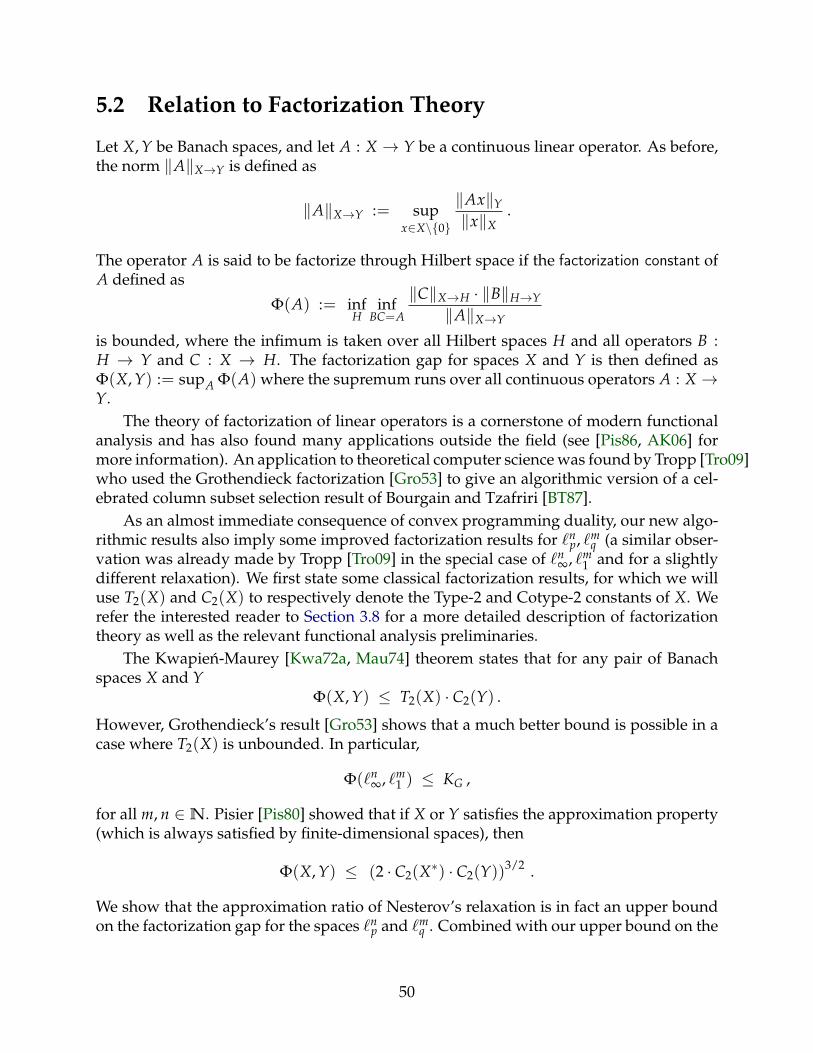
5.2 Relation to Factorization Theory
Let X, Y be Banach spaces, and let A : X → Y be a continuous linear operator. As before,the norm ‖A‖X→Y is defined as
‖A‖X→Y := supx∈X\0
‖Ax‖Y
‖x‖X.
The operator A is said to be factorize through Hilbert space if the factorization constant ofA defined as
Φ(A) := infH
infBC=A
‖C‖X→H · ‖B‖H→Y
‖A‖X→Y
is bounded, where the infimum is taken over all Hilbert spaces H and all operators B :H → Y and C : X → H. The factorization gap for spaces X and Y is then defined asΦ(X, Y) := supA Φ(A) where the supremum runs over all continuous operators A : X →Y.
The theory of factorization of linear operators is a cornerstone of modern functionalanalysis and has also found many applications outside the field (see [Pis86, AK06] formore information). An application to theoretical computer science was found by Tropp [Tro09]who used the Grothendieck factorization [Gro53] to give an algorithmic version of a cel-ebrated column subset selection result of Bourgain and Tzafriri [BT87].
As an almost immediate consequence of convex programming duality, our new algo-rithmic results also imply some improved factorization results for `n
p, `mq (a similar obser-
vation was already made by Tropp [Tro09] in the special case of `n∞, `m
1 and for a slightlydifferent relaxation). We first state some classical factorization results, for which we willuse T2(X) and C2(X) to respectively denote the Type-2 and Cotype-2 constants of X. Werefer the interested reader to Section 3.8 for a more detailed description of factorizationtheory as well as the relevant functional analysis preliminaries.
The Kwapien-Maurey [Kwa72a, Mau74] theorem states that for any pair of Banachspaces X and Y
Φ(X, Y) ≤ T2(X) · C2(Y) .
However, Grothendieck’s result [Gro53] shows that a much better bound is possible in acase where T2(X) is unbounded. In particular,
Φ(`n∞, `m
1 ) ≤ KG ,
for all m, n ∈N. Pisier [Pis80] showed that if X or Y satisfies the approximation property(which is always satisfied by finite-dimensional spaces), then
Φ(X, Y) ≤ (2 · C2(X∗) · C2(Y))3/2 .
We show that the approximation ratio of Nesterov’s relaxation is in fact an upper boundon the factorization gap for the spaces `n
p and `mq . Combined with our upper bound on the
50
integrality gap, we show an improved bound on the factorization constant, i.e., for anyp ≥ 2 ≥ q and m, n ∈N, we have that for X = `n
p, Y = `mq
Φ(X, Y) ≤ 1 + ε0
sinh−1(1)· (C2(X∗) · C2(Y)) ,
where ε0 ≤ 0.00863 as before. This improves on Pisier’s bound for all p ≥ 2 ≥ q, and forcertain ranges of (p, q) it also improves upon KG and the bound of Kwapien-Maurey.
5.3 Approximability and Factorizability
Let (Xn) and (Ym) be sequences of Banach spaces such that Xn is over the vector spaceRn and Ym is over the vector space Rm. We shall say a pair of sequences ((Xn), (Ym))factorize if Φ(Xn, Ym) is bounded by a constant independent of m and n. Similarly, weshall say a pair of families ((Xn), (Ym)) are computationally approximable if there existsa polynomial R(m, n), such that for every m, n ∈ N, there is an algorithm with runtimeR(m, n) approximating ‖A‖Xn→Ym within a constant independent of m and n (given anoracle for computing the norms of vectors and a separation oracle for the unit balls of thenorms). We consider the natural question of characterizing the families of norms that areapproximable and their connection to factorizability and Cotype.
The pairs (p, q) for which (`np, `m
q ) is known (resp. not known) to factorize, are pre-cisely those pairs (p, q) which are known to be computationally approximable (resp.inapproximable assuming hardness conjectures like P 6= NP and ETH). Moreover theHilbertian case which trivially satisfies factorizability, is also known to be computation-ally approximable (with approximation factor 1).
It is tempting to ask whether the set of computationally approximable pairs includesthe set of factorizable pairs or the pairs for which X∗n, Ym have bounded (independent ofm, n) Cotype-2 constant. Further yet, is there a connection between the approximationfactor and the factorization constant, or approximation factor and Cotype-2 constants (ofX∗n and Ym)? Our work gives some modest additional evidence towards such conjectures.Such a result would give credibility to the appealing intuitive idea of the approximationfactor being dependent on the “distance” to a Hilbert space.
5.4 Notation
For p ≥ 2 ≥ q ≥ 1, we will use the following notation: a := p∗ − 1 and b := q− 1. Wenote that a, b ∈ [0, 1].
For an m × n matrix M (or vector, when n = 1). For a scalar function f , we definef [M] to be the matrix with entries defined as ( f [M])i,j = f (Mi,j) for i ∈ [m], j ∈ [n]. Forvectors u, v ∈ R`, we denote by u v ∈ R` the entry-wise/Hadamard product of u and v.We denote the concatenation of two vectors u and v by u⊕ v.
For a function f (τ) = ∑k≥0 fk · τk defined as a power series, we denote by abs ( f ), thefunction abs ( f ) (τ) := ∑k≥0 | fk| · τk.
51
5.5 Analyzing the Approximation Ratio via Rounding
We will show that CP(A) is a good approximation to ‖A‖p→q by using an appropriategeneralization of Krivine’s rounding procedure. Before stating the generalized procedure,we shall give a more detailed summary of Krivine’s procedure.
5.5.1 Krivine’s Rounding Procedure
Krivine’s procedure centers around the classical random hyperplane rounding. In thiscontext, we define the random hyperplane rounding procedure on an input pair of matri-ces U ∈ Rm×`, V ∈ Rn×` as outputting the vectors sgn[Ug] and sgn[Vg] where g ∈ R` isa vector with i.i.d. standard Gaussian coordinates ( f [v] denotes entry-wise application ofa scalar function f to a vector v. We use the same convention for matrices.). The so-calledGrothendieck identity states that for vectors u, v ∈ R`,
E [sgn〈g , u〉 · sgn〈g , v〉] = sin−1〈u , v〉π/2
where u denotes u/‖u‖2. This implies the following equality which we will call the hy-perplane rounding identity:
E[sgn[Ug](sgn[Vg])T
]=
sin−1[UVT]
π/2. (5.1)
where for a matrix U, we use U to denote the matrix obtained by replacing the rows of Uby the corresponding unit (in `2 norm) vectors. Krivine’s main observation is that for anymatrices U, V, there exist matrices ϕ(U), ψ(V) with unit vectors as rows, such that
ϕ(U)ψ(V)T = sin[(π/2) · c · UVT]
where c = sinh−1(1) · 2/π. Taking U, V to be the optimal solution to CP(A), it followsthat
‖A‖∞→1 ≥⟨
A , E[sgn[ϕ(U) g] (sgn[ψ(V) g])T
]⟩= 〈A , c · UVT〉 = c · CP(A) .
The proof of Krivine’s observation follows from simulating the Taylor series of a scalarfunction using inner products. We will now describe this more concretely.
Observation 5.5.1 (Krivine). Let f : [−1, 1] → R be a scalar function satisfying f (ρ) =∑k≥1 fk ρk for an absolutely convergent series ( fk). Let abs ( f ) (ρ) := ∑k≥1 | fk| ρk and furtherfor vectors u, v ∈ R` of `2-length at most 1, let
SL( f , u) := (sgn( f1)√
f1 · u)⊕ (sgn( f2)√
f2 · u⊗2)⊕ (sgn( f3)√
f3 · u⊗3)⊕ · · ·SR( f , v) := (
√f1 · v)⊕ (
√f2 · v⊗2)⊕ (
√f3 · v⊗3)⊕ · · ·
52
Then for any U ∈ Rm×`, V ∈ Rn×`, SL( f ,√c f · U) and SR( f ,√c f · V) have `2-unit vectorsas rows, and
SL( f ,√
c f · U) SR( f ,√
c f · V)T = f [c f · UVT]
where SL( f , W) for a matrix W, is applied to row-wise and c f := (abs ( f )−1)(1).
Proof. Using the facts 〈y1 ⊗ y2 , y3 ⊗ y4〉 = 〈y1 , y3〉 · 〈y2 , y4〉 and〈y1 ⊕ y2 , y3 ⊕ y4〉 = 〈y1 , y3〉+ 〈y2 , y4〉, we have
- 〈SL( f , u) , SR( f , v)〉 = f (〈u , v〉)
- ‖SL( f , u)‖2 =√
abs ( f ) (‖u‖22)
- ‖SR( f , v)‖2 =√
abs ( f ) (‖v‖22)
The claim follows.
Before stating our full rounding procedure, we first discuss a natural generalizationof random hyperplane rounding, and much like in Krivine’s case this will guide the finalprocedure.
5.5.2 Generalizing Random Hyperplane Rounding – Hölder Dual Round-ing
Fix any convex bodies B1 ⊂ Rm and B2 ⊂ Rk. Suppose that we would like a strategy thatfor given vectors y ∈ Rm, x ∈ Rn, outputs y ∈ B1, x ∈ B2 so that yT A x = 〈A , y xT〉 isclose to 〈A , y xT〉 for all A. A natural strategy is to take
(y, x) := argmax(y,x)∈B1×B2
⟨y xT , y xT
⟩=
(argmax
y∈B1
〈y , y〉 , argmaxx∈B2
〈x , x〉)
In the special case where B is the unit `p ball, there is a closed form for an optimal solution
to maxx∈B〈x , x〉, given by Ψp∗(x)/‖x‖p∗−1p∗ , where Ψp∗(x) := sgn[x] |[x]|p∗−1. Note that
for p = ∞, this strategy recovers the random hyperplane rounding procedure. We shallcall this procedure, Gaussian Hölder Dual Rounding or Hölder Dual Rounding for short.
Just like earlier, we will first understand the effect of Hölder Dual Rounding on a solu-tion pair U, V. For ρ ∈ [−1, 1], let g1∼ρ g2 denote ρ-correlated standard Gaussians, i.e.,g1 = ρ g2 +
√1− ρ2 g3 where (g2, g3) ∼ N (0, I2), and let
fa, b(ρ) := Eg1∼ρg2
[sgn(g1)|g1|b sgn(g2)|g1|a
]We will work towards a better understanding of fa, b(·) in later sections. For now notethat we have for vectors u, v ∈ R`,
E[sgn〈g , u〉 |〈g , u〉|b · sgn〈g , v〉 |〈g , v〉|a
]= ‖u‖b
2 · ‖v‖a2 · fa, b(〈u , v 〉) .
53
Thus given matrices U, V, we obtain the following generalization of the hyperplane round-ing identity for Hölder Dual Rounding :
E[Ψq([Ug])Ψp∗([Vg])T
]= D(‖ui‖b
2)i∈[m]· fa, b([UVT]) · D(‖vj‖a
2)j∈[n]. (5.2)
5.5.3 Generalized Krivine Transformation and the Full Rounding Pro-cedure
We are finally ready to state the generalized version of Krivine’s algorithm. At a highlevel the algorithm simply applies Hölder Dual Rounding to a transformed version of theoptimal convex program solution pair U, V. Analogous to Krivine’s algorithm, the trans-formation is a type of “inverse” of Eq. (5.2).
(Inversion 1) Let (U, V) be the optimal solution to CP(A), and let (ui)i∈[m] and (vj)j∈[n]respectively denote the rows of U and V.
(Inversion 2) Let ca,b :=(
abs(
f−1a, b
))−1(1) and let
ϕ(U) := D(‖ui‖1/b
2 )i∈[m]SL( f−1
a, b ,√
ca,b · U) ,
ψ(V) := D(‖vj‖1/a
2 )j∈[n]SR( f−1
a, b ,√
ca,b · V) .
(Hölder-Dual 1) Let g ∼ N (0, I) be an infinite dimensional i.i.d. Gaussian vector.
(Hölder-Dual 2) Return y := Ψq(ϕ(U) g)/‖ϕ(U) g‖bq and x := Ψp∗(ψ(V) g)/‖ψ(V) g‖a
p∗ .
Remark 5.5.2. Note that ‖Ψr(x)‖r∗ = ‖x‖r−1r and so the returned solution pair always lie on
the unit `q∗ and `p spheres respectively.
Remark 5.5.3. Like in [AN04] the procedure above can be made algorithmic by observing thatthere always exist ϕ′(U) ∈ Rm×(m+n) and ψ′(V) ∈ Rm×(m+n), whose rows have the exact samelengths and pairwise inner products as those of ϕ(U) and ψ(V) above. Moreover they can becomputed without explicitly computing ϕ(U) and ψ(V) by obtaining the Gram decomposition of
M :=
abs(
f−1a, b
)[ca,b · VVT] f−1
a, b ([ca,b · UVT])
f−1a, b ([ca,b · VUT]) abs
(f−1a, b
)[ca,b · VVT]
,
and normalizing the rows of the decomposition according to the definition of ϕ(·) and ψ(·) above.The entries of M can be computed in polynomial time with exponentially (in m and n) goodaccuracy by implementing the Taylor series of f−1
a, b upto poly(m, n) terms (Taylor series inversioncan be done upto k terms in time poly(k)).
Remark 5.5.4. Note that the 2-norm of the i-th row (resp. j-th row) of ϕ(U) (resp. ψ(V)) is‖ui‖1/b
2 (resp. ‖vj‖1/a2 ).
We commence the analysis by defining some convenient normalized functions andwe will also show that ca,b above is well-defined.
54
5.5.4 Auxiliary Functions
Let fp, q(ρ) := fp, q(ρ)/(γp∗p∗ γ
qq), ha, b := abs
(f−1a, b
), and ha, b := abs
(f−1a, b
). Also note
that h−1a, b(ρ) = h−1
a, b(ρ)/(γp∗p∗ γ
qq).
Well Definedness. By Lemma 5.7.7, f−1a, b (ρ) and ha, b(ρ) are well defined for ρ ∈ [−1, 1].
By (M1) in Corollary 5.6.19, f−11 = 1 and hence ha, b(1) ≥ 1 and ha, b(−1) ≤ −1. Combin-
ing this with the fact that ha, b(ρ) is continuous and strictly increasing on [−1, 1], impliesthat h−1
a, b(x) is well defined on [−1, 1].
We can now proceed with the analysis.
5.5.5 1/(h−1p, q(1) · γp∗ γq) Bound on Approximation Factor
For any vector random variable X in a universe Ω, and scalar valued functions f1 : Ω→ R
and f2 : Ω→ (0, ∞). Let λ = E[ f1(X)]/E[ f2(X)]. Now we have
maxx∈Ω
f1(x)− λ · f2(x) ≥ E [ f1(X)− λ · f2(X)] = 0
⇒ maxx∈Ω
f1(x)/ f2(x) ≥ λ = E [ f1(X)] /E [ f2(X)] .
Thus we have
‖A‖p→q ≥E[〈A , Ψq(ϕ(U) g) Ψp∗(ψ(V) g)T〉]
E[‖Ψq(ϕ(U) g)‖q∗ · ‖Ψp∗(ψ(V) g)‖p]=〈A , E[Ψq(ϕ(U) g) Ψp∗(ψ(V) g)T]〉
E[‖Ψq(ϕ(U) g)‖q∗ · ‖Ψp∗(ψ(V) g)‖p],
which allows us to consider the numerator and denominator separately. We begin byproving the equality that the above algorithm was designed to satisfy:
Lemma 5.5.5. E[Ψq(ϕ(U) g) Ψp∗(ψ(V) g)T] = ca,b · (UVT)
Proof.
E[Ψq(ϕ(U) g) Ψp∗(ψ(V) g)T
]= D(‖ui‖2)i∈[m]
· fa, b([SL( f−1a, b ,√
ca,b · U) · SR( f−1a, b ,√
ca,b · V)T]) · D(‖vj‖2)j∈[n]
(by Eq. (5.2) and Remark 5.5.4)
= D(‖ui‖2)i∈[m]· fa, b([ f−1
a, b ([ca,b · UVT])]) · D(‖vj‖2)j∈[n]
(by Observation 5.5.1)
= D(‖ui‖2)i∈[m]· ca,b · UVT · D(‖vj‖2)j∈[n]
= ca,b ·UVT
55
It remains to upper bound the denominator which we do using a straightforwardconvexity argument.
Lemma 5.5.6. E[‖ϕ(U) g‖bq · ‖ψ(V) g‖a
p∗ ] ≤ γap∗ γb
q .
Proof.
E[‖ϕ(U) g‖b
q · ‖ψ(V) g‖ap∗]
≤ E[‖ϕ(U) g‖q∗b
q
]1/q∗ ·E
[‖ψ(V) g‖pa
p∗
]1/p
(1p+
1q∗≤ 1
)= E
[‖ϕ(U) g‖q
q]1/q∗ ·E
[‖ψ(V) g‖p∗
p∗
]1/p
=
∑i∈[m]
E[|N (0, ‖ui‖1/b
2 )|q]1/q∗
·
∑j∈[n]
E[|N (0, ‖vj‖1/a
2 )|p∗]1/p
(By Remark 5.5.4)
=
∑i∈[m]
‖ui‖q/b2
1/q∗
·
∑j∈[n]‖vj‖p∗/a
2
1/p
· γq/q∗q γ
p∗/pp∗
=
∑i∈[m]
‖ui‖q∗2
1/q∗
·
∑j∈[n]‖vj‖p
2
1/p
· γbq γa
p∗
= γbq γa
p∗ (feasibility of U, V)
We are now ready to prove our approximation guarantee.
Lemma 5.5.7. Consider any 1 ≤ q ≤ 2 ≤ p ≤ ∞. Then,
CP(A)
‖A‖p→q≤ 1/(γp∗ γq · h−1
a, b(1))
Proof.
‖A‖p→q ≥〈A , E[Ψq(ϕ(U) g) Ψp∗(ψ(V) g)T]〉
E[‖Ψq(ϕ(U) g)‖q∗ · ‖Ψp∗(ψ(V) g)‖p]
=〈A , E[Ψq(ϕ(U) g) Ψp∗(ψ(V) g)T]〉
E[‖ϕ(U) g‖bq · ‖ψ(V) g‖a
p∗ ](by Remark 5.5.2)
=ca,b · 〈A , UVT〉
E[‖ϕ(U) g‖bq · ‖ψ(V) g‖a
p∗ ](by Lemma 5.5.5)
=ca,b · CP(A)
E[‖ϕ(U) g‖bq · ‖ψ(V) g‖a
p∗ ](by optimality of U, V)
≥ ca,b · CP(A)
γap∗ γb
q(by Lemma 5.5.6)
56
=h−1
a, b(1) · CP(A)
γap∗ γb
q
= h−1a, b(1) · γp∗ γq · CP(A)
We next begin the primary technical undertaking of this chapter, namely provingupper bounds on h−1
p, q(1).
5.6 Hypergeometric Representation of fa, b(x)
In this section, we show that fa, b(ρ) can be represented using the Gaussian hypergeomet-ric function 2F1. The result of this section can be thought of as a generalization of theso-called Grothendieck identity for hyperplane rounding which simply states that
f0, 0(ρ) =π
2· E
g1∼ρ g2[sgn(g1) sgn(g2)] = sin−1(ρ)
We believe the result of this section and its proof technique to be of independent inter-est in analyzing generalizations of hyperplane rounding to convex bodies other than thehypercube.
Recall that fa, b(ρ) is defined as follows:
Eg1∼ρ g2
[sgn(g1)|g1|a sgn(g2)|g1|b
]where a = p∗ − 1 and b = q − 1. Our starting point is the simple observation that theabove expectation can be viewed as the noise correlation (under the Gaussian measure)of the functions f (a)(τ) := sgn τ · |τ|a and f (b)(τ) := sgn τ · |τ|b. Elementary Hermiteanalysis then implies that it suffices to understand the Hermite coefficients of f (a) andf (b) individually, in order to understand the Taylor coefficients of fa, b. To understand theHermite coefficients of f (a) and f (b) individually, we use a generating function approach.More specifically, we derive an integral representation for the generating function of the(appropriately normalized) Hermite coefficients which fortunately turns out to be closelyrelated to a well studied special function called the parabolic cylinder function.
Before proceeding, we require some preliminaries.
5.6.1 Hermite Analysis Preliminaries
Let γ denote the standard Gaussian probability distribution. For this section (and onlyfor this section), the (Gaussian) inner product for functions f , h ∈ (R, γ) → R is definedas
〈 f , h〉 :=∫
Rf (τ) · h(τ) dγ(τ) = E
τ∼N (0,1)[ f (τ) · h(τ)] .
Under this inner product there is a complete set of orthonormal polynomials (Hk)k∈N
defined below.
57
Definition 5.6.1. For a natural number k, then the k-th Hermite polynomial Hk : R→ R
Hk(τ) =1√k!· (−1) k · eτ2/2 · dk
dτk e−τ2/2 .
Any function f satisfying∫
R| f (τ)|2 dγ(τ) < ∞ has a Hermite expansion given by f =
∑k≥0 fk · Hk where fk = 〈 f , Hk〉 .
We have
Fact 5.6.2. Hk(τ) is an even (resp. odd) function when k is even (resp. odd).
We also have the Plancherel Identity (as Hermite polynomials form an orthonormalbasis):
Fact 5.6.3. For two real valued functions f and h with Hermite coefficients fk and hk, respectively,we have:
〈 f , h〉 = ∑k≥0
fk · hk .
The generating function of appropriately normalized Hermite polynomials satisfiesthe following identity:
e τλ−λ2/2 = ∑k≥0
Hk(τ) ·λk√
k!. (5.3)
Similar to the noise operator in Fourier analysis, we define the corresponding noiseoperator Tρ for Hermite analysis:
Definition 5.6.4. For ρ ∈ [−1, 1] and a real valued function f , we define the function Tρ f as:
(Tρ f )(τ) =∫
Rf(
ρ · τ +√
1− ρ2 · θ)
dγ(θ) = Eτ′∼ρ τ
[f (τ′)
].
Again similar to the case of Fourier analysis, the Hermite coefficients admit the fol-lowing identity:
Fact 5.6.5. (Tρ f )k = ρk · fk .
We recall that the fa, b(ρ) = Eg1∼ρ g2 [ f (a)(g1) · f (b)(g2))], where f (c)(τ) := sgn(τ) ·|τ|c for c ∈ a, b. As mentioned at the start of the section, we now note that fa, b(ρ) is thenoise correlation of f (a) and f (b). Thus we can relate the Taylor coefficients of fa, b(ρ), tothe Hermite coefficients of f (a) and f (b).
Claim 5.6.6 (Coefficients of fa, b(ρ)). For ρ ∈ [−1, 1], we have:
fa, b(ρ) = ∑k≥0
ρ2k+1 · f (a)2k+1 · f (b)
2k+1 ,
where f (a)i and f (b)
j are the i-th and j-th Hermite coefficients of f (a) and f (b), respectively.
Moreover, f (a)2k = f (b)
2k = 0 for k ≥ 0.
58
Proof. We observe that both f (a) and f (b) are odd functions and hence Fact 5.6.2 impliesthat f (a)
2k = f (b)2k = 0 for all k ≥ 0 – as f (a)(τ) · H2k(τ) is an odd function of τ.
fa, b(ρ) = Eg1∼ρ g2
[f (a)(g1) · f (b)(g2))
]= E
g1
[f (a)(g1) · Tρ f (b)(g1)
](Definition 5.6.4)
= 〈 f (a) , Tρ f (b)〉
= ∑k≥0
f (a)k · (Tρ f (b))k (Fact 5.6.3)
= ∑k≥0
f (a)2k+1 ·
(Tρ f (b))2k+1
= ∑k≥0
ρ2k+1 · f (a)2k+1 · f (b)
2k+1 (Fact 5.6.5) .
5.6.2 Hermite Coefficients of f (a) and f (b) via Parabolic Cylinder Func-tions
In this subsection, we use the generating function of Hermite polynomials to to obtain anintegral representation for the generating function of the (
√k! normalized) odd Hermite
coefficients of f (a) (and similarly of f (b)) is closely related to a special function calledthe parabolic cylinder function. We then use known facts about the relation betweenparabolic cylinder functions and confluent hypergeometric functions, to show that theHermite coefficients of f (c) can be obtained from the Taylor coefficients of a confluenthypergeometric function.
Before we state and prove the main results of this subsection we need some prelimi-naries:
Gamma, Hypergeometric and Parabolic Cylinder Function Preliminaries
For a natural number k and a real number τ, we denote the rising factorial as (τ)k :=τ · (τ + 1) · · · · (τ + k− 1). We now define the following fairly general classes of functionsand we later use them we obtain a Taylor series representation of fa, b(τ).
Definition 5.6.7. The confluent hypergeometric function with parameters α, β, and λ as:
1F1(α ; β ; λ) := ∑k
(α)k(β)k
· λk
k!.
The (Gaussian) hypergeometric function is defined as follows:
Definition 5.6.8. The hypergeometric function with parameters w, α, β and λ as:
2F1(w, α ; β ; λ) := ∑k
(w)k · (α)k(β)k
· λk
k!.
59
Next we define the Γ function:
Definition 5.6.9. For a real number τ, we define:
Γ(τ) :=∫ ∞
0tτ−1 · e−t dt .
The Γ function has the following property:
Fact 5.6.10 (Duplication Formula).
Γ(2τ)
Γ(τ)=
Γ(τ + 1/2)21−2τ
√π
We also note the relationship between Γ and γr:
Fact 5.6.11. For r ∈ [0, ∞),
γrr := E
g∼N (0,1)[|g|r] =
2r/2√
π· Γ(
1 + r2
).
Proof.
Eg∼N (0,1)
[|g|r]=
√2√π·∫ ∞
0|g|r · e−g2/2 dg
=
√2π· 2(r−1)/2 ·
∫ ∞
0
∣∣∣∣g2
2
∣∣∣∣(r−1)/2
· e−g2/2· g dg
=2r/2√
π· Γ(
1 + r2
)
Next, we record some facts about parabolic cylinder functions:
Fact 5.6.12 (12.5.1 of [Loz03]). Let U be the function defined as
U(α, λ) :=eλ2/4
Γ(
12 + α
) ∫ ∞
0tα−1/2 · e−(t+λ)2/2 dt ,
for all α such that IR(α) > −12 . The function U(α,±λ) is a parabolic cylinder function and is a
standard solution to the differential equation: d2wdλ2 −
(λ2
4 + α)
w = 0.
Next we quote the confluent hypergeometric representation of the parabolic cylinderfunction U defined above:
60
Fact 5.6.13 (12.4.1, 12.2.6, 12.2.7, 12.7.12, and 12.7.13 of [Loz03]).
U(α, λ) =
√π
2α/2+1/4 · Γ(3
4 +α2
) · eλ2/4 · 1F1
(−1
2α +
14
;12
; −λ2
2
)−
√π
2α/2−1/4 · Γ(
14 +
α2
) · λ · eλ2/4 · 1F1
(−α
2+
34
;32
; −λ2
2
)
Combining the previous two facts, we get the following:
Corollary 5.6.14. For all real α > −12 , we have:
∫ ∞
0tα−1/2 · e−(t+λ)2/2 dt =
√π · Γ
(12 + α
)2α/2+1/4 · Γ
(34 +
α2
) · 1F1
(−α
2+
14
;12
; −λ2
2
)
−
√π · Γ
(12 + α
)2α/2−1/4 · Γ
(14 +
α2
) · λ · 1F1
(−α
2+
34
;32
; −λ2
2
).
Generating Function of Hermite Coefficients and its Confluent Hypergeometric Rep-resentation
Using the generating function of (appropriately normalized) Hermite polynomials, wederive an integral representation for the generating function of the (appropriately nor-malized) Hermite coefficients of f (a) (and similarly f (b)):
Lemma 5.6.15. For c ∈ a, b, let f (c)k denote the k-th Hermite coefficient of f (c)(τ) :=
sgn (τ) · |τ|c. Then we have the following identity:
∑k≥0
λ2k+1√(2k + 1)!
· f (c)2k+1 =
1√2π
∫ ∞
0τc ·
(e−(τ−λ)2/2 − e−(τ+λ)2/2
)dτ .
Proof. We observe that for, f (c) is an odd function and hence Fact 5.6.2 implies thatf (c)(τ) ·H2k(τ) is an odd function and f (c)(τ) ·H2k+1(τ) is an even function. This impliesfor any k ≥ 0, that f (c)
2k = 0 and
f (c)2k+1 =
1√2π
∫ ∞
−∞sgn (τ) · τc · H2k+1(τ) · e−τ2/2 dτ =
√2π
∫ ∞
0τc · H2k+1(τ) · e−τ2/2 dτ .
Thus we have
∑k≥0
λ2k+1√(2k + 1)!
· f (c)2k+1
=
√2π· ∑
k≥0
∫ ∞
0τc · e−τ2/2 · H2k+1(τ) ·
λ2k+1√(2k + 1)!
dτ
61
=
√2π·∫ ∞
0τc · e−τ2/2 ∑
k≥0H2k+1(τ) ·
λ2k+1√(2k + 1)!
dτ (see below)
=1√2π·∫ ∞
0τc · e−τ2/2 ·
(eτλ−λ2/2 − e−τλ−λ2/2
)dτ ( by Eq. (5.3))
=1√2π·∫ ∞
0τc ·
(e−(τ−λ)2/2 − e−(τ+λ)2/2
)dτ
where the exchange of summation and integral in the second equality follows by Fu-bini’s theorem. We include this routine verification for the sake of completeness. As aconsequence of Fubini’s theorem, if ( fk : R → R)k is a sequence of functions such that∑k≥0
∫ ∞0 | fk| < ∞, then ∑k≥0
∫ ∞0 fk =
∫ ∞0 ∑k≥0 fk . Now for any fixed k, we have∫ ∞
0τc · |Hk(x)| dγ(τ) ≤
(∫ ∞
0τ2c dγ(τ)
)1/2
·(∫ ∞
0|Hk(x)|2 dγ(τ)
)1/2
≤ γc2c < ∞ .
Setting fk(τ) := τc · e−τ2/2 · H2k+1(τ) · λ2k+1/√(2k + 1)! , we get that ∑k≥0
∫ ∞0 | fk| < ∞.
This completes the proof.
Finally using known results about parabolic cylinder functions, we are able to re-late the aforementioned integral representation to a confluent hypergeometric function(whose Taylor coefficients are known).
Lemma 5.6.16. For λ ∈ [−1, 1] and real valued c > −1, we have
1√2π
∫ ∞
0τc(
e−(τ−λ)2/2 − e−(τ+λ)2/2)
dτ = γc+1c+1 · λ · 1F1
(1− c
2;
32
; −λ2
2
)Proof. We prove this by using the Corollary 5.6.14 with a = c + 1
2 . We note that α > −12
and 1F1(·, ·,−λ2/2
)is an even function of λ. So combining the two, we get:
1√2π
∫ ∞
0τc(
e−(τ−λ)2/2 − e−(τ+λ)2/2)
dτ
=2√2π·√
π · Γ (c + 1)
2c/2 · Γ(
c+12
) · λ · 1F1
(− c
2+
12
;32
;−12
λ2)
= 2(1−c)/2 ·Γ(
c+12 + 1
2
)2−c ·
√π· λ · 1F1
(1− c
2;
32
; −λ2
2
)(by Fact 5.6.10)
= γc+1c+1 · λ · 1F1
(1− c
2;
32
; −λ2
2
)(by Fact 5.6.11)
5.6.3 Taylor Coefficients of fa, b(x) and Hypergeometric Representation
By Claim 5.6.6, we are left with understanding the function whose power series is givenby a weighted coefficient-wise product of a certain pair of confluent hypergeometric func-tions. This turns out to be precisely the Gaussian hypergeometric function, as we will seebelow.
62
Observation 5.6.17. Let fk := [τk] 1F1(a1, 3/2, τ) and hk := [τk] 1F1(b1, 3/2, τ). Further letµk := fk · hk · (2k + 1)!/4k. Then for ρ ∈ [−1, 1],
∑k≥0
µk · ρn = 2F1(a1, b1 ; 3/2 ; ρ) .
Proof. The claim is equivalent to showing that µk = (a1)k (b1)k/((3/2)k k!). Since wehave fk = (a1)k/((3/2)k k!) and hk = (b1)k/((3/2)k k!), it is sufficient to show that (2k +1)!/4k = (3/2)k · k!. Indeed we have,
(2k + 1)! = 2k · k! · 1 · 3 · 5 · · · (2k + 1)
= 4k · k! · 32· 5
2· · ·(
32+ k− 1
)= 4k · k! · (3/2)k .
We are finally equipped to put everything together.
Theorem 5.6.18. For any a, b ∈ (−1, ∞) and ρ ∈ [−1, 1], we have
fa, b(ρ) :=1
γa+1a+1 · γ
b+1b+1
· Eg1∼ρ g2
[sgn(g1)|g1|a sgn(g2)|g1|b
]= ρ · 2F1
(1− a
2,
1− b2
;32
; ρ2)
.
It follows that the (2k + 1)-th Taylor coefficient of fa, b(ρ) is
((1− a)/2)k ((1− b)/2)k((3/2)k k!)
.
Proof. The claim follows by combining Claim 5.6.6, Lemmas 5.6.15 and 5.6.16, and Obser-vation 5.6.17.
This hypergeometric representation immediately yields some non-trivial coefficientand monotonicity properties:
Corollary 5.6.19. For any a, b ∈ [0, 1], the function fa, b : [−1, 1]→ R satisfies
(M1) [ρ] fa, b(ρ) = 1 and [ρ3] fa, b(ρ) = (1− a)(1− b)/6.
(M2) All Taylor coefficients are non-negative. Thus fa, b(ρ) is increasing on [−1, 1].
(M3) All Taylor coefficients are decreasing in a and in b. Thus for any fixed ρ ∈ [−1, 1], fa, b(ρ)is decreasing in a and in b.
(M4) Note that fa, b(0) = 0 and by (M1) and (M2), fa, b(1) ≥ 1. By continuity, fa, b([0, 1])contains [0, 1]. Combining this with (M3) implies that for any fixed ρ ∈ [0, 1], f−1
a, b (ρ) isincreasing in a and in b.
63
5.7 sinh−1(1)/(1 + ε0) Bound on h−1a, b(1)
In this section we show that p = ∞, q = 1 (the Grothendieck case) is roughly the extremalcase for the value of h−1
a, b(1), i.e., we show that for any 1 ≤ q ≤ 2 ≤ p ≤ ∞, h−1a, b(1) ≥
sinh−1(1)/(1+ ε0) (recall that h−10, 0(1) = sinh−1(1)). While we were unable to establish as
much, we conjecture that h−1a, b(1) ≥ sinh−1(1). Section 5.7.1 details some of the challenges
involved in establishing that sinh−1(1) is the worst case, and presents our approach toestablish an approximate bound, which will be formally proved in Section 5.7.2.
5.7.1 Behavior of The Coefficients of f−1a, b (z).
Krivine’s upper bound on the real Grothendieck constant, Haagerup’s upper bound [Haa81]on the complex Grothendieck constant and the work of Naor and Regev [NR14, BdOFV14]on the optimality of Krivine schemes are all closely related to our work in that each ofthe aforementioned papers needs to lower bound (abs
(f−1))−1(1) for an appropriate
odd function f (the work of Briet et al. [BdOFV14] on the rank-constrained Grothendieckproblem is also a generalization of Krivine’s and Haagerup’s work, however they didnot derive a closed form upper bound on (abs
(f−1))−1(1) in their setting). In Krivine’s
setting f = sin−1 x, implying (abs(
f−1))−1 = sinh−1 and hence the bound is immedi-ate. In our setting, as well as in [Haa81] and [NR14, BdOFV14], f is given by its Taylorcoefficients and is not known to have a closed form. In [NR14], all coefficients of f−1
subsequent to the third are negligible and so one doesn’t incur much loss by assumingthat abs
(f−1) (ρ) = c1ρ + c3ρ3. In [Haa81], the coefficient of ρ in f−1(ρ) is 1 and ev-
ery subsequent coefficient is negative, which implies that abs(
f−1) (ρ) = 2ρ − f−1(ρ).Note that if the odd coefficients of f−1 are alternating in sign like in Krivine’s setting,then abs
(f−1) (ρ) = −i · f−1(iρ). These structural properties of the coefficients help their
analyses.In our setting there does not appear to be such a strong relation between (abs
(f−1))
and f−1. Consider f (ρ) = fa, a(ρ). For certain a ∈ (0, 1), the sign pattern of the coeffi-cients of f−1 is unlike that of [Haa81] or sin ρ. In fact empirical results suggest that theodd coefficients of f alternate in sign up to some term K = K(a), and subsequently the co-efficients are all non-positive (where K(a)→ ∞ as a→ 0), i.e., the sign pattern appears tobe interpolating between that of sin ρ and that of f−1(ρ) in the case of Haagerup [Haa81].
Another source of difficulty is that for a fixed a, the coefficients of f−1 (with andwithout magnitude) are not necessarily monotone in k, and moreover for a fixed k, thek-th coefficient of f−1 is not necessarily monotone in a.
A key part of our approach is noting that certain milder assumptions on the coeffi-cients are sufficient to show that sinh−1(1) is the worst case. The proof crucially uses themonotonicity of fa, b(ρ) in a and b. The conditions are as follows:
Let f −1k := [ρk] f−1
a, b (ρ). Then
64
(C1) f −1k ≤ 1/k! if k (mod 4) ≡ 1.
(C2) f −1k ≤ 0 if k (mod 4) ≡ 3.
To be more precise, we were unable to establish that the above conditions hold for all k(however we conjecture that it is true for all k), and instead use Mathematica to verifyit for the fist few coefficients. We additionally show that the coefficients of f−1
a, b decayexponentially. Combining this exponential decay with a robust version of the previouslyadvertised claim yields that h−1
a, b(1) ≥ sinh−1(1)/(1 + ε0).We next proceed to prove the claim that the aforementioned conditions are sufficient
to show that sinh−1(1) is the worst case. We will need the following definition. For anodd positive integer t, let
herr(t, ρ) := ∑k≥t| f −1
k | · ρk
Lemma 5.7.1. If t is an odd integer such that (C1) and (C2) are satisfied for all k < t, andρ = sinh−1(1− 2herr(t, δ)) for some δ ≥ ρ, then ha, b(ρ) ≤ 1.
Proof. We have,
ha, b(ρ)
= ∑k≥1| f −1
k | · ρk
= − f−1a, b (ρ) + ∑
k≥1max2 f −1
k , 0 · ρk
= − f−1a, b (ρ) + ∑
1≤k<tk mod 4≡1
max2 f −1k , 0 · ρk + ∑
k≥tmax2 f −1
k , 0 · ρk (by (C2))
≤ − f−1a, b (ρ) + ∑
1≤k<tk mod 4≡1
max2 f −1k , 0 · ρk + 2 herr(t, ρ)
≤ − f−1a, b (ρ) + sin(ρ) + sinh(ρ) + 2 herr(t, ρ) (by (C1))
≤ − f−1a, b (ρ) + sin(ρ) + 1 + 2(herr(t, ρ)− herr(t, δ)) ( ρ = sinh−1(1− 2herr(t, δ)) )
≤ − f−1a, b (ρ) + sin(ρ) + 1 (ρ ≤ δ)
≤ − f−10, 0(ρ) + sin(ρ) + 1 (Corollary 5.6.19 : (M4))
= 1 ( f−10, 0(ρ) = sin(ρ))
Thus we obtain,
Theorem 5.7.2. For any 1 ≤ q ≤ 2 ≤ p ≤ ∞, let a := p∗ − 1, b = q − 1. Then for anym, n ∈N and A ∈ Rm×n, CP(A)/‖A‖p→q ≤ 1/(h−1
a, b(1) · γq γp∗) and moreover
- h−11, b(1) = h−1
a, 1(1) = 1.
65
- h−1a, b(1) ≥ sinh−1(1)/(1 + ε0) where ε0 = 0.00863.
Proof. The first inequality follows from Lemma 5.5.7. As for the next item, If p = 2 orq = 2 (i.e., a = 1 or b = 1) we are trivially done since h−1
a, b(ρ) = ρ in that case (since fork ≥ 1, (0)k = 0). So we may assume that a, b ∈ [0, 1).
We are left with proving the final part of the claim. Now using Mathematica we verify(exactly)1 that (C1) and (C2) are true for k ≤ 29. Now let δ = sinh−1(0.974203). Thenby Lemma 5.7.7 (which states that f −1
k decays exponentially and will be proven in thesubsequent section),
herr(31, δ) := ∑k≥31| f −1
k | · dk ≤ 6.1831
31· δ31
1− δ2 ≤ 0.0128991 . . . .
Now by Lemma 5.7.1 we know h−1a, b(1) ≥ sinh−1(1− 2herr(31, δ)). Thus,
h−1a, b(1) ≥ sinh−1(0.974202) ≥ sinh−1(1)/(1 + ε0) for ε0 = 0.00863, which completes the
proof.
5.7.2 Bounding Inverse Coefficients
In this section we prove that f −1k decays as 1/ck for some c = c(a, b) > 1, proving
Lemma 5.7.7. Throughout this section we assume 1 ≤ p∗, q < 2, and a = p∗− 1, b = q− 1(i.e., a, b ∈ [0, 1)). Via the power series representation, fa, b(z) can be analytically contin-ued to the unit complex disk. Let f−1
a, b (z) be the inverse of fa, b(z) and recall f −1k denotes
its k-th Taylor coefficient.We begin by stating a standard identity from complex analysis that provides a conve-
nient contour integral representation of the Taylor coefficients of the inverse of a function.We include a proof for completeness.
Lemma 5.7.3 (Inversion Formula). There exists δ > 0, such that for any odd k,
f −1k =
2πk=(∫
C+δ
fa, b(z)−k dz)
(5.4)
where C+δ denotes the first quadrant quarter circle of radius δ with counter-clockwise orientation.
Proof. Via the power series representation, fa, b(z) can be analytically continued to theunit complex disk. Thus by inverse function theorem for holomorphic functions, thereexists δ0 ∈ (0, 1] such that fa, b(z) has an analytic inverse in the open disk |z| < δ0. Sofor δ ∈ (0, δ0), fa, b(Cδ) is a simple closed curve with winding number 1 (where Cδ isthe complex circle of radius δ with the usual counter-clockwise orientation). Thus byCauchy’s integral formula we have
f −1k =
12πi
∫fa, b(Cδ)
f−1a, b (w)
w k dw =1
2πi
∫Cδ
z · f ′a, b(z)
fa, b(z)k+1 dz
1 We generated f −1k as a polynomial in a and b and maximized it over a, b ∈ [0, 1] using the Mathematica
“Maximize” function which is exact for polynomials.
66
where the second equality follows from substituting w = fa, b(z).Now by Fact 5.7.5, z/ fa, b(z)k is holomorphic on the open set |z| ∈ (0, 1), which
contains Cδ. Hence by the fundamental theorem of contour integration we have
∫Cδ
ddz
(z
fa, b(z)k
)dz = 0 ⇒
∫Cδ
z · f ′a, b(z)
fa, b(z)k+1 dz =1k
∫Cδ
1fa, b(z)k dz
So we get,
f −1k =
12πik
∫Cδ
fa, b(z)−k dz =1
2πk=(∫
Cδ
fa, b(z)−k dz)
where the second equality follows since f −1k is purely real. Lastly, we complete the proof
of the claim by using the fact that for odd k, fa, b(z)−k is odd and that fa, b(z) = fa, b(z).
We next state a standard bound on the magnitude of a contour integral that we willuse in our analysis.
Fact 5.7.4 (ML-inequality). If f is a complex valued continuous function on a contour Γ and| f (z)| is bounded by M for every z ∈ Γ, then∣∣∣∣∫Γ
f (z)∣∣∣∣ ≤ M · `(Γ)
where `(Γ) is the length of Γ.
Unfortunately the integrand in Eq. (5.4) can be very large for small δ, and we can-not use the ML-inequality as is. To fix this, we modify the contour of integration (usingCauchy’s integral theorem) so that the imaginary part of the integral vanishes when re-stricted to the sections close to the origin, and the integrand is small in magnitude on thesections far from the origin (thus allowing us to use the ML-inequality). To do this wewill need some preliminaries.
fa, b(z) is defined on the closed complex unit disk. The domain is analytically ex-tended to the region C \ ((−∞,−1)∪ (1, ∞)), using the Euler-type integral representationof the hypergeometric function.
f+a, b(z) := B(
1− b2
, 1 +b2
)−1
· I(z)
where B(τ1, τ2) is the beta function and
I(z) := z∫ 1
0
(1− t)b/2 dtt(1+b)/2 · (1− z2t)(1−a)/2
.
Fact 5.7.5. For any a1 > 0, 2F1(a1, b1, c1, z) has no non-zero roots in the region C \ (1, ∞). Thisimplies that if p∗ < 2, f+a, b(z) has no non-zero roots in the region C \ ((−∞,−1) ∪ (1, ∞)).
67
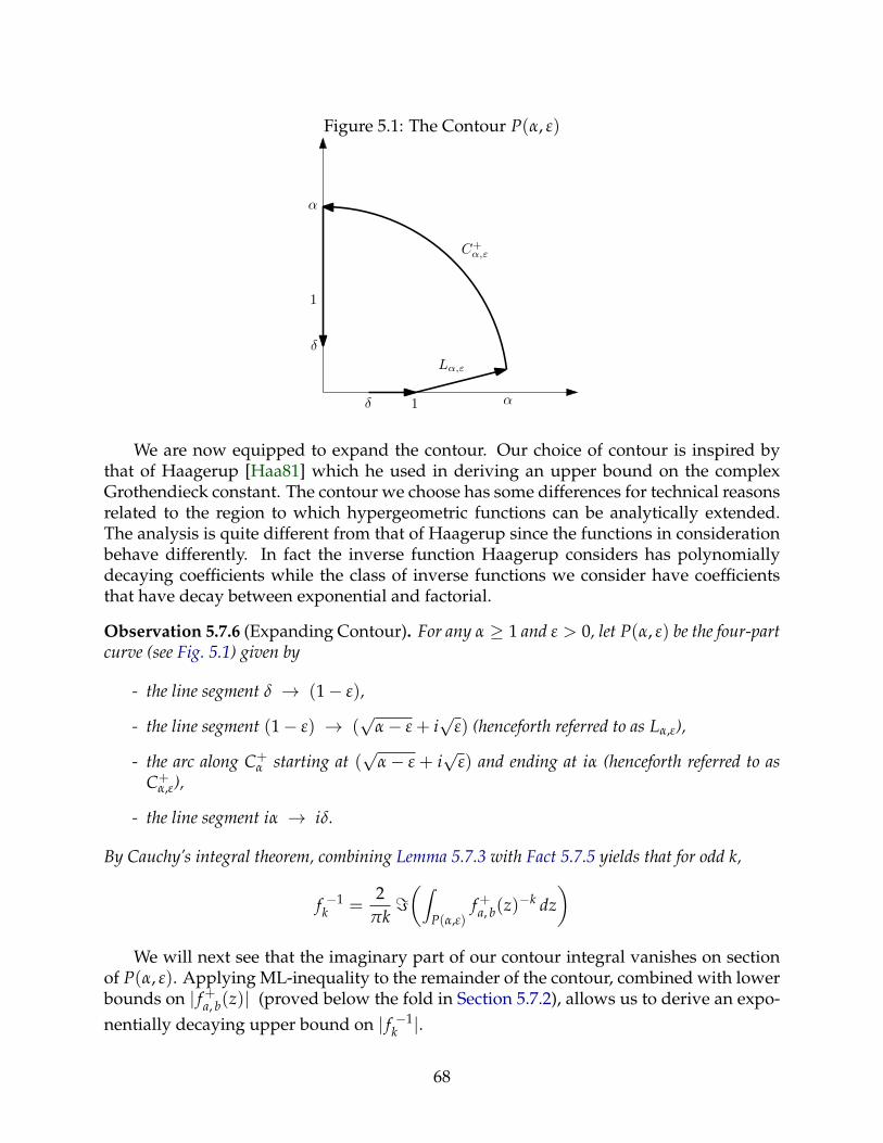
Figure 5.1: The Contour P(α, ε)
δ 1 α
δ
1
α
Lα,ε
C+α,ε
We are now equipped to expand the contour. Our choice of contour is inspired bythat of Haagerup [Haa81] which he used in deriving an upper bound on the complexGrothendieck constant. The contour we choose has some differences for technical reasonsrelated to the region to which hypergeometric functions can be analytically extended.The analysis is quite different from that of Haagerup since the functions in considerationbehave differently. In fact the inverse function Haagerup considers has polynomiallydecaying coefficients while the class of inverse functions we consider have coefficientsthat have decay between exponential and factorial.
Observation 5.7.6 (Expanding Contour). For any α ≥ 1 and ε > 0, let P(α, ε) be the four-partcurve (see Fig. 5.1) given by
- the line segment δ → (1− ε),
- the line segment (1− ε) → (√
α− ε + i√
ε) (henceforth referred to as Lα,ε),
- the arc along C+α starting at (
√α− ε + i
√ε) and ending at iα (henceforth referred to as
C+α,ε),
- the line segment iα → iδ.
By Cauchy’s integral theorem, combining Lemma 5.7.3 with Fact 5.7.5 yields that for odd k,
f −1k =
2πk=(∫
P(α,ε)f+a, b(z)
−k dz)
We will next see that the imaginary part of our contour integral vanishes on sectionof P(α, ε). Applying ML-inequality to the remainder of the contour, combined with lowerbounds on | f+a, b(z)| (proved below the fold in Section 5.7.2), allows us to derive an expo-nentially decaying upper bound on | f −1
k |.
68
Lemma 5.7.7. For any 1 ≤ p∗, q < 2, there exists ε > 0 such that
| f −1k | ≤
6.1831k(1 + ε)k .
Proof. For a contour P, we define V(P) as
V(P) :=2
πk=(∫
Pf+a, b(z)
−k dz)
As is evident from the integral representation, f+a, b(z) is purely imaginary if z is purelyimaginary, and as is evident from the power series, fa, b(z) is purely real if z lies on thereal interval [−1, 1]. This implies that V(δ→ (1− ε)) = V(iα→ iδ) = 0.
Now combining Fact 5.7.4 (ML-inequality) with Lemma 5.7.9 and Lemma 5.7.12 (whichstate that the integrand is small in magnitude over C+
6,ε and L6,ε respectively), we get thatfor sufficiently small ε > 0,
|V(P(6, ε))| ≤ |V(C+6,ε)|+ |V(L6,ε)|
≤ 2πk· 3π/2(1 + ε)k +
2πk· 6− 1 + O(
√ε)
(1 + ε)k
≤ 6.1831k(1 + ε)k . (taking ε sufficiently small)
Lower bounds on | f+a, b(z)| Over C+α,ε and Lα,ε
In this section we show that for sufficiently small ε, | f+a, b(z)| > 1 over Lα,ε (regardlessof the value of α, Lemma 5.7.12), and over C+
α,ε when α is a sufficiently large constant(Lemma 5.7.9).
We will first show the claim for C+α,ε by relating | f+a, b(z)| to |z|. While the asymptotic
behavior of hypergeometric functions for |z| → ∞ has been extensively studied (see forinstance [Loz03]), it appears that our desired estimates aren’t immediate consequences ofprior work for two reasons. Firstly, we require relatively precise estimates for moderatelylarge but constant |z|. Secondly, due to the expressive power of hypergeometric functions,the estimates we derive can only be true for hypergeometric functions parameterized in aspecific range. Indeed, our proof crucially uses the fact that a, b ∈ [0, 1). Our approach isto use the Euler-type integral representation of f+a, b(z) which as a reminder to the readeris as follows:
f+a, b(z) := B(
1− b2
, 1 +b2
)−1
· I(z)
where B(x, y) is the beta function and
I(z) := z∫ 1
0
(1− t)b/2 dtt(1+b)/2 · (1− z2t)(1−a)/2
.
69
We start by making the simple observation that the integrand of I(z) is always in thepositive complex quadrant — an observation that will come in handy multiple times inthis section, in dismissing the possibility of cancellations. This is the part of our proof thatmakes the most crucial use of the assumption that 0 ≤ a < 1 (equivalently 1 ≤ p∗ < 2).
Observation 5.7.8. Let z = reiθ be such that either one of the following two cases is satisfied:
(A) r < 1 and θ = 0.
(B) θ ∈ (0, π/2].
Then for any 0 ≤ a ≤ 1 and any t ∈ R+,
arg(
z(1− tz2)(1−a)/2
)∈ [0, π/2]
Proof. The claim is clearly true when θ = 0 and r < 1. It is also clearly true when θ = π/2.Thus we may assume θ ∈ (0, π/2).
arg(z) ∈ (0, π/2) ⇒ arg(−tz2) ∈ (−π, 0) ⇒ =(−tz2) < 0
⇒ =(1− tz2) < 0 ⇒ arg(1− tz2) ∈ (−π, 0)
Moreover since arg(−tz2) = 2θ − π ∈ (−π, 0), we have arg(1− tz2) > 2θ − π. Thus wehave,
arg(1− tz2) ∈ (2θ − π, 0) ⇒ arg((1− tz2)(1−a)/2
)∈ ((1− a)(θ − π/2), 0)
⇒ arg(
1/(1− tz2)(1−a)/2)∈ (0, (1− a)(π/2− θ))
⇒ arg(
z/(1− tz2)(1−a)/2)∈ (0, (1− a)(π/2− θ) + θ) ⊆ (0, π/2)
We now show | f+a, b(z)| is large over C+α,ε. The main idea is to move from a complex
integral to a real integral with little loss, and then estimate the real integral. To do this,we use Observation 5.7.8 to argue that the magnitude of I(z) is within
√2 of the integral
of the magnitude of the integrand.
Lemma 5.7.9 ( | f+a, b(z)| is large over C+α,ε ). Assume a, b ∈ [0, 1) and consider any z ∈ C with
|z| ≥ 6. Then | f+a, b(z)| > 1.
Proof. We start with a useful substitution.
I(z) = z∫ 1
0
(1− t)b/2 dtt(1+b)/2 · (1− z2t)(1−a)/2
= rbeiθ∫ r2
0
(1− s/r2)b/2 dss(1+b)/2 · (1− e2iθs)(1−a)/2
(Subst. s = r2t, where z = reiθ)
= rb∫ r2
0
wa(s, θ) · (1− s/r2)b/2 dss1+(b−a)/2
70
where
wa(s, θ) :=eiθ
(1/s− e2iθ)(1−a)/2.
We next exploit the observation that the integrand is always in the positive complexquadrant by showing that |I(z)| is at most a factor of
√2 away from the integral obtained
by replacing the integrand with its magnitude.
|I(z)|
=√
IR(I(z))2 +=(I(z))2
≥ (|IR(I(z))|+ |=(I(z))|)/√
2 (Cauchy-Schwarz)
= (IR(I(z)) +=(I(z)))/√
2 (by Observation 5.7.8)
=rb√
2
∫ r2
0(IR(wa(s, θ)) +=(wa(s, θ))) · (1− s/r2)b/2 ds
s1+(b−a)/2
=rb√
2
∫ r2
0(|IR(wa(s, θ))|+ |=(wa(s, θ))|) · (1− s/r2)b/2 ds
s1+(b−a)/2(by Observation 5.7.8)
≥ rb√
2
∫ r2
0|wa(s, θ)| · (1− s/r2)b/2 ds
s1+(b−a)/2(‖v‖1 ≥ ‖v‖2)
≥ rb√
2
∫ r2
0
1(1 + 1/s)(1−a)/2
· (1− s/r2)b/2 dss1+(b−a)/2
We now break the integral into two parts and analyze them separately. We start by ana-lyzing the part that’s large when b→ 0.
rb√
2
∫ r2
1
1(1 + 1/s)(1−a)/2
· (1− s/r2)b/2 dss1+(b−a)/2
≥ rb
2
∫ r2
1
(1− s/r2)b/2 dss1+(b−a)/2
≥ rb
2
∫ r2/2
1
(1− s/r2)b/2 dss1+(b−a)/2
≥ rb
2√
2
∫ r2/2
1
dss1+(b−a)/2
(since s ≤ r2/2)
≥ rb ·min1, ra−b2√
2
∫ r2/2
1
dss
=minra, rb · log(r2/2)
2√
2
≥ log(r/√
2)√2
71
We now analyze the part that’s large when b→ 1.
rb√
2
∫ 1
0
1(1 + 1/s)(1−a)/2
· (1− s/r2)b/2 dss1+(b−a)/2
=rb√
2
∫ 1
0
(1− s/r2)b/2
(1 + s)(1−a)/2· ds
s(1+b)/2
≥ rb ·√
1− 1/r2
2
∫ 1
0
dss(1+b)/2
(since s ≤ 1)
=rb ·√
1− 1/r2
1− b
Combining the two estimates above yields that if r >√
2,
| f+a, b(z)| ≥ B(
1− b2
, 1 +b2
)−1
·(
log(r/√
2)√2
+rb ·√
1− 1/r2
1− b
)Lastly, the proof follows by using the following estimate:
Fact 5.7.10. Via Mathematica, for 0 ≤ b < 1 we have
B(
1− b2
, 1 +b2
)−1
·(
log(6/√
2)√2
+6b ·√
1− 1/62
1− b
)≥ 1.003
Remark 5.7.11. The preceding proof can be used to derive the precise asymptotic behavior of| f+a, b(z)| in r. Specifically, it grows as ra log r if a = b and as r maxa,b if a 6= b.
We now show that | f+a, b(z)| > 1 over Lα,ε. To do this, it is insufficient to assume that|z| ≥ 1 since there exist points z (for instance z = i) of unit length such that | f+a, b(z)| < 1.To show the claim, we observe that | f+a, b(z)| is large when z is close to the real line anduse the fact that Lα,ε is close to the real line. Formally, we show that if z is of length atleast 1 and is sufficiently close to the real line, | f+a, b(z)| is close to f+a, b(1). Lastly, we usethe power series representation of the hypergeometric function to obtain a sufficientlyaccurate lower bound on f+a, b(1).
Lemma 5.7.12 ( | f+a, b(z)| is large over Lα,ε ). Assume a, b ∈ [0, 1) and consider any γ ≥ 1− ε1.Let ε2 :=
√ε1 and z := γ(1 + iε1). Then for ε1 > 0 sufficiently small, | f+a, b(z)| > 1.
Proof. Below the fold we will show
|I(z)| ≥ (1−O(√
ε1))∫ 1−ε2
0
(1− s)b/2 dss(1+b)/2 · (1− s)(1−a)/2
(5.5)
But we know (LHS, RHS refer to Eq. (5.5))
B(
1− b2
, 1 +b2
)−1
· LHS = f+a, b(z) and
72
B(
1− b2
, 1 +b2
)−1
· RHS → fa, b(1) as ε1 → 0
Also by Corollary 5.6.19 : (M1), (M2), fa, b(1) ≥ 1 + (1− a)(1− b)/6 > 1. Thus for ε1sufficiently small, we must have | f+a, b(z)| > 1.
We now show Eq. (5.5), by comparing integrands point-wise. To do this, we willassume the following closeness estimate that we will prove below the fold:
IR(
1 + iε1
(1− s(1 + iε1)2)(1−a)/2
)=
1−O(ε2)
(1− s)(1−a)/2. (5.6)
We will also need the following inequality. Since γ ≥ 1− ε1 = 1− ε22, for any 0 ≤ s ≤
1− ε2, we have(1− s/γ2)b/2 ≥ (1−O(ε2)) · (1− s)b/2. (5.7)
Given, these estimates, we can complete the proof of Eq. (5.5) as follows:
IR(I(z))
= IR
(z∫ 1
0
(1− t)b/2 dtt(1+b)/2 · (1− tz2)(1−a)/2
)
= IR
(γb(1 + iε1)
∫ γ2
0
(1− s/γ2)b/2 dss(1+b)/2 · (1− s(1 + iε1)2)(1−a)/2
)(subst. s← γ2t)
≥ IR
(γb(1 + iε1)
∫ 1−ε2
0
(1− s/γ2)b/2 dss(1+b)/2 · (1− s(1 + iε1)2)(1−a)/2
)(by Observation 5.7.8)
= γb∫ 1−ε2
0IR(
1 + iε1
(1− s(1 + iε1)2)(1−a)/2
)(1− s/γ2)b/2 ds
s(1+b)/2
≥ (1−O(ε2)) · γb∫ 1−ε2
0
(1− s/γ2)b/2 dss(1+b)/2 · (1− s)(1−a)/2
(by Eq. (5.6))
≥ (1−O(ε2))∫ 1−ε2
0
(1− s)b/2 dss(1+b)/2 · (1− s)(1−a)/2
(by Eq. (5.7), γ ≥ 1− ε1)
It remains to establish Eq. (5.6), which we will do by considering the numerator andreciprocal of the denominator separately and subsequently using the fact that IR(z1z2) =IR(z1)IR(z2)− =(z1)=(z2). In doing this, we need to show that the respective real partsare large and respective imaginary parts are small for which the following simple factswill come in handy.
Fact 5.7.13. Let z = reiθ be such that IRz ≥ 0 (i.e. −π/2 ≤ θ ≤ π/2). Then for any 0 ≤ α ≤ 1,
IR(1/zα) = cos(−αθ)/rα = cos(αθ)/rα ≥ cos(θ)/rα = IR(z)/r1+α
Fact 5.7.14. Let z = re−iθ be such that IRz ≥ 0,=z ≤ 0 (i.e. 0 ≤ θ ≤ π/2). Then for any0 ≤ α ≤ 1,
=(1/zα) = sin(αθ)/rα ≤ sin(θ)/rα = −=(z)/r1+α
73
We are now ready to prove the claimed properties of the reciprocal of the denominatorfrom Eq. (5.6). For any 0 ≤ s ≤ 1− ε2 we have,
IR(
1(1− s(1 + iε1)2)(1−a)/2
)= IR
(1
(1− s + sε21 − 2isε1)(1−a)/2
)
=1
(1− s)(1−a)/2· IR(
1(1 + sε2
1/(1− s)− 2iε1/(1− s))(1−a)/2
)
≥ 1(1− s)(1−a)/2 · (1 + O(ε2
1/ε22))
(3−a)/4(by Fact 5.7.13, and 1− s ≥ ε2)
=1−O(ε2
1/ε22)
(1− s)(1−a)/2
=1−O(ε2)
(1− s)(1−a)/2(5.8)
Similarly,
=(
1(1− s + sε2
1 − 2isε1)(1−a)/2
)
=1
(1− s)(1−a)/2· =(
1(1 + sε2
1/(1− s)− 2iε1/(1− s))(1−a)/2
)≤ 2ε1
(1− s)(1−a)/2(by Fact 5.7.14) (5.9)
Combining Eq. (5.8) and Eq. (5.9) with the fact that IR(z1z2) = IR(z1)IR(z2)−=(z1)=(z2)yields,
IR(
1 + iε1
(1− s(1 + iε1)2)(1−a)/2
)=
1−O(ε2)
(1− s)(1−a)/2.
This completes the proof.
Challenges of Proving (C1) and (C2) for all k
For certain values of a and b, the inequalities in (C1) and (C2) leave very little room forerror. In particular, when a = b = 0, (C1) holds at equality and (C2) has 1/k! additiveslack. In this special case, it would mean that one cannot analyze the contour integral (forthe k-th coefficient of f−1
a, b (ρ)) by using ML-inequality on any section of the contour that iswithin a distance of exp(k) from the origin. Analytic approaches would require extremelyprecise estimates on the value of the contour integral on parts close to the origin. Otherchallenges to naive approaches come from the lack of monotonicity properties for f −1
k(both in k and in a, b - see Section 5.7.1)
74
5.8 Factorization of Linear Operators
In this section we will show that our approximation results imply improved bounds onΦ(`n
p, `mq ) for certain values of p and q. (see Section 3.8 for a recap on factorization).
5.8.1 Integrality Gap Implies Factorization Upper Bound
Known upper bounds on Φ(X, Y) involve Hahn-Banach separation arguments. In thissection we see that for a special class of Banach spaces admitting a convex program-ming relaxation, Φ(X, Y) is bounded by the integrality gap of the relaxation as an im-mediate consequence of Convex programming duality (which of course uses a separa-tion argument under the hood). A very similar observation had already been made byTropp [Tro09] in the special case of X = `n
∞, Y = `m1 with a slightly different convex
program.For norms X over Rn, Y over Rm and an operator A : X → Y, we define
Φ3(A) := infD1BD2=A
‖D2‖X→2 · ‖B‖2→2 · ‖D1‖2→Y
‖A‖X→YΦ3(X, Y) := sup
A:X→YΦ3(A)
where the infimum runs over diagonal matrices D1, D2 and B ∈ Rm×n. Clearly, Φ(A) ≤Φ3(A) and therefore Φ(X, Y) ≤ Φ3(X, Y).
Henceforth let X be exactly an exactly 2-convex norm over Rn and Y∗ be an exactly 2-convex norm over Rm (i.e., Y is exactly 2-concave). As was the approach of Grothendieck,we give an upper bound on Φ(X, Y) by giving an upper bound on Φ3(X, Y), which wedo by showing
Lemma 5.8.1. Let X be an exactly 2-convex (sign-invariant) norm over Rn and Y∗ be an exactly2-convex (sign-invariant) norm over Rm. Then for any A : X → Y, Φ3(A) ≤ DP(A)/‖A‖X→Y.
Proof. Consider an optimal solution to DP(A). We will show
infD1BD2=A
‖D2‖X→2 · ‖B‖2→2 · ‖D1‖2→Y ≤ DP(A)
by taking D1 := D1/2s , D2 := D1/2
t and B :=(
D1/2s
)†A(
D1/2t
)†(where for a diago-
nal matrix D, D† only inverts the non-zero diagonal entries and zero-entries remain thesame). Note that si = 0 (resp. ti = 0) implies the i-th row (resp. i-th column) of A is allzeroes, since otherwise one can find a 2× 2 principal submatrix (of the block matrix inthe relaxation) that is not PSD. This implies that D1BD2 = A.
It remains to show that ‖D2‖X→2 · ‖B‖2→2 · ‖D1‖2→Y ≤ DP(A). Now we have,
‖D1/2t ‖X→2 = sup
x∈Ball(X)
‖D1/2t x‖2 = sup
x∈Ball(X)
√〈t , [x]2〉 = sup
x∈Ball(X(1/2))
√|〈t , x〉| =
√‖t‖X(1/2) .
Similarly, since ‖D1‖2→Y = ‖D1‖Y∗→2 we have
‖D1‖Y∗→2 ≤√‖s‖Y∗(1/2) .
75
Thus it suffices to show ‖B‖2→2 ≤ 1 since
‖D2‖X→2 · ‖D1‖2→Y ≤√‖t‖X(1/2) · ‖s‖Y∗(1/2) ≤ (‖s‖Y∗(1/2) + ‖t‖X(1/2))/2 = DP(A) .
We have, [Ds −A−AT Dt
] 0
⇒
(
D1/2s
)†0
0(
D1/2t
)†
[ Ds −A−AT Dt
] (
D1/2s
)†0
0(
D1/2t
)†
0
⇒[
Ds −B−BT Dt
] 0 for some s ∈ 0, 1m, t ∈ 0, 1n
⇒[
I −B−BT I
] 0
⇒ ‖B‖2→2 ≤ 1
5.8.2 Improved Factorization Bounds for Certain `np, `m
q
Let 1 ≤ q ≤ 2 ≤ p ≤ ∞. Then taking FX to be the `np/2 unit ball and FY to be the `m
q∗/2
unit ball, we have√FX and
√FY are respectively the unit balls in `n
p and `mq∗ . Therefore
X and Y as defined above are the spaces `np and `m
q respectively. Hence we obtain
Theorem 5.8.2 (`np → `m
q factorization). If 1 ≤ q ≤ 2 ≤ p ≤ ∞, then for any m, n ∈ N andε0 = 0.00863,
Φ(`np, `m
q ) ≤1 + ε0
sinh−1(1) · γp∗ γq≤ 1 + ε0
sinh−1(1)· C2(`
np∗) · C2(`
mq ).
This improves upon Pisier’s bound and for a certain range of (p, q), improves upon KGas well as the bound of Kwapien-Maurey.
Krivine and independently Nesterov[Nes98] observed that the integrality gap of CP(A)for any pair of convex sets FX,FY is bounded by KG (Grothendieck’s constant). This pro-vides a class of Banach space pairs for which KG is an upper bound on the factorizationconstant. We include a proof for completeness.
5.8.3 KG Bound on Integrality Gap
In this subsection, we prove the observation that for exactly 2-convex X, Y∗, the integralitygap for X → Y operator norm is always bounded by KG.
Lemma 5.8.3. Let X be an exactly 2-convex (sign-invariant) norm over Rn and Y∗ be an exactly2-convex (sign-invariant) norm over Rm. Then for any A : X → Y, CP(A)/‖A‖X→Y ≤ KG.
76
Proof. Let B := 12
[0 A
AT 0
]. The main intuition of the proof is to decompose x ∈ X as
x = |[x]| sgn [x] (where denotes Hadamard/entry-wise multiplication), and then useGrothendieck’s inequality on sgn [x] and sgn [y]. Another simple observation is that forany convex set F , the feasible set we optimize over is invariant under factoring out themagnitudes of the diagonal entries. In other words,
Dd Σ Dd : d ∈√|[F ]| ∩Rn
≥0, Σ 0, diag(Σ) = 1=X : diag(X) ∈ F , X 0 (5.10)
We will apply the above fact for F = Ball(X(1/2))⊕Ball(Y∗(1/2)). Let X+ denote X ∩Rn≥0
(analogous for (Y∗)+). Now simple algebraic manipulations yield
‖A‖X→Y
= supx∈X, y∈Y∗
(y⊕ x)TB(y⊕ x)
= supdx∈X+, σx∈±1n,
dy∈(Y∗)+, σy∈±1m
((dy σy)⊕ (dx σx))T B ((dy σy)⊕ (dx σx))
= supdx∈X+, σx∈±1n,
dy∈(Y∗)+, σy∈±1m
(σy ⊕ σx)T(Ddy⊕dx B Ddy⊕dx)(σy ⊕ σx)
≥ (1/KG) · supdx∈X+, dy∈(Y∗)+,
Σ: diag(Σ)=1, Σ0
⟨Σ , Ddy⊕dx B Ddy⊕dx
⟩(Grothendieck)
= (1/KG) · supdx∈X+, dy∈(Y∗)+,
Σ: diag(Σ)=1, Σ0
⟨Ddy⊕dx Σ Ddy⊕dx , B
⟩= (1/KG) · CP(A) (by Eq. (5.10))
77
Chapter 6
Hardness Results for 2→ (2-convex)Norms
In this chapter we reduce from random label cover (admitting polynomial level SoS gaps)to show polynomial factor gaps for certain 2 →(2-convex) operator norms (specifically2→(mixed `p norm)). Informally we show the following:
Theorem (informal). There exist constants ε, δ, δ′, δ′′, δ > 0, a family of random label coverinstances L that w.h.p. have satisfiability fraction at most 1/nδ, and a family Xn of exactly2-convex norms such that if there exists an nδ′′-approximation algorithm for 2→Xn norm withruntime R(n), then there exists an algorithm with runtime R(nO(1)) that can certify L is at most1/nδ satisfiable w.h.p.Moreover nδ′ levels of SoS w.h.p. cannot certify a bound better than 1 on the satisfiability of L.
6.1 Mixed `p Norms
For a vector x ∈ R[n1]×[n2] we define the `p1(`p2) norm (or p1(p2) for short) as ∑i∈[n1]
(∑
j∈[n2]
|xi,j|p2
)p1/p2
1/p1
i.e., the p1 norm aggregates the p2 norms of each of the “buckets”.
If X = `p1(`p2) then X(1/2) is easily verified to be `p1/2(`p2/2) which is a sign invariantnorm as long as p1, p2 ≥ 2. Thus p1(p2) is an exactly 2-convex norm whenever p1, p2 ≥ 2(see Section 3.6 for a reminder on 2-convexity). In this section we will give hardnessresults for 2 → q(q′) where q > 2 is a constant very close to 2 and 2 < q′ < ∞ is somelarge constant. Before we state our key technical theorem we first state some structuralassumptions on the label cover instances we reduce from.
78
6.2 Structure of Label Cover
Let L be a bipartite 2-CSP instance (i.e., each constraint involves a variable from eachside) with
- Variables U ∪V with |U| = |V| = n. They are ∆-regular. Let R be the label size.
- Let A ∈ Rn×n be its bipartite adjacency matrix (we allow parallel edges so Au,vdenotes the number of constraints containing u and v). A has exactly n∆ edges. Letp = ∆/n be the “density” of this matrix. Then the largest singular value of A is ∆with the all-ones vector as the corresponding left and right singular vectors. Let λbe the second largest singular value. We define E so that
A = ∆(1n√
n
)(1n√
n
)T
+ E = pJ + E,
where ‖E‖2 ≤ λ and J is the all-ones matrix.
We are now ready to state our main technical result:
Theorem 6.2.1. Let L be a label cover instance as above and let q = 2 + ε. Then for sufficientlysmall ε > 0, there is a deterministic polynomial time reduction from L to a matrix A ∈ RnR×nR
such that
- ‖A‖q∗(1)→q(∞) ≥ OPT(L).
- If L has value at most s, then ‖A‖q∗(1)→q(∞) ≤ α for any α satisfying λ ≤ α · p · n2/q/10and α ≥ (800s)1/7.
6.3 Reduction from Label Cover to ‖ · ‖q∗(1)→q(∞)
- Fix 1/3 > ε ≥ 0 and let q = 2 + ε.
- Given L, we produce a matrix A ∈ RnR×nR where ((u, i), (v, j))’s entry is t where tdenotes the number of constraints that contain (u, v) and are satisfied by the assign-ment u ← i, v ← j (i.e., the bipartite adjacency matrix of the label-extended graphof L).
- Given x ∈ R[n]×[R], let xu ∈ RR be the vector defined as (xu)i := xu,i and let x ∈ Rn
be the vector defined as xu := ‖xu‖1. We define yv ∈ RR and y ∈ Rn similarly.
- We are reducing to the problem
‖A‖q∗(1)→q(∞) = sup‖x‖q∗(1)≤‖y‖q∗(1)≤1
xT Ay
where ‖x‖q∗(1) := ‖x‖q∗ .
79
proof of Theorem 6.2.1.Completeness. Suppose L has a labeling that satisfies every constraint. Then let x andy be the indicator vectors of these labels, in which case x and y equal the all-ones vector,and for every (u, v) ∈ L (⇔ Au,v = 1), we have (xu)T Au,v(yv) = 1, where Au,v denotesthe (u, v)’th block submatrix of A. Thus we have
(x)T Ay = n∆.
Since ‖x‖q∗(1) = ‖y‖q∗(1) = n1/q∗ , the completeness value is at least
c := n∆/(n2/q∗) = p · n2−2/q∗ = p · n2/q.
Soundness. Fix x and y such that ‖x‖q∗(1) = ‖y‖q∗(1) = 1 (which implies that ‖x‖q∗ =
‖y‖q∗ = 1). Since A has nonnegative entries, we may assume without loss of generalitythat all entries of x and y are nonnegative.
Consider the randomized strategy where every vertex u ∈ U is assigned a label i ∈[R] with probability (xu)i/‖xu‖1 independently of all other vertices and all vertices v ∈ Vare assigned similarly according to y. Let B ∈ Rn×n be defined so that Bu,v denotes theexpected number of constraints involving (u, v) that are satisfied by this labeling strategy.
Then B has nonnegative entries and Bu,v ≤ Au,v for all u, v. Assuming L has sound-ness s, we have
1TB1 ≤ s1T A1.
Also by definition,xT Ay = xTBy.
Let α ≤ 1 be such that xT Ay = xTBy = c · α. Our goal is to prove that α goes to 0 with s.Since xT Ay ≥ xTBy = c · α and ‖x‖2 ≤ ‖x‖q∗ = 1 (same for y), we have
c · α ≤ xT Ay = p‖x‖1‖y‖1 + xTEy ≤ p‖x‖1‖y‖1 + λ. (6.1)
Recall we assume that λ ≤ c · α/10. Then Eq. (6.1) implies
p‖x‖1‖y‖1 ≥ c · α/2 = α · p · n2/q/2.
Further since ‖x‖1, ‖y‖1 ≤ n1−1/q∗ = n1/q, we now have ‖x‖1, ‖y‖1 ≥ α · n1/q/2.Let γ = 20/α3, and let x′ be such that x′u = xu if xu ≤ γ/n1/q∗ and 0 otherwise. (Note
that if x is well-spread then xu = 1/n1/q∗ for all u.)
Claim 6.3.1.
‖x′‖1 ≥ ‖x‖1 −n1/q
γq∗−1 .
Proof. Consider the vector (x− x′). Since (x− x′)u = 0 if x ≤ γ/n1/q∗ and (x− x′)u = xuotherwise, all nonzero entries of (x − x′) are at least γ/n1/q∗ . Since both x and x′ arenonnegative, ‖x− x′‖q∗ ≤ ‖x‖q∗ ≤ 1. Given the q∗-norm bound and the lower bound on
80
each nonzero entry, ‖x− x′‖1 is maximized when each nonzero entry is equal to γ/n1/q∗
and there are n/γq∗ entries, so we have
‖x‖1 − ‖x′‖1 ≤ ‖x− x′‖1 ≤ (γ/n1/q∗) · (n/γq∗) = n1/q/γq∗−1.
Since ‖x‖1 ≥ α · n1/q/2, substituting γ = 20/α3 in the above claim implies that
‖x′‖1 ≥ ‖x‖1(1− 2/(α · γq∗−1)) ≥ (1− α/10)‖x‖1,
and similarly ‖y′‖1 ≥ (1− α/10)‖y‖1. Again using the fact that ‖x′‖2, ‖y′‖2 ≤ 1 and thespectral bound on E, we get
(x′)T Ay′ ≥ p‖x′‖1‖y′‖1 − λ ≥ (1− α/5)p‖x‖1‖y‖1 − λ.
Finally, we have
xT Ay− (x′)T Ay′ ≤ p‖x‖1‖y‖1 + λ−((1− α/5)p‖x‖1‖y‖1 − λ
)= (α/5)p‖x‖1‖y‖1 + 2λ.
The final quantity is at most c · α/2 because p‖x‖1‖y‖1 ≤ c for any x, y with ‖x‖q∗ =‖y‖q∗ = 1 and since we assumed λ ≤ c · α/10.
Since x′, y′ are entrywise dominated by x, y, and B is dominated by A, and everyentry is nonnegative, xTBy− (x′)TBy′ ≤ xT Ay− (x′)T Ay′ ≤ c · α/2. Since xTBy = c · α,(x′)TBy′ ≥ c · α/2. Since each entry of x′ and y′ is bounded by γ/n1/q∗ , (n1/q∗/γ)x′ and(n1/q∗/γ)y′ are dominated (entry-wise) by the all ones vectors. This implies that
1TB1 ≥ (n2/q∗/γ2)c · α/2 = n2 · p · α/(2γ2) = 1T A1 · α7/800.
Since the soundness of Label Cover implies 1TB1 ≤ s1T A1, this implies that our problemhas soundness at most α · c, where α = (800s)1/7.
It is straightforward to check that we also obtain the following corollary:
Corollary 6.3.2. Let L be a label cover instance as above, let q = 2+ ε and let δ > 0 be some con-stant. Then for sufficiently small ε > 0 and sufficiently large 2 < q′ < ∞, there is a deterministicpolynomial time reduction from L to a matrix A ∈ RnR×nR such that
- ‖A‖q∗(q′∗)→q(q′) ≥ OPT(L).
- if L has value at most 1/nδ and 10λ/(p · n2/q) ≤ 1/nδ, then‖A‖q∗(q′∗)→q(q′) ≤ 1/nδ′ for some constant δ′.
We next define the distribution over label cover instances that we shall reduce from.
81

6.4 Distribution over Label Cover Instances
We first define a map from point vs. line CSP instances to label cover instances. A con-straint of the point vs. line predicate has arity k and alphabet Fk (the finite field of size kwhere k is a prime power) and is defined as follows:given shifts s0, . . . sk−1 ∈ Fk, the constraint accepts an assignment x0, . . . xk−1 ∈ Fk, ifthere exist a, b ∈ Fk such that a · i + b = xi + si for all i ∈ Fk.
Given a point vs. line instance ϕ, we generate a label cover instance L(ϕ) as follows:
- Let L′ be the label cover instance obtained as the constraint-variable game of ϕ.
- We square L′ to obtain L(ϕ): i.e., consider the CSP instance where the two sides areboth copies of V (say V1 and V2) and we have a constraint (v, v′) for each pair ofLabel Cover constraints ((u, v), (u, v′)). The new constraint is satisfied by a labeling(`(v), `(v′)) if there exists `(u) such that (`(v), `(u)) and (`(v′), `(u)) satisfy both(u, v) and (u, v′). If B ∈ RnL×mR denotes the bipartite adjacency matrix of the la-bel extended graph of L′, then the bipartite adjacency matrix of the label extendedgraph of L(ϕ) is precisely A = BTB.
Our final distribution over label cover instances as follows:
- Sample a random instance ϕ of the point vs. line CSP with O(n) constraints, wherewe take the field size to be k = nδ for a sufficiently small constant δ > 0. Morespecifically we sample O(n) random constraints where the subset of k participatingvariables and the shifts are chosen uniformly at random for each constraint.
- L(ϕ) is the random label cover instance. It is well known that OPT(L(ϕ)) = O(1/k)w.h.p.
6.5 The Result
Before stating our main result we will describe the hardness assumption we make forrandom label cover. This can be seen as an analogue of Feige’s Random 3-SAT hypothe-sis [Fei02] and other related hypotheses [Ale03, AAM+11, BKS12] that were used to deriveimpressive hardness results. Informally, certifying an upper bound of (say) 0.99 w.h.p. onOPT(L(ϕ)) requires time 2nδ
, where L(ϕ) is the random label cover instance describedabove. Formally,
Assumption 6.5.1 (Random Label Cover Hardness). For sufficiently small δ > 0, there is no2nδ
-runtime algorithm ALG mapping label cover instances to [0, 1] and satisfying
- for any point vs. line instance ϕ, ALG(L(ϕ)) ≥ OPT(L(ϕ)).
- for a random label cover instance L(ϕ) defined as above,Pr[ALG(L(ϕ)) ≤ 0.99] ≥ 1− o(1).
82
Remark. It has been established in [BCG+12] that the SoS hierarchy satisfies Assump-tion 6.5.1. More precisely, upto nδ′ levels of the SoS relaxation for the random label coverinstance L(ϕ) output a value of 1 w.h.p. (even though OPT(L(ϕ)) = O(1/k) w.h.p.).
Combining Corollary 6.3.2 with the fact that ‖BTB‖X∗→X = ‖BT‖22→X (see Fact 3.4.2
for the non-trivial direction), we obtain our main result:
Theorem 6.5.2. Let q = 2 + ε. Then for sufficiently small constants ε, δ′′ > 0 and sufficientlylarge 2 < q′ < ∞, there is a deterministic polynomial time reduction from (point vs. line) labelcover instances to matrices (L(ϕ) 7→ BT) such that
- for any point vs. line instance ϕ, ‖BT‖22→q(q′) ≥ OPT(L(ϕ)).
- for a random instance L(ϕ) defined as above, ‖BT‖22→q(q′) ≤ 1/nδ′′ w.h.p.
Consequently there exists δ′ > 0, such that any 1/nδ′′-approximation algorithm for 2→q(q′)norm with runtime 2nδ′
would violate Assumption 6.5.1.
83
Part III
Optimizing Polynomials of Degree ≥ 3
84
Chapter 7
Additional Preliminaries(Sum of Squares)
In Chapter 8 and Chapter 9 we give use the sum of squares hierarchy to obtain resultsfor polynomial optimization over the sphere. In this section we introduce the necessarySoS preliminaries. Consequently the following preliminaries are relevant only to thosechapters.
7.1 Polynomials
We use Rd[x] to denote the set of all homogeneous polynomials of degree (exactly) d.Similarly, R+
d [x] is used to denote the set of polynomials with non-negative coefficients.All polynomials considered in subsequent chapters will be n-variate and homogeneous(with x denoting the set of n variables x1, . . . , xn) unless otherwise stated.
A multi-index is defined as sequence α ∈ Nn. We use |α| to denote ∑ni=1 αi and Nn
d(resp. Nn
≤d) to denote the set of all multi-indices α with |α| = d (resp. |α| ≤ d). Thus, apolynomial f ∈ Rd[x] can be expressed in terms of its coefficients as
f (x) = ∑α∈Nnd
fα · xα ,
where xα is used to denote the monomial corresponding to α. A polynomial is multilinearif α ≤ 1 whenever fα 6= 0, where 1 denotes the multi-index 1n. We use the notation αr todenote the vector (αr
1, . . . , αrn) for r ∈ R. Exclusively in Chapter 8, with the exception of
absolute-value, any scalar function when applied to a vector/multi-index returns the vec-tor obtained by applying the function entry-wise. We also use to denote the Hadamard(entry-wise) product of two vectors.
Sphere Maximization. For a homogeneous polynomial f , let fmax denote sup‖x‖2=1 f (x)and let ‖ f ‖2 denote sup‖x‖2=1 | f (x)|.
85
7.2 Matrices
For k ∈ N, we will consider nk × nk matrices M with real entries. All square matricesconsidered in this document should be taken to be symmetric (unless otherwise stated).We index entries of the matrix M as M[I, J] by tuples I, J ∈ [n]k.
A tuple I = (i1, . . . , ik) naturally corresponds to a multi-index α(I) ∈Nnk with |α(I)| =
k, i.e. α(I)j = |` | i` = j|. For a tuple I ∈ [n]k, we define O(I) the set of all tuples J whichcorrespond to the same multi-index i.e., α(I) = α(J). Thus, any multi-index α ∈ Nn
k , cor-responds to an equivalence class in [n]k. We also use O(α) to denote the class of all tuplescorresponding to α.
Note that a matrix of the form(x⊗k)(x⊗k)T
has many additional symmetries, whichare also present in solutions to programs given by the SoS hierarchy. To capture this,consider the following definition:
[SoS-Symmetry] A matrix M which satisfies M[I, J] = M[K, L] whenever α(I) + α(J) =α(K) + α(L) is referred to as SoS-symmetric.Remark. It is easily seen that every homogeneous polynomial has a unique SoS-Symmetricmatrix representation.
For a matrix M, we will henceforth use the shorthand ‖M‖2 to denote ‖M‖2→2 (i.e., spec-tral norm/maximum singular value).
7.3 Pseudoexpectations and Moment Matrices
Let IR[x]≤q be the vector space of polynomials with real coefficients in variables x =(x1, . . . , xn), of degree at most q. For an even integer q, the degree-q pseudo-expectationoperator is a linear operator E : IR[x]≤q 7→ IR such that
1. E [1] = 1 for the constant polynomial 1.
2. E [p1 + p2] = E [p1] + E [p2] for any polynomials p1, p2 ∈ IR[x]≤q.
3. E[p2] ≥ 0 for any polynomial p ∈ IR[x]≤q/2.
The pseudo-expectation operator E can be described by a moment matrix M ∈ RNn≤q/2×Nn
≤q/2
defined as M[α, β] = E[xα+β
]for α, β ∈Nn
≤q/2.
For each fixed t ≤ q/2, we can also consider the principal minor of M indexed byα, β ∈ Nn
t . This also defines a matrix M ∈ R[n]t×[n]t with M[I, J] = E[
xα(I)+α(J)]. Note
that this new matrix M satisfies M[I, J] = M[K, L] whenever α(I) + α(J) = α(K) + α(L).Recall that a matrix in R[n]t×[n]t with this symmetry is said to be SoS-symmetric.
We will use the following facts about the operator E given by the SoS hierarchy.
Claim 7.3.1 (Pseudo-Cauchy-Schwarz [BKS14]). E [p1p2] ≤ (E[p2
1]
E[p2
2])1/2 for any p1, p2
of degree at most q/2.
86
7.3.1 Constrained Pseudoexpectations
For a system of polynomial constraints C = f1 = 0, . . . , fm = 0, g1 ≥ 0, . . . , gr ≥ 0, wesay EC is a pseudoexpectation operator respecting C, if in addition to the above condi-tions, it also satisfies
1. EC[p · fi] = 0, ∀i ∈ [m] and ∀p such that deg(p · fi) ≤ q.
2. EC[p2 ·∏i∈S gi
]≥ 0, ∀S ⊆ [r] and ∀p such that deg(p2 ·∏i∈S gi) ≤ q.
It is well-known that such constrained pseudoexpectation operators can be described assolutions to semidefinite programs of size nO(q) [BS14, Lau09]. This hierarchy of semidef-inite programs for increasing q is known as the SoS hierarchy.
7.4 Matrix Representations of Polynomials and relaxationsof ‖ f ‖2
For a homogeneous polynomial h of even degree q, a matrix Mh ∈ IR[n]q/2×[n]q/2is called
a matrix representation of h if (x⊗q/2)T ·Mh · x⊗q/2 = h(x) ∀x ∈ Rn. The following wellknown fact will come in handy later.
Fact 7.4.1. For polynomials p1, p2, let p1 p2 denote that p1− p2 is a sum of squares. It is easy toverify that if p1, p2 are homogeneous degree d polynomials and there exist matrix representationsMp1 and Mp2 of p1 and p2 respectively, such that Mp1 −Mp2 0, then p1 − p2 0.
Next we define a quantity that is closely related to our final relaxation:
Λ(h) := inf
sup‖z‖2=1
zT Mh z
∣∣∣∣∣ M is a representation of h
. (7.1)
Clearly, hmax ≤ Λ(h), i.e. Λ(h) is a relaxation of hmax. However, this does not imply thatΛ(h) is a relaxation of ‖h‖2, since it can be the case that hmax 6= ‖h‖2. To remedy this, onecan instead consider
√Λ(h2) which is a relaxation of ‖h‖2, since (h2)max = ‖h2‖2. More
generally, for a degree-d homogeneous polynomial f and an integer q divisible by 2d, wehave the upper estimate
‖ f ‖2 ≤ Λ(
f q/d)d/q
Let M f ∈ Rnd/2×nd/2denote the unique SoS-symmetric matrix representation of f . Figure
Fig. 7.1 gives the primal and dual forms of the relaxation computing Λ( f ). It is easy tocheck that strong duality holds in this case, since the solution EC[xα] = (1/
√n)|α| for all
α ∈ Nn≤d, is strictly feasible and in the relative interior of the domain. Thus, the objective
values of the two programs are equal.
87
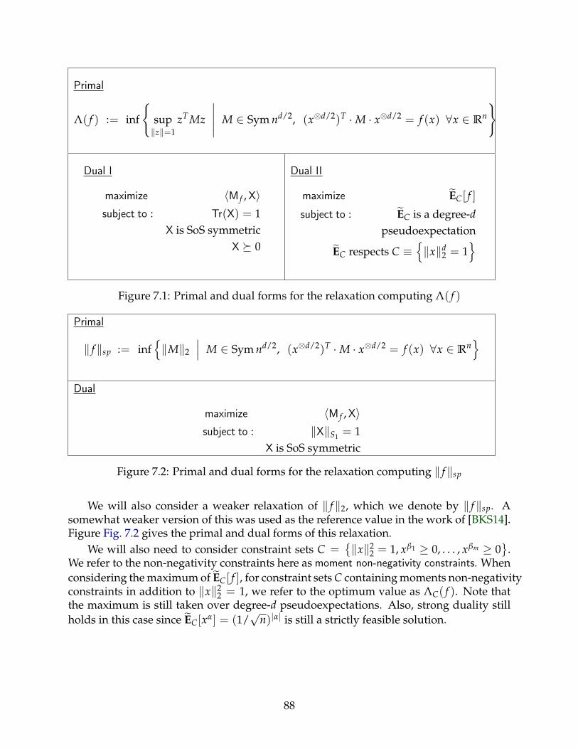
Primal
Λ( f ) := inf
sup‖z‖=1
zT Mz
∣∣∣∣∣ M ∈ Sym nd/2, (x⊗d/2)T ·M · x⊗d/2 = f (x) ∀x ∈ Rn
Dual I
maximize 〈M f ,X〉subject to : Tr(X) = 1
X is SoS symmetricX 0
Dual II
maximize EC[ f ]
subject to : EC is a degree-dpseudoexpectation
EC respects C ≡‖x‖d
2 = 1
Figure 7.1: Primal and dual forms for the relaxation computing Λ( f )
Primal
‖ f ‖sp := inf‖M‖2
∣∣∣ M ∈ Sym nd/2, (x⊗d/2)T ·M · x⊗d/2 = f (x) ∀x ∈ Rn
Dual
maximize 〈M f ,X〉subject to : ‖X‖S1 = 1
X is SoS symmetric
Figure 7.2: Primal and dual forms for the relaxation computing ‖ f ‖sp
We will also consider a weaker relaxation of ‖ f ‖2, which we denote by ‖ f ‖sp. Asomewhat weaker version of this was used as the reference value in the work of [BKS14].Figure Fig. 7.2 gives the primal and dual forms of this relaxation.
We will also need to consider constraint sets C =‖x‖2
2 = 1, xβ1 ≥ 0, . . . , xβm ≥ 0
.We refer to the non-negativity constraints here as moment non-negativity constraints. Whenconsidering the maximum of EC[ f ], for constraint sets C containing moments non-negativityconstraints in addition to ‖x‖2
2 = 1, we refer to the optimum value as ΛC( f ). Note thatthe maximum is still taken over degree-d pseudoexpectations. Also, strong duality stillholds in this case since EC[xα] = (1/
√n)|α| is still a strictly feasible solution.
88
7.4.1 Properties of relaxations obtained from constrained pseudoexpec-tations
We use the following claim, which is an easy consequence of the fact that the sum-of-squares algorithm can produce a certificate of optimality (see [OZ13]). In particular,if maxEC
EC[ f ] = ΛC( f ) for a degree-q1 pseudoexpectation operator respecting C con-taining ‖x‖2
2 = 1 and moment non-negativity constraints for β1, . . . , βm, then for everyλ > ΛC( f ), we have that λ− f can be certified to be positive by showing that λ− f ∈ Σq1
C .
Here Σ(q1)C is the set of all expressions of the form
λ− f = ∑j
pj ·(‖x‖2
2 − 1)+ ∑
S⊆[m]
hS(x) ·∏i∈S
xβi ,
where each hS is a sum of squares of polynomials and the degree of each term is at mostq1.
Lemma 7.4.2. Let ΛC( f ) denote the maximum of EC[ f ] over all degree-d pseudoexpectationoperators respecting C. Then, for a pseudoexpectation operator of degree d′ (respecting C) anda polynomial p of degree at most (d′ − d)/2, we have that
EC
[p2 · f
]≤ EC
[p2]·ΛC( f ) .
Proof. As described above, for any λ > ΛC( f ), we can write λ− f = g for g ∈ Σ(d)C . Since
the degree of each term in p2 · g is at most d′, we have by the properties of pseudoexpec-tation operators (of degree d′) that
λ · EC
[p2]− EC
[p2 · f )
]= EC
[p2 · (λ− f )
]= EC
[p2 · g
]≥ 0 .
The following monotonicity claim for non-negative coefficient polynomials will comein handy in later sections.
Lemma 7.4.3. Let C be a system of polynomial constraints containing ∀β ∈ Nnt , xβ ≥ 0.
Then for any non-negative coefficient polynomials f and g of degree t, and such that f ≥ g(coefficient-wise, i.e. f − g has non-negative coefficients), we have ΛC( f ) ≥ ΛC(g).
Proof. For any pseudo-expectation operator EC respecting C, we have EC[ f − g] ≥ 0 be-cause of the moment non-negativity constraints and by linearity.
So let EC be a pseudo-expectation operator realizing ΛC(g). Then we have,
ΛC( f ) ≥ EC[ f ] = EC[g] + EC[ f − g] = ΛC(g) + EC[ f − g] ≥ 0.
89
Chapter 8
Worst Case Polynomial Optimizationover the Sphere
In this chapter, we study the problem of optimizing homogeneous polynomials over theunit sphere. Formally, given an n-variate degree-d homogeneous polynomial f , the goalis to compute
‖ f ‖2 := sup‖x‖=1
| f (x)| . (8.1)
We develop general techniques to design and analyze algorithms for polynomial opti-mization over the sphere. The sphere constraint is one of the simplest constraints forpolynomial optimization and thus is a good testbed for techniques. Indeed, we believethese techniques will also be useful in understanding polynomial optimization for otherconstrained settings.
8.1 Algorithmic Results
The following result shows that Λ(
f q/d)d/qapproximates ‖ f ‖2 within polynomial fac-
tors, and also gives an algorithm to approximate ‖ f ‖2 with respect to the upper boundΛ(
f q/d)d/q. In the statements below and the rest of this section, Od(·) and Ωd(·) notations
hide 2O(d) factors. Our algorithmic results are as follows:
Theorem 8.1.1. Let f be an n-variate homogeneous polynomial of degree-d, and let q ≤ n be aninteger divisible by 2d. Then,
Arbitrary f :(
Λ(
f q/d))d/q
≤ Od
((n/q)d/2−1
)· ‖ f ‖2
f with Non-neg. Coefficients:(
ΛC
(f q/d
))d/q≤ Od
((n/q)d/4−1/2
)· ‖ f ‖2
f with Sparsity m:(
Λ(
f q/d))d/q
≤ Od
(√m/q
)· ‖ f ‖2.
(where ΛC(·) is a a related efficiently computable quantity that we define in Section 7.4)
90
Furthermore, there is a deterministic algorithm that runs in nO(q) time and returns x suchthat
| f (x)| ≥Λ(
f q/d)d/q
Od(c(n, d, q))
where c(n, d, q) is (n/q)d/2−1, (n/q)d/4−1/2 and√
m/q respectively, for each of the above cases(the inequality uses ΛC(·) in the case of polynomials with non-negative coefficients).
Remark 8.1.2. Interestingly, our deterministic algorithms only involve computing the maxi-mum eigenvectors of nO(q) different matrices in IRn×n, and actually don’t require computingΛ(
f q/d)d/q (even though this quantity can also be computed in nO(q) time by the sum-of-squares
SDP; see Section 8.2). The quantity Λ(
f q/d)d/q is only used in the analysis.
Remark 8.1.3. If m = n ρ·d for ρ < 1/3, then for all q ≤ n1−ρ, the√
m/q-approximation forsparse polynomials is better than the (n/q)d/2−1 arbitrary polynomial approximation.
Remark 8.1.4. In cases where ‖ f ‖2 = fmax (such as when d is odd or f has non-negative coeffi-cients), the above result holds whenever q is even and divisible by d, instead of 2d.
A key technical ingredient en route establishing the above results is a method to re-duce the problem for arbitrary polynomials to a list of multilinear polynomial problems(over the same variable set). We believe this to be of independent interest, and describeits context and abstract its consequence (Theorem 8.1.5) next.
Let Mg be a matrix representation of a degree-q homogeneous polynomial g, and letK = (I, J) ∈ [n]q/2 × [n]q/2 have all distinct elements. Observe that there are q! distinctentries of Mg including K across which, one can arbitrarily assign values and maintainthe property of representing g, as long as the sum across all q! entries remains the same(specifically, this is the set of all permutations of K). In general for K′ = (I′, J′) ∈ [n]q/2 ×[n]q/2, we define the orbit of K′ denoted by O(K′), as the set of permutations of K′, i.e. thenumber of entries to which ’mass’ from Mg[I′, J′] can be moved while still representing g.
As q increases, the orbit sizes of the entries increase, and to show better bounds onΛ(
f q/d), one must exploit these additional "degrees of freedom" in representations off q/d. However, a big obstacle is that the orbit sizes of different entries can range anywherefrom 1 to q!, two extremal examples being ((1, . . . 1), (1, . . . 1)) and ((1, . . . q/2), (q/2 +1, . . . q)). This makes it hard to exploit the additional freedom afforded by growing q.Observe that if g were multilinear, all matrix entries corresponding to non-zero coeffi-cients have a span of q! and indeed it turns out to be easier to analyze the approxima-tion factor in the multilinear case as a function of q since the representations of g can behighly symmetrized. However, we are still faced with the problem of f q/d being highlynon-multilinear. The natural symmetrization strategies that work well for multilinearpolynomials fail on general polynomials, which motivates the following result:
Theorem 8.1.5 (Informal version of Theorem 8.7.13). For even q, let g(x) be a degree-q homo-geneous polynomial. Then there exist multilinear polynomials g1(x), . . . , gm(x) of degree at mostq, such that
Λ(g)‖g‖2
≤ 2O(q) ·maxi∈[m]
Λ(gi)
‖gi‖2
91
By combining Theorem 8.1.5 (or an appropriate generalization) with the appropriateanalysis of the multilinear polynomials induced by f q/d, we obtain the aforementionedresults for various classes of polynomials.
Weak decoupling lemmas. A common approach for reducing to the multilinear caseis through more general “decoupling” or “polarization” lemmas (see e.g., Lemma 8.7.6),which also have variety of applications in functional analysis and probability [DlPG12].However, such methods increase the number of variables to nq, which would completelynullify any advantage obtained from the increased degrees of freedom.
Our proof of Theorem 8.1.5 (and its generalizations) requires only a decoupling withsomewhat weaker properties than given by the above lemmas. However, we need it to bevery efficient in the number of variables. In analogy with “weak regularity lemmas” incombinatorics, which trade structural control for complexity of the approximating object,we call these results “weak decoupling lemmas” (see Section 8.6.1 and Lemma 8.7.12).They provide a milder form of decoupling but only increase the number of variables to2n (independently of q).
We believe these could be more generally applicable; in particular to other constrainedsettings of polynomial optimization as well as in the design of sub-exponential algo-rithms. Our techniques might also be able to yield a full tradeoff between the numberof variables and quality of decoupling.
8.2 Connection to Sum-of-Squares hierarchy
The Sum of Squares Hierarchy (SoS) is one of the the most canonical and well-studied ap-proaches to attack polynomial optimization problems. Algorithms based on this frame-work are parameterized by the degree or level q of the SoS relaxation. For the case of op-timization of a homogenous polynomial h of even degree q (with some matrix representa-tion Mh) over the unit sphere, the level q SoS relaxes the non-convex program of maximiz-ing (x⊗q/2)T ·Mh · x⊗q/2 = h(x) over x ∈ Rn with ‖x‖2 = 1, to the semidefinite programof maximizing Tr
(MT
h X)
over all positive semidefinite matrices X ∈ R[n]q/2×[n]q/2with
Tr(X) = 1. (This is a relaxation because X = x⊗q/2(x⊗q/2)T is psd with Tr(X) = ‖x‖q2.)
It is well known (see for instance [Lau09]) that the quantity Λ(h) from Eq. (7.1) is thedual value of this SoS relaxation. Further, strong duality holds for the case of optimiza-tion on the sphere and therefore Λ(h) equals the optimum of the SoS SDP and can becomputed in time nO(q). (See Section 7.3 for more detailed SoS preliminaries.) In lightof this, our results from Theorem 8.1.1 can also be viewed as a convergence analysis ofthe SoS hierarchy for optimization over the sphere, as a function of the number of levelsq. Such results are of significant interest in the optimization community, and have beenstudied for example in [DW12, dKLS14] (see Section 8.3 for a comparison of results).
SoS Lower Bounds. While the approximation factors in our upper bounds of Theo-rem 8.1.1 are modest, there is evidence to suggest that this is inherent.
92
When h is a degree-q polynomial with random i.i.d ±1 coefficients, we will show in
Chapter 9 that there is a constant c such that w.h.p.(
nqc+o(1)
)q/4≤ Λ(h) ≤
(n
qc−o(1)
)q/4. On
the other hand, ‖h‖2 ≤ O(√
nq log q) w.h.p. Thus the ratio between Λ(h) and ‖h‖2 canbe as large as Ωq(nq/4−1/2).
Hopkins et al. [HKP+17] recently proved that degree-d polynomials with randomcoefficients achieve a degree-q SoS gap of roughly (n/qO(1))d/4−1/2 (provided q > nε forsome constant ε > 0). This is also a lower bound on the ratio between Λ
(f q/d)d/q
and‖ f ‖2 for the case of arbitrary polynomials. Note that this lower bound is roughly squareroot of our upper bound from Theorem 8.1.1. Curiously, our upper bound for the caseof polynomials with non-negative coefficients essentially matches this lower bound forrandom polynomials.
Non-Negative Coefficient Polynomials. In this chapter, we give a new lower boundconstruction for the case of non-negative polynomials, To the best of out knowledge, theonly previous lower bound for this problem, was known through Nesterov’s reduction[DK08], which only rules out a PTAS. We give the following polynomially large lowerbound. The gap applies for random polynomials associated with a novel distribution of4-uniform hypergraphs, and is analyzed using subgraph counts in a random graph.
Theorem 8.2.1. There exists an n variate degree-4 homogeneous polynomial f with non-negativecoefficients such that
‖ f ‖2 ≤ (log n)O(1) and Λ( f ) ≥ Ω(n1/6) .
For larger degree t, we prove an nΩ(t) gap between ‖h‖2 and a quantity ‖h‖sp that isclosely related to Λ(h). Specifically, ‖h‖sp is defined by replacing the largest eigenvalueof matrix representations Mh of h in Eq. (7.1) by the spectral norm ‖Mh‖2. (See Fig. 7.2 fora formal definition.) Note that ‖h‖sp ≥ maxΛ(h) , Λ(−h). Like Λ(·), ‖ · ‖sp suggestsa natural hierarchy of relaxations for the problem of approximating ‖h‖2, obtained bycomputing ‖hq/t‖t/q
sp as the q-th level of the hierarchy.
We prove a lower bound of nq/24/ (q · log n)O(q) on ‖ f q/4‖sp where f is as in Sec-tion 8.9. This not only gives ‖ · ‖sp gaps for the degree-q optimization problem on polyno-mials with non-negative coefficients, but also an n1/6/(q log n)O(1) gap on higher levelsof the aforementioned ‖ · ‖sp hierarchy for optimizing degree-4 polynomials with non-negative coefficients. Formally we show:
Theorem 8.2.2. Let g := f q/4 where f is the degree-4 polynomial as in Section 8.9. Then
‖g‖sp
‖g‖2≥ nq/24
(q log n)O(q).
Our lower bound on ‖ f q/4‖sp is based on a general tool that allows one to “lift” level-4 ‖ · ‖sp gaps, that meet one additional condition, to higher levels. While we derive finalresults only for the weaker relaxation ‖ · ‖sp, the underlying structural result may prove
93
useful in lifting SoS lower bounds (i.e. gaps for Λ(·)) as well. Recently, the insightfulpseudo-calibration approach [BHK+16] has provided a recipe to give higher level SoSlower bounds for certain average-case problems. We believe our lifting result might simi-larly be useful in the context of worst-case problems, where in order to get higher degreelower bounds, it suffices to give lower bounds for constant degree SoS with some addi-tional structural properties.
8.3 Related Work
Polynomial optimization is a vast area with several previous results. Below, we collect theresults most relevant for comparison with the ones in this chapter, grouped by the classof polynomials. Please see the excellent monographs [Lau09, Las09] for a survey.
Arbitrary Polynomials. For general homogeneous polynomials of degree-d, an Od(nd/2−1)
approximation was given by He et al. [HLZ10], which was improved to Od((n/ log n)d/2−1)
by So [So11]. The convergence of SDP hierarchies for polynomial optimization over thesphere was analyzed by Faybusovich [Fay04] and Doherty and Wehner [DW12] and sub-sequent to the publication of our work by deKlerk and Laurent [dKL19]. However, forq n levels, these convergence results would only imply a weaker bound of (O(n)/q)d/2.
Thus, our results can be seen as giving a stronger interpolation between the poly-nomial time algorithms obtained by [HLZ10, So11] and the exponential time algorithmsgiven by Ω(n) levels of SoS, although the bounds obtained by [Fay04, DW12, dKL19] aretighter (by a factor of 2O(d)) for q = Ω(n) levels.
For the case of arbitrary polynomials, we believe a tradeoff between running time andapproximation quality similar to ours can also be obtained by considering the tradeoffsfor the results of Brieden et al. [BGK+01] used by So [So11]. However, to the best ofour knowledge, this is not published. In particular, So uses the techniques of Khot andNaor [KN08] to reduce degree-d polynomial optimization to d− 2 instances of the prob-lem of optimizing the `2 diameter of a convex body. This is solved by [BGK+01], whogive an O((n/k)1/2) approximation in time 2k · nO(1). We believe this can be combinedwith proof of So, to yield a Od
((n/q)d/2−1) approximation in time 2q. We note here that
the method of Khot and Naor [KN08] cannot be improved further (up to polylog) for thecase d = 3 (see Section 8.12). Our results for the case of arbitrary polynomials show thatsimilar bounds can also be obtained by a very generic algorithm given by the SoS hier-archy. Moreover, the general techniques developed here are versatile and demonstrablyapplicable to various other cases (like polynomials with non-negative coefficients, sparsepolynomials, worst-case sparse PCA) where no alternate proofs are available. The tech-niques of [KN08, So11] are oblivious to the structure in the polynomials and it appears tobe unlikely that similar results can be obtained by using diameter estimation techniques.
Polynomials with Non-negative Coefficients. The case of polynomials with non-negativecoefficients was considered by Barak, Kelner, and Steurer [BKS14] who proved that therelaxation obtained by Ω(d3 · log n/ε2) levels of the SoS hierarchy provides an ε · ‖ f ‖BKSadditive approximation to the quantity ‖ f ‖2. Here, the parameter we denote by ‖ f ‖BKS
94
corresponds to a relaxation for ‖ f ‖2 that is weaker than the one given by ‖ f ‖sp.1 Their re-sults can be phrased as showing that a relaxation obtained by q levels of the SoS hierarchygives an approximation ratio of
1 +(
d3 · log nq
)1/2
· ‖ f ‖BKS
‖ f ‖2.
Motivated by connections to quantum information theory, they were interested in thespecial case where ‖ f ‖BKS/‖ f ‖2 is bounded by a constant. However, this result does notimply strong multiplicative approximations outside of this special case since in general‖ f ‖BKS and ‖ f ‖2 can be far apart. In particular, we are able to establish that there existpolynomials f with non-neg. coefficients such that ‖ f ‖BKS/‖ f ‖2 ≥ nd/24. Moreover weconjecture that the worst-case gap between ‖ f ‖BKS and ‖ f ‖2 for polynomials with non-neg. coefficients is as large as Ωd((n/d)d/4−1/2) (note that the conjectured (n/d)d/4−1/2
gap for non-negative coefficient polynomials is realizable using arbitrary polynomials,i.e. we show in Chapter 9 that polynomials with i.i.d. ±1 coefficients achieve this gapw.h.p.).
Our results show that q levels of SOS gives an (n/q)d/4−1/2 approximation to ‖ f ‖2which has a better dependence on q and consequently, converges to a constant factorapproximation after Ω(n) levels.
2-to-4 norm. It was proved in [BKS14] that for any matrix A, q levels of the SoS hierarchyapproximates ‖A‖4
2→4 within a factor of
1 +(
log nq
)1/2
· ‖A‖22→2‖A‖2
2→∞
‖A‖42→4
.
Brandao and Harrow [BH15] also gave a nets based algorithm with runtime 2q that achievesthe same approximation as above. Here again, the cases of interest were those matricesfor which ‖A‖2
2→2‖A‖22→∞ and ‖A‖4
2→4 are at most constant apart.We would like to bring attention to an open problem in this line of work. It is not hard
to show that for an m × n matrix A with i.i.d. Gaussian entries, ‖A‖22→2 = Θ(m + n),
‖A‖22→∞ = Θ(n), and ‖A‖2
2→4 = Θ(m + n2) which implies the worst case approximationfactor achieved above is Ω(n/
√q) when we take m = Ω(n2).
Our result for arbitrary polynomials of degree-4, achieves an approximation factor ofO(n/q) after q levels of SoS which implies that the current best known approximation2-to-4 norm is oblivious to the structure of the 2-to-4 polynomial and seems to suggestthat this problem can be better understood for arbitrary tall matrices. For instance, canone get a
√m/q approximation for (m × n) matrices (note that [BH15] already implies
a√
m/q-approximation for all m, and our result implies a√
m/q-approximation whenm = Ω(n2)).
Random Polynomials. For the case when f is a degree-d homogeneous polynomialwith i.i.d. random ±1 coefficients the concurrent works [BGL16, RRS16] showed that
1Specifically, ‖ f ‖BKS minimizes the spectral norm over a smaller set of matrix representations of f than‖ f ‖sp which allows all matrix representations.
95
degree-q SoS certifies an upper bound on ‖ f ‖2 that is with high probability at mostO((n/q)d/4−1/2) · ‖ f ‖2. Curiously, this matches our approximation guarantee for the caseof arbitrary polynomials with non-negative coefficients. This problem was also studied forthe case of sparse random polynomials in [RRS16] motivated by applications to refutingrandom CSPs.
8.4 Organization
We cover some preliminaries in Section 8.5 and provide an overview of our proofs andtechniques in Section 8.6. Chapter 7 provides details of various relaxations used in thisdocument, and their duals in terms of the Sum-of-Squares hierarchy. We first give a ba-sic version of the reduction from general to multilinear polynomials in Section 8.7, whichonly obtains a weaker result (without the additive term in the exponent). Section 8.8 givesa generalization of this reduction, which yields Theorem 8.1.1. We prove an SoS lowerbound for degree-4 polynomials with non-negative coefficients in Section 8.9. In Sec-tion 8.10, we provide a general technique for lifting lower bounds for the slightly weakerrelaxation given by ‖ f ‖sp, to relaxation higher level relaxations.
8.5 Preliminaries and Notation
Definition 8.5.1 (Folded Polynomials). A degree-(d1, d2) folded polynomial f ∈(Rd2[x]
)d1[x]
is defined to be a polynomial of the form
f (x) = ∑α∈Nn
d1
f α(x) · xα ,
where each f α(x) ∈ Rd2 [x] is a homogeneous polynomial of degree d2. Folded polynomials overR+ are defined analogously.
- We refer to the polynomials f α as the folds of f and the terms xα as the monomials in f .
- A folded polynomial can also be used to define a degree d1 + d2 polynomial by multiplyingthe monomials with the folds (as polynomials in R[x]). We refer to this polynomial inRd1+d2 [x] as the unfolding of f , and denote it by U( f ).
- For a degree (d1, d2)-folded polynomial f and r ∈N, we take f r to be a degree-(r · d1, r · d2)folded polynomial, obtained by multiplying the folds as coefficients.
An additional operation on folded polynomials. We define the following operation(and it’s folded counterpart) which in the case of a multilinear polynomial corresponds(up to scaling) to the sum of a row of the SoS-symmetric matrix representation of thepolynomial. This will be useful in our result for non-negative polynomials.
96
Definition 8.5.2 (Collapse). Let f ∈ Rd[x] be a polynomial. The k-collapse of f , denoted asCk( f ) is the degree d− k polynomial g given by,
g(x) = ∑γ∈Nn
d−k
gγ · xγ where gγ = ∑α∈Nn
k
fγ+α .
For a degree-(d1, d2) folded polynomial f , we define Ck( f ) similarly as the degree-(d1 − k, d2)folded polynomial g given by,
g(x) = ∑γ∈Nn
d1−k
gγ(x) · xγ where gγ = ∑α∈Nn
k
f γ+α .
8.6 Overview of Proofs and Techniques
In the interest of clarity, we shall present all techniques for the special case where f is anarbitrary degree-4 homogeneous polynomial. We shall further assume that ‖ f ‖2 = fmaxjust so that Λ( f ) is a relaxation of ‖ f ‖2. Summarily, the goal of this section is to give anoverview of an O(n/q)-approximation of ‖ f ‖2, i.e.
Λ(
f q/4)4/q
≤ O(n/q) · ‖ f ‖2.
Many of the high level ideas remain the same when considering higher degree polynomi-als and special classes like polynomials with non-negative coefficients, or sparse polyno-mials.
8.6.1 Warmup: (n2/q2)-Approximation
We begin with seeing how to analyze constant levels of the Λ(·) relaxation and will thenmove onto higher levels in the next section. The level-4 relaxation actually achieves an n-approximation, however we will start with n2 as a warmup and cover the n-approximationa few sections later.
n2-Approximation using level-4 relaxation
We shall establish that Λ( f ) ≤ O(n2) · ‖ f ‖2. Let M f be the SoS-symmetric representationof f , let xi1 xi2 xi3 xi4 be the monomial whose coefficient in f has the maximum magnitude,and let B be the magnitude of this coefficient. Now by Gershgorin circle theorem, wehave Λ( f ) ≤ ‖M f ‖2 ≤ n2 · B.
It remains to establish ‖ f ‖2 = Ω(B). To this end, define the decoupled polynomialF (x, y, z, t) := (x⊗ y)T ·M f · (z⊗ t) and define the decoupled two-norm as
‖F‖2 := sup‖x‖,‖y‖,‖z‖,‖t‖=1
F (x, y, z, t).
97
It is well known that ‖ f ‖2 = Θ(‖F‖2) (see Lemma 8.6.1). Thus, we have,
‖ f ‖2 = Ω(‖F‖2) ≥ Ω(|F (ei1 , ei2 , ei3 , ei4)|
)= Ω(B) = Ω
(Λ( f ) /n2
).
In order to better analyze Λ(
f q/4)4/qwe will need to introduce some new techniques.
(n2/q2)-Approximation Assuming Theorem 8.1.5
We will next show that Λ(
f q/4)4/q ≤ O(n2/q2) · ‖ f ‖2 (for q divisible by 4). In fact, one canshow something stronger, namely that for every homogeneous polynomial g of degree-q, Λ(g) ≤ 2O(q) · (n/q)q/2 · ‖g‖2 which clearly implies the above claim (also note thatfor the target O(n2/q2)-approximation to ‖ f ‖2, losses of 2O(q) in the estimate of ‖g‖2 arenegligible, while factors of the order qΩ(q) are crucial).
Given the additional freedom in choice of representation (due to the polynomial hav-ing higher degree), a first instinct would be to completely symmetrize, i.e. take theSoS-symmetric representation of g, and indeed this works for multilinear g (see Theo-rem 8.7.16 for details).
However, the above approach of taking the SoS-symmetric representation breaksdown when the polynomial is non-multilinear. To circumvent this issue, we employ The-orem 8.1.5 which on combining with the aforementioned multilinear polynomial result,yields that for every homogeneous polynomial g of degree-q, Λ(g) ≤ (n/q)q/2 · ‖g‖2. Theproofs of Theorem 8.1.5 and it’s generalizations (that will be required for the n/q approx-imation), are quite non-trivial and are the most technically involved sections of our upperbound results. We shall next give an outline of the proof of Theorem 8.1.5.
Reduction to Optimization of Multi-linear Polynomials
One of the main techniques we develop in this work, is a way of reducing the optimiza-tion problem for general polynomials to that of multi-linear polynomials, which does notincrease the number of variables. While general techniques for reduction to the multi-linearcase have been widely used in the literature [KN08, HLZ10, So11] (known commonlyas decoupling/polarization techniques), these reduce the problem to optimizing a multi-linear polynomial in n · d variables (when the given polynomial h is of degree d). Belowis one example:
Lemma 8.6.1 ([HLZ10]). Let A be a SoS-symmetric d-tensor and let h(x) := 〈A, x⊗d〉. Then‖h‖2 ≥ 2−O(d) ·max‖xi‖=1〈A, x1 ⊗ · · · ⊗ xd〉.
Since we are interested in the improvement in approximation obtained by consideringf q/4 for a large q, applying these would yield a multi-linear polynomial in n · q variables.For our analysis, this increase in variables exactly cancels the advantage we obtain byconsidering f q/4 instead of f (i.e., the advantage obtained by using q levels of the SoShierarchy).
98
We can uniquely represent a homogeneous polynomial g of degree q as
g(x) = ∑|α|≤q/2
x2α · G2α(x) =q/2
∑r=0
∑|α|=r
x2α · G2α(x) =q/2
∑r=0
gr(x) , (8.2)
where each G2α is a multi-linear polynomial and gr(x) := ∑|α|=r x2α · G2α(x). We reducethe problem to optimizing ‖G2α‖2 for each of the polynomials G2α. More formally, weshow that
Λ(g)‖g‖2
≤ maxα∈Nn
≤q/2
Λ(G2α)
‖G2α‖2· 2O(q) (8.3)
As a simple and immediate example of its applicability, Eq. (8.3) provides a simple proofof a polytime constant factor approximation for optimization over the simplex (actuallythis case is known to admit a PTAS [dKLP06, dKLS15]). Indeed, observe that a simplexoptimization problem for a degree-q/2 polynomial in the variable vector y can be reducedto a sphere optimization by substituting yi = x2
i . Now since every variable present ina monomial has even degree in that monomial, each G2α is constant, which implies aconstant factor approximation (dependent on q) on applying Eq. (8.3).
Returning to our overview of the proof, note that given representations of each ofthe polynomials G2α, each of the polynomials gr can be represented as a block-diagonalmatrix with one block corresponding to each α. Combining this with triangle inequal-ity and the fact that the maximum eigenvalue of a block-diagonal matrix is equal to themaximum eigenvalue of one of the blocks, gives the following inequality:
Λ(g) ≤ (1 + q/2) · maxα∈Nn
≤q/2
Λ(G2α) . (8.4)
We can further strengthen Eq. (8.4) by averaging the "best" representation of G2α over|O(α)| diagonal-blocks which all correspond to x2α. This is the content of Lemma 8.7.2wherein we show
Λ(g) ≤ (1 + q/2) · maxα∈Nn
≤q/2
Λ(G2α)
|O(α)| . (8.5)
Since |O(α)| can be as large as qΩ(q), the above strengthening is crucial. We then provethe following inequality, which shows that the decomposition in Eq. (8.2) not only gives ablock-diagonal decomposition for matrix representations of g, but can in fact be thoughtof as a “block-decomposition” of the tensor corresponding to g (with regards to comput-ing ‖g‖2). Just as the maximum eigenvalue of a block-diagonal matrix is at least themaximum eigenvalue of a block, we show that
‖g‖2 ≥ 2−O(q) · maxα∈Nn
≤q/2
‖G2α‖2
|O(α)| . (8.6)
The above inequality together with Eq. (8.5), implies Eq. (8.3).
99
Bounding ‖g‖2 via a new weak decoupling lemma
Recall that the expansion of g(x) in Eq. (8.2), contains the term x2α · G2α(x). The key partof proving the bound in Eq. (8.6) is to show the following “weak decoupling” result forx2α and G2α.
∀α ‖g‖2 ≥ max‖y‖=‖x‖=1
y2α · G2α(x) · 2−O(q) = max‖y‖=1
y2α · ‖G2α‖2 · 2−O(q).
The proof of Eq. (8.6) can then be completed by considering the unit vector y :=√
α/√|α|, i.e. y := ∑i∈[n]
√αi√|α|· ei. A careful calculation shows that y2α ≥ 2−O(q)/ |O(α)|
which finishes the proof.The primary difficulty in establishing the above decoupling is the possibility of can-
cellations. To see this, let x∗ be the vector realizing ‖G2α‖2 and substitute z = (x∗+ y) intog. Clearly, y2α · G2α(x∗) is a term in the expansion of g(z), however there is no guaranteethat the other terms in the expansion don’t cancel out this value. To fix this our proofrelies on multiple delicate applications of the first-moment method, i.e. we consider acomplex vector random variable Z(x∗, y) that is a function of x∗ and y, and argue aboutE[|g(Z)|].The base case of α = 0n. We first consider the base case with α = 0n, where we definey2α = 1. This amounts to showing that for every homogeneous polynomial h of degree t,‖h‖2 ≥ ‖hm‖2 · 2−O(t) where hm is the restriction of h to it’s multilinear monomials.
Given the optimizer x∗ of ‖hm‖2, let z be a random vector such that each Zi = x∗i withprobability p and Zi = 0 otherwise. Then, E[h(Z)] is a univariate degree-t polynomialin p with the coefficient of pt equal to hm(x∗). An application of Chebyshev’s extremalpolynomial inequality (Lemma 8.7.5) then gives that there exists a value of the probabilityp such that
‖h‖2 ≥ E [|h(Z)|] ≥ |E [h(Z)]| ≥ 2−O(t) · |hm(x∗)| = 2−O(t) · ‖hm‖2 .
For the case of general α, we first pass to the complex version of ‖g‖2 defined as
‖g‖c2 := sup
z∈Cn,‖z‖=1|g(z)| .
We use another averaging argument together with an application of the polarizationlemma (Lemma 8.6.1) to show that we do not loose much by considering ‖g‖c
2. In partic-ular, ‖g‖2 ≤ ‖g‖c
2 ≤ 2O(q) · ‖g‖2.
The case of g = gr. In this case, the problem reduces to showing that for all α ∈ Nnr and
for all y ∈ Sn−1,‖gr‖c
2 ≥ y2α · ‖G2α‖2 · 2−O(q).
Fix any α ∈ Nnr , and let ω ∈ Cn be a complex vector random variable, such that ωi is
an independent and uniformly random (2αi + 1)-th root of unity. Let Ξ be a random(q− 2r + 1)-th root of unity, and let x∗ be the optimizer of ‖G2α‖2. Let Z := ω y + Ξ · x∗,
100
where ω y denotes the coordinate-wise product. Observe that for any α′, γ such that|α′| = r, |γ| = q− 2r, γ ≤ 1,
E
[∏
iωi · Ξ · Z2α′+γ
]=
y2α · (x∗)γ if α′ = α
0 otherwise
By linearity, this implies E[∏i ωi · Ξ · gr(Z)] = y2α · G2α(x∗). The claim then follows bynoting that
‖gr‖c2 ≥ E [|gr(Z)|] = E
[∣∣∣∣∣∏iωi · Ξ · gr(Z)
∣∣∣∣∣]≥∣∣∣∣∣E
[∏
iωi · Ξ · gr(Z)
]∣∣∣∣∣ ≥ y2α · ‖G2α‖2.
The general case. The two special cases considered here correspond to the cases whenwe need to extract a specific gr (for r = 0), and when we need to extract a fixed α from agiven gr. The argument for the general case uses a combination of the arguments for boththese cases. Moreover, to get an O(n/q) approximation, we also need versions of suchdecoupling lemmas for folded polynomials to take advantage of “easy substructures” asdescribed next.
8.6.2 Exploiting Easy Substructures via Folding and Improved Approx-imations
To obtain the desired n/q-approximation to ‖ f ‖2, we need to use the fact that the problemof optimizing quadratic polynomials can be solved in polynomial time, and moreoverthat SoS captures this. More generally, in this section we consider the problem of gettingimproved approximations when a polynomial contains "easy substructures". It is not hardto obtain improved guarantees when considering constant levels of SoS. The second maintechnical contribution of our work is in giving sufficient conditions under which higherlevels of SoS improve on the approximation of constant levels of SoS, when consideringthe optimization problem over polynomials containing "easy substructures".
As a warmup, we shall begin with seeing how to exploit easy substructures at con-stant levels by considering the example of degree-4 polynomials that trivially "contain"quadratics.
n-Approximation using Degree-4 SoS
Given a degree-4 homogeneous polynomial f (assume f is multilinear for simplicity), weconsider a degree-(2, 2) folded polynomial h, whose unfolding yields f , chosen so thatmax‖y‖=1 ‖h(y)‖2 = Θ(‖ f ‖2) (recall that an evaluation of a folded polynomial returns apolynomial, i.e., for a fixed y, h(y) is a quadratic polynomial in the indeterminate x). Suchan h always exists and is not hard to find based on the SoS-symmetric representation off . Also recall,
h(x) = ∑|β|=2, β≤1
hβ(x) · xβ ,
101
where each hβ is a quadratic polynomial (the aforementioned phrase "easy substructures"is referencing the folds: hβ which are easy to optimize). Now by assumption we have,
‖ f ‖2 ≥ max|β|=2, β≤1
‖h(β/√
2)‖2 = max|β|=2, β≤1
‖hβ‖2/2.
We then apply the block-matrix generalization of Gershgorin circle theorem to the SoS-symmetric matrix representation of f to show that
Λ( f ) ≤ ‖ f ‖sp ≤ n · max|β|=2, β≤1
‖hβ‖sp = n · max|β|=2, β≤1
‖hβ‖2 ,
where the last step uses the fact that hβ is a quadratic, and ‖ · ‖sp is a tight relaxation of‖ · ‖2 for quadratics. This yields the desired n-approximation.
n/q-approximation using Degree-q SoS
Following the cue of the n2/q2-approximation, we derive the desired n/q bound by prov-ing a folded-polynomial analogue of every claim in the previous section (including themultilinear reduction tools), a notable difference being that when we consider a powerf q/4 of f , we need to consider degree-(q− 2q/4, 2q/4) folded polynomials, since we wantto use the fact that any product of q/4 quadratic polynomials is “easy” for SoS (in con-trast to Section 8.6.2 where we only used the fact quadratic polynomials are easy for SoS).We now state an abstraction of the general approach we use to leverage the tractability ofthe folds.
Conditions for Exploiting "Easy Substructures" at Higher Levels of SoS. Let d := d1 + d2and f := U(h) where h is a degree-(d1, d2) folded polynomial that satisfies
sup‖y‖=1
‖h(y)‖2 = Θd(‖ f ‖2) .
Implicit in Section 8.8, is the following theorem we believe to be of independent interest:
Theorem 8.6.2. Let h, f be as above, and let
Γ := min
Λ(p)‖p‖2
∣∣∣ p(x) ∈ span(
hβ
∣∣∣ β ∈Nnd2
).
Then for any q divisible by 2d, Λ(
f q/d)d/q ≤ Od(Γ · (n/q)d1/2) · ‖ f ‖2.
In other words, if degree-d2 SoS gives a good approximation for every polynomialin the subspace spanned by the folds of h, then higher levels of SoS give an improvingapproximation that exploits this. In this work, we only apply the above with Γ = 1, whereexact optimization is easy for the space spanned by the folds.
While we focus on general polynomials for the overview, let us remark that in the caseof polynomials with non-negative coefficients, the approximation factor in Theorem 8.6.2becomes Od
(δ · (n/q)d1/4).
102
8.6.3 Lower Bounds for Polynomials with Non-negative Coefficients
Degree-4 Lower Bound for Polynomials with Non-Negative Coefficients
We discuss some of the important ideas from the proof of Section 8.9. The lower boundin Chapter 9 proves Λ( f )
‖ f ‖2is large by considering a random polynomial f where each co-
efficient of f is an independent (Gaussian) random variable with bounded variance. Themost natural adaptation of the above strategy to degree-4 polynomials with non-negativecoefficients is to consider a random polynomial f where each coefficient fα is indepen-dently sampled such that fα = 1 with probability p and fα = 0 with probability 1− p.However, this construction fails for every choice of p. If we let A ∈ R[n]2×[n]2 be the naturalmatrix representation of f (i.e., each coefficient fα is distributed uniformly among the cor-responding entries of A), the Perron-Frobenius theorem shows that ‖A‖2 is less than themaximum row sum max(O(n2p), 1) of M, which is also an upper bound on Λ( f ). How-ever, we can match this bound by (within constant factors) choosing x = ( 1√
n , . . . , 1√n )
when p ≥ 1/n2. Also, when p < 1/n2, we can take any α with fα = 1 and set xi = 1/2for all i with αi > 0, which achieves a value of 1/16.
We introduce another natural distribution of random non-negative polynomials thatbypasses this problem. Let G = (V, E) be a random graph drawn from the distributionGn,p (where we choose p = n−1/3 and V = [n]. Let C ⊆ (V
4) be the set of 4-cliques in G.The polynomial f is defined as
f (x1, . . . , xn) := ∑i1,i2,i3,i4∈C
xi1 xi2 xi3 xi4 .
Instead of trying Θ(n4) p-biased random bits, we use Θ(n2) of them. This limited in-dependence bypasses the problem above, since the rows of A now have significantlydifferent row sums: Θ(n2p) rows that correspond to an edge of G will have row sumΘ(n2p5), and all other rows will be zeros. Since these n2p rows (edges) are chosen in-dependently from ([n]2 ), they still reveal little information that can be exploited to find an-dimensional vector x with large f (x). However, the proof requires a careful analysis ofthe trace method (to bound the spectral norm of an “error” matrix).
It is simple to prove that ‖ f ‖sp ≥ Ω(√
n2p5)= Ω(n1/6) by considering the Frobe-
nius norm of the n2p× n2p principal submatrix, over any matrix representation (indeed,A is the minimizer). To prove Λ( f ) ≥ Ω(n1/6), we construct a moment matrix M that isSoS-symmetric, positive semidefinite, and has a large 〈M,A〉 (see the dual form of Λ( f ) inChapter 7). It turns out that the n2p× n2p submatrix of A shares spectral properties of theadjacency matrix of a random graph Gn2 p,p4 , and taking M := c1A+ c2I for some identity-like matrix I proves Λ( f ) ≥ Ω(n1/6). An application of the trace method is needed tobound c2.
To upper bound ‖ f ‖2, we first observe that ‖ f ‖2 is the same as the following naturalcombinatorial problem up to an O(log4 n) factor: find four sets S1, S2, S3, S4 ⊆ V that
103
maximize|CG(S1, S2, S3, S4)|√|S1||S2||S3||S4|
where |CG(S1, S2, S3, S4)| is the number of 4-cliques v1, . . . , v4 of G with vi ∈ Si for i =1, . . . , 4. The number of copies of a fixed subgraph H in Gn,p, including its tail bound, hasbeen actively studied in probabilistic combinatorics [Vu01, KV04, JOR04, Cha12, DK12a,DK12b, LZ16], though we are interested in bounding the 4-clique density of every 4-tupleof subsets simultaneously. The previous results give a strong enough tail bound for aunion bound, to prove that the optimal value of the problem is O(n2p6 · logO(1) n) when|S1| = · · · = |S4|, but this strategy inherently does not work when the set sizes becomesignificantly different. However, we give a different analysis for the above asymmetriccase, showing that the optimum is still no more than O(n2p6 · logO(1) n).
Lifting Stable Degree-4 Lower Bounds
For a degree-t (t even) homogeneous polynomial f , note that max|Λ( f ) |, |Λ(− f ) | isa relaxation of ‖ f ‖2. ‖ f ‖sp is a slightly weaker (but still quite natural) relaxation of ‖ f ‖2given by
‖ f ‖sp := inf ‖M‖2 | M is a matrix representation of f .
As in the case of Λ( f ), for a (say) degree-4 polynomial f , ‖ f q/4‖4/qsp gives a hierarchy of
relaxations for ‖ f ‖2, for increasing values of q.We give an overview of a general method of “lifting” certain “stable” low degree
gaps for ‖ · ‖sp to gaps for higher levels with at most qO(1) loss in the gap. While we stateour techniques for lifting degree-4 gaps, all the ideas are readily generalized to higherlevels. We start with the observation that the dual of ‖ f ‖sp is given by the following“nuclear norm” program. Here M f the canonical matrix representation of f , and ‖X‖S1 isthe Schatten 1-norm (nuclear norm) of X, which is the sum of it’s singular values.
maximize 〈M f ,X〉subject to : ‖X‖S1 = 1
X is SoS symmetric
Now let X be a solution realizing a gap of δ between ‖ f ‖sp and ‖ f ‖2. We shall next seehow assuming reasonable conditions on X and M f , one can show that ‖ f q/4‖sp/‖ f q/4‖2
is at least δq/4/qO(q).In order to give a gap for the program corresponding to ‖ f q/4‖sp, a natural choice for
a solution is the symmetrized version of the matrix X⊗q/4 normalized by its Schatten-1norm i.e., for Y = X⊗q/4, we take
Z :=YS
‖YS‖S1
where YS[K] = Eπ∈Sq
[Y[π(K)]] ∀K ∈ [n]q .
104
To get a good gap, we are now left with showing that ‖YS‖S1 is not too large. Note thatsymmetrization can drastically change the spectrum of a matrix as for different permu-tations π, the matrices Yπ[K] := Y[π(K)] can have very different ranks (while ‖Y‖F =‖Yπ‖F). In particular, symmetrization can increase the maximum eigenvalue of a ma-trix by polynomial factors, and thus one must carefully count the number of such largeeigenvalues in order to get a good upper bound on ‖YS‖S1 . Such an upper bound is aconsequence of a structural result about YS that we believe to be of independent interest.
To state the result, we will first need some notation. For a matrix M ∈ IR[n]2×[n]2 letT ∈ R[n]4 denote the tensor given by, T[i1, i2, i3, i4] = M[(i1, i2), (i3, i4)]. Also for any non-negative integers x, y satisfying x + y = 4, let Mx,y ∈ IR[n]x×[n]y denote the (rectangular)matrix given by, M[(i1, . . . , ix), (j1, . . . jy)] = T[i1, . . . , ix, j1, . . . jy]. Let M ∈ IR[n]2×[n]2 be adegree-4 SoS-Symmetric matrix, let MA := M1,3⊗M4,0⊗M1,3, let MB := M1,3⊗M3,1, letMC := M and let MD := Vec(M)Vec(M)T = M0,4 ⊗M4,0.
We show (see Theorem 8.10.4) that (M⊗q/4)S can be written as the sum of 2O(q) termsof the form:
C(a, b, c, d) · P · (M⊗aA ⊗M⊗b
B ⊗M⊗cC ⊗M⊗d
D ) · P
where 12a + 8b + 4c + 8d = q, P is a matrix with spectral norm 1 and C(a, b, c, d) = 2O(q).This implies that controlling the spectrum of MA, MB, M and MD is sufficient to controlon the spectrum of (M⊗q/4)S.
Using this result with M := X, we are able to establish that if X satisfies the additionalcondition of ‖X1,3‖S1 ≤ 1 (note that we already know ‖X‖S1 ≤ 1), then ‖YS‖S1 = 2O(q).Thus Z realizes a 〈M⊗q/4
f , YS〉/2O(q) gap for ‖ f q/4‖sp. On composing this result with the
degree-4 gap from the previous section, we obtain an ‖ · ‖sp gap of nq/24/ (q · log n)O(q)
for degree-q polynomials with non-neg. coefficients. We also show the q-th level ‖ · ‖sp
gap for degree-4 polynomials with non-neg. coefficients is Ω(n1/6)/qO(1).There are by now quite a few results giving near-tight lower bounds on the per-
formance of higher level SoS relaxations for average-case problems [BHK+16, KMOW17,HKP+17]. However, there are few examples in the literature of matching SoS upper/lowerbounds on worst-case problems. We believe our lifting result might be especially useful insuch contexts, where in order to get higher degree lower bounds, it suffices to give stablelower bounds for constant degree SoS.
8.7 Results for Polynomials in Rd[x] and R+d [x]
8.7.1 Reduction to Multilinear Polynomials
Lemma 8.7.1. Any homogeneous n-variate degree-d polynomial f (x) has a unique representationof the form
∑α∈Nn
≤d/2
F2α(x) · x2α
105
where for any α ∈Nn≤d/2, F2α is a homogeneous multilinear degree-(d− 2|α|) polynomial.
We would like to approximate ‖ f ‖2 by individually approximating ‖F2α‖2 for eachmultilinear polynomial F2α. This section will establish the soundness of this goal.
Upper Bounding Λ( f ) in terms of Λ(F2α)
We first bound Λ( f ) in terms of maxα∈Nn≤d/2
Λ(F2α). The basic intuition is that any matrix
M f such that(
x⊗(d/2))T·M f · x⊗(d/2) for all x (called a matrix representation of f ) can be
written as a sum of matrices Mt, f for each t ≤ d/2, each of which is block-diagonal matrixwith blocks corresponding to matrix representations of the polynomials MF2α
for each αwith |α| = 2t.
Lemma 8.7.2. Consider any homogeneous n-variate degree-d polynomial f (x). We have,
Λ( f ) ≤ maxα∈Nn
≤d/2
Λ(F2α)
|O(α)| (1 + d/2)
Proof. We shall start by constructing an appropriate matrix representation M f of f thatwill give us the desired upper bound on Λ( f ). To this end, for any α ∈ Nn
≤d/2, let MF2α
be the matrix representation of F2α realizing Λ(F2α). For any 0 ≤ t ≤ d/2, we defineM(t, f ) so that for any α ∈ Nn
t and I ∈ O(α), M(t, f )[I, I] := MF2α/|O(α)|, and M(t, f ) is zero
everywhere else. Now let M f := ∑t∈[d/2] M(t, f ). As for validity of M f as a representationof f we have,
〈M f , x⊗d/2(x⊗d/2)T〉 = ∑0≤t≤ d
2
〈M(t, f ), x⊗d/2(x⊗d/2)T〉
= ∑α∈Nn
≤d/2
∑I∈O(α)
〈M(|α|, f )[I, I], x⊗(d/2−|α|)(x⊗(d/2−|α|))T〉x2α
= ∑α∈Nn
≤d/2
∑I∈O(α)
1|O(α)| 〈MF2α
, x⊗(d/2−|α|)(x⊗(d/2−|α|))T〉x2α
= ∑α∈Nn
≤d/2
x2α · 〈MF2α, x⊗(d/2−|α|)(x⊗(d/2−|α|))T〉
= ∑α∈Nn
≤d/2
F2α(x)x2α
= f (x)
Now observe that M(t, f ) is a block-diagonal matrix (up to simultaneous permutationof it’s rows and columns). Thus we have ‖M(t, f )‖ ≤ maxα∈Nn
t‖MF2α
‖/|O(α)|. Thus onapplying triangle inequality, we obtain ‖M f ‖ ≤ max
α∈Nn≤d/2
(1 + d/2) ‖MF2α‖/|O(α)|
106
Lower Bounding ‖ f ‖2 in terms of ‖F2α‖2 (non-negative coefficients)
We first bound ‖ f ‖2 in terms of maxα∈Nn≤d/2‖F2α‖2, when every coefficient of f is non-
negative. If x∗ is the optimizer of F2α, then it is easy to see that x∗ ≥ 0. Setting y = x∗+√
α|α|
ensures that ‖y‖2 ≤ 2 and f (y) is large, since f (y) recovers a significant fraction (up to a2O(d) · |O(α)| factor) of F2α(x∗).
Lemma 8.7.3. Let f (x) be a homogeneous n-variate degree-d polynomial with non-negative coef-ficients. Consider any α ∈Nn
≤d/2. Then
‖ f ‖2 ≥‖F2α‖2
2O(d) |O(α)|.
Proof. Consider any 0 ≤ t ≤ d/2, and any α ∈Nnt . Let x∗α := argmax‖F2α‖2 (note x∗α must
be non-negative). Let
y∗ := x∗α +
√α√t
and let x∗ := y∗/‖y∗‖. The second term is a unit vector since ‖√
α‖22 = t. Thus ‖y∗‖ =
Θ(1) since y∗ is the sum of two unit vectors. This implies f (x∗) ≥ f (y∗)/2O(d). Now wehave,
f (y∗) = ∑β∈Nn
≤d/2
F2β(y∗) · (y∗)2β (by Lemma 8.7.1)
≥ F2α(y∗) · (y∗)2α (by non-negativity of coefficients)
≥ F2α(y∗)1tt ∏
`∈Supp α
αα`` (y∗ ≥
√α√t
entry-wise)
≥ F2α(y∗)1
2O(t) t! ∏`∈Supp α
αα``
≥ F2α(y∗)∏`∈Supp α α`!
2O(t) t!
≥ F2α(y∗)1
2O(t) |O(α)|
≥ F2α(x∗)1
2O(t) |O(α)|(y∗ is entry-wise at least x∗)
=‖F2α‖2
2O(t) |O(α)|.
This completes the proof.
Theorem 8.7.4. Consider any homogeneous n-variate degree-d polynomial f (x) with non-negativecoefficients. Then
Λ( f )‖ f ‖2
≤ 2O(d) maxα∈Nn
≤d/2
Λ(F2α)
‖F2α‖2.
107
Proof. Combining Lemma 8.7.2 and Lemma 8.7.3 yields the claim.
We will next generalize Theorem 8.7.4 by proving a more general version of Lemma 8.7.3.
Lower Bounding ‖ f ‖2 in terms of ‖F2α‖2 (general case)
We lower bound ‖ f ‖2 in terms of ‖F2α‖2 for all polynomials. We will first recollect andestablish some polynomial identities that will be used in the proof of the generalizedversion of Lemma 8.7.3 (i.e. Lemma 8.7.11).
Polynomial Identities
Lemma 8.7.5 (Chebyshev’s Extremal Polynomial Inequality). Let p(x) be a univariate degree-d polynomial and let cd be it’s leading coefficient. Then we have, maxx∈[0,1] |p(x)| ≥ 2|cd|/4d.
Lemma 8.7.6 ([HLZ10]). Let x1, x2, . . . xd ∈ IRn be arbitrary, let A ∈ IR[n]d be a SoS-symmetricd-tensor, and let ξ1, . . . , ξd be independent Rademacher random variables. Then
E
∏i∈[d]
ξi 〈A, (ξ1x1 + · · ·+ ξdxd)⊗d〉
= d! 〈A, x1 ⊗ · · · ⊗ xd〉.
This lemma implies:
Lemma 8.7.7 ([HLZ10]). Let A be a SoS-symmetric d-tensor and let f (x) := 〈A, x⊗d〉. Then
‖ f ‖2 ≥1
2O(d)max‖xi‖=1
〈A, x1 ⊗ · · · ⊗ xd〉.
Lemma 8.7.8. Let f be an n-variate degree-d homogeneous polynomial. Let ‖ f ‖c2 := max
z∈Cn
‖z‖=1
| f (z)|,
then‖ f ‖c
2
2O(d)≤ ‖ f ‖2 ≤ ‖ f ‖c
2.
Proof. LetA be the SoS-symmetric tensor representing f . Let z∗ = a∗+ ib∗ be the complexunit vector realizing f (z∗) = ‖ f ‖c
2. Then we have,
f (z∗) = 〈A, (z∗)⊗d〉= 〈A, (a∗ + ib∗)⊗d〉= ∑
c1,...cd∈a∗,ib∗〈A,
⊗j∈[d]
cj〉
⇒ Re( f (z∗)) = ∑c1,...cd∈a∗,b∗,|j|cj=b∗|%4=0
〈A,⊗j∈[d]
cj〉 − ∑c1,...cd∈a∗,b∗,|j|cj=b∗|%4=2
〈A,⊗j∈[d]
cj〉,
108

im f (z∗) = ∑c1,...cd∈a∗,b∗,|j|cj=b∗|%4=1
〈A,⊗j∈[d]
cj〉 − ∑c1,...cd∈a∗,b∗,|j|cj=b∗|%4=3
〈A,⊗j∈[d]
cj〉
which implies that there exists c1, . . . , cd ∈ a∗, b∗ such that |〈A,⊗
j∈[d] cj〉| ≥ ‖ f ‖c2/2O(d).
Lastly, applying Lemma 8.7.7 implies the claim.
Some Probability Facts
Lemma 8.7.9. Let X1, . . . Xk be i.i.d. Bernoulli(p) random variables. Then for any t1, . . . , tk ∈N,E[Xt1
1 . . . Xtkk ] = pk.
Lemma 8.7.10. Let ζ be a uniformly random p-th root of unity. Then for any t ∈ [p − 1],E[ζt] = 0. Also, clearly E[ζ p] = 1.
We finally lower bound ‖ f ‖2 in terms of F2α. Fix α ∈ Nn≤d/2 and, let x∗ be the opti-
mizer of F2α. Setting y = x∗ +√
α|α| as in the non-negative coefficient case does not work
since terms from F2β may be negative. We bypass this issue by first lower bounding ‖ f ‖c2
in terms of F2α and using Lemma 8.7.8. For ‖ f ‖c2, we use random roots of unity and
Bernoulli random variables, together with Lemma 8.7.5, to extract nonzero contributiononly from the monomials that are multiples of xα times multilinear parts.
Lemma 8.7.11. Let f (x) be a homogeneous n-variate degree-d polynomial. Then for any α ∈Nn≤d/2,
‖ f ‖2 ≥‖F2α‖2
2O(d) |O(α)|.
Proof. Fix any any α ∈ Nn≤d/2, let t := |α| and let k := d− 2t. For any i ∈ [n], let ζi be an
independent and uniformly randomly chosen (2αi + 1)-th root of unity, and let Ξ be anindependent and uniformly randomly chosen (k + 1)-th root of unity.
Let x := argmax‖F2α‖2. Let p ∈ [0, 1] be a parameter to be fixed later, let b1, . . . , bn bei.i.d. Bernoulli(p) random variables, let ζ := (ζ1, . . . , ζn), b := (b1, . . . , bn) and finally let
z := Ξ · b 12α + 1
x +ζ √
α√t
.
Since ∑`∈Supp α α` = t and roots of unity have magnitude one, z has length O(1). Nowconsider any fixed γ ∈ 0, 1n
k . We have,
E
z2α+γ · Ξ · ∏i∈[n]
ζi
= coefficient of Ξk · ∏
i∈[n]ζ
2αii in E
[z2α+γ
](by Lemma 8.7.10)
109
= coefficient of Ξk · ∏i∈[n]
ζ2αii in E
∏i∈[n]
(ζi ·√
αi√t+ Ξ · bi · xi
2αi + 1
)2αi+γi
= ∏
i∈[n]coefficient of Ξγi · ζ2αi
i in E
[(ζi ·√
αi√t+ Ξ · bi · xi
2αi + 1
)2αi+γi]
(since γ ∈ 0, 1nk )
= pk ·∏i∈Supp α
ααii
tαi· xγi
i (by Lemma 8.7.9)
= pk · xγ ·∏i∈Supp α
ααii
tαi
Thus we have,
E
f (z) · Ξ · ∏i∈[n]
ζi
= ∑
β∈Nnd
fβ ·E
zβ · Ξ · ∏i∈[n]
ζi
= ∑
β∈Nnd
β≥2α
fβ ·E
zβ · Ξ · ∏i∈[n]
ζi
(by Lemma 8.7.10)
= ∑γ∈0,1n
k
f2α+γ ·E
z2α+γ · Ξ · ∏i∈[n]
ζi
+ ∑γ∈Nn
kγ 6≤1
f2α+γ ·E
z2α+γ · Ξ · ∏i∈[n]
ζi
= ∑γ∈0,1n
k
f2α+γ ·E
z2α+γ · Ξ · ∏i∈[n]
ζi
+ r(p) (by Lemma 8.7.9)
where r(p) is some univariate polynomial in p, s.t. deg(r) < k
= ∑γ∈0,1n
k
f2α+γ · pk · xγ ·∏i∈Supp α
ααii
tαi+ r(p)
= pk · F2α(x) ·∏i∈Supp α
ααii
tαi+ r(p) (where deg(r) < k)
Lastly we have,
‖ f ‖2 ≥ ‖ f ‖c2 · 2−O(d) by Lemma 8.7.8
≥ maxp∈[0,1]
E [| f (z)|] · 2−O(d) (‖z‖ = O(1))
110
= maxp∈[0,1]
E
∣∣∣∣∣∣ f (z) · Ξ · ∏i∈[n]
ζi
∣∣∣∣∣∣ · 2−O(d)
≥ maxp∈[0,1]
∣∣∣∣∣∣E f (z) · Ξ · ∏
i∈[n]ζi
∣∣∣∣∣∣ · 2−O(d)
≥ |F2α(x)| ·∏i∈Supp α
ααii
tαi· 2−O(d) (by Chebyshev: Lemma 8.7.5)
= ‖F2α‖2 ·∏i∈Supp α
ααii
tαi· 2−O(d)
≥ ‖F2α‖2
|O(α)| · 2−O(d)
This completes the proof.
In fact, the proof of Lemma 8.7.11 yields a more general result:
Lemma 8.7.12 (Weak Decoupling). Let f (x) be a homogeneous n-variate degree-d polynomial.Then for any α ∈Nn
≤d/2 and any unit vector y,
‖ f ‖2 ≥ y2α · ‖F2α‖2 · 2−O(d).
We are finally able to establish the multilinear reduction result that is the focus of thissection.
Theorem 8.7.13. Let f (x) be a homogeneous n-variate degree-d (for even d) polynomial. Then
Λ( f )‖ f ‖2
≤ 2O(d) maxα∈Nn
≤d/2
Λ(F2α)
‖F2α‖2.
Proof. Combining Lemma 8.7.2 and Lemma 8.7.11 yields the claim.
8.7.2 (n/q)d/4-Approximation for Non-negative Coefficient Polynomi-als
Theorem 8.7.14. Consider any homogeneous multilinear n-variate degree-d polynomial f (x)with non-negative coefficients. We have,
Λ( f )‖ f ‖2
≤ 2O(d) nd/4
dd/4 .
Proof. Let M f be the SoS-symmetric matrix representation of f . Let I∗ = (i1, . . . , id/2) ∈[n]d/2 be the multi-index of any row of M f with maximum row sum. Let SI for I ∈ [n]d/2,
111
denote the sum of the row I of M f . By Perron-Frobenius theorem, ‖M f ‖ ≤ SI∗ . ThusΛ( f ) ≤ SI∗ .
We next proceed to bound ‖ f ‖2 from below. To this end, let x∗ := y∗/‖y∗‖ where,
y∗ :=1√n
+1√d/2 ∑
i∈I∗ei
Since f is multilinear, I∗ has all distinct elements, and so the second term in the definitionof y∗ is of unit length. Thus ‖y∗‖ = Θ(1), which implies that ‖ f ‖2 ≥ f (x∗) ≥ f (y∗)/2O(d).Now we have,
f (y∗) = ((y∗)⊗d/2)TM f (y∗)⊗d/2
≥ ∑I∈O(I∗)
1(nd)d/4 eT
I(1) ⊗ · · · ⊗ eTI(d/2)M f 1⊗d/2 (by non-negativity of M f )
= ∑I∈O(I∗)
1(nd)d/4 eT
I M f 1 (∈ IR[n]d/2)
= ∑I∈O(I∗)
SI
(nd)d/4
= ∑I∈O(I∗)
SI∗
(nd)d/4 (by SoS-symmetry of M f )
=(d/2)!SI∗
(nd)d/4 (|O(I∗)| = (d/2)! by multilinearity of f )
≥ dd/4SI∗
nd/4 2O(d)≥ dd/4Λ( f )
nd/4 2O(d).
This completes the proof.
Theorem 8.7.15. Let f (x) be a homogeneous n-variate degree-d polynomial with non-negativecoefficients. Then for any even q such that d divides q,
(Λ(
f q/d))d/q
‖ f ‖2≤ 2O(d) nd/4
qd/4 .
Proof. Applying Theorem 8.7.4 to f q/d and combining this with Theorem 8.7.14 yields theclaim.
8.7.3 (n/q)d/2-Approximation for General Polynomials
Theorem 8.7.16. Consider any homogeneous multilinear n-variate degree-d (for even d) polyno-mial f (x). We have,
Λ( f )‖ f ‖2
≤ 2O(d) nd/2
dd/2 .
112
Proof. Let M f be the SoS-symmetric matrix representation of f , i.e.
M f [I, J] =fα(I)+α(J)
|O(α(I) + α(J))| .
By the Gershgorin circle theorem, we can bound ‖M f ‖2, and hence Λ( f ) by nd/2 · (maxβ
∣∣ fβ
∣∣ /d!).Here, we use the multilinearity of f . On the other hand for a multilinear polynomial, us-ing x = β/
√|β| (where |β| = d by multilinearity), gives ‖ f ‖2 ≥ d−d/2 ·
∣∣ fβ
∣∣. Thus, weeasily get
Λ( f ) ≤ dd/2
d!· nd/2 · ‖ f ‖2 = 2O(d) nd/2
dd/2 .
Theorem 8.7.17. Let f (x) be a homogeneous n-variate degree-d polynomial, and assume that 2ddivides q. Then
(Λ(
f q/d))d/q
‖ f ‖2≤ 2O(d) nd/2
qd/2 .
Proof. Applying Theorem 8.7.13 to f q/d and combining this with Theorem 8.7.16 yieldsthe claim.
8.7.4√
m/q-Approximation for m-sparse polynomials
Lemma 8.7.18. Consider any homogeneous multilinear n-variate degree-d (for even d) polyno-mial f (x) with m non-zero coefficients. We have,
Λ( f )‖ f ‖2
≤ 2O(d)√m.
Proof. Let M f be the SoS-symmetric matrix representation of f , i.e.
M f [I, J] =fα(I)+α(J)
|O(α(I) + α(J))| .
Now Λ( f ) ≤ ‖M f ‖ ≤ ‖M f ‖F. Thus we have,
‖M f ‖2F = ∑
I,J∈[n]d/2
M f [I, J]2
= ∑β∈0,1n
d
f 2β
|O(β)|
= ∑β∈0,1n
d
f 2β
d!
≤ md!·max
β
∣∣ fβ
∣∣113
On the other hand, since f is multilinear, using x = β/√|β| (where |β| = d by multi-
linearity), implies ‖ f ‖2 ≥ d−d/2 ·∣∣ fβ
∣∣ for any β. This implies the claim.
Theorem 8.7.19. Let f (x) be a homogeneous n-variate degree-d polynomial with m non-zerocoefficients, and assume that 2d divides q. Then
(Λ(
f q/d))d/q
‖ f ‖2≤ 2O(d)√m/q.
Proof. Combining Theorem 8.7.13 and Lemma 8.7.18, yields that for any degree-q homo-geneous polynomial g with sparsity m, we have
(Λ(g))‖g‖2
≤ 2O(q)√
m.
Lastly, taking g = f q/d and observing that the sparsity of g is at most((
mq/d
))implies the
claim.
8.8 Weak Decoupling/Approximating 2-norms via Folding
8.8.1 Preliminaries
Recall that we call a folded polynomial multilinear if all its monomials are multilinear. Inparticular, there’s no restriction on the folds of the polynomial.
Lemma 8.8.1 (Folded Analogue of Lemma 8.7.1).Let(Rd2[x]
)d1[x] 3 f (x) := ∑β∈Nn
d1f β(x) · xβ be a (d1, d2)-folded polynomial. f can be written
as∑
α∈Nn≤d1/2
F2α(x) · x2α
where for any α ∈Nn≤d1/2, F2α(x) is a multilinear (d1 − 2|α|, d2)-folded polynomial.
Proof. Simply consider the folded polynomial
F2α(x) = ∑γ∈0,1n
d1−2|α|
(F2α)γ · xγ
where (F2α)γ = f 2α+γ.
8.8.2 Reduction to Multilinear Folded Polynomials
Here we will prove a generalized version of Lemma 8.7.2, which is a generalization intwo ways; firstly it allows for folds instead of just coefficients, and secondly it allows amore general set of constraints than just the hypersphere since we will need to add some
114
additional non-negativity constraints for the case of non-negative coefficient polynomials(so that ΛC() satisfies monotonicity over NNC polynomials which will come in handylater).
Recall that ΛC() is defined in Section 7.4 and that ‖ f ‖2 and ΛC( f ) for a folded poly-nomial f , are applied to the unfolding of f .
Relating ΛC( f ) to ΛC(F2α)
Lemma 8.8.2 (Folded Analogue of Lemma 8.7.2).Let C be a system of polynomial constraints of the form ‖x‖2
2 = 1 ∪ C′ where C′ is a momentnon-negativity constraint set. Let f ∈
(Rd2[x]
)d1[x] be a (d1, d2)-folded polynomial. We have,
ΛC( f ) ≤ maxα∈Nn
≤d1/2
ΛC(F2α)
|O(α)| (1 + d1/2)
Proof. Consider any degree-(d1 + d2) pseudo-expectation operator EC. We have,
EC[ f ] = ∑α∈Nn
≤d1/2
EC
[F2α(x) · x2α
](by Lemma 8.8.1)
≤∑α∈Nn
≤d1/2
EC
[x2α]·ΛC(F2α) (by Lemma 7.4.2)
= ∑0≤t≤ d1
2
∑α∈Nn
t
EC
[x2α]·ΛC(F2α)
= ∑0≤t≤ d1
2
∑α∈Nn
t
EC
[|O(α)|x2α
]· ΛC(F2α)
|O(α)|
≤ ∑0≤t≤ d1
2
∑α∈Nn
t
EC
[|O(α)|x2α
]·max
β∈Nn≤d1/2
ΛC(
F2β
)|O(β)| (EC
[x2α]≥ 0)
= ∑0≤t≤ d1
2
EC
∑α∈Nn
t
|O(α)|x2α
·maxβ∈Nn
≤d1/2
ΛC(
F2β
)|O(β)|
= ∑0≤t≤ d1
2
EC
[‖x‖2t
2
]· max
β∈Nn≤d1/2
ΛC(
F2β
)|O(β)|
= ∑0≤t≤ d1
2
maxβ∈Nn
≤d1/2
ΛC(
F2β
)|O(β)|
= maxβ∈Nn
≤d1/2
ΛC(
F2β
)|O(β)| (1 + d1/2)
115
8.8.3 Relating Evaluations of f to Evaluations of F2α
Here we would like to generalize Lemma 8.7.3 and Lemma 8.7.11 to allow folds, howeverfor technical reasons related to decoupling of the domain of the folds from the domain ofthe monomials of a folded polynomial, we instead generalize claims implicit in the proofsof Lemma 8.7.3 and Lemma 8.7.11.
Let f ∈(Rd2[x]
)d1[x] be a (d1, d2)-folded polynomial. Recall that an evaluation of a
folded polynomial treats the folds as coefficients and only substitutes values in the mono-mials of the folded polynomial. Thus for any fixed y ∈ IRn, f (y) (sometimes denoted by( f (y))(x) for contextual clarity) is a degree-d2 polynomial in x, i.e. f (y) ∈ Rd2 [x].
Lemma 8.8.3 (Folded Analogue of Lemma 8.7.3).Let f ∈
(R+
d2[x])
d1[x] be a (d1, d2)-folded polynomial whose folds have non-negative coefficients.Then for any α ∈Nn
≤d1/2 and any y ≥ 0,(f
(y +
√α√|α|
))(x) ≥ (F2α(y))(x)
|O(α)| · 2−O(d1)
where the ordering is coefficient-wise.
Proof. Identical to the proof of Lemma 8.7.3.
Lemma 8.8.4 (Folded Analogue of Lemma 8.7.11).Let f ∈
(Rd2[x]
)d1[x] be a (d1, d2)-folded polynomial. Consider any α ∈ Nn
≤d1/2 and any y, andlet
z := Ξ · y 12α + 1
b +
√α ζ√|α|
where Ξ is an independent and uniformly randomly chosen (d1 − 2|α|+ 1)-th root of unity, andfor any i ∈ [n], ζi is an independent and uniformly randomly chosen (2αi + 1)-th root of unity,and bi is an independent Bernoulli(p) random variable (p is an arbitrary parameter in [0, 1]).Then
E
( f (z))(x) · Ξ · ∏i∈[n]
ζi
= p d1−2|α| · (F2α(y))(x)|O(α)| · 2−O(d1) + r(p)
where r(p) is a univariate polynomial in p with degree less than d1− 2|α| (and whose coefficientsare in Rd2 [x]).
Proof. This follows by going through the proof of Lemma 8.7.11 for every fixed x.
8.8.4 Bounding ΛC() of Multilinear Folded Polynomials
Here we bound ΛC() of a multilinear folded polynomial in terms of properties of thepolynomial that are inspired by treating the folds as coefficients and generalizing thecoefficient-based approximations for regular (non-folded) polynomials from Theorem 8.7.16and Theorem 8.7.14.
116
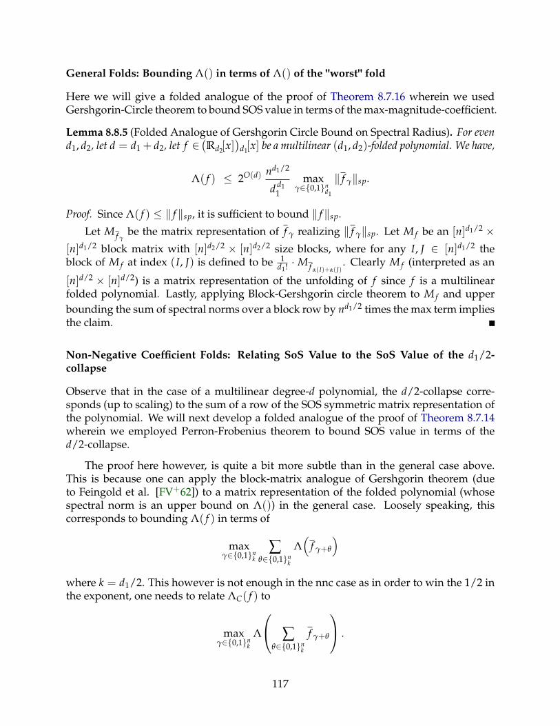
General Folds: Bounding Λ() in terms of Λ() of the "worst" fold
Here we will give a folded analogue of the proof of Theorem 8.7.16 wherein we usedGershgorin-Circle theorem to bound SOS value in terms of the max-magnitude-coefficient.
Lemma 8.8.5 (Folded Analogue of Gershgorin Circle Bound on Spectral Radius). For evend1, d2, let d = d1 + d2, let f ∈
(Rd2[x]
)d1[x] be a multilinear (d1, d2)-folded polynomial. We have,
Λ( f ) ≤ 2O(d) nd1/2
d d11
maxγ∈0,1n
d1
‖ f γ‖sp.
Proof. Since Λ( f ) ≤ ‖ f ‖sp, it is sufficient to bound ‖ f ‖sp.
Let M f γbe the matrix representation of f γ realizing ‖ f γ‖sp. Let M f be an [n]d1/2 ×
[n]d1/2 block matrix with [n]d2/2 × [n]d2/2 size blocks, where for any I, J ∈ [n]d1/2 theblock of M f at index (I, J) is defined to be 1
d1! ·M f α(I)+α(J). Clearly M f (interpreted as an
[n]d/2 × [n]d/2) is a matrix representation of the unfolding of f since f is a multilinearfolded polynomial. Lastly, applying Block-Gershgorin circle theorem to M f and upperbounding the sum of spectral norms over a block row by nd1/2 times the max term impliesthe claim.
Non-Negative Coefficient Folds: Relating SoS Value to the SoS Value of the d1/2-collapse
Observe that in the case of a multilinear degree-d polynomial, the d/2-collapse corre-sponds (up to scaling) to the sum of a row of the SOS symmetric matrix representation ofthe polynomial. We will next develop a folded analogue of the proof of Theorem 8.7.14wherein we employed Perron-Frobenius theorem to bound SOS value in terms of thed/2-collapse.
The proof here however, is quite a bit more subtle than in the general case above.This is because one can apply the block-matrix analogue of Gershgorin theorem (dueto Feingold et al. [FV+62]) to a matrix representation of the folded polynomial (whosespectral norm is an upper bound on Λ()) in the general case. Loosely speaking, thiscorresponds to bounding Λ( f ) in terms of
maxγ∈0,1n
k∑
θ∈0,1nk
Λ(
f γ+θ
)where k = d1/2. This however is not enough in the nnc case as in order to win the 1/2 inthe exponent, one needs to relate ΛC( f ) to
maxγ∈0,1n
k
Λ
∑θ∈0,1n
k
f γ+θ
.
117
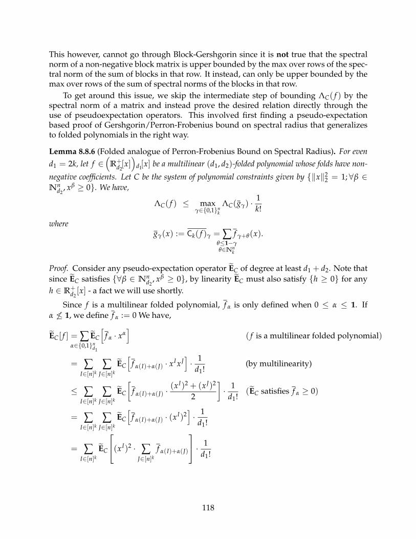
This however, cannot go through Block-Gershgorin since it is not true that the spectralnorm of a non-negative block matrix is upper bounded by the max over rows of the spec-tral norm of the sum of blocks in that row. It instead, can only be upper bounded by themax over rows of the sum of spectral norms of the blocks in that row.
To get around this issue, we skip the intermediate step of bounding ΛC( f ) by thespectral norm of a matrix and instead prove the desired relation directly through theuse of pseudoexpectation operators. This involved first finding a pseudo-expectationbased proof of Gershgorin/Perron-Frobenius bound on spectral radius that generalizesto folded polynomials in the right way.
Lemma 8.8.6 (Folded analogue of Perron-Frobenius Bound on Spectral Radius). For evend1 = 2k, let f ∈
(R+
d2[x])
d1[x] be a multilinear (d1, d2)-folded polynomial whose folds have non-
negative coefficients. Let C be the system of polynomial constraints given by ‖x‖22 = 1; ∀β ∈
Nnd2
, xβ ≥ 0. We have,
ΛC( f ) ≤ maxγ∈0,1n
k
ΛC(gγ) ·1k!
wheregγ(x) := Ck( f )γ = ∑
θ≤1−γθ∈Nn
k
f γ+θ(x).
Proof. Consider any pseudo-expectation operator EC of degree at least d1 + d2. Note thatsince EC satisfies ∀β ∈ Nn
d2, xβ ≥ 0, by linearity EC must also satisfy h ≥ 0 for any
h ∈ R+d2[x] - a fact we will use shortly.
Since f is a multilinear folded polynomial, f α is only defined when 0 ≤ α ≤ 1. Ifα 6≤ 1, we define f α := 0 We have,
EC[ f ] = ∑α∈0,1n
d1
EC
[f α · xα
]( f is a multilinear folded polynomial)
= ∑I∈[n]k
∑J∈[n]k
EC
[f α(I)+α(J) · xI x J
]· 1
d1!(by multilinearity)
≤ ∑I∈[n]k
∑J∈[n]k
EC
[f α(I)+α(J) ·
(xI)2 + (x J)2
2
]· 1
d1!(EC satisfies f α ≥ 0)
= ∑I∈[n]k
∑J∈[n]k
EC
[f α(I)+α(J) · (xI)2
]· 1
d1!
= ∑I∈[n]k
EC
(xI)2 · ∑J∈[n]k
f α(I)+α(J)
· 1d1!
118
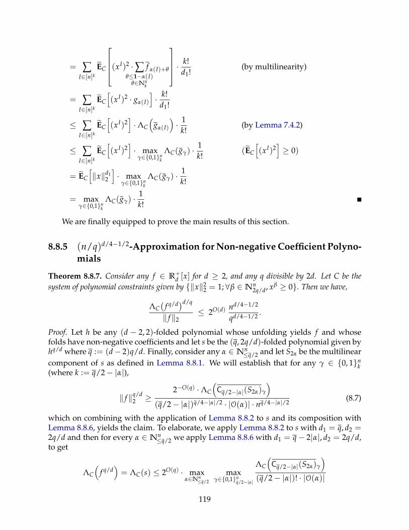
= ∑I∈[n]k
EC
(xI)2 ·∑θ≤1−α(I)
θ∈Nnk
f α(I)+θ
· k!d1!
(by multilinearity)
= ∑I∈[n]k
EC
[(xI)2 · gα(I)
]· k!
d1!
≤ ∑I∈[n]k
EC
[(xI)2
]·ΛC
(gα(I)
)· 1
k!(by Lemma 7.4.2)
≤ ∑I∈[n]k
EC
[(xI)2
]· max
γ∈0,1nk
ΛC(gγ) ·1k!
(EC
[(xI)2
]≥ 0)
= EC
[‖x‖d1
2
]· max
γ∈0,1nk
ΛC(gγ) ·1k!
= maxγ∈0,1n
k
ΛC(gγ) ·1k!
We are finally equipped to prove the main results of this section.
8.8.5 (n/q)d/4−1/2-Approximation for Non-negative Coefficient Polyno-mials
Theorem 8.8.7. Consider any f ∈ R+d [x] for d ≥ 2, and any q divisible by 2d. Let C be the
system of polynomial constraints given by ‖x‖22 = 1; ∀β ∈Nn
2q/d, xβ ≥ 0. Then we have,
ΛC(
f q/d)d/q
‖ f ‖2≤ 2O(d) nd/4−1/2
qd/4−1/2 .
Proof. Let h be any (d − 2, 2)-folded polynomial whose unfolding yields f and whosefolds have non-negative coefficients and let s be the (q, 2q/d)-folded polynomial given byhq/d where q := (d− 2)q/d. Finally, consider any α ∈Nn
≤q/2 and let S2α be the multilinearcomponent of s as defined in Lemma 8.8.1. We will establish that for any γ ∈ 0, 1n
k(where k := q/2− |α|),
‖ f ‖q/d2 ≥
2−O(q) ·ΛC
(Cq/2−|α|(S2α)γ
)(q/2− |α|)q/4−|α|/2 · |O(α)| · nq/4−|α|/2
(8.7)
which on combining with the application of Lemma 8.8.2 to s and its composition withLemma 8.8.6, yields the claim. To elaborate, we apply Lemma 8.8.2 to s with d1 = q, d2 =2q/d and then for every α ∈ Nn
≤q/2 we apply Lemma 8.8.6 with d1 = q− 2|α|, d2 = 2q/d,to get
ΛC
(f q/d
)= ΛC(s) ≤ 2O(q) · max
α∈Nn≤q/2
maxγ∈0,1n
q/2−|α|
ΛC
(Cq/2−|α|(S2α)γ
)(q/2− |α|)! · |O(α)|
119
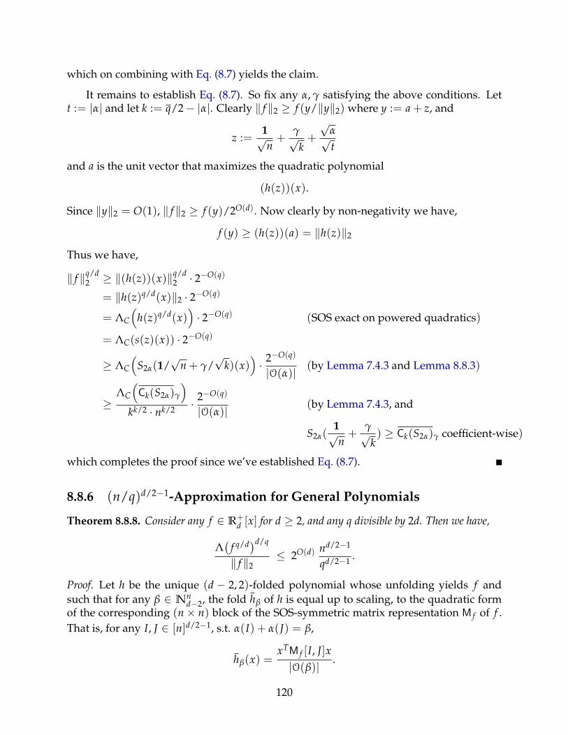
which on combining with Eq. (8.7) yields the claim.
It remains to establish Eq. (8.7). So fix any α, γ satisfying the above conditions. Lett := |α| and let k := q/2− |α|. Clearly ‖ f ‖2 ≥ f (y/‖y‖2) where y := a + z, and
z :=1√n+
γ√k+
√α√t
and a is the unit vector that maximizes the quadratic polynomial
(h(z))(x).
Since ‖y‖2 = O(1), ‖ f ‖2 ≥ f (y)/2O(d). Now clearly by non-negativity we have,
f (y) ≥ (h(z))(a) = ‖h(z)‖2
Thus we have,
‖ f ‖q/d2 ≥ ‖(h(z))(x)‖q/d
2 · 2−O(q)
= ‖h(z)q/d(x)‖2 · 2−O(q)
= ΛC
(h(z)q/d(x)
)· 2−O(q) (SOS exact on powered quadratics)
= ΛC(s(z)(x)) · 2−O(q)
≥ ΛC
(S2α(1/
√n + γ/
√k)(x)
)· 2−O(q)
|O(α)| (by Lemma 7.4.3 and Lemma 8.8.3)
≥ΛC
(Ck(S2α)γ
)kk/2 · nk/2 · 2−O(q)
|O(α)| (by Lemma 7.4.3, and
S2α(1√n+
γ√k) ≥ Ck(S2α)γ coefficient-wise)
which completes the proof since we’ve established Eq. (8.7).
8.8.6 (n/q)d/2−1-Approximation for General Polynomials
Theorem 8.8.8. Consider any f ∈ R+d [x] for d ≥ 2, and any q divisible by 2d. Then we have,
Λ(
f q/d)d/q
‖ f ‖2≤ 2O(d) nd/2−1
qd/2−1 .
Proof. Let h be the unique (d − 2, 2)-folded polynomial whose unfolding yields f andsuch that for any β ∈ Nn
d−2, the fold hβ of h is equal up to scaling, to the quadratic formof the corresponding (n× n) block of the SOS-symmetric matrix representation M f of f .That is, for any I, J ∈ [n]d/2−1, s.t. α(I) + α(J) = β,
hβ(x) =xTM f [I, J]x|O(β)| .
120
Let s be the (q, 2q/d)-folded polynomial given by hq/d where q := (d− 2)q/d. Considerany α ∈ Nn
≤q/2 and γ ∈ 0, 1nq−2|α|, and let S2α be the multilinear component of s as
defined in Lemma 8.8.1. Below we will show,
‖ f ‖q/d2 ≥
2−O(q) · ‖(S2α)γ‖sp
(q− 2|α|)q/2−|α| · |O(α)|(8.8)
which would complete the proof after applying Lemma 8.8.2 to s and composing theresult with Lemma 8.8.5. To elaborate, we apply Lemma 8.8.2 to s with d1 = q, d2 = 2q/dand then for every α ∈Nn
≤q/2 we apply Lemma 8.8.5 with d1 = q− 2|α|, d2 = 2q/d, to get
Λ(
f q/d)= Λ(s) ≤ 2O(q) · max
α∈Nn≤q/2
maxγ∈0,1n
q−2|α|
‖(S2α)γ‖sp
(q− 2|α|)q−2|α| · |O(α)|
which on combining with Eq. (8.8) yields the claim.
Fix any α, γ satisfying the above conditions. Let k := q− 2α. Let t := |α|, and let
z := Ξ · 1√k· γ 1
2α + 1 b +
√α ζ√
t
Ξ is an independent and uniformly randomly chosen (k + 1)-th root of unity, and forany i ∈ [n], ζi is an independent and uniformly randomly chosen (2αi + 1)-th root ofunity, and for any i ∈ [n], bi is an independent Bernoulli(p) random variable (p is aparameter that will be set later). By Lemma 8.7.7 and definition of h, we see that for anyy, ‖ f ‖c
2 ≥ ‖(h(y))(x)‖c2. Thus we have,
‖ f ‖q/d2 = ‖ f q/d‖2
≥ ‖ f q/d‖c2 · 2−O(q) (by Lemma 8.7.8)
≥ maxp∈[0,1]
E[‖h(z)q/d(x)‖2
]· 2−O(q) (by Lemma 8.7.7)
= maxp∈[0,1]
E[‖h(z)q/d(x)‖sp
]· 2−O(q) (SOS exact on powered quadratics)
= maxp∈[0,1]
E
‖h(z)q/d(x) · Ξ ·∏i∈[n]
ζi‖sp
· 2−O(q)
≥ maxp∈[0,1]
∥∥∥∥E
h(z)q/d(x) · Ξ ·∏i∈[n]
ζi
∥∥∥∥sp· 2−O(q)
= maxp∈[0,1]
∥∥∥∥E
(s(z))(x) · Ξ ·∏i∈[n]
ζi
∥∥∥∥sp· 2−O(q)
= maxp∈[0,1]
∥∥∥∥ pk · (S2α(γ/√
k))(x)|O(α)| + r(p)
∥∥∥∥sp· 2−O(q) (by Lemma 8.8.4, deg(r) < k)
121
= maxp∈[0,1]
∥∥∥∥ pk · (S2α)γ(x)kk/2 · |O(α)|
+ r(p)∥∥∥∥
sp· 2−O(q)
≥‖(S2α)γ‖sp
kk/2 · |O(α)|· 2−O(q+k) (Chebyshev Inequality - Lemma 8.7.5)
where the last inequality follows by the following argument: one would like to show thatthere always exists p ∈ [0, 1] such that ‖pk · hk(x) + . . . p0 · h0(x))‖sp ≥ ‖hk(x)‖sp · 2−O(k).So let p be such that |pk · uT Mkv + . . . p0 · uT M0v| ≥ |uT Mkv| · 2−O(k) (such a p exists byChebyshev inequality) where Mk is the matrix representation of hk(x) realizing ‖hk‖spand u, v are the maximum singular vectors of Mk. Mk−1, . . . , M0 are arbitrary matrix rep-resentations of hk−1, . . . h0 respectively. But pk ·Mk + . . . p0 ·M0 is a matrix representationof pk · hk + . . . p0 · h0. Thus ‖pk · hk + . . . p0 · h0‖sp ≥ |uT Mkv|/2−O(k) = ‖hk‖sp · 2−O(q).
This completes the proof as we’ve established Eq. (8.8).
8.8.7 Algorithms
It is straightforward to extract algorithms from the proofs of Theorem 8.8.7 and Theo-rem 8.8.8.
Non-negative coefficient polynomials
Let f be a degree-d polynomial with non-negative coefficients and let h be a (d − 2, 2)-folded polynomial whose unfolding yields f . Consider any q divisible by 2d and let q :=(d− 2)q/d. Pick and return the best vector from the set
1√n+
√α√|α|
+γ√|γ|
+ arg max∥∥∥∥h
(1√n+
√α√|α|
+γ√|γ|
)(x)∥∥∥∥
2
∣∣∣ α ∈Nn≤q/2, γ ∈Nn
q/2−|α|
General Polynomials
Let f be a degree-d polynomial and let h be the unique (d− 2, 2)-folded polynomial whoseunfolding yields f and such that for any β ∈Nn
d−2, the fold hβ of h is equal up to scaling,to the quadratic form of the corresponding (n × n) block of the SOS-symmetric matrixrepresentation M f of f . That is, for any I, J ∈ [n]d/2−1, s.t. α(I) + α(J) = β,
hβ(x) =xTM f [I, J]x|O(β)| .
Consider any q divisible by 2d and let q := (d− 2)q/d. Let the set S be defined by,
S :=
Ξ · 1√
|γ|· γ 1
2α + 1 b +
√α ζ√|α|
∣∣∣∣∣ Ξ ∈ Ωk+1, ζi ∈ Ω2αi+1, b ∈ 0, 1n,
α ∈Nn≤q/2, γ ∈ 0, 1n
q−2|α|
122
where Ωp denotes the set of p-th roots of unity. Pick and return the best vector from theset
c1 · y + c2 · arg max ‖(h(y))(x)‖2
∣∣∣ y ∈ S, c1 ∈ [−(d− 2), (d− 2)], c2 ∈ [−2, 2]
Note that one need only search through all roots of unity vectors ζ supported on Supp γand all 0, 1-vectors b supported on Supp α. Lemma 8.7.7 can trivially be made construc-tive in time 2O(q). Lastly, to go from complexes to reals, Lemma 8.7.8 can trivially be madeconstructive using 2O(d) time. Thus the algorithm runs in time nO(q).
8.9 Constant Level Lower Bounds for Polynomials with Non-negative Coefficients
Let G = (V, E) be a random graph drawn from the distribution Gn,p for p ≥ n−1/3. LetC ⊆ (V
4) be the set of 4-cliques in G. The polynomial f is defined as
f (x1, . . . , xn) := ∑i1,i2,i3,i4∈C
xi1 xi2 xi3 xi4 .
Clearly, f is multilinear and every coefficient of f is nonnegative. In this section, we provethe following two lemmas that establish a polynomial gap between ‖ f ‖2 and Λ( f ).
Lemma 8.9.1 (Soundness). With probability at least 1− 1n over the choice of the graph G, we
have ‖ f ‖2 ≤ n2p6 · (log n)O(1).
Lemma 8.9.2 (Completeness). With probability at least 1− 1n over the choice of the graph G, we
have
Λ( f ) ≥ Ω(n1/2 · p
log2 n
)when p ∈ [n−1/3, n−1/4].
Note that the gap between the two quantities if Ω(n1/6) when p = n−1/3, which isthe choice we make.
8.9.1 Upper Bound on ‖ f ‖2
Reduction to counting shattered cliques
We say that an ordered 4-clique (i1, . . . , i4) is shattered by 4 disjoint sets Z1, . . . , Z4 if foreach k ∈ [4], ik ∈ Zk. Let Yj1 , . . . , Yj4 be the sets containing the coordinates i1, . . . , i4. LetCG denote the set of (ordered) 4-cliques in G, and let CG(Z1, Z2, Z3, Z4) denote the set ofcliques shattered by Z1, . . . , Z4.
We reduce the problem of bounding ‖ f ‖2, to counting shattered 4-cliques.
123
Claim 8.9.3. There exist disjoint sets Z1, . . . , Z4 ⊆ [n] such that
|CG(Z1, Z2, Z3, Z4)| ≥(
4
∏k=1|Zk|
)1/2
·O(‖ f ‖2
(log n)4
).
Proof. Let x∗ ∈ Sn−1 be the vector that maximizes f . Without loss of generality, assumethat every coordinate of x∗ is nonnegative. Let y∗ be another unit vector defined as
y∗ :=
(x∗ + 1/
√n)
‖x∗ + 1/√
n‖2.
Since both x∗ and 1√n are unit vectors, the denominator is at most 2. This implies that
f (y∗) ≥ f (x∗)24 , and each coordinate of y∗ is at least 1
2√
n . For 1 ≤ j ≤ log2 n, let Yj be the set
Yj :=
i ∈ [n] | 2−j < y∗i ≤ 2−(j−1)
.
The sets Y1, . . . , Ylog2 n partition [n]. Since 1 = ∑i∈[n] y2i > |Yj| · 2−2j, we have for each
j, |Yj| ≤ 22j. Let Z1, Z2, Z3, and Z4 be pairwise disjoint random subsets of [n] chosen asfollows:
- Randomly partition each Yj to Yj,1, . . . , Yj,4 where each element of Yj is put into ex-actly one of Yj,1, . . . , Yj,4 uniformly and independently.
- Sample r1, . . . , r4 independently and randomly from 1, . . . , log2 n.
- For k = 1, . . . , 4, take Zk := Yrk,k
We use P to denote random partitions(
Yj,1, . . . , Yj,4)
j∈[log n] and r to denote the randomchoices r1, . . . , r4. Note that the events ik ∈ Zk are independent for different k, and thatZ1, . . . , Z4 are independent given P . Thus, we have
EP ,r
[1 [(i1, i2, i3, i4) is shattered]√
|Z1| |Z2| |Z3| |Z4|
]= E
P
[4
∏k=1
Erk
[1 [ik ∈ Zk]√|Zk|
]]
= EP
4
∏k=1
Erk
1 [rk = jk] · 1[ik ∈ Yjk,k
]√∣∣Yjk,k∣∣
≥ E
P
4
∏k=1
Erk
1 [rk = jk] · 1[ik ∈ Yjk,k
]√∣∣Yjk
∣∣
= EP
4
∏k=1
1log n
·1[ik ∈ Yjk,k
]√∣∣Yjk
∣∣
124
= EP
4
∏k=1
1log n
·1[ik ∈ Yjk,k
]√∣∣Yjk
∣∣
=1
(4 log n)4 ·1√∣∣Yj1
∣∣ ∣∣Yj2
∣∣ ∣∣Yj3
∣∣ ∣∣Yj4
∣∣≥ 1
(4 log n)4 · 2j1+j2+j3+j4
≥ 1
(8 log n)4 · y∗i1y∗i2y∗i3y∗i4 .
Then, by linearity of expectation,
EP ,r
[|CG(Z1, Z2, Z3, Z4)|√|Z1| |Z2| |Z3| |Z4|
]≥ 1
(8 log n)4 · ∑(i1,...,i4)∈CG
y∗i1y∗i2y∗i3y∗i4
=4!
(8 log n)4 · f (y∗)
≥ 4!(16 log n)4 · f (x∗) =
4!(16 log n)4 · ‖ f ‖2 ,
which proves the claim.
We will show that with high probability, G satisfies the property that every four dis-joint sets Z1, . . . , Z4 ⊆ V shatter at most O
(√|Z1||Z2||Z3||Z4| · n2p6 · (log n)O(1)
)cliques,
proving Lemma 8.9.1.
Counting edges and triangles
For a vertex i ∈ [n], we use N(i) to denote the set of vertices in the graph G. For easeof notation, we use a . b to denote a ≤ b · (log n)O(1). We first collect some simpleconsequences of Chernoff bounds.
Claim 8.9.4. Let G ∼ Gn,p with p ≥ n−1/3. Then, with probability 1− 1n , we have
- For all distinct i1, i2 ∈ [n], |N(i1) ∩ N(i2)| . np2.
- For all distinct i1, i2, i3 ∈ [n], |N(i1) ∩ N(i2) ∩ N(i3)| . np3.
- For all sets S1, S2 ⊆ [n], |E(S1, S2)| . max |S1| |S2| p, |S1|+ |S2|.
We also need the following bound on the number of triangles shattered by three dis-joint sets S1, S2 and S3, denoted by ∆G(S1, S2, S3). As for 4-cliques, a triangle is said to beshattered if it has exactly one vertex in each the sets.
125
Claim 8.9.5. Let G ∼ Gn,p with p ≥ n−1/3. Then, with probability 1− 1n , for all disjoint sets
S1, S2, S3 ⊆ [n]
|∆G(S1, S2, S3)| . |S3|+ |E(S1, S2)| ·(
np3 · |S3|)1/2
.
Proof. With probability at least 1− 1n , G satisfies the conclusion of Claim 8.9.4. Fix such
a G, and consider arbitrary subsets S1, S2, S3 ⊆ V. Consider the bipartite graph H wherethe left side vertices correspond to edges in E(S1, S2), the right side vertices correspondto vertices in S3, and there is an edge from (i1, i2) ∈ E(S1, S2) to i3 ∈ S3 when both(i1, i3), (i2, i3) ∈ E. Clearly, |∆G(S1, S2, S3)| is equal to the number of edges in H.
Consider two different edges (i1, i2), (i′1, i′2) ∈ E(S1, S2). These two edges are incidenton at least 3 distinct vertices, say i1, i2, i′1. Hence, the number of vertices i3 ∈ [n] thatare adjacent to all i1, i2, i′1, i′2 in G is at most |N(i1) ∩ N(i2) ∩ N(i′1)| . np3. This givesthat the number of pairs triangles sharing a common vertex in S3 is at most |E(S1, S2)|2 ·np3(log n)O(1).
Let dH(i3) denote the degree of a vertex i3 in H, and let ∆ denote the number ofshattered triangles. Counting the above pairs of triangles using the degrees gives
∑i3∈S3
(dH(i3)
2
). |E(S1, S2)|2 · np3 .
An application of Cauchy-Schwarz gives
∆2 − ∆ · |S3| . |S3| · |E(S1, S2)|2 · np3 ,
which proves the claim.
Bounding 4-clique Density
Let G ∼ Gn,p be a graph satisfying the conclusions of Claims Claim 8.9.4 and Claim 8.9.5.Let S1, . . . , S4 ⊆ [n] be disjoint sets with sizes n1 ≤ n2 ≤ n3 ≤ n4. We consider two cases:
- Case 1: |E(S1, S2)| . n1n2pNote that each edge (i1, i2) can only participate in at most |N(i1) ∩ N(i2)| triangles,and each triangle (i1, i2, i3) can only be extended to at most |N(i1) ∩ N(i2) ∩ N(i3)|4-cliques. Thus, Claim Claim 8.9.4 gives
|CG(S1, S2, S3, S4)| . n1n2p · np2 · np3 . (n1n2n3n4)1/2 · n2p6 .
- Case 2: |E(S1, S2)| . n1 + n2
Claim Claim 8.9.5 gives
|∆G(S1, S2, S3)| . n3 + (n1 + n2) ·(
n3 · np3)1/2
,
126
which together with Claim Claim 8.9.4 implies
|CG(S1, S2, S3, S4)| . n3 · np3 + (n1 + n2) · n1/23 ·
(np3)3/2
.
Considering the first term, we note that
n3 · np3 ≤ (n3n4)1/2 · n2p6 ≤ (n1n2n3n4)
1/2 · n2p6 ,
since n3 ≤ n4 and np3 ≥ 1. Similarly, for the second term, we have
(n1 + n2) · n1/23 ·
(np3)3/2
≤ 2(n2n3n4)1/2 ·
(np3)3/2
≤ 2 · (n1n2n3n4)1/2 · n2p6 .
Combined with Claim Claim 8.9.3, this completes the proof of Lemma 8.9.1.
8.9.2 Lower Bound on Λ( f )
Recall that given a random graph G = ([n], E) drawn from the distribution Gn,p, thepolynomial f is defined as
f (x1, . . . , xn) := ∑i1,i2,i3,i4∈C
xi1 xi2 xi3 xi4 ,
where C ⊆ ([n]4 ) is the set of 4-cliques in G. Let A ∈ R[n]2×[n]2 be the natural matrixrepresentation of 24 f (corresponding to ordered copies of cliques) with
A[(i1, i2), (i3, i4)] =
1 if i1, . . . , i4 ∈ C0 otherwise
Let E′ ⊆ [n]2 be the set of ordered edges i.e., (i1, i2) ∈ E′ if and only if i1, i2 ∈ E. Notethat |E′| = 2m where m is the number of edges in G. All nonzero entries of A are containedin the principal submatrix AE′ , formed by the rows and columns indexed by E′.
A simple lower bound on ‖ f ‖sp
We first give a simple proof that ‖ f ‖sp ≥√
n2p5 with high probability.
Lemma 8.9.6. ‖ f ‖sp ≥ Ω(√
n2p5) = Ω(n1/6) with high probability.
Proof. Consider any matrix representation M of 24 f and its principal submatrix ME′ . Itis easy to observe that the Frobenius norm of ME′ satisfies ‖ME′‖2
F ≥ 24 |C|, minimizedwhen M = A. Since ‖ME′‖2
F ≤ |E′| · ‖AE′‖22, we have that with high probability,
‖A‖2 ≥ ‖AE′‖2 ≥
√24 |C|2|E| = Ω
(√n4p6√n2p
)= Ω
(√n2p5
).
127
Lower bound for the stronger relaxation computing Λ( f )
We now prove Lemma 8.9.2, which says that Λ( f ) ≥ n1/6
log2 nwith high probability. In order
to show a lower bound, we look at the dual SDP for computing Λ( f ), which is a maxi-mization problem over positive semidefinite, SoS-symmetric matrices M with Tr(M) = 1.We exhibit such a matrix M ∈ R[n]2×[n]2 for which the value of the objective 〈A,M〉 is large.
For large 〈A,M〉, one natural attempt is to take M to be A and modify it to satisfy otherconditions. Note that A is already SoS-symmetric. However, Tr(A) = 0, which impliesthat the minimum eigenvalue is negative.
Let λmin be the minimum eigenvalue of A, which is also the minimum eigenvalue ofAE′ . Let IE′ ∈ R[n]2×[n]2 be such that I[(i1, i2), (i1, i2)] = 1 if (i1, i2) ∈ E′ and all otherentries are 0. Note that IE′ is a diagonal matrix with Tr(IE′) = 2m. Adding −λmin · IE′ toA makes it positive semidefinite, so setting
M =A− λmin IE′
Tr(A− λmin IE′)=
A− λmin IE′
−2mλmin=
A+ |λmin| · IE′
2m · |λmin|(8.9)
makes sure that M is positive semidefinite, Tr(M) = 1, and 〈A,M〉 = 12|C|m·|λmin| (each 4-
clique in C contributes 24). Since |C| = Θ(n4p6) and m = Θ(n2p) with high probability, if|λmin| = O(np5/2), 〈A,M〉 = Θ
(n2p5/2), which is Ω(n1/6) when p = Ω(n−1/3).
The M defined in Eq. (8.9) does not directly work since it is not SoS-symmetric. How-ever, the following claim proves that this issue can be fixed by losing a factor 2 in 〈A,M〉.
Claim 8.9.7. There exists M such that it is SoS-symmetric, positive semidefinite with Tr(M) = 1,and 〈A,M〉 ≥ 6|C|
m·|λmin| .
Proof. Let QE′ ∈ R[n]2×[n]2 be the matrix such that
- For (i1, i2) ∈ E′, QE′ [(i1, i1), (i2, i2)] = QE′ [(i2, i2), (i1, i1)] = 1.
- For i ∈ [n], QE′ [(i, i), (i, i)] = degG(i), where degG(i) denotes the degree of i in G.
- All other entries are 0.
We claim that IE′ + QE′ is SoS-symmetric: (IE′ + QE′)[(i1, i2), (i3, i4)] has a nonzero entryif and only if i1 = i2 = i3 = i4 or two different numbers j1, j2 appear exactly twice and(j1, j2) ∈ E′ (in this case (IE′ + QE′)[(i1, i2), (i3, i4)] = 1). Since A is SoS-symmetric, soA+ |λmin| · (IE′ + QE′) is also SoS-symmetric.
It is easy to see that QE′ is diagonally dominant, and hence positive semidefinite.Since we already argued that A+ |λmin| · IE′ is positive semidefinite, A+ |λmin| · (IE′ +QE′) is also positive semidefinite. Also, Tr(QE′) = ∑i∈[n] degG(i) = 2m. Thus, we take
M =A+ |λmin| · (IE′ + QE′)
Tr(A+ |λmin| · (IE′ + QE′))=
A+ |λmin| · IE′
4m · |λmin|.
128
By the above arguments, we have that M that is PSD, SoS-symmetric with Tr(M) = 1, and
〈A,M〉 = 6|C|m · |λmin|
as desired.
It only remains to bound λmin, which is the minimum eigenvalue of A and AE′ . Forp in the range [n−1/3, n−1/4], we will show a bound of O(n3/2p4) below, which whencombined with the above claim, completes the proof of Lemma 8.9.2.
Bounding the smallest eigenvalue via the trace method
Our estimate |λmin| = O(np5/2) is based on the following observation: AE′ is a 2m× 2mrandom matrix where each row and column is expected to have Θ(n2p5) ones (the ex-pected number of 4-cliques an edge participates in). An adjacency matrix of a randomgraph with average degree d has a minimum eigenvalue −Θ(
√d), hence the estimate
|λmin| = O(np5/2). Even though AE′ is not sampled from a typical random graph model(and even E′ is a random variable), we will be able to prove the following weaker esti-mate, which suffices for our purposes.
Lemma 8.9.8. With high probability over the choice of the graph G, we have
|λmin| =
O(n3/2 · p4) for p ∈
[n−1/3, n−1/4]
O(n5/3 · p14/3) for p ∈
[n−1/4, 1/2
]Proof. Instead of AE′ , we directly study A to bound λmin. For simplicity, we considerthe following matrix A, where each row and column is indexed by an unordered pairi, j ∈ ([n]2 ), and A[i1, i2, i3, i4] = 1 if and only if i1, i2, i3, i4 form a 4-clique. A hasonly zero entries in the rows or columns indexed by (i, i) for all i ∈ [n], and for two pairsi1 6= i2 and i3 6= i4, we have
A[i1, i2, i3, i4] :=14· A[(i1, i2), (i3, i4)] + A[(i1, i2), (i4, i3)]
+14· A[(i2, i1), (i3, i4)] + A[(i2, i1), (i4, i3)] .
Therefore, |λmin (A)| ≤ 4 ·∣∣∣λmin
(A)∣∣∣ and it suffices to bound the minimum eigenvalue
of A. We consider the matrix NE := A− p4 · JE, where JE ∈ R([n]2 )×([n]2 ) is such that
JE[i1, i2, i3, i4] =
1 if i1, i2, i3, i4 ∈ E0 otherwise
.
129
Since JE is a rank-1 matrix with a positive eigenvalue, the minimum eigenvalues of A andNE are the same. In summary, NE is the following matrix.
NE[i1, i2, i3, i4] =
1− p4 if i1, i2, i3, i4 ∈ C−p4 if i1, i2, i3, i4 /∈ C but i1, i2, i3, i4 ∈ E0 otherwise
We use the trace method to bound ‖NE‖2, based on the observation that for every even
r ∈ N, ‖NE‖2 ≤(Tr((NE)
r))1/r
. Fix an even r ∈ N. The expected value of the trace canbe represented as
E[Tr((NE)
r)]
= E
∑I1,...,Ir∈([n]2 )
r
∏k=1
NE[Ik, Ik+1]
= ∑I1,...,Ir∈([n]2 )
E
[r
∏k=1
NE[Ik, Ik+1]
]
where each I j =
ij1, ij
2
∈ ([n]2 ) is an edge of the complete graph on n vertices (call it a
potential edge) and Ir+1 := I1.Fix r potential edges I1, . . . , Ir, let t := ∏r
k=1 NE[Ik, Ik+1], and consider E[t]. Let E0 :=I1, . . . , Ir be the set of distinct edges represented by I1, . . . , Ir. Note that the expectedvalue is 0 if one of I j does not become an edge. Therefore, E[t] = p|E0| ·E[t | E0 ⊆ E].
Let D ⊆ [r] be the set of j ∈ [r] such that all four vertices in I j and I j+1 are distinct i.e.,
D :=
j ∈ [r] |∣∣∣ij
1, ij2, ij+1
1 , ij+12
∣∣∣ = 4
.
For j ∈ [r] \ D, ij1, ij
2, ij+11 , ij+1
2 cannot form a 4-clique, so given that I j, I j+1 ∈ E, we have
NE[I j, I j+1] = −p4. For j ∈ D, let Ej :=
ij1, ij+1
1
,
ij1, ij+1
2
,
ij2, ij+1
1
,
ij2, ij+1
2
\ E0
be the set of edges in the 4-clique created by
ij1, ij
2, ij+11 , ij+1
2
except ones in E0. Then
E [t] = p|E0| ·E [t|E0 ⊆ E] = p|E0| · (−p4)r−|D| ·E[
∏k∈D
NE[Ik, Ik+1] | E0 ⊆ E
].
Suppose there exists j ∈ D such that∣∣Ej∣∣ = 4 and Ej ∩ (∪j′∈D\jEj′) = ∅. Then, given
that E0 ⊆ E, NE[I j, I j+1] is independent of allNE[Ik, Ik+1]
k∈D\j
, and
E[NE[I j, I j+1]|E0 ⊆ E
]= p4(1− p4) + (1− p4)(−p4) = 0 .
Therefore, E[t] = 0 unless for all j ∈ D, either |Ej| ≤ 3 or there exists j′ ∈ D \ j withEj ∩ Ej′ 6= ∅.
Let ED :=⋃
j∈D Ej. Note that E0 and ED completely determines t. E[t] can be writtenas
p|E0| · (−p4)r−|D| ·E[
∏k∈D
NE[Ik, Ik+1] | E0 ⊆ E
]
130
= p|E0| · (−p4)r−|D| · ∑F⊆ED
(p|F|(1− p)|ED|−|F| ·E
[∏k∈D
NE[Ik, Ik+1] | E0 ⊆ E, ED ∩ E = F
])= p|E0| · (−p4)r−|D| · ∑
F⊆ED
(p|F|(1− p)|ED|−|F| · (1− p4)|D|−a(F)(−p4)a(F)
),
where a(F) denotes the number of j ∈ D with Ej 6⊆ F. Since ED ⊆ F ∪(⋃
j:Ej 6⊆F Ej))
and4a(F) + |F| ≥ |ED|, we have
E [t] = p|E0| · (−p4)r−|D| · ∑F⊆ED
(p|F|(1− p)|ED|−|F| · (1− p4)|D|−a(F)(−p4)a(F)
)≤ p|E0| · (p4)r−|D| · 2|ED| · p|ED|
≤ 24r · p4(r−D)+|E0|+|ED| .
We now count the number of terms which contribute to the sum. Fix a graph H with rlabelled edges I1, . . . , Ir (possibly repeated) and q := q(H) vertices, without any isolatedvertex (so q ≤ 2r). There are at most (q
2)r ≤ (2r)2r such graphs. Then I1, . . . , Ir, as edges
in ([n]2 ), are determined by a map VH → [n]. There are at most nq such mappings.Let E0 := E0(H), D := D(H), Ej := Ej(H), E′ := E′(H) be defined as before. Note
that E0 is set the edges of H. As observed before, the contribution from H is 0 if thereexists j ∈ D such that |Ej| = 4 and Ej is disjoint from Ej′j′∈D\j. Let H be the set of Hthat has nonzero contribution. Then,
E[Tr((
NE
)r)]= ∑
I1,...,Ir∈([n]2 )
E
[r
∏k=1
NE[Ik, Ik+1]
]
≤ ∑H∈H
nq(H) · 24r · p4(r−D(H))+|E0(H)|+|ED(H)|
≤ (2r)2r ·maxH∈H
(nq(H)24r · p4(r−D(H))+|E0(H)|+|ED(H)|
)≤ (8r)2r ·max
H∈H
(nq(H)p4(r−D(H))+|E0(H)|+|ED(H)|
)We will prove the following bound on the maximum contribution of any H ∈ H.
Claim 8.9.9. LetH be defined as above. Then, for all H ∈ H, we have
nq(H)p4(r−D(H))+|E0(H)|+|ED(H)| ≤ n2 · Brp ,
where
Bp =
n3/2 · p4 for p ∈
[n−1/3, n−1/4]
n5/3 · p14/3 for p ∈[n−1/4, 1/2
] .
Using the above claim, we can bound E[Tr((
NE
)r)] as
E[Tr((
NE
)r)]≤ (8r)2r ·max
H∈H
(nq(H)p4(r−D(H))+|E0(H)|+|ED(H)|)
131
≤ (8r)2r · n2 · Brp ,
where Bp is given by Claim Claim 8.9.9 for different ranges of p. By Markov’s inequality,
we get that with probability 1− 1n , we have Tr
((NE
)r)≤ (8r)2r · n3 · Br
p, which gives
‖NE‖2 ≤ (8r)2 · Bp · n3/r .
Choosing r = Θ(log n) then proves the lemma.
It remains to prove Claim Claim 8.9.9.
Analyzing contributing subgraphs
Recall that graphs H ∈ H were constructed from edges I1, . . . , Ir, with edge I j con-sisting of vertices ij
1, ij2. Also, we define q(H) = |V(H)|. Moreover, we defined the
following sets for graph H
E0(H) := I1, . . . , Ir (counting only distinct edges)
D(H) :=
j ∈ [r]∣∣∣ ∣∣∣ij
1, ij2, ij+1
1 , ij+12
∣∣∣ = 4
Ej(H) :=ij
1, ij+11 , i
j1, ij+1
2 , ij2, ij+1
1 , ij2, ij+1
2 \ E0(H)
ED(H) :=⋃j∈D
Ej(H)
Moreover, the graph H is in H only if for every j ∈ D, either∣∣Ej(H)
∣∣ ≤ 3 or there existsj′ ∈ D \ j such that Ej(H) ∩ Ej′(H) 6= ∅. Claim Claim 8.9.9 then follows from thefollowing combinatorial claim (taking b = log(1/p)/ log n).
Claim 8.9.10. Any graph H ∈ H satisfies, for all b ∈ [0, 1/3]
q(H) ≤ 2 + b · (4(r− |D(H)|) + |E0(H)|+ |ED(H)|) + c · r ,
where c = 5/3− 14b/3 for b ∈ [0, 1/4] and c = 3/2− 4b for b ∈ [1/4, 1/3].
Proof. Fix a graph H ∈ H. Let j = 1, . . . , r, let Vj :=
ij1, ij
2
1≤j≤r
(i.e., the set of vertices
covered by I1, . . . , I j). For each j = 2, . . . , r, let vj := |Vj| − |Vj−1| and classify the index jto one of the following types.
- Type −1: I j ∩ I j−1 6= ∅ (equivalently, j− 1 /∈ D).
- Type k (0 ≤ k ≤ 2): I j and I j−1 are disjoint, and vj = k (i.e., adding I j introduces knew vertices).
132
Let Tk (−1 ≤ k ≤ 2) be the set of indices of Type k, and let tk := |Tk|. The number ofvertices q is bounded by
q ≤ 2 + 1 · t−1 + 0 · t0 + 1 · t1 + 2 · t2 = 2 + t−1 + t1 + 2t2.
Let Hj be the graph with Vj as vertices and edges
E(Hj) =
I1, . . . , I j⋃ ⋃
k∈D∩[j−1]
Ek
.
For j = 2, . . . , r, let ej =∣∣E(Hj)
∣∣− ∣∣E(Hj−1)∣∣. For an index j ∈ T2, adding two vertices
ij1, ij
2 introduces at least 5 edges in Hj compared to Hj−1 (i.e., six edges in the 4-clique onij−11 , ij−1
2 , ij1, ij
2
except I j−1), so ej ≥ 5. Similarly, we get ej ≥ 3 for each j ∈ T1.
The lemma is proved via the following charging argument. For each index j =2, . . . , r, we get value b for each edge in Hj \ Hj−1 and get value c for the new index.If j ∈ T−1, we get an additional value of 4b. We give this value to vertices in Vj \ Vj−1. Ifwe do not give more value than we get and each vertex in V(H) \ V1 gets more than 1,this means
q− 2 ≤ b · (|E0|+ |ED|+ 4(r− |D(H)|)) + c · r,
proving the claim. For example, if j is an index of Type 1, it gets a value at least 3b + cand needs to give value 1, such a charging can be done if 3b + c ≥ 1. Similarly, a type0 vertex does not need to give any value and has a surplus. We will choose parametersso that each j of types −1, 1 or 0 can distribute the value to vertices added in Vj \ Vj−1.However, if j is an index of Type 2, it needs to distribute the value it gets (5b + c) to twovertices, and we will allow it to be “compensated” by vertices of other types, which mayhave a surplus.
Consider an index j ∈ T2. The fact that j ∈ T2 guarantees that earlier edges I1, . . . , I j−1
are all vertex disjoint from I j. If later edges I j+1, . . . , Ir are all vertex disjoint from I j, then|Ej−1| = 4 and Ej−1 is disjoint from Ej′j′∈D\j−1, and this means that H 6∈ H. Thus,there exists j′ > j such that I j′ and I j share an vertex. Take the smallest j′ > j, and saythat j′ compensates j. Note that j′ /∈ T2.
We will allow a type 1 index to compensate at most one type 2 index, and a type -1or 0 index to compensate at most two type 2 indices. We consider below the constraintsimplied by each kind of compensation.
1. One Type 1 index j′ compensates one Type 2 index jvj′ + vj = 3 and ej′ + ej ≥ 8 (5 from ej and 3 from ej′). This is possible if 8b + 2c ≥ 3.
2. One Type 0 index j′ compensates one Type 2 index jvj′ + vj = 2 and ej′ + ej ≥ 5 (5 from ej). This is possible if 5b + 2c ≥ 2.
3. One Type 0 index j′ compensates two Type 2 indices j1 and j2 (say j1 < j2).There are two cases.
133
(a) ej′ + ej1 + ej2 ≥ 11: vj′ + vj1 + vj2 = 4. This is possible if 11b + 3c ≥ 4.
(b) ej′ + ej1 + ej2 = 10: since ej1 , ej2 ≥ 5, this means that ej′ = 0.First, we note that since j1 is a type 2 index and j′ is the smallest index j suchthat I j1 ∩ Ij 6= ∅, in the graph Hj′−1, vertices in I j1 only have edges to verticesin I j1−1 and I j1+1. Similarly, vertices in I j2 only have edges to vertices in I j2−1
and I j2+1.Since I j′ shares one vertex each with I j1 and I j2 , let I j′ = ij′
1 , ij′2 with ij′
1 ∈ I j1
and ij′2 ∈ I j2 . Since ej′ = 0 means that I j′ = ij′
1 , ij′2 was in Hj′−1. However, this
is an edge between vertices in I j1 and I j2 . By the above argument, this is onlypossible if j2 = j1 + 1. Also, since j′ is type 0 and I j′ shares a vertex with I j2 , wemust have j′ > j2 + 1 (otherwise j′ would be type -1).
Consider I j′−1, which are vertex disjoint from both I j1 and I j2 . If I j′−1 6= I j1−1,at least one edge between I j′−1 and I j was not in Hj′−1, contradicting the as-sumption ej′ = 0. Therefore, I j′−1 = I j1−1. For the same reason, I j′−1 = I j2+1.Thus, in particular, we have I j2+1 = I j1−1. Thus, j2 + 1 is also a type 0 in-dex. Moreover, it cannot compensate any previous index, since any such indexwould already be compensated by j1 − 1.
In this case we consider that I j2+1 and I j′ jointly compensate j1 and j2. vj′ +vj2+1 + vj1 + vj2 = 4 and ej2+1 + ej′ + ej1 + ej2 ≥ 10. Compensation is possible if10b + 4c ≥ 4.
4. One Type −1 index j′ compensates one Type 2 index j.vj′ + vj ≤ 3 and ej′ + ej ≥ 5 (5 from ej). Compensation is possible if 5b + 4b + 2c ≥ 2.
5. One Type −1 index j′ compensates two Type 2 indices j1 and j2We have vj′ + vj1 + vj2 ≤ 5 and ej′ + ej1 + ej2 ≥ 10. Compensation is possible if10b + 4b + 3c ≥ 5.
Each index j of Type 2 is compensated by exactly one other index j′. We also requireindices of types 1 and −1 which do not compensate any other index, to have value atleast 1 (to account for the one vertex added). This is true if 3b + c ≥ 1 and 4b + c ≥ 1.
Aggregating the above conditions (and discarding the redundant ones), we take
c = max
32− 4b, 1− 5b
2,
43− 11b
3,
53− 14b
3
It is easy to check that the maximum is attained by c = 5/3− 14b/3 when b ∈ [0, 1/4]and c = 3/2− 4b when b ∈ [1/4, 1/3].
134
8.10 Lifting ‖ · ‖sp lower bounds to higher levels
For a matrix B ∈ IR[n]q/2×[n]q/2, let BS denote the matrix obtained by symmetrizing B, i.e.
for any I, J ∈ [n]q/2,
BS[I, J] :=1
|O(α(I) + α(J))| · ∑α(I′)+α(J′)=α(I)+α(J)
B[I′, J′]
Equivalently, BS can be defined as follows:
BS =1q!· ∑
π∈Sq
Bπ
where for any K ∈ [n]q, Bπ[K] := B[π(K)].
For a matrix M ∈ IR[n]2×[n]2 let T ∈ R[n]4 denote the tensor given by, T[i1, i2, i3, i4] =M[(i1, i2), (i3, i4)]. Also for any non-negative integers x, y satisfying x + y = 4, let Mx,y ∈IR[n]x×[n]y denote the matrix given by, M[(i1, . . . , ix), (j1, . . . jy)] = T[i1, . . . , ix, j1, . . . jy]. Wewill use the following result that we prove in Section 8.10.3.
Theorem 8.10.1 (Lifting “Stable" ‖ · ‖sp Lower Bounds). Let M ∈ IR[n]2×[n]2 be a degree-4-SOS-symmetric matrix satisfying
‖M‖S1 , ‖M3,1‖S1 ≤ 1.
Then for any q divisible by 4,
‖(
M⊗q/4)S‖S1 = 2O(q)
8.10.1 Gap between ‖ · ‖sp and ‖ · ‖2 for Non-Neg. Coefficient Polyno-mials
Lemma 8.10.2. Consider any homogeneous polynomial g of even degree-t and let Mg ∈ IR[n]t/2×[n]t/2
be its SoS-symmetric matrix representation. Then ‖g‖sp ≥ ‖Mg‖2F/‖Mg‖S1 .
Proof. We know by strong duality, that
‖g‖sp = max〈X, Mg〉
∣∣∣ ‖X‖S1 = 1, X is SoS-Symmetric, X ∈ IR[n]t/2×[n]t/2
.
The claim follows by substituting X := Mg/‖Mg‖S1 .
Theorem 8.10.3. For any q divisible by 4 and f as defined in Section 8.9, we have that w.h.p.
‖ f q/4‖sp
‖ f q/4‖2≥ nq/24
(q log n)O(q).
135
Proof. Let f be the degree-4 homogeneous polynomial as defined in Section 8.9 and letM = M f be its SoS-symmetric matrix representation. Let g := f q/4 and let Mg beits SoS-symmetric matrix representation. Thus Mg = (M⊗q/4)S and it is easily veri-fied that w.h.p., ‖M‖2
F ≥ Ω(n4p6) = O(n2) and also ‖Mg‖2F ≥ Ω((n4p6)q/4/qO(q)) =
Ω(nq/2/qO(q)).It remains to estimate ‖Mg‖S1 so that we may apply Lemma 8.10.2. Implicit, in the
proof of Lemma 8.9.8, is that w.h.p. M has one eigenvalue of magnitude O(n2p) =
O(n5/3) and at most O(n2p) = O(n5/3) eigenvalues of magnitude O(n3/2p4) = O(n1/6).Thus ‖M‖S1 = O(n11/6) w.h.p. Now we have that ‖M1,3‖S1 ≤
√n · ‖M1,3‖F =
√n ·
‖M‖F = O(n3/2) w.h.p. Thus on applying Theorem 8.10.1 to M/O(n11/6), we get that‖Mg‖S1/O(n11q/24) ≤ 2O(q) w.h.p.
Thus, applying Lemma 8.10.2 yields the claim.
8.10.2 Tetris Theorem
Let M ∈ IR[n]2×[n]2 be a degree-4 SoS-Symmetric matrix, let MA := M3,1⊗M0,4⊗M3,1, letMB := M3,1 ⊗ M1,3, let MC := M and let MD := Vec(M)Vec(M)T = M0,4 ⊗ M4,0. Forany permutation π ∈ Sq/2 let π ∈ Snq/2 denote the permutation that maps any i ∈ [n]q/2
to π(i). Also let Pπ ∈ IR[n]q/2×[n]q/2denote the row-permutation matrix induced by the per-
mutation π. Let P := ∑π∈Sq/2Pπ. LetR(a, b, c, d) := (c! 2 2! 2c) (b! (2a + b)! 3! 2a+2b) (d! (a + d)! 4! a+2d).
Define
M(a, b, c, d) :=M⊗a
A ⊗M⊗bB ⊗M⊗c
C ⊗M⊗dD
R(a, b, c, d)
M(a, b, c, d) :=(MT
A)⊗a ⊗M⊗b
B ⊗M⊗cC ⊗M⊗d
DR(a, b, c, d)
SM :=
P ·M(a, b, c, d) · PT∣∣∣ 12a + 8b + 4c + 8d = q
⋃P ·M(a, b, c, d) · PT
∣∣∣ 12a + 8b + 4c + 8d = q
.
Theorem 8.10.4. Let M ∈ IR[n]2×[n]2 be a degree-4-SOS-symmetric matrix. Then
(q/4)! · 4! q/4 · ∑M∈SM
M = ∑π∈Sq
(M⊗q/4
)π= q! ·
(M⊗q/4
)S(8.10)
We shall prove this claim in Section 8.10.4 after first exploring its consequences.
8.10.3 Lifting Stable Degree-4 Lower Bounds
Theorem 8.10.5 (Lifting “Stable" ‖ · ‖sp Lower Bounds: Restatement of Theorem 8.10.1).Let M ∈ IR[n]2×[n]2 be a degree-4-SOS-symmetric matrix satisfying
‖M‖S1 , ‖M3,1‖S1 ≤ 1.
136
Then for any q divisible by 4,
‖(
M⊗q/4)S‖S1 = 2O(q)
Proof. Implicit in the proof of Theorem 8.10.4 is the following:
q! ·(
M⊗q/4)S
= ∑12a+8b+4c+8d=q
(q/4)! · 4! q/4
R(a, b, c, d) ∑σ1,σ2∈Sq/2
(PT
σ1
(M⊗a
A ⊗M⊗bB ⊗M⊗c
C ⊗M⊗dD
)Pσ2
)+ ∑
12a+8b+4c+8d=q
(q/4)! · 4! q/4
R(a, b, c, d) ∑σ1,σ2∈Sq/2
(PT
σ1
((MT
A)⊗a ⊗M⊗b
B ⊗M⊗cC ⊗M⊗d
D
)Pσ2
)(8.11)
First note that (q/4)! · 4! q/4/R(a, b, c, d) ≤ 2O(q) since for any integers i, j, k, l
(i + j + k + l)!/(i! · j! · k! · l!) ≤ 4i+j+k+l.
Next note that ‖M0,4‖S1 = ‖M‖F ≤ ‖M‖S1 ≤ 1. Combining this with the fact that‖M1,3‖S1 , ‖M‖S1 ≤ 1, we get that ‖MA‖S1 , ‖MB‖S1 , ‖MC‖S1 , ‖MD‖S1 ≤ 1, since ‖X ⊗Y‖S1 = ‖X‖S1 · ‖Y‖S1 for any (possibly rectangular) matrices X and Y. Further note thatSchatten 1-norm is invariant to multiplication by a permutation matrix. Thus the claimfollows by applying triangle inequality to the Oq(qq) terms in Eq. (8.11).
8.10.4 Proof of Tetris Theorem
We start with defining a hypergraphical matrix which will allow a more intuitive para-phrasing of Theorem 8.10.4. By now, this is an important formalism in the context ofSoS, and closely-related objects have been defined in several works, including [DM15],[RRS16], [BHK+16].
Hypergraphical Matrix
Definition 8.10.6. For symbolic sets L = `1, . . . `q1, R = r1, . . . rq2, a d-uniform template-hypergraph represented by (L, R, E), is a d-uniform hypergraph on vertex set L]R with E beingthe set of hyperedges.
For I = (i1, . . . iq1)[n]q1 , J = (j1, . . . jq2) ∈ [n]q2 , we also define a related object called edge-
set instantiation (and denoted by E(I, J)) as the set of size-d multisets induced by E on substi-tuting `t = it and rt = jt.
Remark. There is a subtle distinction between E and E(I, J) above, in that E is a set ofd-sets and E(I, J) is a set of size-d multisets (i.e. e ∈ E(I, J) can have repeated elements).
137
Definition 8.10.7. Given an SoS-symmetric order-d tensor T and a d-uniform template-hypergraphH = (L, R, E) with |L| = q1, |R| = q2, we define the d-uniform degree-(q1, q2) hypergraphicalmatrix MT
hyp(H) as
MThyp(H)[I, J] = ∏
e∈E(I,J)T[e]
for any I ∈ [n]q1 , J ∈ [n]q2 .
In order to represent Theorem 8.10.4 in the language of hypergraphical matrices, wefirst show how to represent M⊗q/4 and M⊗a
A ⊗M⊗bB ⊗M⊗c
C ⊗M⊗dD in this language.
Kronecker Products of Hypergraphical Matrices
We begin with the observation that the kronecker product of hypergraphical matricesyields another hypergraphical matrix (corresponding to the "disjoint-union" of the template-hypergraphs).
Definition 8.10.8. let H = (L, R, E), H′ = (L′, R′, E′) be template-hypergraphs with |L| =q1, |R| = q2, |L′| = q3, |R′| = q4. Let H = (L, R, E) be a template-hypergraph with |L| =q1 + q3, |R| = q2 + q4, where `t = `t if t ∈ [q1], `t = `′t if t ∈ [q1 + 1, q1 + q3], rt = rt ift ∈ [q2], rt = r′t if t ∈ [q2 + 1, q2 + q4], and E = E ] E′. We call H the disjoint-union of Hand H′, which we denote by H ] H′.
Observation 8.10.9. Let T be an SOS-symmetric order-d tensor and let H = (L, R, E), H′ =(L′, R′, E′) be template-hypergraphs. Then,
MThyp(H)⊗MT
hyp(H′) = MThyp(H ] H′)
Remark. Note that the disjoint-union operation on template-hypergraphs does not com-mute, i.e. MT
hyp(H ] H′) 6= MThyp(H′ ] H) (since kronecker-product does not commute).
Now consider a degree-4 SoS-symmetric matrix M (as in the statment of Theorem 8.10.4)and let T be the SoS-symmetric tensor corresponding to M. Then for any x + y = 4 wehave that Mx,y = MT
hyp(Hx,y), where Hx,y = (L, R, E) is the template-hypergraph satisfy-ing L = `1, . . . `x, R = r1, . . . ry and E = `1, . . . `x, r1, . . . ry. Combining this ob-servation with Observation 8.10.9 yields that MA = MT
hyp(HA), MB = MThyp(HB), MC =
MThyp(HC), MD = MT
hyp(HD), where HA := H3,1 ] H0,4 ] H3,1, HB := H3,1 ] H1,3, HC :=H2,2, and HD := H4,0 ] H0,4. Lastly, another application of Observation 8.10.9 to theabove, yields
Observation 8.10.10. For a template-hypergraph H, let H]t denote⊎
g∈[t] H. Then,
(1) M⊗q/4 = MThyp(H]q/4
2,2 ).
138
(2) M⊗aA ⊗M⊗b
B ⊗M⊗cC ⊗M⊗d
D = MThyp(H(a, b, c, d)) where
H(a, b, c, d) := H]aA ] H]b
B ] H]cC ] H]d
D
For technical reasons we also define the following related template-hypergraph:
H(a, b, c, d) := H]aA ] H]b
B ] H]cC ] H]d
D ,
where HA is the template-hypergraph whose corresponding hypergraphical matrix isMT
A.
To finish paraphrasing Theorem 8.10.4, we are left with studying the effect of permu-tations on hypergraphical matrices - which is the content of the following section.
Hypergraphical Matrices under Permutation
Recall that for any matrix B ∈ IR[n]q/2×[n]q/2and π ∈ Sq, Bπ is the matrix satisfying
Bπ[K] := B[π(K)] where K ∈ [n]q/2 × [n]q/2.Also recall that for any permutation σ ∈ Sq/2, σ ∈ Snq/2 denotes the permutation that
maps any i ∈ [n]q/2 to σ(i) and also that Pσ ∈ IR[n]q/2×[n]q/2denotes the [n]q/2 × [n]q/2
row-permutation matrix induced by the permutation σ.We next define a permuted template hypergraph in order to capture how permuting
a hypergraphical matrix (in the senses above) can be seen as permutations of the vertexset of the hypergraph.
[Permuted Template-Hypergraph] For any π ∈ Sq (even q), and a d-uniform template-hypergraph H = (L, R, E) with |L| = |R| = q/2, let Hπ = (L′, R′, E) denote the template-hypergraph obtained by setting `′t := kt and rt = kt+q/2 for t ∈ [q/2], where K =(k1, . . . kq) = π(L⊕ R).
Similarly for any σ1, σ2 ∈ Sq/2, let Hσ1,σ2 = (L′, R′, E) denote the template-hypergraphobtained by setting `′t := σ1(`t) and r′t = σ2(rt).We then straightforwardly obtain
Observation 8.10.11. For any π ∈ Sq, σ1, σ2 ∈ Sq/2, SoS-symmetric order-d tensor T and anyd-uniform template-hypergraph H,
(1)(MT
hyp(H))π
= MThyp(Hπ)
(2) Pσ1 ·MThyp(H) · PT
σ2= MT
hyp(Hσ1,σ2)
Thus to prove Theorem 8.10.4, it remains to estabish
14!q/4 · (q/4)!
· ∑π∈Sq
MThyp((H]q/4
2,2 )π)
= ∑12a+8b+4c+8d=q
1R(a, b, c, d)
· ∑σ1,σ2∈Sq/2
MThyp(H(a, b, c, d)σ1,σ2) +
139
∑12a+8b+4c+8d=q
1R(a, b, c, d)
· ∑σ1,σ2∈Sq/2
MThyp(H(a, b, c, d)σ1,σ2) (8.12)
We will establish this in the next section by comparing the template-hypergraphs gener-ated (with multiplicities) in the LHS with those generated in the RHS.
Proof of Eq. (8.12)
We start with some definitions to track the template-hypergraphs generated in the LHSand RHS of Eq. (8.12). For any 12a + 8b + 4c + 8d = q, let
F (a, b, c, d) :=
H(a, b, c, d)σ1,σ2∣∣∣ σ1, σ2 ∈ Sq/2
F (a, b, c, d) :=
H(a, b, c, d)σ1,σ2
∣∣∣ σ1, σ2 ∈ Sq/2
F :=
(H]q/4
2,2 )π∣∣∣π ∈ Sq
Firstly, it is easily verified that whenever (a, b, c, d) 6= (a′, b′, c′, d′),F (a, b, c, d)∩F (a′, b′, c′, d′) =ϕ, and that F (a, b, c, d) ∩ F (a, b, c, d) = ϕ. It is also easily verified that for any 12a + 8b +4c + 8d = q, and any H ∈ F (a, b, c, d),
R(a, b, c, d) =∣∣∣(σ1, σ2) ∈ S2
q/2
∣∣∣H(a, b, c, d)σ1,σ2 = H∣∣∣
and for any H ∈ F ,
4!q/4 · (q/4)! =∣∣∣π ∈ Sq
∣∣∣ (H]q/42,2 )π = H
∣∣∣ .
Thus in order to prove Eq. (8.12), it is sufficient to establish that
F =⊎
12a+8b+4c+8d=q
(F (a, b, c, d) ] F (a, b, c, d)) (8.13)
It is sufficient to establish that
F ⊆⊎
12a+8b+4c+8d=q
(F (a, b, c, d) ] F (a, b, c, d)) (8.14)
since the other direction is straightforward. To this end, consider any H = (L, R, E) ∈ F ,and for any x + y = 4, define
sx,y :=∣∣∣e ∈ E
∣∣∣ |e ∩ L| = x, |e ∩ R| = y∣∣∣ .
Now clearly H ∈ F (a, b, c, d) iff
s0,4 = a + d, s3,1 = 2a + b, s1,3 = b, s2,2 = c, s4,0 = d. (8.15)
140
and H ∈ F (a, b, c, d) iff
s4,0 = a + d, s1,3 = 2a + b, s3,1 = b, s2,2 = c, s0,4 = d. (8.16)
Thus we need only find 12a′ + 8b′ + 4c′ + 8d′ = q, such that Eq. (8.15) or Eq. (8.16) issatisfied.
We will assume w.l.o.g. that s0,4 ≥ s4,0 and show that one can satisfy Eq. (8.15), sinceif s(0,4) < s(4,0), an identical argument allows one to show that Eq. (8.16) is satisfiable.So let d′ = s4,0, c′ = s2,2, b′ = s1,3 and a′ = (s3,1 − s1,3)/2. Since H ∈ F , it mustbe true that 4s4,0 + 3s3,1 + 2s2,2 + s(1,3) = q/2. Thus, 12a′ + 8b′ + 4c′ + 8d′ = 8s4,0 +
6s3,1 + 4s2,2 + 2s1,3 = q as desired. We will next see that (a′, b′, c′, d′) and sx,y satisfyEq. (8.15). We have by construction that s4,0 = d′, s2,2 = c′, s1,3 = b′ and s3,1 = 2a′ + b′. Itremains to show that s0,4 = a′ + d′. Now we know that 4s4,0 + 3s3,1 + 2s2,2 + s1,3 = q/2and 4s0,4 + 3s1,3 + 2s2,2 + s3,1 = q/2. Subtracting the two equations yields s0,4 − s4,0 =(s3,1 − s1,3)/2. This implies a′ + d′ = s4,0 + (s3,1 − s1,3)/2 = s0,4, and furthermore itimplies that a′ is non-negative since we assumed s0,4 ≥ s4,0. So Eq. (8.15) is satisfied.Thus we have established Eq. (8.14), which completes the proof of Theorem 8.10.4.
8.11 Open problems
Our work makes progress on polynomial optimization based on new spectral techniquesfor dealing with higher order matrix representations of polynomials. Several interest-ing questions in the subject remain open, and below we collect some of the salient onesbrought to the fore by our work.
1. What is the largest possible ratio between Λ( f ) and ‖ f ‖2 for arbitrary homogeneouspolynomials of degree d? Recall that we have an upper bound of Od(nd/2−1) and alower bound of Ωd(nd/4−1/2), and closing this quadratic gap between these boundsis an interesting challenge. Even a lower bound for ‖ · ‖sp that improves upon thecurrent Ωd(nd/4−1/2) bound by polynomial factors would be very interesting.
2. A similar goal to pursue would be closing the gap between upper and lower boundsfor polynomials with non-negative coefficients.
3. We discussed two relaxations of ‖h‖2 — Λ(h) which minimizes the maximum eigen-value λmax(Mh) over matrix representations Mh of h, and ‖h‖sp which minimizesthe spectral norm ‖Mh‖2. How far apart, if at all, can these quantities be for arbi-trary polynomials h?
4. We studied three classes of polynomials: arbitrary, those with non-negative coeffi-cients, and sparse. Are there other natural classes of polynomials for which we cangive improved SoS-based (or other) approximation algorithms? Can our techniquesbe used in sub-exponential algorithms for special classes?
141
5. Despite being such a natural problem for which known algorithms give weak poly-nomially large approximation factors, the known NP-hardness results for polyno-mial optimization over the unit sphere only rule out an FPTAS. Can one obtainNP-hardness results for bigger approximation factors?
8.12 Oracle Lower Bound
Khot and Naor [KN08] observed that the problem of maximizing a polynomial over unitsphere can be reduced to computing diameter of centrally symmetric convex body. Thisobservation was also used by So [So11] later. We recall the reduction here: For a convexset K, let K denote the polar of K, i.e., K = y : ∀x ∈ K 〈x, y〉 ≤ 1. For a degree-3polynomial P(x, y, z) on 3n variables, let ‖x‖P = ‖P(x, ·, ·)‖sp where P(x, ·, ·) is a degree-2 restriction of P with x variables set. Let BP = x : ‖x‖P ≤ 1. From the definition ofpolar and ‖·‖sp, we have:
max‖x‖2,‖y‖2,‖z‖2≤1
P(x, y, z) = maxx∈B2‖x‖P
= maxx∈BP‖x‖2
For general convex bodies, a lower bound for number of queries with “weak separa-tion oracle” for approximating the diameter of the convex body was proved by Briedenet al. [BGK+01] and later improved by Khot and Naor [KN08]. We recall the definition:
Definition 8.12.1. For a given a convex body P, a weak separation oracle A is an algorithm whichon input (x, ε) behaves as following:
- If x ∈ A + εB2, A accepts it.
- Else A outputs a vector c ∈ Qn with ‖c‖∞ = 1 such that for all y such that y + εB2 ⊂ Pwe have cTx + ε ≥ cTy.
Let Ks,v be the convex set K(n)s,v = conv (Bn
2 ∪ sv,−sv), for unit vector v. Brieden etal. [BGK+01] proved the following theorem:
Theorem 8.12.2. Let A be a randomized algorithm, for every convex set P, with access to a weakseparation oracle for P. Let K(n, s) = K(n)
s,u u∈Sn−12∪ Bn
2. If for every K ∈ K(n, s) and
s =√
nλ , we have:
Pr[
A(K) ≤ diam(K) ≤√
nλ
A(K)]≥ 3
4
where diam(K) is the diameter of K, then A must use at least O(λ2λ2/2) oracle queries for λ ∈[√
2,√
n/2].
142
Using λ = log n, we get that to get s =√
nlog n approximation to diameter, A must
use super-polynomial number of queries to the weak separation oracle. We note thatthis was later improved to give analogous lower bound on the number of queries for anapproximation factor
√n
log n by Khot and Naor [KN08].
Below, we show that the family of hard convex bodies considered by Brieden et al.[BGK+01] can be realized as BPP∈P by a family of polynomials P – which, in turn,establishes a lower bound of Ω
√n
log n on the approximation for polynomial optimization,
achievable using this approach, for the case of d = 3. For an unit vector u ∈ Sn−12 , let Pu
be the polynomial defined as:
Pu(x, y, z) =n
∑i=1
xiyiz1 + s · (uTx)ynzn.
A matrix representation of Pu(x, ·, ·), with rows indexed by y and columns indexed by zvariables is as follows:
Au =
x1 0 . . . 0 0x2 0 . . . 0 0...
... . . . ......
xn−1 0 . . . 0 0xn 0 . . . 0 s · (uTx)
and so, ATu Au =
‖x‖2
2 0 . . . 0 00 0 . . . 0 0...
... . . . ......
0 0 . . . 0 00 0 . . . 0 s2 ·
∣∣uTx∣∣2
.
This proves: ‖x‖Pu = ‖Pu(x, ·, ·)‖sp = ‖Au‖sp = max‖x‖2, s∣∣uTx
∣∣.Let B = x : ‖x‖2 ≤ 1 and Cu = x : s ·
∣∣uTx∣∣ ≤ 1. We note that, B = y ∈
Rn : ‖y‖2 ≤ 1 and, Cu = λ · u : λ ∈ [−s, s] = conv (() −s · u, s · u).Next, we observe: BPu = B ∩ Cu. It follows from De Morgan’s law of polars that:
BPu= (B ∩ Cu) = conv (() B ∪ Cu) = conv (()Bn
2 ∪ −s · u, s · u) = K(n)s,u . Finally, we
observe that for the polynomial P0 = ∑ni=1 xiyiz1, we have: BP0 = Bn
2 .Hence for polynomial Q ∈ P = Puu∈Sn−1
2∪ P0, no randomized polynomial can
approximate diam BQ within factor√
nq without using more than 2Ω(q) number of queries.
Since the algorithm of Khot and Naor [KN08] reduces the problem of optimizing polyno-mial Q to computing diam(BQ), P shows that their analysis is almost tight.
8.13 Maximizing | f (x)| vs. f (x)
Let fmax denote sup‖x‖=1 f (x). Note that for polynomials with odd-degree, we have‖ f ‖2 = fmax. When the degree is even, a multiplicative approximation for fmax is notpossible since fmax may be 0 or even negative. Moreover, even when fmax is positive, anyconstructive multiplicative approximation of fmax with a factor (say) B, can be turned intoa 1+ ε approximation by considering f ′ = f −C · ‖x‖d
2, for C = (1− ε) · fmax (one can use
143
binary search on the values of C and use the solution give by the constructive algorithmto check).
An alternate notion considered in the literature [HLZ10, So11] is that of relative ap-proximation where one bounds the ratio (Λ − fmin)/( fmax − fmin) (known as a relativeapproximation), where Λ is the estimate by the algorithm, and fmin is defined analogouslyto fmax. While this is notion is stronger than approximating ‖ f ‖2 in some cases, one canuse a shift of f as in the example above (by C · fmin) to obtain a relative approximationunless | fmax − fmin| / | fmin| = n−ω(1).
144
Chapter 9
Random Polynomial Optimization overthe Sphere
It is a well-known fact from random matrix theory that for an n × n matrix M whoseentries are i.i.d Rademacher or standard normal random variables, the maximum valuexT Mx taken by the associated quadratic form on the unit sphere ‖x‖2 = 1, is Θ(
√n) with
high probability. Further, this maximum value can be computed efficiently for any matrix,as it equals the largest eigenvalue of (M + MT)/2, so one can also efficiently certify thatthe maximum of a random quadratic form is at most O(
√n).
This chapter is motivated by the analogous question for tensors. Namely, given arandom order-d tensor A who entries are i.i.d random ± entries, we would like to certifyan upper bound on the maximum value Amax := max‖x‖=1〈A, x⊗d〉 taken by the tensoron the unit sphere. This value is at most Od(
√n) with high probability [TS14]. This
chapter is concerned with both positive and negative results on the efficacy of the SoShierarchy in approximately certifying the maxima of random tensors. We next state ourresults formally.
9.1 Our Results
For an order-q tensor A ∈ (IRn)⊗d, the polynomial A(x) and its maximum on the sphereAmax are defined as
A(x) := 〈A, x⊗d〉 Amax := sup‖x‖=1
A(x).
When the entries of A are i.i.d Rademacher random variables (or i.i.d. Gaussians), it isknown that Amax .
√n · d · log d (see [TS14]). We will also use, for a polynomial g, gmax
to denote sup‖x‖=1 g(x).
SoS degree = Polynomial Degree.
We study the performance of degree-q SoS on random tensors of order-q. The formaldefinition and basic properties of SoS relaxations are presented in Chapter 7.
145
Theorem 9.1.1. For any even q ≤ n, letA ∈ (IRn)⊗q be a q-tensor with independent, Rademacherentries. With high probability, the value B of the degree-q SoS relaxation of Amax satisfies
2−O(q) ·(
nq
)q/4−1/2
≤ BAmax
≤ 2O(q) ·(
nq
)q/4−1/2
.
This improves upon the O(nq/4) upper bound by Montanari and Richard [MR14].
SoS Degree Polynomial Degree.
Theorem 9.1.2. Let A ∈ (IRn)⊗d be a d-tensor with independent, Rademacher entries. Then forany even q satisfying d ≤ q ≤ n, with high probability, the degree-q SoS certifies an upper boundB on Amax where w.h.p.,
BAmax
≤(
O(n)q
)d/4−1/2
Remark 9.1.3. Combining our upper bounds with the work of [HSS15] would yield improvedtensor-PCA guarantees on higher levels of SoS. Our techniques prove similar results for a moregeneral random model where each coefficient is independently sampled from a centred subgaussiandistribution. See the previous version of the paper [BGL16] for details.
Remark 9.1.4. Raghavendra, Rao, and Schramm [RRS16] have independently and concurrentlyobtained similar (but weaker) results to Theorem 9.1.2 for random degree-d polynomials. Specifi-cally, their upper bounds appear to require the assumption that the SoS level q must be less thann1/(3d2) (our result only assumes q ≤ n). Further, they certify an upper bound that matchesTheorem 9.1.2 only when q ≤ 2
√log n.
9.2 Related Work
Upper Bounds. Montanari and Richard [MR14] presented a nO(d)-time algorithm that
can certify that the optimal value of Amax for a random d-tensor is at most O(ndd/2e
2 ) withhigh probability. Hopkins, Shi, and Steurer [HSS15] improved it to O(n
d4 ) with the same
running time. They also asked how many levels of SoS are required to certify a bound ofn3/4−δ for d = 3.
Our analysis asymptotically improves the aforementioned bound when q is growingwith n, and we prove an essentially matching lower bound (but only for the case q =d). Secondly, we consider the case when d is fixed, and give improved results for theperformance of degree-q SoS (for large q), thus answering in part, a question posed byHopkins, Shi and Steurer [HSS15].
Raghavendra, Rao, and Schramm [RRS16] also prove results analogous to Theorem 9.1.2for the case of sparse random polynomials (a model we do not consider in this work, andwhich appears to pose additional technical difficulties). This implied upper bounds for re-futing random instances of constraint satisfaction problems using higher levels of the SoShierarchy, which were shown to be tight via matching SoS lower bounds in [KMOW17].
146
Lower Bounds. While we only give lower bounds for the case of q = d, subsequent to ourwork, Hopkins et al. [HKP+17] proved the following theorem, which gives lower boundsfor the case of q d:
Theorem 9.2.1. Let f be a degree-d polynomial with i.i.d. gaussian coefficients. If there is someconstant ε > 0 such that q ≥ nε, then with high probability over f , the optimum of the level-qSoS relaxation of fmax is at least
fmax ·Ωd
((n/qO(1))d/4−1/2
).
Note that this almost matches our upper bounds from Theorem 9.1.2, modulo theexponent of q. For this same reason, the above result does not completely recover ourlower bound in Theorem 9.1.1 for the special case of q = d.
Results for worst-case tensors. In Chapter 8 that q-level SoS gives an (O(n)/q)d/2−1
approximation to ‖A‖2 in the case of arbitrary d-tensors and an (O(n)/q)d/4−1/2 approx-imation to Amax in the case of d-tensors with non-negative entries (for technical reasonsone can only approximate ‖A‖2 = max|Amax|, |Amin| in the former case).
It is interesting to note that the approximation factor in the case of non-negative ten-sors matches the approximation factor (upto polylogs) we achieve in the random case.Additionally, the gap given by Theorem 9.1.1 for the case of random tensors provides thebest degree-q SoS gap for the problem of approximating the 2-norm of arbitrary q-tensors.Hardness results for the arbitrary tensor 2-norm problem is an important pursuit due toits connection to various problems for which subexponential algorithms are of interest.
9.3 Organization
In Section 9.5 we touch upon the main technical ingredients driving our work, and give anoverview of the proof of Theorem 9.1.2 and the lower bound in Theorem 9.1.1. We presentthe proof of Theorem 9.1.2 for the case of even d in Section 9.6, with the more tricky oddd case handled in Section 9.8. The lower bound on the value of SoS-hierarchy claimedin Theorem 9.1.1 is proved in Theorem 9.7.7, and the upper bound in Theorem 9.1.1 alsofollows based on some techniques in that section.
9.4 Notation and Preliminaries
SoS Relaxations for Amax.Given an order-q tensorA, our degree-q SoS relaxation forAmax which we will henceforthdenote by SoSq(A(x)) is given by,
maximize EC[A(x)]
subject to : EC is a degree-q
147
pseudoexpectation
EC respects C ≡‖x‖q
2 = 1
Assuming q is divisible by 2d, we make an observation that is useful in our upper bounds:
Amax ≤ SoSq(A(x)) ≤ SoSq
(A(x) q/d
)d/q= Λ
(A(x) q/d
)d/q(9.1)
where the second inequality follows from Pseudo-Cauchy-Scwarz, and the equality fol-lows from strong duality of the programs given in Section 7.3.
Note. In the rest of this chapter, we will drop the subscript C of the pseudo-expectationoperator since throughout we only assume the hypersphere constraint.
9.5 Overview of our Methods
We now give a high level view of the two broad techniques driving this work, followedby a more detailed overview of the proofs.
Higher Order Mass-Shifting. Our approach to upper bounds on a random low degree(say d) polynomial f , is through exhibiting a matrix representation of f q/d that has smalloperator norm. Such approaches had been used previously for low-degree SoS upperbounds. However when the SoS degree is constant, the set of SoS symmetric positions isalso a constant and the usual approach is to shift all the mass towards the diagonal whichis of little consequence when the SoS-degree is low. In contrast, when the SoS-degree islarge, many non-trivial issues arise when shifting mass across SoS-symmetric positions,as there are many permutations with very large operator norm. In our setting, mass-shifting approaches like symmetrizing and diagonal-shifting fail quite spectacularly toprovide good upper bounds. For our upper bounds, we crucially exploit the existenceof "good permutations", and moreover that there are qq · 2−O(q) such good permutations.On averaging the representations corresponding to these good permutations, we obtaina matrix that admits similar spectral preperties to those of a matrix with i.i.d. entries, andwith much lower variance (in most of the entries) compared to the naive representations.
Square Moments of Wigner Semicircle Distribution. Often when one is giving SoSlower bounds, one has a linear functional that is not necessarily PSD and a natural ap-proach is to fix it by adding a pseudo-expectation operator with large value on squarepolynomials (under some normalization). Finding such operators however, is quite anon-trivial task when the SoS-degree is growing. We show that if x1, . . . , xn are indepen-dently drawn from the Wigner semicircle distribution, then for any polynomial p of anydegree, E[p2] is large (with respect to the degree and coefficients of p). Our proof cru-cially relies on knowledge of the Cholesky decomposition of the moment matrix of theunivariate Wigner distribution. This tool was useful to us in giving tight q-tensor lowerbounds, and we believe it to be generally useful for high degree SoS lower bounds.
148
9.5.1 Overview of Upper Bound Proofs
For even d, letA ∈ IR[n]d be a d-tensor with i.i.d. ±1 entries and let A ∈ IR[n]d/2×[n]d/2be the
matrix flattening of A, i.e., A[I, J] = A[I ⊕ J] (recall that ⊕ denotes tuple concatenation).Also let f (x) := A(x) = 〈A, x⊗d〉. It is well known that fmax ≤ O(
√n · d · log d) with
high probability [TS14]. For such a polynomial f and any q divisible by d, in order toestablish Theorem 9.1.2, by Eq. (9.1) it is sufficient to prove that with high probability,(
Λ(
f q/d))d/q
≤ O(
nq1−2/d
)d/4
= O(
nq
)d/4−1/2
· fmax.
We give an overview of the proof. Let d = 4 for the sake of clarity of exposition.To prove an upper bound on Λ
(f q/4) using degree-q SoS (assume q is a multiple of 4),
we define a suitable matrix representation M := M f q/4 ∈ R[n]q/2×[n]q/2of f q/4 and bound
‖M‖2. Since Λ( f ) ≤ (‖M‖2)q/4 for any representation M, a good upper bound on ‖M‖2
certifies that Λ( f ) is small.One of the intuitive reasons taking a high power gives a better bound on the spectral
norm is that this creates more entries of the matrix that correspond to the same monomial,and distributing the coefficient of this monomial equally among the corresponding entriesreduces variance (i.e., Var[X] is less than k · Var[X/k] for k > 1). In this regard, the mostnatural representation M of f q/4 is the complete symmetrization.
Mc[(i1, . . . , iq/2), (iq/2+1, . . . , iq)]
=1q!· ∑
π∈Sq
A⊗q/4[(iπ(1), . . . , iπ(q/2)), (iπ(q/2+1), . . . , iπ(q))]
=1q!· ∑
π∈Sq
q/4
∏j=1
A[(iπ(2j−1), iπ(2j)), (iπ(q/2+2j−1), iπ(q/2+2j))].
However, ‖Mc‖2 turns out to be much larger than Λ( f ), even when q = 8. One intu-itive explanation is that Mc, as a n4× n4 matrix, contains a copy of Vec(A)Vec(A)T, whereVec(A) ∈ R[n]4 is the vector with Vec(A) [i1, i2, i3, i4] = A[(i1, i2), (i3, i4)]. Then Vec(A) isa vector that witnesses ‖Mc‖2 ≥ Ω(n2), regardless of the randomness of f . Our final rep-resentation 1 is the following row-column independent symmetrization that simultaneouslyrespects the spectral structure of a random matrix A and reduces the variance. Our M isgiven by
M[(i1, . . . , iq/2), (j1, . . . , jq/2)]
=1
(q/2)!2· ∑
π,σ∈Sq/2
A⊗q/4[(iπ(1), . . . , iπ(q/2)), (jσ(1), . . . , jσ(q/2))]
=1
(q/2)!2· ∑
π,σ∈Sq/2
q/4
∏k=1
A[(iπ(2k−1), iπ(2k)), (jσ(2k−1), jσ(2k))].
1the independent and concurrent work of [RRS16] uses the same representation
149
To formally show ‖M‖2 = O(n/√
q)q/4 with high probability, we use the trace methodto show
E [Tr(Mp)] ≤ 2O(pq log p) npq/4+q/2
qpq/8 ,
where E[Tr(Mp)] can be written as (let Ip+1 := I1)
E
∑I1,...,Ip∈[n]q/2
p
∏j=1
M[I j, I j+1]
= ∑
I1,...,Ip
E
p
∏j=1
( ∑πj,σj∈Sq/2
q/4
∏k=1
A[(Ikπj(2k−1), Ik
πj(2k)), (Ik+1σj(2k−1), Ik+1
σj(2k))])
.
Let E(I1, . . . , Ip) be the expectation value for I1, . . . , Ip in the right hand side. We studyE(I1, . . . , Ip) for each I1, . . . , Ip by careful counting of the number of permutations on agiven sequence with possibly repeated entries. For any I1, . . . , Ip ∈ [n]q/2, let #
(I1, . . . , Ip)
denote the number of distinct elements of [n] that occur in I1, . . . , Ip, and for each s =1, . . . , #
(I1, . . . , Ip), let cs ∈ (0 ∪ [q/2])p denote the number of times that the jth small-
est element occurs in I1, . . . , Ip. When E(I1, . . . , Ip) 6= 0, it means that for some permu-tations πj, σjj, every term A[·, ·] must appear even number of times. This implies thatthe number of distinct elements in I1, . . . , Ip is at most half the maximal possible numberpq/2. This lemma proves the intuition via graph theoretic arguments.
Lemma 9.5.1. If E(I1, . . . , Ip) 6= 0, #(
I1, . . . , Ip) ≤ pq4 + q
2 .
The number of I1, . . . , Ip that corresponds to a sequence c1, . . . , cs is at most ns
s! ·((q/2)!)p
∏`∈[p] c1` !·cp
` !.
Furthermore, there are at most 2O(pq)ppq/2 different choices of c1, . . . , cs that correspondsto some I1, . . . , Ip. The following technical lemma bounds E(I1, . . . , Ip) by careful count-ing arguments.
Lemma 9.5.2. For any I1, . . . , Ip, E(I1, . . . , Ip) ≤ 2O(pq) p5pq/8
q3pq/8 ∏`∈[p] c1` ! . . . cs
`!.
Summing over all s and multiplying all possibilities,
E [Tr(Mp)] ≤pq/4+q/2
∑s=1
(2O(pq)ppq/2
)·(
ns
s!· ((q/2)!)p
)·(
2O(pq) p5pq/8
q3pq/8
)= max
1≤s≤pq/4+q/22O(pq log p) · ns · qpq/8
s!.
When q ≤ n, the maximum occurs when s = pq/4 + q/2, so E[Tr(Mp)] ≤ 2O(pq log p) ·npq/4+q/2
qpq/8 as desired.
150
9.5.2 Overview of Lower Bound Proofs
LetA, A, f be as in Section 9.5.1. To prove the lower bound in Theorem 9.1.1, we constructa moment matrix M that is positive semidefinite, SoS-symmetric, Tr(M) = 1, and 〈A,M〉 ≥2−O(d) · nd/4
dd/4 . At a high level, our construction is M := c1A+ c2W for some c1, c2, whereA contains entries of A only corresponding to the multilinear indices, averaged over allSoS-symmetric positions. This gives a large inner product with A, SoS-symmetry, andnice spectral properties even though it is not positive semidefinite. The most natural wayto make it positive semidefinite is adding a copy of the identity matrix, but this will againbreak the SoS-symmetry.
Our main technical contribution here is the construction of W that acts like a SoS-symmetrized identity. It has the minimum eigenvalue at least 1
2 , while the trace being nd/2 ·2O(d), so the ratio of the average eigenvalue to the minimum eigenvalue is bounded aboveby 2O(d), which allows us to prove a tight lower bound. To the best of our knowledge, nosuch bound was known for SoS-symmetric matrices except small values of d = 3, 4.
Given I, J ∈ [n]d/2, we let W[I, J] := E[xα(I)+α(J)], where x1, . . . , xn are independentlysampled from the Wigner semicircle distribution, whose probability density function is thesemicircle f (x) = 2
π
√1− x2. Since E[x`1] = 0 if ` is odd and E[x2`
1 ] = 1`+1(
2`` ), which is
the `th Catalan number, each entry of W is bounded by 2O(d) and Tr(W) ≤ nd/2 · 2O(d).To prove a lower bound on the minimum eigenvalue, we show that for any degree-`polynomial p with m variables, E[p(x1, . . . , xm)2] is large by induction on ` and m. Weuse another property of the Wigner semicircle distribution that if H ∈ R(d+1)×(d+1) is theunivariate moment matrix of x1 defined by H[i, j] = E[xi+j
1 ] (0 ≤ i, j ≤ d) and H = (RT)Ris the Cholesky decomposition of H, R is an upper triangular matrix with 1’s on the maindiagonal. This nice Cholesky decomposition allows us to perform the induction on thenumber of variables while the guarantee on the minimum eigenvalue is independent ofn.
9.6 Upper bounds for even degree tensors
For even d, letA ∈ IR[n]d be a d-tensor with i.i.d. ±1 entries and let A ∈ IR[n]d/2×[n]d/2be the
matrix flattening of A, i.e., A[I, J] = A[I ⊕ J] (recall that ⊕ denotes tuple concatenation).Also let f (x) := A(x) = 〈A, x⊗d〉. With high probability fmax = O(
√n · d · log d). In this
section, we prove that for every q divisible by d, with high probability,
(Λ(
f q/d))d/q
≤ O(
nq1−2/d
)d/4
= O(
nq
)d/4−1/2
· fmax.
To prove it, we use the following matrix representation M of f q/d, and show that ‖M‖2 ≤
Od
((n log5 nq1−2/d
)q/4). Given a tuple I = (i1, . . . , iq), and an integer d that divides q and
1 ≤ ` ≤ q/d, let I`;d be the d-tuple (Id(`−1)+1, . . . , Id`) (i.e., if we divide I into q/d tuples
151
of length d, I`;d be the `-th tuple). Furthermore, given a tuple I = (i1, . . . , iq) ∈ [n]q anda permutation π ∈ [n]q, let π(I) be another q-tuple whose `th coordinate is π(i`). ForI, J ∈ [n]q/2, M[I, J] is formally given by
M[I, J] =1q!· ∑
π,σ∈Sq/2
A⊗q/d[π(I), σ(J)]
=1q!· ∑
π,σ∈Sq/2
q/d
∏`=1
A[(π(I))`;d/2, (σ(J))`;d/2].
We perform the trace method to bound ‖M‖2. Let p be an even integer, that will beeventually taken as Θ(log n). Tr(M) can be written as (let Ip+1 := I1)
E
∑I1,...,Ip∈[n]q/2
p
∏`=1
M[I`, I`+1]
= ∑
I1,...,Ip
E
p
∏`=1
( ∑πj,σj∈Sq/2
q/d
∏m=1
A[(π(I`))m;d/2, (σ(I`+1))m;d/2)])
.
Let E(I1, . . . , Ip) := E[∏p`=1 M[I`, I`+1]], which is the expected value in the right hand
side. To analyze E(I1, . . . , Ip), we first introduce notions to classify I1, . . . , Ip dependingon their intersection patterns. For any I1, . . . , Ip ∈ [n]q/2, let ek denote the k-th smallestelement in
⋃, ji`j . For any c1, . . . , cs ∈ [q/2]p, let
C(c1 . . . cs) :=(I1, . . . , Ip)
∣∣∣ #(
I1, . . . , Ip)= s, ∀k ∈ [s], ` ∈ [p], ek appears ck
` times in I`
.
The following two observations on c1, . . . , cs can be easily proved.
Observation 9.6.1. If C(c1, . . . , cs) 6= ϕ,∣∣∣C(c1, . . . , cs)∣∣∣ ≤ ns
s!× ((q/2)!)p
∏`∈[p]
c1` ! . . . cs
`!.
Moreover, ∣∣∣(c1, . . . , cs) ∈ ([q/2]p)s∣∣∣ C(c1, . . . , cs) 6= ϕ
∣∣∣ ≤ 2O(pq)p pq/2.
The following lemma bounds E(I1, . . . , Ip) in terms of the corresponding c1, . . . , cs.
Lemma 9.6.2. Consider any c1, . . . , cs ∈ [q/2]p and (I1, . . . , Ip) ∈ C(c1, . . . , cs). We have
E(I1, . . . , Ip) ≤ 2O(pq) p1/2+1/2d
q1/2−1/2d ∏`∈[p]
c1` ! . . . cs
`!
152
Proof. Consider any c1, . . . , cs ∈ [q/2]p and (I1, . . . , Ip) ∈ C(c1, . . . , cs). We have
E(I1, . . . , Ip)
= E
[p
∏`=1
M[I`, I`+1]
]
= ∑πj,σj∈Sq/2
E
[p
∏`=1
q/d
∏m=1
A[(π(I`))m;d/2, (π(I`+1))m;d/2]
]
=
(∏` ∏s(cs
`!)2
((q/2)!)2p
)· ∑(J`,K`∈O(I`))`∈[p]
E
[p
∏`=1
q/d
∏m=1
A[J`m;d/2, K`+1m;d/2]
](9.2)
Thus, E(I1, . . . , Ip) is bounded by the number of choices for J1, . . . , Jp, K1, . . . , Kp suchthat J`, K` ∈ O
(I`)
for each ` ∈ [p], and E[∏p`=1 ∏
q/dm=1 A[J`m;d/2, K`+1
m;d/2]] is nonzero.
Given J1, . . . , Jp and K1, . . . , Kp, consider the (pq/d)-tuple T where each coordinateis indexed by (`, m)`∈[p],m∈[q/d] and has a d-tuple T`,m := (J`m;d/2) ⊕ (K`+1
m;d/2) ∈ Rd as avalue. Note that ∑`,m α(T`,m)) = (2o1, . . . , 2on) where or is the number of occurences of
r ∈ [n] in (pq/2)-tuple ⊕p`=1 I`. The fact that E[∏
p`=1 ∏
q/dm=1 A[jm;d/2, km;d/2]] 6= 0 means
that every d-tuple occurs even number of times in T.We count the number of (pq/d)-tuples T = (T`,m)`∈[p],m∈[q] that ∑`,m α(T`,m) = (2o1, . . . , 2on)
and every d-tuple occurs an even number of times. Let Q = (Q1, . . . , Qpq/2d), R =(R1, . . . , Rpq/2d) be two (pq/2d)-tuples of d-tuples where for every d-tuple P, the number
of occurences of P is the same in Q and R, and ∑pq/2d`=1 α(Q`) = ∑
pq/2d`=1 α(R`) = (o1, . . . , on).
At most 2pq/d tuples T can be made by interleaving Q and R — for each (`, m), choose T`,mfrom the first unused d-tuple in either Q or R. Furthermore, every tuple T that meets ourcondition can be constructed in this way.
Due to the condition ∑pq/2d`=1 α(Q`) = (o1, . . . , on), the number of choices for Q is at
most the number of different ways to permute I1⊕· · ·⊕ Ip, which is at most (pq/2)!/ ∏m∈[s](cm)!,
where cm := ∑`∈[p] cm` for m ∈ [s]. For a fixed choice of Q, there are at most (pq/2d)!
choices of R. Therefore, the number of choices for (J`, K` ∈ O(
I`))`∈[p] with nonzero
expected value is at most
2pq/d · (pq/2)!∏m∈[s](c
m)!· (pq/2d)! = 2O(pq) · (pq)1/2+1/2d
∏m∈[s](cm)!
.
Combining with Eq. (9.2),
E(I1, . . . , Ip) ≤(
2O(pq) (pq)1/2+1/2d
∏m∈[s](cm)!
)·(
∏` ∏s(cs`!)
2
((q/2)!)2p
)≤ 2O(pq) · p1/2+1/2d
q1/2−1/2d ·∏`
∏s
cs`!
as desired.
Lemma 9.6.3. For all I1, . . . , Ip ∈ [n]q/2, if E(I1, . . . , Ip) 6= 0, #(
I1, . . . , Ip) ≤ pq4 + q
2 .
153
Proof. Note that E(I1, . . . , Ip) 6= 0 implies that there exist J1, . . . , Jp, K1, . . . , Kp such thatJ`, K` ∈ O
(I`)
and every d-tuple occurs exactly even number of times in ((J`m;d/2) ⊕(K`+1
m;d/2))`∈[p],m∈[q/d]. Consider the graph G = (V, E) defined by
V :=⋃`∈[p]
⋃k∈[q/2]
I`k
E :=⋃
m∈[q/2]
J1m, K2
m
,
J2m, K3
m
, . . . ,
Jpm, K1
m
.
The even multiplicity condition implies that every element in E has even multiplicity andconsequently |E| ≤ pq/4. We next show that E is the union of q/2 paths. To this end, weconstruct G1 ∈ O
(I1), . . . , G` ∈ O
(I`)
as follows:
1. Let G2 := K2
2. For 3 ≤ ` ≤ p do:
Since G` ∈ O(
J`), there exists π ∈ Sq/2 s.t. π(J`) = G`.
Let G`+1 := π(K`+1).
We observe that by construction,⋃m∈[q/2]
J1m, G2
m
,
G2m, G3
m
, . . . ,
Gp
m, G1m
=
⋃m∈[q/2]
J1m, K2
m
,
J2m, K3
m
, . . . ,
Jpm, K1
m
= E
which establishes that E is a union of q/2 paths.Now since E is the union of q/2 paths G has at most q/2 connected components, and
one needs to add at most q/2− 1 edges make it connected, we have |V| ≤ |E|+ (q/2−1) + 1 ≤ pq/4 + q/2. But #
(I1, . . . , Ip) = |V|, which completes the proof.
Finally, E[Tr(Mp)] can be bounded as follows.
E [Tr(Mp)]
= ∑I1,...,Ip∈[n]q/2
E(I1, . . . , Ip)
= ∑s∈[pq/4+q/2]
∑# (I1,...,Ip)=s
E(I1, . . . , Ip) (by Lemma 9.6.3)
= ∑s∈[pq/4+q/2]
∑c1,...,cs∈[q/2]p
∑(I1,...,Ip)∈C(c1...cs)
E(I1, . . . , Ip)
= ∑s∈[pq/4+q/2]
∑c1,...,cs∈[q/2]p
∑(I1,...,Ip)∈C(c1...cs)
E(I1, . . . , Ip)
154
≤ ∑s∈[pq/4+q/2]
∑c1,...,cs∈[q/2]p
∑(I1,...,Ip)∈C(c1...cs)
2O(pq) p(1/2+1/2d)pq
q(1/2−1/2d)pq ∏`∈[p]
c1` ! . . . cs
`! (by Eq. (9.2))
≤ ∑s∈[pq/4+q/2]
2O(pq) ns
s!p(1+1/2d)pqqpq/2d (by Observation 9.6.1)
≤ ∑s∈[pq/4+q/2]
2O(pq) npq/4+q/2
s! qpq/4+q/2−s p(1/2+1/2d)p1q(1/2−1/2d)pq (assuming q ≤ n)
≤ ∑s∈[pq/4+q/2]
2O(pq) npq/4+q/2 p(1+1/2d)pq
q(1/4−1/2d)pq
≤ 2O(pq) npq/4+q/2 p(1+1/2d)pq
q(1/4−1/2d)pq.
Choose p to be even and let p = Θ(log n). Applying Markov inequality shows that withhigh probability,(
Λ(
f q/d))d/q
≤ (‖M‖2)d/q ≤ (E [Tr(Mp)])d/pq = Od
(nd/4 · (log n) d+1/2
q d/4−1/2
).
Thus we obtain
Theorem 9.6.4. For even d, let A ∈ IR[n]d be a d-tensor with i.i.d. ±1 entries. Then for any evenq such that q ≤ n, we have that with probability 1− nΩ(1),
SoSq(A(x))Amax
≤(
O(n)q
)d/4−1/2
.
Remark. For the special case where q = d, we prove a stronger upper bound, namely
SoSq(A(x))Amax
≤(
O(n)q
)d/4−1/2
,
the proof of which is implicit in the proofs of Lemma 9.7.5 and Lemma 9.7.6.
9.7 Proof of SoS Lower Bound in Theorem 9.1.1
For even q, letA ∈ IR[n]q be a q-tensor with i.i.d. ±1 entries and let A ∈ IR[n]q/2×[n]q/2be the
matrix flattening of A, i.e., A[I, J] = A[I ⊕ J] (recall that ⊕ denotes tuple concatenation).Also let f (x) := A(x) = 〈A, x⊗q〉. This section proves the lower bound in Theorem 9.1.1,by constructing a moment matrix M that is positive semidefinite, SoS-symmetric, Tr(M) =
1, and 〈A,M〉 ≥ 2−O(q) · nq/4
qq/4 . In Section 9.7.1, we construct the matrix W that acts as a SoS-symmetrized identity matrix. The moment matrix M is presented in Section 9.7.2.
155
9.7.1 Wigner Moment Matrix
In this section, we construct an SoS-symmetric and positive semidefinite matrix W ∈IRNn
q/2×Nnq/2 such that λmin(W)/Tr
(W)≥ 1/(2q+1 · |Nn
q/2|), i.e. the ratio of the minimum
eigenvalue to the average eigenvalue is at least 1/2q+1.
Theorem 9.7.1. For any positive integer n and any positive even integer q, there exists a matrixW ⊆ IRNn
q/2×Nnq/2 that satisfies the following three properties: (1) W is degree-q SoS symmetric.
(2) The minimum eigenvalue of W is at least 12 . (3) Each entry of W is in [0, 2q].
Theorem 9.7.1 is proved by explicitly constructing independent random variablesx1, . . . , xn such that for any n-variate polynomial p(x1, . . . , xn) of degree at most q
2 , E[p2]is bounded away from 0. The proof consists of three parts. The first part shows the exis-tence of a desired distribution for one variable xi. The second part uses induction to provethat E[p2] is bounded away from 0. The third part constructs W ⊆ IRNn
q/2×Nnq/2 from the
distribution defined.
Wigner Semicircle Distribution and Hankel Matrix. Let k be a positive integer. In thispart, the rows and columns of all (k + 1)× (k + 1) matrices are indexed by 0, 1, . . . , k.Let T be a (k + 1)× (k + 1) matrix where T[i, j] = 1 if |i− j| = 1 and T[i, j] = 0 otherwise.Let e0 ∈ IRk+1 be such that (e0)0 = 1 and (e0)i = 0 for 1 ≤ i ≤ k. Let R ∈ IR(k+1)×(k+1)
be defined by R := [e0, Te0, T2e0, . . . , Tke0]. Let R0, . . . , Rk be the columns or R so thatRi = Tie0. It turns out that R is closely related to the number of ways to consistently putparentheses. Given a string of parentheses ‘(’ or ‘)’, we call it consistent if any prefix has atleast as many ‘(’ as ‘)’. For example, ((())( is consistent, but ())(( is not.
Claim 9.7.2. R[i, j] is the number of ways to place j parentheses ‘(’ or ‘)’ consistently so that thereare i more ‘(’ than ‘)’.
Proof. We proceed by the induction on j. When j = 0, R[0, 0] = 1 and R[i, 0] = 0 for alli ≥ 1. Assume the claim holds up to j− 1. By the definition Rj = TRj−1.
- For i = 0, the last parenthesis must be the close parenthesis, so the definitionR[0, j] = R[1, j− 1] still measures the number of ways to place j parentheses withequal number of ‘(’ and ‘)’.
- For i = k, the last parenthesis must be the open parenthesis, so the definitionR[k, j] = R[k − 1, j − 1] still measures the number of ways to place j parentheseswith k more ‘(’.
- For 0 < i < k, the definition of R gives R[i, j] = R[i− 1, j− 1] + R[i + 1, j− 1]. SinceR[i− 1, j] corresponds to placing ‘)’ in the jth position and R[i + 1, j] corresponds toplacing ‘(’ in the jth position, R[i, j] still measures the desired quantity.
This completes the induction and proves the claim.
156
Easy consequences of the above claim are (1) R[i, i] = 1 for all 0 ≤ i ≤ k, and R[i, j] = 0for i > j, and (2) R[i, j] = 0 if i + j is odd, and R[i, j] ≥ 1 if i ≤ j and i + j is even.
Let H := (RT)R. Since R is upper triangular with 1’s on the main diagonal, H =(RT)R gives the unique Cholesky decomposition, so H is positive definite. It is easy tosee that H[i, j] = 〈Ri, Rj〉 is the total number of ways to place i+ j parentheses consistentlywith the same number of ‘(’ and ‘)’. Therefore, H[i, j] = 0 if i + j is odd, and if i + j is even(let l := i+j
2 ), H[i, j] is the lth Catalan number Cl := 1l+1(
2ll ). In particular, H[i, j] = H[i′, j′]
for all i + j = i′ + j′. Such H is called a Hankel matrix.Given a sequence of m0 = 1, m1, m2, . . . of real numbers, the Hamburger moment prob-
lem asks whether there exists a random variable W supported on IR such that E[W i] = mi.It is well-known that there exists a unique such W if for all k ∈ N, the Hankel matrixH ∈ IR(k+1)×(k+1) defined by H[i, j] := E[W i+j] is positive definite [Sim98]. Since ourconstruction of H ∈ IR(k+1)×(k+1) ensures its positive definiteness for any k ∈ N, thereexists a unique random variable W such that E[W i] = 0 if i is odd, E[W i] = C i
2if i is even.
It is known as the Wigner semicircle distribution with radius R = 2.
Remark 9.7.3. Some other distributions (e.g., Gaussian) will give an asymptotically weakerbound. Let G be a standard Gaussian random variable. The quantitative difference comes from thefact that E[W2l] = Cl =
1l+1(
2ll ) ≤ 2l while E[G2l] = (2l − 1)!! ≥ 2Ω(l log l).
Multivariate Distribution. Fix n and q. Let k = q2 . Let H ∈ IR(k+1)×(k+1) be the Hankel
matrix defined as above, and W be a random variable sampled from the Wigner semicircledistribution. Consider x1, . . . , xn where each xi is an independent copy of W
N for somelarge number N to be determined later. Our W is later defined to be W[α, β] = E[xα+β] ·Nq
so that the effect of the normalization by N is eventually canceled, but large N is neededto prove the induction that involves non-homogeneous polynomials.
We study E[p(x)2] for any n-variate (possibly non-homogeneous) polynomial p ofdegree at most k. For a multivarite polynomial p = ∑α∈Nn
≤kpαxα, define `2 norm of p to
be ‖p‖`2 :=√
∑α p2α. For 0 ≤ m ≤ n and 0 ≤ l ≤ k, let σ(m, l) := infp E[p(x)2] where
the infimum is taken over polynomials p such that ‖p‖`2 = 1, deg(p) ≤ l, and p dependsonly on x1, . . . , xm.
Lemma 9.7.4. There exists N := N(n, k) such that σ(m, l) ≥ (1− m2n )
N2l for all 0 ≤ m ≤ n and0 ≤ l ≤ k.
Proof. We prove the lemma by induction on m and l. When m = 0 or l = 0, p becomes theconstant polynomial 1 or −1, so E[p2] = 1.
Fix m, l > 0 and a polynomial p = p(x1, . . . , xm) of degree at most l. Decomposep = ∑l
i=0 pixim where each pi does not depend on xm. The degree of pi is at most l − i.
E[p2] = E[(l
∑i=0
pixim)
2] = ∑0≤i,j≤l
E[pi pj]E[xi+jm ].
157
Let Σ = diag(1, 1N , . . . , 1
Nl ) ∈ IR(l+1)×(l+1). Let Hl ∈ IR(l+1)×(l+1) be the submatrixof H with the first l + 1 rows and columns. The rows and columns of (l + 1) × (l + 1)matrices are still indexed by 0, . . . , l. Define Rl ∈ IR(l+1)×(l+1) similarly from R, and rt
(0 ≤ t ≤ l) be the tth column of (Rl)T. Note Hl = (Rl)
TRl = ∑lt=0 rtrT
t . Let H′ = ΣHlΣsuch that H′[i, j] = E[xi+j
m ]. Finally, let P ∈ IR(l+1)×(l+1) be defined such that P[i, j] :=E[pi pj]. Then E[p2] is equal to
Tr(
PH′)= Tr(PΣHlΣ) = Tr
(PΣ(
l
∑t=0
rtrTt )Σ
)
=l
∑t=0
E[(pt1
Nt + pt+1(rt)t+1
Nt+1 + · · ·+ pl(rt)l
Nl )2],
where the last step follows from the fact that (rt)j = 0 if j < t and (rt)t = 1. Consider thepolynomial
qt := pt1
Nt + pt+1(rt)t+1
Nt+1 + · · ·+ pl(rt)l
Nl .
Since pi is of degree at most l − i, qt is of degree at most l − t. Also recall that each entryof R is bounded by 2k. By the triangle inequality,
‖qt‖`2 ≥1
Nt
(‖pt‖`2 −
(‖pt+1‖`2
(rt)t+1
N+ · · ·+ ‖pl‖`2
(rt)l
Nl−t
))≥ 1
Nt
(‖pt‖`2 −
k2k
N
),
and
‖qt‖2`2≥ 1
N2t
(‖pt‖2
`2− 2k2k
N
).
Finally,
E[p2] =l
∑t=0
E[q2t ]
≥l
∑t=0
σ(m− 1, l − t) · ‖qt‖2`2
≥l
∑t=0
σ(m− 1, l − t) · 1N2t
(‖pt‖2
`2− 2k2k
N
)≥
l
∑t=0
(1− m−12n )
N2l−2t · 1N2t ·
(‖pt‖2
`2− 2k2k
N
)=
(1− m−12n )
N2l ·l
∑t=0
(‖pt‖2
`2− 2k2k
N
)≥
(1− m−12n )
N2l ·(1− 2K22k
N).
Take N := 4nK22k so that(1 − m−1
2n)·(1 − 2K22k
N)≥ 1 − m−1
2n −2K22k
N = 1 − m2n . This
completes the induction and proves the lemma.
158
Construction of W. We now prove Theorem 9.7.1. Given n and q, let k = q2 , and consider
random variables x1, . . . , xn above. Let W ∈ IRNnk×Nn
k be such that for any α, β ∈ Nnk ,
W[α, β] = E[xα+β] ·N2k. By definition, W is degree-q SoS symmetric. Since each entry of Wcorresponds to a monomial of degree exactly q and each xi is drawn independently fromthe Wigner semicircle distribution, each entry of W is at most the q
2 th Catalan numberC q
2≤ 2q. For any unit vector p = (pS)S∈Nn
k∈ IRNn
k , Lemma 9.7.4 shows pTWp = E[p2] ·N2k ≥ 1
2 where p also represents a degree-k homogeneous polynomial p(x1, . . . , xn) =
∑α∈([n]k )
pαxα. Therefore, the minimum eigenvalue of W is at least 12 .
9.7.2 Final Construction
For even d, letA ∈ IR[n]q be a q-tensor with i.i.d. ±1 entries and let A ∈ IR[n]q/2×[n]q/2be the
matrix flattening of A, i.e., A[I, J] = A[I ⊕ J] (recall that ⊕ denotes tuple concatenation).Also let f (x) := A(x) = 〈A, x⊗q〉. Our lower bound on fmax by is proved by constructinga moment matrix M ∈ R[n]q/2×[n]q/2
that satisfies
- Tr(M) = 1.
- M 0.
- M is SoS-symmetric.
- 〈A,M〉 ≥ 2−O(q) · nq/4/qq/4,
where A ∈ IR[n]q/2×[n]q/2is any matrix representation of f (SoS-symmetry of M ensures
〈A,M〉 does not depend on the choice of A).Let A be the SoS-symmetric matrix such that for any I = (i1, . . . , iq/2) and J = (j1, . . . , jq/2),
A[I, J] =
fα(I)+α(J)q! , if i1, . . . , iq/2, j1, . . . , jq/2 are all distinct.
0 otherwise.
We bound ‖A‖2 in two steps. Let AQ ∈ IRNnq/2×Nn
q/2 be the quotient matrix of A defined by
AQ[β, γ] := A[I, J] ·√|O(β)| · |O(γ)|,
where I, J ∈ [n]q/2 are such that β = α(I), γ = α(J).
Lemma 9.7.5. With high probability, ‖AQ‖2 ≤ 2O(q) · nq/4
qq/4 .
Proof. Consider any y ∈ IRNnq/2 s.t. ‖y‖ = 1. Since
yT · AQ · y = ∑β+γ≤1
AQ[β, γ] · yβ · yγ
159
= ∑β+γ≤1
yβ · yγ ∑α(I)+α(J)=β+γ
A[I, J] ·√|O(β)||O(γ)||O(β + γ)|
= ∑I,J∈[n]q/2
A[I, J] ∑β+γ≤1β+γ=
α(I)+α(J)
√|O(β)||O(γ)||O(β + γ)| · yβ · yγ
So yT · AQ · y is a sum of independent random variables
∑I,J∈[n]q
A[I, J] · cI,J
where each A[I, J] is independently sampled from the Rademacher distribution and
cI,J := ∑β+γ≤1β+γ=
α(I)+α(J)
√|O(β)||O(γ)||O(β + γ)| · yβ · yγ .
Fix any I, J ∈ [n]q/2 and let α := α(I) + α(J). By Cauchy-Schwarz,
c2I,J ≤
(∑
β+γ=α
|O(β)||O(γ)||O(α)|2
)·(
∑β+γ=α
y2β · y2
γ
)≤ 2O(q)
|O(α)| · ∑β+γ=α
y2β · y2
γ =: c2α ,
(9.3)since there are at most 2O(q) choices of β and γ with β + γ = α, and |O(β)| · |O(γ)| ≤|O(α)|. Therefore, yT · AQ · y is the sum of independent random variables that are centredand always lie in the interval [−1,+1]. Furthermore, by Eq. (9.3), the total variance is
∑I,J∈[n]q/2
c2I,J ≤ ∑
α∈Nnq
c2α · |O(α)| ≤ 2O(q) · ∑
β,γ∈Nnq/2
y2β · y2
γ = 2O(q) ·(
∑β∈Nn
q/2
y2β
)2= 2O(q)
The claim then follows from combining standard concentration bounds with a unionbound over a sufficiently fine net of the unit sphere in |Nn
q/2| ≤ 2O(q) · nq/2
qq/2 dimensions.
Lemma 9.7.6. For any SoS-symmetric A ∈ IR[n]q/2×[n]q/2, ‖A‖2 ≤ ‖AQ‖2.
Proof. For any u, v ∈ IR[n]q/2s.t. ‖u‖ = ‖v‖ = 1, we have
uTAv
= ∑I,J∈[n]q/2
A[I, J]uIvJ
= ∑I,J∈[n]q/2
AQ[α(I), α(J)]√|O(I)| |O(J)|
· uIvJ
160
= ∑α,β∈Nn
q/2
A[α, β]√|O(α)| |O(β)|
〈u|O(α), 1〉〈v|O(β), 1〉
= aTAQ b where aα :=〈u|O(α), 1〉√|O(α)|
, bα :=〈v|O(α), 1〉√|O(α)|
≤ ‖AQ‖2‖a‖ · ‖b‖
= ‖AQ‖2
√√√√√ ∑α∈Nn
q/2
〈u|O(α), 1〉2
|O(α)|
√√√√√ ∑α∈Nn
q/2
〈v|O(α), 1〉2
|O(α)|
≤ ‖AQ‖2
√∑
α∈Nnq/2
‖u|O(α)‖2√
∑α∈Nn
q/2
‖u|O(α)‖2 (by Cauchy-Schwarz)
≤ ‖AQ‖2‖u‖ · ‖v‖ = ‖AQ‖2.
The above two lemmas imply that ‖A‖2 ≤ ‖AQ‖2 ≤ 2O(q) · nq/4
qq/4 . Our moment matrixM is defined by
M :=1c1
(1c2· q3q/4
n3q/4A+W
nq/2
),
where W is the direct extension of W constructed in Theorem 9.7.1 — W[I, J] := W[α(I), α(J)]for all I, J ∈ [n]q/2, and c1, c2 = 2Θ(q) that will be determined later.
We first consider the trace of M. The trace of A is 0 by design, and the trace of W isnq/2 · 2O(q). Therefore, the trace of M can be made 1 by setting c1 appropriately. Since bothA and W are SoS-symmetric, so is M. Since E[W, A] = 0 and for each I, J ∈ [n]q/2 withi1, . . . , iq/2, j1, . . . , jq/2 all distinct we have E[A[I, J]A[I, J]] = 1
q! , with high probability
〈A,M〉 = 1c1· 〈A,
(1c2· q3q/4
n3q/4A+W
nq/2
)〉 ≥ 2O(−q) · q3q/4
n3q/4 ·nq
qq = 2O(−q) · nq/4
qq/4 .
It finally remains to show that M is positive semidefinite. Take an arbitrary vector v ∈R[n]q/2
, and let
p = ∑α∈Nn
q/2
xα pα = ∑α∈Nn
q/2
xα ·(
∑I∈[n]q/2:α(I)=α
vI
)be the associated polynomial. If p = 0, SoS-symmetry of M ensures vMvT = 0. Normalizev so that ‖p‖`2 = 1. First, consider another vector vm ∈ [n]q/2 such that
(vm)I =
pα(I)
(q/2)! , if i1, . . . , iq/2 are all distinct.
0 otherwise.
Then‖vm‖2
2 ≤ ∑α∈Nn
q/2
p2α/(q/2)! =
1(q/2)!
,
161
so ‖vm‖2 ≤ 2O(q)
qq/4 . Since A is SoS-symmetric, has the minimum eigenvalue at least −2O(q) ·nq/4
qq/4 , and has nonzero entries only on the rows and columns (i1, . . . , iq/2) with all differententries,
vTAv = (vm)TA(vm) ≥ 2−O(q) · nq/4
q3q/4 .
We finally compute vTWv. Let vw ∈ [n]q/2 be the vector where for each α ∈ Nnq/2,
we choose one I ∈ [n]q/2 arbitrarily and set (vw)I = pα (all other (vw)I’s are 0). BySoS-symmetry of W,
vTWv = (vw)TW(vw) = pTWp ≥ 1
2,
by Theorem 9.7.1. Therefore,
vT ·M · v =1c1· vT ·
(1c2· q3q/4
n3q/4A+W
nq/2
)· v ≥ 1
c1·(
1c2· 2−O(q) · nq/4
q3q/4 ·q3q/4
n3q/4 +12· 1
nq/2
)≥ 0,
by taking c2 = 2Θ(q). So M is positive semidefinite, and this finishes the proof of the lowerbound in Theorem 9.1.1Thus we obtain,
Theorem 9.7.7 (Lower bound in Theorem 9.1.1). For even q ≤ n, let A ∈ IR[n]q be a q-tensorwith i.i.d. ±1 entries. Then with probability 1− nΩ(1),
SoSq(A(x))Amax
≥(
Ω(n)q
)q/4−1/2
.
As a side note, observe that by applying Lemma 9.7.6 and the proof of Lemma 9.7.5 to theSoS-symmetric matrix representation of f (x) = A(x) (instead of A), we obtain a strongerSoS upper bound (by polylog factors) for the special case of d = q:
Theorem 9.7.8 (Upper bound in Theorem 9.1.1). For even q ≤ n, let A ∈ IR[n]q be a q-tensorwith i.i.d. ±1 entries. Then with probability 1− nΩ(1),
SoSq(A(x))Amax
≤(
O(n)q
)q/4−1/2
.
9.8 Upper bounds for Odd Degree Tensors
In the interest of clarity, in this section we shall prove Theorem 9.1.2 for the special caseof 3-tensors. The proof readily generalizes to the case of all odd degree-d tensors.
162
9.8.1 Analysis Overview
Let A ∈ IR[n]3 be a 3-tensor with i.i.d. uniform ±1 entries. Assume q/4 is a power of 2 asthis only changes our claims by constants. For ` ∈ [n] let T` be an n× n matrix with i.i.d.uniform ±1 entries, such that we have
f (x) := 〈A, x⊗3〉 = ∑`∈[n]
x` (xT T` x) = ∑`∈[n]
x` (xT T` x).
Let T` := (T` + TT` )/2. Following Hopkins et. al. [HSS15], let T := ∑n
`=1 T` ⊗ T`. LetE ∈ IR[n]2×[n]2 be the matrix such that E[(i, i), (j, j)] = T [(i, i), (j, j)] for any i, j ∈ [n] andE[(i, j), (k, l)] = 0 otherwise. Let E′ ∈ IR[n]2×[n]2 be the matrix such that E′[(i, j), (i, j)] =E[(i, i), (j, j)] + E[(j, j), (i, i)] for any i, j ∈ [n] and E′[(i, j), (k, l)] = 0 otherwise.
Let T := T − E ∈ IR[n]2×[n]2 and A := T⊗q/4. Let g(x) := (x⊗2)T T x⊗2 and h(x) :=(x⊗2)T E x⊗2 = (x⊗2)T E′ x⊗2. Let E be the pseudo-expectation operator returned by theprogram above.
We would like to show that there is some matrix representation B of A, such thatw.h.p. max‖y‖=1 yTBy is small. To this end, consider the following mass shift procedurethat we apply to A to get B:
∀I, J ∈ [n]q/2, B[I, J] :=1
(q/2)!2 ∑π,σ∈Sq/2
A[π(I), σ(J)]
=1
|O(I)| |O(J)| ∑I′∈O(I),J′∈O(J)
A[I′, J′
]Below the fold we shall show that ‖B‖4/q
2 = O(n3/2/√
q) w.h.p. This is sufficient to obtainthe desired result since we have
‖B‖2I− B 0
⇒ ‖B‖2‖x‖q − 〈x⊗q/2, B x⊗q/2〉 0
⇒ ‖B‖2‖x‖q − 〈x⊗2, T x⊗2〉q/4 0
⇒ ‖B‖2‖x‖q − (g(x)− h(x))q/4 0
⇒ E[(g(x)− h(x))q/4
]≤ ‖B‖2
⇒ E [g(x)− h(x)] ≤ ‖B‖4/q2 (Pseudo-Cauchy-Schwarz)
⇒ E [g(x)] ≤ ‖B‖4/q2 + E [h(x)]
⇒ E [g(x)] ≤ ‖B‖4/q2 + 5n (5n I− E′ 0)
⇒ E [g(x)] = O(n3/2/√
q).
Now E [ f (x)] = E
∑`∈[n]
x` (xT T` x)
(Following [HSS15])
163
≤ E[‖x‖2
]1/2E
∑`∈[n]
(xT T` x)2
1/2
(Pseudo-Cauchy-Schwarz)
≤ E
∑`∈[n]
(xT T` x)2
1/2
(Pseudo-Cauchy-Schwarz)
≤ E[〈x⊗2, T x⊗2〉
]1/2
= E [g(x)]1/2 = O(n3/4/q1/4)
9.8.2 Bounding ‖B‖4/q2
For any I1, . . . , Ip ∈ [n]q/2 let ek denote the k-th smallest element in⋃, jI`j and let
#(
I1, . . . , Ip)
:=
∣∣∣∣∣∣ ⋃`∈[p]⋃
j∈[n]
I`j∣∣∣∣∣∣ .
For any c1, . . . , cs ∈ [q/2]p, let
C(c1 . . . cs) :=(I1, . . . , Ip)
∣∣∣ #(
I1, . . . , Ip)= s, ∀k ∈ [s], ` ∈ [p], ek appears ck
` times in I`
Observation 9.8.1.∣∣∣(c1, . . . , cs) ∈ ([q/2]p)s∣∣∣ C(c1, . . . , cs) 6= ϕ
∣∣∣ ≤ 2O(pq)p pq/2
if C(c1, . . . , cs) 6= ϕ then∣∣∣C(c1, . . . , cs)
∣∣∣ ≤ ns
s!× ((q/2)!)p
∏`∈[p]
c1` ! . . . cs
`!
Lemma 9.8.2. Consider any c1, . . . , cs ∈ [q/2]p and (I1, . . . , Ip) ∈ C(c1, . . . , cs). We have
E[B[
I1, I2]B[
I2, I3]
. . . B[
Ip, I1]]≤ 2O(pq)npq/8 p 5pq/8
q 3pq/8 ∏`∈[p]
c1` ! . . . cs
`!
Proof. Consider any c1, . . . , cs ∈ [q/2]p and (I1, . . . , Ip) ∈ C(c1, . . . , cs). We have
E[B[
I1, I2]B[
I2, I3]
. . . B[
Ip, I1]]
=∏` c1
` !2 . . . cs`!
2
((q/2)!)2p ∑J1,K1∈O(I1),...,Jp,Kp∈O(Ip)
E[A[
J1, K2]A[
J2, K3]
. . . A[
Jp, K1]]
164
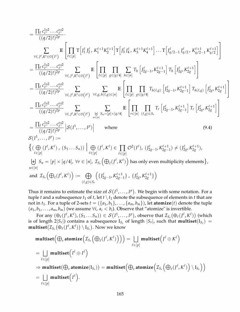
=∏` c1
` !2 . . . cs`!
2
((q/2)!)2p ·
∑∀`, J`,K`∈O(I`)
E
∏`∈[p]
T[
J`1 J`2 , K`+11 K`+1
2
]T[
J`3 J`4 , K`+13 K`+1
4
]. . . T
[J`q/2−1 J`q/2 , K`+1
q/2−1 K`+1q/2
]=
∏` c1` !2 . . . cs
`!2
((q/2)!)2p ∑∀`, J`,K`∈O(I`)
E
∏`∈[p]
∏g∈[q/4]
∑h∈[n]
Th
[J`2g−1, K`+1
2g−1
]Th
[J`2g, K`+1
2g
]=
∏` c1` !2 . . . cs
`!2
((q/2)!)2p ∑∀`, J`,K`∈O(I`)
∑∀`,g, h(`,g)∈[n]
E
∏`∈[p]
∏g∈[q/4]
Th(`,g)
[J`2g−1, K`+1
2g−1
]Th(`,g)
[J`2g, K`+1
2g
]=
∏` c1` !2 . . . cs
`!2
((q/2)!)2p ∑∀`, J`,K`∈O(I`)
∑⊎u∈[n]
Su=[p]×[q/4]E
∏r∈[n]
∏(`,g)∈Sr
Tr
[J`2g−1, K`+1
2g−1
]Tr
[J`2g, K`+1
2g
]=
∏` c1` !2 . . . cs
`!2
((q/2)!)2p
∣∣∣S(I1, . . . , Ip)∣∣∣ where (9.4)
S(I1, . . . , Ip) :=
( ⊕`∈[p]
(J`, K`) , (S1 . . . Sn)) | ⊕`∈[p]
(J`, K`) ∈ ∏`∈[p]O2(I`), (J`2g−1, K`+1
2g−1) 6= (J`2g, K`+12g ),
⊎u∈[n]
Su = [p]× [q/4], ∀r ∈ [n], ISr
(⊕`(J`, K`)
)has only even multiplicity elements,
and ISr
(⊕`(J`, K`)
):=
⊕(`,g)∈Sr
(J`2g−1, K`+1
2g−1 , J`2g, K`+12g
)Thus it remains to estimate the size of S
(I1, . . . , Ip). We begin with some notation. For a
tuple t and a subsequence t1 of t, let t \ t1 denote the subsequence of elements in t that arenot in t1. For a tuple of 2-sets t = (a1, b1, . . . , am, bm), let atomize(t) denote the tuple(a1, b1, . . . , am, bm) (we assume ∀i, ai < bi). Observe that “atomize" is invertible.
For any (⊕
`(J`, K`), (S1 . . . Sn)) ∈ S(
I1, . . . , Ip), observe that ISr
(⊕`(J`, K`)
)(which
is of length 2|Sr|) contains a subsequence ISr of length |Sr|, such that multiset(ISr) =multiset
(ISr
(⊕`(J`, K`)
)\ ISr
). Now we know
multiset(⊕
r atomize(ISr
(⊕`(J`, K`)
)))=
⊔`∈[p]
multiset(
J` ⊕ K`)
=⊔`∈[p]
multiset(
I` ⊕ I`)
⇒ multiset(⊕
r atomize(ISr))= multiset
(⊕r atomize
(ISr
(⊕`(J`, K`)
)\ ISr
))=
⊔`∈[p]
multiset(
I`)
.
165
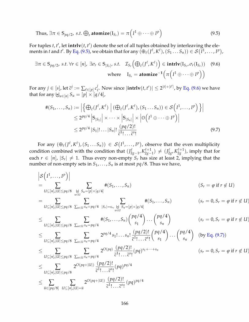
Thus, ∃π ∈ Spq/2, s.t.⊕
r atomize(ISr) = π(
I1 ⊕ · · · ⊕ Ip)
(9.5)
For tuples t, t′, let intrlv(t, t′) denote the set of all tuples obtained by interleaving the ele-ments in t and t′. By Eq. (9.5), we obtain that for any (
⊕`(J`, K`), (S1 . . . Sn)) ∈ S
(I1, . . . , Ip),
∃π ∈ Spq/2, s.t. ∀r ∈ [n], ∃σr ∈ S|Sr|, s.t. ISr
(⊕`(J`, K`)
)∈ intrlv(ISr , σr(ISr)) (9.6)
where ISr = atomize−1(
π(
I1 ⊕ · · · ⊕ Ip))
For any j ∈ [s], let cj := ∑`∈[p] cj`. Now since |intrlv(t, t′)| ≤ 2|t|+|t
′|, by Eq. (9.6) we havethat for any
⊎u∈[n] Su = [p]× [q/4],
#(S1, . . . , Sn) :=∣∣∣⊕`(J`, K`)
∣∣∣ (⊕`(J`, K`), (S1 . . . Sn)) ∈ S(
I1, . . . , Ip)∣∣∣
≤ 2pq/4∣∣∣S|S1|
∣∣∣× · · · × ∣∣∣S|Sn|
∣∣∣× ∣∣∣O(I1 ⊕ · · · ⊕ Ip)∣∣∣
≤ 2pq/4 |S1|! . . . |Sn|!(pq/2)!c1! . . . cs!
(9.7)
For any (⊕
`(J`, K`), (S1 . . . Sn)) ∈ S(
I1, . . . , Ip), observe that the even multiplicitycondition combined with the condition that (J`2g−1, K`+1
2g−1) 6= (J`2g, K`+12g ), imply that for
each r ∈ [n], |Sr| 6= 1. Thus every non-empty Sr has size at least 2, implying that thenumber of non-empty sets in S1, . . . , Sn is at most pq/8. Thus we have,∣∣∣S(I1, . . . , Ip
)∣∣∣= ∑
U⊆[n],|U|≤pq/8∑⊎
u∈USu=[p]×[q/4]
#(S1, . . . , Sn) (Sr = ϕ if r 6∈ U)
= ∑U⊆[n],|U|≤pq/8
∑∑u∈U su=pq/4
∑|Sr|=sr,
⊎u∈U
Su=[p]×[q/4]#(S1, . . . , Sn) (sr = 0, Sr = ϕ if r 6∈ U)
≤ ∑U⊆[n],|U|≤pq/8
∑∑u∈U su=pq/4
#(S1, . . . , Sn)
(pq/4
s1
). . .(
pq/4sn
)(sr = 0, Sr = ϕ if r 6∈ U)
≤ ∑U⊆[n],|U|≤pq/8
∑∑u∈U su=pq/4
2pq/4 s1! . . . sn!(pq/2)!c1! . . . cs!
(pq/4
s1
). . .(
pq/4sn
)(by Eq. (9.7))
≤ ∑U⊆[n],|U|≤pq/8
∑∑u∈U su=pq/4
2O(pq) (pq/2)!c1! . . . cs!
(pq)s1+···+sn (sr = 0, Sr = ϕ if r 6∈ U)
≤ ∑U⊆[n],|U|≤pq/8
2O(pq+|U|) (pq/2)!c1! . . . cs!
(pq)pq/4
≤ ∑u∈[pq/8]
∑U⊆[n],|U|=u
2O(pq+|U|) (pq/2)!c1! . . . cs!
(pq)pq/4
166
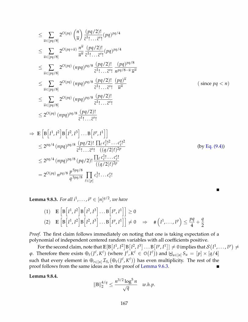
≤ ∑u∈[pq/8]
2O(pq)(
nu
)(pq/2)!c1! . . . cs!
(pq)pq/4
≤ ∑u∈[pq/8]
2O(pq+u) nu
uu(pq/2)!c1! . . . cs!
(pq)pq/4
≤ ∑u∈[pq/8]
2O(pq) (npq)pq/8 (pq/2)!c1! . . . cs!
(pq)pq/8
npq/8−u uu
≤ ∑u∈[pq/8]
2O(pq) (npq)pq/8 (pq/2)!c1! . . . cs!
(pq)u
uu ( since pq < n)
≤ ∑u∈[pq/8]
2O(pq) (npq)pq/8 (pq/2)!c1! . . . cs!
≤ 2O(pq) (npq)pq/8 (pq/2)!c1! . . . cs!
⇒ E[B[
I1, I2]B[
I2, I3]
. . . B[
Ip, I1]]
≤ 2pq/4 (npq)pq/8 (pq/2)!c1! . . . cs!
∏` c1` !2 . . . cs
`!2
((q/2)!)2p (by Eq. (9.4))
≤ 2pq/4 (npq)pq/8 (pq/2)!∏` c1
` ! . . . cs`!
((q/2)!)2p
= 2O(pq) npq/8 p 5pq/8
q 3pq/8 ∏`∈[p]
c1` ! . . . cs
`!
Lemma 9.8.3. For all i1, . . . , ip ∈ [n]q/2, we have
(1) E[B[
I1, I2]B[
I2, I3]
. . . B[
Ip, I1]]≥ 0
(2) E[B[
I1, I2]B[
I2, I3]
. . . B[
Ip, I1]]6= 0 ⇒ #
(I1, . . . , Ip
)≤ pq
4+
q2
Proof. The first claim follows immediately on noting that one is taking expectation of apolynomial of independent centered random variables with all coefficients positive.
For the second claim, note that E[B[I1, I2]B[I2, I3] . . . B
[Ip, I1]] 6= 0 implies that S
(I1, . . . , Ip) 6=
ϕ. Therefore there exists⊕
`(J`, K`) (where J`, K` ∈ O(
I`)) and
⊎u∈[n] Su = [p] × [q/4]
such that every element in⊕
r∈[n] ISr
(⊕`(J`, K`)
)has even multiplicity. The rest of the
proof follows from the same ideas as in the proof of Lemma 9.6.3.
Lemma 9.8.4.
‖B‖4/q2 ≤ n3/2 log5 n
√q
w.h.p.
167
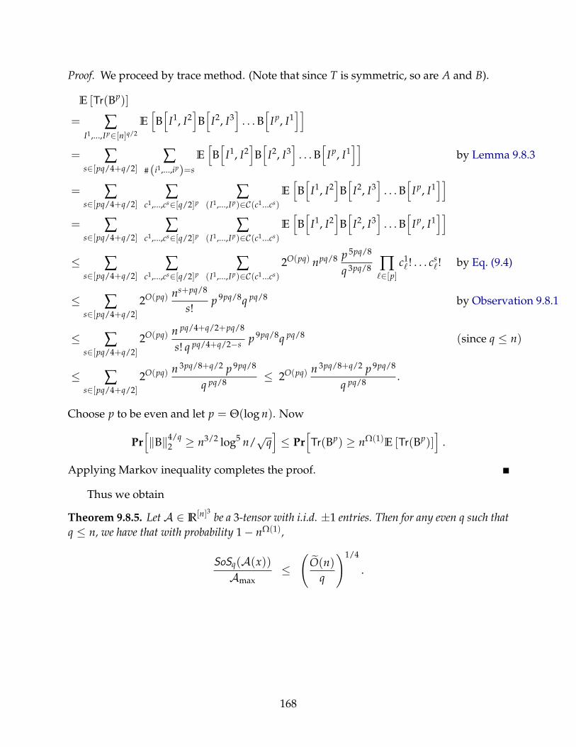
Proof. We proceed by trace method. (Note that since T is symmetric, so are A and B).
E [Tr(Bp)]
= ∑I1,...,Ip∈[n]q/2
E[B[
I1, I2]B[
I2, I3]
. . . B[
Ip, I1]]
= ∑s∈[pq/4+q/2]
∑# (i1,...,ip)=s
E[B[
I1, I2]B[
I2, I3]
. . . B[
Ip, I1]]
by Lemma 9.8.3
= ∑s∈[pq/4+q/2]
∑c1,...,cs∈[q/2]p
∑(I1,...,Ip)∈C(c1...cs)
E[B[
I1, I2]B[
I2, I3]
. . . B[
Ip, I1]]
= ∑s∈[pq/4+q/2]
∑c1,...,cs∈[q/2]p
∑(I1,...,Ip)∈C(c1...cs)
E[B[
I1, I2]B[
I2, I3]
. . . B[
Ip, I1]]
≤ ∑s∈[pq/4+q/2]
∑c1,...,cs∈[q/2]p
∑(I1,...,Ip)∈C(c1...cs)
2O(pq) npq/8 p 5pq/8
q 3pq/8 ∏`∈[p]
c1` ! . . . cs
`! by Eq. (9.4)
≤ ∑s∈[pq/4+q/2]
2O(pq) ns+pq/8
s!p 9pq/8q pq/8 by Observation 9.8.1
≤ ∑s∈[pq/4+q/2]
2O(pq) n pq/4+q/2+pq/8
s! q pq/4+q/2−s p 9pq/8q pq/8 (since q ≤ n)
≤ ∑s∈[pq/4+q/2]
2O(pq) n 3pq/8+q/2 p 9pq/8
q pq/8 ≤ 2O(pq) n 3pq/8+q/2 p 9pq/8
q pq/8 .
Choose p to be even and let p = Θ(log n). Now
Pr[‖B‖4/q
2 ≥ n3/2 log5 n/√
q]≤ Pr
[Tr(Bp) ≥ nΩ(1)E [Tr(Bp)]
].
Applying Markov inequality completes the proof.
Thus we obtain
Theorem 9.8.5. LetA ∈ IR[n]3 be a 3-tensor with i.i.d. ±1 entries. Then for any even q such thatq ≤ n, we have that with probability 1− nΩ(1),
SoSq(A(x))Amax
≤(
O(n)q
)1/4
.
168
Chapter 10
Future Directions and Perspectives onthe Approximability Landscape
10.1 Operator Norms
In this section we discuss operator norms between general normed spaces and strivetowards a characterization of their approximability. It will be convenient to have thisdiscussion in the bilinear maximization language i.e., the language of injective tensornorms with two convex sets (Fact 3.4.1 shows how operator norms can be captured bybilinear form maximization). Recall that in Chapter 1 we used ‖ · ‖C1,C2 to denote injectivetensor norm. We will abuse this notation and use ‖ · ‖X,Y to denote ‖ · ‖Ball(X),Ball(Y).
We first formalize our goal. Let (Xn)n∈N and (Ym)m∈N be sequences of norms overRn and Rm respectively. For a pair of sequences (Xn, Ym) we shall say ‖ · ‖Xn,Ym is com-putationally approximable if there exists a family of poly-sized circuits approximatingsup‖x‖Xn ,‖y‖Ym≤1〈y , Ax〉 within a constant independent of m and n (given an oracle forcomputing the norms). We are interested in the following questions:
Question. For which pairs (Xn, Ym) is the injective tensor norm computationally approximable?Can one connect the approximation factor to the geometry of Xn, Ym?
10.1.1 Approximability, Type and Cotype
Towards this characterization, evidence in the literature points to the powerful classi-fication tools of Type and Cotype from functional analysis (see Section 3.5 for a quickintroduction to these notions). Below we list various pieces of evidence that inform ourconjectures for the approximability landscape:
- In the ‖ · ‖`np,`m
q case there are constant factor approximation algorithms wheneverp, q ≥ 2 (and whenever p = 1 or q = 1) and there is complexity theoretic evidencethat no constant factor approximation algorithm exists in the other regimes. Notethat when p, q ≥ 2, C2(`
np∗), C2(`
mq∗) are bounded by absolute constants.
169
- Nesterov [Nes98] and Naor and Schechtman1 independently observed that a natu-ral computable convex programming relaxation has an integrality gap bounded byKG when X, Y are 1-unconditional norms with 2-convexity constant M(2)(·) = 1 (arich class of norms). For a 1-unconditional norm X, the Cotype-2 constant C2(X∗) iswithin a universal constant of M(2)(X) (see [LT13]). Thus if one extended the aboveresult to the case when M(2)(Xn), M(2)(Ym) are constants independent of n, m, thenone would automatically obtain such a result for the case when Cotype-2 constantsof X∗n, Y∗m are independent of n, m.
- Naor, Regev and Vidick [NRV13] algorithmicized Haagerup’s [Haa85] proof of thenon-commutative Grothendieck inequality to give a computable convex program-ming relaxation with constant integrality gap for the case of X and Y being theSchatten-∞ norm. This is an important new example as the Schatten-∞ norm is not1-unconditional (more generally it isn’t a Banach lattice) but is also the dual of theSchatten-1 norm that has Cotype-2 bounded by an absolute constant independentof the dimension.
- In Section 3.8, Section 5.3 and Section 5.8 we see that factorization through Hilbertspace is closely connected to approximation algorithms based on convex program-ming. Thus it is interesting to note that Pisier’s remarkably general factorizationtheorem (see Section 5.8) applies whenever X∗, Y∗ are Cotype-2.
Given the above, some natural questions are:
Question 1. If C2(X∗n), C2(Y∗m) = O(1) (i.e., independent of m, n), then is ‖ · ‖Xn,Ym computa-tionally approximable?
Question 2. Let Xn, Ym be such that Tp(Xn), Tp(Ym) = O(1) for some p > 1 and either C2(X∗n)grows polynomially in n or C2(Y∗m) grows polynomially in m. Then can one rule out any constantfactor approximation to ‖ · ‖Xn,Ym (ideally assuming no poly-sized family of circuits captures NP)?
Towards Question 2. As discussed in Section 2.1, combining quantitative finite dimen-sional versions of the MP+K theorem (see Theorem 13.12 in [MS09] and [AM85] for exam-ples of such theorems) with hardness results of p→ q operator norms yields quite generalhardness results in the spirit of Question 2. Recall from Section 2.1.1, that the only regimeof p → q norms for which we don’t yet have satisfactorily strong hardness results is thecase of 1 < p ≤ 2 ≤ q < ∞ (and moreover it suffices to get hardness results for the 2→ qcase where q > 2). In all other regimes there is either a polynomial time constant factorapproximation algorithm or there is complexity theoretic evidence that constant factorapproximation requires time at least 2nδ
.Strong inapproximability (SoS gaps or NP-hardness) results for the hypercontractive
2 → q case remain elusive and are closely related to obtaining hardness for polynomialmaximization over the sphere as well as the quantum separability problem (relates to longstanding open problems in quantum information theory). Consider the class of 2 → X
1personal communication
170
operator norms for exactly 2-convex norms X. This class of course contains all hyper-contractive 2 → q norms and moreover every operator norm in this class faces the samegadget reduction barrier discussed in Section 2.1.1. In Chapter 6 we show that this bar-rier can be overcome for certain exactly 2-convex norms (specifically mixed `p norms, i.e.,`q(`q′) for q, q′ > 2) and give a reduction from random label cover (for which polynomiallevel SoS gaps are available).
10.2 Degree ≥ 3
Our understanding of higher degree injective tensor norms is modest even in the specialcase of optimization over `p. In fact there are many fundamental problems surroundingoptimization over `2.
10.2.1 Hardness over the Sphere and Dense CSPs
The problem of polynomial optimization has been studied over various compact sets[Las09, DK08], and it is natural to ask how well polynomial time algorithms can approx-imate the optimum value over a given compact set (see [DK08] for a survey). While themaximum of a degree-d polynomial over the simplex admits a PTAS for every fixed d[dKLP06], the problem of optimizing even a degree 3 polynomial over the hypercube doesnot admit any approximation better than exp((log n)1−ε) (for arbitrary ε > 0) assumingNP cannot be solved in time exp((log n)O(1)) [HV04]. The approximability of polynomialoptimization on the sphere is poorly understood in comparison. Vertex based gadget re-ductions from CSPs face the same sparse optimal solution issue discussed in Section 2.1.1(see also Chapter 4 for more details). However, considering the family of constraint basedgadget reductions (i.e. replacing every arity-k constraint by a degree-k homogeneous gad-get polynomial) exposes connections to an independently interesting question. For anydegree-k polynomial a necessary condition for having all optimizers (over the sphere) be-ing well-spread is to have nk/2 non-zero coefficients. This (and some further inspectionof constraint based gadget reductions) prompts the following question:
Question 3. Can one establish APX-hardness of dense arity-k CSPs ( nk/2 constraints) overalphabet size q with a sparse predicate ( qk/2 satisfying assignments)?
10.2.2 Other Open Problems
There are still many intriguing questions to explore and the landscape is far from beingcompletely understood:
- SoS gaps/APX-Hardness for Best Separable State and APX-Hardness of maximizingpolynomials over the sphere.
- Are there subexponential (2nδ) algorithms (via SoS) for operator norm problems (like
2→4 norm, Grothendieck, Max-Cut) like those already known for unique games?
171
- Close the gap in the approximation achieved by q-levels of SoS for maximization overthe sphere. The upper bound from Chapter 8 is (n/q)d/2−1 and the best lower bound isroughly (n/qO(1))d/4−1/2 due to Hopkins et al. [HKP+17]. This is closely related to theproblem of obtaining d-XOR hard instances with maximum gap in the advantage term.
- The PTAS over the simplex due to DeKlerk, Laurent and Parillo [dKLP06] requires dd/ε2
levels of SoS. It is interesting to check if this can be improved to poly(d)/ε2. Resolvingthis question negatively would also be interesting as there are reasons to believe it willlead to improved inapproximability results for optimization over the sphere.
172
Bibliography
[AAM+11] Noga Alon, Sanjeev Arora, Rajsekar Manokaran, Dana Moshkovitz, andOmri Weinstein. Inapproximability of densest κ-subgraph from average casehardness. Manuscript, available at http://www.cs.tau.ac.il/ nogaa/PDFS/dks8.pdf,2011. 82
[ABH+05] Sanjeev Arora, Eli Berger, Elad Hazan, Guy Kindler, and Muli Safra. On non-approximability for quadratic programs. In Foundations of Computer Science,2005. FOCS 2005. 46th Annual IEEE Symposium on, pages 206–215. IEEE, 2005.12
[ABI86] Noga Alon, László Babai, and Alon Itai. A fast and simple randomized paral-lel algorithm for the maximal independent set problem. Journal of algorithms,7(4):567–583, 1986. 39
[AC+17] Antonio Auffinger, Wei-Kuo Chen, et al. Parisi formula for the ground stateenergy in the mixed p-spin model. The Annals of Probability, 45(6B):4617–4631,2017. 3
[AK06] Fernando Albiac and Nigel J Kalton. Topics in Banach space theory, volume 233of Graduate Texts in Mathematics. Springer, New York, 2006. 43, 50
[Ale03] Michael Alekhnovich. More on average case vs approximation complexity.In 44th Annual IEEE Symposium on Foundations of Computer Science, 2003. Pro-ceedings., pages 298–307. IEEE, 2003. 82
[AM85] D Amir and VD Milman. A quantitative finite-dimensional krivine theorem.Israel Journal of Mathematics, 50(1-2):1–12, 1985. 170
[AMMN06] Noga Alon, Konstantin Makarychev, Yury Makarychev, and Assaf Naor.Quadratic forms on graphs. Inventiones mathematicae, 163(3):499–522, 2006.Conference version in STOC ’05. 12
[AN04] Noga Alon and Assaf Naor. Approximating the cut-norm via Grothendieck’sinequality. In Proceedings of the 36th annual ACM symposium on Theory of com-puting, pages 72–80. ACM, 2004. 49, 54
[BBH+12] Boaz Barak, Fernando GSL Brandao, Aram W Harrow, Jonathan Kelner,David Steurer, and Yuan Zhou. Hypercontractivity, sum-of-squares proofs,
173
and their applications. In Proceedings of the forty-fourth annual ACM sympo-sium on Theory of computing, pages 307–326. ACM, 2012. 3, 9, 10, 15, 16
[BCG+12] Aditya Bhaskara, Moses Charikar, Venkatesan Guruswami, Aravindan Vi-jayaraghavan, and Yuan Zhou. Polynomial integrality gaps for strong sdprelaxations of densest k-subgraph. In Proceedings of the twenty-third annualACM-SIAM symposium on Discrete Algorithms, pages 388–405. SIAM, 2012. 83
[BdOFV14] Jop Briët, Fernando Mário de Oliveira Filho, and Frank Vallentin.Grothendieck inequalities for semidefinite programs with rank constraint.Theory Of Computing, 10(4):77–105, 2014. 64
[BGG+17] Vijay Bhattiprolu, Mrinalkanti Ghosh, Venkatesan Guruswami, EuiwoongLee, and Madhur Tulsiani. Weak decoupling, polynomial folds and approxi-mate optimization over the sphere. In Foundations of Computer Science (FOCS),2017 IEEE 58th Annual Symposium on, pages 1008–1019. IEEE, 2017. 7
[BGG+18a] V. Bhattiprolu, M. Ghosh, V. Guruswami, E. Lee, and M. Tulsiani. Inapprox-imability of Matrix p→ q Norms. ArXiv e-prints, February 2018. 7
[BGG+18b] Vijay Bhattiprolu, Mrinalkanti Ghosh, Venkatesan Guruswami, EuiwoongLee, and Madhur Tulsiani. Approximating operator norms via generalizedkrivine rounding. CoRR, abs/1804.03644, 2018. 7
[BGK+01] Andreas Brieden, Peter Gritzmann, Ravindran Kannan, Victor Klee, LászlóLovász, and Miklós Simonovits. Deterministic and randomized polynomial-time approximation of radii. Mathematika, 48(1-2):63–105, 2001. 94, 142, 143
[BGL16] Vijay Bhattiprolu, Venkatesan Guruswami, and Euiwoong Lee. Certifyingrandom polynomials over the unit sphere via sum of squares hierarchy. arXivpreprint arXiv:1605.00903, 2016. 7, 95, 146
[BH13] Fernando GSL Brandao and Aram W Harrow. Quantum de finetti theoremsunder local measurements with applications. In Proceedings of the forty-fifthannual ACM symposium on Theory of computing, pages 861–870. ACM, 2013. 16
[BH15] Fernando GSL Brandao and Aram W Harrow. Estimating operator normsusing covering nets. arXiv preprint arXiv:1509.05065, 2015. 9, 95
[BHK+16] Boaz Barak, Samuel B Hopkins, Jonathan Kelner, Pravesh K Kothari, AnkurMoitra, and Aaron Potechin. A nearly tight sum-of-squares lower bound forthe planted clique problem. In Proceedings of the 57th annual IEEE symposiumon Foundations of Computer Science, FOCS ’16, pages 428–437, 2016. 94, 105,137
[Bis11] Punyashloka Biswal. Hypercontractivity and its applications. arXiv preprintarXiv:1101.2913, 2011. 9
174
[BKS12] Boaz Barak, Guy Kindler, and David Steurer. On the optimality of re-laxations for average-case and generalized constraint satisfaction problems.Manuscript, available from http://www.boazbarak.org/research.html, 2012. 82
[BKS14] Boaz Barak, Jonathan A Kelner, and David Steurer. Rounding sum-of-squares relaxations. In Proceedings of the 46th Annual ACM Symposium onTheory of Computing, pages 31–40. ACM, 2014. 15, 16, 86, 88, 94, 95
[BKS15] Boaz Barak, Jonathan A Kelner, and David Steurer. Dictionary learning andtensor decomposition via the sum-of-squares method. In Proceedings of theForty-Seventh Annual ACM on Symposium on Theory of Computing, pages 143–151. ACM, 2015. 4, 15
[BKS17] Boaz Barak, Pravesh Kothari, and David Steurer. Quantum entanglement,sum of squares, and the log rank conjecture. arXiv preprint arXiv:1701.06321,2017. 16
[BM15] Gérard Biau and David M Mason. High-dimensional p-norms. In Mathemat-ical Statistics and Limit Theorems, pages 21–40. Springer, 2015. 37
[BMMN13] Mark Braverman, Konstantin Makarychev, Yury Makarychev, and AssafNaor. The Grothendieck constant is strictly smaller than Krivine’s bound.In Forum of Mathematics, Pi, volume 1. Cambridge University Press, 2013.Conference version in FOCS ’11. 13
[BRS15] Jop Briët, Oded Regev, and Rishi Saket. Tight hardness of the non-commutative Grothendieck problem. In Foundations of Computer Science(FOCS), 2015 IEEE 56th Annual Symposium on, pages 1108–1122. IEEE, 2015.12, 15, 28, 33, 34, 35
[BS14] Boaz Barak and David Steurer. Sum-of-squares proofs and the quest towardoptimal algorithms. arXiv preprint arXiv:1404.5236, 2014. 87
[BT87] Jean Bourgain and Lior Tzafriri. Invertibility of large submatrices with ap-plications to the geometry of banach spaces and harmonic analysis. Israeljournal of mathematics, 57(2):137–224, 1987. 50
[BV09] S Charles Brubaker and Santosh S Vempala. Random tensors and plantedcliques. In Approximation, Randomization, and Combinatorial Optimization. Al-gorithms and Techniques, pages 406–419. Springer, 2009. 15
[BV11] Aditya Bhaskara and Aravindan Vijayaraghavan. Approximating matrix p-norms. In Proceedings of the twenty-second annual ACM-SIAM symposium onDiscrete Algorithms, pages 497–511. SIAM, 2011. 11, 27, 29, 40, 41
[Cha12] Sourav Chatterjee. The missing log in large deviations for triangle counts.Random Structures & Algorithms, 40(4):437–451, 2012. 104
175
[DFJP74] Wayne J Davis, Tadeusz Figiel, William B Johnson, and AleksanderPełczynski. Factoring weakly compact operators. Journal of Functional Analy-sis, 17(3):311–327, 1974. 25
[DK08] Etienne De Klerk. The complexity of optimizing over a simplex, hypercubeor sphere: a short survey. Central European Journal of Operations Research,16(2):111–125, 2008. 4, 93, 171
[DK12a] Bobby DeMarco and Jeff Kahn. Upper tails for triangles. Random Structures& Algorithms, 40(4):452–459, 2012. 104
[DK12b] Robert DeMarco and Jeff Kahn. Tight upper tail bounds for cliques. RandomStructures & Algorithms, 41(4):469–487, 2012. 104
[dKL19] Etienne de Klerk and Monique Laurent. Convergence analysis of a lasserrehierarchy of upper bounds for polynomial minimization on the sphere. arXivpreprint arXiv:1904.08828, 2019. 15, 16, 94
[dKLP06] Etienne de Klerk, Monique Laurent, and Pablo A Parrilo. A PTAS for theminimization of polynomials of fixed degree over the simplex. TheoreticalComputer Science, 361(2):210–225, 2006. 99, 171, 172
[dKLS14] Etienne de Klerk, Monique Laurent, and Zhao Sun. Convergence analysisfor Lasserre’s measure–based hierarchy of upper bounds for polynomial op-timization. arXiv preprint arXiv:1411.6867, 2014. 15, 92
[dKLS15] Etienne de Klerk, Monique Laurent, and Zhao Sun. An alternative proof of aPTAS for fixed-degree polynomial optimization over the simplex. Mathemat-ical Programming, 151(2):433–457, 2015. 99
[DlPG12] Victor De la Pena and Evarist Giné. Decoupling: from dependence to indepen-dence. Springer Science & Business Media, 2012. 92
[DM15] Yash Deshpande and Andrea Montanari. Improved sum-of-squares lowerbounds for hidden clique and hidden submatrix problems. In COLT, pages523–562, 2015. 137
[DW12] Andrew C Doherty and Stephanie Wehner. Convergence of sdp hier-archies for polynomial optimization on the hypersphere. arXiv preprintarXiv:1210.5048, 2012. 6, 15, 16, 92, 94
[Fay04] Leonid Faybusovich. Global optimization of homogeneous polynomials onthe simplex and on the sphere. In Frontiers in global optimization, pages 109–121. Springer, 2004. 15, 94
[Fei02] Uriel Feige. Relations between average case complexity and approximationcomplexity. In Proceedings of the thiry-fourth annual ACM symposium on Theoryof computing, pages 534–543. ACM, 2002. 82
176
[FLM77] Tadeusz Figiel, Joram Lindenstrauss, and Vitali D Milman. The dimension ofalmost spherical sections of convex bodies. Acta Mathematica, 139(1):53–94,1977. 22
[FV+62] David G Feingold, Richard S Varga, et al. Block diagonally dominant ma-trices and generalizations of the gerschgorin circle theorem. Pacific J. Math,12(4):1241–1250, 1962. 117
[GLS12] Martin Grötschel, László Lovász, and Alexander Schrijver. Geometric algo-rithms and combinatorial optimization, volume 2. Springer Science & BusinessMedia, 2012. 5
[GM15] Rong Ge and Tengyu Ma. Decomposing overcomplete 3rd order tensors us-ing sum-of-squares algorithms. Approximation, Randomization, and Combina-torial Optimization. Algorithms and Techniques, page 829, 2015. 4, 15
[Gro53] Alexander Grothendieck. Résumé de la théorie métrique des produits ten-soriels topologiques. Bol. Soc. Mat. São Paulo 8, 1953. 12, 25, 50
[Gro14] Leonard Gross. Hypercontractivity, logarithmic sobolev inequalities, and ap-plications: a survey of surveys. Diffusion, quantum theory, and radically elemen-tary mathematics, pages 45–74, 2014. 3
[GRSW16] Venkatesan Guruswami, Prasad Raghavendra, Rishi Saket, and Yi Wu. By-passing UGC from some optimal geometric inapproximability results. ACMTransactions on Algorithms (TALG), 12(1):6, 2016. Conference version in SODA’12. 5, 12, 28, 31, 33, 45
[GW95] Michel X Goemans and David P Williamson. Improved approximation algo-rithms for maximum cut and satisfiability problems using semidefinite pro-gramming. Journal of the ACM (JACM), 42(6):1115–1145, 1995. 3
[Haa81] Uffe Haagerup. The best constants in the khintchine inequality. Studia Math-ematica, 70(3):231–283, 1981. 39, 49, 64, 68
[Haa85] Uffe Haagerup. The grothendieck inequality for bilinear forms on C*-algebras. Advances in Mathematics, 56(2):93–116, 1985. 3, 170
[HKP+17] Samuel B Hopkins, Pravesh K Kothari, Aaron Potechin, Prasad Raghaven-dra, Tselil Schramm, and David Steurer. The power of sum-of-squares fordetecting hidden structures. In 2017 IEEE 58th Annual Symposium on Founda-tions of Computer Science (FOCS), pages 720–731. IEEE, 2017. 17, 93, 105, 147,172
[HLZ10] Simai He, Zhening Li, and Shuzhong Zhang. Approximation algorithms forhomogeneous polynomial optimization with quadratic constraints. Mathe-matical Programming, 125(2):353–383, 2010. 15, 16, 94, 98, 108, 144
177
[HM13] Aram W Harrow and Ashley Montanaro. Testing product states, quantumMerlin-Arthur games and tensor optimization. Journal of the ACM (JACM),60(1):3, 2013. 9, 29, 40
[HNW16] Aram W Harrow, Anand Natarajan, and Xiaodi Wu. Limitations of semidef-inite programs for separable states and entangled games. arXiv preprintarXiv:1612.09306, 2016. 9, 16
[HSS15] Samuel B Hopkins, Jonathan Shi, and David Steurer. Tensor principal compo-nent analysis via sum-of-square proofs. In Proceedings of The 28th Conferenceon Learning Theory, pages 956–1006, 2015. 4, 15, 146, 163
[HV04] Johan Håstad and Srinivasan Venkatesh. On the advantage over a randomassignment. Random Structures & Algorithms, 25(2):117–149, 2004. 171
[Ind06] Piotr Indyk. Stable distributions, pseudorandom generators, embeddings,and data stream computation. Journal of the ACM (JACM), 53(3):307–323,2006. 43
[JOR04] Svante Janson, Krzysztof Oleszkiewicz, and Andrzej Rucinski. Uppertails for subgraph counts in random graphs. Israel Journal of Mathematics,142(1):61–92, 2004. 104
[Kho02] Subhash Khot. Hardness results for coloring 3-colorable 3-uniform hyper-graphs. In Foundations of Computer Science, 2002. Proceedings. The 43rd AnnualIEEE Symposium on, pages 23–32. IEEE, 2002. 31
[KMOW17] Pravesh K Kothari, Ryuhei Mori, Ryan O’Donnell, and David Witmer. Sumof squares lower bounds for refuting any csp. arXiv preprint arXiv:1701.04521,2017. 105, 146
[KMTV11] Amit Kumar, Rajsekar Manokaran, Madhur Tulsiani, and Nisheeth K Vish-noi. On lp-based approximability for strict csps. In Proceedings of the twenty-second annual ACM-SIAM symposium on Discrete Algorithms, pages 1560–1573.SIAM, 2011. 5
[KN08] Subhash Khot and Assaf Naor. Linear equations modulo 2 and the l_1 diam-eter of convex bodies. SIAM Journal on Computing, 38(4):1448–1463, 2008. 16,94, 98, 142, 143
[KN09] Subhash Khot and Assaf Naor. Approximate kernel clustering. Mathematika,55(1-2):129–165, 2009. 12
[KN11] Subhash Khot and Assaf Naor. Grothendieck-type inequalities in combina-torial optimization. arXiv preprint arXiv:1108.2464, 2011. 2
[KN12] Subhash Khot and Assaf Naor. Grothendieck-type inequalities in combinato-rial optimization. Communications on Pure and Applied Mathematics, 65(7):992–1035, 2012. 8
178
[KNS10] Guy Kindler, Assaf Naor, and Gideon Schechtman. The UGC hardnessthreshold of the Lp Grothendieck problem. Mathematics of Operations Re-search, 35(2):267–283, 2010. Conference version in SODA ’08. 12, 45, 46
[KO09] Subhash Khot and Ryan O’Donnell. SDP gaps and UGC-hardness for Max-Cut-Gain. Theory OF Computing, 5:83–117, 2009. 12
[Kri77] Jean-Louis Krivine. Sur la constante de Grothendieck. CR Acad. Sci. Paris Ser.AB, 284(8):A445–A446, 1977. 12, 13, 49
[KV04] Jeong Han Kim and Van H Vu. Divide and conquer martingales and thenumber of triangles in a random graph. Random Structures & Algorithms,24(2):166–174, 2004. 104
[Kwa72a] Stanislaw Kwapien. Isomorphic characterizations of inner product spacesby orthogonal series with vector valued coefficients. Stud. Math., 44:583–595,1972. 22, 25, 50
[Kwa72b] Stanislaw Kwapien. On operators factorizable through lp space. Mémoires dela Société Mathématique de France, 31:215–225, 1972. 25
[Las09] Jean Bernard Lasserre. Moments, positive polynomials and their applications,volume 1. World Scientific, 2009. 15, 94, 171
[Lau09] Monique Laurent. Sums of squares, moment matrices and optimization overpolynomials. In Emerging applications of algebraic geometry, pages 157–270.Springer, 2009. 15, 87, 92, 94
[Loz03] Daniel W. Lozier. NIST digital library of mathematical functions. Annals ofMathematics and Artificial Intelligence, 38(1):105–119, May 2003. 60, 61, 69
[LP68] Joram Lindenstrauss and Aleksander Pełczynski. Absolutely summing oper-ators in Lp-spaces and their applications. Studia Mathematica, 29(3):275–326,1968. 25
[LS91] László Lovász and Alexander Schrijver. Cones of matrices and set-functionsand 0–1 optimization. SIAM journal on optimization, 1(2):166–190, 1991. 5
[LS+09] Troy Lee, Adi Shraibman, et al. Lower bounds in communication complexity.Foundations and Trends R© in Theoretical Computer Science, 3(4):263–399, 2009. 2
[LT13] Joram Lindenstrauss and Lior Tzafriri. Classical Banach spaces II: functionspaces, volume 97. Springer Science & Business Media, 2013. 170
[LZ16] Eyal Lubetzky and Yufei Zhao. On the variational problem for upper tails insparse random graphs. Random Structures & Algorithms, 2016. 104
[Mau74] Bernard Maurey. Théorèmes de factorisation pour les opérateurs à valeursdans un espace lp. Séminaire Analyse fonctionnelle (dit), pages 1–5, 1974. 25, 50
179
[MR14] Andrea Montanari and Emile Richard. A statistical model for tensor PCA. InAdvances in Neural Information Processing Systems, pages 2897–2905, 2014. 4,15, 146
[MS09] Vitali D Milman and Gideon Schechtman. Asymptotic theory of finite dimen-sional normed spaces: Isoperimetric inequalities in riemannian manifolds, volume1200. Springer, 2009. 170
[Nes98] Yurii Nesterov. Semidefinite relaxation and nonconvex quadratic optimiza-tion. Optimization methods and software, 9(1-3):141–160, 1998. 12, 13, 24, 76,170
[NR14] Assaf Naor and Oded Regev. Krivine schemes are optimal. Proceedings of theAmerican Mathematical Society, 142(12):4315–4320, 2014. 13, 49, 64
[NRV13] Assaf Naor, Oded Regev, and Thomas Vidick. Efficient rounding for the non-commutative grothendieck inequality. In Proceedings of the forty-fifth annualACM symposium on Theory of computing, pages 71–80. ACM, 2013. 3, 170
[NWY00] Yuri Nesterov, Henry Wolkowicz, and Yinyu Ye. Semidefinite programmingrelaxations of nonconvex quadratic optimization. In Handbook of semidefiniteprogramming, pages 361–419. Springer, 2000. 24
[OZ13] Ryan O’Donnell and Yuan Zhou. Approximability and proof complexity. InProceedings of the Twenty-Fourth Annual ACM-SIAM Symposium on Discrete Al-gorithms, pages 1537–1556. Society for Industrial and Applied Mathematics,2013. 89
[Pie67] Albrecht Pietsch. Absolut p-summierende abbildungen in normierten räu-men. Studia Mathematica, 28(3):333–353, 1967. 25
[Pis78] Gilles Pisier. Grothendieck’s theorem for noncommutative C*-algebras, withan appendix on grothendieck’s constants. Journal of Functional Analysis,29(3):397–415, 1978. 3
[Pis80] Gilles Pisier. Un theoreme sur les operateurs lineaires entre espaces de ba-nach qui se factorisent par un espace de hilbert. In Annales scientifiques delEcole Normale Superieure, volume 13, pages 23–43. Elsevier, 1980. 25, 50
[Pis86] Gilles Pisier. Factorization of linear operators and geometry of Banach spaces.Number 60. American Mathematical Soc., 1986. 2, 25, 50
[Pis12] Gilles Pisier. Grothendieck’s theorem, past and present. Bulletin of the Ameri-can Mathematical Society, 49(2):237–323, 2012. 2, 8
[Rag08] Prasad Raghavendra. Optimal algorithms and inapproximability results forevery csp? In Proceedings of the fortieth annual ACM symposium on Theory ofcomputing, pages 245–254. ACM, 2008. 5
180
[Ree91] JA Reeds. A new lower bound on the real Grothendieck constant.Manuscript, 1991. 12
[Ros73] Haskell P Rosenthal. On subspaces of lp. Annals of Mathematics, pages 344–373, 1973. 25
[RRS16] Prasad Raghavendra, Satish Rao, and Tselil Schramm. Strongly refuting ran-dom csps below the spectral threshold. arXiv preprint arXiv:1605.00058, 2016.i, 6, 15, 17, 95, 96, 137, 146, 149
[RS09] Prasad Raghavendra and David Steurer. Towards computing theGrothendieck constant. In Proceedings of the Twentieth Annual ACM-SIAMSymposium on Discrete Algorithms, pages 525–534. Society for Industrial andApplied Mathematics, 2009. 5, 12, 13
[RS10] Prasad Raghavendra and David Steurer. Graph expansion and the uniquegames conjecture. In Proceedings of the 42nd annual ACM Symposium on Theoryof Computing, pages 755–764. ACM, 2010. 9
[RV15] Oded Regev and Thomas Vidick. Quantum xor games. ACM Transactions onComputation Theory (ToCT), 7(4):15, 2015. 3
[SA90] Hanif D Sherali and Warren P Adams. A hierarchy of relaxations betweenthe continuous and convex hull representations for zero-one programmingproblems. SIAM Journal on Discrete Mathematics, 3(3):411–430, 1990. 5
[Sch87] Gideon Schechtman. More on embedding subspaces of Lp in `nr . Compositio
Math, 61(2):159–169, 1987. 29, 41, 42
[Sch06] Gideon Schechtman. Two observations regarding embedding subsets of eu-clidean spaces in normed spaces. Advances in Mathematics, 200(1):125–135,2006. 37
[Sim98] Barry Simon. The classical moment problem as a self-adjoint finite differenceoperator. Advances in Mathematics, 137(1):82–203, 1998. 157
[So11] Anthony Man-Cho So. Deterministic approximation algorithms for sphereconstrained homogeneous polynomial optimization problems. Mathematicalprogramming, 129(2):357–382, 2011. 16, 94, 98, 142, 144
[Ste61] Sergei Borisovich Stechkin. On best lacunary systems of functions. IzvestiyaRossiiskoi Akademii Nauk. Seriya Matematicheskaya, 25(3):357–366, 1961. 39
[Ste05] Daureen Steinberg. Computation of matrix norms with applications to robustoptimization. Research thesis, Technion-Israel University of Technology, 2005. 9,11, 12, 14, 15
181
[Tro09] Joel A Tropp. Column subset selection, matrix factorization, and eigenvalueoptimization. In Proceedings of the Twentieth Annual ACM-SIAM Symposium onDiscrete Algorithms, pages 978–986. Society for Industrial and Applied Math-ematics, 2009. 50, 75
[TS14] R. Tomioka and T. Suzuki. Spectral norm of random tensors. ArXiv e-prints,July 2014. 145, 149
[vB72] Paul van Beek. An application of Fourier methods to the problem of sharp-ening the Berry-Esseen inequality. Zeitschrift für Wahrscheinlichkeitstheorie undverwandte Gebiete, 23(3):187–196, 1972. 46
[Ver17] Roman Vershynin. High Dimensional Probability. 2017. 29, 37
[Vu01] Van H Vu. A large deviation result on the number of small subgraphs of arandom graph. Combinatorics, Probability & Computing, 10(1):79–94, 2001. 104
182